| Issue |
A&A
Volume 699, July 2025
|
|
|---|---|---|
| Article Number | A141 | |
| Number of page(s) | 22 | |
| Section | Cosmology (including clusters of galaxies) | |
| DOI | https://doi.org/10.1051/0004-6361/202554743 | |
| Published online | 04 July 2025 | |
CHEX-MATE: Multiprobe analysis of Abell 1689
1
Université Paris Saclay, IRFU/CEA, 91191 Gif-sur-Yvette, France
2
Department of Astronomy, University of Geneva, Ch. d’Ecogia 16, CH-1290 Versoix, Switzerland
3
INAF, Osservatorio di Astrofisica e Scienza dello Spazio, Via Piero Gobetti 93/3, 40129 Bologna, Italy
4
California Institute of Technology, 1200 E. California Blvd., MC 367-17, Pasadena, CA 91125, USA
5
Korea Advanced Institute of Science and Technology (KAIST), 291 Daehak-ro, Yuseong-gu, Daejeon 34141, Republic of Korea
6
INAF, IASF-Milano, via A. Corti 12, 20133 Milano, Italy
7
Academia Sinica Institute of Astronomy and Astrophysics (ASIAA), No. 1, Section 4, Roosevelt Road, Taipei 10617, Taiwan
8
Laboratoire d’Astrophysique de Marseille, Aix-Marseille Univ., CNRS, CNES, Marseille, France
9
Institut d’Astrophysique de Paris, UMR7095 CNRS & Sorbonne Université, 98bis Bd Arago, F-75014 Paris, France
10
IRAP, CNRS, Université de Toulouse, CNES, UT3-UPS, Toulouse, France
11
INFN, Sezione di Bologna, viale Berti Pichat 6/2, 40127 Bologna, Italy
12
Dipartimento di Fisica, Università degli studi di Roma Tor Vergata, Via della Ricerca Scientifica 1, I-00133 Roma, Italy
13
INFN, Sezione di Roma ‘Tor Vergata’, Via della Ricerca Scientifica 1, 00133 Roma, Italy
14
INAF – Istituto di Radioastronomia, via P. Gobetti 101, I-40129 Bologna, Italy
15
Dip. Fisica, Sapienza Università di Roma, Piazzale Aldo Moro 5, 00185 Roma, Italy
16
Michigan State University, Physics & Astronomy Department, 567 Wilson Rd, East Lansing, MI 48824, USA
17
Department of Physics, Informatics and Mathematics, University of Modena and Reggio Emilia, 41125 Modena, Italy
18
Dipartimento di Fisica e Astronomia (DIFA), Alma Mater Studiorum – Università di Bologna, via Gobetti 93/2, 40129 Bologna, Italy
19
HH Wills Physics Laboratory, University of Bristol, Bristol, UK
20
INFN – Sezione di Genova, Via Dodecaneso 33, 16146 Genova, Italy
21
INAF – Osservatorio Astronomico di Trieste, via Tiepolo 11, I-34131 Trieste, Italy
22
IFPU, Institute for Fundamental Physics of the Universe, Via Beirut 2, 34014 Trieste, Italy
23
Department of Physics; University of Michigan, Ann Arbor, MI 48109, USA
24
INAF – Osservatorio astronomico di Padova, vicolo dell’Osservatorio 5, I-35122 Padova, Italy
⋆ Corresponding author: loris.chappuis@cea.fr
Received:
25
March
2025
Accepted:
2
May
2025
The nature of the elusive dark matter can be probed by comparing the predictions of the cold dark matter framework with the gravitational field of massive galaxy clusters. However, a robust test of dark matter can only be achieved if the systematic uncertainties in the reconstruction of the gravitational potential are minimized. Techniques based on the properties of intracluster gas rely on the assumption that the gas is in hydrostatic equilibrium within the potential well, whereas gravitational lensing is sensitive to projection effects. Here we attempt to minimize systematics in galaxy cluster mass reconstructions by jointly exploiting the weak gravitational lensing signal and the properties of the hot intracluster gas determined from X-ray and millimeter (Sunyaev-Zel’dovich) observations. We constructed a model to fit the multiprobe information within a common framework, accounting for non-thermal pressure support and elongation of the dark matter halo along the line of sight. We then applied our framework to the massive cluster Abell 1689, which features unparalleled multiwavelength data. In accordance with previous works, we find that the cluster is significantly elongated along the line of sight. Accounting for line-of-sight projections, we require a non-thermal pressure support of 30 − 40% at r500 to match the gas and weak lensing observables. The joint model retrieves a concentration c200 ∼ 7, which is lower and better agrees with the concentration-mass relation than the high concentration retrieved from weak lensing data alone under the assumption of spherical symmetry (c200 ∼ 15). Applying our method to a larger sample will allow us to study the shape of dark matter mass profiles and the level of non-thermal pressure support in galaxy clusters at the same time.
Key words: gravitational lensing: weak / galaxies: clusters: general / galaxies: clusters: intracluster medium / galaxies: clusters: individual: A1689 / dark matter / X-rays: galaxies: clusters
© The Authors 2025
 Open Access article, published by EDP Sciences, under the terms of the Creative Commons Attribution License (https://creativecommons.org/licenses/by/4.0), which permits unrestricted use, distribution, and reproduction in any medium, provided the original work is properly cited.
This article is published in open access under the Subscribe to Open model. Subscribe to A&A to support open access publication.
1. Introduction
Galaxy clusters are the most massive gravitationally bound structures in the Universe. According to the hierarchical structure formation scenario, they developed from primordial overdensities during the early Universe, evolving through mergers and accretion until they attained masses around 1014–1015 M⊙ in the present day (Kravtsov & Borgani 2012). While galaxy clusters can be observed out to z ∼ 2, in the bottom-up structure formation scenario the most massive clusters are found at low redshifts. Primordial gas is trapped and heated in the gravitational well of the dark matter halo, reaching temperatures on the order of 107 − 108 K. Referred to as the intracluster medium (ICM), this diffuse and hot plasma accounts for the majority (∼90%) of the baryonic content of galaxy clusters, representing 10–15% of the total mass. In contrast, the hundreds to thousands of galaxies within the cluster contribute to the stellar mass, which only constitutes 1–2% of the total mass. Most of the mass content is in the form of dark matter (DM), which accounts for the remaining 85% (Gonzalez et al. 2013; Chiu et al. 2018a; Eckert et al. 2022b).
Tracing the nodes of the cosmic web, galaxy clusters serve as powerful cosmological probes through their mass and redshift distribution (Allen et al. 2011). The primary systematic uncertainty affecting cosmological inferences with this technique is the mass scale of the detected systems. Thanks to their multicomponent structure (ICM, galaxies, and DM), galaxy clusters offer multiple observables from which one can constrain the astrophysical processes and recover improved mass measurements (Pratt et al. 2019).
In this work, we focus on three of these observables: X-ray emission, the Sunyaev-Zel’dovich (SZ) effect, and weak gravitational lensing. Being almost fully ionized, the ICM emits X-rays via thermal bremsstrahlung and line emission. Cosmic microwave background (CMB) photons crossing the ICM can get inverse-Compton scattered by high-energy electrons of the ICM, resulting in an observable spectral shift known as the SZ effect. The radial properties of the thermodynamic quantities of the ICM are set by the total gravitational potential of the system. When dark matter dominates the mass content, one can consider the X-ray emission and SZ signal to be indirect observables of the DM distribution (Bulbul et al. 2010; Capelo et al. 2012; Ettori et al. 2023). Assuming that the gas pressure balances gravity, the total mass of the cluster can be inferred. A more direct probe of the underlying mass is through gravitational lensing. The deep gravitational potential of a galaxy cluster acts as a lens and changes the path of the light emitted by background galaxies, and modifies their apparent shapes and sizes (Bartelmann & Schneider 2001; Kneib & Natarajan 2011; Hoekstra et al. 2013). This deformation is only dependent on the surface mass density, Σ, of the lens in the plane of the sky and the distances to the lens and the background sources. In this study, we utilize the weak lensing (WL) regime, which is applicable when the lensing signal is measured at a distance from the center of the lens where the surface mass density is low compared to the critical value, Σcrit (Umetsu 2020). In this regime, two main effects are observed: shear (γ), which increases the ellipticity of the source, and convergence (κ), which increases the size of the source. As implied by its name, the weak gravitational lensing signal is subtle and requires statistical measurement across multiple sources to be detected reliably.
Assuming hydrostatic equilibrium (HSE), X-ray and SZ observations of galaxy clusters that are well spatially resolved can be used to infer a hydrostatic mass profile (Pointecouteau & Silk 2005; Vikhlinin et al. 2006). While traditionally the hydrostatic mass was reconstructed using X-ray surface brightness and spectroscopic temperature, in recent years this framework has been extended to model the SZ signal (Ameglio et al. 2007; Ettori et al. 2019; Muñoz-Echeverría et al. 2023; Mastromarino et al. 2024). This can be achieved by forward modeling a chosen density profile parameterization to the X-ray and SZ data (Eckert et al. 2022a).
Reconstructions of mass profiles based on gas properties assume that the gas is in equilibrium within the potential well set by the DM and that the energy is fully thermalized. Galaxy cluster masses determined through this technique show a systematic underestimation when compared to weak lensing measurements: the hydrostatic mass bias (von der Linden et al. 2014; Hoekstra et al. 2015; Okabe & Smith 2016; Medezinski et al. 2017; Sereno et al. 2017a; Herbonnet et al. 2020). By assuming the gas pressure to be exclusively thermal, the recovered mass will be underestimated if an additional pressure component of non-thermal origin partakes in the total pressure of the ICM. Simulations show that non-thermal pressure support can indeed represent a significant contribution to the total pressure, and increases at large radii where gas tends to be less relaxed (Lau et al. 2009; Meneghetti et al. 2010; Rasia et al. 2012; Angelinelli et al. 2020; Barnes et al. 2021; Bennett & Sijacki 2022).
On the other hand, cluster masses estimated using gravitational lensing are independent of the dynamical state and are expected to be close to unbiased on average (Umetsu 2020; Grandis et al. 2021), with a remaining bias of < 20% that can be calibrated with simulations (Euclid Collaboration: Giocoli et al. 2024). Nonetheless, the weak lensing signal is strongly impacted by projection effects. Due to their formation history, galaxy clusters are expected to exhibit triaxial shapes (De Filippis et al. 2005; Lau et al. 2011; Limousin et al. 2013; Sereno et al. 2018; Lau et al. 2020), and the alignment of their major axis with the line of sight will result in a boosted weak lensing signal (Gavazzi 2005; Sereno & Umetsu 2011; Chen et al. 2020; Wu et al. 2022; Euclid Collaboration: Giocoli et al. 2024). Assuming random orientations of the selected galaxy clusters, this orientation bias will be small on average but potentially significant on mass measurements of individual clusters (Despali et al. 2014). This can be particularly significant for the population of strong lensing clusters, for example (Hennawi et al. 2007).
Given the strengths and weaknesses of the various mass reconstruction techniques, if multiple observables are available for the same system, the accuracy of the reconstruction can be improved by jointly fitting the observables rather than considering them individually (Sereno et al. 2018). The different line-of-sight dependencies of the X-ray, SZ, and WL observables allow us to constrain the three-dimensional shape of the underlying system in a triaxial geometry (Limousin et al. 2013; Morandi et al. 2012; Sereno et al. 2013; Umetsu et al. 2015; Chiu et al. 2018b). The comparison between hydrostatic and lensing measurements also provides constraints on deviations from hydrostatic equilibrium (Sayers et al. 2021; Umetsu et al. 2022). The expected improvement in WL data quality thanks to upcoming wide-field telescopes like Euclid and Rubin calls for a substantial effort in the modeling of galaxy cluster properties.
In this paper, we develop a novel model to reconstruct galaxy cluster mass profiles from multiprobe observations (X-ray, WL, SZ). This joint analysis aims to fit a parameterized density profile to the entire dataset. By adding two additional ingredients, line of sight (hereafter LOS) elongation and non-thermal pressure support, we provide a framework that is well suited for the analysis of massive clusters with high data quality. As a test case, we apply our framework to the famous lensing cluster Abell 1689, for which high-quality X-ray, WL, and SZ data exist. In Sect. 2, we present the details of our modeling for each observable. Sect. 3 introduces Abell 1689 as our case study and the details of the data extraction. Finally, Sect. 4 and Sect. 5 present our results and their interpretation, respectively.
Throughout this study, we adopt the WMAP9 cosmology (Hinshaw et al. 2013), with matter density parameter Ωm = 0.2865, cosmological constant density parameter ΩΛ = 0.7134, and Hubble constant  . All distances are given in proper units. At the redshift of A1689 (z = 0.183), this translates into 1 arcmin = 186.7 kpc. The errors displayed in our analysis results are defined as the 1σ errors, i.e., the 16th and 84th percentiles of the posterior parameter distributions.
2. Mass modeling
2.1. Mass profiles
Galaxy cluster masses are typically computed as the spherically enclosed mass within a chosen radius around the cluster center. This radius is often chosen to match a given level Δ of over-density compared to the critical density of the Universe, i.e., where  . Common choices for Δ are 200 or 500.
Using N-body simulations, Navarro et al. (1996) established the Navarro Frenk White (NFW) parameterization as a good fit to DM halo shapes in the Cold Dark Matter (CDM) paradigm across a wide range of halo masses, from dwarf galaxies to the most massive galaxy clusters (Bullock et al. 2001; Power et al. 2003; Navarro et al. 2004; Macciò et al. 2008; Klypin et al. 2016; Le Brun et al. 2017). This self-similarity of CDM halos is emphasized by the asymptotic behavior of the inner (ρ(r) = r−1) and outer (ρ(r) = r−3) slopes of the NFW profile. For a given overdensity Δ, the NFW profile reads
Here rΔ is the radius r at which  and cΔ is the concentration parameter, cΔ = rΔ/rs with rs the scale radius (defined as the radius at which the NFW slope is equal to −2). The scaled density ρs can be reformulated as a function of the critical density of the Universe ρc(z) as
Further studies found that the Einasto (1965) profile which describes the density profile as a power law with a rolling index, provides a better representation of DM profiles that stray further from the expected self-similarity in N-body simulations (Navarro et al. 2004; Klypin et al. 2016; Ludlow et al. 2016; Brown et al. 2020):
![$$ \begin{aligned} \rho _{\rm Einasto}(r) = \rho _s \exp {\left[-\frac{2}{\alpha }\left(\left( \frac{r}{r_s}\right)^{\alpha } -1 \right)\right]}, \end{aligned} $$](/articles/aa/full_html/2025/07/aa54743-25/aa54743-25-eq6.gif)
with α the shape parameter responsible of the curvature of the profile. The CDM paradigm makes strong predictions for the value α. Navarro et al. (2009) and Ludlow et al. (2016) showed that CDM halos can be well described by an Einasto profile with α ∼ 0.18, which is further supported by observations (Umetsu et al. 2014; Eckert et al. 2022b).
2.2. Observables
The different components (ICM, galaxies, DM) of galaxy clusters provide for a wide range of observables. In this work, we build a global framework to reconstruct the mass distribution within galaxy clusters by jointly fitting the gas observables – the X-ray emission and the SZ effect – and the weak gravitational lensing signal in a self-consistent way.
2.2.1. X-ray observables
Being heated to high temperatures, the ICM emits X-rays via bremsstrahlung and line emission and allows us to recover two primary observables: X-ray surface brightness and spectroscopic temperature. The observed surface brightness is the integrated emissivity of all the gas particles in a given line of sight. Each volume element will thus have a contribution Λ(T,Z)nenH with ne the electronic density, nH the proton density, and Λ(T,Z) the cooling function. In a soft X-ray energy band (e.g., 0.5–2 keV), Λ(T, Z) is roughly constant for temperatures greater than ∼2 keV. The surface brightness is then given by the gas emissivity integrated along the LOS,
The ratio of ne to nH is determined by the level of ionization of the ICM and is assumed to be constant throughout the cluster’s volume. In a fully ionized plasma ne/nH ∼ 1.17 assuming Solar abundance ratios as given in Asplund et al. (2009).
Similarly, the measured spectroscopic temperatures depend on the projection of the 3D temperatures of volume elements along the LOS:
As shown in Eq. (5), the projected temperature depends on the emissivity-dependent weight w given to each volume element, which at high temperatures (T > 3 keV) can be written as  (Mazzotta et al. 2004).
2.2.2. The Sunyaev-Zel’dovich effect
The SZ effect is the inverse Compton scattering of CMB photons with the electrons of the hot ICM. The amplitude of the resulting spectral distortion is proportional to the Compton parameter y and is directly related to the energy kBT3D of the encountered charged particles and their density ne (see Eq. (6)). As a result, the projected SZ signal is proportional to the gas pressure integrated along the LOS,
with σT the Thompson cross-section.
2.2.3. Weak gravitational lensing
The lensing signal depends on the projected mass density along the LOS, the surface mass density Σ:
where θ is the angular separation from the center of the lens.
The foreground galaxy cluster acts like a lens located between the observer and the background galaxies. Similar to the case of an optical lens, the observed signal depends on the angular diameter distances DL (distance from the observer to the lens), DS (distance from the observer to the source), and DLS (distance between the lens and the source). These quantities are encapsulated in the critical surface density
The weak lensing regime is defined as the regime where Σ ≪ Σcrit. In this regime, the lensing effect is not detectable on individual galaxies and the signal can be brought up by averaging over multiple background sources.
We briefly summarize here the main equations of cluster weak lensing. For more details we refer the reader to ?. In a polar coordinate system centered on the lens, the shear γ can be split into two geometrically defined components, the tangential shear γ+, and the 45° rotated cross shear γ× :
with γ1 and γ2 the spin-2 shear components in Cartesian coordinates and (θ, ϕ) the polar coordinates (distance to the center and azimuthal angle, respectively).
This formulation has the advantage of providing a consistent sanity check: under the approximation of weak lensing, |γ(θ)| ≪ 1, one finds
And thus, in the absence of systematics, the 45° rotated cross shear γ× must be consistent with zero. Here we have introduced the excess surface mass density ΔΣ(θ), which is defined as the difference between the average surface mass density  within a circle of radius θ and the local surface mass density,
The averaged ellipticity of the background galaxies, the reduced tangential shear g+(θ), offers a direct observable of the weak lensing effect. It is related to the shear as
with κ = Σ/Σcrit the convergence. In the linear regime:
In this work, to probe high surface mass density regions, thus considering the non-linear but subcritical regime, we will use the following formulation of the mean tangential shear (Seitz & Schneider 1997):
with

where the brackets denote the averaging over the source redshift distribution.
2.3. Modeling
This work builds upon the Python package hydromass1 (Eckert et al. 2022a), which allows to model X-ray and SZ observables jointly under the assumption that the gas is in hydrostatic equilibrium within the potential well set by the total mass distribution. Here we extend the framework to include a self-consistent modeling of WL signal and gas observables. This hybrid SZ and X-ray method uses a Bayesian forward modeling approach in which 3D quantities are sampled according to priors and then projected along the LOS to be compared with the data. The optimization is done using the No U-Turn Sampler (Hoffman & Gelman 2011) implemented within the PyMC package (Patil et al. 2010), running simultaneously 4 chains of 4000 steps each with an equal number of tuning steps.
As introduced in Eckert et al. (2020), hydromass uses a linear combination of King functions Φk(r) to model the 3D emissivity profile ϵ(r):
with αk the coefficient of the basis function Φk(r). The basis functions are chosen to be flexible enough to reproduce a wide range of profiles, under the assumption that the underlying 3D profile is smooth, positive definite and monotonically decreasing.
To infer the shape of the mass profile, two main methods are implemented within the hydromass package (Ettori et al. 2011):
-
Mass model: a functional form for the mass profile (e.g., NFW, see Eq. (1)) is assumed and the model optimizes the parameters of the mass profile to reproduce the data at hand. Assuming hydrostatic equilibrium (Eq. (17)), the 3D pressure can be recovered by integrating the modeled mass profile Mmod (Eq. (18)),
-
Parametric forward: the pressure profile is modeled as a generalized NFW (gNFW) (Nagai et al. 2007) :
The pressure profile is projected along the LOS assuming spherical symmetry and fitted to the data. The mass profile is then inferred from the best fitting 3D pressure profile.
This work focuses on the former method (mass model) by implementing an option to jointly fit the WL data with the X-ray and SZ information. To accommodate potential deviations from hydrostatic equilibrium and spherical symmetry, we introduce two additional parameters to the model: non-thermal pressure and LOS elongation. The parametric forward method is used as a reference to validate our model.
2.3.1. From density profile to mean tangential shear
Our implementation of WL in the hydromass package is fully numerical and it can thus include any parametric mass model. Here we focus on the NFW and Einasto models, which are most commonly used to describe DM halos. Following Eq. (1), the free parameters of the NFW density profile are the concentration cΔ and the overdensity radius rΔ from which the enclosed mass can easily be recovered:
We make the choice of Δ = 200 which is the most common definition of the NFW concentration (Wechsler et al. 2002; Klypin et al. 2016).
The Einasto profile (Eq. (3)) is implemented according to the optimized parameterization presented by Ettori et al. (2019). The fitted parameters are the scale radius rs, the inverse shape parameter μ = 1/α and the unitless normalization parameter cnorm such that :
![$$ \begin{aligned} \rho _s = \frac{\Delta \rho _{\rm crit}}{3}\left[\ln (1+c_{\rm norm})-\frac{c_{\rm norm}}{1+c_{\rm norm}}\right]. \end{aligned} $$](/articles/aa/full_html/2025/07/aa54743-25/aa54743-25-eq26.gif)
The priors on the model parameters for both mass models can be found in Table 1.
The first step in the numerical modeling of the mean tangential shear is to obtain the surface mass density Σ by projecting the density profile (see Eq. (7)). The surface mass density is then integrated in circular bins to compute ΔΣ according to Eq. (11). We use Eq. (14) to model the mean tangential shear, allowing us to use the non-linear but subcritical regime to probe the density profile of the cluster at lower radii than the traditional linear weak lensing approximation (Eq. (13)).
2.3.2. non-thermal pressure
Since the modeling of the gas properties assumes hydrostatic equilibrium while the WL signal does not depend on dynamical state, following Eckert et al. (2019) we modify the hydrostatic equilibrium (Eq. (17)) to include a non-thermal correction term,
with Pth and PNT the thermal and non-thermal pressure, respectively. The non-thermal pressure term therefore represents any additional pressure term that is required to balance the local gravitational field. This term is expected to be dominated by merger-induced random gas motions that have not yet thermalized (Lau et al. 2009; Nelson et al. 2014; Biffi et al. 2016; Vazza et al. 2018), although any additional non-thermal contribution from, e.g., magnetic fields or cosmic rays, is included in the non-thermal pressure term. Throughout this work, we characterize the relative importance of non-thermal pressure using the non-thermal pressure fraction,
First-order development shows that αNT ≈ 1 − MHSE/Mtot (Eckert et al. 2019; Ettori & Eckert 2022). We describe the non-thermal pressure profile using a parametric functional form and optimize for the corresponding model parameters. We test two different parameterizations of the non-thermal pressure to assess the dependence of the recovered parameters on the chosen parametric form.
-
Using a set of 20 clusters simulated at high resolution with the adaptive mesh refinement code ENZO, Angelinelli et al. (2020) showed that non-thermal pressure profiles in simulated clusters can be described as:
with r200, m the radius within which the mean density is 200 times the mean matter density of the Universe (as opposed to the critical density). This parameterization describes the radial profile of αNT as a power law (described by the parameters a0 and a1) with a central floor (a2);
-
Ettori & Eckert (2022) suggested a different parameterization of the non-thermal pressure, in which the non-thermal pressure is assumed to scale with the electron density ne similarly to the thermal pressure,
Here the index β governs the shape of the non-thermal pressure profile, n0 = 10−3 cm−3 is a scale density, and P0NT describes the non-thermal pressure at ne = n0. This functional form is motivated by the expected dependence of the various sources of non-thermal pressure (turbulence, magnetic fields, cosmic rays) on the gas density (Miniati & Beresnyak 2015). The index β is expected to be around ∼0.9 (Ettori & Eckert 2022), which is less than the polytropic index of the thermal pressure (Γ ∼ 1.2, Capelo et al. 2012; Ghirardini et al. 2019), such that generally αNT increases with radius.
To set up the priors on the parameters of the non-thermal pressure profiles, we used the set of 20 simulated clusters presented in Angelinelli et al. (2020) and fitted their non-thermal pressure profile with Eq. (25). We then used the distributions of the model parameters in the simulated sample to set up the priors on the parameters when fitting the data. The priors are broad enough to encompass the range of profiles in the simulated data set. Our implementation of the polytropic model uses a log uniform prior on P0NT and a Gaussian prior on β, and uniform priors for the Angelinelli model to remain as uninformative as possible. The priors on the parameters of both models are shown in Table 1.
2.3.3. Elongation
The model implemented here accounts for deviations from spherical symmetry by implementing a correction factor e that describes the ratio between the true projected quantity and the quantity calculated assuming spherical symmetry. While methods to reconstruct the shape parameters of DM and gas in a triaxial geometry have been developed (e.g., Sereno et al. 2017b; Kim et al. 2024), these methods are computationally expensive and still make the hypothesis of a single ellipsoidal halo. Here we attempt to account for the impact of deviations from spherical symmetry using a simpler one-dimensional correction factor.
We consider the 3D distribution X(x, y, z) of a generic quantity X (X-ray emissivity, thermal pressure, mass density) and the corresponding quantity Xp(x, y) projected along axis z (X-ray surface brightness SX, SZ Compton parameter y, or surface mass density Σ). The projected quantity is given by
The observed quantity is the circularly averaged projected profile  , with θp the projected angular radius. The discretized profile {Xp, i}i = 1N is given by the average of Xp in the circular annulus enclosed within projected angular radii θp, i and θp, i + 1, with {θp, i}i = 1N the boundaries of the defined annular bins. The measured values can therefore be written as
where x and y are the angular coordinates and Ω the corresponding solid angle.
Under spherical symmetry, this quantity can be estimated by convolving the mean discretized 3D profile {Xi}i = 1N with the projected volumes:
where the projection volumes Vs; i, j are given by the intersection of spherical shell j with cylindrical shell i (Kriss et al. 1983). In the general case where the system is not spherical, we define the elongation factor e as the mean ratio between the (a priori unknown) true 3D volumes Vt and their spherical counterparts Vs (De Filippis et al. 2005),

The meaning of the elongation factor is described in Fig. 1 for the case of a triaxial halo that is perfectly aligned with the LOS. Let {Xs, i}i = 1N be the projection of {Xi}i = 1N assuming spherical symmetry, i.e., the profile of a spherical halo with the same radial 3D profile as the actual halo (red solid circle in Fig. 1). The figure shows that the projected profile is boosted or suppressed by a factor e with respect to the spherical case, as the LOS volumes are altered. On top of that, the radial axis is stretched or compressed by a factor e1/3, such that the projected plane-of-the-sky radius is related to the spherically averaged radius as
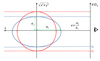 |
Fig. 1. Sketch of the implemented elongation correction. The sketch shows the isodensity surface of an ellipsoidal halo (blue solid curve) in the LOS (z) – plane of the sky ( |

Therefore, the measured radial profile is related to the spherically averaged projected profile Xs as (Sereno 2007)
As a result, every projected quantity gets modified by a factor e and stretched by a factor e1/3 with respect to the spherical case, such that the measured projected profiles become

where the quantities with the index s denote the spherically averaged profiles projected under spherical symmetry (Eq. (28)). We make the fair assumption that the observed temperature TX should not be impacted by the LOS elongation, as the elongation factors at the numerator and denominator approximately cancel out (see Eq. (5)).
At every step of our optimization process, we solve Eqs. (32) through (34) to estimate the model profile at every observed data point. Numerically solving this equation requires applying a root-finding algorithm at every point, which is computationally expensive. In a realistic case e ≈ 1, and |rs − rp|/rs ≪ 1, such that Eq. (31) can be linearly expanded:
In realistic cases, we find that the elongation-dependent correction factor in the right-hand side of Eq. (36) reproduces the true solution of Eq. (31) with an accuracy of a few percent at every radius.
In practice, the constraints on the elongation parameter e are obtained from the ratio of the pressure inferred from X-ray and SZ observations. These observations trace the exact same quantity, albeit with different LOS dependencies (see Eqs. (4), (5), (6)). Since ne ∝ SX1/2, the ratio of spherically deprojected SZ to X-ray pressure becomes (e.g., Kozmanyan et al. 2019; Ettori et al. 2020),

In a spherical halo e = 1 for every LOS. Conversely, in a generic case e is larger than 1 when the system is oriented preferentially along the LOS and smaller than 1 when the system is elongated in the plane of the sky. Therefore, the profiles corrected for elongation (Eq. (31)) correspond to the profiles one would observe along a fiducial sight line where PSZ = PX, i.e., to the spherically averaged profiles.
The Gaussian prior used on the elongation parameter can be found in Table 1. Being centered on 1 (i.e., the spherical case), it assumes that halos are randomly orientated with respect to the LOS. Lau et al. (2020) used massive halos extracted from large N-body simulations to estimate the distribution of triaxial galaxy clusters shapes. The authors found that deviations from spherical symmetry lead to variations of surface mass density of ∼20%, which we use as the width of our Gaussian prior on e. Since we model the mean tangential shear profile from the projected mass density, the way the elongation parameter e propagates (Eq. (34)) implies that we assume a common dark matter and gas geometry. The model also assumes that the impact of asphericity is constant with radius. Future versions of our code will implement a self-consistent calculation of DM and gravitational potential distributions.
3. Application to A1689: dataset
Abell 1689 is a galaxy cluster situated in the Virgo constellation at redshift z = 0.183. It is one of the most massive clusters in the observable Universe, with a mass usually found above 1015 M⊙. Thanks to its very high mass, A1689 acts as a very powerful gravitational lens. Comparison between different observables of A1689 hint at an unrelaxed and/or asymmetrical situation: the X-ray analysis shows lower mass than the lensing signal (Lemze et al. 2008; Peng et al. 2009). Moreover, NFW fits of A1689 show very high concentration values, in tension with the concentration of ∼4 predicted by N-body simulations for halo masses around 1015 M⊙. Analyses of the mass profile of A1689 assuming spherical symmetry found much higher concentrations. From a weak lensing only analysis based on the convergence map, Umetsu & Broadhurst (2008) measured  and
and  . Previous triaxial analyses of the multiwavelength properties of A1689 showed the system is probably highly elongated along the LOS (Oguri et al. 2005; Morandi et al. 2011; Sereno & Umetsu 2011; Sereno et al. 2012; Umetsu et al. 2015), which may explain the high concentration inferred from weak lensing studies.
In addition, Abell 1689 show the presence of a radio halo (Vacca et al. 2011) and in the statical analysis of the radio halo-cluster merger connection by Cuciti et al. (2015) it was found to be the only radio halo cluster to occupy the region of relaxed clusters in the diagram of “morphological parameters” (c,w). This was explained as due to the fact that this cluster is undergoing a merger event at a very small angle with the line of sight (Andersson & Madejski 2004). Rossetti & Molendi (2010) also classified this object as a merger cool core remnant.
Therefore, A1689 is an ideal candidate to evaluate the efficiency of the elongation parameter and non-thermal pressure support we introduced in the model we implemented in hydromass.
3.1. X-rays
The XMM-Newton temperature and brightness profiles were extracted using the analysis pipeline described in Bartalucci et al. (2023) and Rossetti et al. (2024), which together serve as the reference data reduction method adopted by the Cluster HEritage project with XMM-Newton: Mass Assembly and Thermodynamics at the Endpoint of Structure Formation collaboration (CHEX-MATE; Arnaud 2021). The details of the procedures for producing the surface brightness and temperature profiles can be found in Bartalucci et al. (2023) and Rossetti et al. (2024), respectively. Here, we briefly summarize the main steps.
We reduced the XMM-Newton observation of A1689 (observation ID 0093030101) using the XMMSAS software version 16.1 and applying the latest calibration files2. The data were reprocessed with the emchain and epchain tools. We performed standard flag and pattern cleaning and we used the mos/pn-filter task to remove time periods affected by flaring background. The resulting clean exposure time is 34.6, 35.3, and 25.6 ks for the MOS1, MOS2, and pn camera, respectively. We detected point-sources in two energy bands ([0.5 − 2] keV and [2 − 7] keV) and masked them in our analysis (see Bartalucci et al. 2023, or more details). We extracted images in the [0.7 − 1.2] keV energy range, with the corresponding exposure and background maps, with the XMMSAS tools mos/pn-spectra and mos/pn-back. We then derived the surface brightness profile in concentric annuli, centered on the peak of the X-ray emission at RA = 197.8725 and Dec −1.3414 using the Python package pyproffit (Eckert et al. 2020). To remove the emissivity bias associated with the presence of gas density inhomogeneities (Nagai & Lau 2011), we produced a two-dimensional surface brightness map with the Voronoi tessellation technique (Cappellari & Copin 2003) and calculated the azimuthal median of the surface brightness within concentric annuli (Eckert et al. 2015), which allows to mitigate the bias associated to regions of enhanced X-ray emission. The two-dimensional surface brightness map and the resulting surface brightness profile are shown in the left panel of Fig. 2 and the top-left panel of Fig. 3, respectfully.
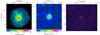 |
Fig. 2. Multiwavelengths maps of A1689. Left: XMM-Newton count map in the [0.7–1.2] keV. Middle: Planck + ACT Compton-y map. Right: Subaru Suprime-Cam image (V band). |
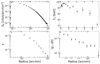 |
Fig. 3. A1689 radial profiles: upper left: X-ray surface brightness (XMM-Newton); upper right: X-ray spectroscopic temperatures (XMM Newton); lower left: SZ Compton y (Planck + ACT); lower right: Mean tangential shear (Subaru Suprime-Cam and CFHT MegaPrime/MegaCam). All of these 1D profiles will be used as inputs separately for single-probe analysis, or together for our joint multiprobe analysis. |
To derive the temperature profile we extracted spectra in 15 concentric annuli around the X-ray peak, ensuring a roughly constant signal-to-noise ratio in each radial bin. In each region and for each camera, we extracted a spectrum from the observation and the corresponding response matrix (RMF) and ancillary file (ARF) as well as a spectrum of the particle background component, with the tools mos/pn-spectra and mos/pn-back. With the same tools, we also extract a spectrum from an external annulus between 10.6′ and the edge of the field-of-view, that we use to estimate the sky background components. As described in detail in Rossetti et al. (2024), we build a model of all the background components (quiescent particle background, cosmic X-ray background, Galactic halo, local hot bubble, and residual soft protons) for each region. We then jointly fit the MOS1, MOS2, and pn spectra using the APEC model (Smith et al. 2001) in a Bayesian MCMC framework, treating the parameters of the background model as priors to derive the temperature, metal abundance and normalization of the ICM. The temperature profile is shown in the top-right panel of Fig. 3. In each radial bin, the central value is derived as the mean of the posterior distribution of temperature values, while the error bars represent the 68% confidence interval.
3.2. Sunyaev-Zel’dovich effect
The Sunyaev–Zel’dovich Compton y parameter map (middle panel of Fig. 2) used in this work combines data from the Atacama Cosmology Telescope (ACT) and Planck with 1.6 arcmin full-width half-maximum beam size, similar to the data presented in Kim et al. (2024). Specifically, the component-separated maps3 from the ACT data release 6 (DR6) observed at three frequency bands (90, 150, and 220 GHz) were utilized, providing a lower rms noise compared to the DR4 data (see Madhavacheril et al. 2020; Coulton et al. 2023).
The Compton y parameter 1D profile shown in Fig. 3 was extracted by integrating concentric circular bins equidistant in log space up to a maximum aperture of 10 arc minutes. To estimate the noise level of the Compton-y map, equal-sized patches of the ACT maps were randomly sampled. A computed uniform background of 4.3 × 10⁻⁶ was used to infer the uncertainties of the data points in the 1D profile presented. Computing the pressure profile in the mass model framework (Eq. (18)) requires a prior on the external pressure P0. We defined the latter as a normal centered on the pressure at the maximal radius aperture radius (e.i. 10 arc minutes) as shown in Table 1. This value and its error (which is used as the standard deviation of the normal prior) are taken from the 3D Planck pressure profile, part of the official products of the CHEX-MATE consortium.
Prior distributions on the model parameters.
3.3. Weak lensing
We performed a weak-lensing analysis of A1689 using archival observations from the Subaru Suprime-Cam and CFHT MegaPrime/MegaCam instruments. These data were produced as part of the CHEX-MATE collaboration (Arnaud 2021). Full details of image reduction, photometry, and shape analysis for the AMALGAM2 sample, comprising 40 CHEX-MATE clusters, will be presented in forthcoming publications (Gavazzi et al., in prep.; Umetsu et al., in prep.). In this work, we present a concise summary of our weak-lensing analysis of A1689. Our study is based on wide-field imaging in the B, V, RC, i+, and z+ bands, obtained with Suprime-Cam on the 8.2 m Subaru Telescope.
In brief, the image processing builds on AstrOmatic software suite4. In particular, astrometric solution is based on scamp (Bertin et al. 2006; Bertin 2010) using A1689 exposures but also archival images taken during the same observing run, with a slidding window of several days around the exposures of interest so that at least 3 exposures constitute the same astrometric instrument. The typical internal accuracy is of order 15 mas using Two Micron All Sky Survey (2MASS) (Skrutskie et al. 2006). It could definitely improve further with more recent Gaia reference but we deemed it sufficient for our current purpose. SWarp is used for image coaddition (Bertin et al. 2002) after the exclusion of non-photometric exposures. The selection is also based on seeing conditions. We also build a model of the Point-Spread Function (PSF) and its spatial variations is performed with PSFEx (Bertin 2011) for all the exposures in all the bands. A PSF model is also built on the coadded frames. The recovered PSF Full Width at Half Maximum (FWHM) is found to be  ,
,  ,
,  ,
,  ,
,  , in the B, V, RC, i+, and z+ bands, respectively. Galaxy shapes were measured from the RC-band data, which provide the highest image quality within the dataset, both in terms of depth and seeing. Source ellipticities were measured using the model-fitting capabilities of SExtractor, assuming the surface brightness distribution of galaxies can be well approximated by a single Sersic profile. The accuracy of this shape measurement technique was extensively assessed in the GREAT3 challenge as part of the Amalgam team (Mandelbaum et al. 2015) and further explored in the context of the preparation of the Euclid mission (Euclid Collaboration: Martinet et al. 2019). Residual multiplicative of additive biases are thus kept well below the statistical uncertainties and the weak lensing signal expected from this cluster.
Photometric redshifts (photo-z) for individual galaxies were estimated by matching the Subaru BVRCi+z+ photometry to the 30-band photometric redshift (photo-z) catalog of the 2 deg2 COSMOS field (Laigle et al. 2016). We first degrade or perturb COSMOS2015 photometry when necessary to match the depth of our A1689 data by adding extra noise in the COSMOS2015 catalog. Then, nearest neighbors in the matched BVRCi+z+ magnitude space are used for each source in order to build a photometric redshift distribution based the 100 nearest neighbors using a fast kd-tree structure (Kennel 2004). The resulting mean, median and dispersion redshift are obtained along with a marginalized mean and standard deviation of the distance ratio β ≡ Dls/Ds. A secure selection of background galaxies is key for obtaining accurate cluster mass measurements from weak lensing. The cluster lensing signal, ⟨g+(θ)⟩, was measured from a background galaxy sample selected based on a color–color (CC) cut method. This method has been calibrated against evolutionary color tracks of galaxies and photo-z catalogs from deep multiwavelength surveys such as COSMOS (for details, see Medezinski et al. 2010, 2018). In our analysis, CC cuts were performed using BRCz+ photometry from Subaru/Suprime-Cam, which offers broad coverage across the optical wavelength range and is well-suited for cluster weak-lensing studies (e.g., Umetsu et al. 2014, 2022). These CC cuts yield a background sample of 16 428 galaxies, corresponding to a mean surface number density of ng ≈ 15 galaxies arcmin−2. For the selected background sample, we find a weighted mean of  Mpc−2 and
  .
.
In Fig. 3, we show the resulting azimuthally averaged ⟨g+(θ)⟩ profile for the cluster. The profile was measured in 11 logarithmically spaced bins spanning the radial range θ ∈ [2, 20] arcmin, corresponding to cluster-centric comoving radii of (1 + zl)Dlθ ∈ [0.3, 3.0] h−1 Mpc. The error covariance matrix for the binned ⟨g+(θi)⟩ profile is expressed as Cij = Cijshape + Cijlss, where Cijshape is the diagonal statistical uncertainty due to the shape noise and Cijlss accounts for the cosmic noise due to projected uncorrelated large scale structure (Hoekstra 2003). The components of the Clss matrix were evaluated in our fiducial WMAP9 cosmology (see, e.g., Umetsu 2020).
4. Results
4.1. Gas-only analysis
Using only the gas observables provided by the X-ray data and assuming both hydrostatic equilibrium and spherical symmetry, we used the mass model method to fit an NFW profile to the X-ray surface brightness and spectroscopic temperature profiles as shown in Fig. 4. The median and the errors of the posterior distributions of the fitted parameters (c200 and r200) as well as M200 can be found in Table 2, where this first analysis can be found under the name “1-a”. The recovered concentration c200 = 6.01 ± 0.2 and mass  are in good agreement with the earlier X-ray analysis of the Chandra data on A1689 (Peng et al. 2009).
Combined analysis posterior distributions: Median Values and 1σ uncertainties (i.e., posterior distribution between the 16th and 84th percentile).
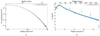 |
Fig. 4. A1689 NFW X-ray data fit in the spherical hydrostatic case. (a) X-ray brightness profile. (b) X-ray temperature profile. |
To test for consistency between the X-ray and SZ profiles, we attempted to compare the pressure profiles inferred from the two methods under the assumption of spherical symmetry. As the gNFW profile (Eq. (19)) provides a more flexible and accurate description of the pressure profile in galaxy clusters (Arnaud et al. 2010), we used the parametric forward method (see Sect. 2.3) to fit a gNFW pressure profile to the X-ray data. A mock Compton-y parameter profile was inferred by projecting the fitted pressure profile using Eq. (6). Convolving this raw mock profile with the PSF model used for the extraction of the y profile of the Planck + ACT SZ data allows a fair comparison between our X-ray inferred mock y profile and the actual Planck + ACT y profile (see Fig. 5a). We can see that the mock y profile inferred from the X-ray significantly under-predicts the observed SZ y profile. This suggests that the cluster is elongated along the LOS. Indeed, the SZ signal and the X-ray brightness increase linearly with elongation (Eq. (34)), such that the SZ-inferred pressure scale linearly with e, whereas the X-ray-inferred pressure scales with the square root of the elongation. It is thus expected that an object elongated along the LOS will exhibit a lower X-ray pressure than its SZ counterpart. We used PyMC to fit for the mean ratio of the two profiles, yPlanck + ACT = yX, mock × e1/2, accounting for the uncertainties in the SZ data. We obtain e = 1.28 ± 0.02, which significantly exceeds the value of 1.0 expected in spherical symmetry.
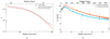 |
Fig. 5. Compton y profile and X-ray temperature profile of A1689. a) The gNFW pressure profile fitted to A1689’s X-ray data is projected and transformed into a Compton y parameter profile (dashed red) and convolved with the Planck + ACT PSF to produce a realistic mock observation (red). This profile is overplotted to the real y profile (black) extracted from Planck + ACT data. b) NFW joint X-ray and SZ analysis of A1689, X-ray temperature profile posterior distributions of 2 models: spherical and elongated (respectively in orange and light blue, model names 1-b and 1-c in Table 2). The results of the analysis as a posterior model distribution on the SZ y parameter and X-ray brightness profiles for both models can be found in the Appendix. |
Adding the Compton y parameter profile in addition to the X-ray brightness and temperature profiles, we used the mass model method to perform a joint X-ray and SZ NFW analysis. The two fitted models, spherical hydrostatic (model name 1-b) and elongated hydrostatic (model name 1-c), are shown in Fig. 5b as a fit to the X-ray temperature profile. The median and confidence interval of the best-fitting posterior distributions for both models (with e the elongation parameter in addition to c200 and r200 in the elongated case) as well as the inferred M200 values can be found in Table 2.
As anticipated from the comparison between the gNFW fit of the X-ray data and the y parameter profile (Fig. 5a), while both models successfully reproduce the X-ray brightness, the spherical model under-predicts the observed y profile (Fig. B.1). It also systematically overpredicts the X-ray temperature profile (see Fig. 5b), which implies that deviations from spherical symmetry must be taken into account to accurately model the system. Conversely, the elongated model shows elongation along the LOS at high significance (e = 1.30 ± 0.03), which allows the model to adequately fit both the X-ray and the SZ data (Fig. 5b). Our result is in agreement with Kim et al. (2024), where a 3D triaxial modeling of the cluster was fitted to 2D maps of the same data set of gas observables (X-ray and SZ), using parameterized electronic density and gas pressure profiles and without hydrostatic assumption, resulting in an equivalent elongation parameter of e = 1.37 ± 0.04 (see derivations in Appendix A).
4.2. Weak lensing only analysis
When applied to A1689, fitting our numerical model of the weak lensing signal leads to discrepant results with the gas analysis. Assuming spherical symmetry, we fitted the mean tangential shear profile of A1689 by projecting an NFW density profile and computing the reduced shear profile. The NFW model parameters were optimized in PyMC assuming Gaussian errors and taking the large-scale structure covariance matrix into account (see Sect. 3.3). The posterior envelope of the mean tangential shear profile is shown in Fig. 6, where the dashed lines show the median posterior model curves. The fitted parameter values can be found in Table 2.
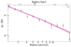 |
Fig. 6. NFW fit of the mean tangential shear profile of A1689 using the weak lensing data only and under spherical symmetry (model 2-a in Table 2). The black data points show the Subaru/HSC reduced tangential shear profile, whereas the pink curve and shaded area represent the best-fit model and 68% error envelope. |
The very steep tangential shear profile of A1689 leads the analysis to very high concentration ( ). The inferred mass (
 ) exceeds the mass inferred from the gas-only analysis (see model 2-a in Table 2) by 20%. These results converge towards the already well-known discrepancy between gas observables and weak lensing for this specific cluster (Umetsu & Broadhurst 2008; Peng et al. 2009). Our results are indeed in agreement with the previous weak lensing analysis of A1689 by Umetsu & Broadhurst (2008) (
 ,
,  ).
).
4.3. Joint X-ray and weak lensing analysis
As discussed in Sect. 2.3.2, jointly fitting gas and WL data requires the inclusion of a non-thermal pressure term to bridge a potential gap between WL and gas observables. The addition of non-thermal pressure allows to increase the system mass without impacting the fit to the gas observables (Eq. (22)). In this section, NFW profiles are jointly fitted to A1689 X-ray and WL data using the mass model method. We compare 6 models that exhaustively summarize all combinations of non-thermal pressure parameterizations and elongation allowed in our framework:
-
3-a: spherical hydrostatic,
-
3-b: elongated hydrostatic,
-
3-c: spherical and polytropic non-thermal pressure,
-
3-d: spherical and Angelinelli non-thermal pressure,
-
3-e: elongated and polytropic non-thermal pressure,
-
3-f: elongated and Angelinelli non-thermal pressure.
The medians and errors of the NFW fitted parameters posteriors (c200 and r200) and the corresponding enclosed mass M200 for the X-ray and weak lensing joint analysis are shown in Table 2 for all 6 models, as well as the elongation e and the non-thermal to thermal pressure ratio  (see Eq. (23)) when it applies. The ratio
  was picked as a representative quantity of the non-thermal pressure to offer a fair comparison regardless of the parameterization. The radial distance
  being covered by the entirety of the dataset indeed offers a good level of constraints while being at sufficiently large radii to expect an important contribution of the non-thermal pressure to the total pressure (Angelinelli et al. 2020; Gianfagna et al. 2021; Nelson et al. 2014).
In Fig. 7a we show all 6 posterior model envelopes for the joint X-ray and WL NFW analysis of A1689 as a fit to the mean tangential shear. The dashed lines show the median posterior model curves. The results of the analysis, displayed as the envelopes of the X-ray gas observables, are shown in Fig. B.2. The X-ray brightness SX and temperature TX profiles are always correctly reproduced by all models. The high statistical power of the X-ray data as compared to the weak lensing signal allows X-rays to drive the fit in the case where the model cannot provide a good fit to both, as shown by the simple spherical hydrostatic model in orange (model 3-a). Indeed, while failing at reproducing the weak lensing signal, it still provides a good prediction of the X-ray data (see Fig. B.2). By systematically underpredicting the shear, and similarly to the conclusion made after our X-ray and SZ joint fit in the previous section, model 3-a shows the limitation of the spherical hydrostatic NFW. On the other hand, either the non-thermal pressure – independently of the chosen model – or the elongation, as well as their combination, reproduces the shear signal efficiently, while keeping a similarly good fit to the X-ray data.
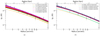 |
Fig. 7. A1689 NFW joint analysis, fit to the tangential shear profile (black points). Corresponding fits to gas observables can be found in appendix. a) Joint X-ray and WL analysis results. X-ray 1D profiles (surface brightness and temperatures) as well as the tangential shear profile are fitted jointly for every PNT (Angelinelli or polytropic parameterization) and elongation combination (models 3-a through 3-f; see Sect. 4.3 and Table 2). b) joint X-ray, SZ, and WL analysis results (see Sect. 4.4). All gas observable profiles (SX, TX, Compton y) are fitted jointly with the tangential shear profile. The three joint X-ray, SZ, and WL results shown here include the elongation parameter (i.e., elongated models) and are either not integrating any non-thermal pressure (4-a hydrostatic; cyan) or one of our two models (4-b polytropic, red; 4-c Angelinelli, purple). We also display the simple joint X-ray and WL joint analysis (3-a; orange) for a visual comparison with the spherical case. |
In this joint X-ray and WL analysis, the non-thermal pressure and elongation play a very similar role. By shifting the reconstructed shear up, these two parameters allow the model to fit both the weak lensing and the X-ray data. As a direct consequence, elongation and non-thermal pressure are here strongly anti-correlated. This is illustrated for the polytropic parameterization of the non-thermal pressure in Fig. 8a, showing the model 3-e corner plot: non-thermal pressure to total pressure ratio αNT versus the elongation parameter. The same results are observed with the Angelinelli parameterization (model 3-f) in Fig. B.3a.
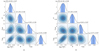 |
Fig. 8. Corner plots of the main model parameters for the NFW joint analysis of A1689 for the polytropic non-thermal pressure model with elongation (Eq. (25)). The displayed model parameters are the non-thermal pressure ratio at a radius of 0.5r200 (αNT(0.5r200)), the LOS elongation e, the concentration c200, and the overdensity radius r200 (in Mpc). Panel (a) shows the corner plot for the joint X-ray and WL analysis (model 3-e), whereas panel (b) shows the posteriors for the full joint X-ray, SZ, and WL joint analysis (model 4-b). |
We note that all considered models imply a concentration in the range 6–8, which is much lower than the concentration retrieved in the WL-only case (see Sect. 4.2). The addition of the X-ray data brings strong constraints on the shape of the underlying mass profile, which drives the concentration towards a lower and closer to the concentration-mass relation for such a massive halo.
4.4. Full NFW X-ray, SZ, and weak lensing joint analysis: non-thermal pressure parameterization comparison
As shown by comparing the projected X-ray inferred pressure profile to the SZ data and by doing the joint X-ray and SZ mass model analysis, the pressure profiles inferred from the X-ray and the SZ data have a different LOS dependency (see Sect. 4.1). As a direct consequence, the elongation parameter e propagates differently to these two observables, and fitting them jointly puts a tight constraint on the elongation parameter e. Applying our framework to the entire data set (X-ray, SZ, and weak lensing), we therefore only consider the elongated scenario and compare three different models assuming the NFW mass model:
-
4-a: elongated hydrostatic,
-
4-b: elongated and polytropic non-thermal pressure,
-
4-c: elongated and Angelinelli non-thermal pressure.
The results of the optimization for the three cases above are provided in Table 2. The fits to the tangential shear modeling of models 4-a, 4-b and 4-c are displayed in Fig. 7b, whereas the corresponding fits to the gas observables can be found in Fig. B.4. While the X-ray and SZ gas observables are well-fitted by all models without significant differences, the absence of non-thermal pressure (model 4-a) results in a systematic under-prediction of the weak lensing signal. On the other hand, the two models featuring non-thermal pressure support (models 4-b and 4-c) successfully reproduce all the profiles of the data set.
The corner plot shown in in Fig. 8b displays the posterior distribution of the elongation parameter, the non-thermal pressure ratio αNT, the NFW concentration and r200 for the polytropic parameterization (model 4-b). Jointly fitting the SZ data together with the X-ray and WL data allowed to successfully lift the degeneracy between non-thermal pressure and elongation, as compared with the previous X-ray and WL joint analysis (model 3-e; see Fig. 8a). We obtain the same results for the Angelinelli parameterization of the non-thermal pressure, as shown in Appendix Fig. B.3b. Compared to the joint X-ray and WL analysis (Sect. 4.3), adding the SZ data to the joint analysis results in a much tighter constraint on the elongation parameter. Consequently, the elongation parameter remains very stable despite changes in the non-thermal pressure parameterization, as its median posterior values, e = 1.30 ± 0.03 remain unchanged for every model (4-a, 4-b and 4-c), and consistent with our gas-only analysis (Sect. 4.1) and our previous results considering X-ray and SZ data in a full triaxial model (Kim et al. 2024).
As a consequence of the tight constraint set by the addition of the SZ data on the LOS elongation, deviations from spherical symmetry alone cannot reconcile the gas observables with the measured weak lensing signal (see model 4-a in Fig. 7b). Non-thermal pressure is now the only parameter of our framework that remains free to boost the weak lensing signal by increasing the mass of the system without impacting on the gas observables. Therefore, in the case where high-quality constraints on X-ray, WL, and SZ signals can be obtained, the degeneracy between LOS elongation and non-thermal pressure can be broken and the two parameters can be determined independently (see Fig. 8b). The non-thermal pressure at  respectively converges to ∼30 − 40% for the polytropic and Angelinelli parameterizations, while keeping a high level of agreement with each other.
The best-fitting mass model retrieved from the full analysis is fully consistent between the two non-thermal pressure parameterizations. We retrieve a concentration of ∼7 and a total spherical mass M200 = 1.76 × 10¹⁵ M⊙ (with the polytropic parameterization, model 4-b) and M200 = 1.88 × 10¹⁵ M⊙ (with the Angelinelli parameterization, model 4-c) correcting for LOS elongation. Given the scatter of ∼40% in the concentration-mass relation (e.g., Diemer & Kravtsov 2015; Klypin et al. 2016), the fitted concentration better agrees with the expected values in ΛCDM than the value of ∼15 retrieved from the WL-only analysis (see Sect. 4.2).
5. Discussion
5.1. Pressure profiles
Unlike the case of the joint X-ray and WL analysis (Sect. 4.3), our multiprobe approach, which combines X-ray, SZ, and WL data (Sect. 4.4) allows us to break the degeneracy between non-thermal pressure and LOS elongation when comparing mass reconstructions from the ICM and weak gravitational lensing. Our constraints on the two non-thermal pressure parameterizations are of comparable quality. This outcome highlights the robustness of our modeling and supports the polytropic model by bringing its constraints in line with those of the Angelinelli parameterization.
The recovered pressure profiles are presented in Fig. 9. The left panel illustrates the comparison between the thermal and non-thermal pressure profiles and the total pressure derived from the mass model (Eq. (22)). At r500, the Angelinelli and Polytropic parameterizations indicate non-thermal pressure fractions of approximately and αNT ≈ 40%. These values position A1689 among clusters with significant non-thermal pressure support, notably exceeding the 20% levels predicted by hydrodynamical simulations (e.g., Rasia et al. 2006; Lau et al. 2009; Nelson et al. 2014; Biffi et al. 2016; Angelinelli et al. 2020; Gianfagna et al. 2023) and the even lower level reported on a set of 12 clusters of the X-COP sample (Dupourqué et al. 2023) and 64 CHEX-MATE clusters (Dupourqué et al. 2024), on which the average non-thermal pressure support at r500 was found to be not higher than 10%.
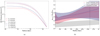 |
Fig. 9. a) Pressure profiles inferred from the A1689 NFW full joint analysis (X-ray, SZ, and WL) of both the polytropic and Angelinelli parameterizations. b) PNT/PTOT ratio for both parameterizations. The grey shaded region denotes the 1σ envelope of the non-thermal pressure profiles derived from 20 simulated clusters in Angelinelli et al. (2020), which were used to inform our prior distributions. The dashed black line marks the radius r500. The radii considered here are the 3D averaged radii. |
Nonetheless, the envelopes of αNT, shown in the right panel of Fig. 9, remain broadly consistent with simulation predictions. This aligns with findings by Morandi et al. (2011), who reported a 20% non-thermal pressure fraction in A1689 (under the assumption that αNT is constant with radius). Additionally, our results agree closely with Umetsu et al. (2015), who similarly reported a non-thermal pressure contribution reaching ∼40% at 0.9 Mpc.
Both non-thermal pressure fraction profiles show a slight increase with radius, this behavior is expected from numerical simulations (Rasia et al. 2006; Lau et al. 2009; Pearce et al. 2019; Angelinelli et al. 2020), although with significant differences from one system to another. While our results are in qualitative agreement with this prediction, application of our technique to a larger sample of clusters is needed to study the shape of the mean non-thermal pressure profile, as done for the CLASH sample (Sayers et al. 2021).
5.2. Einasto density profile
Using our multi-observable framework, we compare the results of our mass modeling between the NFW parameterization used so far to the results obtained with the Einasto density profile. We applied our reconstruction scheme to the full dataset (joint X-ray, SZ, and WL) with the polytropic non-thermal pressure parameterization and allowing for elongation (model 4-d in Table 2). The posterior distributions of the fit with the Einasto mass model are shown in Appendix Fig. B.5. Comparing the resulting mass model to its equivalent NFW joint X-ray, SZ, and WL multiprobe analysis with polytropic PNT and ellipticity (model 4-b; see the fit to the shear in Fig. 7b and to the gas observables in Fig. B.4), we can see that the Einasto and NFW density profiles provide an equally good fit to the weak lensing data and the gas observables, without significant differences.
The median NFW parameters (c200 and r200) align well with their counterparts derived from the Einasto full joint analysis, as presented in Table 2, where the Einasto concentration is inferred through the relation c200 = r200/rs. This agreement is anticipated, considering our Einasto analysis yields a value of the shape parameter α = 0.21 ± 0.03, when equivalence with the NFW parameterization is expected for α ∼ 0.2 (Dutton & Macciò 2014). Moreover, Eckert et al. (2022b) measured a mean value of α = 0.19 ± 0.03 with X-ray and SZ data on 12 massive clusters of the XMM-Newton Cluster Outskirts Project. Our best fit for the Einasto index therefore agrees with the expectations from the CDM paradigm (e.g., Navarro et al. 2004; Ludlow et al. 2016; Brown et al. 2020).
We compared our Einasto multiprobe analysis to a fit to the weak lensing data only using the same model. The WL-only fit to the shear profile is shown in Appendix Fig. B.5d. In Fig. 10 we show the posterior distributions on the Einasto index α for the multiprobe analysis and the WL data alone. For comparison, we also show the prior distribution on the Einasto shape parameter. The weak lensing only analysis does not add much constraint on the shape parameter, as the posterior distribution is nearly identical to the prior. Conversely, the joint analysis allows us to constrain the Einasto shape parameter α, as shown by the narrower posterior distribution and errors (Table 2), where we can see that the posterior distribution on α significantly pulls away from the prior. The addition of the X-ray and SZ data thus allows us to add further constraints on the shape of the DM density profile and extend beyond the NFW paradigm, which is beyond the reach of WL data even when high-quality data are available. Application of our technique to larger cluster samples will allow us to test CDM predictions on the internal structure of DM halos and provide important constraints on alternative DM scenarios such as self-interacting DM (Robertson et al. 2021; Eckert et al. 2022b).
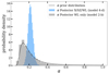 |
Fig. 10. Einasto shape parameter α prior distribution over-plotted with its posterior distributions in two cases: weak lensing only analysis (model 2-b) and full joint analysis (X-ray, SZ, and WL joint analysis with elongation and polytropic non-thermal pressure support, model 4-d). |
5.3. Successes and limitations of the model
The LOS elongation recovered thanks to our modeling shows very good agreement with Kim et al. (2024), where a full triaxial modeling of the cluster was carried out. The authors showed that A1689 is highly elliptical, and almost perfectly aligned with the LOS. This configuration explains the lower concentrations and masses inferred by the gas analysis of A1689 with respect to the lensing analysis, which shows a high lensing power and a large Einstein radius. Indeed, previous strong lensing analyses (Broadhurst et al. 2005) measured θE ∼ 50″ for the Einstein radius, which we can use as an independent test for our reconstruction. The expected Einstein radius can be predicted by our model by computing the radius θE within which the mean enclosed surface mass density equals the critical surface mass density. Assuming a mean source redshift zs = 2, from our WL-only analysis (model 2-a) we estimate  arcseconds, whereas from the full model we infer
  arcseconds (models 4-b and 4-c). Thus, the Einstein radius predicted by our model is in excellent agreement with the measured Einstein radius. Since it accounts only for LOS elongation, our model does not probe a full triaxial geometry. The projection of the cluster in the plane of the sky is assumed to be circular or circularized through other means (e.g., azimuthal median). Thanks to the almost perfect alignment between the major axis and the LOS, A1689 is well suited for this analysis, which leads to an excellent agreement between the results obtained with this technique and the results of a full triaxial analysis (Morandi et al. 2011; Sereno et al. 2012; Umetsu et al. 2015; Kim et al. 2024). Our results show that the main results of a full triaxial analysis can be mostly replicated with the addition of a single elongation parameter, which makes the model more stable numerically. On the other hand, our implementation of the underlying mass model is fully numerical, such that our framework is well suited for the study of extensions to the NFW mass model such as the Einasto model (see Sect. 5.2).
As shown in Sects. 4.3 and 4.4 and Fig. 8b, the addition of SZ data allows our framework to break the degeneracy between non-thermal pressure and LOS elongation. To further test this, we used the posterior predictive distributions of models 4-b and 4-c (our full multiprobe and elongated modeling approaches, implementing the polytropic and Angelinelli parameterizations of non-thermal pressure, respectively) to generate synthetic realizations of observables. Specifically, we drew 4 × 2 sets of profiles, each consisting of SX, TX, y, and g+. We then fit these synthetic profiles using two different setups: (i) an X-ray and Weak Lensing (X/WL) analysis, and (ii) a full joint X-ray, SZ, and WL (X/SZ/WL) analysis, where the latter incorporates SZ constraints. This allowed us to isolate the role of SZ data in breaking the degeneracy between elongation and non-thermal pressure. Fig. B.6 presents a comparison of the constraints on  and e obtained from both analyses. The recovered values from the joint X-ray and WL and joint X-ray, SZ, and WL are compared against the “true” posterior distributions of
  and e inferred from models 4-b and 4-c. In the absence of SZ data, the recovered elongation is biased low due to the prior. Adding SZ data, however, enables a successful recovery of A1689’s median posterior distributions for both the elongation parameter e and non-thermal pressure
  , reducing their errors by factors of 5.5 and 1.4, respectively. The addition of the two parameters, LOS elongation and non-thermal pressure, allows us to reconcile, respectively, the X-ray and SZ observations, and the combined X-ray and SZ data with weak lensing measurements. In Fig. B.7, we present the histograms of the normalized residuals from the NFW fits to A1689 for the joint X-ray and SZ analysis with and without the inclusion of elongation (models 1-b and 1-c), and for the full joint X-ray, SZ, and WL analysis with and without non-thermal pressure (models 4-a and 4-b). A comparison between models 1-b and 1-c, as well as between 4-a and 4-b, clearly demonstrates that the addition of elongation and non-thermal pressure significantly improves the quality of the fits, both in terms of total and individual observables. Therefore, we rely on the availability of high-quality observations in X-rays, SZ and weak lensing. To the present day, the available multiwavelength data on A1689 are unrivalled, which makes this system the ideal candidate to validate our framework. However, upcoming large SZ (ACT, SPT) and weak lensing surveys (e.g., Euclid, Rubin) will bring datasets of similar quality for an increasing number of systems, which will allow us to study the distribution of three-dimensional cluster shapes and non-thermal pressure in sizable cluster samples.
As demonstrated by comparing our joint X-ray and SZ and joint X-ray, SZ, and WL analysis, the main source of constraint on the LOS elongation parameter e in our model comes from the ratio between the SZ and X-ray pressure profiles (De Filippis et al. 2005; Sereno et al. 2006; Bourdin et al. 2017; Kozmanyan et al. 2019). This  ratio also depends on the Hubble constant, and scaling with h0.5 (Kozmanyan et al. 2019; Ettori et al. 2020). Considering h values ranging from 0.68 to 0.73, this results in an additional 3.6% uncertainty on the elongation parameter e.
Lau et al. (2011) demonstrated that the gas distribution traces the shape of the gravitational potential, which usually differs from that of the DM distribution. As a result, the ellipticity estimated by our model is that of the gravitational potential rather than that of the mass distribution. In a triaxial geometry, the gravitational potential is usually more spherical than the underlying mass distribution, as it results from the point-to-point potential averaged over the entire system (Sereno 2007; Kawahara 2010). As a result, our assumption that the gas and DM are co-aligned may be overly simplistic. We showed in our full joint X-ray, SZ, and WL multiprobe analysis that adding the weak lensing data does not impact the recovered LOS elongation, but instead constrains the non-thermal pressure. In case the ellipticity of the DM is larger than that of the potential (and, hence, the gas), the shear profile should be more affected by LOS elongation than the corresponding gas observables (Eq. (31)), such that the total mass and, in turn, the non-thermal pressure should be slightly lower than reported in this paper. Future versions of our pipeline will include a self-consistent treatment of LOS elongation on the gas and the DM.
6. Conclusion
In this paper, we introduced a new framework to reconstruct the shape of galaxy cluster mass profiles and non-thermal pressure support from the combination of X-ray, SZ, and WL data. We implemented a weak lensing module to the already existing code hydromass (Eckert et al. 2022a), thus making it possible to fit tangential shear profiles jointly with X-ray (temperature and surface brightness profiles) and SZ (Compton y profile) data. To account for possible differences between the three observables, we introduced a LOS elongation parameter, e, and non-thermal pressure support using two parameterizations (polytropic and Angelinelli).
When we applied our multiprobe framework to Abell 1689, we successfully fitted a density profile (NFW and Einasto) and were able to reproduce the observed profiles of X-ray surface brightness and temperature, Compton-y parameter, and mean tangential shear within a common framework. We showed that A1689 is significantly elongated along the LOS, with the fitted elongation, e, being significantly different from unity with an uncertainty of only a few percent (e = 1.30 ± 0.03 from the full multiprobe analysis, accounting for non-thermal pressure; models 4-b and 4-c). When we fit X-ray and WL data only, the contribution of non-thermal pressure and LOS elongation was highly degenerate. The degeneracy can be broken by including the SZ data (see Fig. 8b). Using the full dataset, our framework is able to recover the non-thermal pressure support, which constitutes the main source of hydrostatic bias when comparing X-ray galaxy cluster masses to weak lensing masses. The non-thermal pressure profiles obtained from the two parameterizations introduced in this work (polytropic and Angelinelli, see Sect. 2.3.2) are consistent with one another, and yield a substantial non-thermal pressure support of ∼40% at r500.
Our forward modeling approach of all the available observables (X-ray surface brightness and temperatures, Compton y, and mean tangential shear profiles) is fully numerical. As a result, our framework is able to perform a similar reconstruction for any chosen density profile and move beyond the assumption of an NFW density profile. In the NFW case, we showed that the very high concentration inferred from WL data only under the assumption of spherical symmetry (c200 ∼ 15, see Sect. 4.2) comes down to the more reasonable value of ∼7 when the gas observables are included in the model (see Table 2). When we fit the data with the Einasto model instead of NFW, we showed that both models provide a good fit to the A1689 dataset. Our multiprobe framework is able to constrain the Einasto shape parameter α = 0.21 ± 0.03, whereas in the WL-only analysis the parameter does not pull away from the prior. Applying our framework to a larger sample of galaxy clusters such as CHEX-MATE (Arnaud 2021), for which we find that 18 clusters (including A1689) are covered by ACT DR6 and part of the AMALGAM2 sample, will allow us to determine the shape of DM mass profiles, constrain the three-dimensional shape of galaxy clusters, and estimate the impact of non-thermal pressure support across the population.
Acknowledgments
Based on observations obtained with XMM-Newton, an ESA science mission with instruments and contributions directly funded by ESA Member States and NASA. DE acknowledges support from the Swiss National Science Foundation (SNSF) under grant agreement 200021_212576. AG, JS, and HS were supported by NASA Astrophysics Data Analysis Program (ADAP) Grant 80NSSC21K1571. SE, MR, FG, IB, VG, HB, FDL, and PM acknowledge the financial contribution from the contracts Prin-MUR 2022, supported by Next Generation EU (n.20227RNLY3 The concordance cosmological model: stress-tests with galaxy clusters), ASI-INAF Athena 2019-27-HH.0, “Attività di Studio per la comunità scientifica di Astrofisica delle Alte Energie e Fisica Astroparticellare” (Accordo Attuativo ASI-INAF n. 2017-14-H.0). EP acknowledges the support of the French Agence Nationale de la Recherche (ANR), under grant ANR-22-CE31-0010 (project BATMAN). RC acknowledges financial support from the INAF grant 2023 “Testing the origin of giant radio halos with joint LOFAR” (1.05.23.05.11). BJM acknowledges support from STFC grant ST/V000454/1. MG acknowledges support from the ERC Consolidator Grant BlackHoleWeather (101086804). GWP acknowledges long-term support from CNES, the French space agency. This research was supported by the International Space Science Institute (ISSI) in Bern, through ISSI International Team project #565 (multiwavelength Studies of the Culmination of Structure Formation in the Universe).
References
- Allen, S. W., Evrard, A. E., & Mantz, A. B. 2011, ARA&A, 49, 409 [Google Scholar]
- Ameglio, S., Borgani, S., Pierpaoli, E., & Dolag, K. 2007, MNRAS, 382, 397 [NASA ADS] [CrossRef] [Google Scholar]
- Andersson, K. E., & Madejski, G. M. 2004, ApJ, 607, 190 [Google Scholar]
- Angelinelli, M., Vazza, F., Giocoli, C., et al. 2020, MNRAS, 495, 864 [NASA ADS] [CrossRef] [Google Scholar]
- Arnaud, M., Pratt, G. W., Piffaretti, R., et al. 2010, A&A, 517, A92 [CrossRef] [EDP Sciences] [Google Scholar]
- Asplund, M., Grevesse, N., Sauval, A. J., & Scott, P. 2009, ARA&A, 47, 481 [NASA ADS] [CrossRef] [Google Scholar]
- Barnes, D. J., Vogelsberger, M., Pearce, F. A., et al. 2021, MNRAS, 506, 2533 [NASA ADS] [CrossRef] [Google Scholar]
- Bartalucci, I., Molendi, S., Rasia, E., et al. 2023, A&A, 674, A179 [NASA ADS] [CrossRef] [EDP Sciences] [Google Scholar]
- Bartelmann, M., & Schneider, P. 2001, Phys. Rep., 340, 291 [Google Scholar]
- Bennett, J. S., & Sijacki, D. 2022, MNRAS, 514, 313 [CrossRef] [Google Scholar]
- Bertin, E. 2006, in Astronomical Data Analysis Software and Systems XV, eds. C. Gabriel, C. Arviset, D. Ponz, & S. Enrique, ASP Conf. Ser., 351, 112 [Google Scholar]
- Bertin, E. 2010, SCAMP: Automatic Astrometric and PhotometricCalibration, Astrophysics Source Code Library [record ascl:1010.063] [Google Scholar]
- Bertin, E. 2011, in Astronomical Data Analysis Software and Systems XX, eds. I. N. Evans, A. Accomazzi, D. J. Mink, & A. H. Rots, ASP Conf. Ser., 442, 435 [Google Scholar]
- Bertin, E., Mellier, Y., Radovich, M., et al. 2002, in Astronomical Data Analysis Software and Systems XI, eds. D. A. Bohlender, D. Durand, & T. H. Handley, ASP Conf. Ser., 281, 228 [NASA ADS] [Google Scholar]
- Biffi, V., Borgani, S., Murante, G., et al. 2016, ApJ, 827, 112 [NASA ADS] [CrossRef] [Google Scholar]
- Bourdin, H., Mazzotta, P., Kozmanyan, A., Jones, C., & Vikhlinin, A. 2017, ApJ, 843, 72 [Google Scholar]
- Broadhurst, T., Benitez, N., Coe, D., et al. 2005, ApJ, 621, 53 [Google Scholar]
- Brown, S. T., McCarthy, I. G., Diemer, B., et al. 2020, MNRAS, 495, 4994 [NASA ADS] [CrossRef] [Google Scholar]
- Bulbul, G. E., Hasler, N., Bonamente, M., & Joy, M. 2010, ApJ, 720, 1038 [NASA ADS] [CrossRef] [Google Scholar]
- Bullock, J. S., Kolatt, T. S., Sigad, Y., et al. 2001, MNRAS, 321, 559 [Google Scholar]
- Capelo, P. R., Coppi, P. S., & Natarajan, P. 2012, MNRAS, 422, 686 [NASA ADS] [CrossRef] [Google Scholar]
- Cappellari, M., & Copin, Y. 2003, MNRAS, 342, 345 [Google Scholar]
- Chen, K.-F., Oguri, M., Lin, Y.-T., & Miyazaki, S. 2020, ApJ, 891, 139 [NASA ADS] [CrossRef] [Google Scholar]
- CHEX-MATE Collaboration (Arnaud, M., et al.) 2021, A&A, 650, A104 [NASA ADS] [CrossRef] [EDP Sciences] [Google Scholar]
- Chiu, I., Mohr, J. J., McDonald, M., et al. 2018a, MNRAS, 478, 3072 [Google Scholar]
- Chiu, I. N., Umetsu, K., Sereno, M., et al. 2018b, ApJ, 860, 126 [NASA ADS] [CrossRef] [Google Scholar]
- Coulton, W. R., Madhavacheril, M. S., Duivenvoorden, A. J., et al. 2023, arXiv e-prints [arXiv:2307.01258] [Google Scholar]
- Cuciti, V., Cassano, R., Brunetti, G., et al. 2015, A&A, 580, A97 [CrossRef] [EDP Sciences] [Google Scholar]
- De Filippis, E., Sereno, M., Bautz, M. W., & Longo, G. 2005, ApJ, 625, 108 [NASA ADS] [CrossRef] [Google Scholar]
- Despali, G., Giocoli, C., & Tormen, G. 2014, MNRAS, 443, 3208 [Google Scholar]
- Diemer, B., & Kravtsov, A. V. 2015, ApJ, 799, 108 [Google Scholar]
- Dupourqué, S., Clerc, N., Pointecouteau, E., et al. 2023, A&A, 673, A91 [NASA ADS] [CrossRef] [EDP Sciences] [Google Scholar]
- Dupourqué, S., Clerc, N., Pointecouteau, E., et al. 2024, A&A, 687, A58 [NASA ADS] [CrossRef] [EDP Sciences] [Google Scholar]
- Dutton, A. A., & Macciò, A. V. 2014, MNRAS, 441, 3359 [Google Scholar]
- Eckert, D., Roncarelli, M., Ettori, S., et al. 2015, MNRAS, 447, 2198 [Google Scholar]
- Eckert, D., Ghirardini, V., Ettori, S., et al. 2019, A&A, 621, A40 [NASA ADS] [CrossRef] [EDP Sciences] [Google Scholar]
- Eckert, D., Finoguenov, A., Ghirardini, V., et al. 2020, Open J. Astrophys., 3, 12 [NASA ADS] [CrossRef] [Google Scholar]
- Eckert, D., Ettori, S., Pointecouteau, E., van der Burg, R. F. J., & Loubser, S. I. 2022a, A&A, 662, A123 [NASA ADS] [CrossRef] [EDP Sciences] [Google Scholar]
- Eckert, D., Ettori, S., Robertson, A., et al. 2022b, A&A, 666, A41 [NASA ADS] [CrossRef] [EDP Sciences] [Google Scholar]
- Einasto, J. 1965, Trudy Astrofizicheskogo Instituta Alma-Ata, 5, 87 [NASA ADS] [Google Scholar]
- Ettori, S., & Eckert, D. 2022, A&A, 657, L1 [NASA ADS] [CrossRef] [EDP Sciences] [Google Scholar]
- Ettori, S., Gastaldello, F., Leccardi, A., et al. 2011, A&A, 526, C1 [NASA ADS] [CrossRef] [EDP Sciences] [Google Scholar]
- Ettori, S., Ghirardini, V., Eckert, D., et al. 2019, A&A, 621, A39 [NASA ADS] [CrossRef] [EDP Sciences] [Google Scholar]
- Ettori, S., Ghirardini, V., & Eckert, D. 2020, Astron. Nachr., 341, 210 [NASA ADS] [CrossRef] [Google Scholar]
- Ettori, S., Lovisari, L., & Eckert, D. 2023, A&A, 669, A133 [NASA ADS] [CrossRef] [EDP Sciences] [Google Scholar]
- Euclid Collaboration (Martinet, N., et al.) 2019, A&A, 627, A59 [NASA ADS] [CrossRef] [EDP Sciences] [Google Scholar]
- Euclid Collaboration (Giocoli, C., et al.) 2024, A&A, 681, A67 [NASA ADS] [CrossRef] [EDP Sciences] [Google Scholar]
- Gavazzi, R. 2005, A&A, 443, 793 [NASA ADS] [CrossRef] [EDP Sciences] [Google Scholar]
- Ghirardini, V., Ettori, S., Eckert, D., & Molendi, S. 2019, A&A, 627, A19 [NASA ADS] [CrossRef] [EDP Sciences] [Google Scholar]
- Gianfagna, G., De Petris, M., Yepes, G., et al. 2021, MNRAS, 502, 5115 [NASA ADS] [CrossRef] [Google Scholar]
- Gianfagna, G., Rasia, E., Cui, W., et al. 2023, MNRAS, 518, 4238 [Google Scholar]
- Gonzalez, A. H., Sivanandam, S., Zabludoff, A. I., & Zaritsky, D. 2013, ApJ, 778, 14 [Google Scholar]
- Grandis, S., Bocquet, S., Mohr, J. J., Klein, M., & Dolag, K. 2021, MNRAS, 507, 5671 [NASA ADS] [CrossRef] [Google Scholar]
- Hennawi, J. F., Dalal, N., Bode, P., & Ostriker, J. P. 2007, ApJ, 654, 714 [NASA ADS] [CrossRef] [Google Scholar]
- Herbonnet, R., Sifón, C., Hoekstra, H., et al. 2020, MNRAS, 497, 4684 [NASA ADS] [CrossRef] [Google Scholar]
- Hinshaw, G., Larson, D., Komatsu, E., et al. 2013, ApJS, 208, 19 [Google Scholar]
- Hoekstra, H. 2003, MNRAS, 339, 1155 [NASA ADS] [CrossRef] [Google Scholar]
- Hoekstra, H., Bartelmann, M., Dahle, H., et al. 2013, Space Sci. Rev., 177, 75 [NASA ADS] [CrossRef] [Google Scholar]
- Hoekstra, H., Herbonnet, R., Muzzin, A., et al. 2015, MNRAS, 449, 685 [NASA ADS] [CrossRef] [Google Scholar]
- Hoffman, M. D., & Gelman, A. 2011, arXiv e-prints [arXiv:1111.4246] [Google Scholar]
- Kawahara, H. 2010, ApJ, 719, 1926 [Google Scholar]
- Kennel, M. B. 2004, arXiv e-prints [arXiv:physics/0408067] [Google Scholar]
- Kim, J., Sayers, J., Sereno, M., et al. 2024, A&A, 686, A97 [NASA ADS] [CrossRef] [EDP Sciences] [Google Scholar]
- Klypin, A., Yepes, G., Gottlöber, S., Prada, F., & Heß, S. 2016, MNRAS, 457, 4340 [Google Scholar]
- Kneib, J.-P., & Natarajan, P. 2011, A&A Rev., 19, 47 [Google Scholar]
- Kozmanyan, A., Bourdin, H., Mazzotta, P., Rasia, E., & Sereno, M. 2019, A&A, 621, A34 [NASA ADS] [CrossRef] [EDP Sciences] [Google Scholar]
- Kravtsov, A. V., & Borgani, S. 2012, ARA&A, 50, 353 [Google Scholar]
- Kriss, G. A., Cioffi, D. F., & Canizares, C. R. 1983, ApJ, 272, 439 [Google Scholar]
- Laigle, C., McCracken, H. J., Ilbert, O., et al. 2016, ApJS, 224, 24 [Google Scholar]
- Lau, E. T., Kravtsov, A. V., & Nagai, D. 2009, ApJ, 705, 1129 [NASA ADS] [CrossRef] [Google Scholar]
- Lau, E. T., Nagai, D., Kravtsov, A. V., & Zentner, A. R. 2011, ApJ, 734, 93 [CrossRef] [Google Scholar]
- Lau, E. T., Hearin, A. P., Nagai, D., & Cappelluti, N. 2020, MNRAS, 500, 1029 [CrossRef] [Google Scholar]
- Le Brun, A. M. C., Arnaud, M., Pratt, G. W., & Teyssier, R. 2017, MNRAS, 473, L69 [Google Scholar]
- Lemze, D., Barkana, R., Broadhurst, T. J., & Rephaeli, Y. 2008, MNRAS, 386, 1092 [Google Scholar]
- Limousin, M., Morandi, A., Sereno, M., et al. 2013, Space Sci. Rev., 177, 155 [Google Scholar]
- Ludlow, A. D., Bose, S., Angulo, R. E., et al. 2016, MNRAS, 460, 1214 [Google Scholar]
- Macciò, A. V., Dutton, A. A., & van den Bosch, F. C. 2008, MNRAS, 391, 1940 [Google Scholar]
- Madhavacheril, M. S., Hill, J. C., Næss, S., et al. 2020, Phys. Rev., D, 102 [Google Scholar]
- Mandelbaum, R., Rowe, B., Armstrong, R., et al. 2015, MNRAS, 450, 2963 [Google Scholar]
- Mastromarino, C., Oppizzi, F., De Luca, F., Bourdin, H., & Mazzotta, P. 2024, A&A, 688, A76 [NASA ADS] [CrossRef] [EDP Sciences] [Google Scholar]
- Mazzotta, P., Rasia, E., Moscardini, L., & Tormen, G. 2004, MNRAS, 354, 10 [NASA ADS] [CrossRef] [Google Scholar]
- Medezinski, E., Broadhurst, T., Umetsu, K., et al. 2010, MNRAS, 405, 257 [NASA ADS] [Google Scholar]
- Medezinski, E., Battaglia, N., Umetsu, K., et al. 2017, PASJ, 70 [Google Scholar]
- Medezinski, E., Oguri, M., Nishizawa, A. J., et al. 2018, PASJ, 70, 30 [NASA ADS] [Google Scholar]
- Meneghetti, M., Rasia, E., Merten, J., et al. 2010, A&A, 514, A93 [NASA ADS] [CrossRef] [EDP Sciences] [Google Scholar]
- Miniati, F., & Beresnyak, A. 2015, Nature, 523, 59 [NASA ADS] [CrossRef] [Google Scholar]
- Morandi, A., Limousin, M., Rephaeli, Y., et al. 2011, MNRAS, 416, 2567 [NASA ADS] [CrossRef] [Google Scholar]
- Morandi, A., Limousin, M., Sayers, J., et al. 2012, MNRAS, 425, 2069 [NASA ADS] [CrossRef] [Google Scholar]
- Muñoz-Echeverría, M., Macías-Pèrez, J. F., Pratt, G. W., et al. 2023, A&A, 671, A28 [NASA ADS] [CrossRef] [EDP Sciences] [Google Scholar]
- Nagai, D., & Lau, E. T. 2011, ApJ, 731, L10 [NASA ADS] [CrossRef] [Google Scholar]
- Nagai, D., Kravtsov, A. V., & Vikhlinin, A. 2007, ApJ, 668, 1 [Google Scholar]
- Navarro, J. F., Frenk, C. S., & White, S. D. M. 1996, ApJ, 462, 563 [Google Scholar]
- Navarro, J. F., Hayashi, E., Power, C., et al. 2004, MNRAS, 349, 1039 [Google Scholar]
- Navarro, J. F., Ludlow, A., Springel, V., et al. 2009, MNRAS, 402, 21 [Google Scholar]
- Nelson, K., Lau, E. T., Nagai, D., Rudd, D. H., & Yu, L. 2014, ApJ, 782, 107 [NASA ADS] [CrossRef] [Google Scholar]
- Oguri, M., Takada, M., Umetsu, K., & Broadhurst, T. 2005, ApJ, 632, 841 [Google Scholar]
- Okabe, N., & Smith, G. P. 2016, MNRAS, 461, 3794 [Google Scholar]
- Patil, A., Huard, D., & Fonnesbeck, C. J. 2010, J. Stat. Software, 35, 1 [Google Scholar]
- Pearce, F. A., Kay, S. T., Barnes, D. J., Bower, R. G., & Schaller, M. 2019, MNRAS, 491, 1622 [Google Scholar]
- Peng, E.-H., Andersson, K., Bautz, M. W., & Garmire, G. P. 2009, ApJ, 701, 1283 [Google Scholar]
- Pointecouteau, E., & Silk, J. 2005, MNRAS, 364, 654 [NASA ADS] [CrossRef] [Google Scholar]
- Power, C., Navarro, J. F., Jenkins, A., et al. 2003, MNRAS, 338, 14 [Google Scholar]
- Pratt, G. W., Arnaud, M., Biviano, A., et al. 2019, Space Sci. Rev., 215 [CrossRef] [Google Scholar]
- Rasia, E., Ettori, S., Moscardini, L., et al. 2006, MNRAS, 369, 2013 [CrossRef] [Google Scholar]
- Rasia, E., Meneghetti, M., Martino, R., et al. 2012, New J. Phys., 14, 055018 [Google Scholar]
- Robertson, A., Massey, R., Eke, V., Schaye, J., & Theuns, T. 2021, MNRAS, 501, 4610 [NASA ADS] [CrossRef] [Google Scholar]
- Rossetti, M., & Molendi, S. 2010, A&A, 510, A83 [NASA ADS] [CrossRef] [EDP Sciences] [Google Scholar]
- Rossetti, M., Eckert, D., Gastaldello, F., et al. 2024, A&A, 686, A68 [NASA ADS] [CrossRef] [EDP Sciences] [Google Scholar]
- Sayers, J., Sereno, M., Ettori, S., et al. 2021, MNRAS, 505, 4338 [NASA ADS] [CrossRef] [Google Scholar]
- Seitz, C., & Schneider, P. 1997, A&A, 318, 687 [NASA ADS] [Google Scholar]
- Sereno, M. 2007, MNRAS, 380, 1207 [CrossRef] [Google Scholar]
- Sereno, M., & Umetsu, K. 2011, MNRAS, 416, 3187 [NASA ADS] [CrossRef] [Google Scholar]
- Sereno, M., De Filippis, E., Longo, G., & Bautz, M. W. 2006, ApJ, 645, 170 [NASA ADS] [CrossRef] [Google Scholar]
- Sereno, M., Ettori, S., & Baldi, A. 2012, MNRAS, 419, 2646 [NASA ADS] [CrossRef] [Google Scholar]
- Sereno, M., Ettori, S., Umetsu, K., & Baldi, A. 2013, MNRAS, 428, 2241 [NASA ADS] [CrossRef] [Google Scholar]
- Sereno, M., Covone, G., Izzo, L., et al. 2017a, MNRAS, 472, 1946 [Google Scholar]
- Sereno, M., Ettori, S., Meneghetti, M., et al. 2017b, MNRAS, 467, 3801 [NASA ADS] [CrossRef] [Google Scholar]
- Sereno, M., Umetsu, K., Ettori, S., et al. 2018, ApJ, 860, L4 [NASA ADS] [CrossRef] [Google Scholar]
- Skrutskie, M. F., Cutri, R. M., Stiening, R., et al. 2006, AJ, 131, 1163 [NASA ADS] [CrossRef] [Google Scholar]
- Smith, R. K., Brickhouse, N. S., Liedahl, D. A., & Raymond, J. C. 2001, ApJ, 556, L91 [Google Scholar]
- Umetsu, K. 2020, A&A Rev., 28, 7 [NASA ADS] [CrossRef] [Google Scholar]
- Umetsu, K., & Broadhurst, T. 2008, ApJ, 684, 177 [Google Scholar]
- Umetsu, K., Medezinski, E., Nonino, M., et al. 2014, ApJ, 795, 163 [NASA ADS] [CrossRef] [Google Scholar]
- Umetsu, K., Sereno, M., Medezinski, E., et al. 2015, ApJ, 806, 207 [NASA ADS] [CrossRef] [Google Scholar]
- Umetsu, K., Ueda, S., Hsieh, B.-C., et al. 2022, ApJ, 934, 169 [NASA ADS] [CrossRef] [Google Scholar]
- Vacca, V., Govoni, F., Murgia, M., et al. 2011, A&A, 535, A82 [NASA ADS] [CrossRef] [EDP Sciences] [Google Scholar]
- Vazza, F., Angelinelli, M., Jones, T. W., et al. 2018, MNRAS, 481, L120 [NASA ADS] [CrossRef] [Google Scholar]
- Vikhlinin, A., Kravtsov, A., Forman, W., et al. 2006, ApJ, 640, 691 [Google Scholar]
- von der Linden, A., Allen, M. T., Applegate, D. E., et al. 2014, MNRAS, 439, 2 [NASA ADS] [CrossRef] [Google Scholar]
- Wechsler, R. H., Bullock, J. S., Primack, J. R., Kravtsov, A. V., & Dekel, A. 2002, ApJ, 568, 52 [NASA ADS] [CrossRef] [Google Scholar]
- Wu, H.-Y., Costanzi, M., To, C.-H., et al. 2022, MNRAS, 515, 4471 [CrossRef] [Google Scholar]
Appendix A: Comparison to triaxial modeling of Kim et al. (2024)
In Kim et al. (2024), a 3D triaxial modeling of A1689 was fitted to 2D maps of the same data set of gas observables (X-ray and SZ), using parameterized electronic density and gas pressure profiles and without hydrostatic assumption. The authors used a similar data set and also inferred the line of sight elongation through comparison of X-ray and SZ data, they offer a very comparable output. The recovered elongation parameter e|| of their modeling is defined as the ratio of the size of the ellipsoid along the LOS (llos) to the major axis of the projected ellipse in the plane of the sky (lp):

To enable a direct comparison between the line-of-sight elongation parameter obtained from our circular symmetry model and the triaxial model used by Kim et al. (2024), we convert their fitted triaxial parameters (the minor-to-major and intermediate-to-major axial ratios denoted q1 and q2, inclination angle θ, and Euler angles ϕ and ψ) into a comparable elongation measure e. Here, e is defined as the ratio of the line-of-sight length of the cluster llos to leff, the effective radius of a circle with an equivalent area to that of the projected ellipse in the plane of the sky:


where qp is the minor-to-major axial ratio of the observed projected isophote. Its definition can be found in Eq. 3 of Kim et al. (2024), along with an exhaustive description of all the geometrical parameters involved in its computation. This conversion allows for a consistent comparison between the elongation derived from the full triaxial modeling with the plane of the sky circular symmetry assumption we make in our work. Kim et al. (2024) recovered a value e|| = 1.24 ± 0.03 which we convert into e = 1.37 ± 0.03.
Appendix B: Additional diagnostic plots
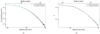 |
Fig. B.1. A1689 joint X-ray and SZ, NFW joint analysis: fits to the X-ray brightness (left) and SZ y parameter (right). |
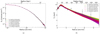 |
Fig. B.2. A1689 X-ray and WL, NFW joint analysis: fits to the X-ray observables. |
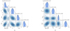 |
Fig. B.3. NFW joint analysis of A1689: corner plots featuring Angelinelli Non-thermal pressure to total pressure ratio αNT(0.5r200), los elongation e, concentration c200 and radius r200 (in Mpc). a) X-ray and WL joint analysis, b) full joint X-ray, SZ, and WL joint analysis. |
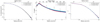 |
Fig. B.4. A1689 joint X-ray, SZ, and WL, NFW joint analysis results: fits to the gas observables. |
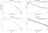 |
Fig. B.5. joint X-ray, SZ, and WL joint analysis results: total A1689 data set fitted with the Einasto density profile in the elongated case with polytropic non-thermal pressure. The mean tangential shear profile also features the result for the Weak Lensing only Einasto analysis. |
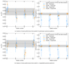 |
Fig. B.6. Comparison of the recovered values for the non-thermal pressure fraction, |


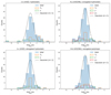 |
Fig. B.7. Comparison of the histograms of the residuals ( |

All Tables
Combined analysis posterior distributions: Median Values and 1σ uncertainties (i.e., posterior distribution between the 16th and 84th percentile).
All Figures
|
Fig. 1. Sketch of the implemented elongation correction. The sketch shows the isodensity surface of an ellipsoidal halo (blue solid curve) in the LOS (z) – plane of the sky ( |
| In the text | |
|
Fig. 2. Multiwavelengths maps of A1689. Left: XMM-Newton count map in the [0.7–1.2] keV. Middle: Planck + ACT Compton-y map. Right: Subaru Suprime-Cam image (V band). |
| In the text | |
|
Fig. 3. A1689 radial profiles: upper left: X-ray surface brightness (XMM-Newton); upper right: X-ray spectroscopic temperatures (XMM Newton); lower left: SZ Compton y (Planck + ACT); lower right: Mean tangential shear (Subaru Suprime-Cam and CFHT MegaPrime/MegaCam). All of these 1D profiles will be used as inputs separately for single-probe analysis, or together for our joint multiprobe analysis. |
| In the text | |
|
Fig. 4. A1689 NFW X-ray data fit in the spherical hydrostatic case. (a) X-ray brightness profile. (b) X-ray temperature profile. |
| In the text | |
|
Fig. 5. Compton y profile and X-ray temperature profile of A1689. a) The gNFW pressure profile fitted to A1689’s X-ray data is projected and transformed into a Compton y parameter profile (dashed red) and convolved with the Planck + ACT PSF to produce a realistic mock observation (red). This profile is overplotted to the real y profile (black) extracted from Planck + ACT data. b) NFW joint X-ray and SZ analysis of A1689, X-ray temperature profile posterior distributions of 2 models: spherical and elongated (respectively in orange and light blue, model names 1-b and 1-c in Table 2). The results of the analysis as a posterior model distribution on the SZ y parameter and X-ray brightness profiles for both models can be found in the Appendix. |
| In the text | |
|
Fig. 6. NFW fit of the mean tangential shear profile of A1689 using the weak lensing data only and under spherical symmetry (model 2-a in Table 2). The black data points show the Subaru/HSC reduced tangential shear profile, whereas the pink curve and shaded area represent the best-fit model and 68% error envelope. |
| In the text | |
|
Fig. 7. A1689 NFW joint analysis, fit to the tangential shear profile (black points). Corresponding fits to gas observables can be found in appendix. a) Joint X-ray and WL analysis results. X-ray 1D profiles (surface brightness and temperatures) as well as the tangential shear profile are fitted jointly for every PNT (Angelinelli or polytropic parameterization) and elongation combination (models 3-a through 3-f; see Sect. 4.3 and Table 2). b) joint X-ray, SZ, and WL analysis results (see Sect. 4.4). All gas observable profiles (SX, TX, Compton y) are fitted jointly with the tangential shear profile. The three joint X-ray, SZ, and WL results shown here include the elongation parameter (i.e., elongated models) and are either not integrating any non-thermal pressure (4-a hydrostatic; cyan) or one of our two models (4-b polytropic, red; 4-c Angelinelli, purple). We also display the simple joint X-ray and WL joint analysis (3-a; orange) for a visual comparison with the spherical case. |
| In the text | |
|
Fig. 8. Corner plots of the main model parameters for the NFW joint analysis of A1689 for the polytropic non-thermal pressure model with elongation (Eq. (25)). The displayed model parameters are the non-thermal pressure ratio at a radius of 0.5r200 (αNT(0.5r200)), the LOS elongation e, the concentration c200, and the overdensity radius r200 (in Mpc). Panel (a) shows the corner plot for the joint X-ray and WL analysis (model 3-e), whereas panel (b) shows the posteriors for the full joint X-ray, SZ, and WL joint analysis (model 4-b). |
| In the text | |
|
Fig. 9. a) Pressure profiles inferred from the A1689 NFW full joint analysis (X-ray, SZ, and WL) of both the polytropic and Angelinelli parameterizations. b) PNT/PTOT ratio for both parameterizations. The grey shaded region denotes the 1σ envelope of the non-thermal pressure profiles derived from 20 simulated clusters in Angelinelli et al. (2020), which were used to inform our prior distributions. The dashed black line marks the radius r500. The radii considered here are the 3D averaged radii. |
| In the text | |
|
Fig. 10. Einasto shape parameter α prior distribution over-plotted with its posterior distributions in two cases: weak lensing only analysis (model 2-b) and full joint analysis (X-ray, SZ, and WL joint analysis with elongation and polytropic non-thermal pressure support, model 4-d). |
| In the text | |
|
Fig. B.1. A1689 joint X-ray and SZ, NFW joint analysis: fits to the X-ray brightness (left) and SZ y parameter (right). |
| In the text | |
|
Fig. B.2. A1689 X-ray and WL, NFW joint analysis: fits to the X-ray observables. |
| In the text | |
|
Fig. B.3. NFW joint analysis of A1689: corner plots featuring Angelinelli Non-thermal pressure to total pressure ratio αNT(0.5r200), los elongation e, concentration c200 and radius r200 (in Mpc). a) X-ray and WL joint analysis, b) full joint X-ray, SZ, and WL joint analysis. |
| In the text | |
|
Fig. B.4. A1689 joint X-ray, SZ, and WL, NFW joint analysis results: fits to the gas observables. |
| In the text | |
|
Fig. B.5. joint X-ray, SZ, and WL joint analysis results: total A1689 data set fitted with the Einasto density profile in the elongated case with polytropic non-thermal pressure. The mean tangential shear profile also features the result for the Weak Lensing only Einasto analysis. |
| In the text | |
|
Fig. B.6. Comparison of the recovered values for the non-thermal pressure fraction, |
| In the text | |
|
Fig. B.7. Comparison of the histograms of the residuals ( |
| In the text | |
Current usage metrics show cumulative count of Article Views (full-text article views including HTML views, PDF and ePub downloads, according to the available data) and Abstracts Views on Vision4Press platform.
Data correspond to usage on the plateform after 2015. The current usage metrics is available 48-96 hours after online publication and is updated daily on week days.
Initial download of the metrics may take a while.