| Issue |
A&A
Volume 681, January 2024
|
|
|---|---|---|
| Article Number | A67 | |
| Number of page(s) | 17 | |
| Section | Cosmology (including clusters of galaxies) | |
| DOI | https://doi.org/10.1051/0004-6361/202346058 | |
| Published online | 16 January 2024 | |
Euclid preparation
XXXII. Evaluating the weak-lensing cluster mass biases using the Three Hundred Project hydrodynamical simulations
1
INAF-Osservatorio di Astrofisica e Scienza dello Spazio di Bologna, Via Piero Gobetti 93/3, 40129 Bologna, Italy
e-mail: This email address is being protected from spambots. You need JavaScript enabled to view it.
2
INFN-Sezione di Bologna, Viale Berti Pichat 6/2, 40127 Bologna, Italy
3
INAF-Osservatorio Astronomico di Trieste, Via G. B. Tiepolo 11, 34143 Trieste, Italy
4
IFPU, Institute for Fundamental Physics of the Universe, via Beirut 2, 34151 Trieste, Italy
5
Dipartimento di Fisica - Sezione di Astronomia, Universitá di Trieste, Via Tiepolo 11, 34131 Trieste, Italy
6
INFN, Sezione di Trieste, Via Valerio 2, 34127 Trieste TS, Italy
7
Institut für Theoretische Astrophysik, Zentrum für Astronomie, Heidelberg Universität, Albert-Ueberle-Str. 2, 69120 Heidelberg, Germany
8
Dipartimento di Fisica e Astronomia “Augusto Righi” – Alma Mater Studiorum Università di Bologna, via Piero Gobetti 93/2, 40129 Bologna, Italy
9
Departamento de Física Teórica, Facultad de Ciencias, Universidad Autónoma de Madrid, 28049 Cantoblanco, Madrid, Spain
10
Centro de Investigación Avanzada en Física Fundamental (CIAFF), Facultad de Ciencias, Universidad Autónoma de Madrid, 28049 Madrid, Spain
11
Institute for Astronomy, University of Edinburgh, Royal Observatory, Blackford Hill, Edinburgh EH9 3HJ, UK
12
International Centre for Radio Astronomy Research, University of Western Australia, 35 Stirling Highway, Crawley, Western Australia 6009, Australia
13
Laboratoire Univers et Théorie, Observatoire de Paris, Université PSL, Université Paris Cité, CNRS, 92190 Meudon, France
14
AIM, CEA, CNRS, Université Paris-Saclay, Université de Paris, 91191 Gif-sur-Yvette, France
15
Institut für Astro- und Teilchenphysik, Universität Innsbruck, Technikerstr. 25/8, 6020 Innsbruck, Austria
16
Argelander-Institut für Astronomie, Universität Bonn, Auf dem Hügel 71, 53121 Bonn, Germany
17
Université Paris-Saclay, Université Paris Cité, CEA, CNRS, AIM, 91191 Gif-sur-Yvette, France
18
Université Paris-Saclay, CNRS, Institut d’astrophysique spatiale, 91405 Orsay, France
19
Institut für Theoretische Physik, University of Heidelberg, Philosophenweg 16, 69120 Heidelberg, Germany
20
Max Planck Institute for Extraterrestrial Physics, Giessenbachstr. 1, 85748 Garching, Germany
21
INAF-Osservatorio Astrofisico di Torino, Via Osservatorio 20, 10025 Pino Torinese (TO), Italy
22
Dipartimento di Fisica, Università di Genova, Via Dodecaneso 33, 16146 Genova, Italy
23
INFN-Sezione di Roma Tre, Via della Vasca Navale 84, 00146 Roma, Italy
24
Department of Physics “E. Pancini”, University Federico II, Via Cinthia 6, 80126 Napoli, Italy
25
Instituto de Astrofísica e Ciências do Espaço, Universidade do Porto, CAUP, Rua das Estrelas, 4150-762 Porto, Portugal
26
Dipartimento di Fisica, Universitá degli Studi di Torino, Via P. Giuria 1, 10125 Torino, Italy
27
INFN-Sezione di Torino, Via P. Giuria 1, 10125 Torino, Italy
28
INAF-IASF Milano, Via Alfonso Corti 12, 20133 Milano, Italy
29
Institut de Física d’Altes Energies (IFAE), The Barcelona Institute of Science and Technology, Campus UAB, 08193 Bellaterra (Barcelona), Spain
30
Port d’Informació Científica, Campus UAB, C. Albareda s/n, 08193 Bellaterra (Barcelona), Spain
31
Institut d’Estudis Espacials de Catalunya (IEEC), Carrer Gran Capitá 2-4, 08034 Barcelona, Spain
32
Institute of Space Sciences (ICE, CSIC), Campus UAB, Carrer de Can Magrans, s/n, 08193 Barcelona, Spain
33
INAF-Osservatorio Astronomico di Roma, Via Frascati 33, 00078 Monteporzio Catone, Italy
34
INAF-Osservatorio Astronomico di Capodimonte, Via Moiariello 16, 80131 Napoli, Italy
35
INFN section of Naples, Via Cinthia 6, 80126 Napoli, Italy
36
Centre National d’Etudes Spatiales, Toulouse, France
37
Institut national de physique nucléaire et de physique des particules, 3 rue Michel-Ange, 75794 Paris Cédex 16, France
38
Jodrell Bank Centre for Astrophysics, Department of Physics and Astronomy, University of Manchester, Oxford Road, Manchester M13 9PL, UK
39
ESAC/ESA, Camino Bajo del Castillo, s/n., Urb. Villafranca del Castillo, 28692 Villanueva de la Cañada, Madrid, Spain
40
European Space Agency/ESRIN, Largo Galileo Galilei 1, 00044 Frascati, Roma, Italy
41
Univ. Lyon, Univ. Claude Bernard Lyon 1, CNRS/IN2P3, IP2I Lyon, UMR 5822, 69622 Villeurbanne, France
42
Institute of Physics, Laboratory of Astrophysics, Ecole Polytechnique Fédérale de Lausanne (EPFL), Observatoire de Sauverny, 1290 Versoix, Switzerland
43
Mullard Space Science Laboratory, University College London, Holmbury St Mary, Dorking, Surrey RH5 6NT, UK
44
Departamento de Física, Faculdade de Ciências, Universidade de Lisboa, Edifício C8, Campo Grande, 1749-016 Lisboa, Portugal
45
Instituto de Astrofísica e Ciências do Espaço, Faculdade de Ciências, Universidade de Lisboa, Campo Grande, 1749-016 Lisboa, Portugal
46
Department of Astronomy, University of Geneva, ch. d’Ecogia 16, 1290 Versoix, Switzerland
47
INFN-Padova, Via Marzolo 8, 35131 Padova, Italy
48
Université Paris-Saclay, Université Paris Cité, CEA, CNRS, Astrophysique, Instrumentation et Modélisation Paris-Saclay, 91191 Gif-sur-Yvette, France
49
INAF-Osservatorio Astronomico di Padova, Via dell’Osservatorio 5, 35122 Padova, Italy
50
Universitäts-Sternwarte München, Fakultät für Physik, Ludwig-Maximilians-Universität München, Scheinerstrasse 1, 81679 München, Germany
51
Institute of Theoretical Astrophysics, University of Oslo, PO Box 1029 Blindern 0315 Oslo, Norway
52
Jet Propulsion Laboratory, California Institute of Technology, 4800 Oak Grove Drive, Pasadena, CA 91109, USA
53
Technical University of Denmark, Elektrovej 327, 2800 Kgs. Lyngby, Denmark
54
Cosmic Dawn Center (DAWN), Copenhagen, Denmark
55
Max-Planck-Institut für Astronomie, Königstuhl 17, 69117 Heidelberg, Germany
56
Aix-Marseille Université, CNRS/IN2P3, CPPM, Marseille, France
57
Université de Genève, Département de Physique Théorique and Centre for Astroparticle Physics, 24 quai Ernest-Ansermet, 1211 Genève 4, Switzerland
58
Department of Physics, PO Box 64 00014 University of Helsinki, Finland
59
Helsinki Institute of Physics, Gustaf Hällströmin katu 2, University of Helsinki, Helsinki, Finland
60
NOVA optical infrared instrumentation group at ASTRON, Oude Hoogeveensedijk 4, 7991PD Dwingeloo, The Netherlands
61
Department of Physics, Institute for Computational Cosmology, Durham University, South Road, Durham DH1 3LE, UK
62
Université Côte d’Azur, Observatoire de la Côte d’Azur, CNRS, Laboratoire Lagrange, Bd de l’Observatoire, CS 34229, 06304 Nice cedex 4, France
63
Université Paris Cité, CNRS, Astroparticule et Cosmologie, 75013 Paris, France
64
European Space Agency/ESTEC, Keplerlaan 1, 2201 AZ Noordwijk, The Netherlands
65
Leiden Observatory, Leiden University, Niels Bohrweg 2, 2333 CA Leiden, The Netherlands
66
Kapteyn Astronomical Institute, University of Groningen, PO Box 800 9700 AV Groningen, The Netherlands
67
Department of Physics and Astronomy, University of Aarhus, Ny Munkegade 120, 8000 Aarhus C, Denmark
68
Space Science Data Center, Italian Space Agency, via del Politecnico snc, 00133 Roma, Italy
69
Institute of Space Science, Bucharest 077125, Romania
70
Dipartimento di Fisica e Astronomia “G.Galilei”, Universitá di Padova, Via Marzolo 8, 35131 Padova, Italy
71
Dipartimento di Fisica e Astronomia, Universitá di Bologna, Via Gobetti 93/2, 40129 Bologna, Italy
72
Departamento de Física, FCFM, Universidad de Chile, Blanco Encalada 2008, Santiago, Chile
73
Institut de Ciencies de l’Espai (IEEC-CSIC), Campus UAB, Carrer de Can Magrans, s/n Cerdanyola del Vallés, 08193 Barcelona, Spain
74
Centro de Investigaciones Energéticas, Medioambientales y Tecnológicas (CIEMAT), Avenida Complutense 40, 28040 Madrid, Spain
75
Instituto de Astrofísica e Ciências do Espaço, Faculdade de Ciências, Universidade de Lisboa, Tapada da Ajuda, 1349-018 Lisboa, Portugal
76
Universidad Politécnica de Cartagena, Departamento de Electrónica y Tecnología de Computadoras, 30202 Cartagena, Spain
77
Institut de Recherche en Astrophysique et Planétologie (IRAP), Université de Toulouse, CNRS, UPS, CNES, 14 Av. Edouard Belin, 31400 Toulouse, France
78
Infrared Processing and Analysis Center, California Institute of Technology, Pasadena, CA 91125, USA
79
INAF-Osservatorio Astronomico di Brera, Via Brera 28, 20122 Milano, Italy
80
Instituto de Astrofísica de Canarias, Calle Vía Láctea s/n, 38204 San Cristóbal de La Laguna, Tenerife, Spain
81
Center for Computational Astrophysics, Flatiron Institute, 162 5th Avenue, 10010 New York, NY, USA
82
School of Physics and Astronomy, Cardiff University, The Parade, Cardiff CF24 3AA, UK
83
INAF-Istituto di Astrofisica e Planetologia Spaziali, via del Fosso del Cavaliere, 100, 00100 Roma, Italy
84
Ernst-Reuter-Str. 4e, 31224 Peine, Germany
85
Department of Physics and Helsinki Institute of Physics, Gustaf Hällströmin katu 2, 00014 University of Helsinki, Finland
86
Dipartimento di Fisica e Astronomia “Augusto Righi” – Alma Mater Studiorum Universitá di Bologna, Viale Berti Pichat 6/2, 40127 Bologna, Italy
87
Institut d’Astrophysique de Paris, 98bis Boulevard Arago, 75014 Paris, France
88
Junia, EPA department, 59000 Lille, France
89
INFN-Bologna, Via Irnerio 46, 40126 Bologna, Italy
90
Instituto de Física Teórica UAM-CSIC, Campus de Cantoblanco, 28049 Madrid, Spain
91
CERCA/ISO, Department of Physics, Case Western Reserve University, 10900 Euclid Avenue, Cleveland, OH 44106, USA
92
Laboratoire de Physique de l’École Normale Supérieure, ENS, Université PSL, CNRS, Sorbonne Université, 75005 Paris, France
93
Observatoire de Paris, Université PSL, Sorbonne Université, LERMA, 75014 Paris, France
94
Astrophysics Group, Blackett Laboratory, Imperial College London, London SW7 2AZ, UK
95
SISSA, International School for Advanced Studies, Via Bonomea 265, 34136 Trieste TS, Italy
96
Dipartimento di Fisica e Scienze della Terra, Universitá degli Studi di Ferrara, Via Giuseppe Saragat 1, 44122 Ferrara, Italy
97
Istituto Nazionale di Fisica Nucleare, Sezione di Ferrara, Via Giuseppe Saragat 1, 44122 Ferrara, Italy
98
Institut de Physique Théorique, CEA, CNRS, Université Paris-Saclay, 91191 Gif-sur-Yvette Cedex, France
99
Institut d’Astrophysique de Paris, UMR 7095, CNRS, and Sorbonne Université, 98 bis boulevard Arago, 75014 Paris, France
100
NASA Ames Research Center, Moffett Field, CA 94035, USA
101
INAF, Istituto di Radioastronomia, Via Piero Gobetti 101, 40129 Bologna, Italy
102
Institute for Theoretical Particle Physics and Cosmology (TTK), RWTH Aachen University, 52056 Aachen, Germany
103
Institute for Astronomy, University of Hawaii, 2680 Woodlawn Drive, Honolulu, HI 96822, USA
104
Department of Physics & Astronomy, University of California Irvine, Irvine, CA 92697, USA
105
University of Lyon, UCB Lyon 1, CNRS/IN2P3, IUF, IP2I Lyon, 69100 Villeurbannen, France
106
INFN-Sezione di Genova, Via Dodecaneso 33, 16146 Genova, Italy
107
Aix-Marseille Université, CNRS, CNES, LAM, Marseille, France
108
Department of Astronomy & Physics and Institute for Computational Astrophysics, Saint Mary’s University, 923 Robie Street, Halifax, Nova Scotia B3H 3C3, Canada
109
University Observatory, Faculty of Physics, Ludwig-Maximilians-Universität, Scheinerstr. 1, 81679 Munich, Germany
110
Ruhr University Bochum, Faculty of Physics and Astronomy, Astronomical Institute (AIRUB), German Centre for Cosmological Lensing (GCCL), 44780 Bochum, Germany
111
Department of Physics, Lancaster University, Lancaster LA1 4YB, UK
112
Univ. Grenoble Alpes, CNRS, Grenoble INP, LPSC-IN2P3, 53, Avenue des Martyrs, 38000 Grenoble, France
113
Department of Physics and Astronomy, University College London, Gower Street, London WC1E 6BT, UK
114
Department of Physics and Astronomy, Vesilinnantie 5, 20014 University of Turku, Finland
115
Centre de Calcul de l’IN2P3, 21 avenue Pierre de Coubertin, 69627 Villeurbanne Cedex, France
116
Dipartimento di Fisica, Sapienza Università di Roma, Piazzale Aldo Moro 2, 00185 Roma, Italy
117
University of Applied Sciences and Arts of Northwestern Switzerland, School of Engineering, 5210 Windisch, Switzerland
118
INFN-Sezione di Roma, Piazzale Aldo Moro, 2 – c/o Dipartimento di Fisica, Edificio G. Marconi, 00185 Roma, Italy
119
Centro de Astrofísica da Universidade do Porto, Rua das Estrelas, 4150-762 Porto, Portugal
120
Institute of Cosmology and Gravitation, University of Portsmouth, Portsmouth PO1 3FX, UK
121
Department of Mathematics and Physics E. De Giorgi, University of Salento, Via per Arnesano, CP-I93, 73100 Lecce, Italy
122
INFN, Sezione di Lecce, Via per Arnesano, CP-193, 73100 Lecce, Italy
123
INAF-Sezione di Lecce, c/o Dipartimento Matematica e Fisica, Via per Arnesano, 73100 Lecce, Italy
124
CEA Saclay, DFR/IRFU, Service d’Astrophysique, Bat. 709, 91191 Gif-sur-Yvette, France
125
Institute for Computational Science, University of Zurich, Winterthurerstrasse 190, 8057 Zurich, Switzerland
126
Faculty of Sciences, Université St Joseph, Beirut, Lebanon
127
Dipartimento di Fisica “Aldo Pontremoli”, Universitá degli Studi di Milano, Via Celoria 16, 20133 Milano, Italy
Received:
1
February
2023
Accepted:
16
October
2023
Abstract
The photometric catalogue of galaxy clusters extracted from ESA Euclid data is expected to be very competitive for cosmological studies. Using dedicated hydrodynamical simulations, we present systematic analyses simulating the expected weak-lensing profiles from clusters in a variety of dynamic states and for a wide range of redshifts. In order to derive cluster masses, we use a model consistent with the implementation within the Euclid Consortium of the dedicated processing function and find that when we jointly model the mass and concentration parameter of the Navarro–Frenk–White halo profile, the weak-lensing masses tend to be biased low by 5–10% on average with respect to the true mass, up to z = 0.5. For a fixed value for the concentration c200 = 3, the mass bias is decreases to lower than 5%, up to z = 0.7, along with the relative uncertainty. Simulating the weak-lensing signal by projecting along the directions of the axes of the moment of inertia tensor ellipsoid, we find that orientation matters: when clusters are oriented along the major axis, the lensing signal is boosted, and the recovered weak-lensing mass is correspondingly overestimated. Typically, the weak-lensing mass bias of individual clusters is modulated by the weak-lensing signal-to-noise ratio, which is related to the redshift evolution of the number of galaxies used for weak-lensing measurements: the negative mass bias tends to be stronger toward higher redshifts. However, when we use a fixed value of the concentration parameter, the redshift evolution trend is reduced. These results provide a solid basis for the weak-lensing mass calibration required by the cosmological application of future cluster surveys from Euclid and Rubin.
Key words: galaxies: clusters: general / galaxies: halos / large-scale structure of Universe / dark matter / dark energy / cosmology: theory
© The Authors 2024
 Open Access article, published by EDP Sciences, under the terms of the Creative Commons Attribution License (https://creativecommons.org/licenses/by/4.0), which permits unrestricted use, distribution, and reproduction in any medium, provided the original work is properly cited.
This article is published in open access under the Subscribe to Open model. This email address is being protected from spambots. You need JavaScript enabled to view it. to support open access publication.
1. Introduction
The abundance and the spatial distribution of galaxy clusters as a function of redshift represent important cosmological probes for future wide-field surveys, and particularly for the ESA Euclid mission (Laureijs et al. 2011; Euclid Collaboration 2022). Cluster cosmological studies (e.g., Allen et al. 2011) will complement the two main probes based on weak-lensing cosmic shear and galaxy clustering, improving the figure of merit of the derived cosmological parameters (see e.g., Sartoris et al. 2016).
Galaxy clusters form close to the mass-density peaks of the initial matter density fluctuations and accrete mass through cosmic time as a consequence of repeated merging events (Tormen 1998; Tormen et al. 2004; Giocoli et al. 2012b; Kravtsov & Borgani 2012). In the present day, clusters represent the largest virialised structures in the Universe. Their structural properties (Giocoli et al. 2008; Despali et al. 2014, 2017) are important tracers of their assembly history and dynamical state. For example, a lower value of their concentration parameter and a higher mass fraction in substructures are typical of late-forming systems. In contrast, fewer substructures and high concentrations are common for clusters that assemble most of their mass at higher redshifts. They appear more regular and are rounder (Gao et al. 2004; De Lucia et al. 2004; Giocoli et al. 2010; Bonamigo et al. 2015; Mostoghiu et al. 2019).
The ESA Euclid mission, complemented by the multiband photometric support from the ground by various observational facilities, will be able to identify galaxy clusters using two complementary algorithms: AMICO, and PZWav (Euclid Collaboration 2019). While the algorithm called AMICO, or adaptive matched identifier of clustered objects (Bellagamba et al. 2011, 2018; Maturi et al. 2019), uses an enhanced matched filter method that searches for cluster candidates by convolving the 3D galaxy distribution with a redshift-dependent filter, PZWav (Gonzalez 2014) is a wavelet transform-based code that searches for overdensities on fixed physical scales. The two methods have been extensively studied in dedicated activities and performance challenges (Euclid Collaboration 2019) that guarantee that both methods have a purity and completeness of at least 80% for systems with a mass higher than M200 = 1014 M⊙1 and a redshift z < 2. Because they are complementary, the matching procedures of the two detection algorithms are expected to generate a highly pure and complete catalogue.
The use of clusters as a cosmological tool relies on the accuracy with which we can recover their true mass (Pratt et al. 2019, for a review). The mass enclosed within a given overdensity can be measured in numerical simulations (Sheth & Tormen 1999; Springel et al. 2001; Tormen et al. 2004), and it is used to build up analytical functions to describe the number density of haloes as a function of mass and redshift (Tinker et al. 2008; Despali et al. 2016; Klypin et al. 2016; Chua et al. 2017; Bocquet et al. 2020; Ondaro-Mallea et al. 2022; Euclid Collaboration 2023). However, from an observational perspective, we have to rely on mass-proxy estimates that could be scattered and biased. Typically, these biases and scatters are due to the simple analytical models that are used to characterise the complexity of the astrophysical processes taking place in the cluster environments (Becker & Kravtsov 2011; Grandis et al. 2021). In addition, the scatter in the cluster richness2-mass relation could increase because different feedback and quenching mechanisms take place in the highly dense cluster environments.
The dynamics of cluster galaxies has been extensively used in multiple dedicated observations to characterise the cluster mass (Biviano et al. 2006, 2013; Bocquet et al. 2015; Capasso et al. 2019). Interlopers may systematically bias the dynamical mass derived with this method. This limitation could be alleviated by removing clusters with significant evidence of sub-structures and groups along the line of sight or by selecting early-type galaxies as spectroscopic targets (Damsted et al. 2023).
The hydrostatic masses derived from X-ray observations when a model-based hydrostatic equilibrium is assumed are biased low with respect to the true mass by around 20-25%, as discussed in different studies based on hydrodynamical simulations (Lau et al. 2009; Meneghetti et al. 2010; Rasia et al. 2012; Biffi et al. 2016; Ansarifard et al. 2020; Barnes et al. 2021; Gianfagna et al. 2021). The inclusion of turbulent and non-thermal pressure support in the model attenuates the discrepancies (Angelinelli et al. 2020; Ettori & Eckert 2022), but at the price of dedicated high-resolution multiwavelength follow-up observations of the cluster environment.
Gravitational lensing, particularly in the weak regime, is the primary method to be used within the Euclid Collaboration to weight clusters. Because lensing does not rely on any assumption on the dynamical state of the various mass components of the cluster, it provides an unbiased estimate of the projected matter density distribution in principle (Bartelmann & Schneider 2001; Bartelmann 2010). However, it shows deprojection effects when the derived weak-lensing mass is converted into the actual 3D mass (Meneghetti et al. 2008; Giocoli et al. 2012c, 2014). Different works have recently been carried out based on dedicated hydrodynamical simulations to assess the reliability of the weak-lensing mass from future wide-field surveys (Grandis et al. 2019) and to quantify the effects of baryonic physics (Henson et al. 2017; Grandis et al. 2021; Cromer et al. 2022). On the other hand, Martizzi et al. (2014), Cusworth et al. (2014), Velliscig et al. (2014), Bocquet et al. (2016), Debackere et al. (2021), Castro et al. (2021) have studied the impact of baryons on the halo mass function and their effect on the cosmological parameter estimates using cluster counts. Typically, weak-lensing mass biases are not problematic in principle as long as they are estimated from representative simulated cluster samples (e.g. Applegate et al. 2016; Schrabback et al. 2018; Grandis et al. 2019; Sommer et al. 2022) and are self-consistently accounted for in the cluster scaling relation and cosmology analyses (e.g. Dietrich et al. 2019; Bocquet et al. 2019; Schrabback et al. 2021; Chiu et al. 2022; Zohren et al. 2022).
Recent works by Debackere et al. (2022a,b) have shown the potential of the weak-lensing aperture mass to recover the projected mass-density distribution of galaxy cluster regions. The method does not rely on any particular mass-density profile model, but needs to be tuned and trained on large-sample cosmological simulations. This approach also requires us to rewrite all likelihoods of the cluster cosmology pipeline in terms of projected quantities instead of 3D masses (see also Giocoli et al. 2012c).
The high efficiency and unprecedented combination of spatial resolution and sensitivity of the visible instrument VIS (Cropper et al. 2016) on board the Euclid satellite, the number density of sources for weak-lensing studies is expected to reach 30 galaxies per square arcminute. This large number density of sources will give us the possibility to recover weak-lensing masses for individual massive clusters. However, for high-redshift clusters z > 0.6, the dearth of available sources requires stacking their signals for well-defined richness and redshift bins to increase the signal-to-noise ratio and the accuracy of the (stacked) mass.
In this paper, we use a large sample of cosmological hydrodynamic simulations of clusters from The Three Hundred Collaboration (Cui et al. 2018) to make a systematic assessment of the weak-lensing mass bias of clusters. We study how the modelling function parameters (truncation radius, concentration, etc.) affect the recovered weak-lensing mass; in addition, we investigate how the mass bias depends on the true mass of the cluster, on its redshift, and in particular, on its orientation with respect to the line of sight, which represents the largest source of intrinsic scattering at fixed cluster mass. We would like to underline that the results we present were obtained assuming a specific modelling of the feedback inside clusters, and they could be sensitive to this choice. However, Grandis et al. (2021) have estimated that different hydrodynamic solvers may have an impact on the weak-lensing mass bias that is lower than 5%. We have planned a future work to systematically assess this.
The paper is organised as follows: in Sect. 2 we introduce the cluster simulations, summarising the cluster properties that we used for this work. In Sect. 3 we present our lensing pipeline and how we simulated the expected signal from the ESA Euclid data. Section 4 discusses the results using our modelling functions. In Sect. 5 we summarise and conclude.
2. The Three Hundred simulation data set
In this work, we rely on dedicated weak-lensing simulations of clusters extracted from the re-simulated regions by the Three Hundred Collaboration (Cui et al. 2018, 2022). The data set consists of 324 regions centred on the most massive clusters (M200 ⪆ 8 × 10¹⁴ h−1 M⊙) identified at z = 0 in the DM-only MDPL2 MultiDark simulation (Klypin et al. 2016), with a box size of 1 Gpc on a side. The parent simulation was run adopting the cosmological parameters as derived by the Planck mission (Planck Collaboration XIII 2016): Ωm = 0.307, Ωb = 0.048, ΩΛ = 0.693, h = 0.678, σ8 = 0.823, and ns = 0.96. For each selected region, initial conditions with multiple levels of mass refinements were generated using the GINNUNGAGAP code3. Within the highest-resolution Lagrangian region, which is at least five times larger than the cluster virial radius, particles were divided into dark matter (DM) and gas types according to the considered cosmological baryon fraction: mdm = 12.7 × 10⁸ h−1 M⊙ and mgas = 2.36 × 10⁸ h−1 M⊙.
The resolution outside this region was degraded to reduce the computational cost with respect to the parent original simulation. It is worth mentioning that each re-simulated region, with a typical radius of 15 h−1 Mpc from the centre, may contain additional groups and filaments that are not physically associated and not gravitationally bound to the virialised cluster, but are important for studies of the total projected mass quantity.
The evolution of the particle distribution from the initial conditions (z = 120) until the present time was followed using GADGET-X, based on the gravity-solved GADGET-3 Tree-PM code. The code uses an improved smooth-particle hydrodynamics (SPH) scheme (Beck et al. 2016) to follow the evolution of the gas component with artificial thermal diffusion, time-dependent artificial viscosity, high-order Wendland C4 interpolating kernel, and wake-up scheme. These improvements increase the SPH capability of following gas-dynamical instabilities and mixing processes by better describing the discontinuities and reducing the clumpiness instability of gas.
As described in more detail in Rasia et al. (2015), the simulations included metallicity-dependent radiative cooling and the effect of a uniform time-dependent UV background (Planelles et al. 2014). The sub-resolution star formation model follows Springel & Hernquist (2003), and the metal production from SN-II, SN-Ia, and asymptotic giant branch stars used the original recipe by Tornatore et al. (2007). The active galactic nucleus feedbacks and supermassive black hole accretions were modelled with the implementations presented in Steinborn et al. (2015).
At each simulation snapshot, the haloes were identified using AHF (Amiga Halo Finder; Knollmann & Knebe 2009), which consistently accounts for DM, star, and gas particles in finding and characterising halo properties. For each halo, the algorithm defines M200 using a spherical overdensity algorithm, that is, the mass within the radius R200 that encloses 200 times the critical comoving density of the Universe ρc(z) at the corresponding redshift,
 (1)
(1)
For each halo, we considered subhaloes whose centres lie within the corresponding halo radius R200. The subhalo properties are defined at the truncation radius Rt (the outer edge of the system), and hence the mass, density profile, velocity dispersion, and rotation curve were calculated using the gravitationally bound particles inside this radius (Tormen et al. 1998). In particular, for each halo in this work, we used the mass fraction in substructures fsub accounting for the full subhalo hierarchy of subhaloes within subhaloes; the halo virial circular velocity  ; the maximum circular velocity Vmax; the radius Rmax at which the maximum circular velocity is attained; the centre-of-mass offset xoff, expressed in units of the halo radius R200, defined as the difference between the centre-of-mass and the maximum density peak of the halo, which we denote as the cluster centre; the virial ratio η ≡ (2T−Es)/|W|, where T indicates the total kinetic energy, Es is the energy from surface pressure, and W refers to the total potential energy; the eigenvalues and the eigenvectors of the moment of inertia tensor.
The Navarro–Frenk–White (hereafter NFW) density profile (Navarro et al. 1996, 1997), depending on the host halo mass and concentration, is defined as
 (2)
(2)
where ρs is defined as
 (3)
(3)
and rs = R200/c200.
From the global halo quantities, we adopted two prescriptions to define the halo concentration. Assuming that the halo density profile follows an NFW relation, Springel et al. (2008a, hereafter S08) defined the halo concentration numerically by solving
 (4)
(4)
where H(z) represents the Hubble parameter at the corresponding redshift.
Following a simpler version of the density profile parametrisation, Prada et al. (2012, hereafter P12) described the halo concentration in terms of the velocity ratio alone as follows:
 (5)
(5)
These two definitions of the concentration coincide when the halo is perfectly defined by a spherical NFW profile.
Different post-processing analyses of numerical simulations have historically adopted different concentration definitions. In this paragraph, we compare models based on different concentration definitions employed in our study. The left panel of Fig. 1 displays the concentration-mass relation for the Three Hundred clusters at z = 0.22. The red diamonds and filled blue circles refer to the concentration parameters computed using Eqs. (4) and (5), respectively. The figure also contains various predictions at the corresponding redshift, obtained after modelling the results from numerical simulations (Zhao et al. 2009; Meneghetti et al. 2014, hereafter Z09, M14, respectively) or interpreting observational data (Sereno et al. 2017). In particular, for the Z09 model, we adopted the Giocoli et al. (2012b) formalism to follow the main halo mass-accretion history back in time. The figure shows that the two adopted models for the concentration predict a different value at fixed halo mass: at this redshift, Prada et al. (2012) underestimates the concentration parameter by approximately 20% on average with respect to Springel et al. (2008a). This is a manifestation of the fact that the clusters, particularly in hydrodynamical simulations, deviate from the perfect NFW profile, for which the two models would have the same concentration. In addition, the S08 model, written in terms of the radius Rmax, tends to be more sensitive to baryonic physics and adiabatic contraction than P12, which is parametrised only in terms of velocities. The average relative difference between the two models varies with redshift. In the right panel of Fig. 1, we display the ratio of various concentration definitions with respect to the prediction by Springel et al. (2008a). We also exhibit the concentration computed by fitting the logarithm of the total differential density profile, computed by the AHF, outside 10 and 100 h−1 kpc from the centre using green crosses and magenta plus signs, respectively. The binning procedures and reference models may impact the concentration definition (Meneghetti & Rasia 2013). Density profiles are very sensitive to baryonic effects at small radii. Higher concentration parameters result from a steepening of the inner slope of the profile (Schaller et al. 2015a,b; Ahad et al. 2021; Jung et al. 2022) due to the adiabatic contraction, whose effect is mitigated by the AGN feedback, but is not completely suppressed (Rasia et al. 2013). Our aim is to study the WL mass reconstruction, and the projected density profiles are not reliable within the central 100 kpc, but the corresponding concentrations agree well with P12. For the rest of this work, we also use S08 as a reference to give an idea of the theoretical uncertainties.
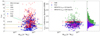 |
Fig. 1. Left panel: concentration-mass relation of the clusters at z = 0.22. The blue and red data points represent the concentration values computed using the P12 and S08 relations, respectively. The various lines display different concentration-mass relation models computed at z = 0.22. Right panel: ratio of the measured concentration, using different methods compared with respect to the Springel et al. (2008b) formalism. The green crosses and magenta pluses display the case in which we compute the concentration by fitting the differential logarithmic density profile outside 10 and 100 h−1 kpc, respectively. |
In Fig. 2, we show the spherically averaged density profiles of two clusters: halo 3 (on the left) and halo 4 (on the right). In each panel, we exhibit the total density profile of the full hydrodinamical simulations and the corresponding dark matter-only runs. The profiles extend up to R200, which is defined as the radius enclosing 200 times the critical density. The solid blue and dashed cyan curves display the NFW profiles using the concentration values as derived from the P12 and S08 relations, respectively. With the solid green and dashed magenta lines, we display the NFW profiles, whose concentration was derived by modelling the logarithmic density profile outside 10 and 100 h−1 kpc, respectively. The figure shows that while for halo-3, the solid blue and green lines describe the total mass density profile of the cluster relatively well, only the green line represents the matter density distribution well for halo 4. This could be due to the fact that while halo-3 has an inner slope dlog ρ/dlog r that is close to −1, the cluster halo-4 has a steeper slope toward the centre. Moreover, the density in the outskirts of the clusters is higher than expected from the NFW profile due to the presence of substructures. These differences are reduced for the projected quantities, highlighting that the NFW prescription is sufficient for the analysis in this paper.
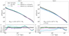 |
Fig. 2. Spherically averaged density profiles of halo 3 and halo 4. In each panel, the solid black curve displays the total matter density profile of the full hydrodynamical runs as considered in this work. For comparison, the dashed grey curve shows the profile of the dark matter-only runs. With solid blue and dashed cyan lines, we show the NFW profiles assuming concentrations as computed using the P12 and S08 formalisms, respectively. With solid green and dashed magenta lines, we show the NFW profiles with concentrations computed by fitting the logarithm profile outside 10 and 100 h−1 kpc, respectively. The profiles extend up to the halo virial radius R200, as computed by AHF. |
We would also like to underline that the extrapolation of these 3D uncertainties into projected quantities is not straightforward and may require adopting some reference concentration-mass relation model (Hoekstra et al. 2013; Simet et al. 2017a,b; Kiiveri et al. 2021; Sommer et al. 2022). We describe how they impact the recovered weak-lensing mass bias in the next section.
3. Cluster weak-lensing simulations
In order to build up the mass maps, we proceeded as follows. From the AHF catalogues, we read the positions of the halo centres in comoving units (xc, yc, zc) and then the particle positions with associated masses and types from the corresponding snapshot file. Each snapshot contains dark matter, gas, and stellar and black hole particles. For each cluster, we considered three random lines of sight corresponding to the axes of the simulation box, along which we projected the cluster particles on a perpendicular plane centred on the cluster centre. We considered particles in a slice of depth ±5 Mpc (3.4 h−1 Mpc) in front of and behind the cluster. The maps had a final size of 5 Mpc on a side, resolved with 20482 pixels, and were produced using Py-SPHViewer (for more details we refer to Benitez-Llambay 2015). The choice of the size of the field of view was motivated by the fact that we are mainly interested in modelling the projected matter density distribution of the main cluster without being much affected by the additional source of uncertainty associated with the large-scale matter density distribution along the line of sight (Hoekstra 2001, 2003). This value also represents a reasonable compromise to avoid influence from low-resolution particles in the re-simulated box. In addition, it is worth stressing that the scatter in the weak-lensing mass bias could be underestimated with respect to what was measured by Becker & Kravtsov (2011), who used a larger line-of-sight integration.
The convergence κ was obtained from the mass map by dividing the mass per pixel by its associated area to obtain the surface density Σ(θ) and by the critical surface density Σcrit (Bartelmann & Schneider 2001), which can be read as
 (6)
(6)
where Dl, Ds, and Dls are the observer-lens, observer-source, and source-lens angular diameter distances, respectively; c represents the speed of light, and G is the universal gravitational constant. The critical surface density is a function of the redshift of the lens and of the source. Our reference weak-lensing maps were created assuming a fixed source redshift of zs = 3.
In Fig. 3, we show three convergence maps of the same cluster, namely halo-4 at z = 0.22. The left, central, and right panels display the system projected along the z-, y-, and x-axis of the comoving re-simulated box, respectively. Because there is no particular selection with respect to the triaxial properties of the cluster haloes, these projections can be seen as random projections, and we therefore refer to them as proj0, proj1, and proj2 in the following.
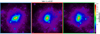 |
Fig. 3. Convergence maps of the three considered random projections of a cluster, namely halo 4 at z = 0.22. The left, central, and right panels show the projections along the z-, y-, and x-axis coordinates of the re-simulated box. The source redshift of the map is fixed at zs = 3. The size of the field of view is 5 Mpc (3.4 h−1 Mpc) on a side and 10 Mpc along the line of sight. The map resolution is 2048 pixels on a side. |
For each cluster, redshift, and projection, we generated weak-lensing convergence maps. Specifically, we considered nine redshifts from z = 0.12 to z = 0.98 as listed in Table 1.
Simulation snapshots (first column) and corresponding redshifts (second column).
From the convergence κ, we define the lensing potential ψ, using the 2D Poisson equation,
 (7)
(7)
which we numerically solved in Fourier space using the fast Fourier transform (FFT) method. Because the FFT algorithm assumes periodic conditions on the boundaries of the map, we zero-padded the exterior of the convergence map by 0.5 Mpc before we computed the discrete Fourier transform, and we then removed the region from the final result.
From the lensing potential ψ, we can then define the two components (γ1, γ2) of the pseudo-vector shear,
 (8)
(8)
 (9)
(9)
where x and y represent the two components of the vector θ.
For each cluster, we used the shear maps to simulate an observed differential surface mass density profile by randomly sampling the field of view with a given number density of expected background sources.
In our analysis, we adopted a background density of sources for weak lensing following the predicted distribution for the ESA Euclid wide-field survey normalised to the total value of 30 galaxies per square arcminute (Laureijs et al. 2011). In the third column of Table 1, we report the average number of background sources beyond each considered cluster redshift, whose corresponding snapshot number is displayed in the first column.
The approach of randomly sampling the shear field has been chosen to mimic the expected average profile of a cluster from a Euclid wide-field exposure. Given the high number density of background sources, the profile has a much smaller scatter than what we consider the complete shear field. We tested this for the halo-4 at z = 0.22 and z = 0.94, generating 10 000 random shear field realisations, finding results consistent with our reference case well within 1σ of the credibility regions of the posteriors.
From the two components of the shear, we defined the tangential shear γt (Umetsu 2020) at each sampled point θi of the map,
 (10)
(10)
where (0, 0) is the centre of the cluster by construction,  and ϕi = arctan(yi/xi). This gives us the possibility to write the excess surface mass density by azimuthally averaging the measured quantities,
 (11)
(11)
where Σ(θ) represents the mass surface density of the lens at a distance θ from the putative cluster centre, and  is its mean within θ.
The approach that we followed in this work aims to quantify the weak-lensing mass bias associated with projection effects and its redshift evolution, depending on the available number density of galaxies from which we can measure the lensing signal induced by the interposed cluster projected mass density distribution. In this way, we quantify the most optimistic weak-lensing mass bias that we expect from Euclid data. In this analysis, we do not assume any uncertainty on the cluster centre, the lens, and source redshifts, which are all assumed to be known with infinite accuracy. Forthcoming analyses within the Euclid Collaboration will be dedicated to studying these systematics and the corresponding propagation into the weak-lensing mass biases and concentration that should be degenerate and more affected by the miscentring (Giocoli et al. 2021; Lesci et al. 2022).
To simulate the weak-lensing signal of each cluster, we built the average excess surface mass density by binning the measured ΔΣ(ri), where ri ≡ Dl θi, in 22 logarithmically equispaced intervals from 0.02 to 1.7 h−1 Mpc from the cluster centre. As an example, in the top panel of Fig. 4, blue, red, and green data points display the simulated ΔΣ profile for three random projections of the cluster halo-4 at z = 0.22, as shown in Fig. 3. In order to limit the analysis to well-constrained shear estimates (depending on the angular binning and on the source density), we considered only radial bins with at least ten simulated data measures. This guaranteed a reliable estimate of the average signal and conservatively neglected bins that are close to the centre, where baryonic effects tend to steepen the profile. However, we tested that considering radial bins with at least one galaxy did not alter the mass bias results of our work. The colours correspond to those used for the panel frame of Fig. 3. The corresponding error bars were computed as
 (12)
(12)
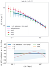 |
Fig. 4. Top panel: excess surface mass density profiles of the three random projections for a cluster-size halo at zl = 0.22, as displayed in Fig. 3. The blue, red, and green data points show the circular averaged profiles of the halo projected along the z-, y-, and x-axis of the re-simulation box. The error bars on the data points account for both the dispersion of the intrinsic ellipticity of background galaxies and the error associated with the average measure in the considered radial bin. The solid blue line displays the best-fit model to proj0, and the shaded region represents the model with a confidence of 68%. Bottom panel: relative difference of the best-fit models assuming different values of the truncation radius Rt with respect to the reference case with t = 3. |
where σe = 0.3 (Hoekstra et al. 2004, 2011; Kilbinger 2015; Euclid Collaboration 2020) is the dispersion of the shape of background source galaxies, and θ1 and θ2 are the lower and the upper bounds of the considered radial annulus. In our error budget, we also included the error of the mean estimated excess surface mass density in each radial interval,  – with σrms, representing the ΔΣ root-mean-square,
 (13)
(13)
⟨ΔΣ⟩ring is the average value, and ng, ring is the number of galaxies in each ring, in order to account for the projected cluster triaxiality, correlated large-scale structures, and the subhalo contribution in each annulus (Gruen et al. 2015, 2011; Umetsu et al. 2020). It is also worth mentioning that this term is negligible with respect to the term that accounts for the intrinsic shape noise. The figure shows that while proj0 and proj2 are similar, proj1 shows a steepening toward the centre. This highlights that depending on the projection, the structural properties recovered from the weak-lensing mass and concentration can be different from each other and can even contrast the three-dimensional properties. In the figure, we highlight that the data binning of the three projections has a different minimum scale because we excluded the rings with fewer than ten galaxies.
4. Analytical models and results
In order to recover the weak-lensing mass and concentration, we modelled the data of the excess surface mass density profile using projected analytical relations. We used the strategy that is being developed within the Euclid Consortium in the implementation of the dedicated processing function: the total density profile is constructed considering the signal coming from the central part of the cluster, called the one-halo term, and the profile caused by correlated large-scale structures is called the two-halo term. Methods based on a non-parametric formalism (Clowe et al. 2004; Bradač et al. 2005, 2006; Diego et al. 2007; Merten et al. 2009; Jauzac et al. 2012; Jullo et al. 2014; Niemiec et al. 2020) may give more accurate and precise mass reconstructions, but at the price of being slow and at high memory cost, and in this way, the methods are hardly applicable to the very large statistics of clusters expected from the Euclid photometric data (Sartoris et al. 2016; Euclid Collaboration 2019).
For the cluster main halo, we adopted a smoothly truncated NFW density profile (BMO; Baltz et al. 2009), defined as
 (14)
(14)
with Rt = t R200, where t is defined as the truncation factor. For our reference model, following the results of Oguri & Hamana (2011), Bellagamba et al. (2019), and Giocoli et al. (2021) we adopted a truncation radius Rt = 3R200. The total mass enclosed within R200, that is, M200, can be thought of as the normalisation of the model and as a mass proxy of the true enclosed mass of the dark matter halo hosting the cluster (Giocoli et al. 2012a). Writing  as the sum in quadrature between the sky-projected coordinate Ddθ and the line-of-sight ζ coordinate, and integrating along ζ, we can write
 (15)
(15)
This projected parametrisation describes the smooth blending of the halo boundary into the connected large-scale structures, regulated by the truncation radius. However, at larger distances from the cluster centre, the projected lensing signal starts to increase due to the large-scale structures of the correlated and the uncorrelated matter along the line of sight: the two-halo term, describing the asymptotic regime far from the halo centre. This term can be written as a function of the integrated linear matter power spectrum weighted by a Bessel function (Oguri & Takada 2011; Oguri & Hamana 2011; Sereno et al. 2017),
 (16)
(16)
where zl represents the cluster (lens) redshift, J2 is the Bessel function of second type, kℓ = ℓ/[(1 + z)Dl(z)] indicates the wave vector mode,  is the background density, Plin, m refers to the linear matter power spectrum, and bh(M; z) is the halo bias, for which we adopt the Tinker et al. (2010) model.
The total model can be read as follows:
 (17)
(17)
It is worth noticing that the two-halo term contribution at small radii is expected to be negligible, but its contribution becomes important with respect to the one-halo term only at scales ≳3 h−1 Mpc (Giocoli et al. 2021; Ingoglia et al. 2022). In their Fig. 1, Giocoli et al. (2021) showed that for distances between 2 and 3 h−1 Mpc from the halo centre, the profile is also sensitive to the truncation radius definition. Given the size of the field of view of our maps, 3.4 h−1 Mpc on a side, the two-halo term has a weak contribution, and we decided to ignore it in our modelling function.
In the top panel of Fig. 4, the solid blue curve stands for the best-fit model to the data points of proj0, associated the median values of the posteriors of log10(M200) and c200. The shaded region marks the 1σ uncertainties of the recovered mass and concentration parameters propagating in the modelling of the ΔΣ profile, associated with the 16th and 84th percentiles of the posterior distributions. In the bottom panel, we show the relative difference of the best-fit models, for which we adopted various values for the truncation radius with respect to the reference case, where we set Rt = 3R200.
The left panel of Fig. 5 displays the posterior distributions of the recovered mass, log10(M200), and concentration, c200, obtained by modelling the three random projections of halo-4 at zl = 0.22 (top panel of Fig. 4). In blue, red, and green, we show the distribution for the projections proj0, proj1, and proj2, respectively, using only the one-halo term in our modelling function and fixing Rt = 3R200. We defined this as the reference model.
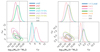 |
Fig. 5. Left panel: posterior distributions of the recovered logarithm of the mass Mwl and concentration cwl obtained by fitting the excess surface mass density profile of the three random projections of halo-4 at z = 0.22. Right panel: posterior distributions obtained by modelling the excess surface mass density profile of halo-4 when it is oriented along proj0, assuming different truncation radii. The blue data display the reference case with a truncation radius Rt = 3R200, and the red, pink, green, and orange data exhibit the results for Rt = t R200 with t = 1, 2, 6, and 9, respectively. The dark and light shaded areas enclose the 1 and 3σ credibility regions, respectively. In both panels, the vertical dashed line marks the true mass of the system, and the horizontal dotted and dashed lines indicate the concentrations computed using the Springel et al. (2008a) and Prada et al. (2012) formalisms, respectively. |
We performed a Monte Carlo Markov chain run assuming a Gaussian log-likelihood between the model and the data as defined within our reference CBL libraries4 (Marulli et al. 2016) that can be read as
 (18)
(18)
where
 (19)
(19)
summing on the number of radial bins. We did not account for reduced shear corrections in the simulations and model, However, observationally this model absorbs the reduced shear impact in the resulting mass bias. We set uniform priors for log10(M200/[h−1 M⊙]) ∈ [12.5, 16] and c200 ∈ [1, 15], and let each MCMC chain run for 16 000 steps. In cyan, purple, and gold, we show the posterior distributions obtained by also adding the contribution of the two-halo term in the modelling function, as expressed by Eq. (16). Comparing the two, we note that the results fully agree with the analysis that does not include the two-halo term, also for high-redshift clusters. This guarantees that for each cluster and redshift, the data that we built by projecting the mass density distribution from the simulations takes a negligible contribution from correlated structures along the line of sight due to the limited size of the field of view (3.4 h−1 Mpc), as discussed earlier.
In the right panel of Fig. 5, we examine the dependence of different assumptions for the truncation radius on the recovered weak-lensing halo mass and concentration, as parametrised in Eq. (14) and inserted into Eq. (15). We show the posterior distributions when t is assumed to be equal to 1 (red), 2 (pink), 3 (blue), 6 (green), and 9 (orange). The figure shows that the different choices result in a diverse recovered concentration: smaller truncation radii prefer lower concentration parameters. When t = 1 (relatively unphysical case) and 2, the mass also tends to be underestimated. For guidance, we underline that in both panels, the dotted and dashed lines refer to the true 3D halo mass and concentrations, adopting the Springel et al. (2008a) and Prada et al. (2012) relations, respectively.
In Fig. 6 we show the weak-lensing mass bias as a function of the cluster true mass M200 for systems at zl = 0.22. The grey data points display the ratio of the weak-lensing mass and the true mass, modelling the excess surface mass density profile with our reference model: a one-halo term with a truncation radius parameter t = 3. The error bars indicate the 16th and 84th percentiles of the posterior distributions for each considered cluster projection. The black solid line shows the moving average of the data. Red, pink, green, and orange lines display the moving average when considering the truncation radius equal to 1, 2, 6, and 9 times R200 in our modelling function, respectively (the corresponding data points are not displayed in the figure). The figure shows that the average weak-lensing cluster mass bias depends on the value of the truncation radius adopted in the modelling. In particular, assuming t = 1, we underestimate the mass by approximately ∼30%. Higher t values increase the weak-lensing mass and therefore decrease the mass bias. For our reference case with t = 3, the average mass bias is as low as ∼7% with a standard deviation shown by the grey shaded region (see also Becker & Kravtsov 2011), thus highlighting that triaxiality is the largest source of intrinsic scattering. The right panel shows the distributions for the corresponding cases independently of the halo mass M200, and the top panel shows the average relative uncertainty for the weak-lensing mass estimates as a function of 3D cluster mass. The filled blue circles report the results by Bahé et al. (2012, hereafter B12), who modelled the weak-lensing mass bias using tangential shear profiles up to 2.2 h−1 Mpc from the cluster centre (while we extended our analysis out to 1.7 h−1 Mpc). Their value is higher than ours, and the authors used only the one-halo term, modelled with a pure NFW profile (we adopted a truncated NFW using the BMO relation), without quantifying the two-halo contribution. In their case, this contribution may not be entirely negligible because their field of view is larger. In addition, they used a dispersion parameter of the intrinsic shape of background source galaxies σe = 0.2, while we adopted a higher value σe = 0.3. All these factors may increase the relative uncertainties in the recovered weak-lensing masses.
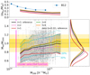 |
Fig. 6. Weak-lensing mass bias as a function of the true cluster mass for all systems at zl = 0.22 for different assumptions of the truncation factor. The data points show the ratio of the recovered weak-lensing mass obtained by fitting the excess surface mass density profile using our reference model with the one-halo term assuming a truncation radius Rt = 3R200 and the true M200 mass. The error bars correspond to the 16th and 84th percentiles of the posterior distribution. The solid black line represents the moving average of the data points. The red, pink, green, and orange lines display the moving average of the data considering the truncation radius parameter equal to t = 1, 2, 6, and 9 in our modelling function, respectively. The dashed and dotted cyan lines indicate 20 and 30% of the scatter, respectively, while the vertical magenta line indicates the minimum cluster mass, which is almost constant with redshift, and which is expected to be detected from the photometric catalogue as predicted by Sartoris et al. (2016). The light and dark yellow bands mark 10% and 20% scatter, respectively. The top subpanel displays the relative weak-lensing mass uncertainty as a function of the true cluster mass. The blue circles show the prediction by B12. The histograms in the right panel show the weak-lensing mass bias distributions over all cluster masses for the various considered cases. |
4.1. Mass bias and concentration
In the spirit of understanding how well we can recover the weak-lensing mass bias when assuming a concentration model, we show in Fig. 7 the posterior distribution of the logarithm of the recovered cluster mass in the case of halo-4 for different concentrations. Generally, they affect the recovered mass. In particular, for a fixed value equal to c200 = 3, no bias on the recovered mass for this specific cluster and projection is detected. More relevant than mass biases for individual realisations are average biases computed for representative cluster samples, which show a similar dependence on the adopted concentration mass relation (e.g Sommer et al. 2022).
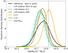 |
Fig. 7. Posterior distributions when the logarithm of the cluster mass is recovered for proj0 of halo-4 at z = 0.22. The black curve shows the reference case, where we model both the mass and the concentration, as in the top panel of Fig. 5. The other histograms show the posteriors when a parametrisation of the concentration-mass relation is assumed; in particular, the orange and olive curves refer to the cases with a constant value of c200 = 3 and c200 = 4, respectively. The vertical dashed black line marks the true value of M200 as computed by AHF. |
The average weak-lensing mass bias as a function of the true cluster mass is displayed in Fig. 8. The black line shows our reference case. The solid green, dashed cyan, and dark red lines correspond to the moving average when assuming different concentration-mass relation models: Zhao et al. (2009), Meneghetti et al. (2014), and Sereno et al. (2017), respectively. The orange and olive curves display the results assuming a fixed value c200 = 3 and c200 = 4, respectively. With reference to the P12 (S08) model, the average concentration of clusters at z = 0.22 is ⟨c200⟩ = 4 (5) (see the left panel of Fig. 1). The corresponding dotted coloured lines display the linear regressions,
 (20)
(20)
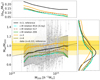 |
Fig. 8. Weak-lensing mass biases for clusters at z = 0.22. The points are the same as in Fig. 6. The different line styles and coloured curves display the moving averages for different approaches when modelling the concentration. The solid black line refers to the reference case, where we varied both the mass and the concentration in our MCMC analysis. The solid green, dotted cyan, and dark red curves refer to the case in which we assumed a concentration-mass relation model, as in the figure label. On the other side, the orange and olive curves assume a constant value of c200 = 3 and c200 = 4, respectively. The dotted coloured lines display the linear regressions to the moving average and the corresponding uncertainty (not shown for the orange data for clarity). The top and left panels show the mean relative mass uncertainties as a function of the true cluster mass and the distributions of the weak-lensing mass biases, respectively. |
where M14.5 = 1014.5 h−1 M⊙ for the reference and c200 = 3 cases (see Table 3). The average values were computed assuming a step size = 0.1 and a bin size = 0.3 in log(M200).
The top subpanel shows that the average relative scatter as a function of M200 is reduced by approximately a factor of two when a deterministic model for the concentration is assumed with respect to the case in which we varied it inside the Monte Carlo analyses. The right panel displays the distribution of the relative mass ratio.
4.2. Mass bias and relaxation criteria
The morphological properties of galaxy clusters depend on their mass-assembly history. Typically, clusters that experienced recent merging events may contain a larger fraction of their mass in substructures and eventually a mass centroid that is not coincident with the position of the density peak due to the presence of multi-mass components. These properties manifest themselves in a variety of observables at different wavelengths from X-ray to the radio band. The projected mass recovered using weak-lensing data is also influenced by the level of dynamical relaxation of the lens. In this section, we quantify these dependences.
In the left panel of Fig. 9, we display the scatter plot of clusters at z = 0.22 for parameters fsub and xoff, which we used to define the relaxation status of a system; see their definition in Sect. 2. We defined as relaxed systems those with fsub < 0.1 and xoff < 0.05R200, that is, the clusters lying in the lower left white rectangle of the figure: 147 over 324 objects satisfy this condition. Our relaxed clusters are circled in green, while unrelaxed systems are displayed with magenta circles. In the figure, we also mark the relaxation criterion adopted by Cui et al. (2018): xoff < 0.04R200 (with a dotted vertical line) and with a virial ratio 0.85 < η < 1.15. The latter condition is portrayed in the figure by colouring the data points in blue or otherwise in yellow. The relation criterion adopted by Cui et al. (2018) is satisfied by 91 systems. In the right panel, we display the weak-lensing mass bias as a function of the cluster mass for the relaxed (green) and the unrelaxed (magenta) clusters. The solid green and magenta curves represent the moving average of the two samples. The corresponding dashed curves refer to the cases in which the relaxation criterion by Cui et al. (2018) was adopted, who also used information on the virial energy ratio. The top subpanel shows that the average relative uncertainty in the recovered mass is lower for relaxed systems, even when the differences between the two cases are small to some extent, and the relative mass bias has a lower scatter than for unrelaxed clusters (right subpanel). This highlights the fact that unrelaxed systems cannot be modelled well by the single-halo model (Lee et al. 2023). As in previous figures, and to highlight the differences between the relaxed and unrelaxed samples, the dotted coloured lines display the linear regressions to the moving average and the corresponding uncertainty. The best-fit parameters and the corresponding uncertainties, as expressed in Eq. (20) for the relaxed and unrelaxed sample at z = 0.22 are shown in Table 2, which can be compared with the full sample in Table 3.
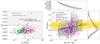 |
Fig. 9. Left panel: relaxation criteria for the clusters at z = 0.22. In our analysis, we assumed the systems to be relaxed when their mass fraction in substructures fsub < 0.1 and their centre of mass offset xoff < 0.05R200, indicated by the rectangular white region in the bottom left corner. Our relaxed (unrelaxed) clusters are circled in green (purple). For comparison, we also mark the relaxation criterion by Cui et al. (2018): fsub < 0.1, xoff < 0.04R200 and the energy parameter 0.85 < η < 1.15 (filled blue circle, otherwise gold). Right panel: weak-lensing mass bias as a function of the true mass of the cluster. The circled green and magenta data points correspond to systems that are or are not relaxed, respectively. The solid green and magenta data points show the moving average of the two samples. For comparison, the dashed lines, coloured accordingly, show the results using the relaxation criteria by Cui et al. (2018). The sub-panel on the right displays the mass bias distributions for the various cluster samples, and the top panel is the average relative scatter in the weak-lensing mass estimates as a function of M200. |
4.3. Mass bias along preferential directions
The reliability with which the cluster mass can be recovered is also related to the orientation of the ellipsoid that describes the moment of inertia tensor with respect to the line of sight (Sereno & Zitrin 2012; Sereno et al. 2013, 2018; Despali et al. 2014, 2017). Herbonnet et al. (2022) have shown that the shape of the bright central galaxy can give unbiased information about the shape of the total halo mass ellipsoid and that the recovered mass via weak gravitational lensing is biased low (high) if the halo is oriented along the minor (major) axis with respect to the observer. In this section, we quantify in detail how the mass bias depends on the orientation of the mass tensor ellipsoid with respect to the line of sight. Following Sereno et al. (2017) and Umetsu et al. (2020), we define the weak-lensing signal-to-noise ratio as
 (21)
(21)
where the variable i runs on all the considered radial bins.
In the left panel of Fig. 10, we show the weak-lensing signal-to-noise ratio of clusters at z = 0.22. The grey histogram shows the distribution of the S/N for all considered random projections, while the black curve displays the kernel density estimate (KDE) of the binned histogram. The blue (dashed), red (dotted), and green (dot-dashed) curves refer to the distributions of the weak-lensing signal-to-noise ratios when the cluster ellipsoids are oriented with respect to the minor, intermediate, and major axis of the mass tensor ellipsoid. The triaxial parameters are those computed by the AHF algorithm (we refer to Knollmann & Knebe 2009 and Cui et al. 2018 for more details). The results confirm that orientation matters: The weak-lensing signal-to-noise ratio distributions are shifted toward higher (lower) values when clusters are oriented along the major (minor) axis of the mass tensor ellipsoid with the line of sight. Projection effects also impact the weak-lensing mass bias and the scatter, as we can observe in the right panel of Fig. 10. The mass bias when clusters are preferentially selected either along the line of sight or in the plane of the sky is approximately +25% or −25%. The top subpanel also shows that the average relative weak-lensing mass uncertainty varies with the orientation of the cluster ellipsoid.
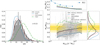 |
Fig. 10. Left panel: weak-lensing signal-to-noise ratio distributions for the sample of clusters at z = 0.22. The shaded grey histogram shows the distribution for the clusters oriented along random projections, namely the x, y, and z Cartesian axes of the re-stimulated box region. The solid black curve represents the KDE of the grey discrete histogram. The blue (dashed), red (dotted), and green (dot-dashed) curves refer to the KDE of the distributions when systems are oriented along the minor, intermediate, and major axis of the cluster ellipsoid, respectively. Right panel: weak-lensing derived mass bias as a function of the true mass of the cluster. The solid blue (dashed), red (dotted), and green (dot-dashed) lines display the moving average of the corresponding mass bias data points of the preferential projections, minor, intermediate, and major axis, respectively. The top and right sub-panels display the relative mass uncertainties as a function of the true mass and the weak-lensing mass bias distributions, respectively. |
Before we conclude this section, we briefly comment on cluster detections and orientation biases. At fixed mass, when systems are oriented along the major axis of the ellipsoid, they tend to have a more compact and concentrated galaxy satellite distribution on average than when they are oriented along the minor axis: this indicates that optical cluster finder algorithms in observational data may be affected by orientation bias (Wu et al. 2022). We plan to examine and analyse this argument in more detail in a future dedicated work.
For example, in Fig. 11, the solid magenta curve shows the average excess surface mass density profile of the six projections of cluster halo-4 at redshift z = 0.22. The solid red, blue, and green lines are the individual profiles for three random projections. The dotted blue, orange, and green curves show the profiles when the cluster is oriented along the minor, intermediate, and major axis of the ellipsoid with respect to the line of sight, as done previously. Only radial bins with more than ten galaxies are shown.
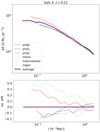 |
Fig. 11. Top panel: average excess surface mass density profile averaging six different projections of the same cluster (halo-4 at z = 0.22): three randoms and three preferentials. For comparison, the solid blue, red, and green curves show the individual profiles around the three random projections, and the dashed blue, orange, and green lines show the cluster oriented along the minor, intermediate, and major axis of the moment of inertia tensor ellipsoid. Bottom panel: relative difference of the individual profiles with respect to the averaged one. |
4.4. Reshift evolution of the mass bias
The expected source redshift distribution available for weak-lensing measurements tells us how many background sources can be used to probe the total projected mass distribution of a cluster acting as a gravitational lens. The reliability of the lensing measurement also depends on the intrinsic magnitude of the sources and their projected distance with respect to the cluster centre because of possible confusion with cluster member galaxies. The weak-lensing signal-to-noise ratio of individual clusters is also modulated by the expected available number density of sources expected from the Euclid wide survey, as we display in Fig. 12. Low-redshift systems have a higher weak-lensing signal-to-noise ratio than high-redshift systems. In the figure, we consider only the measurement of the three random projections per cluster because we have already discussed in the previous section that the three preferential projections need particular attention. We also underline that possible stacking procedures will shift the expected weak-lensing signal-to-noise ratio distributions toward higher values by a factor that is approximately equal to the square root of the number of systems that are combined.
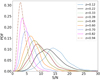 |
Fig. 12. Individual cluster weak-lensing signal-to-noise ratio distributions for random projections and different redshifts as expected in the Euclid wide-field survey of a cluster population that is representative of the simulated clusters studied here. |
In Fig. 13 we show the average weak-lensing mass bias for the different redshifts, considering the three random projections per cluster, and cluster masses with M200 > 1014 M⊙. In our modelling analysis, we assumed a uniform range both for the logarithm of the mass and for the concentration parameter. Higher-redshift clusters tend to be more biased low on average than M200, as a result of their lower signal-to-noise ratio. The top subpanel shows that the relative error of the recovered weak-lensing mass tends to be larger for systems at higher redshifts, which is due to the lower background source densities and average lensing efficiencies for these systems. In Table 3 we summarise the values of the parameters describing the linear fitting functions and the corresponding uncertainties, as in Eq. (20), at different redshifts, for the reference modelling case, and assuming a constant concentration c200 = 3.
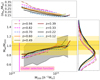 |
Fig. 13. Average weak-lensing mass bias as a function of the cluster halo mass M200 for different lens redshifts. We consider all clusters with M200 > 1014 M⊙, which is above the minimum mass expected to be selected in the photometric catalogue (Sartoris et al. 2016), and which are relatively constant with redshift. The right and top subpanels are the same as in Fig. 6. |
Averaging over all cluster masses with M200 > 1014 M⊙, we display in Fig. 14 the weak-lensing mass bias as a function of the lens redshift. The black circles show the results averaged over all random projections. Higher-redshift systems are more biased low than low redshift ones. The blue crosses and green squares represent the redshift evolution of the mass bias when the clusters are oriented along the minor or major axis of the ellipsoid with respect to the line of sight, respectively. The orange diamonds and olive pentagons refer to the case when in individual random projections we modelled only the logarithm of the cluster mass while keeping the concentration fixed to c200 = 3 and c200 = 4, respectively. These values represent the typical concentration parameters of the cluster size-halo as highlighted in different numerical simulation analyses (Zhao et al. 2009; Giocoli et al. 2012b; Ludlow et al. 2012, 2016). Assuming a fixed concentration c200 = 3 in our modelling analysis of the weak-lensing signal of individual clusters, we can recover a weak-lensing mass that is biased by no more than 5% on average with respect to the true one up to redshift z = 0.7 – positive for z < 0.4 and negative at higher redshift. The error bars associated with all data points correspond to the errors on the mean value. The dotted lines, which differ more significantly from each other at z > 0.6, display the results for the whole cluster sample with no minimum mass cut.
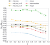 |
Fig. 14. Average cluster weak-lensing mass bias as a function of the lens redshift for clusters with M200 > 1014 M⊙. The various data points and colours refer to different ways of computing the cluster masses. The black circles display the case of random projections and modelling both the halo mass and concentration. The orange diamonds, and olive pentagons show the cases in which we assumed a fixed concentration parameter (three and four, respectively)and we fit only the halo mass. The light blue crosses, red triangles, and green squares show the average mass bias for the three particular projections along the minor, the intermediate, and the major axis, respectively. The dotted lines, which slightly deviated from the data points only at z > 0.6, correspond to the results for the whole cluster sample, with no minimum mass cut. |
The impact of the scatter and the redshift evolution of the cluster mass bias will be highly important for cluster cosmology. Different future works have already been planned and organised to further assess systematics and nuisance parameters in the cosmological likelihood pipeline.
5. Summary and conclusions
We performed a systematic study of the weak-lensing mass bias using hydrodynamical simulations of clusters. We simulated the expected excess surface mass density profile from the expected number density of background sources of the ESA Euclid wide-field survey, normalised to 30 galaxies per square arcminute. We adopted a projected truncated NFW profile to model the data. Our main results are summarised as follows:
-
Individual weak-lensing masses Mwl are typically lower by 5% on average than the true one. Various projections of the same cluster may have different recovered weak-lensing masses that differ by up to 30%: Cluster triaxiality represents the largest source of intrinsic scattering.
-
In our reference model, we adopted a truncation radius of three times R200. A lower truncation radius returns a more biased weak-lensing mass: From t = 1 to t = 9, the mass bias for clusters at z = 0.22 ranges from −30% to a few percent.
-
When we modelled the data set, we also investigated the impact of using a concentration both dependent, in one case, and independent of the total mass in another case. We find that this systematically impacts the recovered weak-lensing mass (see e.g. also Sommer et al. 2022).
-
Relaxed clusters, being better described by a one-halo projected density profile, are less biased than the unrelaxed clusters by approximately 3%.
-
The weak-lensing mass of clusters that are oriented along the major (minor) axis of the mass tensor ellipsoid is overestimated (underestimated) by approximately +(−) 25%.
-
Averaging over all masses, when the concentration is varied as well, the negative mass bias tends to increase as a function of redshift. However, when a fixed concentration is assumed, this effect is reduced. The increase in negative mass bias with redshift is due to the lower S/N of the weak-lensing mass constraints of high-redshift clusters. As demonstrated by Sommer et al. (2022), this S/N dependence can be avoided when the weak-lensing mass scatter is separated into an intrinsic component (e.g. due to variations in density profiles and substructures) and a shape noise component (e.g. Bocquet et al. 2019; Chiu et al. 2022).
The use of galaxy clusters as cosmological probes relies on the accuracy and precision of mass measurements. The future ESA Euclid mission will make use of weak gravitational lensing to determine the projected total mass. We have quantified the accuracy and bias effects by using dedicated lensing simulations of clusters in a variety of dynamical states and at different redshifts, based on a specific set of hydrodynamical simulations: the Three Hundred clusters. While the mass bias depends on the considered choice of the modelling function, the scatter is driven by the complex triaxial structure of galaxy clusters. However, assuming a fixed value c200 = 3 for the concentration parameter when modelling the data of individual clusters produces less unbiased results, at least for the set of simulated clusters we analysed in this work.
We would like to conclude by underling that future works will be devoted to study whether these calibrations are robust against variations in the astrophysical processes included in the simulations. This paves the way for future cluster analyses and opens new perspectives for the cosmological exploitation of galaxy clusters.
The mass within the radius that encloses 200 times the critical density of the universe at a given redshift.
Defined as the total number of member galaxies within the cluster radius R200, above a typical characteristic luminosity.
Acknowledgments
C.G., M.M., and L.M. acknowledge support from the grant PRIN-MIUR 2017 WSCC32 ZOOMING, and the support from the grant ASI n.2018-23-HH.0. C.G. acknowledges funding from the Italian National Institute of Astrophysics under the grant “Bando PrIN 2019”, PI: Viola Allevato and from the HPC-Europa3 Transnational Access programme HPC17VDILO. G.C. also thanks the support from INAF theory Grant 2022: Illuminating Dark Matter using weak-lensing by Cluster Satellites, PI: Carlo Giocoli. M.M. acknowledges financial support from PRIN-MIUR grant and 2020SKSTHZ, INAF “main-stream” 1.05.01.86.20: “Deep and wide view of galaxy clusters (P.I.: M. Nonino)” and INAF “main-stream” 1.05.01.86.31 “The deepest view of high-redshift galaxies and globular cluster precursors in the early Universe” (P.I.: E. Vanzella). S.B. and M.M. acknowledge financial support from the InDark INFN Grant. G.Y. and A.K. would like to thank the Ministerio de Ciencia e Innovación (Spain) for financial support under research grant PID2021-122603NB-C21. The THREE HUNDRED simulations used in this work have been performed in the MareNostrum Supercomputer at the Barcelona Supercomputing Center, thanks to CPU time granted by the Red Española de Supercomputación. W.C. is supported by the STFC AGP Grant ST/V000594/1 and the Atracción de Talento Contract no. 2020-T1/TIC-19882 granted by the Comunidad de Madrid in Spain. He also thanks the Ministerio de Ciencia e Innovación (Spain) for financial support under Project grant PID2021-122603NB-C21. He further acknowledges the science research grants from the China Manned Space Project with NO. CMS-CSST-2021-A01 and CMS-CSST-2021-B01. We acknowledge the use of computational resources from the parallel computing cluster of the Open Physics Hub (https://site.unibo.it/openphysicshub/en) at the Physics and Astronomy Department in Bologna. T.S. acknowledges support from FFG grant number 899537. C.J.M. acknowledges FCT and POCH/FSE (EC) support through Investigador FCT Contract 2021.01214.CEECIND/CP1658/CT0001. The figures with the corner plots displaying the posterior distributions have been produced using the package pygtc developed by Bocquet & Carter (2016). The authors acknowledge the Euclid Consortium, the European Space Agency, and a number of agencies and institutes that have supported the development of Euclid, in particular the Academy of Finland, the Agenzia Spaziale Italiana, the Belgian Science Policy, the Canadian Euclid Consortium, the French Centre National d’Etudes Spatiales, the Deutsches Zentrum für Luft- und Raumfahrt, the Danish Space Research Institute, the Fundação para a Ciência e a Tecnologia, the Ministerio de Ciencia e Innovación, the National Aeronautics and Space Administration, the National Astronomical Observatory of Japan, the Netherlandse Onderzoekschool Voor Astronomie, the Norwegian Space Agency, the Romanian Space Agency, the State Secretariat for Education, Research and Innovation (SERI) at the Swiss Space Office (SSO), and the United Kingdom Space Agency. A complete and detailed list is available on the Euclid web site (http://www.euclid-ec.org).
References
- Ahad, S. L., Bahé, Y. M., Hoekstra, H., van der Burg, R. F. J., & Muzzin, A. 2021, MNRAS, 504, 1999 [CrossRef] [Google Scholar]
- Allen, S. W., Evrard, A. E., & Mantz, A. B. 2011, ARA&A, 49, 409 [Google Scholar]
- Angelinelli, M., Vazza, F., Giocoli, C., et al. 2020, MNRAS, 495, 864 [NASA ADS] [CrossRef] [Google Scholar]
- Ansarifard, S., Rasia, E., Biffi, V., et al. 2020, A&A, 634, A113 [NASA ADS] [CrossRef] [EDP Sciences] [Google Scholar]
- Applegate, D. E., Mantz, A., Allen, S. W., et al. 2016, MNRAS, 457, 1522 [NASA ADS] [CrossRef] [Google Scholar]
- Bahé, Y. M., McCarthy, I. G., & King, L. J. 2012, MNRAS, 421, 1073 [NASA ADS] [CrossRef] [Google Scholar]
- Baltz, E. A., Marshall, P., & Oguri, M. 2009, JCAP, 2009, 015 [Google Scholar]
- Barnes, D. J., Vogelsberger, M., Pearce, F. A., et al. 2021, MNRAS, 506, 2533 [NASA ADS] [CrossRef] [Google Scholar]
- Bartelmann, M. 2010, CQG, 27, 233001 [NASA ADS] [CrossRef] [Google Scholar]
- Bartelmann, M., & Schneider, P. 2001, Phys. Rep., 340, 291 [Google Scholar]
- Beck, A. M., Dolag, K., & Donnert, J. M. F. 2016, MNRAS, 458, 2080 [NASA ADS] [CrossRef] [Google Scholar]
- Becker, M. R., & Kravtsov, A. V. 2011, ApJ, 740, 25 [NASA ADS] [CrossRef] [Google Scholar]
- Bellagamba, F., Maturi, M., Hamana, T., et al. 2011, MNRAS, 413, 1145 [NASA ADS] [CrossRef] [Google Scholar]
- Bellagamba, F., Roncarelli, M., Maturi, M., & Moscardini, L. 2018, MNRAS, 473, 5221 [NASA ADS] [CrossRef] [Google Scholar]
- Bellagamba, F., Sereno, M., Roncarelli, M., et al. 2019, MNRAS, 484, 1598 [Google Scholar]
- Benitez-Llambay, A. 2015, https://doi.org/10.5281/zenodo.21703 [Google Scholar]
- Biffi, V., Borgani, S., Murante, G., et al. 2016, ApJ, 827, 112 [NASA ADS] [CrossRef] [Google Scholar]
- Biviano, A., Murante, G., Borgani, S., et al. 2006, A&A, 456, 23 [NASA ADS] [CrossRef] [EDP Sciences] [Google Scholar]
- Biviano, A., Rosati, P., Balestra, I., et al. 2013, A&A, 558, A1 [Google Scholar]
- Bocquet, S., & Carter, F. W. 2016, J. Open Source Softw., 1 [Google Scholar]
- Bocquet, S., Saro, A., Mohr, J. J., et al. 2015, ApJ, 799, 214 [NASA ADS] [CrossRef] [Google Scholar]
- Bocquet, S., Saro, A., Dolag, K., & Mohr, J. J. 2016, MNRAS, 456, 2361 [Google Scholar]
- Bocquet, S., Dietrich, J. P., Schrabback, T., et al. 2019, ApJ, 878, 55 [Google Scholar]
- Bocquet, S., Heitmann, K., Habib, S., et al. 2020, ApJ, 901, 5 [Google Scholar]
- Bonamigo, M., Despali, G., Limousin, M., et al. 2015, MNRAS, 449, 3171 [NASA ADS] [CrossRef] [Google Scholar]
- Bradač, M., Schneider, P., Lombardi, M., & Erben, T. 2005, A&A, 437, 39 [NASA ADS] [CrossRef] [EDP Sciences] [Google Scholar]
- Bradač, M., Clowe, D., Gonzalez, A. H., et al. 2006, ApJ, 652, 937 [CrossRef] [Google Scholar]
- Capasso, R., Saro, A., Mohr, J. J., et al. 2019, MNRAS, 482, 1043 [NASA ADS] [CrossRef] [Google Scholar]
- Castro, T., Borgani, S., Dolag, K., et al. 2021, MNRAS, 500, 2316 [Google Scholar]
- Chiu, I. N., Ghirardini, V., Liu, A., et al. 2022, A&A, 661, A11 [NASA ADS] [CrossRef] [EDP Sciences] [Google Scholar]
- Chua, K. T. E., Pillepich, A., Rodriguez-Gomez, V., et al. 2017, MNRAS, 472, 4343 [NASA ADS] [CrossRef] [Google Scholar]
- Clowe, D., Gonzalez, A., & Markevitch, M. 2004, ApJ, 604, 596 [NASA ADS] [CrossRef] [Google Scholar]
- Cromer, D., Battaglia, N., Miyatake, H., & Simet, M. 2022, JCAP, 2022, 034 [CrossRef] [Google Scholar]
- Cropper, M., Pottinger, S., Niemi, S., et al. 2016, in Space Telescopes and Instrumentation 2016: Optical, Infrared, and Millimeter Wave, eds. H. A. MacEwen, G. G. Fazio, M. Lystrup, et al., SPIE Conf. Ser., 9904, 99040Q [NASA ADS] [Google Scholar]
- Cui, W., Knebe, A., Yepes, G., et al. 2018, MNRAS, 480, 2898 [Google Scholar]
- Cui, W., Dave, R., Knebe, A., et al. 2022, MNRAS, 514, 977 [NASA ADS] [CrossRef] [Google Scholar]
- Cusworth, S. J., Kay, S. T., Battye, R. A., & Thomas, P. A. 2014, MNRAS, 439, 2485 [NASA ADS] [CrossRef] [Google Scholar]
- Damsted, S., Finoguenov, A., Clerc, N., et al. 2023, A&A, 676, A127 [NASA ADS] [CrossRef] [EDP Sciences] [Google Scholar]
- Debackere, S. N. B., Schaye, J., & Hoekstra, H. 2021, MNRAS, 505, 593 [NASA ADS] [CrossRef] [Google Scholar]
- Debackere, S. N. B., Hoekstra, H., & Schaye, J. 2022a, MNRAS, 515, 6023 [CrossRef] [Google Scholar]
- Debackere, S. N. B., Hoekstra, H., Schaye, J., Heitmann, K., & Habib, S. 2022b, MNRAS, 515, 3383 [NASA ADS] [CrossRef] [Google Scholar]
- De Lucia, G., Kauffmann, G., Springel, V., et al. 2004, MNRAS, 348, 333 [NASA ADS] [CrossRef] [Google Scholar]
- Despali, G., Giocoli, C., & Tormen, G. 2014, MNRAS, 443, 3208 [Google Scholar]
- Despali, G., Giocoli, C., Angulo, R. E., et al. 2016, MNRAS, 456, 2486 [NASA ADS] [CrossRef] [Google Scholar]
- Despali, G., Giocoli, C., Bonamigo, M., Limousin, M., & Tormen, G. 2017, MNRAS, 466, 181 [Google Scholar]
- Diego, J. M., Tegmark, M., Protopapas, P., & Sandvik, H. B. 2007, MNRAS, 375, 958 [NASA ADS] [CrossRef] [Google Scholar]
- Dietrich, J. P., Bocquet, S., Schrabback, T., et al. 2019, MNRAS, 483, 2871 [Google Scholar]
- Ettori, S., & Eckert, D. 2022, A&A, 657, L1 [NASA ADS] [CrossRef] [EDP Sciences] [Google Scholar]
- Euclid Collaboration (Adam, R., et al.) 2019, A&A, 627, A23 [NASA ADS] [CrossRef] [EDP Sciences] [Google Scholar]
- Euclid Collaboration (Blanchard, A., et al.) 2020, A&A, 642, A191 [NASA ADS] [CrossRef] [EDP Sciences] [Google Scholar]
- Euclid Collaboration (Scaramella, R., et al.) 2022, A&A, 662, A112 [NASA ADS] [CrossRef] [EDP Sciences] [Google Scholar]
- Euclid Collaboration (Castro, T., et al.) 2023, A&A, 671, A100 [CrossRef] [EDP Sciences] [Google Scholar]
- Gao, L., White, S. D. M., Jenkins, A., Stoehr, F., & Springel, V. 2004, MNRAS, 355, 819 [Google Scholar]
- Gianfagna, G., De Petris, M., Yepes, G., et al. 2021, MNRAS, 502, 5115 [NASA ADS] [CrossRef] [Google Scholar]
- Giocoli, C., Tormen, G., & van den Bosch, F. C. 2008, MNRAS, 386, 2135 [NASA ADS] [CrossRef] [Google Scholar]
- Giocoli, C., Tormen, G., Sheth, R. K., & van den Bosch, F. C. 2010, MNRAS, 404, 502 [NASA ADS] [Google Scholar]
- Giocoli, C., Tormen, G., & Sheth, R. K. 2012a, MNRAS, 422, 185 [NASA ADS] [CrossRef] [Google Scholar]
- Giocoli, C., Meneghetti, M., Bartelmann, M., Moscardini, L., & Boldrin, M. 2012b, MNRAS, 421, 3343 [Google Scholar]
- Giocoli, C., Meneghetti, M., Ettori, S., & Moscardini, L. 2012c, MNRAS, 426, 1558 [NASA ADS] [CrossRef] [Google Scholar]
- Giocoli, C., Meneghetti, M., Metcalf, R. B., Ettori, S., & Moscardini, L. 2014, MNRAS, 440, 1899 [NASA ADS] [CrossRef] [Google Scholar]
- Giocoli, C., Marulli, F., Moscardini, L., et al. 2021, A&A, 653, A19 [NASA ADS] [CrossRef] [EDP Sciences] [Google Scholar]
- Gonzalez, A. 2014, in Building the Euclid Cluster Survey - Scientific Program, Proceedings of a Conference held July 6-11 2014 at the Sexten Center for Astrophysics, 7 [Google Scholar]
- Grandis, S., Mohr, J. J., Dietrich, J. P., et al. 2019, MNRAS, 488, 2041 [NASA ADS] [Google Scholar]
- Grandis, S., Bocquet, S., Mohr, J. J., Klein, M., & Dolag, K. 2021, MNRAS, 507, 5671 [NASA ADS] [CrossRef] [Google Scholar]
- Gruen, D., Bernstein, G. M., Lam, T. Y., & Seitz, S. 2011, MNRAS, 416, 1392 [CrossRef] [Google Scholar]
- Gruen, D., Seitz, S., Becker, M. R., Friedrich, O., & Mana, A. 2015, MNRAS, 449, 4264 [NASA ADS] [CrossRef] [Google Scholar]
- Henson, M. A., Barnes, D. J., Kay, S. T., McCarthy, I. G., & Schaye, J. 2017, MNRAS, 465, 3361 [NASA ADS] [CrossRef] [Google Scholar]
- Herbonnet, R., Crawford, A., Avestruz, C., et al. 2022, MNRAS, 513, 2178 [NASA ADS] [CrossRef] [Google Scholar]
- Hoekstra, H. 2001, A&A, 370, 743 [NASA ADS] [CrossRef] [EDP Sciences] [Google Scholar]
- Hoekstra, H. 2003, MNRAS, 339, 1155 [NASA ADS] [CrossRef] [Google Scholar]
- Hoekstra, H., Yee, H. K. C., & Gladders, M. D. 2004, ApJ, 606, 67 [Google Scholar]
- Hoekstra, H., Hartlap, J., Hilbert, S., & van Uitert, E. 2011, MNRAS, 412, 2095 [NASA ADS] [CrossRef] [Google Scholar]
- Hoekstra, H., Bartelmann, M., Dahle, H., et al. 2013, Space Sci. Rev., 177, 75 [NASA ADS] [CrossRef] [Google Scholar]
- Ingoglia, L., Covone, G., Sereno, M., et al. 2022, MNRAS, 511, 1484 [NASA ADS] [CrossRef] [Google Scholar]
- Jauzac, M., Jullo, E., Kneib, J.-P., et al. 2012, MNRAS, 426, 3369 [Google Scholar]
- Jullo, E., Pires, S., Jauzac, M., & Kneib, J.-P. 2014, MNRAS, 437, 3969 [NASA ADS] [CrossRef] [Google Scholar]
- Jung, S. L., Rennehan, D., Saeedzadeh, V., et al. 2022, MNRAS, 515, 22 [NASA ADS] [CrossRef] [Google Scholar]
- Kiiveri, K., Gruen, D., Finoguenov, A., et al. 2021, MNRAS, 502, 1494 [NASA ADS] [CrossRef] [Google Scholar]
- Kilbinger, M. 2015, Rep. Prog. Phys., 78, 086901 [Google Scholar]
- Klypin, A., Yepes, G., Gottlöber, S., Prada, F., & Heß, S. 2016, MNRAS, 457, 4340 [Google Scholar]
- Knollmann, S. R., & Knebe, A. 2009, ApJS, 182, 608 [Google Scholar]
- Kravtsov, A. V., & Borgani, S. 2012, ARA&A, 50, 353 [Google Scholar]
- Lau, E. T., Kravtsov, A. V., & Nagai, D. 2009, ApJ, 705, 1129 [NASA ADS] [CrossRef] [Google Scholar]
- Laureijs, R., Amiaux, J., Arduini, S., et al. 2011, ArXiv e-prints [arXiv:1110.3193] [Google Scholar]
- Lee, W., Cha, S., Jee, M. J., et al. 2023, ApJ, 945, 71 [NASA ADS] [CrossRef] [Google Scholar]
- Lesci, G. F., Marulli, F., Moscardini, L., et al. 2022, A&A, 659, A88 [NASA ADS] [CrossRef] [EDP Sciences] [Google Scholar]
- Ludlow, A. D., Navarro, J. F., Li, M., et al. 2012, MNRAS, 427, 1322 [NASA ADS] [CrossRef] [Google Scholar]
- Ludlow, A. D., Bose, S., Angulo, R. E., et al. 2016, MNRAS, 460, 1214 [Google Scholar]
- Martizzi, D., Mohammed, I., Teyssier, R., & Moore, B. 2014, MNRAS, 440, 2290 [NASA ADS] [CrossRef] [Google Scholar]
- Marulli, F., Veropalumbo, A., & Moresco, M. 2016, Astron. Comput., 14, 35 [Google Scholar]
- Maturi, M., Bellagamba, F., Radovich, M., et al. 2019, MNRAS, 485, 498 [Google Scholar]
- Meneghetti, M., & Rasia, E. 2013, ArXiv e-prints [arXiv:1303.6158] [Google Scholar]
- Meneghetti, M., Melchior, P., Grazian, A., et al. 2008, A&A, 482, 403 [NASA ADS] [CrossRef] [EDP Sciences] [Google Scholar]
- Meneghetti, M., Rasia, E., Merten, J., et al. 2010, A&A, 514, A93 [NASA ADS] [CrossRef] [EDP Sciences] [Google Scholar]
- Meneghetti, M., Rasia, E., Vega, J., et al. 2014, ApJ, 797, 34 [Google Scholar]
- Merten, J., Cacciato, M., Meneghetti, M., Mignone, C., & Bartelmann, M. 2009, A&A, 500, 681 [NASA ADS] [CrossRef] [EDP Sciences] [Google Scholar]
- Mostoghiu, R., Knebe, A., Cui, W., et al. 2019, MNRAS, 483, 3390 [NASA ADS] [CrossRef] [Google Scholar]
- Navarro, J. F., Frenk, C. S., & White, S. D. M. 1996, ApJ, 462, 563 [Google Scholar]
- Navarro, J. F., Frenk, C. S., & White, S. D. M. 1997, ApJ, 490, 493 [Google Scholar]
- Niemiec, A., Jauzac, M., Jullo, E., et al. 2020, MNRAS, 493, 3331 [CrossRef] [Google Scholar]
- Oguri, M., & Hamana, T. 2011, MNRAS, 414, 1851 [NASA ADS] [CrossRef] [Google Scholar]
- Oguri, M., & Takada, M. 2011, Phys. Rev. D, 83, 023008 [NASA ADS] [CrossRef] [Google Scholar]
- Ondaro-Mallea, L., Angulo, R. E., Zennaro, M., Contreras, S., & Aricò, G. 2022, MNRAS, 509, 6077 [Google Scholar]
- Planck Collaboration XIII. 2016, A&A, 594, A13 [NASA ADS] [CrossRef] [EDP Sciences] [Google Scholar]
- Planelles, S., Borgani, S., Fabjan, D., et al. 2014, MNRAS, 438, 195 [Google Scholar]
- Prada, F., Klypin, A. A., Cuesta, A. J., Betancort-Rijo, J. E., & Primack, J. 2012, MNRAS, 423, 3018 [NASA ADS] [CrossRef] [Google Scholar]
- Pratt, G. W., Arnaud, M., Biviano, A., et al. 2019, Space Sci. Rev., 215, 25 [Google Scholar]
- Rasia, E., Meneghetti, M., Martino, R., et al. 2012, New J. Phys., 14, 055018 [Google Scholar]
- Rasia, E., Borgani, S., Ettori, S., Mazzotta, P., & Meneghetti, M. 2013, ApJ, 776, 39 [NASA ADS] [CrossRef] [Google Scholar]
- Rasia, E., Borgani, S., Murante, G., et al. 2015, ApJ, 813, L17 [Google Scholar]
- Sartoris, B., Biviano, A., Fedeli, C., et al. 2016, MNRAS, 459, 1764 [Google Scholar]
- Schaller, M., Frenk, C. S., Bower, R. G., et al. 2015a, MNRAS, 451, 1247 [Google Scholar]
- Schaller, M., Frenk, C. S., Bower, R. G., et al. 2015b, MNRAS, 452, 343 [NASA ADS] [CrossRef] [Google Scholar]
- Schrabback, T., Applegate, D., Dietrich, J. P., et al. 2018, MNRAS, 474, 2635 [Google Scholar]
- Schrabback, T., Bocquet, S., Sommer, M., et al. 2021, MNRAS, 505, 3923 [NASA ADS] [CrossRef] [Google Scholar]
- Sereno, M., & Zitrin, A. 2012, MNRAS, 419, 3280 [NASA ADS] [CrossRef] [Google Scholar]
- Sereno, M., Ettori, S., Umetsu, K., & Baldi, A. 2013, MNRAS, 428, 2241 [NASA ADS] [CrossRef] [Google Scholar]
- Sereno, M., Covone, G., Izzo, L., et al. 2017, MNRAS, 472, 1946 [Google Scholar]
- Sereno, M., Umetsu, K., Ettori, S., et al. 2018, ApJ, 860, L4 [NASA ADS] [CrossRef] [Google Scholar]
- Sheth, R. K., & Tormen, G. 1999, MNRAS, 308, 119 [Google Scholar]
- Simet, M., Battaglia, N., Mandelbaum, R., & Seljak, U. 2017a, MNRAS, 466, 3663 [NASA ADS] [CrossRef] [Google Scholar]
- Simet, M., McClintock, T., Mandelbaum, R., et al. 2017b, MNRAS, 466, 3103 [NASA ADS] [CrossRef] [Google Scholar]
- Sommer, M. W., Schrabback, T., Applegate, D. E., et al. 2022, MNRAS, 509, 1127 [Google Scholar]
- Springel, V., & Hernquist, L. 2003, MNRAS, 339, 289 [Google Scholar]
- Springel, V., White, S. D. M., Tormen, G., & Kauffmann, G. 2001, MNRAS, 328, 726 [Google Scholar]
- Springel, V., Wang, J., Vogelsberger, M., et al. 2008a, MNRAS, 391, 1685 [Google Scholar]
- Springel, V., White, S. D. M., Frenk, C. S., et al. 2008b, Nature, 456, 73 [NASA ADS] [CrossRef] [Google Scholar]
- Steinborn, L. K., Dolag, K., Hirschmann, M., Prieto, M. A., & Remus, R.-S. 2015, MNRAS, 448, 1504 [Google Scholar]
- Tinker, J., Kravtsov, A. V., Klypin, A., et al. 2008, ApJ, 688, 709 [Google Scholar]
- Tinker, J. L., Robertson, B. E., Kravtsov, A. V., et al. 2010, ApJ, 724, 878 [NASA ADS] [CrossRef] [Google Scholar]
- Tormen, G. 1998, MNRAS, 297, 648 [NASA ADS] [CrossRef] [Google Scholar]
- Tormen, G., Diaferio, A., & Syer, D. 1998, MNRAS, 299, 728 [NASA ADS] [CrossRef] [Google Scholar]
- Tormen, G., Moscardini, L., & Yoshida, N. 2004, MNRAS, 350, 1397 [NASA ADS] [CrossRef] [Google Scholar]
- Tornatore, L., Borgani, S., Dolag, K., & Matteucci, F. 2007, MNRAS, 382, 1050 [Google Scholar]
- Umetsu, K. 2020, A&ARv, 28, 7 [Google Scholar]
- Umetsu, K., Sereno, M., Lieu, M., et al. 2020, ApJ, 890, 148 [NASA ADS] [CrossRef] [Google Scholar]
- Velliscig, M., van Daalen, M. P., Schaye, J., et al. 2014, MNRAS, 442, 2641 [Google Scholar]
- Wu, H.-Y., Costanzi, M., To, C.-H., et al. 2022, MNRAS, 515, 4471 [CrossRef] [Google Scholar]
- Zhao, D. H., Jing, Y. P., Mo, H. J., & Bnörner, G. 2009, ApJ, 707, 354 [NASA ADS] [CrossRef] [Google Scholar]
- Zohren, H., Schrabback, T., Bocquet, S., et al. 2022, A&A, 668, A18 [NASA ADS] [CrossRef] [EDP Sciences] [Google Scholar]
All Tables
Simulation snapshots (first column) and corresponding redshifts (second column).
All Figures
|
Fig. 1. Left panel: concentration-mass relation of the clusters at z = 0.22. The blue and red data points represent the concentration values computed using the P12 and S08 relations, respectively. The various lines display different concentration-mass relation models computed at z = 0.22. Right panel: ratio of the measured concentration, using different methods compared with respect to the Springel et al. (2008b) formalism. The green crosses and magenta pluses display the case in which we compute the concentration by fitting the differential logarithmic density profile outside 10 and 100 h−1 kpc, respectively. |
| In the text | |
|
Fig. 2. Spherically averaged density profiles of halo 3 and halo 4. In each panel, the solid black curve displays the total matter density profile of the full hydrodynamical runs as considered in this work. For comparison, the dashed grey curve shows the profile of the dark matter-only runs. With solid blue and dashed cyan lines, we show the NFW profiles assuming concentrations as computed using the P12 and S08 formalisms, respectively. With solid green and dashed magenta lines, we show the NFW profiles with concentrations computed by fitting the logarithm profile outside 10 and 100 h−1 kpc, respectively. The profiles extend up to the halo virial radius R200, as computed by AHF. |
| In the text | |
|
Fig. 3. Convergence maps of the three considered random projections of a cluster, namely halo 4 at z = 0.22. The left, central, and right panels show the projections along the z-, y-, and x-axis coordinates of the re-simulated box. The source redshift of the map is fixed at zs = 3. The size of the field of view is 5 Mpc (3.4 h−1 Mpc) on a side and 10 Mpc along the line of sight. The map resolution is 2048 pixels on a side. |
| In the text | |
|
Fig. 4. Top panel: excess surface mass density profiles of the three random projections for a cluster-size halo at zl = 0.22, as displayed in Fig. 3. The blue, red, and green data points show the circular averaged profiles of the halo projected along the z-, y-, and x-axis of the re-simulation box. The error bars on the data points account for both the dispersion of the intrinsic ellipticity of background galaxies and the error associated with the average measure in the considered radial bin. The solid blue line displays the best-fit model to proj0, and the shaded region represents the model with a confidence of 68%. Bottom panel: relative difference of the best-fit models assuming different values of the truncation radius Rt with respect to the reference case with t = 3. |
| In the text | |
|
Fig. 5. Left panel: posterior distributions of the recovered logarithm of the mass Mwl and concentration cwl obtained by fitting the excess surface mass density profile of the three random projections of halo-4 at z = 0.22. Right panel: posterior distributions obtained by modelling the excess surface mass density profile of halo-4 when it is oriented along proj0, assuming different truncation radii. The blue data display the reference case with a truncation radius Rt = 3R200, and the red, pink, green, and orange data exhibit the results for Rt = t R200 with t = 1, 2, 6, and 9, respectively. The dark and light shaded areas enclose the 1 and 3σ credibility regions, respectively. In both panels, the vertical dashed line marks the true mass of the system, and the horizontal dotted and dashed lines indicate the concentrations computed using the Springel et al. (2008a) and Prada et al. (2012) formalisms, respectively. |
| In the text | |
|
Fig. 6. Weak-lensing mass bias as a function of the true cluster mass for all systems at zl = 0.22 for different assumptions of the truncation factor. The data points show the ratio of the recovered weak-lensing mass obtained by fitting the excess surface mass density profile using our reference model with the one-halo term assuming a truncation radius Rt = 3R200 and the true M200 mass. The error bars correspond to the 16th and 84th percentiles of the posterior distribution. The solid black line represents the moving average of the data points. The red, pink, green, and orange lines display the moving average of the data considering the truncation radius parameter equal to t = 1, 2, 6, and 9 in our modelling function, respectively. The dashed and dotted cyan lines indicate 20 and 30% of the scatter, respectively, while the vertical magenta line indicates the minimum cluster mass, which is almost constant with redshift, and which is expected to be detected from the photometric catalogue as predicted by Sartoris et al. (2016). The light and dark yellow bands mark 10% and 20% scatter, respectively. The top subpanel displays the relative weak-lensing mass uncertainty as a function of the true cluster mass. The blue circles show the prediction by B12. The histograms in the right panel show the weak-lensing mass bias distributions over all cluster masses for the various considered cases. |
| In the text | |
|
Fig. 7. Posterior distributions when the logarithm of the cluster mass is recovered for proj0 of halo-4 at z = 0.22. The black curve shows the reference case, where we model both the mass and the concentration, as in the top panel of Fig. 5. The other histograms show the posteriors when a parametrisation of the concentration-mass relation is assumed; in particular, the orange and olive curves refer to the cases with a constant value of c200 = 3 and c200 = 4, respectively. The vertical dashed black line marks the true value of M200 as computed by AHF. |
| In the text | |
|
Fig. 8. Weak-lensing mass biases for clusters at z = 0.22. The points are the same as in Fig. 6. The different line styles and coloured curves display the moving averages for different approaches when modelling the concentration. The solid black line refers to the reference case, where we varied both the mass and the concentration in our MCMC analysis. The solid green, dotted cyan, and dark red curves refer to the case in which we assumed a concentration-mass relation model, as in the figure label. On the other side, the orange and olive curves assume a constant value of c200 = 3 and c200 = 4, respectively. The dotted coloured lines display the linear regressions to the moving average and the corresponding uncertainty (not shown for the orange data for clarity). The top and left panels show the mean relative mass uncertainties as a function of the true cluster mass and the distributions of the weak-lensing mass biases, respectively. |
| In the text | |
|
Fig. 9. Left panel: relaxation criteria for the clusters at z = 0.22. In our analysis, we assumed the systems to be relaxed when their mass fraction in substructures fsub < 0.1 and their centre of mass offset xoff < 0.05R200, indicated by the rectangular white region in the bottom left corner. Our relaxed (unrelaxed) clusters are circled in green (purple). For comparison, we also mark the relaxation criterion by Cui et al. (2018): fsub < 0.1, xoff < 0.04R200 and the energy parameter 0.85 < η < 1.15 (filled blue circle, otherwise gold). Right panel: weak-lensing mass bias as a function of the true mass of the cluster. The circled green and magenta data points correspond to systems that are or are not relaxed, respectively. The solid green and magenta data points show the moving average of the two samples. For comparison, the dashed lines, coloured accordingly, show the results using the relaxation criteria by Cui et al. (2018). The sub-panel on the right displays the mass bias distributions for the various cluster samples, and the top panel is the average relative scatter in the weak-lensing mass estimates as a function of M200. |
| In the text | |
|
Fig. 10. Left panel: weak-lensing signal-to-noise ratio distributions for the sample of clusters at z = 0.22. The shaded grey histogram shows the distribution for the clusters oriented along random projections, namely the x, y, and z Cartesian axes of the re-stimulated box region. The solid black curve represents the KDE of the grey discrete histogram. The blue (dashed), red (dotted), and green (dot-dashed) curves refer to the KDE of the distributions when systems are oriented along the minor, intermediate, and major axis of the cluster ellipsoid, respectively. Right panel: weak-lensing derived mass bias as a function of the true mass of the cluster. The solid blue (dashed), red (dotted), and green (dot-dashed) lines display the moving average of the corresponding mass bias data points of the preferential projections, minor, intermediate, and major axis, respectively. The top and right sub-panels display the relative mass uncertainties as a function of the true mass and the weak-lensing mass bias distributions, respectively. |
| In the text | |
|
Fig. 11. Top panel: average excess surface mass density profile averaging six different projections of the same cluster (halo-4 at z = 0.22): three randoms and three preferentials. For comparison, the solid blue, red, and green curves show the individual profiles around the three random projections, and the dashed blue, orange, and green lines show the cluster oriented along the minor, intermediate, and major axis of the moment of inertia tensor ellipsoid. Bottom panel: relative difference of the individual profiles with respect to the averaged one. |
| In the text | |
|
Fig. 12. Individual cluster weak-lensing signal-to-noise ratio distributions for random projections and different redshifts as expected in the Euclid wide-field survey of a cluster population that is representative of the simulated clusters studied here. |
| In the text | |
|
Fig. 13. Average weak-lensing mass bias as a function of the cluster halo mass M200 for different lens redshifts. We consider all clusters with M200 > 1014 M⊙, which is above the minimum mass expected to be selected in the photometric catalogue (Sartoris et al. 2016), and which are relatively constant with redshift. The right and top subpanels are the same as in Fig. 6. |
| In the text | |
|
Fig. 14. Average cluster weak-lensing mass bias as a function of the lens redshift for clusters with M200 > 1014 M⊙. The various data points and colours refer to different ways of computing the cluster masses. The black circles display the case of random projections and modelling both the halo mass and concentration. The orange diamonds, and olive pentagons show the cases in which we assumed a fixed concentration parameter (three and four, respectively)and we fit only the halo mass. The light blue crosses, red triangles, and green squares show the average mass bias for the three particular projections along the minor, the intermediate, and the major axis, respectively. The dotted lines, which slightly deviated from the data points only at z > 0.6, correspond to the results for the whole cluster sample, with no minimum mass cut. |
| In the text | |
Current usage metrics show cumulative count of Article Views (full-text article views including HTML views, PDF and ePub downloads, according to the available data) and Abstracts Views on Vision4Press platform.
Data correspond to usage on the plateform after 2015. The current usage metrics is available 48-96 hours after online publication and is updated daily on week days.
Initial download of the metrics may take a while.