| Issue |
A&A
Volume 697, May 2025
|
|
|---|---|---|
| Article Number | A184 | |
| Number of page(s) | 15 | |
| Section | Cosmology (including clusters of galaxies) | |
| DOI | https://doi.org/10.1051/0004-6361/202553871 | |
| Published online | 16 May 2025 | |
The Three Hundred project hydrodynamical simulations: Hydrodynamical weak-lensing cluster mass biases and richnesses using different hydro models
1
INAF-Osservatorio di Astrofisica e Scienza dello Spazio di Bologna, Via Piero Gobetti 93/3, 40129 Bologna, Italy
2
INFN – Sezione di Bologna, Viale Berti Pichat 6/2, I-40127 Bologna, Italy
3
Dipartimento di Fisica e Astronomia “Augusto Righi”, Alma Mater Studiorum Università di Bologna, Via Gobetti 93/2, I-40129 Bologna, Italy
4
INAF – Osservatorio Astronomico di Trieste, Via Tiepolo 11, I-34131 Trieste, Italy
5
IFPU, Institute for Fundamental Physics of the Universe, Via Beirut 2, 34014 Trieste, Italy
6
Department of Physics; University of Michigan, Ann Arbor, MI 48109, USA
7
Dipartimento di Fisica, Università di Trieste, Sez. di Astronomia, Via Tiepolo 11, I-34131 Trieste, Italy
8
ICSC – Italian Research Center on High Performance Computing, Big Data and Quantum Computing, Via Magnanelli 2, 40033 Casalecchio di Reno, Italy
9
INFN – Instituto Nazionale di Fisica Nucleare, Via Valerio 2, I-34127 Trieste, Italy
10
Departamento de Física Teórica, Módulo 15, Facultad de Ciencias, Universidad Autónoma de Madrid, E-28049 Madrid, Spain
11
Centro de Investigación Avanzada en Física Fundamental (CIAFF), Facultad de Ciencias, Universidad Autónoma de Madrid, E-28049 Madrid, Spain
12
Institute for Astronomy, University of Edinburgh, Royal Observatory, Edinburgh EH9 3HJ, UK
⋆ Corresponding author: This email address is being protected from spambots. You need JavaScript enabled to view it.
Received:
23
January
2025
Accepted:
24
March
2025
Abstract
Context. The mass of galaxy clusters estimated from weak-lensing observations is affected by projection effects, leading to a systematic underestimation compared to the true cluster mass. This bias varies with both mass and redshift. Additionally, the magnitude of this bias depends on the criteria used to select clusters and the spatial scale over which their mass is measured. In this work, we leverage state-of-the-art hydrodynamical simulations of galaxy clusters carried out with GadgetX and GIZMO-SIMBA as part of the Three Hundred project. We used them to quantify weak-lensing mass biases with respect also to the results from dark matter-only simulations. We also investigate how the biases of the weak-lensing mass estimates propagate into the richness-mass relation.
Aims. We aim to shed light on the effect of the presence of baryons on the weak-lensing mass bias and also whether this bias depends on the galaxy formation recipe; in addition, we seek to model the richness-mass relation that can be used as guidelines for observational experiments for cluster cosmology.
Methods. We produced weak-lensing simulations of random projections to model the expected excess surface mass density profile of clusters up to redshift z = 1. We then estimated the observed richness by counting the number of galaxies in a cylinder with a radius equal to the cluster radius and correcting by large-scale projected contaminants. We adopted a Bayesian analysis to infer the weak lensing cluster mass and concentration.
Results. We derived the weak-lensing mass-richness relation and found consistency within 1σ uncertainties across hydrodynamical simulations. The intercept parameter of the relation is independent of redshift but varies with the minimum of the stellar mass used to define the richness value. At the same time, the slope is described by a second-order polynomial in redshift, which is relatively constant up to z = 0.55. The scatter in observed richness at a fixed weak-lensing mass, or vice versa, increases linearly with redshift at a fixed stellar mass cut. As expected, we observed that the scatter in richness at a given true mass is smaller than at a given weak-lensing mass. Our results for the weak-lensing mass-richness relation align well with SDSS redMaPPer cluster analyses when adopting a stellar mass cut of Mstar, min = 1010 h−1 M⊙. Finally, we present regression parameters for the true mass–observed richness relation and highlight their dependence on redshift and stellar mass cut, offering a framework for improving mass–observable relations essential for precision cluster cosmology.
Key words: gravitational lensing: weak / methods: numerical / cosmology: theory / dark matter / large-scale structure of Universe
© The Authors 2025
 Open Access article, published by EDP Sciences, under the terms of the Creative Commons Attribution License (https://creativecommons.org/licenses/by/4.0), which permits unrestricted use, distribution, and reproduction in any medium, provided the original work is properly cited.
This article is published in open access under the Subscribe to Open model. This email address is being protected from spambots. You need JavaScript enabled to view it. to support open access publication.
1. Introduction
Different wide-field observational facilities (Planck Collaboration XIII 2016; Abbott et al. 2022; Adame et al. 2025) and dedicated observations of galaxies and clusters (Bergamini et al. 2023; Diego et al. 2024) have highlighted that dark matter (DM) is the major matter component in our Universe. It is distributed along filamentary structures, walls, and nodes where clusters of galaxies are embedded (Malavasi et al. 2017; Libeskind et al. 2018; Santiago-Bautista et al. 2020; Feldbrugge & van de Weygaert 2024; Hoosain et al. 2024; Zhang et al. 2024).
Following the standard scenario of structure formation, cosmic structures form hierarchically, and their average mass assembly proceeds monotonically over time (Tormen 1998; Tormen et al. 1998; van den Bosch 2002; Wechsler et al. 2002; Giocoli et al. 2007). Galaxy clusters are the last virialised structures to form, and DM dominates their mass content, while their central region is affected by different non-linear dynamic processes (Springel et al. 2001; Tormen et al. 2004) triggered by the baryonic physics (Cui et al. 2016; Arthur et al. 2017).
Baryons constitute the visible component of the clusters and can be observed in different wavelengths using facilities from the ground and space. In X-ray, clusters appear smooth since the X-ray photons are emitted via the Bremsstrahlung thermal emission of the diffuse and hot plasma, called intracluster medium. In the visible and near-infrared bands, they instead appear as a clumpy distribution of knots for the integrated emissions from individual stars in their hosting galaxies.
Due to their privileged role in the hierarchical structure formation scenario and their relatively easy detectability, clusters are an important cosmological probe (Bahcall et al. 1997; Costanzi et al. 2014; Planck Collaboration XX 2014). Indeed, their mass distribution as a function of redshift, called the mass function, depends on several cosmological parameters that can be constrained once the observed function is compared with theoretical expectations derived from numerical simulations (Tinker et al. 2008; Despali et al. 2016; Euclid Collaboration: Castro et al. 2023).
Clusters act as powerful gravitational lenses, bending light from background sources (Meneghetti et al. 2008, 2010a; Natarajan et al. 2024). In strong lensing near the cluster centre, sources are highly magnified, distorted, and multiply imaged. In weak lensing, farther from the centre, distortions are subtle, requiring a statistical analysis of many galaxies to estimate the cluster mass. Since lensing is independent of the cluster’s dynamical state, weak lensing is widely used in cosmological surveys (Abbott et al. 2020; Ansarinejad et al. 2024; Bocquet et al. 2024a,b; Giocoli et al. 2024; Grandis et al. 2024; Euclid Collaboration: Sereno et al. 2024; Euclid Collaboration: Ingoglia et al. 2025; Salcedo et al. 2024; Kleinebreil et al. 2025). to provide unbiased estimates of the projected matter distribution (Bartelmann & Schneider 2001; Bartelmann 2010). Nevertheless, mostly due to projection effects, the recovered lensing mass has, on average, a low bias with respect to the actual three-dimensional one (Meneghetti et al. 2008; Becker & Kravtsov 2011; Giocoli et al. 2012a, 2014; Euclid Collaboration: Giocoli et al. 2024); however, it is worth mentioning that for an optically selected sample, projection effects may tend to boost the recovered weak-lensing mass (Abbott et al. 2020; Wu et al. 2022). Many dedicated works have been carried out based on state-of-the-art hydrodynamical simulations to assess the reliability of the recovered weak-lensing (hereafter also WL) mass (Grandis et al. 2019, 2021). However, one aspect that has received little attention is the precise quantification of how baryonic physics influences the weak-lensing reconstruction of cluster mass as a function of redshift. Since weak lensing is a key tool for estimating cluster masses in cosmological surveys, understanding these effects is essential for minimising biases in mass measurements. The collisional nature of baryonic matter, combined with processes such as radiative cooling, star formation, and energy feedback from stars and AGN, alters the distribution of baryons and, in turn, affects the total mass distribution (Rasia et al. in prep.). For example, while cooling leads to a contraction of haloes through adiabatic processes (Gnedin et al. 2004), (active galactic nuclei) AGNs feedback can instead cause a slight expansion. These competing effects modify the overall matter distribution within haloes, influence cluster concentrations, and ultimately impact the lensing signal. If not properly accounted for, these modifications can introduce systematic biases in weak-lensing mass estimates, affecting the accuracy of cluster-based cosmological constraints. At the same time, different numerical implementations of star formation in simulations can produce peaked subhaloes with a higher and concentrated stellar distribution (Meneghetti et al. 2023; Li et al. 2023). In this way, subhaloes become more resistant to disruption within the cluster environment, with respect to a DM-only simulation (e.g. Dolag et al. 2009), thus increasing the normalisation of the subhalo mass function (Despali & Vegetti 2017; Ragagnin et al. 2022; Srivastava et al. 2024). Clearly, the amount, scale-dependence, and timescale over which such processes alter the total matter distribution in cluster-sized haloes and in their substructures are determined by the details of the sub-resolution processes that ultimately determine galaxy formation in simulations. The investigation of the weak lensing mass biases is essential for the exploitation of future wide-field surveys, which are aimed at accurate weak-lensing reconstruction of cluster masses to derive robust cosmological posteriors from cluster number counts. This is the first issue that we tackle in this paper. We compare the biases derived from three sets of simulations from the Three Hundred collaboration: one carried out with DM particles only, and the other two performed with different hydrodynamical codes and sub-grid modules. We emphasize that it is beyond the scope of this study to quantify the effects due to shear bias, photometric redshift errors, and cluster mis-centring. On the other hand, we include the effect of contamination from nearby structures included within ±5 Mpc along the line of sight with respect to the cluster centre. This scale represents the optimal compromise to avoid including low-resolution particles considering the size of the resimulated cluster region (Cui et al. 2018). The mass of individual systems derived from gravitational lensing is, as said, projected, and its three-dimensional reconstruction requires both high-quality data and, eventually, calibration using state-of-the-art dedicated numerical simulations (Euclid Collaboration: Ragagnin et al. 2025).
Direct mass estimation is limited to high signal-to-noise objects and cannot be applied to the vast data sets from upcoming missions. A solution to this is to use mass proxies tightly correlated with total mass. Multi-band observations help establish well-calibrated mass-observable relations, thus enabling mass estimates for large cluster samples. A key proxy is cluster richness–measured by counting satellite galaxies above a brightness or mass threshold (Ivezic et al. 2008, 2009).
This method has been validated, for example, by Costanzi et al. (2021), who calibrated the richness-mass relation using (the Dark Energy Survey) DES and (the South Pole Telescope) SPT data, and it has shown consistency with other cosmological probes. Accurate calibration depends on the photometric identification of galaxies and cluster selection functions (Sartoris et al. 2016). Prior studies (Lima & Hu 2005; Sartoris et al. 2010; Carbone et al. 2012) often assumed a fixed precision rather than directly deriving scaling parameters. Andreon & Bergé (2012) demonstrated that accounting for selection effects improves precision, while Andreon (2016) compiled a cluster mass catalogue with 0.16 dex accuracy, surpassing X-ray or SZ methods. This data set improves consistency across studies by refining cluster centre, redshift, and contamination measurements. In a more recent analysis, Lesci et al. (2022a,b) analysed cluster counts in the AMICO KiDS-DR3 catalogue jointly constraining cosmological parameters and the cluster mass-observable scaling relation using intrinsic richness as the observable linked to cluster mass. The sample includes thousands of clusters with a large richness up to z = 0.6. Following Bellagamba et al. (2019), for the weak-lensing analysis, Lesci et al. (2022a,b) corrected for incompleteness and impurities using a mock catalogue. Their model for cluster counts accounts for redshift uncertainties and incorporates the intrinsic scatter in the scaling relation, combining the likelihood functions to constrain both cluster counts and parameters, and it determines the mass-observable scaling relation.
Using the two hydro-simulation sets of The Three Hundred, the second goal of this work is to investigate the scaling relation between richness and mass obtained from WL data. In particular, we focus on how the relation changes according to the stellar mass cut used to select the galaxy members and on the observational biases due to the weak-lensing mass calibration. Specifically, by using a mass-selected sample, we aim to set priors on the parameters defining the richness-mass relation, employing cluster richness as our mass proxy.
The structure of this paper is as follows. In Section 2, we describe the simulations employed in this study and the methodology used to construct the weak-lensing signal from simulated clusters. Additionally, we present our findings on weak-lensing mass biases, examining their dependence on the hydrodynamical codes and their redshift evolution. In Section 3, we discuss the weak-lensing mass-observed richness relations – and its inverse, summarising them into a final model and comparing our findings with existing results in the literature. In Section 4, we calibrate the scaling relation between true mass and observed richness. Finally, we summarise our main conclusions in Section 5.
All logarithms in this work are on base ten unless otherwise indicated.
2. Weak lensing: The simulations and the model
2.1. The Three Hundred project runs
We build up our weak-lensing cluster images using simulated regions by the Three Hundred Collaboration (Cui et al. 2018, 2022). A total sample of 324 clusters has been mass-selected (M200 > 8 × 10¹⁴ h−1 M⊙) at z = 0 in the MultiDark MDPL2 cosmological N-Body simulation (Klypin et al. 2016). The original and resimulated runs have been performed assuming the cosmological parameters from the Planck Collaboration XIII (2016)Ωm = 0.307, Ωb = 0.048, ΩΛ = 0.693, h = 0.678, σ8 = 0.823 and ns = 0.96, following the evolution of 38403 collisionless particles with mass mDM = 1.5 × 10⁹ h−1 M⊙ on a box with 1 h−1 Gpc on a side. For each of the 324 regions – defined as being five times the virial radius of the cluster position on their centre, initial conditions with multiple levels of mass refinements were generated using the GINNUNGAGAP code1, and dividing the mass content in baryonic and DM mass according to the adopted cosmological baryon fraction, leading to: mgas = 12.7 × 10⁸ h−1 M⊙ and mdm = 2.36 × 10⁸ h−1 M⊙, respectively. Starting from redshift z = 120, when the initial conditions have been generated, each zoom-in simulation has been run with two different hydro-solver algorithms: GadgetX (Rasia et al. 2015) and GIZMO-SIMBA (Davé et al. 2019; Cui et al. 2022). GadgetX simulations have been performed with a ‘modern’ smoothed-particle hydrodynamics (SPH) code based on Gadget-3 that includes artificial thermal diffusion, time-dependent artificial viscosity, high-order Wendland C4 interpolating kernel, and wake-up scheme (Beck et al. 2016). The GIZMO-SIMBA runs are completed with the GIZMO code (Hopkins 2015) with the state-of-the-art galaxy formation subgrid models following the SIMBA simulation (Davé et al. 2019). The meshless finite mass (MFM) solver implemented in GIZMO evolves gas particles with a precise treatment of shocks and shear flows, eliminating the need for artificial viscosity. In addition, starting from the same initial conditions and setting exactly the same initial sampling of phase space, a collisionless DM-only run has been produced using Gadget-3. This run is used as our reference.
These simulated regions have been previously used to investigate various properties of both the DM and the baryon content. Relevant to this paper, we mention the studies on the influence of the environment on galaxy properties (Wang et al. 2018), the cluster splashback radius characterization (Haggar et al. 2020; Knebe et al. 2020), the baryon profile (Li et al. 2023) and the hydrodynamical mass bias (Gianfagna et al. 2023), the strong lensing properties of the clusters (Vega-Ferrero et al. 2021) and their satellite galaxies (Meneghetti et al. 2023; Srivastava et al. 2024), and the weak-lensing mass bias (Euclid Collaboration: Giocoli et al. 2024).
At all the analysed snapshots, nine from z = 0.12 to z = 0.94, the main properties of each cluster are computed via the Amiga Halo Finder (Knollmann & Knebe 2009) and include the total mass M200, defined as the mass within the radius R200 which encloses 200 times the critical density of the universe ρc(z) at the corresponding redshift,
 (1)
(1)
In particular, we define  to be the cluster mass in the DM-only run.
As mentioned, to model the lens, we also need the cluster concentration, c200 that adopting a Navarro-Frenk-White (hereafter NFW) density profile (Navarro et al. 1996, 1997) is defined as the ratio between R200 and the scale radius rs, defined as the radius at which the logarithmic derivative of the density profile is equal to dlog ρ/dlog r = −2. Following the NFW density profile parametrisation, Prada et al. (2012) describe the halo concentration in terms of the velocity ratio as follows:
 (2)
(2)
where  represents the halo virial circular velocity and Vmax the maximum circular velocity. We derive c200 by solving numerically Eq. (2).
2.2. Cluster weak-lensing simulations
To create and analyse the simulated lensing images, we follow the same procedure of Euclid Collaboration: Giocoli et al. (2024), but here we extend the sample to both the GIZMO-SIMBA and the DM-only versions. For each of the 324 central clusters of the resimulated regions, we build three simulated excess surface mass density profiles, collapsing each time the particles into a single lens plane along the simulated box axes; this guarantees that the three projections are random with respect to the three-dimensional shape of the clusters. We repeat the same procedure for all nine different snapshots, consistently accounting for the redshift evolution of expected background sources beyond the clusters. For each projection along the simulation axes, we select particles in a slice of depth ±5 Mpc (3.4 h−1 Mpc) in front and behind the cluster and ±2.5 Mpc (1.7 h−1 Mpc) from the projected cluster centre in the considered plane of the sky. The depth of the projection along the line of sight has been chosen as a compromise to include the neighbouring correlated structure and avoid including low-resolution particles in the lensing simulated maps. Our method used to smooth the mass distribution considers a smoothing length equal to the distance of the nth neighbour particle, with n = 80. This is done for each particle species weighted according to their masses – dark matter, gas, star, and black hole – using Py-SPHViewer (for more details, we refer to Benitez-Llambay 2015) on a grid with a pixel resolution of 2048 × 2048 and 5 Mpc on a side.
The convergence, κ, is obtained from the mass map by dividing the mass per pixel by its associated area to obtain the surface density,  , and by the critical surface density, Σcrit (Bartelmann & Schneider 2001) that can be read as
 (3)
(3)
where Dl, Ds, and Dls are the observer-lens, observer-source and source-lens angular diameter distances, respectively; c represents the speed of light and G the universal gravitational constant. Our reference weak-lensing maps have been created assuming a fixed source redshift zs = 3.
As an example, in Fig. 1, we show the convergence map obtained by collapsing the particles along the z-direction of the re-simulated box, considering one cluster at redshift zl = 0.22: from left to right, we show the convergence obtained from the GadgetX, GIZMO-SIMBA, and DM-only run. Note that the colour code shown in this figure (blue, red, and green respectively for GadgetX, GIZMO-SIMBA, and DM-only) are used throughout the paper. In all cases, the large-scale projected matter density distribution looks relatively similar, while the position of substructures differs due to the slightly different timings of evolution introduced by the presence of the collisional component.
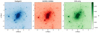 |
Fig. 1. Simulated convergence maps of a cluster lens, namely with ID = 4, at zl = 0.22 and considering zs = 3, obtained by collapsing the total mass along the z-projection. The left and the central panels show the results using two different hydro-solvers GadgetX and GIZMO-SIMBA, respectively. In the right panel, we display the convergence map of the same cluster projection simulated using only collisionless dark matter particles, DM-only run. The assumed field of view is 5 Mpc by side, collapsing ±5 Mpc matter along the line-of-sight. |
From the convergence κ, we can write the lensing potential ψ, from the two-dimensional Poisson equation, as:
 (4)
(4)
that we numerically solve in Fourier space using the Fast Fourier Transform (FFT) method. From Eq. (4), we can detail the two components (γ1, γ2) of the pseudo-vector shear, as:
 (5)
(5)
 (6)
(6)
where x and y represent the two components of the vector θ.
We use these equations to build shear maps that are then analysed in the next sections. For each cluster, we use the shear maps to simulate an observed surface mass density profile, ΔΣ, by randomly sampling the field of view with a given number density of expected background sources. Notice that the real observable is the reduced shear, g = γ/(1 − κ), which, in the weak lensing regime, we can approximate as g ≃ γ. We assume a background density of sources for weak lensing normalised to the total value of 30 galaxies per square arcmin, with a peak around z = 1 (Boldrin et al. 2012, 2016; Euclid Collaboration: Giocoli et al. 2024). The excess surface mass density, ΔΣ, shown in Fig. 2 is defined as  , with
 (7)
(7)
where (0, 0) is the centre of the cluster by construction,  and ϕi = arctan(yi/xi).
The associated error bars account for the intrinsic shape of the background galaxies and the uncertainty on the mean value within the annulus (see Euclid Collaboration: Giocoli et al. 2024), which can be read as:
 (8)
(8)
where σe = 0.3 (Hoekstra et al. 2004, 2011; Kilbinger 2015; Euclid Collaboration: Blanchard et al. 2020) is the dispersion of the shape of background source galaxies, and θ1 and θ2 are the lower and upper bounds of the considered radial annulus. From Fig. 2, we observe that for this specific cluster, the run performed with the GadgetX code has a higher excess surface mass density than the other runs (GIZMO-SIMBA and DM-only) as evident from the bottom sub-panel of the figure.
2.3. Profile model
In order to model the simulated weak-lensing profile, we adopt a smoothly truncated NFW density profile (BMO, Baltz et al. 2009), defined as:
 (9)
(9)
with Rt = t R200 with t defined as the truncation factor. Following the results by Oguri & Hamana (2011), Bellagamba et al. (2019), and Giocoli et al. (2021), we adopt a truncation radius Rt = 3 R200. The total mass enclosed within R200, M200, can be thought of as the normalisation of the model and as a mass proxy of the true enclosed mass of the DM halo hosting the cluster (Giocoli et al. 2012b). Writing r3D2 as the sum in quadrature between the sky projected coordinate r = Ddθ and the line-of-sight ζ coordinate, and integrating along ζ, we can write
 (10)
(10)
The differential excess surface mass density can then be written as:
 (11)
(11)
In order to model the data, we performed a Bayesian analysis using Monte Carlo Markov Chain approach, assuming a Gaussian log-likelihood between the model and the data2 (Marulli et al. 2016) that can be read as:
 (12)
(12)
where
 (13)
(13)
and the sum extends to the number of radial bins. We set uniform priors for log(M200/[h−1 M⊙]) ∈ [12.5, 16] and c200 ∈ [1, 15], and let each MCMC chain run for 16 000 steps.
In our simulated weak-lensing analyses, we assume a diagonal covariance matrix, neglecting off-diagonal contributions that arise in real observations. This assumption is motivated by the fact that, in a controlled simulation setting, we primarily account for shape noise as the dominant source of uncertainty. Off-diagonal terms in the covariance matrix are typically introduced by correlated large-scale structure (LSS) along the line of sight (Hoekstra et al. 2013; Gruen et al. 2015), sample variance (Singh et al. 2017), and survey-specific systematics (MacCrann et al. 2022). These effects contribute significantly to the uncertainty in cluster mass estimates but are absent in our idealised approach, which isolates weak-lensing signal uncertainties from observational complexities. While real weak-lensing analyses incorporate these additional sources of covariance, leading to significant off-diagonal terms (Schneider et al. 2002, 2022; Takada & Bridle 2007), our simulations focus on an idealised scenario where such contributions are not explicitly modelled. This allows for a clearer interpretation of the primary sources of statistical uncertainty while avoiding biases introduced by imperfect modelling of LSS or systematic effects. Nevertheless, it is important to acknowledge that omitting off-diagonal terms may lead to an underestimation of the total uncertainty in weak-lensing mass estimates (Hoekstra 2003). Future work incorporating more realistic simulations, including correlated LSS structures and survey-dependent systematics, will be necessary to fully quantify these effects.
In Fig. 2, the solid curves show the best-fit result as the model computed from the median values of the posterior distributions for the same considered cluster as in the previous figure. The bottom sub-panel displays the relative difference between the excess surface mass density measured – and modelled – in the hydro runs versus the DM-only case. From the figure, we can observe that the GadgetX simulated clusters present a steepening towards the centre, 10% larger than the other two cases. In contrast, the hydro run GIZMO-SIMBA profile is quite close to the DM-only one.
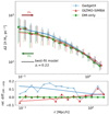 |
Fig. 2. Excess surface mass density profile of the projections displayed in Fig. 1. The colours used for the data points, blue, red and green, correspond to the GadgetX, GIZMO-SIMBA and DM-only run, respectively. The bottom panel displays the relative difference with respect to the DM-only case. The best-fit models are shown using solid curves, coloured according to each considered case. |
In Fig 3, we show the posterior distributions of the derived mass and concentration. We compare our results with respect to the parameters of the DM-only cluster. In particular, while all derived masses are consistent within 1σ uncertainties with respect to the run with only dark matter (dashed vertical line), the concentration of the GadgetX run turns out to be more than 1σ away from the DM-only case (dashed horizontal line), as a consequence of the steeper projected profile towards the centre, as displayed in Fig. 2.
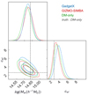 |
Fig. 3. Posterior distributions of derived weak-lensing mass and concentration from the three weak-lensing simulations of the cluster of Fig. 1 and Fig. 2. The dashed lines indicate the three-dimensional mass and concentration for the DM-only cluster run. |
In Fig. 4, we now consider all z = 0.22 maps and show the average weak-lensing mass bias for all cluster projections with respect to either their corresponding true mass (on the left) or the true mass as measured in the DM-only simulation (on the right), this latter typically used in the halo mass function calibration (Sheth & Tormen 1999; Tinker et al. 2008; Despali et al. 2016). The right sub-panels show the PDF of the data of the three sets of simulations, while the top ones show the average relative uncertainties as a function of the corresponding rescaled mass; the bottom panels present the relative differences with respect to the DM-only mass biases. From the left figure, we see that despite the differences among the three simulation sets, they all provide the same answer for the weak-lensing bias and its scatter. From the right figure, when we compare the hydro weak-lensing masses with the DM-only masses, we find that, on average, the two hydro-runs show a specular trend, reflecting the results from the single cluster illustrated in the previous figures. While the GadgetX weak-lensing masses reduce the DM-only bias, the GIZMO-SIMBA ones tend to be larger for smaller systems. Both codes have differences that tend to vanish when M200, DM ≳ 1015 h−1 M⊙, as displayed in the bottom sub-panel. This result and its dependence on the mass is linked to the fact that even starting from the same initial condition, GIZMO-SIMBA produces groups which are less massive than Gadget-X since its strong feedback pushes out a large fraction of the gas mass and thus slow down the overall matter accretion.
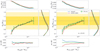 |
Fig. 4. Average weak-lensing mass biases as a function of the corresponding three-dimensional masses. On the left, the weak lensing masses are relative to their respective total mass; on the right, they are always related to the total mass of the DM-only runs. The top and bottom sub-panels show the mean relative uncertainties and the relative differences with to the DM-only case as a function of considered three-dimensional reference mass, respectively. The right panels display the distribution of the weak-lensing mass biases over all cluster masses. The dark and light yellow bands show the 10% and 20% differences, respectively. |
Euclid Collaboration: Giocoli et al. (2024) have presented the average cluster weak-lensing mass biases as a function of redshift, using the results of the GadgetX simulations. To complement their findings, in Fig. 5, we show the average weak-lensing mass biases with respect to the dark matter-only simulation mass as a function of redshift for the three simulation runs. In order to underline the dependence on the halo mass at each redshift, we split the cluster sample into two subsamples, containing clusters with M200, DM larger or smaller than 5 × 10¹⁴ h−1 M⊙. We colour-code the results by the DM-only mass. In general, we note that more massive clusters suffer from a smaller WL mass bias, as underlined by Euclid Collaboration: Giocoli et al. (2024), depending on the weak lensing signal-to-noise, modulated by the considered source redshift distribution. It is also worth mentioning that the GadgetX and GIZMO-SIMBA clusters have an opposite trend with respect to the DM-only simulation: while the former ones are on average higher by 1.2% (1.6%), the latter are ones lower by 1.2% (3.7%), for the more massive (less massive) clusters with M200, DM ≥ 5 × 10¹⁴ h−1 M⊙ (M200, DM < 5 × 10¹⁴ h−1 M⊙), respectively. The dotted lines display the redshift evolution of the mass biases with respect to the considered three-dimensional hydrodynamical, again underlining that, in this case, the differences with respect to the corresponding true mass are only within a few per cent, between different simulations.
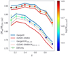 |
Fig. 5. Average weak-lensing mass biases as a function of redshift. Data points with error bars, colour-coded according to their DM-only corresponding mass, show the dark matter-only run results. Blue and red lines refer to the GadgetX and GIZMO-SIMBA hydro simulation cases, respectively. Dotted and solid lines show the bias in relation to the hydro mass and the DM-only mass, respectively. |
Before concluding this section, it is worth noticing that Lee et al. (2018) have underlined that the biases at small masses could be driven by the concentration priors and the anti-correlation correlation between concentration and mass; moreover, while Euclid Collaboration: Ragagnin et al. (2025) highlighted that this could be due to the poor NFW-fit for those systems, Giocoli et al. (2014) and Euclid Collaboration: Giocoli et al. (2024) emphasised that the weak lensing signal-to-noise ratio and halo triaxiality could play the important role.
3. Weak-lensing mass-richness relations
A key approach to improving mass estimates for large cluster samples is to use the weak-lensing mass–richness relation, where richness – typically defined as the number of satellite galaxies in a cluster above a given luminosity or stellar mass threshold in a considered aperture – acts as an indirect proxy for total mass. However, translating richness into an accurate mass estimate requires thorough calibration, as richness measurements are affected by selection effects, projection biases and photometric redshift uncertainties. Dedicated simulations are crucial for quantifying and correcting these biases to ensure accurate cosmological constraints from cluster counts. In particular, richness estimates are affected by interloping galaxies falsely assigned to clusters due to projection along the line of sight. Simulations can model these effects, enabling corrections for contamination and biases in richness measurements. In addition, the weak-lensing mass–richness relation may evolve with redshift, as well as the scatter, due to changes in galaxy populations, merger activity, or dynamical relaxation timescales. Simulations allow for the testing of redshift-dependent scaling parameters to ensure accurate extrapolations in high-redshift cluster studies.
This section presents the weak-lensing mass-richness relation in our simulated mass-selected cluster sample.
Weak-lensing mass-observed richness relation parameters.
We compute the cluster richness using the position of haloes and subhaloes in the simulated field of view of 5 Mpc on the side. Specifically, from each halo projection, we count the total number of subhaloes and haloes in a cylinder with a radius equal to R200, with respect to the cluster centre and height equal to ΔH = 10 Mpc that corresponds to roughly Δz = 0.002 × (1 + z), which represents an optimistic case reachable with spectroscopic data (Laureijs et al. 2011; Jauzac et al. 2021; Caminha et al. 2023; D’Addona et al. 2024; Mainieri et al. 2024). The richness of the simulated clusters is computed by considering a minimum stellar mass cut mimicking the observational measure that depends on the survey depth and the corresponding magnitude limit of the data set, photometric properties, and stellar mass determination.
In Fig. 6, we show the convergence map, haloes and subhaloes in the (x, y) plane of our test halo at redshift z = 0.22 from Fig. 1. Black circles show the location of cluster subhaloes, the red-filled triangles all haloes in the cylinder projected within R200 including also the main halo. In this case, we consider all (sub)haloes with Mstar > 0. The magenta crosses mark the haloes in a cylindrical ring between 2 and 3.5 times R200. These are chosen far enough from the cluster to be representative of the halo projected density in the field. This sample is used to estimate the number of contaminant haloes by subtracting the local background to correct the cluster richness (Andreon & Bergé 2012), which we define as:
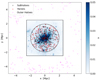 |
Fig. 6. Halo and subhalo distribution in the projection x-y considering a field of view of 10 Mpc on a side and ±5 Mpc along the line of sight, ΔH = 10 Mpc, for the GadgetX cluster run. Black circles show the location of the centre of all subhaloes within the halo radius R200, red triangles are all haloes which, in projection, fall within the halo radius, and magenta crosses are all haloes that, in projection, lie in a ring between 2 and 3.5 R200, which we term outer haloes. The blue map is the corresponding region where we simulate the weak-lensing cluster signal. |
 (14)
(14)
The geometrical factor 4/33 has been computed by rescaling the density of haloes in the cylindrical ring between 2 and 3.5 R200 to account for the difference in area. This richness estimate is computed individually for each cluster projection, while for each cluster, the intrinsic richness is calculated from λint = nSubhaloes + 1, by counting the number of satellite galaxies in subhaloes within R200, plus the central.
As reference cases, in Fig. 7, we display the weak-lensing mass versus the richness for clusters at z = 0.22 simulated using the GadgetX prescription. In the four panels we consider different stellar mass cuts, from Mstar, min = 1010 h−1 M⊙ to Mstar, min = 1010.75 h−1 M⊙ with a step dlog(Mstar, min) = 0.25. For each Mstar, min case, we display three different sets of data points. The first one is the true mass-intrinsic richness relation that considers the true M200 and all subhaloes within R200 (magenta triangles, as in Chen et al. 2024); in this case, there are no projection effects when counting the member galaxies, while bias and uncertainties on the cluster mass are set to zero. Second, combining all three cluster projections, the green circles show the case where we consider all satellite galaxies in a sphere of radius R200, plus the central, and adopt as cluster mass Mwl, the one computed modelling the weak-lensing simulated data. Third, the blue-filled circles, with the corresponding error bars, show the observed richness with the corresponding Poisson uncertainty and the weak-lensing mass Mwl, calculated as described in Section 2.3. For comparison, in the top two panels, the magenta dashed lines show the results by Chen et al. (2024), who modelled the intrinsic cluster richness as a function of the true mass M200, calibrated up to Mstar, min ≃ 1010 h−1 M⊙, using the same simulations of this work. Note that this model already fails to describe the magenta triangle in the top-right panel for which Mstar, min = 1012.5 h−1 M⊙. In all panels of Figure 7, we show two log-log relations between mass and richness described here calculated for different minimum stellar mass cuts used in computing the richness. Notice that the scatter increases at higher stellar mass cuts and that the inverse relation (displayed with a dot-dashed orange line) differs from the weak-lensing mass-richness relation when the scatter and the errors in the richness are larger. Notice that considering that our cluster sample is a true mass-selected at z = 0, those results are not strongly affected by Malmquist-Eddington biases. For redshift z > 0, the low mass sample is modulated by the stochasticity of the mass accretion history (van den Bosch 2002; Giocoli et al. 2007, 2012c) and by the noisy estimate of the mass via weak lensing simulations, and the corresponding uncertainties.
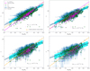 |
Fig. 7. Weak-lensing mass-observed richness relation measured for the clusters at redshift z = 0.22 run with GadgetX. The different panels consider different minimum stellar mass cuts Mstar, min, from 1010 to 1010.75 h−1 M⊙. The weak-lensing masses Mwl are rescaled with respect to the pivot value Mp = 3 × 10¹⁴ h−1 M⊙. The blue points with the corresponding error bars show the results for the observed richness calculated as in Eq. (14) and the derived weak-lensing mass from the tangential shear profile. For the magenta triangles, the mass is not Mwl, but M200; correspondingly we show the number λint of galaxies within R200. The green circles show the results when using Mwl and the number of subhaloes in a sphere with radius R200. The solid blue line displays the results of our fit performed using MCMC on the blue data points, and in cyan, the 1σ uncertainty. The orange dash-dotted line is the best fit of the inverse relation; see Eq. (18). Black dotted lines display the model presented in this work, WLOR relation as in Eq. (15) considering the values reported in Table 1. |
-
Weak-lensing mass-observed richness relation
The solid blue lines display the best result of the linear regression model:
 (15)
(15)
where masses are rescaled with respect to the pivot value Mp = 3 × 10¹⁴ h−1 M⊙, the intercept A and the slope B are computed using an MCMC Bayesian inference model, assuming a Gaussian likelihood. The latter, accounting for error bars on both axes is written as:
![Mathematical equation: $$ \begin{aligned} \mathcal{L} \propto \exp \left\{ - \dfrac{1}{2} \sum _i \left[\dfrac{ \log \left(\lambda _{\mathrm{obs},i}\right) -\log \left(\lambda _i\right)}{ \sigma _i}\right]^2 \right\} , \end{aligned} $$](/articles/aa/full_html/2025/05/aa53871-25/aa53871-25-eq22.gif) (16)
(16)
with
 (17)
(17)
where σlog λobs, i and σlog Mwl, i are the uncertainties relative to the i-cluster. Notice that we assume a Poisson uncertainty to the richness with  . We assume wide uniform priors for A and B: A ∈ [ − 50, 50] and B ∈ [ − 1; 5]. The cyan-shaded regions in Fig. 7 display the 1σ uncertainty of the linear regression model parameters. The observed richness is related to the weak-lensing mass by a power-law relation
  , and considering that both observables have their corresponding associated uncertainties, it follows that
  (Andreon 2010, 2012, 2016; Andreon & Bergé 2012; Andreon & Hurn 2013).
-
Observed richness-weak-lensing mass relation
The orange dash-dotted lines in Fig. 7, display the inverse of the median posteriors of the linear regression:
 (18)
(18)
that relates the weak-lensing mass to the observed richness by the power-law relation  , underlining that D ≠ 1/B. For likelihood modelling of the linear regression parameters C and D, we use Equation (16) substituting the richness with the mass, the associated uncertainty propagation can be read as
 (19)
(19)
While Figure 7 refers only to GadgetX, in the two panels of Fig. 8, we show the weak-lensing mass-observed richness (WLOR) relation in both hydro-runs, considering the two largest stellar mass cuts: GadgetX in blue and GIZMO-SIMBA in red, respectively. The results of the linear regression Bayesian inferred model are shown with the corresponding coloured solid lines and the shaded 1σ uncertainty. The figure shows that the results from both hydro runs are consistent within the shaded uncertainty region derived from the independent propagated uncertainties in the MCMC analyses of the two hydro runs. The right sub-panels show the PDF of the scatter of the observed richness with respect to the corresponding linear regression model at a fixed weak-lensing mass, with the shaded region marking the corresponding scatter σlog λobs. It is worth underlining that, on average, the scatter in the GIZMO-SIMBA cluster simulations is marginally larger than the one measured in GadgetX. Generally, the parameters A and B of the linear regression model (see Eq. (15)) and derived σlog λobs depend on the stellar mass cut Mstar, min, redshift z and the hydro simulation considered.
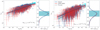 |
Fig. 8. Weak-lensing mass-observed richness relation measured for the clusters at redshift z = 0.22 run with both hydrocodes GadgetX in blue and GIZMO-SIMBA in red, respectively. The blue points are thus the same from Figure 7. The solid lines show the linear regression model results, with the shaded region indicating the 1σ uncertainty on the intercept and slope parameters. In each sub-figure – where we consider two different stellar mass cuts when computing λobs, the right sub-panel shows the PDF of the scatter of the observed richness (using a Gaussian KDE) with respect to the best-fit linear regression model; the shaded bands mark the corresponding 1σ deviation: σlog λ. |
3.1. Redshift evolution
Our analysis aims to model the observed richness-weak-lensing mass relations for clusters at different redshifts from z = 0.12 up to z = 0.94. In order to do so, we model all the nine considered simulation snapshots and analytically describe the redshift evolution of the parameters describing this scaling relation, namely the intercept, the slope and the scatter.
We summarise the results of the WLOR parameters in Fig. 9, where they are displayed as a function of the cluster redshifts, the four considered stellar mass cuts and both hydro runs – in blue and red for the GadgetX and GIZMO-SIMBA, respectively. We note that the intercept A is consistent with being redshift independent and increasing with the stellar mass cut. GadgetX clusters have slightly larger values than the GIZMO-SIMBA ones. The slope parameter B and the derived scatter σlog λobs instead manifest a moderate redshift dependence. A second-order polynomial a + b z + c z2, fixing c = −0.42 independently of the stellar mass cut, describes quite well the slope, while the scatter is well fit by a linear relation. In particular, the WLOR relations of the GadgetX clusters have a steeper slope B than the GIZMO-SIMBA ones. Notice that the slope parameter is relatively constant up to z ≃ 0.55, after which we are sensitive to the variation and the cut-off of the stellar mass function (Chen et al. 2024) reflecting the complex interplay between galaxy formation, environmental effects, and hierarchical structure formation. The black lines and curves in the three panels, styled according to the different considered minimum stellar mass cuts Mstar, min, represent the best-fit models combining both hydro-runs. In Table 1, we summarise the best-fit parameters of redshift evolution and for different stellar mass cuts. The dotted black lines – labelled as ‘This work’ or as ‘This work Mwl’ – reported in the Figs. 7, 8 and 11 have been computed adopting the best-fit model parameters as reported in Table 1. We follow the same procedure, combining the results of both hydro simulations to model the redshift evolution of the parameters of the observed richness-weak-lensing mass (ORWL) relation C, D and the derived scatter σlog Mwl, as reported in Table 2.
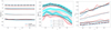 |
Fig. 9. Intercept A, slope B, and scatter σlog λobs at a fixed weak-lensing cluster mass as a function of redshift. Blue and red curves refer to the two hydro simulations: GadgetX and GIZMO-SIMBA, respectively. In all panels, the results referring to a given stellar mass cuts are reported with different line styles. The black curves show the best-fit models as a function of redshift, combining both hydro run results at a fixed stellar mass cut. The best-fit values are reported in Table 1. |
Observed richness-weak lensing mass relation parameters.
It is worth underlining that we also retrieved the ORWL relation by adopting sharp richness cut, both in λobs and λtrue, to further test that the Malmquist-Eddington biases do not affect our results. We used severe λcut > [100, 60, 20, 10] for the four Mstar, min-cut samples, respectively, finding linear regressions slightly steeper but fully consistent with our reference results within the 1σ confidence region.
3.2. Comparison with the literature
In Fig. 10, we compare our ORWL relation – considering Mstar, min = 1010 h−1 M⊙ – with results from previous studies, rescaling various redMaPPer richnesses following Table 5 of McClintock et al. (2019).
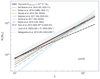 |
Fig. 10. Observed richness-weak-lensing mass relation comparison with different literature results. We compute our model considering an observed richness with a minimum stellar mass of Mstar, min = 1010 h−1 M⊙ and the parameters have been calculated at z = 0.35. All redMaPPer (Rykoff et al. 2014) richness definitions have been rescaled to DES-Y1 by McClintock et al. (2019) (see their Table 5). The two dotted lines referring to KiDS-DR3 clusters from Lesci et al. (2022a) and Bellagamba et al. (2019) have been computed with the AMICO cluster finder algorithm (Maturi et al. 2019). |
McClintock et al. (2019) constrained the richness-mass scaling relation for galaxy clusters in DES Year 1 data using weak lensing, dividing clusters into richness (λ ≥ 20) and redshift (0.2 ≤ z ≤ 0.65) bins. Mean masses were measured via stacked lensing signals, and their analysis, incorporating detailed systematic error considerations, provided precise constraints, demonstrating DES’s potential for cluster cosmology.
Baxter et al. (2018) used CMB lensing from SPT and DES Year 1 clusters (with mean redshift z = 0.45), constraining the mass-richness relation with ∼17% precision. Their analysis was primarily limited by statistical noise, with notable systematics from the thermal SZ effect and cluster miscentering. Simet et al. (2017) and Murata et al. (2018) constrained the mass-richness relation for SDSS redMaPPer clusters in the redshift range 0.10 ≤ z ≤ 0.33, though their methodologies differed: Simet et al. (2017) applied an analytical model, while Murata et al. (2018) used forward modelling with a calibrated N-body emulator.
Melchior et al. (2017) analysed the richness-weak-lensing mass relation for over 8 000 redMaPPer clusters in DES Science Verification (SV) data, incorporating models that address systematic uncertainties. Their work extends the calibrated redshift range for redMaPPer clusters (0.3 ≤ z ≤ 0.8) while agreeing with prior weak-lensing calibrations. Mantz et al. (2016) constrained the scaling relation between redMaPPer richness and weak-lensing masses for an X-ray-selected sample from the Weighing the Giants project. Saro et al. (2015) cross-matched SPT-SZ and DES-SV clusters, confirming general consistency but identifying mild tensions in expected matching rates. They found that optical-SZE positional offsets followed a bimodal distribution.
Bellagamba et al. (2019) and Lesci et al. (2022a) adopted AMICO, an alternative optical cluster finder that does not rely on colour-based selection, reducing biases from red-sequence detection. AMICO leverages galaxy luminosity, spatial distribution, and photo-z data to provide probabilistic galaxy-cluster associations. Purity and completeness are evaluated using mock catalogues derived directly from observational data, avoiding reliance on numerical or semi-analytic models (Maturi et al. 2019). While Bellagamba et al. (2019) constrained the AMICO richness-mass relation using a stacked cluster sample, Lesci et al. (2022a) included a model for the redshift evolution of the cluster mass function.
The redMaPPer algorithm identifies clusters using the red sequence, assuming a dominant population of red, passively evolving galaxies. In contrast, AMICO relies on galaxy luminosity, spatial distribution, and photometric redshifts, making it independent of galaxy colour. For richness estimation, redMaPPer uses a probability-based approach focused on red-sequence galaxies, whereas AMICO probabilistically incorporates all galaxies, considering spatial and magnitude constraints without colour dependence. This key distinction leads to differences in observed cluster populations, as shown in Fig. 10.
From a numerical simulation perspective, selecting galaxies based solely on a stellar mass threshold better aligns with redMaPPer’s richness definition. This is represented by the solid black line in Fig. 10, while the shaded region denotes σlog M as modelled in The Three Hundred clusters (Table 2). With a few exceptions, our simulated ORWL relation agrees well with observational data, particularly for richness λ ≥ 30.
Before concluding this section, it is worth mentioning also the results from the CODEX clusters (Finoguenov et al. 2020). Phriksee et al. (2020), for the low redshift sample, found a slope equal to unity, while Kiiveri et al. (2021) recovered a shallower slope in the mass-richness plane than McClintock et al. (2019).
4. True mass-richness relations
The observed richness could also be directly used as a true mass proxy. In order to calibrate the relation with the true mass of the cluster, it is worth underlining that for each cluster, we have three observed richness estimates, depending on the projection we are looking at, and one true mass M200 defined as the spherical mass within the radius R200 which encloses 200 times the critical comoving density of the universe ρc(z) at the considered redshift. We model the linear regression between M200 and λobs, and at different redshifts, using the same methodology of the previous section. In our MCMC analysis, we adopt the same likelihood as in Eqs. (16) and (17), neglecting the uncertainty on the mass and considering only the Poissonian error on the observed richness.
In Fig. 11, we display the true mass-observed richness relation for clusters at z = 0.22 for both hydro-runs and the two highest stellar mass cuts. In both panels, the blue and red solid lines display the best-fit linear regression models computed from the median parameters of the posterior distributions. Since, in this case, we have the uncertainty only on the y-axis, we can directly invert λobs ∝ M200B into  . The black dotted lines in the figure represent the linear regression models adopting the best-fit parameters as in Table 1, as computed for the observed richness-weak-lensing mass relation. The dot-dashed magenta lines represent the linear regression model for the observed richness-true mass case, the parameters of which are summarised in Table 3, obtained by combining the results of both hydro-runs. From the figure, we observe that, on average, the difference between the black dotted and magenta dot-dashed lines reflects the weak-lensing mass bias as described in detail by Euclid Collaboration: Giocoli et al. (2024): the weak-lensing mass of low mass clusters is, on average, more biased low than that of high mass systems with respect to the true cluster mass. Notice that the difference between the black-dotted and the dot-dashed magenta is also guided by the dispersion of the observed richnesses.
True mass-richness relation parameters.
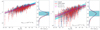 |
Fig. 11. True mass-observed richness relation for the clusters at redshift z = 0.22 as measured in both hydro-runs. The solid lines show the linear regression model results, with the shaded region indicating the 1σ uncertainty on the intercept and slope parameters. In each sub-figure, the right sub-panel shows the probability distribution function of the λobs with respect to the corresponding best-fit linear model, with the shaded regions marking the corresponding scatter σlog λobs. The dotted black lines exhibit the model for the richness weak-lensing mass relation, as described in the last section. |
As previously discussed, we model the evolution of the intercept A, the slope B and the derived scatter σlog λobs as a function of redshift and for the four considered stellar mass cuts, in the true mass-observed richness relation. We also note that, in this case, the intercept is redshift-independent, the slope has a second-order polynomial dependence on z but with the second-order term coefficient c = −0.18 and the scatter of the observed richness at a given true mass M200 depends linearly with redshift. It is worth underlining that the scatter of the observed richness at a fixed true mass is smaller than that of a fixed weak-lensing mass at a given redshift and stellar mass cut, as expected being Mwl a noisy proxy of the true underlying mass.
5. Summary and conclusions
Cosmological numerical simulations play an important role in guiding cluster cosmology studies. Weak gravitational lensing is the leading method in reconstructing galaxy clusters’ projected matter density distribution. However, derived weak-lensing masses are biased low with respect to the true tridimensional mass, which is used in the halo mass function models.
Using state-of-the-art hydrodynamical simulations, in this work, we quantify the average weak-lensing bias dependences of two hydro-solvers GadgetX and GIZMO-SIMBA and compare with respect to a DM-only one (Tinker et al. 2008; Sheth & Tormen 1999; Despali et al. 2016). Using cluster random projections, we also calibrate the weak-lensing mass-richness relation and its inverse and compare our findings with different literature results. In what follows, we summarise our main results:
-
All weak-lensing masses are, on average, negatively biased with respect to the corresponding true mass (Meneghetti et al. 2007, 2010a,b; Lee et al. 2018). While the ratio between the weak-lensing masses of GadgetX clusters and the three-dimensional DM-only ones are a few per cent higher, the ones derived from GIZMO-SIMBA are lower probably due to the shallower inner slope of the total density profile due to the strong AGN feedback (Meneghetti et al. 2023); when WL masses are rescaled with respect to the corresponding three-dimensional ones all runs provide the same answer for the weak lensing mass bias and its scatter and their redshift evolution.
-
Using halo and subhalo projected positions, we derive the observed richness accounting for local background contaminants.
-
The weak-lensing mass-observed richness relations derived from both hydrodynamical simulations are consistent within 1σ because of the propagated uncertainties; accordingly, we average the linear regression parameters from these simulations in our final model.
-
While the intercept parameter is redshift-independent and varies with the minimum stellar mass cut used to define the cluster richness, the slope, almost constant up to redshift z = 0.55, changes with redshift following a second-order polynomial.
-
The redshift evolution of the scatter of the observed richness (weak-lensing mass) at a fixed weak-lensing mass (observed richness) linearly increases with redshift, and the stellar mass cut Mstar, min.
-
Our model for observed richness-weak-lensing mass is in good agreement with different literature results based on SDSS redMaPPer clusters when considering a minimum stellar mass cut Mstar, min = 1010 h−1 M⊙.
-
In our last section, we derive the linear regression parameters and their dependence on z and Mstar, min for the true mass-observed richness relation; we find that the scatter of λobs at a given true mass is smaller than the scatter at a given weak-lensing mass.
Numerical simulations have been extensively used to model the cluster mass function as a function of redshift and overdensity, along with their dependence on cosmology. However, the three-dimensional overdensity mass of clusters is not directly observable, and its reconstruction requires high-quality data and calibration with advanced numerical simulations. By combining this with other mass proxies obtained from multi-band observations, well-calibrated mass-observable relations can be developed to estimate galaxy cluster masses for larger samples with known observable properties. To conclude, it is important to underline that establishing and quantifying the relationship between weak-lensing cluster mass, richness and potential systematics from baryonic physics is crucial for advancing precision cluster cosmology studies.
Acknowledgments
LM and CG acknowledge the financial contribution from the PRIN-MUR 2022 20227RNLY3 grant ‘The concordance cosmological model: stress-tests with galaxy clusters’ supported by Next Generation EU and from the grant ASI n. 2024-10-HH.0 “Attività scientifiche per la missione Euclid – fase E”. GC thanks the support from INAF theory Grant 2022: Illuminating Dark Matter using Weak Lensing by Cluster Satellites. GD acknowledges the funding by the European Union – NextGenerationEU, in the framework of the HPC project – “National Centre for HPC, Big Data and Quantum Computing” (PNRR – M4C2 – I1.4 – CN00000013 – CUP J33C22001170001). SB is supported by the Fondazione ICSC, Spoke 3 Astrophysics and Cosmos Observations. National Recovery and Resilience Plan (Piano Nazionale di Ripresa e Resilienza, PNRR) Project ID CN00000013 “Italian Research Center on High-Performance Computing, Big Data and Quantum Computing” funded by MUR Missione 4 Componente 2 Investimento 1.4: Potenziamento strutture di ricerca e creazione di “campioni nazionali di R&S (M4C2-19 )” – Next Generation EU (NGEU); the National Recovery and Resilience Plan (NRRP), Mission 4, Component 2, Investment 1.1, Call for tender No. 1409 published on 14.9.2022 by the Italian Ministry of University and Research (MUR), funded by the European Union – NextGenerationEU– Project Title “Space-based cosmology with Euclid: the role of High-Performance Computing” – CUP J53D23019100001 – Grant Assignment Decree No. 962 adopted on 30/06/2023 by the Italian Ministry of Ministry of University and Research (MUR). GC, GD, MM, LM, SB and FM are also supported by the INFN InDark Grant. This research was supported in part by grant NSF PHY-2309135 to the Kavli Institute for Theoretical Physics (KITP). The authors acknowledge The Red Española de Supercomputación for granting computing time for running most of the simulations of The Three Hundred galaxy cluster project in the Marenostrum supercomputer at the Barcelona Supercomputing Center. WC and GY would like to thank Ministerio de Ciencia e Innovación for financial support under project grant PID2021-122603NB-C21. WC is also supported by the STFC AGP Grant ST/V000594/1 and the Atracción de Talento Contract no. 2020-T1/TIC-19882 granted by the Comunidad de Madrid in Spain. He also thanks the ERC: HORIZON-TMA-MSCA-SE for supporting the LACEGAL-III project with grant number 101086388 and the China Manned Space Project for its research grants. This work has been made possible by the ‘The Three Hundred’ collaboration (https://www.nottingham.ac.uk/astronomy/The300/index.php).
References
- Abbott, T. M. C., Aguena, M., Alarcon, A., et al. 2020, Phys. Rev. D, 102, 023509 [Google Scholar]
- Abbott, T. M. C., Aguena, M., Alarcon, A., et al. 2022, Phys. Rev. D, 105, 023520 [CrossRef] [Google Scholar]
- Adame, A. G., Aguilar, J., Ahlen, S., et al. 2025, JCAP, 2025, 021 [CrossRef] [Google Scholar]
- Andreon, S. 2010, MNRAS, 407, 263 [NASA ADS] [CrossRef] [Google Scholar]
- Andreon, S. 2012, A&A, 548, A83 [NASA ADS] [CrossRef] [EDP Sciences] [Google Scholar]
- Andreon, S. 2016, A&A, 587, A158 [NASA ADS] [CrossRef] [EDP Sciences] [Google Scholar]
- Andreon, S., & Bergé, J. 2012, A&A, 547, A117 [NASA ADS] [CrossRef] [EDP Sciences] [Google Scholar]
- Andreon, S., & Hurn, M. 2013, Stat. Anal. Data Min.: ASA Data Sci. J., 9, 15 [Google Scholar]
- Ansarinejad, B., Raghunathan, S., Abbott, T., et al. 2024, J. Cosmol. Astropart. Phys., 2024, 024 [Google Scholar]
- Arthur, J., Pearce, F. R., Gray, M. E., et al. 2017, MNRAS, 464, 2027 [Google Scholar]
- Bahcall, N. A., Fan, X., & Cen, R. 1997, Am. Astron. Soc. Meet. Abstr., 190, 52.01 [Google Scholar]
- Baltz, E. A., Marshall, P., & Oguri, M. 2009, JCAP, 2009, 015 [Google Scholar]
- Bartelmann, M. 2010, Classical Quantum Gravity, 27, 233001 [NASA ADS] [CrossRef] [Google Scholar]
- Bartelmann, M., & Schneider, P. 2001, Phys. Rep., 340, 291 [Google Scholar]
- Baxter, E. J., Raghunathan, S., Crawford, T. M., et al. 2018, MNRAS, 476, 2674 [Google Scholar]
- Beck, A. M., Murante, G., Arth, A., et al. 2016, MNRAS, 455, 2110 [Google Scholar]
- Becker, M. R., & Kravtsov, A. V. 2011, ApJ, 740, 25 [NASA ADS] [CrossRef] [Google Scholar]
- Bellagamba, F., Sereno, M., Roncarelli, M., et al. 2019, MNRAS, 484, 1598 [Google Scholar]
- Benitez-Llambay, A. 2015, http://dx.doi.org/10.5281/zenodo.21703 [Google Scholar]
- Bergamini, P., Acebron, A., Grillo, C., et al. 2023, ApJ, 952, 84 [NASA ADS] [CrossRef] [Google Scholar]
- Bocquet, S., Grandis, S., Bleem, L. E., et al. 2024a, Phys. Rev. D, 110, 083509 [NASA ADS] [CrossRef] [Google Scholar]
- Bocquet, S., Grandis, S., Bleem, L. E., et al. 2024b, Phys. Rev. D, 110, 083510 [NASA ADS] [CrossRef] [Google Scholar]
- Boldrin, M., Giocoli, C., Meneghetti, M., & Moscardini, L. 2012, MNRAS, 427, 3134 [NASA ADS] [CrossRef] [Google Scholar]
- Boldrin, M., Giocoli, C., Meneghetti, M., et al. 2016, MNRAS, 457, 2738 [CrossRef] [Google Scholar]
- Caminha, G. B., Grillo, C., Rosati, P., et al. 2023, A&A, 678, A3 [NASA ADS] [CrossRef] [EDP Sciences] [Google Scholar]
- Carbone, C., Fedeli, C., Moscardini, L., & Cimatti, A. 2012, JCAP, 2012, 023 [CrossRef] [Google Scholar]
- Chen, M., Cui, W., Fang, W., & Wen, Z. 2024, ApJ, 966, 227 [Google Scholar]
- Costanzi, M., Sartoris, B., Viel, M., & Borgani, S. 2014, JCAP, 10, 081 [Google Scholar]
- Costanzi, M., Saro, A., Bocquet, S., et al. 2021, Phys. Rev. D, 103, 043522 [Google Scholar]
- Cui, W., Power, C., Knebe, A., et al. 2016, MNRAS, 458, 4052 [Google Scholar]
- Cui, W., Knebe, A., Yepes, G., et al. 2018, MNRAS, 480, 2898 [Google Scholar]
- Cui, W., Dave, R., Knebe, A., et al. 2022, MNRAS, 514, 977 [NASA ADS] [CrossRef] [Google Scholar]
- D’Addona, M., Mercurio, A., Rosati, P., et al. 2024, A&A, 686, A4 [NASA ADS] [CrossRef] [EDP Sciences] [Google Scholar]
- Davé, R., Anglés-Alcázar, D., Narayanan, D., et al. 2019, MNRAS, 486, 2827 [Google Scholar]
- Despali, G., & Vegetti, S. 2017, MNRAS, 469, 1997 [NASA ADS] [CrossRef] [Google Scholar]
- Despali, G., Giocoli, C., Angulo, R. E., et al. 2016, MNRAS, 456, 2486 [NASA ADS] [CrossRef] [Google Scholar]
- Diego, J. M., Li, S. K., Amruth, A., et al. 2024, A&A, 689, A167 [NASA ADS] [CrossRef] [EDP Sciences] [Google Scholar]
- Dolag, K., Borgani, S., Murante, G., & Springel, V. 2009, MNRAS, 399, 497 [Google Scholar]
- Euclid Collaboration (Blanchard, A., et al.) 2020, A&A, 642, A191 [NASA ADS] [CrossRef] [EDP Sciences] [Google Scholar]
- Euclid Collaboration (Castro, T., et al.) 2023, A&A, 671, A100 [CrossRef] [EDP Sciences] [Google Scholar]
- Euclid Collaboration (Giocoli, C., et al.) 2024, A&A, 681, A67 [NASA ADS] [CrossRef] [EDP Sciences] [Google Scholar]
- Euclid Collaboration (Sereno, M., et al.) 2024, A&A, 689, A252 [NASA ADS] [CrossRef] [EDP Sciences] [Google Scholar]
- Euclid Collaboration (Ingoglia, L., et al.) 2025, A&A, 695, A280 [Google Scholar]
- Euclid Collaboration (Ragagnin, A., et al.) 2025, A&A, 695, A282 [Google Scholar]
- Feldbrugge, J., & van de Weygaert, R. 2024, ArXiv e-prints [arXiv:2405.20475] [Google Scholar]
- Finoguenov, A., Rykoff, E., Clerc, N., et al. 2020, A&A, 638, A114 [NASA ADS] [CrossRef] [EDP Sciences] [Google Scholar]
- Gianfagna, G., Rasia, E., Cui, W., et al. 2023, MNRAS, 518, 4238 [Google Scholar]
- Giocoli, C., Moreno, J., Sheth, R. K., & Tormen, G. 2007, MNRAS, 376, 977 [CrossRef] [Google Scholar]
- Giocoli, C., Meneghetti, M., Ettori, S., & Moscardini, L. 2012a, MNRAS, 426, 1558 [NASA ADS] [CrossRef] [Google Scholar]
- Giocoli, C., Meneghetti, M., Bartelmann, M., Moscardini, L., & Boldrin, M. 2012b, MNRAS, 421, 3343 [Google Scholar]
- Giocoli, C., Tormen, G., & Sheth, R. K. 2012c, MNRAS, 422, 185 [NASA ADS] [CrossRef] [Google Scholar]
- Giocoli, C., Meneghetti, M., Metcalf, R. B., Ettori, S., & Moscardini, L. 2014, MNRAS, 440, 1899 [NASA ADS] [CrossRef] [Google Scholar]
- Giocoli, C., Marulli, F., Moscardini, L., et al. 2021, A&A, 653, A19 [NASA ADS] [CrossRef] [EDP Sciences] [Google Scholar]
- Giocoli, C., Palmucci, L., Lesci, G. F., et al. 2024, A&A, 687, A79 [NASA ADS] [CrossRef] [EDP Sciences] [Google Scholar]
- Gnedin, O. Y., Kravtsov, A. V., Klypin, A. A., & Nagai, D. 2004, ApJ, 616, 16 [Google Scholar]
- Grandis, S., Mohr, J. J., Dietrich, J. P., et al. 2019, MNRAS, 488, 2041 [NASA ADS] [Google Scholar]
- Grandis, S., Bocquet, S., Mohr, J. J., Klein, M., & Dolag, K. 2021, MNRAS, 507, 5671 [NASA ADS] [CrossRef] [Google Scholar]
- Grandis, S., Ghirardini, V., Bocquet, S., et al. 2024, A&A, 687, A178 [NASA ADS] [CrossRef] [EDP Sciences] [Google Scholar]
- Gruen, D., Seitz, S., Becker, M. R., Friedrich, O., & Mana, A. 2015, MNRAS, 449, 4264 [NASA ADS] [CrossRef] [Google Scholar]
- Haggar, R., Gray, M. E., Pearce, F. R., et al. 2020, MNRAS, 492, 6074 [NASA ADS] [CrossRef] [Google Scholar]
- Hoekstra, H. 2003, MNRAS, 339, 1155 [NASA ADS] [CrossRef] [Google Scholar]
- Hoekstra, H., Yee, H. K. C., & Gladders, M. D. 2004, ApJ, 606, 67 [Google Scholar]
- Hoekstra, H., Hartlap, J., Hilbert, S., & van Uitert, E. 2011, MNRAS, 412, 2095 [NASA ADS] [CrossRef] [Google Scholar]
- Hoekstra, H., Bartelmann, M., Dahle, H., et al. 2013, Space Sci. Rev., 177, 75 [NASA ADS] [CrossRef] [Google Scholar]
- Hoosain, M., Blyth, S.-L., Skelton, R. E., et al. 2024, MNRAS, 528, 4139 [NASA ADS] [CrossRef] [Google Scholar]
- Hopkins, P. F. 2015, MNRAS, 450, 53 [Google Scholar]
- Ivezic, Z., Tyson, J. A., Abel, B., et al. 2008, ApJ, 873, 111 [Google Scholar]
- Ivezic, Z., Tyson, J. A., Axelrod, T., et al. 2009, in American Astronomical Society Meeting Abstracts c="Undefined command " l="160"/>213, BAAS, 41, 366 [Google Scholar]
- Jauzac, M., Klein, B., Kneib, J.-P., et al. 2021, MNRAS, 508, 1206 [NASA ADS] [CrossRef] [Google Scholar]
- Kiiveri, K., Gruen, D., Finoguenov, A., et al. 2021, MNRAS, 502, 1494 [NASA ADS] [CrossRef] [Google Scholar]
- Kilbinger, M. 2015, Rep. Progr. Phys., 78, 086901 [Google Scholar]
- Kleinebreil, F., Grandis, S., Schrabback, T., et al. 2025, A&A, 695, A216 [NASA ADS] [CrossRef] [EDP Sciences] [Google Scholar]
- Klypin, A., Yepes, G., Gottlöber, S., Prada, F., & Heß, S. 2016, MNRAS, 457, 4340 [Google Scholar]
- Knebe, A., Gámez-Marín, M., Pearce, F. R., et al. 2020, MNRAS, 495, 3002 [Google Scholar]
- Knollmann, S. R., & Knebe, A. 2009, ApJS, 182, 608 [Google Scholar]
- Laureijs, R., Amiaux, J., Arduini, S., et al. 2011, ArXiv e-prints [arXiv:1110.3193] [Google Scholar]
- Lee, B. E., Le Brun, A. M. C., Haq, M. E., et al. 2018, MNRAS, 479, 890 [Google Scholar]
- Lesci, G. F., Marulli, F., Moscardini, L., et al. 2022a, A&A, 659, A88 [NASA ADS] [CrossRef] [EDP Sciences] [Google Scholar]
- Lesci, G. F., Nanni, L., Marulli, F., et al. 2022b, A&A, 665, A100 [NASA ADS] [CrossRef] [EDP Sciences] [Google Scholar]
- Li, Q., Cui, W., Yang, X., et al. 2023, MNRAS, 523, 1228 [NASA ADS] [CrossRef] [Google Scholar]
- Libeskind, N. I., van de Weygaert, R., Cautun, M., et al. 2018, MNRAS, 473, 1195 [NASA ADS] [CrossRef] [Google Scholar]
- Lima, M., & Hu, W. 2005, Phys. Rev. D, 72, 043006 [NASA ADS] [CrossRef] [Google Scholar]
- MacCrann, N., Becker, M. R., McCullough, J., et al. 2022, MNRAS, 509, 3371 [Google Scholar]
- Mainieri, V., Anderson, R. I., Brinchmann, J., et al. 2024, ArXiv e-prints [arXiv:2403.05398] [Google Scholar]
- Malavasi, N., Arnouts, S., Vibert, D., et al. 2017, MNRAS, 465, 3817 [Google Scholar]
- Mantz, A. B., Allen, S. W., Morris, R. G., et al. 2016, MNRAS, 463, 3582 [NASA ADS] [CrossRef] [Google Scholar]
- Marulli, F., Veropalumbo, A., & Moresco, M. 2016, Astron. Comput., 14, 35 [Google Scholar]
- Maturi, M., Bellagamba, F., Radovich, M., et al. 2019, MNRAS, 485, 498 [Google Scholar]
- McClintock, T., Varga, T. N., Gruen, D., et al. 2019, MNRAS, 482, 1352 [Google Scholar]
- Melchior, P., Gruen, D., McClintock, T., et al. 2017, MNRAS, 469, 4899 [CrossRef] [Google Scholar]
- Meneghetti, M., Argazzi, R., Pace, F., et al. 2007, A&A, 461, 25 [NASA ADS] [CrossRef] [EDP Sciences] [Google Scholar]
- Meneghetti, M., Melchior, P., Grazian, A., et al. 2008, A&A, 482, 403 [NASA ADS] [CrossRef] [EDP Sciences] [Google Scholar]
- Meneghetti, M., Rasia, E., Merten, J., et al. 2010a, A&A, 514, A93 [NASA ADS] [CrossRef] [EDP Sciences] [Google Scholar]
- Meneghetti, M., Fedeli, C., Pace, F., Gottlöber, S., & Yepes, G. 2010b, A&A, 519, A90 [NASA ADS] [CrossRef] [EDP Sciences] [Google Scholar]
- Meneghetti, M., Cui, W., Rasia, E., et al. 2023, A&A, 678, L2 [NASA ADS] [CrossRef] [EDP Sciences] [Google Scholar]
- Murata, R., Nishimichi, T., Takada, M., et al. 2018, ApJ, 854, 120 [NASA ADS] [CrossRef] [Google Scholar]
- Natarajan, P., Williams, L. L. R., Bradač, M., et al. 2024, Space Sci. Rev., 220, 19 [CrossRef] [Google Scholar]
- Navarro, J. F., Frenk, C. S., & White, S. D. M. 1996, ApJ, 462, 563 [Google Scholar]
- Navarro, J. F., Frenk, C. S., & White, S. D. M. 1997, ApJ, 490, 493 [Google Scholar]
- Oguri, M., & Hamana, T. 2011, MNRAS, 414, 1851 [NASA ADS] [CrossRef] [Google Scholar]
- Phriksee, A., Jullo, E., Limousin, M., et al. 2020, MNRAS, 491, 1643 [NASA ADS] [CrossRef] [Google Scholar]
- Planck Collaboration XX. 2014, A&A, 571, A20 [NASA ADS] [CrossRef] [EDP Sciences] [Google Scholar]
- Planck Collaboration XIII. 2016, A&A, 594, A13 [NASA ADS] [CrossRef] [EDP Sciences] [Google Scholar]
- Prada, F., Klypin, A. A., Cuesta, A. J., Betancort-Rijo, J. E., & Primack, J. 2012, MNRAS, 423, 3018 [NASA ADS] [CrossRef] [Google Scholar]
- Ragagnin, A., Meneghetti, M., Bassini, L., et al. 2022, A&A, 665, A16 [NASA ADS] [CrossRef] [EDP Sciences] [Google Scholar]
- Rasia, E., Borgani, S., Murante, G., et al. 2015, ApJ, 813, L17 [Google Scholar]
- Rykoff, E. S., Borgani, E., Murante, M. T., et al. 2014, ApJ, 785, 104 [NASA ADS] [CrossRef] [Google Scholar]
- Salcedo, A. N., Wu, H.-Y., Rozo, E., et al. 2024, Phys. Rev. Lett., 133, 221002 [Google Scholar]
- Santiago-Bautista, I., Caretta, C. A., Bravo-Alfaro, H., Pointecouteau, E., & Andernach, H. 2020, A&A, 637, A31 [NASA ADS] [CrossRef] [EDP Sciences] [Google Scholar]
- Saro, A., Bocquet, S., Rozo, E., et al. 2015, MNRAS, 454, 2305 [Google Scholar]
- Sartoris, B., Borgani, S., Fedeli, C., et al. 2010, MNRAS, 407, 2339 [Google Scholar]
- Sartoris, B., Biviano, A., Fedeli, C., et al. 2016, MNRAS, 459, 1764 [Google Scholar]
- Schneider, P., van Waerbeke, L., Kilbinger, M., & Mellier, Y. 2002, A&A, 396, 1 [NASA ADS] [CrossRef] [EDP Sciences] [Google Scholar]
- Schneider, P., Asgari, M., Jozani, Y. N., et al. 2022, A&A, 664, A77 [NASA ADS] [CrossRef] [EDP Sciences] [Google Scholar]
- Sheth, R. K., & Tormen, G. 1999, MNRAS, 308, 119 [Google Scholar]
- Simet, M., McClintock, T., Mandelbaum, R., et al. 2017, MNRAS, 466, 3103 [NASA ADS] [CrossRef] [Google Scholar]
- Singh, S., Mandelbaum, R., Seljak, U., Slosar, A., & Vazquez Gonzalez, J. 2017, MNRAS, 471, 3827 [Google Scholar]
- Springel, V., White, S. D. M., Tormen, G., & Kauffmann, G. 2001, MNRAS, 328, 726 [Google Scholar]
- Srivastava, A., Cui, W., Meneghetti, M., et al. 2024, MNRAS, 528, 4451 [Google Scholar]
- Takada, M., & Bridle, S. 2007, New J. Phys., 9, 446 [NASA ADS] [CrossRef] [Google Scholar]
- Tinker, J., Kravtsov, A. V., Klypin, A., et al. 2008, ApJ, 688, 709 [Google Scholar]
- Tormen, G. 1998, MNRAS, 297, 648 [NASA ADS] [CrossRef] [Google Scholar]
- Tormen, G., Diaferio, A., & Syer, D. 1998, MNRAS, 299, 728 [NASA ADS] [CrossRef] [Google Scholar]
- Tormen, G., Moscardini, L., & Yoshida, N. 2004, MNRAS, 350, 1397 [NASA ADS] [CrossRef] [Google Scholar]
- van den Bosch, F. C. 2002, MNRAS, 331, 98 [CrossRef] [Google Scholar]
- Vega-Ferrero, J., Dana, J. M., Diego, J. M., et al. 2021, MNRAS, 500, 247 [Google Scholar]
- Wang, Y., Pearce, F., Knebe, A., et al. 2018, ApJ, 868, 130 [Google Scholar]
- Wechsler, R. H., Bullock, J. S., Primack, J. R., Kravtsov, A. V., & Dekel, A. 2002, ApJ, 568, 52 [NASA ADS] [CrossRef] [Google Scholar]
- Wu, H.-Y., Costanzi, M., To, C.-H., et al. 2022, MNRAS, 515, 4471 [CrossRef] [Google Scholar]
- Zhang, Y., Guo, H., Yang, X., & Wang, P. 2024, MNRAS, 533, 1048 [Google Scholar]
Appendix A: Dark matter-only true mass-richness relations
In this appendix, we report the results of the relations between the true DM-only masses and the observed richnesses as computed in both hydro runs. This is motivated by the large availability of dark matter-only cosmological simulations that are used as a baseline to construct mass proxy scaling relations based on semi-analytical, halo occupation distribution and baryon painting methods.
In Fig. A.1, we show the DM-only true mass-observed richness relations for clusters at z = 0.22, considering the two highest stellar mass cuts. The orange data points refer to the results for both hydro runs, considering three projections per cluster when computing the observed richnesses. The solid green lines show the linear regression best-fit model to the data. In the figures, we also report the models based on the true corresponding hydro (long-dashed magenta) and derived weak lensing (dotted black) masses.
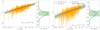 |
Fig. A.1. DM-only true mass-observed richness relation for the clusters at redshift z = 0.22. The richnesses have been measured using the two corresponding hydro runs – GadgetX and GIZMO-SIMBA – and considering the three projections per cluster. The solid green lines show the linear regression model results, with the coloured corresponding shaded region indicating the 1 σ uncertainty on the intercept and slope parameters. The dotted black and magenta long-dashed lines report to the model for the true hydro and weak lensing masses, as discussed in the main text. The corresponding right sub-panels display the PDF of the observed richnesses with respect to the best-fit linear model, with the shaded regions marking the corresponding σlog λobs. |
In Tab. A.1, we summarise the evolution of the intercept A, the slope B and the derived scatter σlog λobs as a function of redshift computed for the four considered stellar mass cuts, in the DM-only true mass-observed richness relation.
True DM-only mass-richness relation parameters.
All Tables
All Figures
|
Fig. 1. Simulated convergence maps of a cluster lens, namely with ID = 4, at zl = 0.22 and considering zs = 3, obtained by collapsing the total mass along the z-projection. The left and the central panels show the results using two different hydro-solvers GadgetX and GIZMO-SIMBA, respectively. In the right panel, we display the convergence map of the same cluster projection simulated using only collisionless dark matter particles, DM-only run. The assumed field of view is 5 Mpc by side, collapsing ±5 Mpc matter along the line-of-sight. |
| In the text | |
|
Fig. 2. Excess surface mass density profile of the projections displayed in Fig. 1. The colours used for the data points, blue, red and green, correspond to the GadgetX, GIZMO-SIMBA and DM-only run, respectively. The bottom panel displays the relative difference with respect to the DM-only case. The best-fit models are shown using solid curves, coloured according to each considered case. |
| In the text | |
|
Fig. 3. Posterior distributions of derived weak-lensing mass and concentration from the three weak-lensing simulations of the cluster of Fig. 1 and Fig. 2. The dashed lines indicate the three-dimensional mass and concentration for the DM-only cluster run. |
| In the text | |
|
Fig. 4. Average weak-lensing mass biases as a function of the corresponding three-dimensional masses. On the left, the weak lensing masses are relative to their respective total mass; on the right, they are always related to the total mass of the DM-only runs. The top and bottom sub-panels show the mean relative uncertainties and the relative differences with to the DM-only case as a function of considered three-dimensional reference mass, respectively. The right panels display the distribution of the weak-lensing mass biases over all cluster masses. The dark and light yellow bands show the 10% and 20% differences, respectively. |
| In the text | |
|
Fig. 5. Average weak-lensing mass biases as a function of redshift. Data points with error bars, colour-coded according to their DM-only corresponding mass, show the dark matter-only run results. Blue and red lines refer to the GadgetX and GIZMO-SIMBA hydro simulation cases, respectively. Dotted and solid lines show the bias in relation to the hydro mass and the DM-only mass, respectively. |
| In the text | |
|
Fig. 6. Halo and subhalo distribution in the projection x-y considering a field of view of 10 Mpc on a side and ±5 Mpc along the line of sight, ΔH = 10 Mpc, for the GadgetX cluster run. Black circles show the location of the centre of all subhaloes within the halo radius R200, red triangles are all haloes which, in projection, fall within the halo radius, and magenta crosses are all haloes that, in projection, lie in a ring between 2 and 3.5 R200, which we term outer haloes. The blue map is the corresponding region where we simulate the weak-lensing cluster signal. |
| In the text | |
|
Fig. 7. Weak-lensing mass-observed richness relation measured for the clusters at redshift z = 0.22 run with GadgetX. The different panels consider different minimum stellar mass cuts Mstar, min, from 1010 to 1010.75 h−1 M⊙. The weak-lensing masses Mwl are rescaled with respect to the pivot value Mp = 3 × 10¹⁴ h−1 M⊙. The blue points with the corresponding error bars show the results for the observed richness calculated as in Eq. (14) and the derived weak-lensing mass from the tangential shear profile. For the magenta triangles, the mass is not Mwl, but M200; correspondingly we show the number λint of galaxies within R200. The green circles show the results when using Mwl and the number of subhaloes in a sphere with radius R200. The solid blue line displays the results of our fit performed using MCMC on the blue data points, and in cyan, the 1σ uncertainty. The orange dash-dotted line is the best fit of the inverse relation; see Eq. (18). Black dotted lines display the model presented in this work, WLOR relation as in Eq. (15) considering the values reported in Table 1. |
| In the text | |
|
Fig. 8. Weak-lensing mass-observed richness relation measured for the clusters at redshift z = 0.22 run with both hydrocodes GadgetX in blue and GIZMO-SIMBA in red, respectively. The blue points are thus the same from Figure 7. The solid lines show the linear regression model results, with the shaded region indicating the 1σ uncertainty on the intercept and slope parameters. In each sub-figure – where we consider two different stellar mass cuts when computing λobs, the right sub-panel shows the PDF of the scatter of the observed richness (using a Gaussian KDE) with respect to the best-fit linear regression model; the shaded bands mark the corresponding 1σ deviation: σlog λ. |
| In the text | |
|
Fig. 9. Intercept A, slope B, and scatter σlog λobs at a fixed weak-lensing cluster mass as a function of redshift. Blue and red curves refer to the two hydro simulations: GadgetX and GIZMO-SIMBA, respectively. In all panels, the results referring to a given stellar mass cuts are reported with different line styles. The black curves show the best-fit models as a function of redshift, combining both hydro run results at a fixed stellar mass cut. The best-fit values are reported in Table 1. |
| In the text | |
|
Fig. 10. Observed richness-weak-lensing mass relation comparison with different literature results. We compute our model considering an observed richness with a minimum stellar mass of Mstar, min = 1010 h−1 M⊙ and the parameters have been calculated at z = 0.35. All redMaPPer (Rykoff et al. 2014) richness definitions have been rescaled to DES-Y1 by McClintock et al. (2019) (see their Table 5). The two dotted lines referring to KiDS-DR3 clusters from Lesci et al. (2022a) and Bellagamba et al. (2019) have been computed with the AMICO cluster finder algorithm (Maturi et al. 2019). |
| In the text | |
|
Fig. 11. True mass-observed richness relation for the clusters at redshift z = 0.22 as measured in both hydro-runs. The solid lines show the linear regression model results, with the shaded region indicating the 1σ uncertainty on the intercept and slope parameters. In each sub-figure, the right sub-panel shows the probability distribution function of the λobs with respect to the corresponding best-fit linear model, with the shaded regions marking the corresponding scatter σlog λobs. The dotted black lines exhibit the model for the richness weak-lensing mass relation, as described in the last section. |
| In the text | |
|
Fig. A.1. DM-only true mass-observed richness relation for the clusters at redshift z = 0.22. The richnesses have been measured using the two corresponding hydro runs – GadgetX and GIZMO-SIMBA – and considering the three projections per cluster. The solid green lines show the linear regression model results, with the coloured corresponding shaded region indicating the 1 σ uncertainty on the intercept and slope parameters. The dotted black and magenta long-dashed lines report to the model for the true hydro and weak lensing masses, as discussed in the main text. The corresponding right sub-panels display the PDF of the observed richnesses with respect to the best-fit linear model, with the shaded regions marking the corresponding σlog λobs. |
| In the text | |
Current usage metrics show cumulative count of Article Views (full-text article views including HTML views, PDF and ePub downloads, according to the available data) and Abstracts Views on Vision4Press platform.
Data correspond to usage on the plateform after 2015. The current usage metrics is available 48-96 hours after online publication and is updated daily on week days.
Initial download of the metrics may take a while.