| Issue |
A&A
Volume 697, May 2025
|
|
|---|---|---|
| Article Number | A33 | |
| Number of page(s) | 22 | |
| Section | Cosmology (including clusters of galaxies) | |
| DOI | https://doi.org/10.1051/0004-6361/202553914 | |
| Published online | 01 May 2025 | |
The impact of baryons on the sparsity of simulated galaxy clusters from THE THREE HUNDRED Project
Astrophysical and cosmological implications
1
LUX, Observatoire de Paris, Université PSL, Sorbonne Université, CNRS, 92190 Meudon, France
2
Sorbonne Université, CNRS, UMR 7095, Institut d’Astrophysique de Paris, 98 bis bd Arago, 75014 Paris, France
3
Donostia International Physics Center (DIPC), Paseo Manuel de Lardizabal, 4, 20018 Donostia-San Sebastián, Gipuzkoa, Spain
4
INAF, Osservatorio di Astrofisica e Scienza dello Spazio, via Piero Gobetti 93/3, I-40129 Bologna, Italy
5
INFN, Sezione di Bologna, Viale Berti Pichat 6/2, I-40127 Bologna, Italy
6
Dipartimento di Fisica, Sapienza Università di Roma, Piazzale Aldo Moro 5, I-00185 Rome, Italy
7
INAF-Osservatorio Astronomico di Trieste, Via Tiepolo 11, I-34131 Trieste, Italy
8
IFPU-Institute for Fundamental Physics of the Universe, via Beirut 2, 34151 Trieste, Italy
9
Department of Physics, University of Michigan, 450 Church St, Ann Arbor, MI 48109, USA
10
Departamento de Física Teórica, Módulo 15, Facultad de Ciencias, Universidad Autónoma de Madrid, 28049 Madrid, Spain
11
Centro de Investigación Avanzada en Física Fundamental (CIAFF), Facultad de Ciencias, Universidad Autónoma de Madrid, 28049 Madrid, Spain
12
INAF – Istituto di Astrofisica e Planetologia Spaziali, via Fosso del Cavaliere 100, I-00133 Rome, Italy
13
Université Paris Cité, F-75006 Paris, France
⋆ Corresponding authors: This email address is being protected from spambots. You need JavaScript enabled to view it.
; This email address is being protected from spambots. You need JavaScript enabled to view it.
Received:
27
January
2025
Accepted:
19
March
2025
Abstract
Context. Measurements of the sparsity of galaxy clusters can be used to probe the cosmological information encoded in the host dark matter halo profile, and infer constraints on the cosmological model parameters. Key to the success of these analyses is the control of potential sources of systematic uncertainties. As an example, the presence of baryons can alter the cluster sparsity with respect to predictions from N-body simulations. Similarly, a radial-dependent mass bias, as in the case of cluster masses inferred under the hydrostatic equilibrium (HE) hypothesis, can affect sparsity estimates.
Aims. First, we examined the imprint of baryonic processes on the sparsity statistics. Then, we investigated the relation between cluster sparsities and the gas mass fraction. Finally, we performed a study of the impact of HE mass bias on sparsity measurements and the implication on cosmological parameter inference analyses.
Methods. We used catalogues of simulated galaxy clusters from THE THREE HUNDRED project and ran a comparative analysis of the sparsity of clusters from hydrodynamical N-body simulations implementing different feedback model scenarios.
Results. Sparsities that probe the mass profile across a large radial range are affected by the presence of baryons in a way that is particularly sensitive to astrophysical feedback, whereas those exclusively probing external cluster regions are less affected. In the former case, we find the sparsities to be moderately correlated with measurements of the gas fraction in the inner cluster regions. We inferred constraints on S8 using synthetic average sparsity measurements generated to evaluate the impact of baryons, selection effects and HE bias. In the case of multiple sparsities (s200, 500, s200, 2500, and s500, 2500), these lead to highly biased results. Hence, we calibrated linear bias models that enabled us to correct for these effects and recover unbiased constraints that are significantly tighter than those inferred from the analysis of s200, 500 only.
Key words: galaxies: clusters: general / galaxies: clusters: intracluster medium / large-scale structure of Universe
© The Authors 2025
 Open Access article, published by EDP Sciences, under the terms of the Creative Commons Attribution License (https://creativecommons.org/licenses/by/4.0), which permits unrestricted use, distribution, and reproduction in any medium, provided the original work is properly cited.
This article is published in open access under the Subscribe to Open model. This email address is being protected from spambots. You need JavaScript enabled to view it. to support open access publication.
1. Introduction
There is a widespread consensus that observations of galaxy clusters can provide constraints on cosmological model parameters through a variety of observable properties (see e.g. Allen et al. 2011; Kravtsov & Borgani 2012). The availability of large homogeneous galaxy cluster samples has enabled, in recent years, the realisation of cosmological data analyses through measurements of the cluster abundance (see e.g. Planck Collaboration XX 2014; Planck Collaboration XXIV 2016; Pacaud et al. 2018; Bocquet et al. 2019; Lesci et al. 2022; To et al. 2021), spatial clustering (Planck Collaboration XXI 2014; Marulli et al. 2021), as well as estimates of the cluster gas mass fraction (see e.g. Ettori et al. 2009; Mantz et al. 2014, 2022; Wicker et al. 2023). Cosmological information is also encoded in the spatial distribution of mass within clusters. This is because galaxy clusters are hosted in massive dark matter (DM) haloes, which are the result of the hierarchical bottom-up gravitational assembly process of cosmic structure formation (see e.g. Wechsler et al. 2002; Ludlow et al. 2013; Wang et al. 2020; Richardson & Corasaniti 2022). Such a process depends on the global properties of the universe, such as the cosmic matter density, the state of cosmic expansion, and the amplitude of initial matter density fluctuations, thus leaving a cosmological imprint on the radial mass profile of clusters.
The possibility of testing cosmology through measurements of the distribution of mass within clusters has primarily been investigated in the context of a parametric description of the host DM halo density profile. This is motivated by the analysis of N-body simulations that have shown that the spherically averaged halo density profile is well-fitted by a two-parameter formula, the Navarro–Frenk–White (NFW) profile (Navarro et al. 1997), which is fully specified by the halo mass M and the concentration parameter c.
Numerical studies have shown that the concentration relates to the halo formation history and the halo dynamical state (see e.g. Wechsler et al. 2002; Neto et al. 2007; Zhao et al. 2009; Ludlow et al. 2012, 2013; Lee et al. 2017; Rey et al. 2019). However, due to the stochastic nature of the gravitational collapse that drives the halo assembly process, the concentration behaves as a random variate characterised by a large scatter and a median that varies as a function of halo mass (see e.g. Bullock et al. 2001; Zhao et al. 2003; Macciò et al. 2007; Prada et al. 2012; Ishiyama et al. 2021). Quite importantly, the amplitude of such a relation has been found to depend on the underlying cosmological model (see e.g. Bullock et al. 2001; Dolag et al. 2004; Zhao et al. 2009; Giocoli et al. 2012), thus opening the possibility to infer cosmological parameter constraints from measurements of the concentration-mass relation. Nevertheless, this has proven to be challenging (see e.g. Ettori et al. 2010), since systematic uncertainties, such as selection effects (Sereno et al. 2015) and the astrophysical process altering the matter distribution in galaxy clusters (see e.g. Mead et al. 2010; King & Mead 2011; Rasia et al. 2013), can significantly impact the determination of the concentration parameter of galaxy clusters.
Alternatively, Balmès et al. (2014) have proposed a non-parametric approach based on measurements of ratios of spherical halo masses estimated at radii enclosing different overdensities. These ratios, dubbed sparsities, probe the level of sparseness of the halo mass distribution, while retaining cosmological information encoded in the halo mass profile (Balmès et al. 2014; Corasaniti et al. 2020). In particular, this can be retrieved through measurements of the average sparsity of a sample of clusters at different redshifts (Corasaniti et al. 2018; Richardson & Corasaniti 2023). Furthermore, the combination of measurements of average sparsities for multiple overdensity pairs can provide stronger constraints by extracting the cosmological signal imprinted across the entire halo mass profile, beyond what is captured by the NFW’s concentration (Corasaniti et al. 2022). Recently, Richardson & Corasaniti (2023) have also shown that constraints can also be obtained from individual cluster sparsity measurements, rather than ensemble average estimates, provided the availability of predictions of the sparsity probability distribution function from N-body simulations.
Cosmological parameter constraints have been inferred from measurements of the average sparsity of X-ray (Corasaniti et al. 2018) and weak gravitational lensing (Corasaniti et al. 2021) mass estimates of cluster samples. These studies have shown that current sparsity estimates are primarily limited by the large statistical uncertainties affecting the mass measurements of observed galaxy clusters. Nonetheless, in upcoming years, these are expected to improve thanks to a new generation of cluster survey programmes such as the CHEX-MATE project1 (CHEX-MATE Collaboration 2021) or the Euclid mission (see e.g. Sartoris et al. 2016; Euclid Collaboration 2019). Hence, in preparation of the future cosmological analyses, it is of primary importance to study potential sources of systematic errors that can affect the cosmological model parameter inference. For instance, the presence of baryons may alter the predictions of the sparsity with respect to that inferred from DM-only simulations. Similarly, a radial- (aperture-) dependent mass bias can affect the determination of the cluster sparsity and induce a sparsity bias. As an example, deviations from the hydrostatic equilibrium (HE) hypothesis may result in a radial-dependent bias of the cluster masses obtained from the analysis of X-ray and Sunyaev-Zel’dovich (SZ) observations of galaxy clusters, thus leading to biased sparsity estimates. Assessing these systematics requires us to investigate the statistical properties of sparsity using hydrodynamical simulations. A first analysis of this type has been presented in Duffy et al. (2010), where the authors used hydrodynamical simulations to investigated the modifications induced by the baryons on the density profile of massive galaxies and clusters as traced by the ratio of radii enclosing two different overdensities. However, this early study never considered the possibility that these non-parametric proxies can be used to probe cosmology, as shown in the subsequent series of articles dedicated to the sparsity, or to capture the imprint of astrophysical processes that occurs in the inner regions of clusters, as we subsequently show in this work.
Here, we perform a thorough analysis of the sparsity statistics using the simulated cluster catalogues from THE THREE HUNDRED project (Cui et al. 2018), hereafter The300. Our goal is twofold. On the one hand, we aim to study the extent to which baryons (gas and stars) alter the mass profile of clusters, as probed by sparsity. To this purpose, we evaluate the deviation of sparsities of clusters from hydrodynamical simulations against those estimated from DM-only simulations. This enables us to evaluate the sensitivity of different sparsities to the effect of astrophysical processes parameterised by the sub-grid models implemented in The300. On the other hand, we investigate the effect of mass and selection bias on the cosmological parameter inference of a synthetic sample of sparsity data generated using the HE mass estimates obtained by Gianfagna et al. (2023) from the analysis of The300.
The article is organised as follows: in Section 2 we introduce the sparsity statistics and describe the simulation dataset used in our analysis. In Section 3, we present the results of numerical analyses devoted to the assessment of the statistical representativeness of the sparsity samples, the evaluation of the impact of baryons on the halo sparsities and the role of baryonic feedback models. In Section 4, we discuss the astrophysical implications of such effects, while in Section 5 we present the analysis of the impact of the HE mass bias on the cluster sparsities. In Section 6, we discuss the cosmological implications of the HE mass bias and selection effects and evaluate their effects on cosmological parameter inference analyses. Finally, in Section 7 we present our conclusions.
2. Methodology
2.1. Dark matter halo sparsity
Dark matter halo sparsity is defined as follows (Balmès et al. 2014):
 (1)
(1)
where MΔ1 and MΔ2 are the masses enclosed in spheres of radii rΔ1 and rΔ2, that contain the overdensity Δ1 and Δ2 respectively, where Δ1 < Δ2. Notice that the sparsity can be written as a fractional mass estimate, sΔ1, Δ2 = ΔM12/MΔ2 + 1, where ΔM12 = MΔ1 − MΔ2 is the mass enclosed within the radial shell comprised between the outer radius rΔ1 and the inner radius rΔ2. Hence, depending on the choice of Δ1 and Δ2 the sparsity provides a proxy of the fractional halo mass profile in different halo regions2. Hereafter, we will always refer to masses at overdensities given in units of the critical density.
2.2. Numerical simulation dataset
Here, we describe the numerical simulations we have used in our analyses. Specifically, we have used the simulations realised in the context of THE THREE HUNDRED project collaboration3 to investigate the impact of baryons on the sparsity of halos relies. We have also used the halo catalogues from the UCHUU simulation suite (Ishiyama et al. 2021) to calibrate the halo mass function used in the cosmological parameter inference analyses and the evaluation of selection bias effects.
2.2.1. The Three Hundred
We use catalogues of simulated galaxy clusters from The300 (Cui et al. 2018). These have been generated from zoom simulations of 324 spherical regions of 15 h−1 Mpc radius centred on the most massive haloes of the MultiDark-Planck2 (MDPL2) simulation (Klypin et al. 2016) detected at redshift z = 0 using the ROCKSTAR4 halo finder (Behroozi et al. 2013). These regions have been re-simulated assuming purely gravitational physics (DM-only) and including baryon hydrodynamics with different sub-grid models. Cluster catalogues were then generated using the AHF5 (Knollmann & Knebe 2009) halo finder.
The simulations assume a flat ΛCDM model with parameters set to the values inferred from the Planck data analysis (Planck Collaboration XIII 2016): total matter density Ωm = 0.307, baryon density Ωb = 0.048, reduced Hubble constant h = 0.678, amplitude of linear matter density fluctuations on 8 h−1 Mpc scale σ8 = 0.823, and scalar spectral index ns = 0.96.
The GIZMO-SIMBA zoom simulations (see Cui et al. 2022, for more details) have been realised with the GIZMO code (Hopkins 2015) implementing the sub-grid model from the SIMBA simulation (Davé et al. 2019). The GADGET-MUSIC simulations were carried out with the GADGET-3 Tree-PM gravity solver (an updated version of GADGET-2 code by Springel 2005) implementing a classic entropy-conserving formulation smoothed-particle hydrodynamics (SPH) scheme with the baryonic physics described in Sembolini et al. (2013), while the GADGET-X simulations were realised using an improved version of the SPH scheme by Beck et al. (2016) with the baryon physics models discussed in Rasia et al. (2015). Notice that both GIZMO-SIMBA and GADGET-X simulations include AGN feedback, though with different model characteristics, while the GADGET-MUSIC runs do not. Because of this the simulated clusters from the GIZMO-SIMBA and GADGET-X catalogues have properties that are better in agreement with observations (see Cui et al. 2018, 2022).
In the analysis presented here, we consider the most massive cluster of each of the 324 re-simulated regions of the GADGET-X, GADGET-MUSIC, GIZMO-SIMBA, and DM-only simulations, for which we compute the sparsity for several pairs of overdensities. In particular, we compute the mass MΔ at Δ = 200, 500, 1000, 1500, 2000 and 2500 for each of the clusters in the numerical catalogues. Then, we estimate the sparsity for different combination of overdensities as defined by Eq. (1). We note that in the case of the catalogues from the hydrodynamical simulations, the mass MΔ is the total cluster mass, that is the sum of the mass in the dark matter, gas mass and stellar component within RΔ.
In order to distinguish the effect of the baryons from that of the dynamical state of clusters, we perform a statistical analysis of the sparsity on a subsample of relaxed objects from each of the numerical catalogues listed above. More specifically, we select systems that object-by-object are characterised by the virial energy ratio η, the centre-of-mass offset Δr and the fraction of mass in sub-haloes fs (all evaluated within R200) within the following bounds: 0.85 < η < 1.15, Δr < 0.04 and fs < 0.1 both for the hydrodynamical case and their DM-only counterpart. Notice that the bounds adopted here are identical to those assumed in Cui et al. (2018), although our selection is more restrictive since for each cluster in the relaxed subsample the above conditions need to be fulfilled simultaneously in both the hydrodynamical and DM-only simulations. It is worth mentioning that such a characterisation results in a binary selection of clusters. This differs from the approach adopted in Haggar et al. (2020), where the authors introduce a parameter, χDS, which links the values of η, Δr and fs, with the intent of obtaining a continuous measure of the dynamical state. Furthermore, as pointed out in De Luca et al. (2021) these indicators may vary depending on the overdensity at which they are evaluated. Quite remarkably, their analysis of The300 shows that the fraction of relaxed clusters selected with criteria adopted in Cui et al. (2018) remains unaltered whether the dynamical indicators are evaluated at R200 or R500. This is due the aperture dependence of η and results in more stringent criterion. Indeed, our selection is more restrictive than that assumed in Cui et al. (2018), which enables us to more easily distinguish the impact of baryons on the halo sparsity with respect to that of the dynamical state.
Finally, in order to assess the impact of the HE mass bias on sparsity measurements, we use the three-dimensional HE mass estimates from the analysis of the GADGET-X clusters presented in Gianfagna et al. (2023). These have been estimated for the most massive cluster of each of the zoomed regions of the GADGET-X simulation that contain no low-resolution particles within the virial radius of the cluster.
2.2.2. UCHUU
We use the halo catalogues from the UCHUU N-body simulation suite (Ishiyama et al. 2021) of (2 h−1 Gpc)3 volume with 128003 particles realised with the code GreeM (Ishiyama et al. 2009, 2012). As in the case of The300, the simulation assume a flat ΛCDM model with parameters set to the Planck-CMB 2015 analysis (Planck Collaboration XIII 2016): Ωm = 0.3089, Ωb = 0.0486, h = 0.6774, ns = 0.9667, and σ8 = 0.8159. Notice that these differ at sub-percent level from those assumed in the The300.
Haloes have been detected with the ROCKSTAR halo finder (Behroozi et al. 2013) and spherical masses at different overdensities have been computed for all detected halos in 24 redshift snapshots in the range 0 ≤ z ≤ 2.
3. Numerical data analyses
3.1. Statistical representativeness
The sample of simulated clusters from The300 project, corresponds to the 324 most massive haloes detected in the MDPL2 simulation at z = 0 and followed throughout their evolution. Hence, the sample is mass-selected and volume-limited only for z = 0, while the selection is unclear at higher redshifts. Given that we are interested in evaluating the impact of baryons on the sparsity statistics, it is worth assessing the representativeness of the estimated sparsities. Even though we can perform such a test only for the DM-only catalogue, this remains a useful check. For conciseness, we limit ourselves to the catalogues at z = 0.0, 0.5 and 1.0, for which we can confront the distribution of sparsities inferred using the DM-only halo catalogue of The300 (The300/DM-only) against those obtained from the MDPL2 haloes with masses larger than the minimum halo mass of the The300/DM-only catalogue, that is M200 ≳ 5 ⋅ 1014 h−1 M⊙ at z = 0.0, ≳1014 h−1 M⊙ at z = 0.5 and ≳6 ⋅ 1013 h−1 M⊙ at z = 1.0. This selection results in a reference MDPL2 halo subsample of Nhalo = 612 haloes at z = 0.0, Nhalo = 8368 at z = 0.5 and Nhalo = 8162 at z = 1.0.
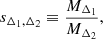
As the publicly available MDPL2 halo catalogues provide estimates of the halo masses at overdensity Δ = 200, 500 and 2500, we only consider the following set of sparsities: s200, 500, s200, 2500 and s500, 2500. In Fig. 1, we plot the normalised histograms of s200, 500 (left panel), s200, 2500 (central panel) and s500, 2500 (right panel) for the MDPL2 subsample (blue bars) and The300/DM-only catalogues (goldenrod filled bars) at z = 0.000 (top panels), 0.523 (middle panels) and 1.031 (bottom panels) respectively. The vertical lines in the panels correspond to the median values of the sparsity distribution for the MDPL2 subsample (dark blue dotted line) and the The300/DM-only sample (goldenrod solid line). We can see that independently of the redshift both samples span the same range of sparsity values. Moreover, we find that the distribution of sparsities are very similar to one another, with the median sparsities of the two samples having nearly identical values. This is confirmed by the estimation of the Kullback–Leibler (KL) divergence (Kullback & Leibler 1951). In particular, by assuming the histogram of the MDPL2 subsample to be the target distribution, we find the KL divergence of The300/DM-only sample to be 𝒟KL = 0.17 in the case of s200, 500, 𝒟KL = 0.04 for s200, 2500 and 𝒟KL = 0.08 for s500, 2500 at z = 0. Such an agreement might be expected given that The300 sample is mass-selected at z = 0. However, we can see that this remains valid also at higher redshifts. In particular, at z = 0.5 we have 𝒟KL = 0.03 in the case of s200, 500, 𝒟KL = 0.08 for s200, 2500 and 𝒟KL = 0.09 for s500, 2500, and similar values at z = 1. Hence, despite the difference in sample size and the fact that the MDPL2 haloes were detected using the ROCKSTAR halo finder, rather than AHF, the distributions of sparsities are compatible with one another. We can conclude that the sparsities from the The300/DM-only are representative of the population of very massive haloes from the larger volume MDPL2 simulation. Nonetheless, this does not ensure that the sparsities of the clusters from the zoom hydrodynamical simulations are also representative of the statistics of a large volume sample. Conservatively, it only guarantees that the distribution of sparsities of our reference DM-only sample is not affected by volume effects.
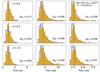 |
Fig. 1. Normalised histograms of the sparsity s200, 500 (left panels), s200, 2500 (central panels), and s500, 2500 (right panels) obtained from the analysis of the MDPL2 sub-sample (dark blue bars) and The300/DM-only catalogue (goldenrod filled bars) at z = 0.0 (top panels), 0.5 (middle panels), and 1.0 (bottom panels), where the MDPL2 sub-sample consists of haloes with a mass larger than the minimum mass of the DM-only catalogue at the redshift considered. The vertical lines in each panel correspond to the median sparsities for the MDPL2 sub-sample (dark blue dotted line) and the The300/DM-only sample (goldenrod solid line). |
A subtle point we would like to stress here is the fact that even if such representativeness may extend to the hydrodynamical cluster samples, by no means it entails that the selected clusters are representative of a cosmological selection. This is because the clusters considered here are not randomly drawn from the halo mass function distribution, rather that each of them is drawn from an extreme value distribution of the first to 324th order most massive halo. This inevitably results in selection effects that need to be accounted when evaluating the cosmological information encoded in the sparsity from The300. As we will see in Sec. 6, this is particularly important when assessing the impact of the HE mass bias on the cosmological parameter constraints inferred from sparsities measurements obtained using HE mass estimates from a subsample of the most massive clusters from the GADGET-X simulations.
3.2. The impact of baryons on the cluster sparsity
Let us now focus on how baryons alter the mass profiles of simulated clusters as traced by sparsity. We can infer a first qualitative insight by comparing the sparsity of the haloes in the DM-only simulation against that of the corresponding clusters in the hydro simulations. In principle, we could choose the sparsity between any pair of overdensities, provided that Δ1 < Δ2. Nonetheless, it is convenient to use overdensity values that are commonly adopted in observational studies. In particular, let us consider the sparsities s200, 500, s500, 1000 and s1000, 2500, which respectively probe the fractional mass profile in the external, intermediate and inner halo regions.
In Fig. 2 we plot the different sparsities in the case of the full sample of 324 clusters (blue squares) for the GIZMO-SIMBA (top panels), and GADGET-X (central panels) and GADGET-MUSIC(bottom panels) catalogues at z = 0 against the sparsities of their DM-only counterparts. We also plot the comparison for the relaxed systems (yellow triangles) consisting of 62 clusters from the GIZMO-SIMBA subsample, 68 from GADGET-X and 64 from GADGET-MUSIC. The diagonal line corresponds to the ideal case with the cluster sparsities being equal to that of the DM-only haloes, while the shaded areas corresponds to 10% (yellow band) and 50% (light-blue band) deviations respectively. The size of the data points in the plots is set to be proportional to the DM-only mass, M200.
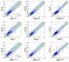 |
Fig. 2. DM-only versus hydro-simulation-estimated sparsities s200, 500 (left panels), s500, 1000 (central panels) and s1000, 2500 (right panels) for the clusters in the GIZMO-SIMBA (top panels), GADGET-X (central panels), and GADGET-MUSIC (bottom panels) catalogues at z = 0, respectively. The blue squares represent clusters from the full samples, while the yellow triangles corresponds to the relaxed systems as defined in Sec. 2.2. The size of the data points is proportional to mass M200 of each cluster from the DM-only simulation. The diagonal line represents the ideal case with no bias, while the shaded areas correspond to 10% (yellow band) and 50% (light-blue band) deviation respectively. |
First of all, we can see that in all the cases the sparsities are distributed along the diagonal line. The bulk of the clusters lies well within 50% of the ideal case, and within ∼10% in the case of relaxed systems. We can also notice that in the case of the full cluster sample, the scatter around the diagonal line increases for greater values of the cluster sparsity. This can be the results of multiple factors due to the interplay between the dynamical status of the clusters (Richardson & Corasaniti 2022), the delay in the assembly of substructures between DM-only and hydrodynamical simulations (see Sembolini et al. 2013) and the survival rate of substructure due to baryon physics. As far as the dependence on the halo mass is concerned, we do not find any particular trend and we refer the reader to Appendix A for a more detailed analysis.
3.2.1. Cluster sparsity: DM-only versus hydrodynamical simulations
We use the spherical masses at different overdensities computed for each of the clusters in the hydrodynamical and DM-only catalogues to estimate the sparsities sΔ1, Δ as a function of Δ for Δ > Δ1 with Δ1 = 200, 500 and 1000. Then, we compare the sparsity of each clusters in the hydrodynamical catalogue to that of its DM-only counterpart. More specifically, we compute for the i-th cluster the relative difference:
 (3)
(3)
We find the distribution of values of Eq. (3) to be well approximated by a Gaussian distribution. Hence, as summary statistics, we adopt the mean ⟨Δs/s⟩ and the standard deviation σΔs/s estimated for each cluster sample. These are shown in Fig. 3 for the GIZMO-SIMBA clusters, in Fig. 4 for the GADGET-X clusters and in Fig. 5 for the GADGET-MUSIC clusters. The left (right) panels show the summary statistics for the catalogues at z = 0 (z = 1).
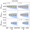 |
Fig. 3. Sparsity relative difference Δs/s |200, Δ (top panels), Δs/s |500, Δ (central panels), and Δs/s |1000, Δ (bottom panels) as function of Δ for the GIZMO-SIMBA clusters in the catalogues at z = 0 (left panels) and 1 (right panels). The blue squares (yellow triangles) represent the average for the full (relaxed) cluster sample, while the shaded areas correspond to the standard deviation. The black dashed lines in the plots mark the 5% differences respectively, while the solid blue (yellow) lines correspond to the linear regression of the average values. |
Firstly, we may notice that in all the cases the absolute value of the average sparsity relative difference ⟨Δs/s⟩Δ1, Δ tends to linearly increase as function of Δ, though the sign and amplitude of the variation depend on the simulated cluster sample. This is due to the different sub-grid models implemented in the different hydro simulations. In particular, we find that on average the GIZMO-SIMBA clusters have greater sparsities than their DM-only counterparts (⟨Δs/s⟩Δ1, Δ < 0), while GADGET-MUSIC clusters exhibit smaller ones (⟨Δs/s⟩Δ1, Δ > 0). The GADGET-X clusters represents an intermediary case, with smaller relative difference.
Secondly, we may notice that the standard deviation of the sparsity relative difference also increases as function of Δ, though the level of scatter is smaller for the sample of relaxed clusters. As already mentioned in Sec. 3.2, this indicative of the fact that deviations from the dynamical equilibrium largely contribute to the difference between the sparsity estimated from DM-only simulations and hydrodynamical one.
Hereafter, we provide a more quantitative description of the observed trends. In the case of the GIZMO-SIMBA clusters at z = 0, we find for the full sample that −1%≲⟨Δs/s⟩200, Δ ≲ −7% for 500 ≤ Δ ≤ 2500, −3%≲⟨Δs/s⟩500, Δ ≲ −8% for 1000 ≤ Δ ≤ 2500, and −1%≲Δs/s⟩1000, Δ ≲ −5% for 1500 ≤ Δ ≤ 2000. In the case of the scatter, we find 7%≲σΔs/s|200, Δ ≲ 17%, 9%≲σΔs/s|500, Δ ≲ 21%, and 7%≲σΔs/s|1000, Δ ≲ 15%. A similar trend occurs at z = 1. Notice that in the case of the relaxed clusters, we find similar values for the average relative difference both at z = 0 and 1, while the scatter results nearly a factor of two smaller than that found from the full sample.
In the case of GADGET-X clusters at z = 0, we find for the full sample that ⟨Δs/s⟩200, Δ remains approximately constant as function of Δ with a value ∼2%. On the other hand, we find the average relative difference to be at sub-percent level in the case of ⟨Δs/s⟩500, Δ and ⟨Δs/s⟩1000, Δ. We obtain similar values in the case of the relaxed systems. As far as the scatter is concerned, it varies between ∼7% and ∼18% for the different sparsity configurations. At z = 1 we observe a similar trend. Also in this case, the relaxed clusters exhibit similar values of the average relative difference of the sparsity configurations compared to the full case with nearly a factor of two smaller scatter.
Finally, in the case of the GADGET-MUSIC clusters at z = 0, we find for the full sample that ⟨Δs/s⟩200, Δ varies linearly between ∼2% and 8% for 500 ≤ Δ ≤ 2500, while ⟨Δs/s⟩500, Δ varies in the range 2 − 5% for 1000 ≤ Δ ≤ 2500 and ⟨Δs/s⟩1000, Δ varies between ∼1% and ∼4% in the rage 1500 ≤ Δ ≤ 2500. The standard deviation for the different sparsity configuration varies in the range ∼6% to ∼15%. In the case of the relaxed clusters we find similar values for the average relative difference, while the scatter is nearly a factor of two smaller. Similar trends occur for the z = 1 case.
3.2.2. Baryon feedback model dependence
The results of the previous analysis show that the presence of baryons alters the average sparsity with respect to the DM-only results. Such differences vary across the cluster mass profile in a way that depends on the sub-grid physics model implemented in the simulations. This suggests that certain sparsity combinations are more sensitive to the astrophysical processes that alter the mass distribution within clusters, while others are less affected and thus better suited for cosmological studies.
Here, we investigate this in more detail and we compute the average of the relative difference between the sparsities of the GADGET-X and GADGET-MUSIC clusters with respect to those from their GIZMO-SIMBA counterparts for different sparsity configurations, that is  . These are shown in Fig. 6 for the full and relaxed samples at z = 0 (top panels) and z = 1 (bottom panels) respectively, where the errorbars correspond to the standard deviation. First of all, we observe similar trends for both the full and relaxed cluster samples. Secondly, we notice that in the case of the full cluster samples the scatter is much larger than that obtained from the analysis of the relaxed systems. Hence, to better appreciate the effect of the sub-grid physics implemented in the hydrodynamical simulations, let us focus on the relaxed clusters.
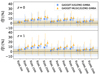 |
Fig. 6. Average and scatter of the relative difference of the sparsity of the GADGET-X (blue squares) and GADGET-MUSIC (yellow triangles) clusters with respect to that of their GIZMO-SIMBA counterparts for different sparsity configurations in the case of the full (filled markers) and relaxed (empty markers) samples at z = 0 (top panel) and 1 (bottom panel), respectively. The errorbars represent the standard deviations for each sparsity configuration, while the shaded areas correspond to 5% and 10% variation respectively. |
We can see that relative differences are minimal for sparsity configurations probing the mass profile between nearby mass shells. For instance, in the case of s200, 500, which probes the external regions of the cluster profile, we find differences consistent with 0 at 1σ for both GADGET-X and GADGET-MUSIC with respect to GIZMO-SIMBA clusters. Similarly, the differences in the case of s500, 1000 and s1000, 1500 never exceed the 5% level. In contrast, these increase for large overdensity separations probing the slope of the mass profile between inner and outer regions. As an example, s200, 2500 shows the largest differences of ∼8% (∼12%) for GADGET-X (GADGET-MUSIC) at z = 0 and ∼12% (∼18%) at z = 1.
The fact that at large overdensity separations the relaxed GIZMO-SIMBA clusters exhibit on average larger sparsities than their GADGET-X counterparts is a direct consequence of the different AGN feedback models implemented in the two simulations. More specifically, the GADGET-X simulation implements a thermal AGN feedback model, while the GIZMO-SIMBA simulations implement a kinetic one (see Cui et al. 2022, for more detail). The latter is more effective at displacing the gas from the centre of the cluster, which reduces the amount of total mass in the core region of the cluster relative to the external one, thus resulting in higher sparsities. Hence, it is not surprising that the differences are even greater in the case of the GADGET-MUSIC clusters, since the GADGET-MUSIC simulations do not implement any AGN feedback at all. In the latter case, the dark matter mass in the centre of the cluster undergoes adiabatic contraction due to the collapse of baryons (Gnedin et al. 2004; Teyssier et al. 2011; Martizzi et al. 2012). This leads to an increase of the total mass in the central region of the cluster relative to the outer one. Consequently, the GADGET-MUSIC clusters have smaller sparsities compared to those of the simulations that account for AGN feedback.
Overall, our analysis suggests that sparsities such as s200, 500 and s500, 1000 are less sensitive to the effects of baryon feedback models, as such they can be a better proxy of the cosmological signal encoded in the cluster mass profile. On the other hand, sparsities probing the slope of the mass distribution across a large radial interval (from external to inner regions), such as s200, 2500 and s500, 2500, are more sensitive to the effects of baryonic processes, potentially providing a proxy for cluster astrophysics.
4. Astrophysical implications
4.1. Sparsity vs gas fraction
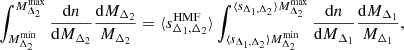
In the previous section, we have seen that the presence of the baryons alters the mass profile of clusters as probed by sparsity with respect to the predictions of DM-only simulations in a way that depends on the astrophysical feedback model assumptions. In principle, we may expect these processes to induce correlations between the mass distribution and astrophysical properties of the clusters. To address this point, we now investigate the relation between the mass profile of clusters as probed by the sparsity and the baryon content as traced by the gas fraction. We do not report the analysis of stellar mass fractions as we have found no correlations with the cluster sparsities.
In this analysis we only consider clusters from the GADGET-X and GIZMO-SIMBA simulations, which are better in agreement with observations. For each of the clusters in the samples, we estimate the gas fraction within RΔ, 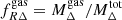 for Δ = 500 and 2500. We also consider the gas fraction in a shell comprised between R2500 and R500, defined as
  . For simplicity, we limit the analysis to sparsities s200, 500 and s500, 2500.
We evaluate the Pearson’ correlation coefficients,  , for the different sparsities and gas fraction configurations. These are shown in Fig. 7 as function of redshift for the GADGET-X (light blue markers) and GIZMO-SIMBA (yellow markers) in the case of the full (filled markers) and relaxed (empty markers) samples. The shaded areas corresponds to values of the Pearson coefficients indicative of correlations that are considered very weak (dark blue), weak (blue) and moderate (light-blue).
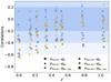 |
Fig. 7. Pearson’s correlation coefficients as function of redshift for the GIZMO-SIMBA (yellow markers) and GADGET-X (blue markers) clusters from the full (filled markers) and relaxed (empty markers) samples. The shaded areas (dark to light blue) correspond to “very weak”, “weak” and “moderate” correlations respectively. |
We remark that for a given sparsity configuration the correlation coefficients from the GIZMO-SIMBA clusters are systematically larger in absolute value than those from the GADGET-X ones. This is consistent with the fact that the AGN feedback model implemented in the GIZMO-SIMBA simulations is more efficient at displacing gas from the inner halo region than the thermal AGN model of the GADGET-X simulations, thus inducing a stronger correlation between the distribution of gas and total mass. Not surprisingly in the case of the GIZMO-SIMBA clusters, we find that at z = 0 s200, 500 and  , and s500, 2500 and
  are anti-correlated with a “strong” level of correlation (> 60%). At higher redshifts, the correlation among these variates diminishes, though remaining above the 20% level. In the case of the GADGET-X clusters, the most anti-correlated variables are s200, 500 and
  , and s500, 2500 and
  up to z ∼ 0.3 with a correlation coefficient varying in the range −0.6 ≲ ρs − fgas ≲ −0.4. At higher redshifts these variables become weakly correlated, while s500, 2500 and
  show a moderate correlation.
The relaxed clusters show correlations that are of slightly smaller amplitude than those inferred from the full cluster sample. Though, we should consider that for these samples, the estimation of the correlation coefficient is affected by a greater sample variance error, which is of order ∼20% to be compared with the ∼3 − 5% of the full cluster sample.
It is worth noticing that in all the cases s200, 500 and s500, 2500 appear to be weakly correlated with  . And given the fact that these sparsities are weakly correlated sparsities (see Fig. D.1 in Appendix D), their measurements can be combined together with gas fraction estimates within R500 to infer stronger cosmological constraints. In contrast, sparsities probing the slope of the cluster mass profile across a large radial range show a weak to a moderate correlation with gas fraction measurements that probe the gas distribution in inner cluster regions. The presence of such correlations can be tested through observations. As an example, in Fig. 8 we plot the values of s500, 2500 against the estimates of
  for the GIZMO-SIMBA and GADGET-X clusters at z = 0. We can see that the lower the differential gas fraction the higher the sparsity. Again, this is a direct consequence of the AGN feedback models adopted in the simulations. Indeed, we may remark that
  spans a lower range of values for the GIZMO-SIMBA clusters compared to the GADGET-X ones. This is because the kinetic AGN model is more efficient at displacing the gas in the inner halo region compared to the thermal one. This leads to lower values of the gas fraction, while at the same time it reduces the effect of the adiabatic contraction (Gnedin et al. 2004) and therefore of the total mass in the inner cluster regions, which results in higher sparsity.
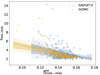 |
Fig. 8. s500, 2500 versus |

The trends shown in Fig. 8 can modelled in terms of a simple linear regression. We perform a Bayesian analysis to infer the slope and intercept for the GIZMO-SIMBA and GADGET-X clusters at different redshifts. In Table 1 we quote the average, standard deviation and best-fit values of the linear regression coefficients. At fixed redshifts the slopes from the two cluster samples are statistically consistent with one another, though the uncertainties are smaller for the GIZMO-SIMBA clusters consistently with their stronger level of correlation for the variables considered.
Bayesian linear regression of sparsity–gas fraction relation.
It would be interesting to perform such an analyses on a larger sample of simulated clusters, and eventually test such relations on observed cluster samples. We leave this to a future study.
4.2. Sparsity and gas fraction ratios
Given that mass ratios provide an estimate of the logarithmic slope of the radial mass profile, we want to test to which extent ratios of the gas mass fraction estimated at two different overdensities directly probe the cluster sparsity. To this purpose we compute the gas mass fraction within RΔ for Δ = 200, 500 and 2500 for each cluster in the GADGET-X and GIZMO-SIMBA samples. Then, we estimate the gas mass fraction ratios  and
and  . By definition rΔ1, Δ2gas ≡ sΔ1, Δ2gas/sΔ1, Δ2, hence if the mass gas fraction profile is constant then rΔ1, Δ2gas = 1 and sΔ1, Δ2gas exactly trace the cluster sparsity sΔ1, Δ2.
In Fig. 9 we plot the normalised histograms of  (top panels) and
  (bottom panels) for the GADGET-X (blue filled bars) and GIZMO-SIMBA (yellow filled bars) clusters at z = 0 (left panels), 0.5 (middle panels) and 1.0 (right panels) respectively. The histograms with empty bars correspond to the results from the analysis of the relaxed cluster samples. In Table 2, we quote the summary statistics for the different cases in terms of median, average and percentiles of the gas mass fraction ratios.
Summary statistics of  and
and  .
.
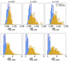 |
Fig. 9. Normalised histograms of the gas mass fraction ratios |


We can see that the distributions are skewed towards values larger than unity6. This is a direct consequence of the fact that the gas fraction decreases at lower cluster radii. This is a well known result both from numerical simulations (see e.g. Frenk et al. 1999; Rasia et al. 2004; Ettori et al. 2006; Planelles et al. 2013; Battaglia et al. 2013; Angelinelli et al. 2023, Rasia et al., in prep.) as well as observations of clusters (see e.g. Sadat et al. 2005; Pratt et al. 2010; Eckert et al. 2013; Mantz et al. 2016). In fact, even in non-radiative simulations, multiple astrophysical processes can deplete the gas mass from the inner cluster regions. Because of this, the gas mass fraction ratio is a biased tracer of the cluster sparsity, though the level of bias depends on the astrophysical processes that takes place in the intra-cluster medium. As an example, in the case of the GADGET-X clusters we have an average bias of ∼4% for s200, 500 in the redshift range 0 < z < 1, while in the case of the GIZMO-SIMBA sample this is of the order of ∼9 − 14%. In the case of s500, 2500, the bias between the gas mass fraction ratio and the sparsity is of the order of ≈20% for the GADGET-X and ≈60 − 70% for the GIZMO-SIMBA clusters respectively. We find results of the same order of magnitude in the case of the relaxed samples. The effect is larger on the GIZMO-SIMBA clusters than the GADGET-X ones, consistently with the fact that the AGN feedback model is more efficient at displacing the gas from the inner cluster regions in the former case than the latter. Indeed, we may consider that the difference between the GIZMO-SIMBA and GADGET-X distributions of the gas mass fraction ratios are a distinct signature of the feedback scenario implemented in the simulations, possibly providing a test against measurements of the gas fraction in clusters at different overdensities.
5. The impact of hydrostatic mass bias
In the previous sections, we have investigated the impact of baryons on the mass profile of simulated clusters, as traced by the sparsity statistics. We have evaluated how the baryons modify the average sparsities with respect to expectations from DM-only simulations, and discussed how such effects vary depending on the radial interval probed by the sparsities and the underlying astrophysical feedback scenario implemented in the simulations. Estimating these effects is important given that cosmological model predictions of the sparsity statistics rely on DM-only simulations (see Sec. 6.2 for predictions based on the relation between average sparsity halo mass functions). However, comparing with observations also requires identifying potential sources of bias that arise from specific aspects of the methodology adopted to measure the mass of clusters at different overdensities.
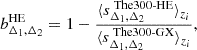
Here, we consider the case of X-ray and SZ observations of galaxy clusters providing measurements of the cluster mass at different overdensities under the hydrostatic equilibrium hypothesis. Observationally, HE masses are known to provide a biased measurement of the cluster mass as estimated, for instance, by lensing observations (see e.g. Pratt et al. 2019, for a review). Hydrodynamical simulations have been extensively used to investigate the amplitude and origin of the HE bias with respect to the true mass of simulated clusters (see e.g. Le Brun et al. 2017; Henson et al. 2017; Pearce et al. 2020; Ansarifard et al. 2020; Barnes et al. 2021; Kay et al. 2024; Braspenning et al. 2025). These studies have mainly focused on determining the mass and redshift evolution of the HE bias at fixed overdensity. However, a key question for sparsity analyses is how this bias varies across the mass profile. In fact, a radial-dependent mass bias will inevitably induce a bias on the estimated sparsity and propagate as a systematic error in the cosmological model parameter inference analyses. To assess such an effect, we use the HE mass estimates obtained in Gianfagna et al. (2023) from the spherically averaged properties of the intra-cluster medium of simulated clusters at different redshift snapshots from the GADGET-X runs. Their study has focused on the sample of most massive clusters in the zoomed-in simulated regions that do not contain any low-resolution particles within the virial radius, thus resulting in a sample of 290 clusters at z = 0. For each of these clusters, the HE masses at Δ = 200, 500, and 2500 have been determined using parametric fitting functions of the spherically averaged 3D pressure profile (as in the case of SZ-like observations of clusters), and the 3D gas density and temperature profiles (as in the case of X-ray cluster observations). We have used the data to compute the following set of sparsities:  ,
,  and
and  .
.
Firstly, we notice that the sparsities estimated using the X-ray masses have larger scatter than the SZ ones. Secondly, for each of the available redshifts, we found clusters with sparsities  , corresponding to
  , while estimates of the sparsities
  and
and  all lie above the physical threshold. These are shown in Fig. 10, where we plot s200, 500 from the X-ray (filled goldenrod squares) and SZ (empty blue circles) mass estimates against the true cluster mass M200 at z = 0.0, 0.5 and 1.0. As we can see 5 − 10% of the objects lie below the
  line and the number of such peculiar clusters is greater in the X-ray case than the SZ one. We verify that these cases are associated with disturbed systems that tend to have a negative bias (for which the HE mass is higher than the real mass) at R500 and a high positive bias at R200. In real data, this case could be present and may be the result from extrapolation of the fitting functions over regions that are not constrained by the data (see e.g. the case of HE masses of the HIFLUGCS clusters discussed in Corasaniti & Rasera 2019).
 |
Fig. 10. Sparsity s200, 500 estimated from the HE masses of the GADGET-X clusters from Gianfagna et al. (2023) at z = 0 (left panel), 0.5 (central panel) and 1.0 (right panel) using the X-ray temperature and gas density profiles (filled goldenrod squares) and SZ pressure profiles (empty blue circles). Values of s200, 500 ≤ 1 correspond to disturbed clusters for which the HE is not satisfied. Some of these are associated to systems with a vanishing or negative HE mass bias at R500 and a significant bias at R200. |
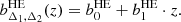
In the following, we exclude these clusters from the HE samples. Then, for each cluster we compare the HE estimated sparsities to those of the corresponding GADGET-X cluster and evaluate the HE sparsity bias7:
 (5)
(5)
where sΔ1, Δ2true is the sparsity obtained using the total 3D mass of the GADGET-X cluster. In Fig. 11, we plot the probability density function of the HE sparsity bias for the different overdensity pairs (panels from left to right) at z = 0.0 (top panels), 0.5 (central panels) and 1.0 (bottom panels) for the X-ray (blue bars) and SZ (red bars) mass estimates respectively. As we can see the distributions exhibit non-Gaussian tails, hence we use the mean, the median and the 16-th and 84-th percentiles as summary statistics.
 |
Fig. 11. Probability density function of the HE sparsity bias bs200, 500 (left columns), bs200, 2500 (central columns), and bs500, 2500 (right columns) for the X-ray (blue bars) and SZ (red bars) masses, respectively, at z = 0.07 (top rows), 0.46 (central rows), and 0.99 (bottom rows). |
5.1. Mass and redshift dependence
First, we investigate the dependence of the summary statistics on the mass of the simulated clusters. This is shown, in Fig. 12, where we plot the mean, the median and the 16-th and 84th percentiles of the HE bias for the three sparsity configuration considered as function of M200 for the samples at z = 0.0 (blue), 0.5 (magenta) and 1.0 (green) respectively. As we can see, the bias is largely independent of the mass enclosed within the outer radius probed by the sparsity. This is a direct consequence of the fact that the HE mass bias at different overdensity is independent of the cluster mass as found by several works in the literature in the high-mass range (see e.g. Le Brun et al. 2017; Henson et al. 2017; Pearce et al. 2020; Ansarifard et al. 2020; Barnes et al. 2021). We may also notice that there is no significant variation of the HE bias among the three different redshift samples, thus indicating a weak dependence on redshift.
 |
Fig. 12. HE sparsity bias bs200, 500 and bs200, 2500 as function of M200 (top panels) and bs500, 2500 as function of M500 (bottom panel) for the X (left panels) and SZ (right panels) masses of the full cluster sample at z = 0.0 (blue circles), 0.5 (magenta squares), and 1.0 (green stars). The different lines correspond to the median (solid) and the mean (dashed), while the shaded area to the region comprised between the 16th and 84th percentile. |
Indeed, concerning the redshift dependence we can see from Fig. 11 that in all the cases the mean, median and percentiles of the HE sparsity bias remain approximately constant as a function of redshift. Moreover, we remark that the biases from the X-ray masses (left panels) exhibit a larger scatter than those from the SZ masses (right panels). This is especially the case for bs200, 500SZ, that shows a level of scatter twice as small as that of bs200, 500X. This is consistent with the different level of scatter of the HE mass bias at Δ = 200 and 500 found in Gianfagna et al. (2023) for the X-ray and SZ cases respectively (see their Fig. 1).
In Tab. 3, we quote the values of the mean and median of the different HE sparsity bias estimated by merging together the different redshift samples, although we point out that joining the samples may introduce some spurious correlations from the repetition of objects which we cannot quantify. A point which will try to assess when evaluating the impact of such biases on the cosmological parameter inference analyses.
Mean and median (denoted as μ) of the hydrostatic sparsity bias.
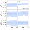 |
Fig. 13. Summary statistics of the HE sparsity bias bs200, 500 (top panels), bs200, 2500 (mid panels), and bs500, 2500 (bottom panels) as a function of redshift for the X (left panels) and SZ (right panels) masses. The different lines correspond to the median (solid) and mean (dashed), while the shaded area corresponds to the region comprised between the 16-th and 84-th percentile. |
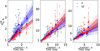 |
Fig. 14. HE sparsities sΔ1, Δ2HE from the X (blue) and SZ (red) catalogues with respect to their GADGET-X counterparts at z = 0 in the case of s200, 500 (left panel), s500, 2500(central panel), and s200, 2500 (right panel). The coloured dashed line correspond to the average linear fit to the 25 equally spaced binned data points (squares) in bins of true sparsities containing at least two clusters. The shaded areas indicates that 1 and 2σ credible regions. The black solid line corresponds to the unbiased case. |
5.2. HE sparsity versus true sparsity
Having discussed the summary statistics of the HE sparsity bias, it is worth investigating the relation between the true sparsities and the HE ones on a cluster-by-cluster basis. In Fig. 14, we plot the sparsities s200, 500 (left panel), s200, 2500 (central panel) and s500, 2500 (right panel) of the GADGET-X clusters from the X-ray (light blue circles) and SZ (light red circles) samples at z = 0 against the true sparsity values. For visual purposes, we plot the unbiased case as solid black lines. We also plot the mean of the X-ray (blue squares) and SZ (red squares) sparsities in 25 equally spaced bins of true sparsity values, where we have only retained the bins with more than two clusters. The errorbars represent the standard deviation. We find that a simple linear fit captures the relation between the true sparsities and HE ones, with a scatter that increases as function of true sparsity. We perform a Bayesian linear regression to infer the values of the slope mHE and the intercept cHE. The average linear fits are shown in Fig. 14 as dashed lines, while the shaded areas correspond the 1 and 2σ credible regions. The results show that the steeper the slope the greater the bias as well as the level of scatter. For instance, in the case of s200, 500, we can see that the SZ sparsities lies nearly parallel to the diagonal line with a small scatter. This is consistent with the low level of bias and reduced scatter we have found in the case of the SZ bias summary statistics shown in the top right panels of Figs. 12 and 13. This is not the case of the X-ray sparsities, for which the relation to the true sparsities has a steeper slope and greater scatter.
We have performed a similar regression at other redshifts and found no statistically significant trend, consistently with the results of the analysis of the summary statistics. We quote in Table 4 (Table 5) the inferred values of the fitting coefficients for the X (SZ) sparsities respectively. These fits provide a model for the intrinsic HE sparsity bias that is necessary to take into account in the case of cosmological parameter inference analyses the make use of individual cluster sparsity measurements as proposed in Richardson & Corasaniti (2023), an approach that we do not consider here.
Bayesian linear regression coefficients strue versus sX relation.
Bayesian linear regression coefficients strue versus sSZ relation.
6. Cosmological implications
In light of the analyses presented in the previous sections, it is of interest to evaluate the implications of the sparsity bias on cosmological analyses performed using this type of measurement. For instance, Corasaniti et al. (2018, 2021), and Richardson & Corasaniti (2023) propose different approaches to use the sparsities of galaxy clusters to constrain cosmology. These methodologies rely on either comparing the mean sparsity of a sample of clusters or the individual sparsities within the sample to a theoretical prediction computed from the halo mass function, and are therefore susceptible to the biases presented above.
At the time of writing, sparsity constraints remain reliant on predictions from N-body simulations (e.g. Despali et al. 2016; Rasera et al. 2022) as the high-mass regime of the halo mass function remains poorly constrained in the presence of baryonic physics. This is primarily due to the computational cost of running simulations of a sufficiently large volume to accurately capture the cut-off at high masses with only a few hydrodynamical cosmological simulations being able to reach box side lengths of the order of a few h−1 Gpc, e.g Magneticum8 (Dolag et al. 2016), Millenium TNG9 (Pakmor et al. 2023) and FLAMINGO10 (Schaye et al. 2023).
In the following, we perform a number of analyses using the approach of Corasaniti et al. (2018) to assess the impact of HE sparsity bias and selection effects on the cosmological parameter inferences. Before presenting the methods along with the additional corrections to account for such effects, we first present the synthetic datasets we have used for these analyses.
6.1. Synthetic sparsity data and calibration samples
We generate two distinct synthetic datasets consisting of different cluster sparsity catalogues, which we use to assess the impact of systematic biases.
The first dataset consists of clusters from the GADGET-X simulation. To avoid the repetition of clusters in the sample, we first select 277 GADGET-X clusters with redshifts randomly drawn from the set of eight redshift snapshots of the GADGET-X simulation for which the X-ray and SZ masses are computed. We subsequently assign to each cluster the mass estimates corresponding to that redshift. In doing so, we generate three different catalogues: one consisting of cluster sparsities obtained using the hydro masses from the GADGET-X simulation: two others are generated using HE mass estimates from Gianfagna et al. (2023). We refer to these catalogues as the The300-GX, The300-X and The300-SZ respectively.
The second dataset consists of haloes from the UCHUU N-body simulation (Ishiyama et al. 2021) described in Sec. 2.2.2. In particular, we first identify all haloes in the catalogues with masses M200 > 1014 h−1 M⊙, in all snapshots at z ≤ 1.22. Then, we randomly draw 277 haloes with redshift from the UCHUU snapshots that are the closest to those of the The300 in terms of redshift. In building such a dataset, we verify that no halo is selected multiple times by checking that the haloes are sufficiently far away. For example, the two closest haloes are 40 h−1 Mpc apart (not accounting for the redshift difference). Indeed, the purpose of the UCHUU synthetic dataset is twofold. Firstly, it provides a dataset with a minimal amount of selection bias since, as shown in Corasaniti et al. (2018, 2021), Richardson & Corasaniti (2023), a random selection of haloes with a mass cut-off does not induce a considerable bias to the estimation of the sparsity statistics. Secondly, it provides a dataset for which the effect of selection bias is well constrained and as such it allows us to verify that the bias model correction we add to the likelihoods performs correctly.
Having generated these datasets, we split each of the catalogues into two separate subsamples by randomly selecting 100 clusters to form a data subsample, which is used for the cosmological parameter inference; while the remaining 177 clusters constitute a calibration subsample, which we further bootstrap to calibrate statistical models of the different bias effects.
6.2. Cosmological model predictions
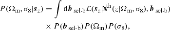
We predict the mean sparsity of the data for a given cosmological model using the integral relation (Balmès et al. 2014; Richardson & Corasaniti 2023):
 (6)
(6)
which links the Halo Mass Function (HMF) at two distinct spherical overdensity contrasts,  and
and  , to the mean sparsity of the sample, ⟨sΔ1, Δ2⟩. Given the functional form of the HMFs, this equation can be solved numerically with integration boundaries which reflect the data sample. In the case at hand, this means choosing an arbitrarily high upper bound, due to the exponential cut-off in the HMF, and a lower bound corresponding to the smallest cluster in the sample,
  . For the HMF model, we choose to recalibrate the Despali et al. (2016) HMF on the large volume UCHUU simulation (Ishiyama et al. 2021), see Appendix B for details. It is important to note that we also include a redshift dependent correction to the predicted sparsities to account for the HMF fitting inaccuracies. In particular, the correction to the mean sparsity takes the form of a multiplicative term,
 (7)
(7)
 (8)
(8)
 (9)
(9)
such that 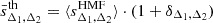 , where ⟨sΔ1, Δ2HMF⟩ is inferred from Eq. (6). These terms are required due to the rigidity of the Despali et al. (2016) fitting function at high masses which does not capture the high mass cut-off in the HMF with sufficient accuracy, which is particularly visible in Fig. B.3. These terms are obtained by fitting the residuals between the mean sparsity of the UCHUU-DM calibration sample and that predicted by Eq. (6). For illustrative purposes, we plot in Fig. 15 the predicted
  for the Uchuu’s fiducial cosmology against the UCHUU-DM data.
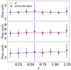 |
Fig. 15. Mean sparsities predicted by Eq. (6) with the redshift-dependent corrections (solid red lines) for the Uchuu fiducial cosmology against the estimates of the means from the UCHUU-DM data sample in equally spaced redshift bins (blue squares). |
6.3. Bias models
6.3.1. Selection and baryon bias
As briefly mentioned, it has been shown that a random selection with a mass cut has a minimal impact on the cosmological parameter inferences using sparsity (Corasaniti et al. 2018, 2021; Richardson & Corasaniti 2023). While this type of selection is easily achievable when using data from a large volume cosmological simulation, this is generally not the case in most observational settings. For instance, the clusters from the Tier-1 CHEX-MATE observational programme (CHEX-MATE Collaboration 2021), while offering a random selection of clusters with masses in the range 2 < M500 [1014 M⊙]< 9 and redshift 0.05 < z < 0.2, are still reliant on the Planck SZ selection function (Planck Collaboration XXIV 2016). Similarly, the Tier-2 CHEX-MATE observational programme, which has observed the most massive systems with M500 > 7.25 ⋅ 1014 M⊙, at low redshift, z < 0.6, is not only reliant on the Planck SZ selection function but also introduces its own selection.
The use of The300 sample poses a similar problem, since the selection of a subset of the ∼300 most massive clusters in the MDPL2 simulation at a random point in their mass assembly history is highly non-trivial. As already mentioned, to quantify the magnitude of this effect, we have generated a synthetic dataset to replicate the selection process described above using the halo catalogues of the UCHUU simulation (Ishiyama et al. 2021). This simulation has a volume eight times larger than the MDPL2 simulation, thus we can replicate the selection eight times without overlapping the sub-volumes. From each of the UCHUU sub-volumes, we select the 277 most massive objects to which, we randomly assign a redshift of observation, and recover the state of the halo at that redshift using the ROCKSTAR merger trees. Again, the redshifts are drawn from the set of the UCHUU snapshots whose redshifts are closest to those of The300. Finally, as already stated in Sec. 6.1, we randomly assign 100 haloes to a data sample and place the remaining haloes in a calibration sample. Since we aim to compare this selection to a purely random selection, we repeat this process by randomly selecting haloes with a mass M200 > 1014 h−1 M⊙ within each sub-volume. We bin the resulting datasets into eight redshift bins corresponding to the eight snapshots from which the cluster properties are drawn and compute the mean sparsities in each bin.
We compare these estimates to the mean sparsities from the The300-GX sample at the same redshifts. Notice that as we are comparing results from a DM-only simulation against those from hydrodynamical runs, the comparison provides us with an estimate of bias due to selection as well as the effect of baryons on the cluster sparsities discussed in Section 3.2.1. Specifically, we compute the selection-baryon bias:
 (10)
(10)
For conciseness, we show the mean and standard deviation for the different sparsity configurations at different redshifts in Fig. C.1 of Appendix C. In all the cases, we find the data points to be consistent with a constant trend in redshift, though a linear model,
 (11)
(11)
provides a better fit to the bias estimates, especially in the case of  and
and  . Henceforth, we infer the average and 1σ uncertainty of the fitting coefficients b0sel-b and b1sel-b through a Bayesian regression analysis for each sparsity configuration. The corresponding values are quoted in Table 6. Indeed, we may notice that slopes are consistent with zero within the 1σ errors. Nevertheless, to be as conservative as possible, we model the selection-baryon bias in terms of Eq. (11).
Linear regression coefficients of the selection-baryon bias model.
6.3.2. HE sparsity bias
We use the calibration samples from The300-X and The300-SZ datasets to estimate the HE bias by comparing the mean sparsities in different redshift bins against those estimated using The300-GX calibration sample. Namely, we compute
 (12)
(12)
and estimate the average and standard deviation for the different sparsity configurations at different redshift for the X-ray and SZ calibration samples. We find that the estimates are consistent with a constant redshift bias, though a linear redshift dependence can provide a better fit. Again, as in the case of the selection-baryon bias, to be as conservative as possible, we model these trends with a linear regression model:
 (13)
(13)
In Fig. C.2 of Appendix C, we show the HE bias estimates for the different sparsity configuration and the average linear regression fit, the 1 and 2σ credible regions, while in Table 7, we quote the average and 1σ uncertainty on the fitting coefficients b0HE and b1HE.
 |
Fig. 16. Bayesian graph models representing the relation between the cosmological parameters (Ωm, S8), the mean sparsity model prediction at a given redshift ( |

6.4. Cosmological parameter inference analyses
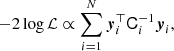
We are now able to investigate the impact of the different bias effects on the cosmological parameter constraints inferred from the analysis of mean sparsity measurements at different redshifts. Following the approach presented in Corasaniti et al. (2018), we infer constraints using mean sparsity measurements from a single overdensity configuration at different redshifts, ⟨s200, 500⟩, as well as from the combination of multiple sparsity configurations, {⟨s200, 500⟩,⟨s200, 2500⟩,⟨s500, 2500⟩}, as described in and Corasaniti et al. (2022). To this purpose we use the synthetic data samples generated in Sec. 6.1. We summarise the results in terms of the constraints on the parameter 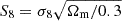 , which we infer by performing a Markov Monte Carlo chain sampling of the posterior distribution assuming uniform priors on Ωm ∈ [0.2, 0.6], and σ8 ∈ [0.2, 1.2]. We have set the remaining cosmological parameters to the fiducial values of the Planck cosmology.
Next, we discuss the propagation of the bias model uncertainties and the priors assumed on the bias model parameters.
6.5. Bayesian graph models
A schematic summary of the computation of posterior distribution adopted under different bias model assumptions is given by the Bayesian graphs shown in Fig. 16.
Panel a corresponds to the simplest case, where we neglect any bias effect. Hence, the posterior reads simply as:
 (14)
(14)
where ℒ is the likelihood function with sz being the data vector of mean sparsity measurements at different redshifts and  the vector of mean sparsity predictions, while P(Ωm) and P(σ8) are the prior distributions of the sampled parameters. In the case of a multiple sparsity dataset, sz = {s200, 500, s200, 2500, s500, 200}, while for a single sparsity this reduced to sz = {s200, 500}. Assuming a Gaussian likelihood function, the log-likelihood reads as:
 (15)
(15)
where N is the number of redshift bins, and
 (16)
(16)
The matrix Cz is accounts for the covariance between the different sparsities at a given redshift. In the case of a single sparsity statistics, this reduces to the intrinsic variance of the estimated sparsity, σszi2. In the case of multiple sparsities, we compute the covariance matrix using the correlation matrix between different sparsity configurations, rsα, sβz, as given by the analytical formulae derived in Corasaniti et al. (2022) using the M2Csims simulations (see Appendix D), such that Csα, sβz = σsαzσsβzrsα, sβz.
Panel b summarises the sampling of the posterior marginalised over the selection-baryon bias model:
 (17)
(17)
where P(bsel-b) is the prior distribution of the selection-baryon bias model parameters. In such a case, we assume the linear redshift dependent bias model Eq. (11), such that
![Mathematical equation: $$ \begin{aligned} \boldsymbol{\bar{s}}^\mathrm{th}(z)\rightarrow \left[1-\boldsymbol{b}_{\text{ sel-b}}(z)\right]\cdot \boldsymbol{\bar{s}}^\mathrm{th}(z). \end{aligned} $$](/articles/aa/full_html/2025/05/aa53914-25/aa53914-25-eq74.gif) (18)
(18)
In sampling the posterior distribution, Eq. (17), we assume Gaussian priors for the selection-baryon bias parameters  and
and  of each sparsity configuration, with mean and standard deviation specified by the values quoted in Table 6.
Finally, panel c shows the Bayesian graph for the sampling of the posterior in the presence of the selection-baryon bias and the HE bias:
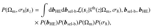 (19)
(19)
where P(bHE) is the prior distribution of the HE bias model parameters. We assume the linear HE bias model given by Eq. (5), hence to leading order in the bias parameters we have
![Mathematical equation: $$ \begin{aligned} \boldsymbol{\bar{s}}^\mathrm{th}(z)\rightarrow \left[1-\boldsymbol{b}_{\rm HE}(z)-\boldsymbol{b}_{\text{ sel-b}}(z)\right]\cdot \boldsymbol{\bar{s}}^\mathrm{th}(z). \end{aligned} $$](/articles/aa/full_html/2025/05/aa53914-25/aa53914-25-eq78.gif) (20)
(20)
In sampling the posterior distribution, Eq. (19), in addition to the Gaussian priors on the selection bias parameters, we also assume Gaussian priors for the HE bias parameters of each sparsity configuration with mean and standard deviation specified by the values given in Table 7.
Linear regression coefficients of the HE bias model.
6.6. Results
Here, we present the results of the MCMC likelihood analysis of the UCHUU-DM, The300-GX, The300-X and The300-SZ synthetic data samples in the case of s200, 500 (1S) and multiple (3S) average sparsity measurements. We summarise the results in terms of the constraints on the parameter S8 and remind the reader that the synthetic datasets have been generated with a fiducial value S8f = 0.83. The marginalised constraints are quoted in Table 8, where we report the mean and 1σ uncertainty, as well as the best-fit values of S8 as inferred under the different data models described in the previous section. The marginalised posteriors are shown in Figs. 17 and 18 respectively.
Marginalised constraints on S8.
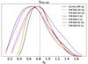 |
Fig. 17. Marginalised posterior on S8 from the analysis of single sparsity measurements for the UCHUU-DM (black curve), The300-GX (yellow curves), The300-X (blue curves) and The300-SZ (red curves). The solid lines represent posterior inferred with the simplest data model, while the dashed lines corresponds to posteriors obtained marginalising over bias model parameters. |
The analysis of the UCHUU-DM data sample provides us with a reference benchmark, since the cosmological model predictions obtained from Eq. (6) have been calibrated using the UCHUU halo catalogues. In Figs. 17 and 18, we plot the corresponding posterior distributions (solid black lines) inferred using the Bayesian model specified by Eq. (14) in the 1S and 3S case respectively. We can see that the peak of the distributions lies close to the fiducial value. Moreover, we may notice from the values quoted in Table 8 that S8f = 0.83 lies well within the 1σ estimated errors. Quite importantly, we can see the constraint from the 3S analysis is nearly a factor of 2 more stringent than the 1S, consistently with the results of Corasaniti et al. (2022).
The analysis of The300-GX data sample provides us with an estimate of the impact of the selection-baryon bias on the cosmological parameter inference. In particular, we can see from Fig. 17 that in the 1S case, the posterior distribution (solid yellow line) obtained using the basic data model Eq. (14) is only slightly shifted with respect to the benchmark posterior. This is consistent with the fact that the level of selection-baryon bias on s200, 500 is of the order of a few percent with respect to the DM-only case. We find S8f to be within the 1σ credible interval. This is not the case of the 3S analysis, for which where the effect of neglecting the selection-baryon bias is significantly larger, with S8f excluded at more than 2σ. Instead, marginalising over the bias model, as specified by Eq. (17), results in unbiased constraints both in the 1S and 3S case. Though the inferred bounds on S8 are weaker than those inferred in the benchmark case, a direct consequence of the marginalisation on the bias model parameters.
In Figs. 17 and 18, we plot the marginalised posterior from the 1S and 3S analysis of The300-X (blue lines) and The300-SZ (red lines) data samples. We first perform a likelihood analysis only accounting for the selection-baryon bias model as in Eq. (17). We find posterior distributions that are systematically biased towards low S8 values (solid curves). The effect is significantly more important for the 3S analysis than the 1S, as it can also be noticed from the values quoted in Table 8. In particular, in the 1S case the fiducial value remains within the 1σ errors, while it is excluded at more than 2σ for the 3S case. In contrast, accounting for the HE bias, as specified by Eq. (19), results in unbiased constraints. We can see that the marginalised posterior distributions (dashed lines) peak close to the fiducial value and overlap with the benchmark distribution. We stress the fact that the use of multiple average sparsity measurements always lead to tighter bounds on S8. After marginalising over the bias parameters, the joint analysis of s200, 500, s200, 2500 and s500, 2500 removes projection effects that limits the bound inferred using s200, 500 only. In particular, the joint analysis results in a constraint on S8 that is a factor ∼2.6 tighter in the case of the X-ray data sample and ∼3.6 for the SZ one.
7. Conclusions
Halo sparsity is a simple, non-parametric proxy of the distribution of mass within haloes hosting galaxy groups and clusters (Balmès et al. 2014). Being a ratio of masses estimated at radii which enclose different overdensities, it provides an estimate of the local logarithmic slope of the halo mass profile that encodes cosmological information resulting from the halo mass assembly history. For a given cosmological setup, the statistical properties of the halo sparsity can be estimated using cosmological N-body simulations. These can in turn be used to calibrate analytical relations to predict the average sparsity at different redshifts and for different overdensity pairs for a given cosmological model (Corasaniti et al. 2018; Corasaniti & Rasera 2019; Corasaniti et al. 2022). This has opened up the possibility to perform cosmological parameter inference analyses using sparsity measurements in clusters. However, with the increasing precision of cluster mass estimates, it has become critical to assess potential sources of systematic error. In particular, given that the prediction relies on DM-only simulations, it is important to assess the impact of baryons on the predicted sparsities and more generally the effects of selection and mass estimation biases. Here, we have investigated these potential sources of systematic uncertainty using the simulated clusters from the The300 zoom-in simulation suite (Cui et al. 2018, 2022). Furthermore, we use hydrostatic equilibrium masses estimated from 3D ICM thermodynamic profiles of The300 clusters by Gianfagna et al. (2023) to assess the effect of HE mass bias.
First, we find that the presence of baryons in simulated clusters alters the sparsity relative to DM-only predictions differently at different overdensities. In particular, the further two radii are from one another, the larger the differential change will be with respect to the DM-only sparsities. This is consistent with expectations from the baryon-induced radial-dependent mass bias found in simulated clusters (e.g. Biffi et al. 2016; Le Brun et al. 2017). Moreover, we find that the amplitude of this bias is directly correlated with the strength of the baryonic feedback implemented in the simulations, with stronger feedback models leading to a larger sparsity bias. Nevertheless, on average the effect remains minimal (at a few percent level) for sparsities probing the external cluster regions, such as s200, 500, while it is maximal at large overdensities, such as s200, 2500. Quite importantly, the scatter around the average bias strongly depends on the dynamical state of the simulated clusters.
Given the sensitivity of certain sparsity configurations to the astrophysical processes that shape the properties of the baryonic gas in clusters, we investigate the relation between sparsities and the gas fraction. We find a moderate anti-correlation (∼40%−60%) between the gas fraction within the inner cluster regions and the sparsities s200, 500 and s500, 2500 respectively. In particular, we find that the lower the value of the gas fraction inside the shell comprised between R2500 and R500, and the higher the value of the sparsity s500, 2500. This is a direct consequence of the effect of AGN on the gas and total mass distribution in clusters. On the other hand, we find that gas fraction measured within R500 weakly correlate with the sparsity s200, 500 and s500, 2500, thus carrying complementary information that can be exploited for joint cosmological analyses. Furthermore, we find that ratios of the gas fraction estimated at different overdensities provide a bias tracer of the cluster sparsity, which is particularly sensitive to the underlying astrophysical feedback model implemented in the simulations.
Using the HE mass estimates of The300 cluster sample from Gianfagna et al. (2023), we study the impact of the HE mass bias on sparsity measurements. In particular, we find a median bias which ranges from a few to a maximum of 10% level depending on the sparsity configuration. Moreover, we find that HE mass inferred from X-ray data leads to a larger scatter of the sparsity bias than SZ ones.
Finally, we generate synthetic datasets to estimate the joint effect of selection, baryon and HE bias on the cosmological parameter constraints inferred from single and multiple average sparsity measurements. By splitting the datasets into calibration and data samples, we use the former to calibrate linear redshift dependent models of the various sources of bias; whereas we use the data samples, consisting of sparsity measurements of 100 clusters in the redshift range 0 < z < 1.2, to perform a MCMC likelihood analysis and derive constraints on S8 under different data model assumptions. We find that the effect of the sparsity biases is to systematically shift the posteriors towards lower S8 values. In the case of single sparsity measurements (s200, 500), the effect is small and well within the statistical uncertainties. In contrast, the joint analysis of multiple sparsity measurements (s200, 500, s200, 2500 and s500, 2500) result in a larger systematic effect with the fiducial S8 value excluded at more than 2σ. We show that calibrated linear redshift dependent bias models can be used to account for such sparsity biases and marginalising over the sparsity bias model parameters is sufficient to recover the fiducial cosmology and infer unbiased constraints on S8. The evaluation of the HE and selection mass biases presented in this study can be further improved through the analysis of a randomly selected cosmological samples of simulated clusters with 2D de-projected HE mass estimates.
In the case of application to observational data, one could calibrate the sparsity bias model parameters and propagate them through the cosmological parameter inference using the same methodology we have presented in this work. For instance, subsamples of data for which HE and lensing masses are measured at different overdensities could be used to calibrate the HE bias model parameters of different sparsity configurations, allowing to also capture projection effects. Similarly, one could estimate selection effects as in standard data analyses by comparing to random mocks.
Alternatively, the halo sparsity can be seen as an indirect proxy of the logarithmic steepness of the radial halo mass profile, since
 (2)
(2)
The fact that the sparsities are by definition strictly larger than unity does not imply that the gas mass fraction ratios have to be greater than one, since there is no physical reason to prevent sΔ1, Δ2gas < sΔ1, Δ2. Indeed, a few clusters in the sample have such values.
Notice that Eq. (5) can be written in terms of the HE mass bias of a given cluster at overdensity Δ1 and Δ2 respectively:
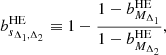 (4)
(4)
where  .
.
Acknowledgments
This work has been made possible by The Three Hundred collaboration (https://www.the300-project.org). The authors acknowledge The Red Española de Supercomputación for granting computing time for running most of the hydrodynamical simulations of THE THREE HUNDRED galaxy cluster project in the Marenostrum supercomputer at the Barcelona Supercomputing Center. P.S.C., A.M.C.L.B. and Y.R. acknowledge support from CNES (Centre National d’Etudes Spatiales). T.R. acknowledge funding from the Spanish Goverment’s grant programme “Proyectos de Generación de Conocimiento” under grant number PID2021-128338NB-I00. M.D.P. acknowledges financial support from PRIN-MIUR grant 20228B938N “Mass and selection biases of galaxy clusters: a multi-probe approach” funded by the European Union Next generation EU, Mission 4 Component 1 CUP C53D2300092 0006. S.E. acknowledges the financial contribution from the contracts Prin-MUR 2022 supported by Next Generation EU (M4.C2.1.1, n.20227RNLY3 The concordance cosmological model: stress-tests with galaxy clusters), and from the European Union’s Horizon 2020 Programme under the AHEAD2020 project (grant agreement n. 871158). W.C. and G.Y. would like to thank Ministerio de Ciencia e Innovación for financial support under project grant PID2021-122603NB-C21. W.C. is supported by the Atracción de Talento Contract no. 2020-T1/TIC-19882 granted by the Comunidad de Madrid in Spain. W.C. also thanks the ERC: HORIZON-TMA-MSCA-SE for supporting the LACEGAL-III project with grant number 101086388 and the China Manned Space Project for its research grants. The CosmoSim database used in this paper is a service by the Leibniz-Institute for Astrophysics Potsdam (AIP). The MultiDark database was developed in cooperation with the Spanish Multi-Dark Consolider Project CSD2009-00064. The authors gratefully acknowledge the Gauss Centre for Supercomputing e.V. (www.gauss-centre.eu) and the Partnership for Advanced Supercomputing in Europe (PRACE, www.prace-ri.eu) for funding the MultiDark simulation project by providing computing time on the GCS Supercomputer SuperMUC at Leibniz Supercomputing Centre (LRZ, www.lrz.de). The authors also thank the Instituto de Astrofisica de Andalucia (IAA-CSIC), Centro de Supercomputacion de Galicia (CESGA) and the Spanish academic and research network (RedIRIS) in Spain for hosting UCHUU DR1, DR2 and DR3 in the Skies & Universes site for cosmological simulations. The UCHUU simulations were carried out on Aterui II supercomputer at Center for Computational Astrophysics, CfCA, of National Astronomical Observatory of Japan, and the K computer at the RIKEN Advanced Institute for Computational Science. The UCHUU Data Releases efforts have made use of the skun@IAA_RedIRIS and skun6@IAA computer facilities managed by the IAA-CSIC in Spain (MICINN EU-Feder grant EQC2018-004366-P).
References
- Allen, S. W., Evrard, A. E., & Mantz, A. B. 2011, ARA&A, 49, 409 [Google Scholar]
- Angelinelli, M., Ettori, S., Dolag, K., Vazza, F., & Ragagnin, A. 2023, A&A, 675, A188 [NASA ADS] [CrossRef] [EDP Sciences] [Google Scholar]
- Ansarifard, S., Rasia, E., Biffi, V., et al. 2020, A&A, 634, A113 [NASA ADS] [CrossRef] [EDP Sciences] [Google Scholar]
- Balmès, I., Rasera, Y., Corasaniti, P. S., & Alimi, J. M. 2014, MNRAS, 437, 2328 [CrossRef] [Google Scholar]
- Barnes, D. J., Vogelsberger, M., Pearce, F. A., et al. 2021, MNRAS, 506, 2533 [NASA ADS] [CrossRef] [Google Scholar]
- Battaglia, N., Bond, J. R., Pfrommer, C., & Sievers, J. L. 2013, ApJ, 777, 123 [NASA ADS] [CrossRef] [Google Scholar]
- Beck, A. M., Murante, G., Arth, A., et al. 2016, MNRAS, 455, 2110 [Google Scholar]
- Behroozi, P. S., Wechsler, R. H., & Wu, H.-Y. 2013, ApJ, 762, 109 [NASA ADS] [CrossRef] [Google Scholar]
- Biffi, V., Borgani, S., Murante, G., et al. 2016, ApJ, 827, 112 [NASA ADS] [CrossRef] [Google Scholar]
- Bocquet, S., Dietrich, J. P., Schrabback, T., et al. 2019, ApJ, 878, 55 [Google Scholar]
- Braspenning, J., Schaye, J., Schaller, M., Kugel, R., & Kay, S. T. 2025, MNRAS, 536, 3784 [Google Scholar]
- Bryan, G. L., & Norman, M. L. 1998, ApJ, 495, 80 [NASA ADS] [CrossRef] [Google Scholar]
- Bullock, J. S., Kolatt, T. S., Sigad, Y., et al. 2001, MNRAS, 321, 559 [Google Scholar]
- CHEX-MATE Collaboration (Arnaud, M., et al.) 2021, A&A, 650, A104 [NASA ADS] [CrossRef] [EDP Sciences] [Google Scholar]
- Corasaniti, P. S., & Rasera, Y. 2019, MNRAS, 487, 4382 [Google Scholar]
- Corasaniti, P. S., Ettori, S., Rasera, Y., et al. 2018, ApJ, 862, 40 [CrossRef] [Google Scholar]
- Corasaniti, P. S., Giocoli, C., & Baldi, M. 2020, Phys. Rev. D, 102, 043501 [Google Scholar]
- Corasaniti, P.-S., Sereno, M., & Ettori, S. 2021, ApJ, 911, 82 [NASA ADS] [CrossRef] [Google Scholar]
- Corasaniti, P. S., Le Brun, A. M. C., Richardson, T. R. G., et al. 2022, MNRAS, 516, 437 [NASA ADS] [CrossRef] [Google Scholar]
- Cui, W., Knebe, A., Yepes, G., et al. 2018, MNRAS, 480, 2898 [Google Scholar]
- Cui, W., Dave, R., Knebe, A., et al. 2022, MNRAS, 514, 977 [NASA ADS] [CrossRef] [Google Scholar]
- Davé, R., Anglés-Alcázar, D., Narayanan, D., et al. 2019, MNRAS, 486, 2827 [Google Scholar]
- De Luca, F., De Petris, M., Yepes, G., et al. 2021, MNRAS, 504, 5383 [NASA ADS] [CrossRef] [Google Scholar]
- Despali, G., Giocoli, C., Angulo, R. E., et al. 2016, MNRAS, 456, 2486 [NASA ADS] [CrossRef] [Google Scholar]
- Dolag, K., Bartelmann, M., Perrotta, F., et al. 2004, A&A, 416, 853 [NASA ADS] [CrossRef] [EDP Sciences] [Google Scholar]
- Dolag, K., Komatsu, E., & Sunyaev, R. 2016, MNRAS, 463, 1797 [Google Scholar]
- Duffy, A. R., Schaye, J., Kay, S. T., et al. 2010, MNRAS, 405, 2161 [NASA ADS] [Google Scholar]
- Eckert, D., Ettori, S., Molendi, S., Vazza, F., & Paltani, S. 2013, A&A, 551, A23 [NASA ADS] [CrossRef] [EDP Sciences] [Google Scholar]
- Ettori, S., Dolag, K., Borgani, S., & Murante, G. 2006, MNRAS, 365, 1021 [NASA ADS] [CrossRef] [Google Scholar]
- Ettori, S., Morandi, A., Tozzi, P., et al. 2009, A&A, 501, 61 [NASA ADS] [CrossRef] [EDP Sciences] [Google Scholar]
- Ettori, S., Gastaldello, F., Leccardi, A., et al. 2010, A&A, 524, A68 [NASA ADS] [CrossRef] [EDP Sciences] [Google Scholar]
- Euclid Collaboration (Adam, R., et al.) 2019, A&A, 627, A23 [NASA ADS] [CrossRef] [EDP Sciences] [Google Scholar]
- Frenk, C. S., White, S. D. M., Bode, P., et al. 1999, ApJ, 525, 554 [Google Scholar]
- Gianfagna, G., Rasia, E., Cui, W., et al. 2023, MNRAS, 518, 4238 [Google Scholar]
- Giocoli, C., Tormen, G., & Sheth, R. K. 2012, MNRAS, 422, 185 [NASA ADS] [CrossRef] [Google Scholar]
- Gnedin, O. Y., Kravtsov, A. V., Klypin, A. A., & Nagai, D. 2004, ApJ, 616, 16 [Google Scholar]
- Haggar, R., Gray, M. E., Pearce, F. R., et al. 2020, MNRAS, 492, 6074 [NASA ADS] [CrossRef] [Google Scholar]
- Henson, M. A., Barnes, D. J., Kay, S. T., McCarthy, I. G., & Schaye, J. 2017, MNRAS, 465, 3361 [NASA ADS] [CrossRef] [Google Scholar]
- Hopkins, P. F. 2015, MNRAS, 450, 53 [Google Scholar]
- Ishiyama, T., Fukushige, T., & Makino, J. 2009, PASJ, 61, 1319 [NASA ADS] [CrossRef] [Google Scholar]
- Ishiyama, T., Nitadori, K., & Makino, J. 2012, ArXiv e-prints [arXiv:1211.4406] [Google Scholar]
- Ishiyama, T., Prada, F., Klypin, A. A., et al. 2021, MNRAS, 506, 4210 [NASA ADS] [CrossRef] [Google Scholar]
- Kay, S. T., Braspenning, J., Chluba, J., et al. 2024, MNRAS, 534, 251 [Google Scholar]
- King, L. J., & Mead, J. M. G. 2011, MNRAS, 416, 2539 [Google Scholar]
- Kitayama, T., & Suto, Y. 1996, MNRAS, 280, 638 [NASA ADS] [Google Scholar]
- Klypin, A., Yepes, G., Gottlöber, S., Prada, F., & Heß, S. 2016, MNRAS, 457, 4340 [Google Scholar]
- Knollmann, S. R., & Knebe, A. 2009, ApJS, 182, 608 [Google Scholar]
- Kravtsov, A. V., & Borgani, S. 2012, ARA&A, 50, 353 [Google Scholar]
- Kullback, S., & Leibler, R. A. 1951, The Annals of Mathematical Statistics, 22, 79 [Google Scholar]
- Le Brun, A. M. C., McCarthy, I. G., Schaye, J., & Ponman, T. J. 2017, MNRAS, 466, 4442 [Google Scholar]
- Lee, C. T., Primack, J. R., Behroozi, P., et al. 2017, MNRAS, 466, 3834 [CrossRef] [Google Scholar]
- Lesci, G. F., Marulli, F., Moscardini, L., et al. 2022, A&A, 659, A88 [NASA ADS] [CrossRef] [EDP Sciences] [Google Scholar]
- Ludlow, A. D., Navarro, J. F., Li, M., et al. 2012, MNRAS, 427, 1322 [NASA ADS] [CrossRef] [Google Scholar]
- Ludlow, A. D., Navarro, J. F., Boylan-Kolchin, M., et al. 2013, MNRAS, 432, 1103 [NASA ADS] [CrossRef] [Google Scholar]
- Macciò, A. V., Dutton, A. A., van den Bosch, F. C., et al. 2007, MNRAS, 378, 55 [Google Scholar]
- Mantz, A. B., Allen, S. W., Morris, R. G., et al. 2014, MNRAS, 440, 2077 [NASA ADS] [CrossRef] [Google Scholar]
- Mantz, A. B., Allen, S. W., Morris, R. G., & Schmidt, R. W. 2016, MNRAS, 456, 4020 [NASA ADS] [CrossRef] [Google Scholar]
- Mantz, A. B., Morris, R. G., Allen, S. W., et al. 2022, MNRAS, 510, 131 [Google Scholar]
- Martizzi, D., Teyssier, R., Moore, B., & Wentz, T. 2012, MNRAS, 422, 3081 [NASA ADS] [CrossRef] [Google Scholar]
- Marulli, F., Veropalumbo, A., García-Farieta, J. E., et al. 2021, ApJ, 920, 13 [Google Scholar]
- Mead, J. M. G., King, L. J., Sijacki, D., et al. 2010, MNRAS, 406, 434 [Google Scholar]
- Navarro, J. F., Frenk, C. S., & White, S. D. M. 1997, ApJ, 490, 493 [Google Scholar]
- Neto, A. F., Gao, L., Bett, P., et al. 2007, MNRAS, 381, 1450 [NASA ADS] [CrossRef] [Google Scholar]
- Pacaud, F., Pierre, M., Melin, J. B., et al. 2018, A&A, 620, A10 [NASA ADS] [CrossRef] [EDP Sciences] [Google Scholar]
- Pakmor, R., Springel, V., Coles, J. P., et al. 2023, MNRAS, 524, 2539 [NASA ADS] [CrossRef] [Google Scholar]
- Pearce, F. A., Kay, S. T., Barnes, D. J., Bower, R. G., & Schaller, M. 2020, MNRAS, 491, 1622 [NASA ADS] [CrossRef] [Google Scholar]
- Planck Collaboration XX. 2014, A&A, 571, A20 [NASA ADS] [CrossRef] [EDP Sciences] [Google Scholar]
- Planck Collaboration XXI. 2014, A&A, 571, A21 [NASA ADS] [CrossRef] [EDP Sciences] [Google Scholar]
- Planck Collaboration XIII 2016, A&A, 594, A13 [NASA ADS] [CrossRef] [EDP Sciences] [Google Scholar]
- Planck Collaboration XXIV. 2016, A&A, 594, A24 [NASA ADS] [CrossRef] [EDP Sciences] [Google Scholar]
- Planelles, S., Borgani, S., Dolag, K., et al. 2013, MNRAS, 431, 1487 [Google Scholar]
- Prada, F., Klypin, A. A., Cuesta, A. J., Betancort-Rijo, J. E., & Primack, J. 2012, MNRAS, 423, 3018 [NASA ADS] [CrossRef] [Google Scholar]
- Pratt, G. W., Arnaud, M., Piffaretti, R., et al. 2010, A&A, 511, A85 [NASA ADS] [CrossRef] [EDP Sciences] [Google Scholar]
- Pratt, G. W., Arnaud, M., Biviano, A., et al. 2019, Space Sci. Rev., 215, 25 [Google Scholar]
- Rasera, Y., Breton, M. A., Corasaniti, P. S., et al. 2022, A&A, 661, A90 [NASA ADS] [CrossRef] [EDP Sciences] [Google Scholar]
- Rasia, E., Tormen, G., & Moscardini, L. 2004, MNRAS, 351, 237 [NASA ADS] [CrossRef] [Google Scholar]
- Rasia, E., Borgani, S., Ettori, S., Mazzotta, P., & Meneghetti, M. 2013, ApJ, 776, 39 [NASA ADS] [CrossRef] [Google Scholar]
- Rasia, E., Borgani, S., Murante, G., et al. 2015, ApJ, 813, L17 [Google Scholar]
- Rey, M. P., Pontzen, A., & Saintonge, A. 2019, MNRAS, 485, 1906 [Google Scholar]
- Richardson, T. R. G., & Corasaniti, P. S. 2022, MNRAS, 513, 4951 [NASA ADS] [CrossRef] [Google Scholar]
- Richardson, T. R. G., & Corasaniti, P.-S. 2023, A&A, 674, A173 [NASA ADS] [CrossRef] [EDP Sciences] [Google Scholar]
- Sadat, R., Blanchard, A., Vauclair, S. C., et al. 2005, A&A, 437, 31 [NASA ADS] [CrossRef] [EDP Sciences] [Google Scholar]
- Sartoris, B., Biviano, A., Fedeli, C., et al. 2016, MNRAS, 459, 1764 [Google Scholar]
- Schaye, J., Kugel, R., Schaller, M., et al. 2023, MNRAS, 526, 4978 [NASA ADS] [CrossRef] [Google Scholar]
- Sembolini, F., Yepes, G., De Petris, M., et al. 2013, MNRAS, 429, 323 [NASA ADS] [CrossRef] [Google Scholar]
- Sereno, M., Giocoli, C., Ettori, S., & Moscardini, L. 2015, MNRAS, 449, 2024 [NASA ADS] [CrossRef] [Google Scholar]
- Sheth, R. K., & Tormen, G. 1999, MNRAS, 308, 119 [Google Scholar]
- Springel, V. 2005, MNRAS, 364, 1105 [Google Scholar]
- Teyssier, R., Moore, B., Martizzi, D., Dubois, Y., & Mayer, L. 2011, MNRAS, 414, 195 [NASA ADS] [CrossRef] [Google Scholar]
- Tinker, J., Kravtsov, A. V., Klypin, A., et al. 2008, The Astrophysical Journal, 688, 709 [CrossRef] [Google Scholar]
- To, C., Krause, E., Rozo, E., et al. 2021, Phys. Rev. Lett., 126, 141301 [NASA ADS] [CrossRef] [Google Scholar]
- Wang, K., Mao, Y.-Y., Zentner, A. R., et al. 2020, MNRAS, 498, 4450 [NASA ADS] [CrossRef] [Google Scholar]
- Wechsler, R. H., Bullock, J. S., Primack, J. R., Kravtsov, A. V., & Dekel, A. 2002, ApJ, 568, 52 [NASA ADS] [CrossRef] [Google Scholar]
- Wicker, R., Douspis, M., Salvati, L., & Aghanim, N. 2023, A&A, 674, A48 [NASA ADS] [CrossRef] [EDP Sciences] [Google Scholar]
- Zhao, D. H., Jing, Y. P., Mo, H. J., & Börner, G. 2003, ApJ, 597, L9 [NASA ADS] [CrossRef] [Google Scholar]
- Zhao, D. H., Jing, Y. P., Mo, H. J., & Börner, G. 2009, ApJ, 707, 354 [NASA ADS] [CrossRef] [Google Scholar]
Appendix A: Sparsity mass dependence
The analysis of halo catalogues from N-body simulations has shown that sΔ1, Δ2 remains approximately constant as function of MΔ1 (Balmès et al. 2014; Corasaniti et al. 2018; Corasaniti & Rasera 2019). Using the data from the GADGET-X and GIZMO-SIMBA simulated clusters, we show that this is the case also in the presence of baryons. In particular, using the total cluster masses at different overdensities we compute the average and standard deviation of the sparsities s200, 500, s500, 1000 and s1000, 2000 in equally spaced mass bins for the full cluster sample and the relaxed one at z = 0 and z = 1 respectively. These are shown in Fig. A.1, Fig. A.2 and Fig. A.3, where the solid lines represent the average sparsity in a given mass bin for a given cluster sample at a given redshift, while the shaded areas represent the standard deviation. As we can see, in all the cases there is little variation of the sparsity with the cluster mass. We may also notice that in the case of relaxed clusters, the scatter as function of cluster mass is smaller than in the case of the full sample.
 |
Fig. A.1. Average sparsity ⟨s200, 500⟩ as function of M200 for the clusters in the GADGET-X (top panel) and GIZMO-SIMBA (bottom panel) catalogues at z = 0 and 1, respectively. The blue solid line corresponds to the case of the full cluster sample, while the goldenrod solid line corresponds to the relaxed one. The shaded areas correspond to the standard deviation in each mass bin. |
Appendix B: Halo mass functions
In this work we make use of the theoretical prediction of the mean sparsity of dark matter haloes, as first introduced in Balmès et al. (2014). To do so we require a description of the HMF that is consistent with the simulation data we are using for the sparsity analysis. Prescriptions commonly used in the literature (e.g. Tinker et al. 2008; Despali et al. 2016) being calibrated on smaller simulations, therefore lower mass ranges, tend to not be sufficiently accurate to be used in this context without additional corrective terms (see e.g. Corasaniti & Rasera 2019). As such we calibrate the HMF using the publicly available ROCKSTAR (Behroozi et al. 2013) halo catalogues from the UCHUU simulation (Ishiyama et al. 2021), which are consistent to prior parameterisations for low masses but allow a finer calibration of the high mass end thanks to the large volume of the simulation.
We recalibrate the HMF for the three spherical overdensity mass definitions, Δ = 200, 500, and 2500, provided for each halo in the catalogues. we show the estimated HMF for Δ = 200, 500, and 2500 in Fig. B.1, Fig. B.2 and Fig. B.3 respectively, where the error bars correspond to the Poisson error. We use these numerical estimates to calibrate an analytical parameterisation of the halo mass function as given by the Sheth-Tormen (ST) formula (Sheth & Tormen 1999):
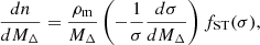 (B.1)
(B.1)
where ρm is the cosmic matter density, σ(MΔ) is the root-mean-square fluctuation of the linear density field smoothed on a scale enclosing the mass MΔ and fST is the so-called multiplicity function parameterised as
![Mathematical equation: $$ \begin{aligned} f_{\rm ST}(\sigma ) = A_{\Delta }\frac{\delta _c}{\sigma }\sqrt{\frac{2 a_{\Delta }}{\pi }}\left[1+\left(\frac{a_{\Delta }\delta _c^2}{\sigma ^2}\right)^{-p_{\Delta }}\right]e^{-\frac{a_{\Delta }\delta _c^2}{2\sigma ^2}}, \end{aligned} $$](/articles/aa/full_html/2025/05/aa53914-25/aa53914-25-eq86.gif) (B.2)
(B.2)
where AΔ, aΔ and pΔ are calibration parameters and δc is the linearly extrapolated spherical collapse threshold, which we estimate using the formula by Kitayama & Suto (1996). We derive the best-fit values of the ST coefficients at different redshifts, the corresponding best-fit ST halo mass function are shown in Fig. B.1, Fig. B.2 and Fig. B.3 respectively. We note that as we are particularly interested in the high mass regime we truncate the catalogues such that, M200 > 1013h−1 M⊙, this results in our fits being particularly ineffective at calibrating the p parameter, which we set to the value given by Despali et al. (2016).
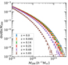 |
Fig. B.1. Halo mass function for halo masses M200 at different redshift snapshots from the UCHUU catalogues. The various lines correspond to the best-fit ST functions. |
In order to extrapolate to redshifts other than those probed by the simulation snapshots, following Despali et al. (2016) we parameterise the redshift dependence of the coefficients in terms of the variable xΔ = log10(Δ/Δvir(z)), where Δvir is the virial overdensity, which we estimate from the formula of Bryan & Norman (1998). We approximate the evolution of the ST coefficient as function of xΔ in terms of a second-order polynomial expansion:
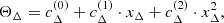 (B.3)
(B.3)
where ΘΔ = {AΔ, aΔ, pΔ}. We quote in Table B.1 the value of the best-fitting polynomial coefficients.
Best-fit coefficients of ST parameters.
Appendix C: Sparsity bias models
Here, we show the results of the Bayesian linear regression analysis of the selection-baryon sparsity bias estimates from the calibration sample discussed in Section 6.3.1 for different sparsity configurations. The bias estimates, the average linear regression fit and the 1 and 2σ credible regions are plotted in Fig. C.1.
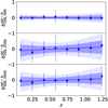 |
Fig. C.1. Estimates of the mean and standard deviation of selection-baryon bias for different sparsity configurations at different redshift bins (blue squares). The solid blue lines correspond to the average linear regression fits, while the shaded areas represents 1 and 2σ credible regions. |
The results of the Bayesian linear regression of the HE sparsity bias in the case of the X-ray and SZ calibration samples are shown in Fig. C.2.
Appendix D: Sparsity correlations
The use of sparsity mass ratios allow us to retrieve cosmological information encoded in the halo mass profile. In principle, the gravitational halo mass assembly process correlates the mass distribution across different radial shells thus leading to correlations among sparsities probing different regions of the mass profile. However, not all the sparsities are correlated to unity as one would expect if the halo density profile exactly follows the NFW profile. Indeed, as shown in Corasaniti et al. (2022), certain sparsity combinations, such as those probing distant mass shells, exhibit a low level of correlations, thus allowing to infer cosmological constraints from multiple sparsity measurements. In Corasaniti et al. (2022), the authors have evaluated the correlations among different sparsity combinations at different redshifts using the halo catalogues from large volume cosmological simulations (see their Fig. 3 and 4).
Here, we estimate the correlations among the sparsities s200, 500, s200, 2500 and s500, 2500 using the mass estimates at M200, M500 and M2500 of the simulated clusters from the DM-only, GADGET-X and GIZMO-SIMBA catalogues, as well as the HE masses from Gianfagna et al. (2023). In particular, for each sparsity pair we compute the correlation coefficient:
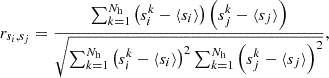 (D.1)
(D.1)
where the index i, j = {(200,500),(200,2500),(500,2500)} with i ≠ j. These are shown as function of redshift in Fig. D.1. For comparison, we also plot the correlation coefficients obtained from the halo catalogues of large volume cosmological N-body simulations such as Raygal (black solid lines) and M2CSims (black dotted lines) presented in Corasaniti et al. (2022), and the haloes from the MDPL2 simulation (black dashed line). As we can see, the correlations from the The300 simulations are very noisy. This is not surprising since they are estimated using only a few hundred clusters. Nonetheless, we can see a decreasing trend as function of redshift, consistent with the correlations from the large volume simulations.
As already pointed out in Corasaniti et al. (2022), the correlations among sparsities increase from high to low redshifts consistently with the fact that haloes grow from inside-out. As the halo mass is assembled over increasing time scales the distribution of mass within different mass shells becomes increasingly correlated. Hence, it is not surprising that such a trend remains unaltered even in the presence of baryons. We can see that sparsities such as s200, 500 and s500, 2500 probing different the mass distribution in different radial shells are less correlated than those probed by s200, 500 and s500, 2500. A larger sample of hydro simulated clusters is indeed necessary to obtain a more precise estimate of the correlations and test how they differ from those estimated from DM-only simulations.
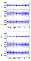 |
Fig. D.1. Estimates of the mean and standard deviation of the HE sparsity bias from the The300-X (top panel) and The300-SZ (bottom panel) calibration sample for the different sparsity configurations in different redshift bins (blue squares). The solid lines correspond to the average linear regression fits, while the shaded areas represents 1 and 2σ credible regions. |
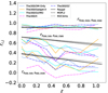 |
Fig. D.2. Correlation coefficients of the different sparsity pairs s200, 500 − s500, 2500 (lowest curves), s200, 500 − s200, 2500 (middle curves), s200, 2500 − s500, 2500 (top curves) as a function of redshifts from the DM-only (solid light-blue line), GADGET-X (solid orange line), MDPL2 (dashed red line), Raygal (solid blue line), and M2Csims (dotted green line) samples. |
All Tables
All Figures
|
Fig. 1. Normalised histograms of the sparsity s200, 500 (left panels), s200, 2500 (central panels), and s500, 2500 (right panels) obtained from the analysis of the MDPL2 sub-sample (dark blue bars) and The300/DM-only catalogue (goldenrod filled bars) at z = 0.0 (top panels), 0.5 (middle panels), and 1.0 (bottom panels), where the MDPL2 sub-sample consists of haloes with a mass larger than the minimum mass of the DM-only catalogue at the redshift considered. The vertical lines in each panel correspond to the median sparsities for the MDPL2 sub-sample (dark blue dotted line) and the The300/DM-only sample (goldenrod solid line). |
| In the text | |
|
Fig. 2. DM-only versus hydro-simulation-estimated sparsities s200, 500 (left panels), s500, 1000 (central panels) and s1000, 2500 (right panels) for the clusters in the GIZMO-SIMBA (top panels), GADGET-X (central panels), and GADGET-MUSIC (bottom panels) catalogues at z = 0, respectively. The blue squares represent clusters from the full samples, while the yellow triangles corresponds to the relaxed systems as defined in Sec. 2.2. The size of the data points is proportional to mass M200 of each cluster from the DM-only simulation. The diagonal line represents the ideal case with no bias, while the shaded areas correspond to 10% (yellow band) and 50% (light-blue band) deviation respectively. |
| In the text | |
|
Fig. 3. Sparsity relative difference Δs/s |200, Δ (top panels), Δs/s |500, Δ (central panels), and Δs/s |1000, Δ (bottom panels) as function of Δ for the GIZMO-SIMBA clusters in the catalogues at z = 0 (left panels) and 1 (right panels). The blue squares (yellow triangles) represent the average for the full (relaxed) cluster sample, while the shaded areas correspond to the standard deviation. The black dashed lines in the plots mark the 5% differences respectively, while the solid blue (yellow) lines correspond to the linear regression of the average values. |
| In the text | |
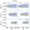 |
Fig. 4. As in Fig. 3 but for the GADGET-X catalogues. |
| In the text | |
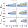 |
Fig. 5. As in Fig. 3 but for the GADGET-MUSIC catalogues. |
| In the text | |
|
Fig. 6. Average and scatter of the relative difference of the sparsity of the GADGET-X (blue squares) and GADGET-MUSIC (yellow triangles) clusters with respect to that of their GIZMO-SIMBA counterparts for different sparsity configurations in the case of the full (filled markers) and relaxed (empty markers) samples at z = 0 (top panel) and 1 (bottom panel), respectively. The errorbars represent the standard deviations for each sparsity configuration, while the shaded areas correspond to 5% and 10% variation respectively. |
| In the text | |
|
Fig. 7. Pearson’s correlation coefficients as function of redshift for the GIZMO-SIMBA (yellow markers) and GADGET-X (blue markers) clusters from the full (filled markers) and relaxed (empty markers) samples. The shaded areas (dark to light blue) correspond to “very weak”, “weak” and “moderate” correlations respectively. |
| In the text | |
|
Fig. 8. s500, 2500 versus |
| In the text | |
|
Fig. 9. Normalised histograms of the gas mass fraction ratios |
| In the text | |
|
Fig. 10. Sparsity s200, 500 estimated from the HE masses of the GADGET-X clusters from Gianfagna et al. (2023) at z = 0 (left panel), 0.5 (central panel) and 1.0 (right panel) using the X-ray temperature and gas density profiles (filled goldenrod squares) and SZ pressure profiles (empty blue circles). Values of s200, 500 ≤ 1 correspond to disturbed clusters for which the HE is not satisfied. Some of these are associated to systems with a vanishing or negative HE mass bias at R500 and a significant bias at R200. |
| In the text | |
|
Fig. 11. Probability density function of the HE sparsity bias bs200, 500 (left columns), bs200, 2500 (central columns), and bs500, 2500 (right columns) for the X-ray (blue bars) and SZ (red bars) masses, respectively, at z = 0.07 (top rows), 0.46 (central rows), and 0.99 (bottom rows). |
| In the text | |
|
Fig. 12. HE sparsity bias bs200, 500 and bs200, 2500 as function of M200 (top panels) and bs500, 2500 as function of M500 (bottom panel) for the X (left panels) and SZ (right panels) masses of the full cluster sample at z = 0.0 (blue circles), 0.5 (magenta squares), and 1.0 (green stars). The different lines correspond to the median (solid) and the mean (dashed), while the shaded area to the region comprised between the 16th and 84th percentile. |
| In the text | |
|
Fig. 13. Summary statistics of the HE sparsity bias bs200, 500 (top panels), bs200, 2500 (mid panels), and bs500, 2500 (bottom panels) as a function of redshift for the X (left panels) and SZ (right panels) masses. The different lines correspond to the median (solid) and mean (dashed), while the shaded area corresponds to the region comprised between the 16-th and 84-th percentile. |
| In the text | |
|
Fig. 14. HE sparsities sΔ1, Δ2HE from the X (blue) and SZ (red) catalogues with respect to their GADGET-X counterparts at z = 0 in the case of s200, 500 (left panel), s500, 2500(central panel), and s200, 2500 (right panel). The coloured dashed line correspond to the average linear fit to the 25 equally spaced binned data points (squares) in bins of true sparsities containing at least two clusters. The shaded areas indicates that 1 and 2σ credible regions. The black solid line corresponds to the unbiased case. |
| In the text | |
|
Fig. 15. Mean sparsities predicted by Eq. (6) with the redshift-dependent corrections (solid red lines) for the Uchuu fiducial cosmology against the estimates of the means from the UCHUU-DM data sample in equally spaced redshift bins (blue squares). |
| In the text | |
|
Fig. 16. Bayesian graph models representing the relation between the cosmological parameters (Ωm, S8), the mean sparsity model prediction at a given redshift ( |
| In the text | |
|
Fig. 17. Marginalised posterior on S8 from the analysis of single sparsity measurements for the UCHUU-DM (black curve), The300-GX (yellow curves), The300-X (blue curves) and The300-SZ (red curves). The solid lines represent posterior inferred with the simplest data model, while the dashed lines corresponds to posteriors obtained marginalising over bias model parameters. |
| In the text | |
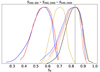 |
Fig. 18. As in Fig. 17 in the case of multiple sparsity measurements. |
| In the text | |
|
Fig. A.1. Average sparsity ⟨s200, 500⟩ as function of M200 for the clusters in the GADGET-X (top panel) and GIZMO-SIMBA (bottom panel) catalogues at z = 0 and 1, respectively. The blue solid line corresponds to the case of the full cluster sample, while the goldenrod solid line corresponds to the relaxed one. The shaded areas correspond to the standard deviation in each mass bin. |
| In the text | |
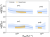 |
Fig. A.2. As in Fig. A.1 but for ⟨s500, 1000⟩ as function of M500. |
| In the text | |
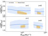 |
Fig. A.3. As in Fig. A.1 but for ⟨s1000, 2000⟩ as function of M1000c. |
| In the text | |
|
Fig. B.1. Halo mass function for halo masses M200 at different redshift snapshots from the UCHUU catalogues. The various lines correspond to the best-fit ST functions. |
| In the text | |
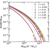 |
Fig. B.2. As in Fig. B.1 but for halo masses M500. |
| In the text | |
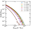 |
Fig. B.3. As in Fig. B.1 but for halo masses M2500. |
| In the text | |
|
Fig. C.1. Estimates of the mean and standard deviation of selection-baryon bias for different sparsity configurations at different redshift bins (blue squares). The solid blue lines correspond to the average linear regression fits, while the shaded areas represents 1 and 2σ credible regions. |
| In the text | |
|
Fig. D.1. Estimates of the mean and standard deviation of the HE sparsity bias from the The300-X (top panel) and The300-SZ (bottom panel) calibration sample for the different sparsity configurations in different redshift bins (blue squares). The solid lines correspond to the average linear regression fits, while the shaded areas represents 1 and 2σ credible regions. |
| In the text | |
|
Fig. D.2. Correlation coefficients of the different sparsity pairs s200, 500 − s500, 2500 (lowest curves), s200, 500 − s200, 2500 (middle curves), s200, 2500 − s500, 2500 (top curves) as a function of redshifts from the DM-only (solid light-blue line), GADGET-X (solid orange line), MDPL2 (dashed red line), Raygal (solid blue line), and M2Csims (dotted green line) samples. |
| In the text | |
Current usage metrics show cumulative count of Article Views (full-text article views including HTML views, PDF and ePub downloads, according to the available data) and Abstracts Views on Vision4Press platform.
Data correspond to usage on the plateform after 2015. The current usage metrics is available 48-96 hours after online publication and is updated daily on week days.
Initial download of the metrics may take a while.