| Issue |
A&A
Volume 684, April 2024
|
|
|---|---|---|
| Article Number | A139 | |
| Number of page(s) | 19 | |
| Section | Cosmology (including clusters of galaxies) | |
| DOI | https://doi.org/10.1051/0004-6361/202348743 | |
| Published online | 17 April 2024 | |
Euclid preparation
XXXVII. Galaxy colour selections with Euclid and ground photometry for cluster weak-lensing analyses
1
Dipartimento di Fisica e Astronomia “Augusto Righi” – Alma Mater Studiorum Università di Bologna, Via Piero Gobetti 93/2, 40129 Bologna, Italy
e-mail: This email address is being protected from spambots. You need JavaScript enabled to view it.
2
INAF-Osservatorio di Astrofisica e Scienza dello Spazio di Bologna, Via Piero Gobetti 93/3, 40129 Bologna, Italy
3
INFN-Sezione di Bologna, Viale Berti Pichat 6/2, 40127 Bologna, Italy
4
INAF-Osservatorio Astronomico di Padova, Via dell’Osservatorio 5, 35122 Padova, Italy
5
Dipartimento di Fisica e Astronomia “G. Galilei”, Università di Padova, Via Marzolo 8, 35131 Padova, Italy
6
Université Paris-Saclay, Université Paris Cité, CEA, CNRS, AIM, 91191 Gif-sur-Yvette, France
7
Department of Physics “E. Pancini”, University Federico II, Via Cinthia 6, 80126 Napoli, Italy
8
INAF-Osservatorio Astronomico di Capodimonte, Via Moiariello 16, 80131 Napoli, Italy
9
INFN Section of Naples, Via Cinthia 6, 80126 Napoli, Italy
10
Istituto Nazionale di Fisica Nucleare, Sezione di Bologna, Via Irnerio 46, 40126 Bologna, Italy
11
Université Côte d’Azur, Observatoire de la Côte d’Azur, CNRS, Laboratoire Lagrange, Bd de l’Observatoire, CS 34229, 06304 Nice Cedex 4, France
12
INAF-Osservatorio Astronomico di Trieste, Via G. B. Tiepolo 11, 34143 Trieste, Italy
13
IFPU, Institute for Fundamental Physics of the Universe, Via Beirut 2, 34151 Trieste, Italy
14
Université Paris-Saclay, CNRS, Institut d’Astrophysique Spatiale, 91405 Orsay, France
15
Institute of Cosmology and Gravitation, University of Portsmouth, Portsmouth PO1 3FX, UK
16
INAF-Osservatorio Astronomico di Brera, Via Brera 28, 20122 Milano, Italy
17
Dipartimento di Fisica e Astronomia, Università di Bologna, Via Gobetti 93/2, 40129 Bologna, Italy
18
Max Planck Institute for Extraterrestrial Physics, Giessenbachstr. 1, 85748 Garching, Germany
19
Universitäts-Sternwarte München, Fakultät für Physik, Ludwig-Maximilians-Universität München, Scheinerstrasse 1, 81679 München, Germany
20
INAF-Osservatorio Astrofisico di Torino, Via Osservatorio 20, 10025 Pino Torinese, TO, Italy
21
Dipartimento di Fisica, Università di Genova, Via Dodecaneso 33, 16146 Genova, Italy
22
INFN-Sezione di Genova, Via Dodecaneso 33, 16146 Genova, Italy
23
Instituto de Astrofísica e Ciências do Espaço, Universidade do Porto, CAUP, Rua das Estrelas, 4150-762 Porto, Portugal
24
Dipartimento di Fisica, Università degli Studi di Torino, Via P. Giuria 1, 10125 Torino, Italy
25
INFN-Sezione di Torino, Via P. Giuria 1, 10125 Torino, Italy
26
INAF-IASF Milano, Via Alfonso Corti 12, 20133 Milano, Italy
27
Institut de Física d’Altes Energies (IFAE), The Barcelona Institute of Science and Technology, Campus UAB, 08193 Bellaterra, Barcelona, Spain
28
Port d’Informació Científica, Campus UAB, C. Albareda s/n, 08193 Bellaterra, Barcelona, Spain
29
Institute for Theoretical Particle Physics and Cosmology (TTK), RWTH Aachen University, 52056 Aachen, Germany
30
Institute of Space Sciences (ICE, CSIC), Campus UAB, Carrer de Can Magrans, s/n, 08193 Barcelona, Spain
31
Institut d’Estudis Espacials de Catalunya (IEEC), Carrer Gran Capitá 2-4, 08034 Barcelona, Spain
32
INAF-Osservatorio Astronomico di Roma, Via Frascati 33, 00078 Monteporzio Catone, Italy
33
Dipartimento di Fisica e Astronomia “Augusto Righi” – Alma Mater Studiorum Università di Bologna, Viale Berti Pichat 6/2, 40127 Bologna, Italy
34
Institute for Astronomy, University of Edinburgh, Royal Observatory, Blackford Hill, Edinburgh EH9 3HJ, UK
35
Jodrell Bank Centre for Astrophysics, Department of Physics and Astronomy, University of Manchester, Oxford Road, Manchester M13 9PL, UK
36
European Space Agency/ESRIN, Largo Galileo Galilei 1, 00044 Frascati, Roma, Italy
37
ESAC/ESA, Camino Bajo del Castillo, s/n, Urb. Villafranca del Castillo, 28692 Villanueva de la Cañada, Madrid, Spain
38
University of Lyon, Univ. Claude Bernard Lyon 1, CNRS/IN2P3, IP2I Lyon, UMR 5822, 69622 Villeurbanne, France
39
Institute of Physics, Laboratory of Astrophysics, Ecole Polytechnique Fédérale de Lausanne (EPFL), Observatoire de Sauverny, 1290 Versoix, Switzerland
40
UCB Lyon 1, CNRS/IN2P3, IUF, IP2I Lyon, 4 Rue Enrico Fermi, 69622 Villeurbanne, France
41
Departamento de Física, Faculdade de Ciências, Universidade de Lisboa, Edifício C8, Campo Grande, 1749-016 Lisboa, Portugal
42
Instituto de Astrofísica e Ciências do Espaço, Faculdade de Ciências, Universidade de Lisboa, Campo Grande, 1749-016 Lisboa, Portugal
43
Department of Astronomy, University of Geneva, Ch. d’Ecogia 16, 1290 Versoix, Switzerland
44
INAF-Istituto di Astrofisica e Planetologia Spaziali, Via del Fosso del Cavaliere, 100, 00100 Roma, Italy
45
Department of Physics, Oxford University, Keble Road, Oxford OX1 3RH, UK
46
INFN-Padova, Via Marzolo 8, 35131 Padova, Italy
47
Institut de Ciencies de l’Espai (IEEC-CSIC), Campus UAB, Carrer de Can Magrans, s/n Cerdanyola del Vallés, 08193 Barcelona, Spain
48
School of Physics, HH Wills Physics Laboratory, University of Bristol, Tyndall Avenue, Bristol BS8 1TL, UK
49
University Observatory, Faculty of Physics, Ludwig-Maximilians-Universität, Scheinerstr. 1, 81679 Munich, Germany
50
Institute of Theoretical Astrophysics, University of Oslo, PO Box 1029 Blindern, 0315 Oslo, Norway
51
Department of Physics, Lancaster University, Lancaster LA1 4YB, UK
52
von Hoerner & Sulger GmbH, SchloßPlatz 8, 68723 Schwetzingen, Germany
53
Technical University of Denmark, Elektrovej 327, 2800 Kgs. Lyngby, Denmark
54
Cosmic Dawn Center (DAWN), Copenhagen, Denmark
55
Institut d’Astrophysique de Paris, UMR 7095, CNRS, and Sorbonne Université, 98 bis boulevard Arago, 75014 Paris, France
56
Max-Planck-Institut für Astronomie, Königstuhl 17, 69117 Heidelberg, Germany
57
Aix-Marseille Université, CNRS/IN2P3, CPPM, Marseille, France
58
Jet Propulsion Laboratory, California Institute of Technology, 4800 Oak Grove Drive, Pasadena, CA 91109, USA
59
AIM, CEA, CNRS, Université Paris-Saclay, Université de Paris, 91191 Gif-sur-Yvette, France
60
Université de Genève, Département de Physique Théorique and Centre for Astroparticle Physics, 24 Quai Ernest-Ansermet, 1211 Genève 4, Switzerland
61
Department of Physics, University of Helsinki, PO Box 64 00014 Helsinki, Finland
62
Helsinki Institute of Physics, University of Helsinki, Gustaf Hällströmin katu 2, Helsinki, Finland
63
NOVA Optical Infrared Instrumentation Group at ASTRON, Oude Hoogeveensedijk 4, 7991 PD Dwingeloo, The Netherlands
64
Universität Bonn, Argelander-Institut für Astronomie, Auf dem Hügel 71, 53121 Bonn, Germany
65
Aix-Marseille Université, CNRS, CNES, LAM, Marseille, France
66
Department of Physics, Institute for Computational Cosmology, Durham University, South Road, DH1 3LE Durham, UK
67
University of Applied Sciences and Arts of Northwestern Switzerland, School of Engineering, 5210 Windisch, Switzerland
68
Institut d’Astrophysique de Paris, 98bis Boulevard Arago, 75014 Paris, France
69
European Space Agency/ESTEC, Keplerlaan 1, 2201 AZ Noordwijk, The Netherlands
70
Department of Physics and Astronomy, University of Aarhus, Ny Munkegade 120, 8000 Aarhus C, Denmark
71
Université Paris-Saclay, Université Paris Cité, CEA, CNRS, Astrophysique, Instrumentation et Modélisation Paris-Saclay, 91191 Gif-sur-Yvette, France
72
Space Science Data Center, Italian Space Agency, Via del Politecnico snc, 00133 Roma, Italy
73
Centre National d’Etudes Spatiales – Centre Spatial de Toulouse, 18 Avenue Edouard Belin, 31401 Toulouse Cedex 9, France
74
Institute of Space Science, Str. Atomistilor, nr. 409 Măgurele, Ilfov 077125, Romania
75
Instituto de Astrofísica de Canarias, Calle Vía Láctea s/n, 38204 San Cristóbal de La Laguna, Tenerife, Spain
76
Departamento de Astrofísica, Universidad de La Laguna, 38206 La Laguna, Tenerife, Spain
77
Departamento de Física, FCFM, Universidad de Chile, Blanco Encalada, 2008 Santiago, Chile
78
Satlantis, University Science Park, Sede Bld, 48940 Leioa-Bilbao, Spain
79
Centre for Electronic Imaging, Open University, Walton Hall, Milton Keynes MK7 6AA, UK
80
Centro de Investigaciones Energéticas, Medioambientales y Tecnológicas (CIEMAT), Avenida Complutense 40, 28040 Madrid, Spain
81
Infrared Processing and Analysis Center, California Institute of Technology, Pasadena, CA 91125, USA
82
Instituto de Astrofísica e Ciências do Espaço, Faculdade de Ciências, Universidade de Lisboa, Tapada da Ajuda, 1349-018 Lisboa, Portugal
83
Universidad Politécnica de Cartagena, Departamento de Electrónica y Tecnología de Computadoras, Plaza del Hospital 1, 30202 Cartagena, Spain
84
Institut de Recherche en Astrophysique et Planétologie (IRAP), Université de Toulouse, CNRS, UPS, CNES, 14 Av. Edouard Belin, 31400 Toulouse, France
85
Kapteyn Astronomical Institute, University of Groningen, PO Box 800 9700 AV Groningen, The Netherlands
86
INFN-Bologna, Via Irnerio 46, 40126 Bologna, Italy
87
Department of Mathematics and Physics E. De Giorgi, University of Salento, Via per Arnesano, CP-I93, 73100 Lecce, Italy
88
INAF-Sezione di Lecce, c/o Dipartimento Matematica e Fisica, Via per Arnesano, 73100 Lecce, Italy
89
INFN, Sezione di Lecce, Via per Arnesano, CP-193, 73100 Lecce, Italy
90
Institut für Theoretische Physik, University of Heidelberg, Philosophenweg 16, 69120 Heidelberg, Germany
91
Université St Joseph; Faculty of Sciences, Beirut, Lebanon
92
Junia, EPA department, 41 Bd Vauban, 59800 Lille, France
93
SISSA, International School for Advanced Studies, Via Bonomea 265, 34136 Trieste, TS, Italy
94
INFN, Sezione di Trieste, Via Valerio 2, 34127 Trieste, TS, Italy
95
ICSC – Centro Nazionale di Ricerca in High Performance Computing, Big Data e Quantum Computing, Via Magnanelli 2, Bologna, Italy
96
Instituto de Física Teórica UAM-CSIC, Campus de Cantoblanco, 28049 Madrid, Spain
97
CERCA/ISO, Department of Physics, Case Western Reserve University, 10900 Euclid Avenue, Cleveland, OH 44106, USA
98
Laboratoire Univers et Théorie, Observatoire de Paris, Université PSL, Université Paris Cité, CNRS, 92190 Meudon, France
99
Dipartimento di Fisica e Scienze della Terra, Università degli Studi di Ferrara, Via Giuseppe Saragat 1, 44122 Ferrara, Italy
100
Istituto Nazionale di Fisica Nucleare, Sezione di Ferrara, Via Giuseppe Saragat 1, 44122 Ferrara, Italy
101
Dipartimento di Fisica – Sezione di Astronomia, Università di Trieste, Via Tiepolo 11, 34131 Trieste, Italy
102
NASA Ames Research Center, Moffett Field, CA 94035, USA
103
Kavli Institute for Particle Astrophysics & Cosmology (KIPAC), Stanford University, Stanford, CA 94305, USA
104
Bay Area Environmental Research Institute, Moffett Field, CA 94035, USA
105
Minnesota Institute for Astrophysics, University of Minnesota, 116 Church St SE, Minneapolis, MN 55455, USA
106
INAF, Istituto di Radioastronomia, Via Piero Gobetti 101, 40129 Bologna, Italy
107
Institute Lorentz, Leiden University, PO Box 9506 Leiden 2300 RA, The Netherlands
108
Institute for Astronomy, University of Hawaii, 2680 Woodlawn Drive, Honolulu, HI 96822, USA
109
Department of Physics & Astronomy, University of California Irvine, Irvine, CA 92697, USA
110
Department of Astronomy & Physics and Institute for Computational Astrophysics, Saint Mary’s University, 923 Robie Street, Halifax, Nova Scotia B3H 3C3, Canada
111
Departamento Física Aplicada, Universidad Politécnica de Cartagena, Campus Muralla del Mar, 30202 Cartagena, Murcia, Spain
112
Université Paris Cité, CNRS, Astroparticule et Cosmologie, 75013 Paris, France
113
Department of Computer Science, Aalto University, PO Box 15400 Espoo 00 076, Finland
114
NRC Herzberg, 5071 West Saanich Rd, Victoria, BC V9E 2E7, Canada
115
Ruhr University Bochum, Faculty of Physics and Astronomy, Astronomical Institute (AIRUB), German Centre for Cosmological Lensing (GCCL), 44780 Bochum, Germany
116
Instituto de Astrofísica de Canarias (IAC), Departamento de Astrofísica, Universidad de La Laguna (ULL), 38200 La Laguna, Tenerife, Spain
117
Université PSL, Observatoire de Paris, Sorbonne Université, CNRS, LERMA, 75014 Paris, France
118
Université Paris-Cité, 5 Rue Thomas Mann, 75013 Paris, France
119
Univ. Grenoble Alpes, CNRS, Grenoble INP, LPSC-IN2P3, 53, Avenue des Martyrs, 38000 Grenoble, France
120
Department of Physics and Astronomy, University of Turku, Vesilinnantie 5, 20014 Turku, Finland
121
Serco for European Space Agency (ESA), Camino bajo del Castillo, s/n, Urbanizacion Villafranca del Castillo, Villanueva de la Cañada, 28692 Madrid, Spain
122
Centre for Astrophysics & Supercomputing, Swinburne University of Technology, Victoria 3122, Australia
123
ARC Centre of Excellence for Dark Matter Particle Physics, Melbourne, Australia
124
Department of Physics and Helsinki Institute of Physics, University of Helsinki, Gustaf Hällströmin katu 2, 00014 Helsinki, Finland
125
Oskar Klein Centre for Cosmoparticle Physics, Department of Physics, Stockholm University, Stockholm 106 91, Sweden
126
Astrophysics Group, Blackett Laboratory, Imperial College London, London SW7 2AZ, UK
127
Centre de Calcul de l’IN2P3/CNRS, 21 Avenue Pierre de Coubertin, 69627 Villeurbanne Cedex, France
128
Dipartimento di Fisica, Sapienza Università di Roma, Piazzale Aldo Moro 2, 00185 Roma, Italy
129
INFN-Sezione di Roma, Piazzale Aldo Moro 2 – c/o Dipartimento di Fisica, Edificio G. Marconi, 00185 Roma, Italy
130
Centro de Astrofísica da Universidade do Porto, Rua das Estrelas, 4150-762 Porto, Portugal
131
Zentrum für Astronomie, Universität Heidelberg, Philosophenweg 12, 69120 Heidelberg, Germany
132
Dipartimento di Fisica, Università di Roma Tor Vergata, Via della Ricerca Scientifica 1, Roma, Italy
133
INFN, Sezione di Roma 2, Via della Ricerca Scientifica 1, Roma, Italy
134
Institute for Computational Science, University of Zurich, Winterthurerstrasse 190, 8057 Zurich, Switzerland
135
Mullard Space Science Laboratory, University College London, Holmbury St Mary, Dorking, Surrey RH5 6NT, UK
136
Department of Physics and Astronomy, University of California, Davis, CA 95616, USA
137
Department of Astrophysical Sciences, Peyton Hall, Princeton University, Princeton, NJ 08544, USA
138
Niels Bohr Institute, University of Copenhagen, Jagtvej 128, 2200 Copenhagen, Denmark
Received:
27
November
2023
Accepted:
19
January
2024
Abstract
Aims. We derived galaxy colour selections from Euclid and ground-based photometry, aiming to accurately define background galaxy samples in cluster weak-lensing analyses. These selections have been implemented in the Euclid data analysis pipelines for galaxy clusters.
Methods. Given any set of photometric bands, we developed a method for the calibration of optimal galaxy colour selections that maximises the selection completeness, given a threshold on purity. Such colour selections are expressed as a function of the lens redshift.
Results. We calibrated galaxy selections using simulated ground-based griz and EuclidYEJEHE photometry. Both selections produce a purity higher than 97%. The griz selection completeness ranges from 30% to 84% in the lens redshift range zl ∈ [0.2, 0.8]. With the full grizYEJEHE selection, the completeness improves by up to 25 percentage points, and the zl range extends up to zl = 1.5. The calibrated colour selections are stable to changes in the sample limiting magnitudes and redshift, and the selection based on griz bands provides excellent results on real external datasets. Furthermore, the calibrated selections provide stable results using alternative photometric aperture definitions obtained from different ground-based telescopes. The griz selection is also purer at high redshift and more complete at low redshift compared to colour selections found in the literature. We find excellent agreement in terms of purity and completeness between the analysis of an independent, simulated Euclid galaxy catalogue and our calibration sample, except for galaxies at high redshifts, for which we obtain up to 50 percentage points higher completeness. The combination of colour and photo-z selections applied to simulated Euclid data yields up to 95% completeness, while the purity decreases down to 92% at high zl. We show that the calibrated colour selections provide robust results even when observations from a single band are missing from the ground-based data. Finally, we show that colour selections do not disrupt the shear calibration for stage III surveys. The first Euclid data releases will provide further insights into the impact of background selections on the shear calibration.
Key words: galaxies: clusters: general / galaxies: distances and redshifts / galaxies: photometry / galaxies: statistics / cosmology: observations / large-scale structure of Universe
© The Authors 2024
 Open Access article, published by EDP Sciences, under the terms of the Creative Commons Attribution License (https://creativecommons.org/licenses/by/4.0), which permits unrestricted use, distribution, and reproduction in any medium, provided the original work is properly cited.
This article is published in open access under the Subscribe to Open model. This email address is being protected from spambots. You need JavaScript enabled to view it. to support open access publication.
1. Introduction
In the last decade, galaxy clusters have proven to be excellent probes for cosmological analyses (see, e.g. Mantz et al. 2015; Sereno et al. 2015; Planck Collaboration XXIV 2016; Costanzi et al. 2019; Marulli et al. 2021; Lesci et al. 2022), also allowing for the investigation of dark matter interaction models (Peter et al. 2013; Robertson et al. 2017; Eckert et al. 2022) and gas astrophysics (Vazza et al. 2017; CHEX-MATE Collaboration 2021; Zhu et al. 2021; Sereno et al. 2021). As galaxy clusters are dominated by dark matter, the functional form of their matter density profiles can be derived from N-body dark-matter-only simulations (Navarro et al. 1997; Baltz et al. 2009; Diemer & Kravtsov 2014). This allows one to estimate the mass of observed clusters, which is essential for both astrophysical and cosmological studies (Teyssier et al. 2011; Pratt et al. 2019). Currently, weak gravitational lensing is one of the most reliable methods to accurately and precisely measure cluster masses (Okabe et al. 2010; Hoekstra et al. 2012; Melchior et al. 2015; Sereno et al. 2017; Stern et al. 2019; Schrabback et al. 2021; Zohren et al. 2022). Consequently, weak-lensing cluster mass estimates are widely used in current photometric galaxy surveys, such as the Kilo Degree Survey (KiDS; Kuijken et al. 2019; Bellagamba et al. 2019), the Dark Energy Survey (DES; Abbott et al. 2020; Sevilla-Noarbe et al. 2021), and the Hyper Suprime-Cam survey (HSC; Medezinski et al. 2018; Li et al. 2022).
An accurate selection of lensed background galaxies is crucial to derive a reliable cluster weak-lensing signal. Including the contribution from foreground and cluster member galaxies may significantly dilute the weak-lensing signal (Broadhurst et al. 2005; Medezinski et al. 2007; Sifón et al. 2015; McClintock et al. 2019). For example, background selections with 90% purity dilute the cluster reduced shear measurements by 10% (see, e.g. Dietrich et al. 2019), in the absence of intrinsic alignments (Heymans & Heavens 2003). Highly pure background selections are required to properly account for this effect in weak-lensing measurements, in order to minimise the variance in the selection purity. Selection incompleteness, instead, impacts the weak-lensing noise and, in turn, the signal-to-noise ratio (S/N), which depends on the density of background sources along with the intrinsic ellipticity dispersion and measurement noise (see, e.g. Schrabback et al. 2018; Umetsu 2020). The effect of low background densities can be partially mitigated by increasing the size of the cluster-centric radial bins used in the analysis, or through the stacking of the weak-lensing signal of cluster ensembles.
Background selections based on the galaxy photometric redshift (photo-z) posteriors are commonly used in the literature (Gruen et al. 2014; Applegate et al. 2014; Melchior et al. 2017; Sereno et al. 2017; Bellagamba et al. 2019), as well as galaxy colour selections (Medezinski et al. 2010, 2018; Oguri et al. 2012; Klein et al. 2019). These selections can also be combined to significantly improve the background sample completeness and, in turn, the weak-lensing S/N. In fact, colour selections have been demonstrated to help identify galaxies with poorly defined photometric redshifts that would not have been classified as background sources through photo-z selection alone (Covone et al. 2014; Sereno et al. 2017; Bellagamba et al. 2019).
The aim of this paper is to develop a method to obtain optimal colour selections, namely with a maximal completeness given a threshold on purity, given any set of photometric filters. We provide, for the first time, colour selections expressed as a continuous function of the lens limiting redshift. This allows for a finer background definition compared to colour selections found in the literature (Medezinski et al. 2010, 2018; Oguri et al. 2012), implying a significant improvement in the weak-lensing source statistics. In view of Euclid and stage IV surveys, we derived colour selections on simulated data. We exploited the galaxy catalogue developed by Bisigello et al. (2020, hereafter referred to as B20), and extended by Euclid Collaboration (2023a), which includes simulated Sloan Digital Sky Survey (SDSS; Gunn et al. 1998) griz magnitudes and simulated Euclid observations in the YEJEHE bands. In addition, we tested the efficiency of these colour selections on real public external data and on simulations, combining them with photo-z selections.
This paper is part of a series presenting and discussing mass measurements of galaxy clusters using the Euclid combined clusters and weak-lensing pipeline COMB-CL. COMB-CL forms part of the global Euclid data processing pipeline and is responsible for measuring weak-lensing shear profiles and masses for photometrically detected clusters. A comprehensive description of the code structure and methods employed by COMB-CL will be presented in a forthcoming paper, but a brief overview of the pipeline can be found in the appendix of Euclid Collaboration (2023b). The galaxy colour selections presented in this paper are already implemented in COMB-CL.
The paper is organised as follows. In Sect. 2, we describe the dataset used for the calibration of galaxy colour selections, and in Sect. 3 we detail a general method to derive optimal colour selections. In Sect. 4, we show the selections obtained for griz and grizYEJEHE filter sets, validating them on external datasets. In Sect. 5 we compare the griz selection calibrated in this work with selections from the literature. Finally, in Sect. 6, we draw our conclusions.
2. Calibration sample
We based our analysis on the photometric catalogue developed by B20 and extended by Euclid Collaboration (2023a). This catalogue contains simulated EuclidIEYEJEHE aperture magnitudes1, covering the spectral range 5500−20 000 Å, along with the Canada-France Imaging Survey (CFIS; Ibata et al. 2017) u band, for the galaxies contained in the COSMOS catalogue by Laigle et al. (2016, COSMOS15). Specifically, such photometry is based on 3″ fixed-aperture magnitudes. Despite the u band already being present in COSMOS15, B20 derived it using the same approach adopted for the other filters in order to avoid colour biases. B20 verified that this provides results that are consistent with the observed fluxes. Simulated SDSS griz magnitudes, spanning the wavelength range 4000−11 000 Å, are also provided in the catalogue, since observations in similar filters, such as those in Vera C. Rubin Observatory (Rubin/LSST; Ivezic et al. 2008) and DES, will be available to complement Euclid observations (Euclid Collaboration 2021, 2022a). Corrections for photometric offsets due to flux outside the fixed-aperture, systematic offsets, and Galactic extinction, as suggested in Laigle et al. (2016), have been applied. B20 derive simulated magnitudes through two alternative approaches. The first is a linear interpolation of the 30 medium-band and broad-band filters available in the COSMOS15 catalogue, based on the effective wavelength of the filters. The second approach is based on the best theoretical template that describes the spectral energy distribution (SED) of each galaxy, assuming the COSMOS15 redshifts as the ground truth. The SED fitting is performed based on COSMOS15 bands and the template resulting in the minimum χ2 is used to predict the expected fluxes. We refer to B20 for the details of the SED templates used, based on the model by Bruzual & Charlot (2003). The expected fluxes are then randomised 10 times considering a Gaussian distribution centred on the true flux and with standard deviation equal to the expected photometric uncertainities, scaled considering the depths listed in Table 1 of Euclid Collaboration (2023a). In this process, the IEYEJEHE magnitude errors expected for the Euclid Wide Survey are considered. Despite the fact that the griz photometry is based on SDSS filter transmissions, the corresponding uncertainties are based on depths that are consistent with those of DES and the Ultraviolet Near-Infrared Optical Northern Survey (UNIONS)2. The ugriz photometry provided by LSST is expected to go from 1 to 2.5 mag deeper at the end of the Euclid mission, depending on the photometric filter. Throughout this paper, we focus on the magnitudes derived from the best theoretical SED templates, as these estimates better reproduce absorption and emission lines that are not covered by COSMOS15 bands. We neglect u magnitudes since, due to the low u-band throughput, a 5σ depth of 25.6 mag will only be reached after 10 years of LSST observations3. In addition, the u band is not available in DES wide fields. We emphasise that the B20 catalogue contains all the galaxies present in the COSMOS15 sample, which is deeper than the shear samples derived from current surveys (see, e.g. Giblin et al. 2021; Gatti et al. 2021) and expected from the Euclid Wide Survey (Euclid Collaboration 2022a). As we discuss in the following, the colour selections calibrated in this study yield robust results against alternative magnitude cuts, including those that reproduce the selections adopted in current and Euclid cosmic shear analyses.
3. Method
In order to find a set of optimal galaxy colour-redshift relations that maximises the selection completeness given a threshold on the foreground contamination, we considered the colours given by any combination of photometric bands. This includes bands that are not adjacent in wavelength. Thus, for each colour-colour space, given a redshift lower limit, zl, corresponding to the lens redshift, we considered the following set of conditions,
 (1)
(1)
where ∨ is the logical “or” operator, x and y are two different colours, and ci and si are colour selection parameters. Specifically, c1, …, c8 ∈ ( − ∞, +∞), s1 and s3 ∈ (0, +∞), while s2 and s4 ∈ ( − ∞, 0). The edges of the aforementioned parameter ranges are excluded, and Eq. (1) defines an irregular octagon that contains the foreground galaxies, as we show in Fig. 1. As we shall see, since we only select the colour conditions that satisfy given requirements, not all the sides of the irregular octagon may be considered. In addition, since we considered the conditions in Eq. (1) as independent, the c1, …, c8 and s1, …, s4 parameters are not related to each other. In particular, for each condition in Eq. (1), we derived the completeness,
 (2)
(2)
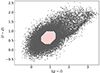 |
Fig. 1. Example of an uncalibrated selection in the (r − z)−(g − i) colour-colour space. The grey dots represent the selected galaxy colours. Galaxies within the octagonal hatched region are excluded by applying Eq. (1). Specifically, (r − z) and (g − i) correspond to x and y in Eq. (1), respectively. |
and the purity,
 (3)
(3)
where i is the ith colour condition index, zg is the galaxy redshift, p is the set of colour condition parameters, Nsel, i is the number of galaxies selected with the ith colour condition, Ntot is the total number of galaxies in the calibration sample, while the nf superscript represents quantities derived from colour conditions not fitted as a function of zl. As we shall see, we do not adopt any superscripts for the quantities derived from fitted colour conditions. In Eqs. (2) and (3), we have i = 1… Ncond, where Ncond is the number of all possible colour conditions, given Eq. (1), expressed as
 (4)
(4)
where Ncol is the number of colours, given by
 (5)
(5)
where Nband is the number of photometric bands.
We set requirements on completeness and purity to be satisfied by each colour condition in Eq. (1). Specifically, for a given zl, we selected the colour conditions having at least one p set providing  and
and  larger than their corresponding thresholds. We remark that p does not explicitly depend on zl at this stage, and that zl values are arbitrarily sampled. Setting a threshold on
  is important for excluding colour conditions that do not significantly contribute to the total completeness, and that may appear as optimal only due to statistical fluctuations. Thus, the threshold on
  is meant to be low compared to that on
  . Indeed, as we shall detail in Sect. 4.6, impurities in the background selection imply systematic uncertainties in galaxy cluster reduced shear measurements. Highly pure selections are required to properly account for this effect, in order to minimise the scatter in purity. We discuss the choice of the thresholds on
  and
and  in greater detail in Sect. 4.1. For each colour condition in Eq. (1), with parameter values for which the conditions on
  and
and  are satisfied, we selected the p set providing the highest completeness at a given zl. In this way, we derived the set of optimal colour conditions maximising the selection completeness, given the chosen threshold on purity.
We note that the maximum zl of the calibrated colour selections depends on the  and
and  limits, while the minimum zl is derived by excluding the zl points for which
  . Here,
  and
and  are the completeness and the foreground failure rate given by the full set of optimal colour conditions, respectively. For simplicity, we drop the dependence on p in the text. The foreground failure rate is defined as follows:
 (6)
(6)
where Nsel is the number of galaxies selected with all the optimal colour conditions, given a condition on zg, and  is the purity given by the full set of optimal conditions. On the right-hand side of Eq. (6), derived from Eqs. (2) and (3), we can see that
  diminishes with increasing zl if high lower limits on purity are chosen. We stress that
  by definition.
In the selection process described above, some colour conditions may be redundant. Thus, we iteratively searched for an optimal subset of colour conditions to find the minimum number of conditions sufficient to approximately reproduce the required completeness. Specifically, at each step of this iterative process, we computed the following quantity:
 (7)
(7)
where N is the number of zl points,  is the completeness given by all optimal conditions, while 𝒞nf(zl, j) is the completeness given by a subset of optimal conditions, computed at the jth zl value. As the first step of this iterative process, we found the optimal colour condition minimising 𝒮nf. Then, at each iteration, we added the colour condition that, combined with the conditions selected in the previous steps, minimises 𝒮nf. We repeated this process until 𝒮nf was lower than a given tolerance. We remark that the logical operator between colour conditions is ∨.
Lastly, we applied a nonlinear least squares analysis to find the best fit to the p parameters as a function of zl for the subset of optimal colour conditions. We chose the fitting formulae which best reproduce the zl dependence, namely polynomials, while aiming at minimising the number of free parameters in the fit.
In Fig. 2 we show a flowchart summarising the calibration process described in this section. In Fig. 3 we show an example of the iterative process detailed above, while Fig. 4 displays an example of parameter dependence on zl. Hereafter, we refer to the completeness, purity, and foreground failure rate, derived from sets of fitted colour conditions, as 𝒞(zl), 𝒫(zl), and ℱ(zl), respectively. For better clarity, in Table 1 we summarise the symbols referring to the completeness functions introduced in this section.
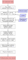 |
Fig. 2. Flowchart summarising the calibration process described in Sect. 3. Round red rectangles represent the start and end points of the calibration process. Grey rectangles represent processing steps, while blue trapezoids correspond to the inputs. |
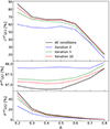 |
Fig. 3. Selection completeness (top panel), purity (middle panel), and foreground failure rate (bottom panel), derived from subsets of optimal colour conditions not fitted as a function of zl, for the case of griz photometry. The solid black lines represent the selection given by the full set of optimal colour conditions, while the dashed lines show the selection at different steps of the iterative process detailed in Sect. 3, given by subsets of optimal conditions. |
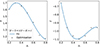 |
Fig. 4. Values of s (left panel) and c (right panel) parameters, from Eq. (1), as a function of zl for the colour condition quoted in the left panel legend. The black dots represent the optimal values of s and c, while the blue curves represent the polynomial fits. |
4. Results
4.1. Calibration of colour selections
By applying the methods detailed in Sect. 3 and adopting the B20 calibration sample described in Sect. 2, we calibrated galaxy colour selections using ground-based and Euclid photometry, namely SDSS griz and EuclidYEJEHE filters, respectively. These selections are implemented in COMB-CL, and will be available for weak-lensing analyses of galaxy clusters. We considered the following cases: ground-only, Euclid-only, and the combination of ground-based and Euclid photometry. For the cases including Euclid photometry, we adopted an S/N threshold for Euclid near-infrared observations of (S/N)E > 3, which corresponds to YE < 24.85, JE < 25.05, and HE < 24.95 (Euclid Collaboration 2022a). In addition, we considered zl points in the range zl ∈ [0.1, 2.5], assuming a precision of δzl = 0.1 for the sampling. To derive the full set of optimal colour conditions, we imposed  > 10% for the ith colour condition. For the ground-only and Euclid-only cases, we imposed that the purity of each colour condition is
  > 99%. We adopted a more restrictive threshold on purity for the combination of ground-based and Euclid photometry, corresponding to
  > 99.7%. This threshold is chosen as the larger number of colour combinations leads to a higher summation of impurities. We obtained 𝒫nf(zl) > 97% for any zl, when combining all the optimal colour conditions, as shown in Fig. 5. As we shall discuss in Sect. 4.3, the purity derived from different real datasets is stable, showing sub-percent changes, on average.
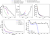 |
Fig. 5. Summary of the results on the colour selection optimisation, based on the B20 galaxy sample. Top panels: selection completeness (left panel), purity (central panel), and foreground failure rate (right panel), as a function of zl. The dashed lines represent the selections derived from the full sets of optimal conditions not fitted as a function of zl, in the case of ground-only (red), Euclid-only (green), and the combination of ground-based and Euclid bands (grey). The solid lines represent the selections obtained from the subsets of optimal conditions, with parameters fitted as a function of zl, in the case of ground-only (blue) and for the combination of ground-based and Euclid bands (black). Bottom panels: in the left panel, 𝒮 and 𝒮nf are shown as a function of the iteration number. For the ground-based selection, using griz filters, 𝒮 and 𝒮nf are represented by solid blue and dashed red lines, respectively. For the selection derived from the combination of ground-based and Euclid filters, namely grizYEJEHE, 𝒮 and 𝒮nf are represented by solid black and dashed grey lines, respectively. In the right panel, the difference between |

The ℱnf(zl) decrease with increasing zl, shown in Fig. 5, is expected, as discussed in Sect. 3. In addition, for any combination of photometric bands, we found  for zl = 0.1. Consequently, we set zl = 0.2 as the minimum lens redshift for the calibrated colour selections. As shown in Fig. 5, from griz photometry we derived a selection within zl ∈ [0.2, 0.8], with 84% completeness at zl = 0.2, decreasing to 29% at zl = 0.8. In the Euclid-only case, namely YEJEHE and IE bands, results are not competitive with those derived from griz photometry. On the other hand, by combining ground-based and Euclid photometry, the completeness significantly increases in the zl range covered by the griz selection, by up to 25 percentage points. Also the zl range of the selection is significantly extended compared to the griz case, corresponding to zl ∈ [0.2, 1.5]. Specifically, in this case we exclude the EuclidIE band, as it covers a large wavelength interval, namely ∼5000−10 000 Å, corresponding to the wavelength range already covered by griz photometry. Furthermore, the use of very broad photometric bands is not the most optimal choice for calibrating galaxy colour selections, which share similarities with photo-z estimates.
We excluded any possible redundant colour condition, as detailed in Sect. 3. In Table A.1 we show the subset of optimal colour conditions for the ground-only case, namely griz photometry, along with the corresponding parameter fits. The first condition quoted in Table A.1 corresponds to the one derived in the first step of the iterative process described in Sect. 3. This is analogous for the subsequent conditions. We remark that the quoted conditions have different ranges of validity in zl. Analogous information is listed in Table A.2 for the combination of ground-based and Euclid photometry, corresponding to grizYEJEHE filters. We neglected the optimisation and parameter fitting for the Euclid-only case, as we have already shown that it does not provide competitive completeness values.
In Fig. 5 we show the results for the selections obtained from the subsets of optimal conditions, with parameters fitted as a function of zl. For both griz and grizYEJEHE photometry, such fitted selections well reproduce those given by the full sets of optimal conditions. To quantify the goodness of the colour condition parameter fits, we defined a parameter analogous to 𝒮nf in Eq. (7), namely 𝒮. This parameter quantifies the difference between  , that is the completeness given by the full set of optimal conditions not fitted as a function of zl, and 𝒞, which is the completeness given by the subset of optimal colour conditions fitted as a function of zl. As shown in Fig. 5, 𝒮 does not perfectly match 𝒮nf, for both griz and grizYEJEHE selections. This is due to the fact that the c1, …, c8, s1, …, s4 parameters in Eq. (1) do not always show a simple dependence on zl. Despite the fact that better parameter fits could be achieved by adopting an arbitrarily high order polynomial as the model, we set a 4th order polynomial as the highest-degree functional form for describing these parameters (see Tables A.1 and A.2). As shown in Fig. 5, 𝒞 is underestimated by at most 4 percentage points. We verified that adding further conditions to these selections, that is, lowering the 𝒮 threshold down to 0, provides sub-percent level improvements in the selection completeness, on average. We remark that, in order to derive colour selections not defined in zl bins, the final selection completeness is slightly degraded compared to
  for some zl values. In realistic cluster weak-lensing analyses, however, we expect this to statistically increase the galaxy background completeness. When colour selections are defined on finite sets of zl points, the background galaxies are excluded based on the zl precision adopted in the colour selection calibration.
4.2. Dependence on magnitude and redshift selections
To verify the robustness of the griz selection with respect to alternative magnitude cuts, we applied the selection i < 24.4, corresponding to the peak value of the i magnitude distribution in the B20 catalogue. We also investigate the selection for the subsample with i < 23.4, which is a threshold similar to the DES i band limit (Sevilla-Noarbe et al. 2021). In both cases, we derived higher 𝒫(zl) and lower ℱ(zl), compared to what we found from the calibration sample used in Sect. 4.1, namely the one with (S/N)E > 3 and i ≤ imax, where imax = 24.9 is the maximum i magnitude in the sample (see Fig. 6). In the case with i < 24.4, 𝒞(zl) is close to that from the calibration sample, while for i < 23.4 we derived higher completeness, on average. In addition, as the bulk of the redshift distribution in the calibration sample, described in Sect. 2, extends up to zg ∼ 4, we applied the griz selection to the galaxy sample with redshift zg < 1.5, (S/N)E > 3, and i ≤ imax. In Fig. 6, we can see that this redshift limit provides ℱ(zl) values that are identical to those derived from the calibration sample, which is expected since ℱ(zl) does not depend on the maximum redshift of the sample, while the completeness increases by up to 10 percentage points and the purity is at most 1 percentage point lower. We note that the computation of 𝒞(zl) and ℱ(zl) is made relative to the sample under consideration. In other words, they refer to galaxy populations defined by given magnitude and redshift limits. We measured the aforementioned colour selections by assuming a zl precision of δzl = 10−3. This δzl value is one order of magnitude lower (i.e. one order of magnitude higher precision) than the typical galaxy cluster photometric redshift uncertainty in current surveys (see, e.g. Rykoff et al. 2016; Maturi et al. 2019) and Euclid (Euclid Collaboration 2019). Consequently, the δzl = 10−3 precision ensures the reliability of the colour condition fits for galaxy cluster background selections. We remark that we assumed δzl = 0.1 for the zl sampling in the calibration process.
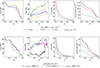 |
Fig. 6. Results from the fitted colour selections derived in Sect. 4.1, assuming the alternative magnitude and redshift selections described in Sect. 4.2. From left to right: completeness, purity, foreground failure rate, and background density as a function of zl. The assumed zl precision is δzl = 10−3. Top panels: efficiency of the griz selection, detailed in Table A.1, applied to the B20 catalogue with (S/N)E > 3 and i ≤ imax (blue solid lines), to its subsample including galaxies with i < 24.4 (red dotted lines), to the case with i < 23.4 (green dash-dotted lines), and to the sample with zg < 1.5 (orange dashed lines). Bottom panels: efficiency of the grizYEJEHE selection, detailed in Table A.2, applied to the B20 catalogue with (S/N)E > 3 and i ≤ imax (black solid lines), to its subsample with i < 23.4 (green dash-dotted lines), and to the subsample with (S/N)E > 10 (magenta dashed lines). |
In Fig. 6 we show the efficiency of the grizYEJEHE selection, computed by adopting δzl = 10−3, applied to the B20 calibration sample, with (S/N)E > 3 and i ≤ imax. We found analogous selections from the subsample with i < 23.4 and from the one with (S/N)E > 10. Specifically, in both cases, we derived higher 𝒫(zl) and lower ℱ(zl), in agreement with what we found from the griz selection. In addition, the increase in the minimum Euclid S/N does not significantly change the completeness, while the i < 23.4 limit decreases 𝒞(zl) by at most 18 percentage points. As we obtained excellent 𝒫(zl) and ℱ(zl) estimates from these tests, we conclude that both griz and grizYEJEHE selections are stable and reliable with respect to changes in the sample limiting magnitude and redshift. In addition, we note that brighter galaxy samples provide lower foreground contamination. This is expected, as faint galaxies have more scattered colour-redshift relations.
In Fig. 6 we show the density of background galaxies, nb(zl), defined as the number of selected galaxies with zg > zl per square arcmin. For both griz and grizYEJEHE selections, nb(zl) = 16 arcmin−2 at zl = 0.2 for i ≤ imax and (S/N)E > 3, decreasing with increasing zl. In both colour selections, the i < 23.4 limit implies the largest decrease in nb(zl), providing nb(zl) < 7 arcmin−2. In addition, for the griz selection, the i < 24.4 and zg < 1.5 limits provide consistent results on nb(zl), showing a difference of at most 3 arcmin−2 compared to that derived from the calibration sample. With regard to the grizYEJEHE selection, the (S/N)E > 10 limit implies a decrease in nb(zl) of up to 5 arcmin−2 at low zl, while nb(zl) becomes compatible with that derived from the calibration sample for zl > 1.
4.3. griz selection validation on real data
To further assess the reliability of the griz colour selection detailed in Sect. 4.1, we applied it to external datasets obtained from real observations. In particular, we considered the VIMOS Public Extragalactic Redshift Survey (VIPERS; Guzzo et al. 2014) Multi-Lambda Survey (VMLS) photometric catalogue by Moutard et al. (2016), including Canada-France-Hawaii Telescope Legacy Survey (CFHTLS; Hudelot et al. 2012) griz Kron aperture magnitudes (Kron 1980). This catalogue covers 22 deg2 and provides reliable photometric redshifts for more than one million galaxies with a typical accuracy of σz ≤ 0.04, and a fraction of catastrophic failures lower than 2% down to i ∼ 23. These statistics are based on VIPERS data, complemented with the most secure redshifts selected from other spectroscopic surveys. We remind that in VIPERS a colour-colour pre-selection was employed to enhance the effective sampling of the VIMOS spectrograph. Nevertheless, the VIPERS selection does not introduce any significant colour bias above z ∼ 0.6 (Guzzo et al. 2014). In addition, as we shall see in the following, the selection completeness and purity obtained from the VMLS dataset do not exhibit remarkable deviations from those obtained from other galaxy samples. In Fig. 7 we can see that, by applying the griz selection to the VMLS sample, we derived higher 𝒫(zl) and lower ℱ(zl) compared to what we found from the B20 catalogue, on average. This agrees with what we found in Sect. 4.2, as the Moutard et al. (2016) catalogue is shallower than the B20 sample. For the same reason, nb(zl) is 3 arcmin−2 lower, on average. In addition, the completeness is up to 8 percentage points higher for zl < 0.6, becoming lower for higher zl values.
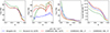 |
Fig. 7. Results of the application of the fitted colour selection based on griz photometry, reported in Table A.1, to the datasets introduced in Sect. 4.3. From left to right: completeness, purity, foreground failure rate, and background density as a function of zl. The assumed zl precision is δzl = 10−3. The griz selection is applied to the B20 catalogue with magnitude limits corresponding to those used in the calibration process (blue solid lines), to the full depth Moutard et al. (2016) catalogue (green solid lines), and to the Weaver et al. (2022) catalogue with HSC Kron, 2″ and 3″ aperture magnitudes (solid red, dashed orange and dotted black lines, respectively), for which we imposed i < 25. |
We also applied the griz selection to the COSMOS CLASSIC catalogue by Weaver et al. (2022, COSMOS20), which reaches the same photometric redshift precision as COSMOS15, namely σz/(1 + z) = 0.007, at almost one magnitude deeper. We considered griz Kron, 2″ and 3″ aperture magnitudes from HSC. In addition, we selected galaxies with a photometric redshift derived from at least 30 bands, and with i < 25, in order to consider a sample with highly reliable redshift estimates. By adopting more complex selection criteria, which may involve galaxies with photometric redshifts derived from a shared set of photometric bands, we do not expect remarkable differences in the results. Similar results for the cases with Kron, 2″ and 3″ aperture magnitudes are shown in Fig. 7. Compared to what we derived from the B20 sample, the completeness is similar, with the largest differences at zl > 0.6. In addition, ℱ(zl) is lower and 𝒫(zl) is higher for any zl. For Kron and 3″ aperture magnitudes, nb(zl) is slightly higher compared to that obtained from the B20 sample, on average. Lower nb(zl) values show up for the 2″ aperture magnitudes, which is expected as we applied the same magnitude limit for each photometric aperture definition. Indeed, for these tests we did not include aperture correction terms. Lastly, comparing the purity derived from the COSMOS20 and VMLS samples, we note that for zl > 0.3 the differences are below 1 percentage point, on average. Thus, we conclude that the griz selection provides robust and reliable results on real data.
4.4. Validation on Flagship v2.1
We tested the colour selections calibrated in Sect. 4.1 on the Euclid Flagship galaxy catalogue v2.1.10 (Euclid Collaboration, in prep.), which is currently the best simulated Euclid galaxy catalogue available. This catalogue is based on an N-body simulation with around 4 trillion particles with mass mp ∼ 109 h−1 M⊙. A flat Λ cold dark matter (ΛCDM) cosmological model was assumed, with matter density parameter Ωm = 0.319, baryon density parameter Ωb = 0.049, dark energy density parameter ΩΛ = 0.681, scalar spectral index ns = 0.96, Hubble parameter h = H0/(100 km s−1 Mpc−1) = 0.67, and standard deviation of linear density fluctuations on 8 h−1 Mpc scales σ8 = 0.83. The haloes were identified using Rockstar (Behroozi et al. 2013), and then populated with a halo occupation distribution model which was calibrated to reproduce observables such as clustering statistics as a function of galaxy luminosity. The galaxy SED templates used are the COSMOS templates from Ilbert et al. (2009), based on the models by Bruzual & Charlot (2003) and Polletta et al. (2007). In addition, galaxy photo-z probability distribution functions, namely p(zg), are included in Flagship, derived through a Nearest Neighbours Photometric Redshifts (NNPZ) pipeline (Euclid Collaboration 2020).
From the Flagship catalogue, we extracted a lightcone within RA ∈ [158 ° ,160 ° ] and Dec ∈ [12 ° ,15 ° ], considering the galaxies in the whole redshift range covered by the simulation, namely zg ∈ [0, 3]. Specifically, zg is the galaxy true redshift, and we verified that the contribution of peculiar velocities does not significantly change the results. We focused on 2″ aperture LSST ugrizy and EuclidIEYEJEHE photometry, as the simulated fluxes estimated for other ground-based surveys do not account for observational noise. Specifically, the photometric noise takes into account the depth expected in the southern hemisphere at the time of the third data release (DR3) for the Euclid Wide Survey. The LSST and Euclid 10σ magnitude limits, which are proxies for extended sources, correspond to u < 24.4, g < 25.6, r < 25.7, i < 25.0, z < 24.3, y < 23.1, IE < 25, YE < 23.5, JE < 23.5, and HE < 23.5. The fluxes we considered are not reddened due to Milky Way extinction, consistent with the analyses performed in the previous sections.
In Fig. 8, we show the application of griz and grizYEJEHE selections to Flagship. For this test, we assumed 5σ magnitude cuts for LSST ugrizy and EuclidIEYEJEHE bands. In addition, we show results from the B20 sample in Fig. 8, for which we assumed 5σ magnitude cuts rescaled from the 10σ limits listed in Euclid Collaboration (2023a, Table 1). We found that nb(zl) derived from Flagship agrees with that obtained from the B20 sample. The largest differences, of about 1 arcmin−2, arise when the grizYEJEHE selection is applied. We note that nb(zl)∼0 for zl ∼ 1.5, implying that lenses at these values of zl may not exhibit significant weak-lensing signals. Nevertheless, we verified that nb(zl) is enhanced at any zl when the selection defined for Euclid weak-lensing analyses (Laureijs et al. 2011; Euclid Collaboration 2022a) is assumed. This selection consists in a 10σ cut in the IE band, corresponding to IE < 25 for a 2″ aperture, yielding a galaxy density of around 39 arcmin−2 when applied to the Flagship dataset. In fact, in this case nb(zl) ranges from 30 arcmin−2 at low zl to 3 arcmin−2 at zl = 1.5.
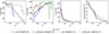 |
Fig. 8. Application of the calibrated colour selections to the Flagship simulated sample described in Sect. 4.4. From left to right: completeness, purity, foreground failure rate, and background density as a function of zl, from the fitted colour selections based on griz and grizYEJEHE bands, adopting 5σ magnitude limits. The assumed zl precision is δzl = 10−3. The solid blue and solid black lines represent the griz and grizYEJEHE selections, respectively, applied to the B20 catalogue. The dashed red and dashed green curves represent the griz and grizYEJEHE selections, respectively, applied to the Flagship v2.1 catalogue (Euclid Collaboration, in prep.). |
As shown in Fig. 8, on average we obtained higher 𝒫(zl) and lower ℱ(zl) for zl < 1 from Flagship, compared to what we derived from the B20 sample. For the griz selection case, 𝒞(zl) agrees with that derived from the B20 sample, with the largest differences, of up to 16 percentage points, at zl ∼ 0.5. Larger differences in 𝒞(zl) are obtained from the grizYEJEHE selection. From Flagship we obtained 𝒞(zl) up to 10 percentage points larger for zl < 0.6, and up to 50 percentage points larger for higher zl. We verified that this discrepancy in the completeness, in the case of the grizYEJEHE selection, is not significantly attenuated through the assumption of 3σ and 10σ magnitude limits on both B20 and Flagship catalogues. Analogous results were obtained by assuming limits corresponding to the magnitude distribution peaks derived from the B20 catalogue, namely g < 24.9, r < 24.6, i < 24.3, z < 24.1, YE < 23.8, JE < 23.6, and HE < 23.5. Moreover, we verified that the grizYEJEHE selection completeness does not remarkably vary by assuming the Euclid weak-lensing selection defined above, namely IE < 25. Similar results are obtained by considering the photometric errors expected for the DR2 of the Euclid Wide Survey, assuming the corresponding 3σ, 5σ, and 10σ magnitude cuts. For each of the alternative magnitude cuts discussed in this section, we found that the grizYEJEHE selection yields a purity up to 3 percentage points higher at zl > 1.2 when it is applied to the B20 catalogue, compared to what is derived from Flagship. At zl < 1.2, instead, the purity obtained from B20 is 1 percentage point lower, on average. Furthermore, the alternative magnitude cuts do not remarkably impact the selection purity at any zl.
We additionally adopted SDSS fluxes, which do not include photometric noise, in place of LSST fluxes in Flagship. In this case, the completeness is up to 35 percentage points larger than that derived from the B20 sample, and the purity approaches 100% for zl > 1, which is similar to what we derived from the B20 sample (see Fig. 8). Thus, the selection based on SDSS photometry is less complete and purer compared to that obtained from LSST magnitudes.
Differences in the completeness derived from the Flagship and B20 samples may originate from distinct assumptions on the physical properties of the galaxies, such as dust extinction, stellar age, nebular emission lines, or on the assumed intrinsic spectral energy distributions. This could be indicated by a different fraction of star forming galaxies in the two samples. Following B20, galaxies are classified as star forming if the following condition is satisfied,
 (8)
(8)
where sSFR is the specific star formation rate, derived from the best SED template in the catalogue by B20. We verified that, for zg > 1, the fraction of star forming galaxies in Flagship is consistent within 1 percentage point with that derived from the catalogue by B20. Thus, we conclude that the completeness differences between the Flagship and B20 samples are not due to different star forming galaxy populations. We also verified that the log10(sSFR/yr−1) distributions derived from the two datasets are compatible, having peaks at ∼ − 8.13 and ∼ − 8.35 in B20 and Flagship, respectively. The agreement of these peak values is well within 1σ of the log10(sSFR/yr−1) distributions. We will be able to further investigate such completeness differences through the analysis of the first data release of the Euclid Deep Survey.
4.5. Comparison with photo-z selections
To compare the colour selections derived in this work to selections based on the galaxy p(zg), commonly referred to as photo-z selections, we analysed the Flagship sample described in Sect. 4.4. We considered only the galaxies with a p(zg) estimate obtained with the NNPZ pipeline (Euclid Collaboration 2020). The NNPZ photo-zs are designed to work well for galaxies that are expected to be used in core Euclid weak-lensing science, namely with 5σ limits on the IE band. Thus we imposed IE < 25.75, along with 5σ limits on the YEJEHE bands, namely YE < 24.25, JE < 24.25, HE < 24.25. Specifically, we adopted the following photo-z selection,
 (9)
(9)
where  is the minimum of the interval containing 95% of the probability around the first mode of p(zg), namely
  . We chose
  in order to derive 𝒫(zl) values which are compatible with those obtained from colour selections. We verified that adding a condition on the width of p(zg) in Eq. (9) does not impact the results. Specifically, for the latter test, we considered the additional condition 𝒜 > 𝒜min, where 𝒜 is the integrated probability around
  , computed within the redshift points, which are the closest to
  , having an associated probability of
  . We verified that imposing 𝒜min = 0 or 𝒜min = 0.8 leads to compatible purity values with sub-percent differences on average. However, 𝒜min = 0.8 lowers the photo-z selection completeness by around 20 percentage points at all zl. Consequently, we assumed 𝒜min = 0.
To perform a fair comparison of colour and photo-z selections, we considered only the grizYEJEHE colour selection in this section. This is because photo-zs in Flagship were derived from the combination of ground-based and Euclid photometry. In Fig. 9, we show that the grizYEJEHE selection provides, on average, a completeness 15 percentage points lower than that of the photo-z selection, with similar contamination. By combining grizYEJEHE and photo-z selections, through the logical operator ∨, the completeness increases by up to 10 percentage points with respect to the case of photo-z selection alone, amounting to 𝒞(zl)∼95% for zl < 1.4. These preliminary tests confirm the importance of the combination of colour and photo-z selections, as it leads to significantly more complete background galaxy samples. We also remark that increasing the selection completeness is key to reduce biases in the shear calibration parameters due to background selections, as we shall detail in Sect. 4.6. The analysis of Euclid data will allow for a detailed investigation of the optimal photo-z selections for galaxy cluster weak-lensing analyses, outlining the synergies with colour selections. For example, colour selections applied to Euclid data could provide more robust background samples for massive or nearby galaxy clusters, as derived by Medezinski et al. (2018). Leveraging colour selections also serves as a valuable cross-validation method for addressing the effect of unknown systematic uncertainties in photo-z estimates. Lastly, Fig. 9 shows the selection based only on the first mode of p(zg). Specifically, in this case we selected the galaxies with  . Despite 𝒞(zl) > 90% at all zl, the purity is up to 10 percentage points lower than that obtained from the grizYEJEHE selection.
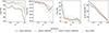 |
Fig. 9. Comparison of colour and photo-z selections. From left to right: completeness, purity, foreground failure rate, and background density as a function of zl, obtained from Flagship v2.1. The solid black lines represent the grizYEJEHE selection. The dashed green lines show the combination, through the ∨ logical operator, of grizYEJEHE and photo-z selection (Eq. (9)). The dashed red lines represent the photo-z selection, while the dotted black lines represent the selection based on the p(zg) mode. |
4.6. Impact on shear measurements
In cluster weak-lensing analyses, the inclusion of foreground sources in the shear measurements may significantly dilute the signal (Broadhurst et al. 2005; Medezinski et al. 2007; Sifón et al. 2015; McClintock et al. 2019). As discussed in the previous sections, the calibrated colour selections provide 𝒫(zl) < 1. To assess the impact of impurities on shear measurements, we can express the cluster reduced tangential shear unaffected by contamination as follows (Dietrich et al. 2019):
 (10)
(10)
where gt(zl) is the measured cluster reduced tangential shear at redshift zl. As the calibrated colour selections yield 𝒫(zl) > 0.97, we expect at most a 3% bias on the reduced tangential shear. In addition, as discussed in Sect. 4.3, 𝒫(zl) derived from different observed datasets with only ground-based photometry shows a scatter below 1 percentage point. This scatter in 𝒫(zl) is lower than the systematic uncertainty on galaxy shape measurements for stage III surveys, as we shall discuss in the following. We remark that 𝒫(zl) is derived from reference fields, while galaxy clusters are overdense compared to the cosmic mean. Thus, contamination from cluster galaxies must be properly accounted for in Eq. (10) (see, e.g. Gruen et al. 2014; Dietrich et al. 2019). Nevertheless, such contamination is consistent with zero in the typical cluster-centric radial range adopted for mass calibration, namely at radii larger than 300 h−1 kpc (see, e.g. Medezinski et al. 2018; Bellagamba et al. 2019).
Furthermore, galaxy shear calibration is usually statistically derived, based on observed and simulated galaxy samples. Nevertheless, through galaxy cluster background selections, some galaxy populations may be systematically excluded. This may invalidate the statistical estimate of the shape multiplicative bias, namely m, depending on the shear measurement technique and on the actual properties of the data (Heymans et al. 2012; Miller et al. 2013; Hildebrandt et al. 2016).
The typical uncertainty on m found for stage III surveys ranges in the interval δm ∈ [1 × 10⁻², 3 × 10⁻²] (see, e.g. Jarvis et al. 2016; Melchior et al. 2017; Giblin et al. 2021). To assess the impact of colour selections on m, we considered the shape catalogues of Heymans et al. (2012), based on CFHTLS, and of Mandelbaum et al. (2018), based on the HSC Subaru Strategic Program (HSC-SSP; Miyazaki et al. 2018; Aihara et al. 2018). Throughout this section, we adopted a lens redshift of zl = 0.5. By applying the griz selection calibrated in this work, we derived a shift in the mean shear multiplicative bias of Δm = 7 × 10⁻³ in CFHTLS and of Δm = −2 × 10⁻³ in HSC-SSP. In addition, the Oguri et al. (2012) and Medezinski et al. (2018) colour selections provide Δm = −3 × 10⁻³ and Δm = −1 × 10⁻² from CFHTLS, respectively, while from HSC-SSP we obtained Δm = −5 × 10⁻³ and Δm = −7 × 10⁻³, respectively. Thus, galaxy population differences due to colour cuts provide systematic effects that are within the typical m uncertainty in stage III surveys. By combining colour and photo-z selections, we expect Δm to become closer to zero. In Euclid-like surveys, shear has to be calibrated within an accuracy of 2 × 10⁻³ (Cropper et al. 2013). As we discussed in Sect. 4.5, the combination of grizYEJEHE and photo-z selections leads to 90% background completeness in the Euclid Wide Survey, on average; thus, we may expect the bias on m to be subdominant with respect to the required shear accuracy. Indeed, let us assume that 90% of galaxies, selected through the combination of grizYEJEHE and photo-z selections, have an average m similar to that derived from stage III surveys, namely ⟨m⟩ = 0.01. We assume that the remaining 10% of galaxies have a very biased m, namely ⟨m⟩ = 0.02, compared to the selected population. This would imply a systematic error of Δm = 10−3 in the average m of the selected population. We will delve deeper into these variations in m by examining the first data releases of the Euclid surveys.
4.7. Selection efficiency with missing bands
In this work, we derived colour selections based on griz and grizYEJEHE photometry. In some cases, however, the full ground-based griz photometry may be not available. For example, the DES Year 3 galaxy shape catalogue was not based on g band (Gatti et al. 2021), due to issues in the point spread function estimation (Jarvis et al. 2021). Thus, we investigated the efficiency of griz and grizYEJEHE selections in the case of a missing band, based on the B20 calibration sample described in Sect. 2. In performing this test, we excluded the colour conditions in Tables A.1 and A.2 containing the chosen missing bands. In Fig. 10 we show that, in the case of ground-only observations, the absence of the r band implies the largest completeness decrease, providing 𝒞(zl) < 60%. In addition, the zl range is substantially reduced, corresponding to zl ∈ [0.2, 0.6]. Also the absence of i and z bands implies a reduction of the maximum zl for the ground-based selection, corresponding to zl = 0.7 and zl = 0.6, respectively, and a completeness decrease of up to 10 and 20 percentage points, respectively. On average, a 20 percentage points drop in completeness is found in absence of g band photometry. Nevertheless, in the latter case the zl range is not reduced. We remark that the considered samples differ from case to case, as they contain only galaxies with photometry available in the required bands.
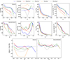 |
Fig. 10. Colour selection results, obtained from the B20 catalogue, in case of missing z (solid red), i (solid green), r (dashed orange), and g (dashed grey) bands. The blue curves represent the results from the griz and grizYEJEHE selections reported in Tables A.1 and A.2. Top panels, from left to right: completeness, purity, foreground failure rate, and background density are shown, in the case of ground-only photometry. Middle panels: colour selections from the combination of ground-based and Euclid photometry. The plot structure is analogous to that of top panels. Bottom panels: difference between |

In Fig. 10 we show the effect of missing photometric bands on the combination of ground-based and Euclid observations. In this case, the lack of r band does not imply changes in 𝒞(zl) for zl > 1. In the absence of i band, 𝒞(zl) significantly decreases for zl ≳ 0.7, being below 30%, while the zl range is not reduced. A zl range reduction is obtained in the case of missing z or g bands, as we derived zl ∈ [0.2, 1.1] and zl ∈ [0.2, 1.3], respectively. On average, in the case of the combination of ground-based and Euclid observations, the largest completeness decrease is caused by the lack of the g band.
In this section, we defined colour selections with missing g, r, i, or z band, as subsets of the colour conditions defining the griz and grizYEJEHE selections. In order to assess the difference between the selections defined by such subsets and those that would be derived from the colour selection calibration described in Sect. 3, we compute  for each case. In Fig. 10, we show the difference between
  and 𝒞, the latter being derived by subsets of the colour conditions defining griz and grizYEJEHE selections. In the ground-only case, the lack of r band provides the largest 𝒞 underestimation, as
  15 percentage points for zl ∈ [0.3, 0.5]. Nevertheless, in case of other missing bands, the average
  is close to 0. The same holds for the combination of ground-based and Euclid photometry. We conclude that griz and grizYEJEHE selections provide robust results in the case of a missing band, except for ground-only observations without the r band, for which a dedicated calibration might be needed.
5. Comparison with literature ground-based selections
Based on the B20 sample considered in Sect. 4.1, we compared our griz colour selection to those derived by Medezinski et al. (2010, 2018) and Oguri et al. (2012), which are also implemented in COMB-CL. As detailed below, for each of these selections, we considered two versions. One includes all the colour conditions provided by the corresponding authors, while the other comprises only a subsample of such conditions, providing lower foreground contamination. COMB-CL includes both versions of each colour selection.
Medezinski et al. (2010) derived colour selections for three massive clusters, identified through deep Subaru imaging, by maximising their weak-lensing signal. COMB-CL provides the selection calibrated for the A1703 cluster at redshift zl ∼ 0.26, as this is the one based on gri photometry. This selection is expressed as follows,
![Mathematical equation: $$ \begin{aligned} \big [\,&(g-r) < 2.17\,(r-i) - 0.37\,\, , \nonumber \\&(g-r) < -0.6\,(r-i) + 1.85\,\,, \,\, (r-i) > 0.3 \,\big ] \,\, \vee \end{aligned} $$](/articles/aa/full_html/2024/04/aa48743-23/aa48743-23-eq50.gif) (11)
(11)
![Mathematical equation: $$ \begin{aligned} \big [\,&(g-r) < -0.4\,(r-i) + 0.47 \,\,, \,\, (r-i) < 0.3 \,\big ]\,\,\vee \,\,\nonumber \\&(r-i) < -0.06, \end{aligned} $$](/articles/aa/full_html/2024/04/aa48743-23/aa48743-23-eq51.gif) (12)
(12)
where ∧ is the logical “and” operator. Notably, Eq. (11) defines the red background sample, namely the galaxies redder than cluster galaxies, while Eq. (12) defines the blue background sample. In Fig. 11, we can see that this selection provides 𝒞(zl) = 60%, which is 20 percentage points lower than that provided by the griz selection calibrated in this work. In addition, from the Medezinski et al. (2010) selection we derived 𝒫(zl) > 96%, which is slightly lower than that obtained from the griz selection discussed in Sect. 4.1. Foreground contamination can be attenuated by considering the red sample selection only, namely Eq. (11), as shown in Fig. 11. In this case, however, the completeness is lowered by 20 percentage points. In Fig. 12 (upper panel), we show a comparison between the selection by Medezinski et al. (2010), namely Eqs. (11) and (12), and our griz selection in the (r − i)−(g − r) colour-colour space, by assuming zl = 0.26. Within this colour-colour space, we obtained 𝒞(zl) = 55% and 𝒫(zl) = 98% from the griz selection, while through the Medezinski et al. (2010) selection we found 𝒞(zl) = 62% and 𝒫(zl) = 95%. We remark that the full set of colour conditions defining the griz selection yields 80% completeness for zl = 0.26, and that a calibration based on gri bands only would yield larger completeness values in the (r − i)−(g − r) space (see Sect. 4.7). In addition, Fig. 12 shows that the griz selection extends the selected region defined by Eq. (11), thus enhancing the red background sample compared to Medezinski et al. (2010). On the other hand, the griz selection shows a more conservative definition of the blue background sample, compared to Eq. (12).
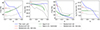 |
Fig. 11. Comparison of the griz selection described in Sect. 4.1 with literature colour selections. From left to right: completeness, purity, foreground failure rate, and background density, derived from the B20 catalogue. The blue solid lines represent the griz selection derived in this work. The red curves refer to the Medezinski et al. (2010) selection, where the solid lines are given by Eqs. (11)–(12), while the dashed lines are given by Eq. (11). The green curves represent the results from the Oguri et al. (2012) selection, where the solid lines are given by Eqs. (13)–(16), while the dashed lines are given by Eqs. (13)–(15). The grey curves refer to the Medezinski et al. (2018) selection, where the solid lines are given by Eqs. (17)–(18), while the dashed lines are given by Eq. (17). |
Oguri et al. (2012) calibrated a selection based on gri photometry from the COSMOS catalogue by Ilbert et al. (2009), providing reliable results for lenses at redshift zl ≲ 0.7. This selection is expressed as
 (13)
(13)
 (14)
(14)
 (15)
(15)
 (16)
(16)
The inclusion of Eq. (16) does not provide significant improvement in the completeness, causing a lower selection purity (Covone et al. 2014). In fact, Fig. 11 shows that the selection including Eqs. (13)–(16) provides sub-percent improvements in 𝒞(zl), compared to the selection including Eqs. (13)–(15) only, while 𝒫(zl) and ℱ(zl) are up to 1 percentage point lower and higher, respectively. With respect to the griz selection calibrated in this work, the Oguri et al. (2012) selection provides a purity which is up to 5 percentage points lower. This explains the higher completeness values for zl > 0.6. For lower zl, the Oguri et al. (2012) selection provides a completeness up to 35 percentage points lower, which is expected as the selection by Oguri et al. (2012) was calibrated for clusters at zl ∼ 0.7. Similarly to the comparison with the Medezinski et al. (2010) selection discussed above, in Fig. 12 (lower panel) we compare the griz and Oguri et al. (2012) selections in the (r − i)−(g − r) colour-colour space, assuming zl = 0.6. We obtained 𝒞(zl) = 27% and 𝒫(zl) = 98% from the griz selection, while with the Oguri et al. (2012) selection we found 𝒞(zl) = 60% and 𝒫(zl) = 94%. With respect to what we found by comparing griz and Medezinski et al. (2010) selections at zl = 0.26, the decrease in completeness due to a purity enhancement is much larger at zl = 0.6. This depends on the overlap of the foreground and background galaxy distributions in the (r − i)−(g − r) space. In addition, we remark that the calibration process presented in Sect. 3 excludes redundant colour conditions. This may partially explain the 27% completeness found in the case of the griz selection.
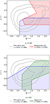 |
Fig. 12. Comparison of colour selections in the (r − i)−(g − r) colour-colour space. The solid grey contours indicate the 68%, 95%, and 99% galaxy number density in the calibration sample, described in Sect. 2. The blue shaded areas represent the regions excluded by applying the griz selection calibrated in Sect. 4.1. Completeness and purity of the selections are reported in the legends. For the griz selection, 𝒞 and 𝒫 are computed by considering the colour conditions in Table A.1 which are defined in the (r − i)−(g − r) space. Top panel: the red hatched area shows the region excluded through the Medezinski et al. (2010) selection, and zl = 0.26 is assumed. Bottom panel: the green hatched area shows the region excluded through the Oguri et al. (2012) selection, and zl = 0.6 is assumed. |
Medezinski et al. (2018) calibrated a colour selection based on HSC observations, including griz bands, following an approach similar to Medezinski et al. (2010). This colour selection is expressed as
![Mathematical equation: $$ \begin{aligned} \Bigg [\,&(g-i) < 2.276 \, (r-z) - 0.152 + a(z_{\rm l}) \,\,, \nonumber \\&(g-i) < \frac{1}{2.276} \, (r-z) + b(z_{\rm l}) \left(1+\frac{1}{2.276^2}\right) - \frac{0.152}{2.276^2} \,\,, \nonumber \\&(r-z) > 0.5 \,\,, \nonumber \\&z > 21\,\Bigg ]\,\,\vee \end{aligned} $$](/articles/aa/full_html/2024/04/aa48743-23/aa48743-23-eq56.gif) (17)
(17)
![Mathematical equation: $$ \begin{aligned} \Bigg \{\,&(r-z) < -0.0248\,z + 1.604+c(z_{\rm l}) \,\,\vee \nonumber \\&\Bigg [\,(g-i)<\frac{1}{2.276}\,(r-z)+d(z_{\rm l}) \left(1+\frac{1}{2.276^2}\right) - \frac{0.152}{2.276^2} \,\,, \nonumber \\&(g-i)<4\,\Bigg ]\,\,\vee \nonumber \\&(r-z) < 0.5\,\,\vee \nonumber \\&z> 22\,\Bigg \}, \end{aligned} $$](/articles/aa/full_html/2024/04/aa48743-23/aa48743-23-eq57.gif) (18)
(18)
where
 (19)
(19)
 (20)
(20)
 (21)
(21)
 (22)
(22)
Similarly to Medezinski et al. (2010), Eqs. (17) and (18) define the red and blue background samples, respectively. This selection provides a much larger amount of contamination compared to that derived in this work, reaching 𝒫(zl) < 90% for zl > 0.7, as shown in Fig. 11. However, by considering the red sample selection only, the purity improves by up to 6 percentage points. In the latter case, compared to the griz selection detailed in Table A.1, 𝒞(zl) is up to 50 percentage points lower for zl < 0.7. For higher zl, the lower purity from the Medezinski et al. (2018) selection allows for higher completeness values.
In Fig. 13 we show the redshift distributions of the galaxies selected through the griz, Medezinski et al. (2010, 2018) and Oguri et al. (2012) selections, assuming different zl values. At zl = 0.26, the griz selection shows a larger number of galaxies, of the order of 103, which are correctly identified as background objects with zg < 0.6, compared to Medezinski et al. (2010). This results in the larger completeness of the griz selection shown in Fig. 11. At zl = 0.6, where the griz and Oguri et al. (2012) selections have the same completeness (see Fig. 11), the griz selection is less complete at zg > 1.5 and more complete at lower redshifts, compared to Oguri et al. (2012). At zl = 0.8, where the griz selection is remarkably purer than that by Medezinski et al. (2018), a notable incompleteness of the griz selection is evident at any zg, compared to Medezinski et al. (2018). In fact, for the case of the griz selection, Fig. 13 shows that the number of rejected galaxies at high redshift increases with the number of excluded foreground galaxies. This reflects the overlapping of foreground and background galaxy distributions in the considered colour-colour spaces.
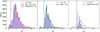 |
Fig. 13. From left to right: number of selected galaxies as a function of zg assuming zl = 0.26, zl = 0.6, and zl = 0.8. The zl values are represented by vertical black dashed lines. The blue histograms represent the griz selection calibrated in this work. The galaxy redshift distributions derived with the Medezinski et al. (2010, 2018) and Oguri et al. (2012), selections are represented by red, green, and grey hatched histograms, respectively. |
6. Discussion and conclusions
We developed a method to derive optimal galaxy colour selections for cluster weak-lensing analyses, given any set of photometric bands. To this aim, we considered all the available colour-colour combinations. Based on the galaxy catalogue by B20, we calibrated selections based on ground-based griz and EuclidYEJEHE bands, with purity higher than 97%. Specifically, we showed that the griz selection provides a completeness between 30% and 84%, in the lens limiting redshift range zl ∈ [0.2, 0.8]. The inclusion of EuclidYEJEHE bands, leading to a grizYEJEHE selection, improves the completeness by up to 25 percentage points in this zl range, allowing for a galaxy selection up to zl = 1.5. In addition, for the first time in the literature, we expressed such selections as a continuous function of zl. In the following, we summarise the main results obtained from the tests presented in Sects. 4 and 5.
-
The calibrated colour selections, described in Sect. 4.1, are stable with respect to changes in the sample limiting magnitudes and redshift.
-
By applying the griz selection to the VMLS catalogue by Moutard et al. (2016) and to the COSMOS20 catalogue by Weaver et al. (2022), we derived completeness and purity estimates that are consistent with those obtained from the calibration sample by B20. Consequently, the calibrated selections provide stable results by assuming alternative photometric aperture definitions, obtained from different ground-based telescopes.
-
The application of griz and grizYEJEHE selections to the simulated Euclid Flagship galaxy catalogue v2.1.10 (Euclid Collaboration, in prep.) provided a purity of around 99%, on average, which is higher than that obtained from the B20 catalogue. The completeness from the Flagship and B20 samples is compatible in the griz selection case, while the grizYEJEHE selection provides up to 50 percentage points higher completeness from Flagship. We verified that this discrepancy does not depend on magnitude limits. In addition, we found no significant differences in the star forming galaxy fraction from the Flagship and B20 samples. A calibration of the grizYEJEHE selection based on the Euclid Deep Survey will allow for a more thorough investigation of these completeness differences.
-
Based on the Flagship sample, we combined the calibrated colour selections with photo-z selections based on the p(zg) shape. We showed that in this case the completeness is up to 95%.
-
We found no significant systematic effects on the multiplicative shear bias due to colour selections for stage III surveys. The first Euclid data releases will provide further insights into the influence of background selections on this bias.
-
The calibrated colour selections provide robust results in the case of a missing band from ground-based observations, except for those without the r band, for which a dedicated calibration might be needed.
-
Compared to the ground-based colour selections provided by Medezinski et al. (2010, 2018) and Oguri et al. (2012), the griz selection derived in this work is purer at high redshift and more complete at low redshift.
One potential enhancement to the calibration presented in this work could entail the inclusion of a magnitude dependence in the colour cuts. This might mitigate the impact of large photometric scatter at faint magnitudes (see, e.g. Schrabback et al. 2021). In addition, enhancing the set of photometric bands in the calibration sample, for example by including the LSST y band, could remarkably improve the effectiveness of the colour selections. The performance of colour selections could further improve through dedicated calibration samples. Ongoing spectroscopic programmes are specifically designed to calibrate the relationship between galaxy colours and redshifts to match the depth of the Euclid survey (Euclid Collaboration 2022c).
Furthermore, the colour selections presented in this work could improve the shear calibration in cluster weak-lensing analyses. The lensing signal from galaxy clusters differs from that of large scale structure in ways that affect both shear and photometric measurements. The dense cluster environment causes increased blending among light sources, due to both galaxy blends (Simet & Mandelbaum 2015; Everett et al. 2022) and the presence of diffuse intra-cluster light (Gruen et al. 2019; Kluge et al. 2020; Sampaio-Santos et al. 2021). In addition, cluster lines of sight exhibit characteristically stronger shear, especially at small scales (McClintock et al. 2019; Ingoglia et al. 2022). These effects can lead to distinct biases in shear measurements compared to those obtained from calibrations primarily designed for cosmic shear analyses. Through the combination of colour and photo-z selections, cluster shear calibration and mass bias can be assessed based on dedicated, multi-band cluster image simulations (see, e.g. Hernández-Martín et al. 2020).
IE band observations are supplied by the Euclid Visible Imager (VIS; Cropper et al. 2016), while YEJEHE photometry is provided by the Near-Infrared Spectrometer and Photometer (NISP; Euclid Collaboration 2022b).
UNIONS is carried out with the Subaru Telescope (Iye et al. 2004), the Canada-France-Hawaii Telescope (CFHT; Gwyn 2012), and the Panoramic Survey Telescope and Rapid Response System (Pan-STARRS; Chambers et al. 2016). More information at https://www.skysurvey.cc/news/
Acknowledgments
The Euclid Consortium acknowledges the European Space Agency and a number of agencies and institutes that have supported the development of Euclid, in particular the Academy of Finland, the Agenzia Spaziale Italiana, the Belgian Science Policy, the Canadian Euclid Consortium, the French Centre National d’Etudes Spatiales, the Deutsches Zentrum für Luft- und Raumfahrt, the Danish Space Research Institute, the Fundação para a Ciência e a Tecnologia, the Ministerio de Ciencia e Innovación, the National Aeronautics and Space Administration, the National Astronomical Observatory of Japan, the Netherlandse Onderzoekschool Voor Astronomie, the Norwegian Space Agency, the Romanian Space Agency, the State Secretariat for Education, Research and Innovation (SERI) at the Swiss Space Office (SSO), and the United Kingdom Space Agency. A complete and detailed list is available on the Euclid website (https://www.euclid-ec.org) We thank W. Hartley for his valuable advice, which remarkably enhanced the quality of this work. G.C. and L.M. acknowledge the support from the grant ASI n.2018-23-HH.0. L.M. and F.M. acknowledge the financial contribution from the grant PRIN-MUR 2022 20227RNLY3 “The concordance cosmological model: stress-tests with galaxy clusters” supported by Next Generation EU. L.B. acknowledges financial support from PRIN-MIUR 2017–20173ML3WW_001. M.S. acknowledges financial contributions from contract ASI-INAF n.2017-14-H.0, contract INAF mainstream project 1.05.01.86.10, and INAF Theory Grant 2023: Gravitational lensing detection of matter distribution at galaxy cluster boundaries and beyond (1.05.23.06.17). G.C. thanks the support from INAF Theory Grant 2022: Illuminating Dark Matter using Weak Lensing by Cluster Satellites, PI: Carlo Giocoli. This work has made use of CosmoHub (Carretero et al. 2017; Tallada et al. 2020). CosmoHub has been developed by the Port d’Informació Científica (PIC), maintained through a collaboration of the Institut de Física d’Altes Energies (IFAE) and the Centro de Investigaciones Energéticas, Medioambientales y Tecnológicas (CIEMAT) and the Institute of Space Sciences (CSIC & IEEC), and was partially funded by the “Plan Estatal de Investigación Científica y Técnica y de Innovación” program of the Spanish government.
References
- Abbott, T. M. C., Aguena, M., Alarcon, A., et al. 2020, Phys. Rev. D, 102, 023509 [Google Scholar]
- Aihara, H., Armstrong, R., Bickerton, S., et al. 2018, PASJ, 70, S8 [NASA ADS] [Google Scholar]
- Applegate, D. E., von der Linden, A., Kelly, P. L., et al. 2014, MNRAS, 439, 48 [Google Scholar]
- Baltz, E. A., Marshall, P., & Oguri, M. 2009, JCAP, 2009, 015 [Google Scholar]
- Behroozi, P. S., Wechsler, R. H., & Wu, H.-Y. 2013, ApJ, 762, 109 [NASA ADS] [CrossRef] [Google Scholar]
- Bellagamba, F., Sereno, M., Roncarelli, M., et al. 2019, MNRAS, 484, 1598 [Google Scholar]
- Bisigello, L., Kuchner, U., Conselice, C. J., et al. 2020, MNRAS, 494, 2337 [NASA ADS] [CrossRef] [Google Scholar]
- Broadhurst, T., Takada, M., Umetsu, K., et al. 2005, ApJ, 619, L143 [NASA ADS] [CrossRef] [Google Scholar]
- Bruzual, G., & Charlot, S. 2003, MNRAS, 344, 1000 [NASA ADS] [CrossRef] [Google Scholar]
- Carretero, J., Tallada, P., Casals, J., et al. 2017, Proceedings of the European Physical Society Conference on High Energy Physics, 5-12 July, 488 [CrossRef] [Google Scholar]
- Chambers, K. C., Magnier, E. A., Metcalfe, N., et al. 2016, arXiv e-prints [arXiv:1612.05560] [Google Scholar]
- CHEX-MATE Collaboration (Arnaud, M., et al.) 2021, A&A, 650, A104 [NASA ADS] [CrossRef] [EDP Sciences] [Google Scholar]
- Costanzi, M., Rozo, E., Simet, M., et al. 2019, MNRAS, 488, 4779 [NASA ADS] [CrossRef] [Google Scholar]
- Covone, G., Sereno, M., Kilbinger, M., & Cardone, V. F. 2014, ApJ, 784, L25 [NASA ADS] [CrossRef] [Google Scholar]
- Cropper, M., Hoekstra, H., Kitching, T., et al. 2013, MNRAS, 431, 3103 [Google Scholar]
- Cropper, M., Pottinger, S., Niemi, S., et al. 2016, in Space Telescopes and Instrumentation 2016: Optical, Infrared, and Millimeter Wave, eds. H. A. MacEwen, G. G. Fazio, M. Lystrup, et al., SPIE Conf. Ser., 9904, 99040Q [NASA ADS] [Google Scholar]
- Diemer, B., & Kravtsov, A. V. 2014, ApJ, 789, 1 [NASA ADS] [CrossRef] [Google Scholar]
- Dietrich, J. P., Bocquet, S., Schrabback, T., et al. 2019, MNRAS, 483, 2871 [Google Scholar]
- Eckert, D., Ettori, S., Robertson, A., et al. 2022, A&A, 666, A41 [NASA ADS] [CrossRef] [EDP Sciences] [Google Scholar]
- Euclid Collaboration (Adam, R., et al.) 2019, A&A, 627, A23 [NASA ADS] [CrossRef] [EDP Sciences] [Google Scholar]
- Euclid Collaboration (Desprez, G., et al.) 2020, A&A, 644, A31 [EDP Sciences] [Google Scholar]
- Euclid Collaboration (Pocino, A., et al.) 2021, A&A, 655, A44 [NASA ADS] [CrossRef] [EDP Sciences] [Google Scholar]
- Euclid Collaboration (Scaramella, R., et al.) 2022a, A&A, 662, A112 [NASA ADS] [CrossRef] [EDP Sciences] [Google Scholar]
- Euclid Collaboration (Schirmer, M., et al.) 2022b, A&A, 662, A92 [NASA ADS] [CrossRef] [EDP Sciences] [Google Scholar]
- Euclid Collaboration (Saglia, R., et al.) 2022c, A&A, 664, A196 [NASA ADS] [CrossRef] [EDP Sciences] [Google Scholar]
- Euclid Collaboration (Bisigello, L., et al.) 2023a, MNRAS, 520, 3529 [NASA ADS] [CrossRef] [Google Scholar]
- Euclid Collaboration (Sereno, M., et al.) 2023b, A&A, submitted [Google Scholar]
- Everett, S., Yanny, B., Kuropatkin, N., et al. 2022, ApJS, 258, 15 [NASA ADS] [CrossRef] [Google Scholar]
- Gatti, M., Sheldon, E., Amon, A., et al. 2021, MNRAS, 504, 4312 [NASA ADS] [CrossRef] [Google Scholar]
- Giblin, B., Heymans, C., Asgari, M., et al. 2021, A&A, 645, A105 [NASA ADS] [CrossRef] [EDP Sciences] [Google Scholar]
- Gruen, D., Seitz, S., Brimioulle, F., et al. 2014, MNRAS, 442, 1507 [CrossRef] [Google Scholar]
- Gruen, D., Zhang, Y., Palmese, A., et al. 2019, MNRAS, 488, 4389 [NASA ADS] [CrossRef] [Google Scholar]
- Gunn, J. E., Carr, M., Rockosi, C., et al. 1998, AJ, 116, 3040 [NASA ADS] [CrossRef] [Google Scholar]
- Guzzo, L., Scodeggio, M., Garilli, B., et al. 2014, A&A, 566, A108 [NASA ADS] [CrossRef] [EDP Sciences] [Google Scholar]
- Gwyn, S. D. J. 2012, AJ, 143, 38 [Google Scholar]
- Hernández-Martín, B., Schrabback, T., Hoekstra, H., et al. 2020, A&A, 640, A117 [EDP Sciences] [Google Scholar]
- Heymans, C., & Heavens, A. 2003, MNRAS, 339, 711 [CrossRef] [Google Scholar]
- Heymans, C., Van Waerbeke, L., Miller, L., et al. 2012, MNRAS, 427, 146 [Google Scholar]
- Hildebrandt, H., Choi, A., Heymans, C., et al. 2016, MNRAS, 463, 635 [Google Scholar]
- Hoekstra, H., Mahdavi, A., Babul, A., & Bildfell, C. 2012, MNRAS, 427, 1298 [NASA ADS] [CrossRef] [Google Scholar]
- Hudelot, P., Cuillandre, J. C., Withington, K., et al. 2012, VizieR Online Data Catalog: II/317 [Google Scholar]
- Ibata, R. A., McConnachie, A., Cuillandre, J.-C., et al. 2017, ApJ, 848, 128 [Google Scholar]
- Ilbert, O., Capak, P., Salvato, M., et al. 2009, ApJ, 690, 1236 [NASA ADS] [CrossRef] [Google Scholar]
- Ingoglia, L., Covone, G., Sereno, M., et al. 2022, MNRAS, 511, 1484 [NASA ADS] [CrossRef] [Google Scholar]
- Ivezic, Z., Axelrod, T., Brandt, W. N., et al. 2008, Serb. Astron. J., 176, 1 [Google Scholar]
- Iye, M., Karoji, H., Ando, H., et al. 2004, PASJ, 56, 381 [NASA ADS] [Google Scholar]
- Jarvis, M., Sheldon, E., Zuntz, J., et al. 2016, MNRAS, 460, 2245 [Google Scholar]
- Jarvis, M., Bernstein, G. M., Amon, A., et al. 2021, MNRAS, 501, 1282 [Google Scholar]
- Klein, M., Israel, H., Nagarajan, A., et al. 2019, MNRAS, 488, 1704 [NASA ADS] [CrossRef] [Google Scholar]
- Kluge, M., Neureiter, B., Riffeser, A., et al. 2020, ApJS, 247, 43 [Google Scholar]
- Kron, R. G. 1980, ApJS, 43, 305 [Google Scholar]
- Kuijken, K., Heymans, C., Dvornik, A., et al. 2019, A&A, 625, A2 [NASA ADS] [CrossRef] [EDP Sciences] [Google Scholar]
- Laigle, C., McCracken, H. J., Ilbert, O., et al. 2016, ApJS, 224, 24 [Google Scholar]
- Laureijs, R., Amiaux, J., Arduini, S., et al. 2011, arXiv e-prints [arXiv:1110.3193] [Google Scholar]
- Lesci, G. F., Marulli, F., Moscardini, L., et al. 2022, A&A, 659, A88 [NASA ADS] [CrossRef] [EDP Sciences] [Google Scholar]
- Li, X., Miyatake, H., Luo, W., et al. 2022, PASJ, 74, 421 [NASA ADS] [CrossRef] [Google Scholar]
- Mandelbaum, R., Miyatake, H., Hamana, T., et al. 2018, PASJ, 70, S25 [Google Scholar]
- Mantz, A. B., von der Linden, A., Allen, S. W., et al. 2015, MNRAS, 446, 2205 [Google Scholar]
- Marulli, F., Veropalumbo, A., García-Farieta, J. E., et al. 2021, ApJ, 920, 13 [Google Scholar]
- Maturi, M., Bellagamba, F., Radovich, M., et al. 2019, MNRAS, 485, 498 [Google Scholar]
- McClintock, T., Varga, T. N., Gruen, D., et al. 2019, MNRAS, 482, 1352 [Google Scholar]
- Medezinski, E., Broadhurst, T., Umetsu, K., et al. 2007, ApJ, 663, 717 [NASA ADS] [CrossRef] [Google Scholar]
- Medezinski, E., Broadhurst, T., Umetsu, K., et al. 2010, MNRAS, 405, 257 [NASA ADS] [Google Scholar]
- Medezinski, E., Oguri, M., Nishizawa, A. J., et al. 2018, PASJ, 70, 30 [NASA ADS] [Google Scholar]
- Melchior, P., Suchyta, E., Huff, E., et al. 2015, MNRAS, 449, 2219 [NASA ADS] [CrossRef] [Google Scholar]
- Melchior, P., Gruen, D., McClintock, T., et al. 2017, MNRAS, 469, 4899 [CrossRef] [Google Scholar]
- Miller, L., Heymans, C., Kitching, T. D., et al. 2013, MNRAS, 429, 2858 [Google Scholar]
- Miyazaki, S., Komiyama, Y., Kawanomoto, S., et al. 2018, PASJ, 70, S1 [NASA ADS] [Google Scholar]
- Moutard, T., Arnouts, S., Ilbert, O., et al. 2016, A&A, 590, A102 [NASA ADS] [CrossRef] [EDP Sciences] [Google Scholar]
- Navarro, J. F., Frenk, C. S., & White, S. D. M. 1997, ApJ, 490, 493 [Google Scholar]
- Oguri, M., Bayliss, M. B., Dahle, H., et al. 2012, MNRAS, 420, 3213 [Google Scholar]
- Okabe, N., Zhang, Y. Y., Finoguenov, A., et al. 2010, ApJ, 721, 875 [NASA ADS] [CrossRef] [Google Scholar]
- Peter, A. H. G., Rocha, M., Bullock, J. S., & Kaplinghat, M. 2013, MNRAS, 430, 105 [Google Scholar]
- Planck Collaboration XXIV. 2016, A&A, 594, A24 [NASA ADS] [CrossRef] [EDP Sciences] [Google Scholar]
- Polletta, M., Tajer, M., Maraschi, L., et al. 2007, ApJ, 663, 81 [NASA ADS] [CrossRef] [Google Scholar]
- Pratt, G. W., Arnaud, M., Biviano, A., et al. 2019, Space Sci. Rev., 215, 25 [Google Scholar]
- Robertson, A., Massey, R., & Eke, V. 2017, MNRAS, 465, 569 [NASA ADS] [CrossRef] [Google Scholar]
- Rykoff, E. S., Rozo, E., Hollowood, D., et al. 2016, ApJS, 224, 1 [NASA ADS] [CrossRef] [Google Scholar]
- Sampaio-Santos, H., Zhang, Y., Ogando, R. L. C., et al. 2021, MNRAS, 501, 1300 [Google Scholar]
- Schrabback, T., Schirmer, M., van der Burg, R. F. J., et al. 2018, A&A, 610, A85 [NASA ADS] [CrossRef] [EDP Sciences] [Google Scholar]
- Schrabback, T., Bocquet, S., Sommer, M., et al. 2021, MNRAS, 505, 3923 [NASA ADS] [CrossRef] [Google Scholar]
- Sereno, M., Veropalumbo, A., Marulli, F., et al. 2015, MNRAS, 449, 4147 [NASA ADS] [CrossRef] [Google Scholar]
- Sereno, M., Covone, G., Izzo, L., et al. 2017, MNRAS, 472, 1946 [Google Scholar]
- Sereno, M., Lovisari, L., Cui, W., & Schellenberger, G. 2021, MNRAS, 507, 5214 [NASA ADS] [CrossRef] [Google Scholar]
- Sevilla-Noarbe, I., Bechtol, K., Carrasco Kind, M., et al. 2021, ApJS, 254, 24 [NASA ADS] [CrossRef] [Google Scholar]
- Sifón, C., Hoekstra, H., Cacciato, M., et al. 2015, A&A, 575, A48 [NASA ADS] [CrossRef] [EDP Sciences] [Google Scholar]
- Simet, M., & Mandelbaum, R. 2015, MNRAS, 449, 1259 [NASA ADS] [CrossRef] [Google Scholar]
- Stern, C., Dietrich, J. P., Bocquet, S., et al. 2019, MNRAS, 485, 69 [NASA ADS] [CrossRef] [Google Scholar]
- Tallada, P., Carretero, J., Casals, J., et al. 2020, Astron. Comput., 32, 32 [Google Scholar]
- Teyssier, R., Moore, B., Martizzi, D., Dubois, Y., & Mayer, L. 2011, MNRAS, 414, 195 [NASA ADS] [CrossRef] [Google Scholar]
- Umetsu, K. 2020, A&ARv, 28, 7 [Google Scholar]
- Vazza, F., Jones, T. W., Brüggen, M., et al. 2017, MNRAS, 464, 210 [Google Scholar]
- Weaver, J. R., Kauffmann, O. B., Ilbert, O., et al. 2022, ApJS, 258, 11 [NASA ADS] [CrossRef] [Google Scholar]
- Zhu, Z., Xu, H., Hu, D., et al. 2021, ApJ, 908, 17 [NASA ADS] [CrossRef] [Google Scholar]
- Zohren, H., Schrabback, T., Bocquet, S., et al. 2022, A&A, 668, A18 [NASA ADS] [CrossRef] [EDP Sciences] [Google Scholar]
Appendix A: Colour selection parameterisation
In Tables A.1 and A.2 we report the parameterisation of griz and grizYEJEHE selections, respectively, described in Sect. 4.1.
Calibrated colour selection based on griz photometry. The listed colour conditions are combined through the ∨ logical operator.
Calibrated colour selection based on grizYEJEHE photometry. The listed colour conditions are combined through the ∨ logical operator.
All Tables
Calibrated colour selection based on griz photometry. The listed colour conditions are combined through the ∨ logical operator.
Calibrated colour selection based on grizYEJEHE photometry. The listed colour conditions are combined through the ∨ logical operator.
All Figures
|
Fig. 1. Example of an uncalibrated selection in the (r − z)−(g − i) colour-colour space. The grey dots represent the selected galaxy colours. Galaxies within the octagonal hatched region are excluded by applying Eq. (1). Specifically, (r − z) and (g − i) correspond to x and y in Eq. (1), respectively. |
| In the text | |
|
Fig. 2. Flowchart summarising the calibration process described in Sect. 3. Round red rectangles represent the start and end points of the calibration process. Grey rectangles represent processing steps, while blue trapezoids correspond to the inputs. |
| In the text | |
|
Fig. 3. Selection completeness (top panel), purity (middle panel), and foreground failure rate (bottom panel), derived from subsets of optimal colour conditions not fitted as a function of zl, for the case of griz photometry. The solid black lines represent the selection given by the full set of optimal colour conditions, while the dashed lines show the selection at different steps of the iterative process detailed in Sect. 3, given by subsets of optimal conditions. |
| In the text | |
|
Fig. 4. Values of s (left panel) and c (right panel) parameters, from Eq. (1), as a function of zl for the colour condition quoted in the left panel legend. The black dots represent the optimal values of s and c, while the blue curves represent the polynomial fits. |
| In the text | |
|
Fig. 5. Summary of the results on the colour selection optimisation, based on the B20 galaxy sample. Top panels: selection completeness (left panel), purity (central panel), and foreground failure rate (right panel), as a function of zl. The dashed lines represent the selections derived from the full sets of optimal conditions not fitted as a function of zl, in the case of ground-only (red), Euclid-only (green), and the combination of ground-based and Euclid bands (grey). The solid lines represent the selections obtained from the subsets of optimal conditions, with parameters fitted as a function of zl, in the case of ground-only (blue) and for the combination of ground-based and Euclid bands (black). Bottom panels: in the left panel, 𝒮 and 𝒮nf are shown as a function of the iteration number. For the ground-based selection, using griz filters, 𝒮 and 𝒮nf are represented by solid blue and dashed red lines, respectively. For the selection derived from the combination of ground-based and Euclid filters, namely grizYEJEHE, 𝒮 and 𝒮nf are represented by solid black and dashed grey lines, respectively. In the right panel, the difference between |
| In the text | |
|
Fig. 6. Results from the fitted colour selections derived in Sect. 4.1, assuming the alternative magnitude and redshift selections described in Sect. 4.2. From left to right: completeness, purity, foreground failure rate, and background density as a function of zl. The assumed zl precision is δzl = 10−3. Top panels: efficiency of the griz selection, detailed in Table A.1, applied to the B20 catalogue with (S/N)E > 3 and i ≤ imax (blue solid lines), to its subsample including galaxies with i < 24.4 (red dotted lines), to the case with i < 23.4 (green dash-dotted lines), and to the sample with zg < 1.5 (orange dashed lines). Bottom panels: efficiency of the grizYEJEHE selection, detailed in Table A.2, applied to the B20 catalogue with (S/N)E > 3 and i ≤ imax (black solid lines), to its subsample with i < 23.4 (green dash-dotted lines), and to the subsample with (S/N)E > 10 (magenta dashed lines). |
| In the text | |
|
Fig. 7. Results of the application of the fitted colour selection based on griz photometry, reported in Table A.1, to the datasets introduced in Sect. 4.3. From left to right: completeness, purity, foreground failure rate, and background density as a function of zl. The assumed zl precision is δzl = 10−3. The griz selection is applied to the B20 catalogue with magnitude limits corresponding to those used in the calibration process (blue solid lines), to the full depth Moutard et al. (2016) catalogue (green solid lines), and to the Weaver et al. (2022) catalogue with HSC Kron, 2″ and 3″ aperture magnitudes (solid red, dashed orange and dotted black lines, respectively), for which we imposed i < 25. |
| In the text | |
|
Fig. 8. Application of the calibrated colour selections to the Flagship simulated sample described in Sect. 4.4. From left to right: completeness, purity, foreground failure rate, and background density as a function of zl, from the fitted colour selections based on griz and grizYEJEHE bands, adopting 5σ magnitude limits. The assumed zl precision is δzl = 10−3. The solid blue and solid black lines represent the griz and grizYEJEHE selections, respectively, applied to the B20 catalogue. The dashed red and dashed green curves represent the griz and grizYEJEHE selections, respectively, applied to the Flagship v2.1 catalogue (Euclid Collaboration, in prep.). |
| In the text | |
|
Fig. 9. Comparison of colour and photo-z selections. From left to right: completeness, purity, foreground failure rate, and background density as a function of zl, obtained from Flagship v2.1. The solid black lines represent the grizYEJEHE selection. The dashed green lines show the combination, through the ∨ logical operator, of grizYEJEHE and photo-z selection (Eq. (9)). The dashed red lines represent the photo-z selection, while the dotted black lines represent the selection based on the p(zg) mode. |
| In the text | |
|
Fig. 10. Colour selection results, obtained from the B20 catalogue, in case of missing z (solid red), i (solid green), r (dashed orange), and g (dashed grey) bands. The blue curves represent the results from the griz and grizYEJEHE selections reported in Tables A.1 and A.2. Top panels, from left to right: completeness, purity, foreground failure rate, and background density are shown, in the case of ground-only photometry. Middle panels: colour selections from the combination of ground-based and Euclid photometry. The plot structure is analogous to that of top panels. Bottom panels: difference between |
| In the text | |
|
Fig. 11. Comparison of the griz selection described in Sect. 4.1 with literature colour selections. From left to right: completeness, purity, foreground failure rate, and background density, derived from the B20 catalogue. The blue solid lines represent the griz selection derived in this work. The red curves refer to the Medezinski et al. (2010) selection, where the solid lines are given by Eqs. (11)–(12), while the dashed lines are given by Eq. (11). The green curves represent the results from the Oguri et al. (2012) selection, where the solid lines are given by Eqs. (13)–(16), while the dashed lines are given by Eqs. (13)–(15). The grey curves refer to the Medezinski et al. (2018) selection, where the solid lines are given by Eqs. (17)–(18), while the dashed lines are given by Eq. (17). |
| In the text | |
|
Fig. 12. Comparison of colour selections in the (r − i)−(g − r) colour-colour space. The solid grey contours indicate the 68%, 95%, and 99% galaxy number density in the calibration sample, described in Sect. 2. The blue shaded areas represent the regions excluded by applying the griz selection calibrated in Sect. 4.1. Completeness and purity of the selections are reported in the legends. For the griz selection, 𝒞 and 𝒫 are computed by considering the colour conditions in Table A.1 which are defined in the (r − i)−(g − r) space. Top panel: the red hatched area shows the region excluded through the Medezinski et al. (2010) selection, and zl = 0.26 is assumed. Bottom panel: the green hatched area shows the region excluded through the Oguri et al. (2012) selection, and zl = 0.6 is assumed. |
| In the text | |
|
Fig. 13. From left to right: number of selected galaxies as a function of zg assuming zl = 0.26, zl = 0.6, and zl = 0.8. The zl values are represented by vertical black dashed lines. The blue histograms represent the griz selection calibrated in this work. The galaxy redshift distributions derived with the Medezinski et al. (2010, 2018) and Oguri et al. (2012), selections are represented by red, green, and grey hatched histograms, respectively. |
| In the text | |
Current usage metrics show cumulative count of Article Views (full-text article views including HTML views, PDF and ePub downloads, according to the available data) and Abstracts Views on Vision4Press platform.
Data correspond to usage on the plateform after 2015. The current usage metrics is available 48-96 hours after online publication and is updated daily on week days.
Initial download of the metrics may take a while.