| Issue |
A&A
Volume 695, March 2025
|
|
|---|---|---|
| Article Number | A242 | |
| Number of page(s) | 26 | |
| Section | Interstellar and circumstellar matter | |
| DOI | https://doi.org/10.1051/0004-6361/202346425 | |
| Published online | 25 March 2025 | |
Comparison of Herschel and ArTéMiS observations of massive filaments
1
Department of Physics, University of Helsinki,
PO box 64,
00014,
Finland
2
Shanghai Astronomical Observatory, Chinese Academy of Sciences,
80 Nandan Road,
Shanghai
200030,
People’s Republic of China
3
Institut de Ciències del Cosmos, Universitat de Barcelona, IEEC-UB,
Martí i Franqués 1,
08028
Barcelona, Spain
4
INAF – Istituto di Astrofisica e Planetologia Spaziali,
Via Fosso del Cavaliere 100,
00133
Roma, Italy
★ Corresponding author; This email address is being protected from spambots. You need JavaScript enabled to view it.
Received:
15
March
2023
Accepted:
10
January
2025
Abstract
Context. Filaments are a fundamental part of the interstellar medium (ISM). Their morphology and fragmentation can offer crucial information on the nature of the ISM and star formation. OMC-3 in the Orion A Cloud is a nearby, high-mass, star-forming region, which offers an ideal opportunity to study massive filaments in detail.
Aims. We analyze how the inclusion of higher resolution data affects estimates of the filament properties, including their widths and fragmentation properties. We also test the robustness of filament fitting routines.
Methods. We combined the ArTéMiS and Herschel data to create high-resolution images. The column densities and temperatures were estimated via a modified blackbody fitting. We compared the nearby OMC-3 cloud (d = 400 pc) to the more distant G202 and G17 clouds (d = 760 and 1850 pc, respectively). We further compared the appearance of the OMC-3 cloud at the Herschel and ArTéMiS resolution.
Results. Column densities of dense clumps in OMC-3 are higher in the combined ArTéMiS and Herschel data (FWHM ∼ 8.5′′) when compared to Herschel-only data (FWHM ∼ 20′′). The estimated filament widths are smaller in the combined maps and also show signs of further fragmentation when observed with the ArTéMiS resolution. In this analysis of Herschel data, the estimated filament widths are correlated with the distance of the field.
Conclusions. The median filament full width at half maximum (FWHM) in OMC-3 at the higher resolution is 0.05 pc, whereas it is 0.1 pc with the Herschel resolution, and then 0.3 pc in G202 and 1.0 pc in G17, also at the Herschel resolution. It is unclear what causes the steep relation between the distance and filament FWHM values, however, likely reasons include the effect of the limited telescope resolution combined with existing hierarchical structure, along with the convolution of large-scale background structures within the ISM. Estimates of the asymptotic power-law index of the filament profile function, p, are high. When fit with the Plummer function, the individual parameters of the profile function are degenerate, while the FWHM is better constrained. OMC-3 displays negative kurtosis, while all structures but OMC-3 at the Herschel resolution reveal some asymmetry.
Key words: methods: observational / ISM: clouds / infrared: ISM
© The Authors 2025
 Open Access article, published by EDP Sciences, under the terms of the Creative Commons Attribution License (https://creativecommons.org/licenses/by/4.0), which permits unrestricted use, distribution, and reproduction in any medium, provided the original work is properly cited.
This article is published in open access under the Subscribe to Open model. This email address is being protected from spambots. You need JavaScript enabled to view it. to support open access publication.
1 Introduction
Filaments in molecular clouds (MCs) are a crucial component of star formation (SF) and they are ubiquitous within the dense interstellar medium (ISM; Elmegreen & Elmegreen 1979; Schneider & Elmegreen 1979; Bally et al. 1987; Myers 2009; Molinari et al. 2010; André et al. 2010; Men’shchikov et al. 2010). Star-forming filaments are not usually uniform structures, instead, they tend to be composed of denser clumps and cores within less dense gas (Wang et al. 2016). Therefore, the properties of filaments must be characterized to understand their formation mechanisms, along with the physical conditions, fragmentation, and formation of stars.
The precise formation mechanism of filaments is still uncertain. Turbulence, magnetic energy, and gravity all play a role, but their relative importance varies (Mattern et al. 2018; Liu et al. 2018; Tang et al. 2019; Soam et al. 2019; Traficante et al. 2020). Low-mass filaments, such as those residing in the Polaris cloud, are dominated by large-scale turbulence, but do have a few gravitationally bound regions (Hartmann & Burkert 2007; Padoan & Nordlund 2011; Arzoumanian et al. 2013; André et al. 2014; Smith et al. 2016). Not surprisingly, gravity has a greater impact in denser clouds (Kirk et al. 2015) and so, filaments there are often aligned with the longer extent of their host clouds (André et al. 2014). Simulations have shown that the inclusion of the effects of magnetic fields results in more filamentary structures (Hennebelle 2013). Contributions also come from shocks, from supernovae and feedback from massive stars (Peretto et al. 2012), or cooling in the post-shock regions of large-scale colliding flows (Padoan et al. 2007; Heitsch & Hartmann 2008; Vázquez-Semadeni et al. 2011).
The same processes that create filaments can also cause further fragmentation into clumps and cores, which (in the right conditions) can lead to star formation (SF). The mass and density of a filament affect the probability of SF and the masses of forming stars. Nearby clouds (d ≤ 500 pc) include the extensively-studied Gould Belt clouds (André et al. 2010) and host low- to intermediate-mass SF. Within low-mass starforming clouds observed with Herschel, SF has been observed only within the densest filaments (André et al. 2010, 2014; Könyves et al. 2015). An extinction threshold for SF of Av ∼ 7mag has been observed, possibly resulting from the shielding of cold gas from interstellar UV radiation (Evans et al. 2009; Clark & Glover 2014; Könyves et al. 2015). The more massive, gravitationally supercritical structures are preferentially located in the Galaxy’s spiral arms (Wang et al. 2016). The highest mass stars and clusters are formed in these dense structures (Carey et al. 1998; Peretto et al. 2013; André et al. 2014; Dewangan et al. 2020).
While there is much variation in other filamentary properties, a typical width of 0.1 pc has been observed in nearby, low-mass filaments within the Gould Belt using Herschel (André et al. 2014) and subsequently in more distant clouds (Arzoumanian et al. 2011; Juvela et al. 2012; Malinen et al. 2012; Palmeirim et al. 2013; Benedettini et al. 2015; Kirk et al. 2015; Kainulainen et al. 2016; Rivera-Ingraham et al. 2016), using other instruments (André et al. 2016). This has been interpreted to be caused by the change between supersonic and subsonic turbulent gas motions (Padoan et al. 2001; Federrath 2016) or due to the dissipation mechanism of magneto-hydrodynamic (MHD) waves (Hennebelle & André 2013; Hennebelle 2013). However, recent studies have called this typical width into question (Smith et al. 2014; Panopoulou et al. 2017, 2022). The filament width has been found to be correlated with distance to the filament (Rivera-Ingraham et al. 2016; Panopoulou et al. 2022).
The hierarchical nature of the ISM seems to extend even to the internal structure of (SF) filaments. Recent discoveries suggest that the internal structure of filaments may be quite complex. According to simulations, single filaments in column density maps may instead be a network of subfilaments in threedimensional (3D) space (Moeckel & Burkert 2015; Smith et al. 2016). ALMA1 molecular-line observations of dense gas tracers in the integral-shaped filament in Orion have detected over 50 velocity-coherent fibers within the wider filament (Hacar et al. 2018). Shimajiri et al. (2019) also detected five fibers of length around 0.5 pc in the massive filament NGC 6334.
While the Herschel observatory enabled great strides in the study of filaments, ground-based instruments such as ArTéMiS2 on the Atacama Pathfinder Experiment (APEX)3 telescope (Güsten et al. 2006) are able to observe their densest substructures. Furthermore, as most high-mass SF regions are located at distances of ≥1 kpc, higher resolution is necessary to observe them in as much detail as nearby, low-mass SF regions (Hacar et al. 2018). Recently ground-based observations with ArTéMiS, as well as interferometers such as ALMA, have been used to study filament fragmentation in greater detail (e.g., André et al. 2016; Schuller et al. 2021). However, ground-based bolometers usually miss extended emission due to atmospheric filtering, while interferometers such as ALMA are not able to detect large-scale structures.
In this paper, we study the fragmentation and morphology of three dense Galactic filamentary clouds using Herschel and ArTéMiS observations. A more full picture of the entire region, from dense sub-filaments to the extended environment, along with the higher angular resolution of the ground-based data, will help to answer questions on the structure and fragmentation of high-mass filaments. This would also aid in investigating the claimed correlation between filament parameters and the resolution of observations.
The paper is structured as follows. We discuss our observations, sources, and methods in Sect. 2. Our results are presented in Sect. 3 and discussed further in Sect. 4. We test the sensitivity of Plummer fitting with various error sources in Appendix A.
2 Methodology
2.1 Observations
Our primary data are observations of three fields using the Herschel space telescope and the APEX telescope (Pilbratt et al. 2010). Herschel observations were made with two instruments: Spectral and Photometric Imaging Receiver (SPIRE; Griffin et al. 2010) and Photodetector Array Camera and Spectrometer (PACS; Poglitsch et al. 2010), and accessed through the Herschel Science Archive4. The SPIRE data cover the wavelengths of 250, 350, and 500 μm (resolution 18.2″, 24.9″, and 36.3″, respectively; SPIRE Consortium 2011) and PACS 160 μm (Herschel Science Centre 2013, resolution 13.6″;). The SPIRE data have been cross-correlated with Planck intensities to achieve an absolute zero-point. PACS 70- and 100 µm data were not used. APEX observations (PI: M. Juvela, Program ID: 0101.F- 9305(A), Project ID O-0101.F-9305A-2018) were made with the ArTéMiS instrument (Revéret et al. (2014); 350 and 450 µm, resolution 8.5″ and 9.4″, respectively, though 450 μm data were not used). The pixel size of the ArTéMiS map is ~0.8″.
Four regions were observed with ArTéMiS: G017.69−00.15/G016.97+00.28, G017.38+02.26, G202.16+02.64, and G208.63-20.36, of which three have Herschel data: G017.69- 00.15/G016.97+00.28, G202.16+02.64, and G208.63-20.36 (hereafter G17, G202, and G208). We list the central coordinates, distances, observation IDs, and map sizes of our fields in Table 1. The G208 ArTéMiS data were observed in May–August 2018 in on-the-fly scanning mode. Airmass was between 1.05– 1.95 and precipitable water vapor (pwv) between 0.3–0.7 mm, corresponding to an atmospheric opacity between 0.5–1.25 at the elevation of the observations. Thirteen scans were taken, for a total integration time of 5.1 h. Primary calibration frames were taken of Mars and Uranus, as well as of the secondary calibrator V883-ORI. Data reduction was performed using the IDL ArTéMiS pipeline6. The size of the G208 map is ~0.2 × 0.2°, with a root mean square RMS noise of 182MJy sr−1 and maximum signal-to-noise ratio (S/N) of 69. We estimated a calibration uncertainty of 30% as in andré et al. (2016); Schuller et al. (2021).
The ArTéMiS observations of G208 are shown in Fig. 1b, and of the three other fields in Fig. B.1. The RMS noise for all four fields is listed in Table B.1. Herschel images are shown in Fig. 2 (top row). In this paper, we focus on the field G208 due to its higher S/N, but we also compare the G208 results to Herschel data of G17 and G202.
G208 covers the Orion Molecular Cloud 3 (OMC-3), within the Orion A cloud in the northernmost part of the Orion MC complex. We adopted a distance of d ~ 400 pc, within the estimates given in Großschedl et al. (2018). Although itis not within the most active region of the Orion MC (e.g., Suri et al. 2019), OMC-3 is a region of active embedded SF (Takahashi et al. 2013). Chini et al. (1997) have found several outflows corresponding to protostars, including in MMS 6 near the center of our ArTéMiS map. Megeath et al. (2012) have also found a number of dusty YSOs and protostars in the OMC-3 region.
Based on the Planck cold clumps catalog (resolution ~5′) G17 has a column density of N(H2) ≈8.1 × 1021 cm−2 and dust temperature of T ≈ 13.3 ± 5.9 K (Planck Collaboration XXVIII 2016). The G202 region is part of the Monoceros OB1 cloud and has been studied extensively in Montillaud et al. (2019a,b). It has a column density of 1–3 × 1021 cm−2 within the Planck catalog (Planck Collaboration XXVIII 2016). G202 is made up of two possibly colliding filaments that feed SF throughout the cloud. According to the Planck satellite, G208 has a column density of ≈ 1.7 × 1021 cm−2 (Planck Collaboration XXVIII 2016). However, Herschel observations show already much higher column density than that detected by Planck.
In the case of field G208, we used feathering to combine the lower-resolution Herschel image with the higher resolution ArTéMiS data. Feathering is often used in interferometry, when lower-resolution single-dish data are used to complement interferometric observations that have higher angular resolution but lack information of low spatial frequencies. Here, feathering was performed with the uvcombine7 routine using the 350 µm images and the results are shown in Fig. 1c. We find that uvcombine does not lose signal at intermediate spatial scales (Appendix C).
Observation IDs.
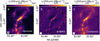 |
Fig. 1 G208 with Herschel and ArTéMiS. (a) Herschel 350 μm surface brightness map (Iℋ(350), resolution ≈ 20″); (b) ArTéMiS 350 μm surface brightness map; (c) The combined map obtained by feathering (Iℱ(350)). The beam is shown in the lower left corner of each image. The resolution of images (b) and (c) is around 10″. |
2.2 SED and MBB fitting
To estimate the dust (color) temperatures, Herschel 160–500 µm observations were fit with a modified blackbody spectrum:
 (1)
(1)
where Bν is the blackbody function and Iν the intensity at frequency ν, ν0 is a reference frequency, and β is the assumed value of the dust opacity spectral index. Equation (1) assumes that the emission is optically thin, as is the case in our fields with the possible exception of some dense cores at scales below the resolution of our data. We convolved the data using the convolution kernels provided in Aniano et al. (2011).
A least-squares fit was performed on each pixel separately and from this fit, we derived the dust temperature. The column density N(H2) was calculated from the obtained temperature via
 (2)
(2)
where Iν is the fitted intensity at frequency ν, μ = 2.8 is the mean molecular weight per free particle, mH is the mass of a Hydrogen molecule, and dust opacity κ is calculated as  (Beckwith et al. 1990), where we use β = 1.8, consistent with values found in many dense clouds (Juvela et al. 2015) and observed to be accurate for OMC-3 (Sadavoy et al. 2016).
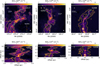 |
Fig. 2 Extracted filaments on the Herschel column density maps. Top row: Column density images (FWHM = 20″) of fields G17, G202, and G208 showing the extracted filaments in each field. Filament quality is marked by color of symbols: q = 1 (yellow circles), q = 2 (purple circles), q = 3 (orange crosses), and q = 4 (green crosses). The yellow contour shows the limit of AV = 3 mag. Bottom row: Extracted filament profiles, in which the filament center is at the center of the image. |
2.3 High-resolution N(H2) maps
To perform blackbody fits, we must normally convolve and reproject the data to the lowest resolution (in our case: Herschel PLW at ~35″). We instead calculated the column density maps at 20′′ resolution following the method described in Palmeirim et al. (2013). With this method, the column density at the resolution of the 250 µm observations can be calculated using the Herschel bands from 160 µm up to the wavelength indicated by the sub-indices of N(H2). In the following, an arrow refers to convolution to a certain full width at half maximum (FWHM); for instance, N (H2)350→500 is the convolution of a column density map derived using 160–350 µm, convolved to the resolution of 500 µm. This equation is expressed as:
 (3)
(3)
For further details, we refer to Appendix A of Palmeirim et al. (2013). Using the 350 µm feathered intensity map (Fig. 1c) and temperatures estimated from Herschel data, we calculated the column density for the feathered map using Eq. (2).
In this paper, we refer to the column density Herschel-only G208 map with the symbol NH and to the feathered G208 map with the symbol Nℱ. The 350 µm intensity maps are marked with Iℋ (350) and Iℱ (350), respectively. The final resolution of the feathered map is 10″, and the resolution of the Herschel column density maps are 20″.
2.4 Dense clump detection
According to Jeans’ criterion, a self-gravitating clump is believed to fragment into cores of mass

and size

where G is the gravitational constant, ρeff is the volume density, and the effective sound speed ceff is replaced by the total velocity dispersion  (Palau et al. 2014; Wang et al. 2014). The nonthermal velocity dispersion σNT is found from molecular line observations,while the thermal velocity is described by
  . Here, kB is the Boltzmann constant and Tkin the kinetic temperature. We assume dust temperature and kinetic temperature are similar, as is the case in regions with density of nH ≥ 105 (Goldsmith 2001). For a dust temperature of 20 K, similar to G208, the thermal component is σTH ≈ 0.27 km s−1. The temperature for each substructure is calculated as the median of all pixels within the substructure. The density, ρeff, is estimated assuming the clump is a sphere with a radius of
  , where rmax and rmin are the clump major and minor axes.
Suri et al. (2019) analyzed Orion A in C18O in the CARMA- NRO Orion Survey (resolution 8″). From Fig. 1 of their paper, we estimated the velocity dispersion in OMC-3 to be ~0.6– 0.8 km s−1, rising to ~1.2–1.4 km s−1 in the southern bright clump. We assume σNT ~ 0.8 km s−1 in the center of the filament.
Filament properties.
2.5 Filament analysis
The main filaments in each field were traced in the column density maps by eye. The filament profiles (perpendicular to the local filament direction) were extracted at even steps corresponding to one beam, 20″ in the case of Herschel column densities and 8.5″ in the case of the NF map. Each field has between 50 and 150 extracted profiles, depending on filament length (Table 2). The filament paths are shown in Fig. 2. The subfilaments in G17 and G202 complicate the filament selection. We related the extinction to the column density via N(H2)/Av = 1021 cm−2 mag−1 (Sadavoy et al. 2012) and we used a threshold extinction of Av = 3mag to eliminate background emission when calculating filament line masses. This Av ≥ 3 mask is twice the mean extinction of the background in G208 Nℋ and larger than the standard deviation in all fields. The Av < 3 component is not omitted during radial profile fitting.
The radial profiles of filament column density are generally well-represented by a Plummer-like function (Arzoumanian et al. 2011; André et al. 2014). We modified this function to include a linear background and convolved the model profile according to the angular resolution of the observed data,
![Mathematical equation: $Y = {\mathop{\rm Conv}\nolimits} \left[ {{N_0}\cdot{{\left( {1.0 + {{\left( {\frac{{r + \Delta r}}{{{R_{{\rm{flat }}}}}}} \right)}^2}} \right)}^{0.5 - 0.5\,\cdotp}}} \right] + a + b\cdotr,$](/articles/aa/full_html/2025/03/aa46425-23/aa46425-23-eq10.png) (4)
(4)
where r is the offset from the filament center, N0 is the filament’s central column density, Rflat the radius of the flat inner region, and p is the asymptotic power-law exponent. The term ∆r allows the center of the fitted filament to shift to better match the observations when the filament is not perfectly centered on the path that was traced by eye.
We also fit the profiles with asymmetric models, where the two sides of the filament have independent Rflat and p parameters, although based on the assumption of the same values of a and b on both sides of the filament. Unless otherwise noted, the results refer to the asymmetric fits. The effects of noise, sky background, background component model, distance to the source, fitting area, and convolution are explored in Appendix A.
The Plummer Rflat and p parameters give the FWHM of the fitted profile:
 (5)
(5)
which is more robust compared to the individual values of Rflat and p due to their partial degeneracy.
We calculated, for each profile, a S/N value by dividing the peak value of the filament segment with the noise level obtained from a region with the lowest emission (Table B.2). Profiles were assigned quality flags from q = 1 in the highest S/N quartile to q = 4 in the lowest S/N quartile. Individual profiles with poor quality flags (q > 2) were rejected from further analysis. We used quartiles as opposed to direct S/N values so that we could have different qualities within each field, with a sufficient number of datapoints to facilitate subsequent comparisons.
3 Results
In the following section, we first present general filament properties such as line masses and profile asymmetry. We then focus on Plummer profile fitting and compare the results derived for Nℋ and Nℱ data. Finally, we analyze the fragmentation of the regions by studying clumps and cores, along with a wavelet analysis.
3.1 Filament properties
Lengths of the filament spines and filament masses are listed in Table 2. The total filament mass is calculated using the pixels within the Av ≥ 3 mask:
 (6)
(6)
where N(H2)i,j is the column density and ∆x is the physical size of the pixel. The line mass (or mass per length) was then estimated as the average over the filament after the removal of the background. Using this criterion, G202 has a low line mass of 103 M⊙ pc−1 , whereas other filament sections have line masses above 150 M⊙ pc−1 . To accurately compare Nℱ and Nℋ filament properties, we include Nℋ,crop, the G208 Nℋ field cropped to the size of the Nℱ map. Mean N (H2 ) is the same within the Nℱ and Nℋ,crop maps, although of the two Nℱ has a higher maximum N (H2). This is due to the higher resolution of the Nℱ map, where the same high density is more diluted in the Nℋ,crop map.
Global gravitational stability of a filament can be estimated using the critical line mass of an isothermal filament (Ostriker 1964):
 (7)
(7)
where σTH is the 1D thermal velocity dispersion (defined in Sect. 2.4) and G is the gravitational constant. Temperature used to calculate σTH is the median over the Av ≥ 3 region. We first assume the full filament is thermally supported and, thus, we use only thermal velocity dispersion. At T ~ 20 K, the critical line masses are around 30–40 M⊙ pc−1, demonstrating that all the filaments are gravitationally unstable without support from magnetic or turbulent energy.
Again, we used C18O velocity dispersion from Suri et al. (2019) to estimate σNT (Fiege & Pudritz 2000) for G208, taking for the full OMC-3 region a value of σNT ~ 0.6 km s−1. Montillaud et al. (2019b) studied G202 in several molecular lines and so, we could estimate σNT ~ 0.7 km s−1 from their C18 O data for the region corresponding to our filament. For G17, we assume a similar value, σNT ~ 0.7 km s−1, due to the lack of molecular line data for the region. Critical line masses, M1,crit,TH+NT, now range from 200 to 270 M⊙ pc−2. G17, the full G208 Nℋ field, and the NF map have line masses that are greater than critical line mass, but with the addition of turbulent support the other fields may be gravitationally stable. However, we note that the estimate for G17 is only a general estimate.
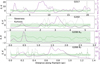 |
Fig. 3 Skewness (green dashed line) and kurtosis (gray dash-dotted line) along the filament spine of G17, G202, and G208 Nℋ and Nℱ. The right-hand y-axis shows column density along the filament spine (purple solid line). The faint gray horizontal line marks K = S = 0. S which falls outside of the green highlighted region is significant (see Sect. 4.2.1). |
3.2 Filament skewness and kurtosis
We plot Fisher-Pearson coefficient of skewness, S, Fisher kurtosis, K, and N(H2) along the filament spine in Fig. 3. The column density is computed as the mean of the pixels in a 3 × 3 grid surrounding the spine center, with pixel sizes for Nℱ and Nℋ being 0.76” and 6”, respectively. Then, S and K are calculated from the Plummer fits, from which we have subtracted the linear background; S describes the direction of the asymmetry of the filament, where a positive S indicates a left-leaning profile with a stronger tail to the right (i.e., leaning toward the positive RA axis). Skewness is calculated as8
 (8)
(8)
![Mathematical equation: ${m_{\rm{i}}} = \frac{1}{N}\sum\limits_{n = 1}^N {{{(x[n] - \bar x)}^i}} ,$](/articles/aa/full_html/2025/03/aa46425-23/aa46425-23-eq15.png) (9)
(9)
where mi is the biased sample ith central moment and  is the sample mean; K describes the shape of the profile compared to a Gaussian; therefore, a higher K describes a filament with stronger tails, while a Gaussian has K = 0. Kurtosis is calculated as9
 (10)
(10)
where μ4 is the fourth central moment and σ the standard deviation. Pearson correlation coefficients between column density, skewness, and kurtosis are shown in Table 4.
For a test sample of 1000 numpy random normal distributions of 1000 values each, mean values are (S) = −0.002 ± 0.08, 〈K〉 = −0.03 ± 0.15. In comparison, we list mean values from our data in Table 3. The 1-σ spread in S is consistent with a normal distribution in G208 Nℋ and Nℋ,crop, but slightly higher in other fields. G17 and G202 show negative S, G208 Nℱ positive. G17 and G202 show strong tails (i.e., a high K) when compared to a Gaussian, but this difference is less significant in G208 Nℱ. There is no statistically significant correlation between N(H2) and S or K. The high peak in K in G208 Nℱ corresponds to the region of highest column density.
Mean and 1-σ standard deviation of S and K in the fields.
Pearson correlation coefficients between column density, skewness, S, and kurtosis, K.
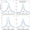 |
Fig. 4 Filament profiles in G17 (a), G202 (b), G208 Nℋ (c), and G208 Nℱ (d). The median filament profile is shown with solid lines, for quality 1 filaments (blue) and quality 1 and 2 (purple) profiles. The dash-dotted line shows the Plummer fit to the median filament profile. The dotted line shows the median Plummer profile, by taking the median of each individual Plummer parameter calculated. |
3.3 Plummer fitting
Filament column density profiles were fitted with the Plummer model. We plot the median profiles for each quality bin and the derived Plummer model in Fig. 4 for asymmetric fits. Plummer profiles are fitted out to 10′, which corresponds to r ~ 5 pc, 2 pc, and 1 pc from filament center for fields G17, G202, and G208 Nℋ, respectively. Due to the smaller extent of the ArTéMiS map, it can only be fitted to a distance of 1.3′ from filament center (~0.16 pc). For comparison with Nℱ data, we also fit the Nℋ data to the same extent and refer to this also as Nℋ,crop. Median derived plummer values are shown in Appendix D.
We derived mean FWHM values of 0.1–1.0 pc for asymmetric q = 1 fits using the three Herschel fields, but only ~0.05 pc using G208 Nℱ data. Power-law exponent of the Plummer profile, p, is generally below 5. We further compare G208 Nℋ,crop and NF fits in the next section.
Figure 5 shows the fitted FWHM values as the function of the field distance (frame a) and observational resolution in parsecs (frame b) for all three Herschel fields and the Nℱ map. When including only the Herschel filament profiles of quality 1 and 2, we derive a relation between distance in kpc and FWHM in parsecs of:

then, including ArTéMiS and all Herschel data, we obtain a relation between instrumental resolution HPBW and FWHM of:
![Mathematical equation: $FWH{M_{\langle q = 1 + 2\rangle }} \approx 6.7 \times HPBW[{\rm{pc}}],$](/articles/aa/full_html/2025/03/aa46425-23/aa46425-23-eq19.png)
where HPBW and FWHM are in pc.
We see a dependence of FWHM on distance and spatial resolution in our data, slightly steeper than the 4 × HPBW relation proposed by Panopoulou et al. (2022). Our fit is based on only four maps (including two observations of the G208 field), which is not sufficient to draw any universal conclusions. A correlation between distance or spatial resolution and derived FWHM is also seen in the literature, albeit with a more shallow slope than what we observe. In Fig. 5 we include Herschel continuum observations from Palmeirim et al. (2013); Schisano et al. (2014); Zhang et al. (2020); André et al. (2022); Zhang et al. (2022); Li et al. (2023), and continuum observations using other telescopes from Hill et al. (2012); Salji et al. (2015); Federrath et al. (2016); Kainulainen et al. (2016); Howard et al. (2019); Zavagno et al. (2020); Schuller et al. (2021). Although continuum and molecular lines do not necessarily trace the same filament, we included CO observations from Zheng et al. (2021); Guo et al. (2022); Yamada et al. (2022) and NH3 observations from Chen et al. (2022) in the right-hand frame. The FWHM values estimated with continuum observations (yellow and orange markers in Fig. 5) seem to follow the 2 × HPBW relation. Tentatively, it appears that in continuum observations FWHM converges to a value of ~0.05–0.1 pc when the resolution is better than 0.3 pc. Testing this possible convergence would require a larger sample of data at high resolution.
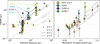 |
Fig. 5 Observed dependence of FWHM on filament distance and observational resolution. Left: FWHM from asymmetric fits plotted against the distance of the field of each q = 1–2 profile (squares and crosses, respectively). For readability, the distance values include small added jitter. Median of each distribution is plotted with a solid line (q = 1) and dashed line (q = 2). Grey lines show the proposed relation of FWHM = 4 × HPBW (Panopoulou et al. 2022), as well as the Herschel (solid line) and ArTéMiS (dashed line) beamsizes. Right: Median value of each q = 1–2 dataset as a function of observational resolution in pc (solid squares). The errorbars represent the standard deviation of the FWHM widths in each dataset. Grey lines show relations of FWHM = [1,2,4] × HPBW. In both frames, we also include values from the literature (see text for references): Herschel continuum (yellow triangles), other continuum (orange diamonds), mean deconvolved filament widths from Fig. 1 of Panopoulou et al. (2022) (yellow circles), and values from Juvela & Mannfors (2023) with solid plusses (LR and HR in yellow, AR with orange, and MIR with red). The errorbars represent either the published uncertainty or a 30% uncertainty on the FWHM. In the left frame only, we show additional literature values from CO (purple stars) and NH3 (purple hexagon) observations. Solid symbols represents deconvolved widths, those without beam deconvolution are shown with outlines. |
3.4 Comparing Plummer FWHM and column density
The FWHM values for each q = 1–2 filament profile are plotted against N(H2) in Fig. 6. The Pearson correlation was calculated between these two parameters, while the r- and p-values are listed in Table 5. In q = 1 profiles, significant correlation is found in G17 and G208 Nℋ . In the q = 2 profiles, correlation is generally not significant. This is possibly caused by low column density profiles, whereby the fits can return high FWHM values depending on background fluctuations. However, as we study only q = 1–2 profiles, column density in these cases is significantly higher than the background. In fits with Plummer p ≤ 10, correlation is less significant, due in part to the lower number of datapoints. When including only those profiles with p ≤ 10 in G202, we detect a (non-significant) anticorrelation between FWHM and N(H2); conversely by including all profiles field G202 shows a positive correlation.
3.5 Comparison between Nℱ and Nℋ in field G208
We plot the mean asymmetric Plummer profiles and the distributions of Rflat, p, and FWHM in Fig. 7, using the Nℱ and Nℋ,crop maps. T-tests comparing the two sets are shown in Table 6. The differences in FWHM, Rflat and p are all significant. Fitting the Plummer profile to the Nℋ,crop map, using the ArTéMiS pixel size, results in higher values of p, but also lower FWHM than by fitting the full NH map. However, restricting our analysis to those profiles with p ≤ 5.0 results in average FWHM values of 0.10 ± 0.01 and 0.05 ± 0.02 for Nℋ,crop and Nℱ, respectively.
Column densities using Nℋ and Nℱ data along the filament crest are shown in Fig. 8. There is difference of about 30% in column densities, consistent with the ArTéMiS calibration uncertainty.
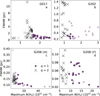 |
Fig. 6 Plummer FWHM plotted against the column density at the filament spine for Herschel fields G17 (a), G202 (b), and G208 (c), and the Nℱ map (d), for filaments of quality 1 (purple circles) and 2 (black crosses). Transparent symbols show profiles for which p > 10. |
Pearson correlation coefficients between Plummer FWHM and peak column density.
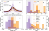 |
Fig. 7 Comparison of G208 Nℱ and Nℋ,crop filament shapes. Frame a: Profiles of Nℋ (orange) and Nℱ (purple) q = 1–2 filaments. Median profiles are plotted with solid and dashed lines for q = 1 and q = 2 profiles, respectively. Frames b-d: histograms of p (b), Rflat (d), and FWHM (c) for all q = 1–2 filaments in field G208. Medians and means for each distributions are plotted in dashed and dotted lines, respectively. The shaded areas correspond to the central 1-σ regions of the distributions. |
3.6 Fragmentation
We study fragmentation of the filaments in G208 using wavelet decomposition as well as by using the extracted clumps. In this analysis, the noisy edges are removed from the NF map and we use the Nℋ,crop map (Fig. 9).
T-test results between Plummer parameters computed for G208 Nℋ,crop and Nℱ.
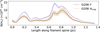 |
Fig. 8 Comparison of derived N(H2) in G208. N(H2) along the filament crest for the Nℱ (purple dashed line) and Nℋ,crop (orange solid line). The Nℋ,crop map is at 20″ resolution, and Nℱ has been convolved to the same 20′′ resolution. |
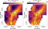 |
Fig. 9 Clump ellipses (cyan) plotted on top of the Nℋ,crop (left) and Nℱ (right) column density maps. The three clumps removed from analysis are drawn with white outlines on the Nℱ map. The orange circle shows the region used for determining the RMS noise. |
3.6.1 Clumps
Dense clumps were identified in the Nℱ and Nℋ,crop column density maps using the astrodendro package10 (Goodman et al. 2009). The dendrogram algorithm describes the data as a hierarchy of structures of progressively smaller size. In order to find the densest clumps, we use the leaves of the dendrogram. We require fitted structures have a minimum column density of 2 × RMS, where RMS is the standard deviation within a relatively empty region (the orange circle in Fig. 9). Five clumps are found in the Nℋ,crop map and sixteen in the Nℱ, although three of the NF clumps are likely due to noise at the map edges and are excluded from further analysis. The ellipses for these clumps are shown in Fig. 9 and their properties are compared in Fig. 10 and Table 7.
Notes. Dust temperature, column density, clump radius, and clump mass (columns 1–4) are estimated from MBB fits to Herschel 160–500µm data. Effective radius is calculated as  , where a and b are the clump major and minor axes. Columns 5-6 list the effective Jeans’ length λj and effective Jeans’ mass MJ, where non-thermal velocity dispersion is estimated from Suri et al. (2019), ⟨σ NT⟩ ≈ 0.8 km s−1. Due to the similar mean temperatures, (σ TH) = 0.24 km s−1 and ⟨σtot⟩ = 0.83 km s−1 for both Nℱ and Nℋ,crop clumps. Column 7 lists the average mass surface density and column 8 gives the mean separation between neighboring clumps (s).
Even though the Nℱ clumps are smaller, they have a higher median N(H2) and mass per area; however, the derived clump mass is generally lower than Jeans mass. Figure 11 shows the spectral energy distributions (SEDs) of the four densest clumps in each field from 160 to 500 µm. Based on MBB fits assuming constant β = 1.8, clumps in all but G202 are generally warm, at T ~ 18–20 K.
We calculated the distances between the clumps. The mean separation is (0.28 ± 0.14) pc for the Nℋ,crop map and (0.13 ± 0.06) pc for the Nℱ. The mean clump separation in the Nℱ map is close to the estimated effective Jeans length of 0.1 pc, while a mean separation in the Nℋ,crop map is approximately double the effective Jeans length. It is therefore likely that many of the clumps in OMC-3 are gravitationally unstable with the possibility for future star-formation.
We searched for YSOs from the Megeath et al. (2012) Spitzer catalog, finding 23 YSOs that overlap with the Nℋ,crop clumps. Of these, Megeath et al. (2012) classified nine as D-class (or premain sequence stars with a disk). The rest are classified as Pclass, or protostars. Ten of these YSOs also overlap with clumps in the Nℱ map, with all six classified as protostars. All Nℋ,crop clumps are spatially associated with at least one YSO.
Clump profiles in the column density maps were fitted with power-laws r–α following the methodology of Shirley et al. (2000). We derive mean major-axis power-law indices of α = 1.54 ± 0.96 for G208 Nℋ,crop, and α = 1.21 ± 0.74 for G208 Nℱ. Minor-axis power-law indices are smaller, with 0.97 ± 0.59 for Nℋ,crop and 0.75 ± 0.69 for Nℱ.
Clump characteristics in G208.
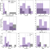 |
Fig. 10 Comparison of clump properties found in Nℋ,crop (gray) and Nℱ (purple dotted) column density maps. The corresponding median values are plotted with gray dashed and purple dash-dotted lines for Nℋ,crop and Nℱ, respectively. |
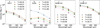 |
Fig. 11 SEDs of the four brightest clumps in each field, at 160–500 µm. The dashed lines represent MBB fits with constant β =1.8 for each clump. The best-fit temperature for each clump is listed in the legend. |
3.6.2 Wavelet decomposition
We performed wavelet filtering to identify structures at various spatial scales, as in Mattern et al. (2018). The column density maps are decomposed into scale maps Xi at scales from 0.01– 0.4 pc, where we require that the minimum scale used is larger than the pixel size of the image. The maximum scale used is the scale at which no distinct structures are visible in the map after convolution. For this analysis, we have focused only on the Av ≥ 3mag regions. We require that each structure at level i overlaps with a structure at levels i + 1 and i – 1. At the lowest and highest levels, we require the structure to only overlap at levels i + 1 or i – 1, respectively. This method is explained in detail in Kainulainen et al. (2014). We then find clumps in these decomposed images using Dendrograms, taking each leaf as an individual structure. Derived properties of these structures are listed in Table B.6. Mass of each structure is calculated with

where ⟨N(H2⟩ is the mean N(H2) of the region, calculated as the mean over all pixels in the clump footprint, Ω the solid angle, d the distance, and μmH the mass of the Hydrogen molecule. Hydrogen number density nH is
 (11)
(11)
where a and b are the major and minor axes of the structure, V is the volume of the structure, assuming a prolate spheroid shape,  . We calculate median separation s between substructures.
Not surprisingly, the number of structures increases toward smaller scales, though not in a linear fashion. Though the total mass increases with spatial scale, the highest masses are around scales of 3.0, 1.0, and 0.75 pc for G17, G202, and G208, respectively. This may simply be due to the smaller number of structures at the largest scales. Both mean volume and column densities decrease toward larger scales, not surprising as more of the diffuse ISM is included in the structures. In G208, Nℋ N(H2) is at its peak at scales of 0.05 pc. In G208, Nℱ is the median separation between structures in all but the largest two levels, which is smaller than the Jeans length; whereas in the Nℋ G208 field, median separations are all larger.
4 Discussion
4.1 Cloud properties
The Herschel Gould Belt survey has observed a range of nearby star-forming regions, with filament line masses in the range 1– 204M⊙ pc−1 (Arzoumanian et al. 2011; Palmeirim et al. 2013; Arzoumanian et al. 2019). We found similar line masses in all fields. Quiescent clouds generally have lower line masses, such as those observed with CO molecular line transitions in the Perseus MC (Guo et al. 2022) or the quiescent Musca cloud (Kainulainen et al. 2016), or for a sample of nearby (d < 500 pc) filaments imaged with Herschel (Arzoumanian et al. 2019). We derived line masses of ~ 170-300 M⊙ pc−1 in OMC-3, similar to those derived by Schuller et al. (2021) and Li et al. (2022), also for OMC-3. Similar line masses were also derived in the high-mass SF region G345.51+0.84 with ALMA and Herschel (Pan et al. 2023) and in extragalactic sources, such as the N159W-North filament in the Large Magellanic Cloud (LMC) observed with ALMA (Tokuda et al. 2022). Our derived line masses of 100-300 M⊙ pc−1 (Table 2) are under half of that derived for the Nessie filament (Mattern et al. 2018) and a fifth of those derived for a sample of large-scale filaments within the ATLASGAL survey (Ge & Wang 2022).
Our derived column densities for G208 Nℋ, with maximum N(H2) over 1023 cm−2, are similar to that of Schuller et al. (2021) (Fig. 12). Within the densest regions of the filament, the column densities derived by Schuller et al. (2021) are higher by up to 1023 cm−2, corresponding to a difference of 56% in the total column density. The differences in derived N(H2) are likely due to two factors: calibration uncertainty and different feathering methods used in this work and in Schuller et al. (2021), as well as a different combination of maps used to derive the temperature and column density. The significantly higher column densities in the Schuller et al. (2021) map correspond to dense cores, which also have higher surface brightness than in our data (Fig. 1 in Schuller et al. (2021) compared to Fig. 1 in this paper). Similar column densities to those in G208 have been detected in a sample of 11 IRDCs and in the high-mass star-forming NGC 6334 complex using Herschel and ArTéMiS data (André et al. 2016; Peretto et al. 2020). Column densities of ~2 ×1022 cm−2 have been observed in two IRDCs using ArTéMiS, LABOCA11, and Herschel data (Miettinen et al. 2022). Slightly higher column densities of ~5 ×1022 cm−2 were observed using ArTéMiS and Herschel SPIRE/HOBYS data of the Galactic H II region RCW 120 (Zavagno et al. 2020), similar to the mean values over the whole G208 filament.
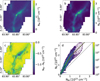 |
Fig. 12 Comparison between column densities derived in this work (NM) and in Schuller et al. (2021) (NS) using a combinations of Herschel and ArTéMiS observations. Frame a: This work. Frame b: Schuller et al. (2021), APEX project 098.F-9304. Frame c: Difference between this work and that of Schuller. The contours correspond to NM = (0, 0.25, 0.5, 1.0) × 1023 cm−2 Frame d: Comparison plot between N(H2) values. The black dashed line represents a 1–1 relation, while the colored lines give the linear fits between NM and NS, with colors corresponding to the contours in frame c. |
Skewness and kurtosis calculated for simulated filaments with the symmetric Plummer parameters of our q = 1 profiles.
4.2 Plummer fitting
4.2.1 Symmetry of the filaments
To study what the normal values of skewness (S) and kurtosis (K) are, we simulated filaments with the symmetric Plummer parameters of our q = 1 filament segments (listed in Table D.2). We included a power-law background and an additional Gaussian large-scale component to simulate hierarchical structure. Asymmetric Plummer fits were performed on these simulated filaments and from a total of 1280 filament profiles, we calculated the mean S and K. As the generated filament profiles are symmetric, the values in Table 8 give lower limits of S which correspond to significant asymmetry.
When comparing the derived values of S (Table 3), all filaments have mean values lower than the limits set by the simulation. However, as seen in Fig. 3, G202 and G208 Nℱ have regions where the skewness is outside of these limits. Strong external directional forces (e.g., from SF) are likely to affect the OMC-3 filament. Zheng et al. (2021) also found an abundance of asymmetric filaments within the Orion A cloud with CO observations, with most filament segments in OMC-3 being asymmetric in their paper. Likewise, Peretto et al. (2012) found multiple asymmetric filament profiles in the Pipe nebula using Herschel observations, which they interpreted as being due to compression flows from the Sco OB2 association. The multiple filament segments and colliding filaments in G17 and G202 are also likely to raise S in these filaments and it is unclear whether the segments of significant asymmetry in these two filaments are caused by external forces or filament collision.
4.2.2 Filament widths
We found mean filament FWHM widths of ~1.0, 0.3, 0.1, 0.08, and 0.05pc for fields G17, G202, G208 Nℋ, G208 Nℋ,crop, and G208 Nℱ, respectively. As shown in Fig. 5, the distance to the field and instrumental resolution seem to affect derived width. This is likely due to the increasing resolution of nearer fields: at larger distances, the observed filament includes more of the extended structure. Juvela et al. (2012) found that at the nominal Herschel resolution, assuming 0.1 pc widths, the filament parameters could be recovered reliably only up to a distance of 400 pc. In the future, the ArTéMiS resolution is expected to double this threshold. A dependence on distance has been found in multiple studies (Rivera-Ingraham et al. 2016; Panopoulou et al. 2022; André et al. 2022). Panopoulou et al. (2022) suggested a relation between distance of FWHMfilament ≈ 4 × HPBW, shallower than that that found among our sample, but steeper than a fit to continuum FWHM values from Fig. 5, which gives a relation of FWHM ≈ 1.8 × HPBW. André et al. (2022) also find a slight dependence between distance and width, suggesting that a characteristic width exists, but that it is unresolved at distances > 1 kpc.
Molecular line observations from the literature also show a potential correlation between resolution and FWHM although molecular lines do not necessarily trace the same filaments as continuum data. Simulations by Priestley & Whitworth (2020) find that filaments detected in CO are several times larger than the same filaments detected in continuum observations, but narrower when detected using dense gas tracers such as HCN and N2H+. Observations of the Orion regions show a similar discrepancy between molecular line and continuum observations (Shimajiri et al. 2023). Furthermore, slightly different fitting processes (including the level of background subtraction, deconvolution, and filament extraction methods) can affect the derived filament widths.
Although G208 Nℋ shows the characteristic 0.1 pc width, the same field observed with the resolution of ArTéMiS shows widths of only ∼0.05 pc. This is similar to results found by Smith et al. (2016), Schuller et al. (2021), and Panopoulou et al. (2022). Due to the multiscale nature of the dense ISM, it is not surprising that filament-like structures can be observed at many scales. Though dense fibers have been detected in the Southern OMC-3 region in N2H+ (Hacar et al. 2018), further high-resolution continuum data are needed to quantify the internal structure of filaments at the scale of the fibers. While fibers are not visible in the MIR extinction data of Juvela & Mannfors (2023), these observations are limited by 8 µm absorption saturating toward the densest filaments. Schuller et al. (2021) compared their observations with those of Hacar et al. (2018). They found that while N2H+ generally seems to correlate with the densest region of the filaments visible in the continuum, N2H+ can be destroyed by interactions with CO and by high-energy radiation. This can narrow filament profiles observed with molecular lines.
André et al. (2022) suggested that the apparent relation of distance to FWHM can be mostly explained due to the convolution of a Plummer-like filament combined with background noise fluctuations. However, assuming an intrinsic width of 0.1 pc, the mean FWHM values of G202 should be only ∼0.13 pc according to their Figure 3b.
This conclusion certainly depends also on the relative strengths of the background components and the filament, as well as on the sizes of the background fluctuations. The powerlaw exponent of the background fluctuations in the full Herschel fields is around -2, shallower than that found in Herschel SPIRE observations of the Polaris Flare (Miville-Deschênes et al. 2010). However, Miville-Deschênes et al. (2010) have both a larger map size, as well as lower resolution of ∼30′′, possibly explaining this difference in power-law exponent. Whether the background is described by an exponent of –2 or –3 does not significantly affect the derived filament’s FWHM. Performing the simulations in Appendix A.3, using a modeled background with a powerlaw slope of −2, results in FWHM values of 22.3 ± 5.5 pixels; assuming a slope of −3, we derived a result of FWHM = 25.1 ± 10.4 pixels, which is in agreement within the uncertainties. Both power-law backgrounds increase the derived FWHM from the original value of 20.78 pixels.
The relative strengths of the background components are difficult to identify and they depend on the positions of the filament segment in relation to the wider cloud. Comparing the standard deviation across the whole background (defined as the Av < 3.0mag region) with the maximum intensity of each filament segment results in S/N values from 10–100. However, this method does not necessarily take into account all background structures, especially those on scales larger than the observations; thus, the “true” S/N may be lower than the calculated value. Simulations in Appendix A.2.1 show the effects of lower S/N on filament widths. Although the mean FWHM values do not significantly change, the uncertainty increases. Further simulations in Appendix A.3, which include a wide Gaussian component with an ideal narrow filament, result in FWHM values which increase by up to 30% at 2 kpc from the original width. Similar simulations not including this wide component result in an increase of FWHM of up to 10%. The S/N also affects derived widths by a further 5% if it is decreased from 100 to 10. These simulations reveal how large-scale structures can artificially widen filament profiles as well as how detected filament widths increase slightly as a function of distance, even if we are only studying an ideal narrow filament.
As the simulations of Appendix A.3 show, convolution and background fluctuations, combined with the multiscale nature of the ISM, will affect derived filament widths. The chosen definition of a filament further complicates analysis. In C18O data, Suri et al. (2019) find tens of filament segments in the OMC-3 region. By segmenting these data in another way, derived mean filament widths can change significantly.
In Juvela & Mannfors (2023), we have compared four of the densest filament segments using Herschel and ArTéMiS emission, as well as Spitzer extinction. When comparing only the dense filament segments, also Herschel data show a relatively low width of 0.05–0.1 pc. This differs significantly from the results derived across the entire OMC-3 filament and may be explained by the consistently high column densities of the filament profiles in Juvela & Mannfors (2023). In this present paper, FWHM is also lower in more dense filament segments. It seems that, when looking only at the regions of OMC-3 with the highest filament strength compared to the background, derived width does not depend on resolution. Whether this would hold in G17 or G202 is unknown. Furthermore, both the resolution (∼2″) and S/N in the mid-IR Spitzer data were higher than the ArTéMiS resolution and S/N.
A wide range of filament widths have been found in the literature. Using Herschel SPIRE observations for a sample of filaments, Schisano et al. (2014) found mean filament widths between 0.1–2.0 pc, increasing with distance to the filament. Using ArTéMiS and Herschel, Schuller et al. (2021) find similar widths to our NF field of 0.06 pc in OMC-3. Similar values of ∼0.07 pc are detected by Kainulainen et al. (2016) using dust extinction mapping. Various combinations of JCMT SCUBA-2, ArTéMiS, and Herschel data results in FWHM ∼0.08–0.12 pc (Hill et al. 2012; Salji et al. 2015; Howard et al. 2019; Zavagno et al. 2020). The FWHM values as high as 0.3 pc have been detected in the Vela C cloud at a distance of ∼900 pc (Li et al. 2023) using Herschel data alone. Similarly high values of 0.17 pc are detected in the central molecular zone at a distance of 8.3 kpc using ALMA and Herschel data (Federrath 2016).
4.2.3 Parameters p of the Plummer fits
Our derived median power-law indices using asymmetric fits are p ∼2–5, with some outliers reaching up to 25. However, values of p over 5 are unlikely to be accurate, and are probably due to the degeneracy between the Rflat and p values. Large values of p may be caused when a filament has a steep profile and the shape of the convolved profile is dominated by the convolution by the beam, as opposed to emission from the filament. In addition, Juvela & Mannfors (2023) found that dips in column density in profile tails can cause large values of p. However, large p values do not affect the shape of the derived profile. For example, the asymmetric fits to G202 and G208 NF in Fig. 14 both have fitted p = 25.
In symmetric fits to Herschel data, the median indices p are below 4. Values from the literature are generally lower, with p ∼ 2.0 ± 0.4 found in Taurus (Palmeirim et al. 2013), p ∼ 2.6 ± 11% in Musca (Kainulainen et al. 2016), p ∼ 2.2 ± 0.3 in a sample of nearby filaments (Arzoumanian et al. 2019), and p ∼ 1.5–2 in Hi-GAL filaments (André et al. 2022). Schuller et al. (2021) also reported p = 1.7–2.3 in OMC-3.
4.3 Comparison between feathered and Herschel-only fits
We found significant differences between NH and NF data. The FWHM values of the profiles is over two times larger in NH data, directly proportional to the data resolution. This is a difference of ∼(2–3)σ in q = 1–2 filaments. This is true for both symmetric and asymmetric fits. This difference is similar to that found recently by, for instance, Smith et al. (2016) and Panopoulou et al. (2022) as well as Schuller et al. (2021) in OMC-3. Fragmentation also shows increased substructure with the inclusion of higher-resolution ArTéMiS data, both through clump detection and wavelet analysis. With even higher resolution data, such as those from ALMA or JWST, smaller cores and fibers could possibly be detected.
4.4 Comparison of various Plummer fitting methods
In the following, we study how the results depend on different methods of Plummer fitting. We compared fits using symmetric and asymmetric Plummer functions, examine the differences between the fits to individual filament cross sections and to the mean filament profile. Finally, we study how adding the offset ∆r to the Plummer formula (Eq. (4)) would change the results.
4.4.1 Symmetric and asymmetric fits
Although we used asymmetric Plummer fits in our study, Fig. 13 shows a comparison to symmetric fits. In a symmetric fit, both sides of the Plummer function have the same Rflat and p values. What is especially noticeable is the spread in p for all but G208 Nℋ. As an example , we plot one q = 1 filament with the highest offset for each field in Fig. 14. Values for the fits, including χ2 values, are listed in Table 9.
Comparing the results of symmetric and asymmetric fits for our whole sample from Tables D.1–D.2, we see that they generally do not differ by more than 1σ. The median FWHM does not differ significantly between the two fits. Although the median FWHM of the G208 NH filaments is approximately 0.1 pc, neither the other fields nor the NF map display a characteristic width.
4.4.2 Analysis of the mean profile or analysis of multiple filament profiles
Many studies (e.g., Arzoumanian et al. 2011; Rivera-Ingraham et al. 2016) of filament widths concentrate on the analysis of the mean or median profile. We have compared fits to the median profile and the median of all the fits to individual cross sections in Fig. 15. Median values of p in G208 Nℱ are higher when estimated from the mean profile, but slightly lower in the Herschel fields. Rflat and FWHM are remarkably consistent, regardless of the fitting methods used. The correlation between the two fits is better in profiles of higher quality, which is not surprising as a stronger background or noise will introduce more uncertainty into the fits. A similar correlation (also with the inclusion of MIR data) was reported in Juvela & Mannfors (2023, as shown in Fig. 3d).
More information about the distribution of values is accessible by fitting individual profiles instead of just their average. As shown in Fig. D.1, the distribution of individual parameters may be quite wide, even at higher quality flags (q ≤ 2). In contrast, the parameter p is more robust when fitting to the median profile.
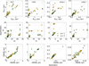 |
Fig. 13 Comparison of symmetric and asymmetric Plummer fits for all fields. Rflat (top row), p (middle), and FWHM (bottom row) for symmetric (x-axes) and asymmetric (y-axes) fits. The q = 1 profiles are plotted with yellow circles and q = 2 profiles with green triangles. The gray solid line shows a 1:1 relation and the gray dashed lines highlight the allowed upper and lower limits of the Plummer parameters. |
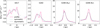 |
Fig. 14 Profiles of the q = 1 filament with the largest offset in each of the four fields. The pink solid line corresponds to the observed profile, the blue dotted line to the symmetric Plummer fit and the black dashed line to the asymmetric Plummer fit. |
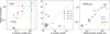 |
Fig. 15 Fit to the median profile plotted against (y-axis) the median values calculated separately for each filament profile (x-axis). The gray solid line represents a relation of y = x. Quality flags are represented by a star, square, circle, and triangle, in order of decreasing quality. The fit to the entire field, regardless of quality flag, is shown by an asterisk. The dashed lines represent upper and lower bounds to the fits. In frame 1, the color of the line corresponds to the field. |
4.4.3 Comparison of fits with and without offset
We compared the fits with and without ∆r, the parameter which allows the filament peak to shift. The FWHM calculated without the offset term is plotted against the FWHM derived using the offset in Fig. 16. All four fields show good correlation between the values for the q = 1–2 filaments, although generally the FWHM tends to be somewhat higher in fits with offset. Greater variation is seen in lower-quality filaments, especially in G17 and G208 Nℱ.
4.5 Clump powerlaws
We fit the clump profiles with powerlaws of r-α and found mean powerlaw indices of 〈α〉 = 1.21 ± 0.74 for G208 Nℱ, and 〈α〉 = 1.54 ± 0.96 for G208 Nℋ,crop. The Nℋ,crop values are similar to those found in an analysis of Class I and 0 protostellar cores using the SCUBA instrument at the James Clerk Maxwell Telescope (JCMT; Shirley et al. 2000, 〈α〉 = 1.48 ± 0.35), whereas the Nℱ clumps are somewhat shallower.
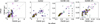 |
Fig. 16 FWHM values for all four datasets, calculated using the Plummer formula (Eq. (4)) with no term for offset (x-axis) and including ∆r (y-axis). The gray line plots a 1:1 relation. |
4.6 Fragmentation length
We estimated effective Jeans lengths of ~0.1pc in G208, similar to the typical width for interstellar filaments, consistent with Arzoumanian et al. (2013). The median separation between dense clumps in the Nℱ map is also a similar distance, suggesting that thermal gravitational fragmentation is sufficient to explain the fragmentation at these scales.
As in Mattern et al. (2018), more structures are found at smaller spatial scales; however, in their paper, the largest number of clumps are found in the second scale. In our fields, all Herschel fields have a similar number of structures at the lowest two levels, whereas the G208 Nℱ displays more structures at level 1 (corresponding to 0.025 pc). It is not unexpected to see that the median column and volume densities decrease toward larger scales, as was also found in Nessie. However, the mean N(H2) in G208 Nℋ stays constant until ~0.5 pc, in G202 until 0.1 pc, and in G17 until ~0.5 pc, at scales larger than the beam size. In G208 Nℋ, the dependence between column density and spatial scale is approximately linear.
We did not detect fragmentation in G202 and G208 Nℋ above 1.0 pc. However, this is likely due to the limit of our map sizes, as opposed to a physical upper limit of fragmentation. In comparison, with a mapsize of 1° × 20″ at a distance of 3.5 kpc, Mattern et al. (2018) identified fragmentation on scales from 0.1– 10pc in Nessie. These larger fragmentation scales likely exist in our fields, but above the resolution of the data.
In our data, median separation s is negatively correlated with median density. A similar anticorrelation is detected in Mattern et al. (2018), although OMC-3 has higher densities by a factor of 102 compared to Nessie. Palau et al. (2014) have also observed an increase of fragmentation (which would lead to smaller separation) with a higher density. The slope of the Mattern et al. (2018) relation matches that found in G17 and G202. Orion shows a steeper relation between density and s. The mean separation between substructures in all but G208 Nℱ is larger on all scales apart from the Jeans length. In Nℱ the mean separation is under 0.1 pc at scales below 0.05 pc. Both the analysis of dense clumps as well as wavelet decomposition show increased fragmentation at the ArTéMiS resolution.
4.7 Parameter uncertainties
Due to uncertainties in the background, the Plummer fitting routine can fit the data with a range of parameter values. In order to study uncertainties due to the fitting routine, we performed a simulation of a filament plus a background sky that was generated based on a powerlaw power spectrum. We ran 100 fits to a map of size 100 × 100 pix (a total of 10 000 fits), calculating the mean, median, and standard deviation of the Plummer parameters. For each run, the random fluctuations of the sky varied, but the power-law index (k = –2) did not, and no white noise was added to the filament itself. The results of the runs are shown in Tables B.3 and B.4 for symmetric and asymmetric fits, respectively.
We found an uncertainty due to background fluctuations on Rflat of 4.0%, on p of 2.7%, and on FWHM of 3.6% for asymmetric fits. Uncertainty on symmetric fits is similar, at 4.2% and 2.5% for Rflat and p, respectively, but slightly lower (3.0%) for the FWHM.
We study the sources of errors in Plummer fitting further in Appendix A. As we include only those filament profiles with high quality flags in our analysis, the error due to S/N variations are not likely to be large. It is only in field G17 that the S/N is low enough to affect derived parameters (Table B.5). Simulations of varying background fluctuation strength show that uncertainty increases with a stronger sky; this too, should not be a problem in our sources. A stronger source of uncertainty can arise from large-scale structure similar to the large Gaussian structure in Appendix A.3, which can artificially widen the extracted filament by up to 30% at 2 kpc. This was discussed in more detail in Sect. 4.2.2. The model used to fit the filament background can affect derived parameters. In this paper, we assume a linear background. We have tested fits with a polynomial background in Appendix A.2.3, finding no significant difference between linear and polynomial background fits in OMC-3. The possibility of a strong background component can results in uncertainty up to 50% in terms of the FWHM.
The Plummer fits included 1D beam convolution as part of the fitting procedure. In Appendix A.5, we test this against the more correct way of convolving the predictions of the fitted model in 2D. In this case, the convolved values become dependent also on the neighboring filament cross sections. It is likely that the spread in derived Plummer values would decrease with the use of a 2D convolution; however, in regions with a distinct filament the difference between 1D and 2D convolution is small. Thus, in practice the difference between the 1D and 2D approaches does not cause significant differences in the parameter estimates.
Temperature variations along the line of sight can bias estimates of the opacity spectral index, β (Shetty et al. 2009; Malinen et al. 2011). The submillimeter κ and β are also dependent on the assumed sizes and optical properties of dust grains (Ormel et al. 2011). In the dense cores and filaments, the line-of- sight temperature variations combined with the uncertainty of the dust properties can cause the column densities to be underestimated by even up to a factor of ten (Malinen et al. 2011). Because these effects depend the column density, they can have systematic effects also on the filament profiles that are derived via modified blackbody fits. This will again have a greater effect on the individual profile parameters, while the FWHM estimates will be more robust (Juvela & Mannfors 2023).
5 Conclusions
We have analyzed the main OMC-3 filament using continuum Herschel (Nℋ) and ArTéMiS data. The Herschel and ArTéMiS data have been combined to provide a higher-resolution image (Nℱ). Filament morphology as well as fragmentation have been studied. We have further observed two other fields with Herschel, G17 and G202, located at larger distances of 1.8 kpc and 760 pc, respectively.
Line masses of the examined filaments are in the range 103– 310 M⊙ pc−2 . Assuming only thermal support, all filaments are gravitationally unstable. With the addition of turbulence, G202 and G208 Nℱ are stable against gravity. All filaments show some asymmetry, but only G202 and G208 NF has significant asymmetry across most of the filament.
The relation between filament FWHM and instrumental resolution can be fit with by FWHM ≈ 6.7 × HPBW [pc], suggesting that telescope resolution can affect derived properties. We also find an increase in FWHM with distance in simulated ideal filaments (Appendix A.3). However, in the densest filament segments of OMC-3 studied in Juvela & Mannfors (2023), with the highest signal relative to the background, filament FWHM is relatively independent of resolution.
We did not detect any significant correlation between filament FWHM and column density.
The widths of the Nℱ filaments in OMC-3 are ∼0.05 pc, half of the 0.1 pc typical width observed in many Herschel filaments. Meanwhile, the FWHM of Nℋ in OMC-3 filament segments is ∼0.1 pc. Hierarchical structure within the ISM will result in filament-like structures visible at many scales and may in part explain the dependence on the resolution of the observations. Further contributions to this relation likely come from convolution of large-scale structures within the ISM. Models show that large-scale fluctuations in the background can increase the derived FWHM.
Compared to Herschel, ArTéMiS probes denser structures, which have higher column density and mass per area but smaller physical size. Most of the clumps detected within OMC-3 are not gravitationally bound, with the exception of two dense clumps detected in the Nℱ map. The effective Jeans length in OMC-3 is ∼0.1 pc.
A higher number of structures are visible at small scales in the Nℱ map and the median separation of Nℱ structures at scales of ≤ 0.05 pc is below the Jeans length. On the NH map, the median separation between substructures at small scales is ~0.1–0.2 pc. Furthermore, the median separation for clumps detected in the Nℱ data of (0.1 ± 0.1) pc is within 1σ of the Jeans length, but Nℋ clumps display a median separation of 0.3 pc.
We analyzed how the derived Plummer parameters depend on the type of fitting procedure.
- (a)
Asymmetric fits, where the two sides of the filament profile are fit with different Rflat and p values were compared with symmetric fits. Mean values of the parameters do not generally differ by more than 1σ. Although individual Rflat and p parameters can have large variations (up to a factor of 2), the derived FWHM is fairly similar.
- (b)
Major differences in the Plummer parameters are not seen when fitting the mean filament profile, compared to fitting the individual filament cross sections. This difference increases in cases where the filament is weak compared to the background. Once again, FWHM is robust against changes in Rflat and p.
- (c)
Allowing the peak of the filament to shift along the x-axis results in a slightly higher FWHM. The effect is less than 20% in q = 1 filaments, but it can rise to almost a factor of 2 in low-quality filaments (q > 2).
- (a)
The complex nature of interstellar filaments and of the wider environment creates uncertainty in fitting of filament properties. Care must be taken when drawing conclusions from individual observations. Multiscale continuum observations of single filaments are crucial to untangling the effects of resolution from intrinsic properties.
Data availability
Appendices B and D are available on Zenodo.
Acknowledgements
E.M. was funded by the University of Helsinki doctoral school in particle physics and universe sciences (PAPU). E.M. is funded by the Vilho, Yrjö ja Kalle Väisälä Foundation of the Finnish Academy of Science and Letters. MJ acknowledges support from the Research council of Finland grant No. 348342. Software: APLpy (Robitaille & Bressert 2012), Matplotlib (Hunter 2007), Astropy (Astropy Collaboration 2013), Numpy (Harris et al. 2020), uvcombine, Montage (Berriman et al. 2004; Good & Berriman 2019), scipy (Virtanen et al. 2020).
Appendix A Simulations of Plummer fitting
We tested the accuracy of Plummer fitting and derived parameters by varying the S/N, background, and distance (and therefore resolution) of simulated filaments. The initial parameters used to create the Plummer profile in these simulations are listed in Table A.1.
Initial Plummer parameters used in these simulations.
A.1 S/N variation
Noise was added to the Plummer model using

where N (0,1) are normally distributed random numbers, and Y is the (symmetric) Plummer function (Eq. 4). We tested S/Ns of 2, 5, 10, 25, 50, and 100. This Plummer model was convolved using a 1-D convolution. We fit the Plummer function to Y0 using scipy’s leastsq function. The derived values of FWHM, R, and p are shown in Fig. A.1. Already at S/N 25 the least squares fitting routine recovers the Plummer filament well, with mean estimated FWHM being within 1% of the FWHM of the original profile.
A.2 Background variation
We tested the effect of the background on the derived Plummer model. In Sect. A.2.1, we test how the relative strength of the filament compared to the background sky affects derived Plummer parameters. In Sect. A.2.2 we compare Plummer fits to a simulated filament with a linear or polynomial background component, and in Sect. A.2.3 we test a polynomial fit on our four fields.
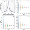 |
Fig. A.1 Effect of varying S/N on Plummer filament fitting. (a) Profile showing the original Plummer without noise (black plusses), the fit with S/N = 2 (black solid line), S/N = 5 (teal dotted line), and S/N = 10 (dash- dotted line). The simulated filament profile assuming S/N = 2 is plotted with faint gray. (b–d) violin plots of derived FWHM, R, and p with increasing S/N. The dotted line corresponds to the original Plummer parameter, R = 6.0 and p = 2.0. |
A.2.1 Fluctuations of the background sky
We studied the effect of background sky fluctuations on derived filamentary properties. We assumed that the background has a spatial power spectrum that is a powerlaw with an exponent of -2 (similar to the background powerlaw shape in OMC-3) and convolved it using a 2D convolution. We varied the ratio of the filament peak divided by rms value of the background fluctuations, calling this property S /Nfilament . The Plummer filament itself does not vary (except for the random effects due to white noise corresponding to S/N = 100, as presented in Sect. A.1). We fit the Plummer model using the same method as in Sect. A.1. Two resulting 1D profiles, along with background sky, are shown in Fig. A.2b–c, frame b showing a filament with a relatively strong background and frame c showing a relatively weak background. An example of a simulated filament is shown in Fig. A.2a.
Even with background fluctuations which are 10% of the filament peak, the mean of derived Plummer values stays fairly constant, though in a filament with lower S/N (Sect. A.1), the background fluctuations would undoubtedly play a stronger role. Furthermore, the exponent of the background powerlaw does not significantly affect the derived parameters. For filaments with S/Nfilament ≈ 10, the FWHM was 22.33 ± 5.53 pixels assuming k = −2 and 25.07 ± 10.36 pixels, assuming k = −3.
A.2.2 Background model
In addition to fluctuations of the background sky, the Plummer formula (Eq. 4) assumes a certain shape of the background component. Which model is used to fit the background component can possibly also affect derived parameters. We have simulated two models. Both have S/N = 100, and fairly weak background sky fluctuations (S /Nfilament ≈ 17). The Plummer components (N0, Rflat, p, and ∆r) are the same in both tests. We only vary the model of the background component used to create the filament: in the first a linear model (a + br) as in in Eq. (4), and in the second a second-order polynomial (a + br + cr2). The strength of this background component is also varied. We initially set a, b, and c as in Table A.1, and then multiply b and c by m = 0.1, m = 1, and m = 2. The parameter a is kept constant.
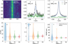 |
Fig. A.2 Simulation of the effect of varying background level on Plummer filament fitting. (a): The generated filament on top of the background. (b,c) The results of the fit for two different levels of background noise, with the original Plummer filament plotted with blue dashed lines, the background with green solid lines, and the sum of the Plummer and background with black lines. Frame b shows a stronger background w.r.t. the filament. (d,e,f) Violin plots of R (frame d). p (frame e), and FWHM (frame f) showing the results of the Plummer fit. Background noise decreases when moving right. The horizontal lines show the original Plummer parameters (dashed lines) and the median for our simulation (dotted line). |
To test how assuming a certain background model affects Plummer fits, both filaments were fit with a Plummer model which assumed a linear background. The first filament is thus correctly fitted with an appropriate background model. The second filament is incorrectly fitted with a linear background. We then compare the results of these fits, seeing how derived parameters differ.
Figure A.3 shows the inputs and results of this simulation. Frames b and e show both the background sky fluctuation (dotted lines), and the background component (dash-dotted lines) for each fit. Median derived N0 , Rflat , p, and FWHM are listed in Table A.2. The discrepancy between the two fits increases as the polynomial factor c increases. N0 is overestimated in most fits, possibly due to additional emission from the sky fluctuations. At m = 0.1, the derived values for both models are fairly similar. However, at m ≥ 1, Rflat is significantly overestimated in filaments with a polynomial background component. As the polynomial grows larger, the shape of the filament becomes dominated by this component. Generally, p has a wider range when fitting a linear profile, and is slightly underestimated. Meanwhile, if m ≥ 1, values of p are overestimated in the polynomial profile. FWHM is more consistent, but is slightly overestimated in the polynomial filament. In general, simulating a filament with a strong polynomial background creates another, more diffuse filamentary structure on top of the Plummer model, leading to increased width in fits.
A.2.3 Comparing fits to real data using a polynomial background model
We have tested a Plummer fit to our four fields, but assuming a polynomial background component. As priors in our fit, we use the derived parameters from Table D.1, and initially assume the polynomial term c = 0.0. Median profiles for q = 1–2 profiles are shown in Fig. A.4, and median values in Table A.3. (For linear fits, the profiles are shown in Fig. 4). The profile widths in G17 differ by up to 70% in q = 2 filament segments. This discrepancy is only about 20% in G202. The parameter p is lower in polynomial fits to G17, but significantly higher in G202.
Results of simulations comparing fits to a Plummer filament with a linear or polynomial background.
In contrast, OMC-3 can be fit equally well by a linear and polynomial background. Median values in G208 Nℱ are nearly the same in both fits. N0 in G208 Nℋ differs by no more than 4%. Rflat differs by 20% (0.01 pc) and p by less than 9%. The differences between the two fits are all within the 1-σ standard deviation. In fits using Spitzer extinction, as well as Herschel and ArTéMiS data of filament segments in OMC-3, Juvela & Mannfors (2023) also do not see notable difference in Rflat, p, or FWHM.
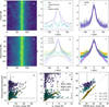 |
Fig. A.3 Results of simulations comparing filaments with a linear or polynomial background component. (Top row): A simulated filament with a linear background. (Middle row): A simulated filament with a polynomial background. Both filaments also have random sky fluctuations with powerlaw index k = -2. Frame a/d: The simulated filament, m = 1.0. Frame b/e: Components of the filament at different values of m: the sky (dotted line), initial Plummer (dashed line), the initial background component (dash-dotted lines), and the median profile (solid line). Yellow corresponds to the flattest background component (m = 0.1), turquoise to m = 1.0, and purple to the strongest background component (m = 2.0). Frame c/f: Individual profiles (solid lines) and Plummer fits (dashed lines) to selected profiles in each map. Colors correspond to different strengths as in the previous frames. (Bottom row): Rflat (g), p (h), and FWHM (i) calculated for the profiles with a linear background (x-axis) and a polynomial background (y-axis). Colors are as in frame e. The vertical and horizontal dashed lines mark the initial parameter value. |
A.3 Distance variation
We further studied the effect of distance on derived Plummer parameters using a simulated filament, once again with S/N = 100 and relatively weak background fluctuations, and FWHM = 20.78 pixels (corresponding to a pixel size of 4.8× 10⁻³ pc assuming a physical FWHM width of 0.1 pc). To simulate hierarchical structure within the ISM, we further added a wide Gaussian component with σ = 125 pixels (0.6 pc), half the original mapsize. This component is fainter and significantly wider than the main Plummer filament. We also added eight small spherical Gaussian clumps of width σ = 5–12 pixels to simulate smaller- scale hierarchical structure. The clumps are described by the formula exp  , where x and y are the coordinates of each pixel, x0 and y0 the central pixel coordinates of the clump, and σ the width of the Gaussian clump. The peak intensity of each clump is 1.0 before regridding.
Median Plummer parameters calculated assuming a linear or polynomial background.
The original filament was convolved to distances of 250 pc, 500 pc, 1 kpc, 2 kpc, and 4 kpc. The map was also reprojected to simulate increasing pixel size, thus, the size of the map in pixels also decreases with increased distance. The background sky, filament, noise, wide component, and clumps were generated at the beginning of the simulation and thus do not change during one run. The results of this simulation are shown in Fig. A.5. The first row shows the filament at different distances, the second row the profile (with all components) and fitted Plummer model, and the bottom violin plots of for the estimated R, p, and FWHM. Given an assumed intrinsic width of 0.1 pc, we estimate a relation between FWHM and distance of FWHM ≈ 1.7 × 10⁻⁴ ∙ d [pc] + 0.10, (Fit 1) a shallower relation that that derived in this paper. When we also allow the (fitted) intrinsic width to vary, this results in a fit of FWHM ≈ 1.1 × 10⁻⁴ ∙ d + 0.25 (Fit 2). This larger initial width is because of the blending of the large-scale Gaussian background structure with the Plummer filament.
We further perform this simulation with and without large- scale structures or small clumps, and by assuming S/N = 10 and S/N = 100, for a sample of 20 random realizations. We list the results of these tests in Table A.4. Varying the S/N between 10 and 100, but keeping the other parameters the same, changes the FWHM at 2 kpc by only (1.4±0.7)%. Whether Gaussian clumps are included or not changes FWHM at 2 kpc by (7.7±1.8)%, and in fact small-scale structures slightly compensate for the increase in FWHM due to distance. In contrast, the difference in FWHM at 2 kpc is around (42.8±2.8)% larger when large-scale background structures are included. However, even in tests without large-scale structure or clumps, FWHM can increase by up to 3×FW H MTrue at 2 kpc. In the final three columns of Table A.4 we list the slope, y-intercept value (i.e., the FWHM at d = 0 pc), and calculated FWHM at 2 kpc for Fit 2. Though the initial simulated Plummer filament has a width of 0.1 pc, in fits which include large-scale structures, the fitted intrinsic width is 0.2– 0.3 pc. In contrast, the four fits which do not include these large Gaussian structures have fitted intrinsic widths of 0.12–0.13 pc.
It is clear from these simulations that at least part of the distance relation could be due to the presence of hierarchical and large-scale structures. Furthermore, as real filaments such as those observed in the main paper are more complex than these ideal, straight filaments they may be further artificially widened. This is a likely explanation for the steeper relation found for our data, when compared with these simulations.
A.4 Range of offsets from the filament center
Previous studies have suggested that fitted parameters can change significantly depending on what range of offsets from the filament center Gaussian fitting is performed (Panopoulou et al. 2017). We tested this for Plummer fits using one of our fields, G208 Nℋ. The original data use 100 pixels on either side of the filament center, corresponding to ~1.16 pc in physical space (for a total map width of 2.5 pc). The map size is decreased to 75, 50, and 25 pixels per side (corresponding to ∼0.88, 0.59, and 0.30 pc, respectively). Plummer parameters are calculated with asymmetric fits, and the results are shown in Fig. A.6. We do not distinguish between filament quality flag in this test.
Unlike the study of Panopoulou et al. (2017), we do not find any difference in derived Plummer parameters with increased offset from filament center. Even when reducing the fitted area to ~0.12 pc, at which point the full filament width is not sampled, the derived FWHM stays remarkably consistent, though individual p and Rflat parameters begin to vary. In the case of a more complex, multiple-filament structure such as that in G202, a slight dependence between fitting area and FWHM is observed.
Derived distance-FWHM relation and FWHM at 2 kpc for the different simulations.
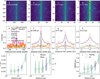 |
Fig. A.5 Simulated ideal filament observed at various distances. Top row: The simulated observation of the filament at the original resolution, and 500, 1000, and 2000 pc. Added Gaussian clumps are emphasized with black outlines. Middle row: Components of the observation at different distances. The background (orange solid lines), the original Plummer (blue dotted line), the wide Gaussian structure to simulate hierarchical structure (green dash-dotted lines), the mean small-scale Gaussian clump profile, and the resulting profile (pink solid lines). Frame e shows the original profile at the initial location of 125 pc, frames f-h the profiles from d = 500 pc to d = 2 kpc. The Plummer fit to the filament profile is shown with black dashed lines. Bottom row: Violin plots of derived Rflat (frame i), p (frame j), and FWHM (frame l). The mean and median values at each distance are plotted with gray lines. On frame l, we plot the intrinsic FWHM = 0.1 pc (teal solid line), as well as the fit where the FWHM of the fitted Plummer is fixed to 0.1 pc (blue dash-dotted line). |
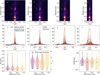 |
Fig. A.6 Simulation of the relation between fitted area from filament center and derived Plummer parameters. Top row (a–d) shows the data, with the original image in frame a. Middle row (e–h) show every profile in purple and the fitted Plummers in orange. The median profile is shown in black solid lines and the Plummer fit to the median Plummer in pale yellow dashed lines. The bottom row (i–k) show violin plots of filament width Rflat (frame i), slope p (frame j), and FWHM (frame k). The squares show the value for the parameter in the fit to the median profile (yellow line in the middle row). Sharp cut-offs at low values represent physical bounds set by the fitting, and are the same for all runs of this simulation. |
A.5 Comparison of 1D and 2D convolution
In this paper we have mainly used 1D convolution, in which each Plummer profile is convolved using a Gaussian. However, it is also possible to perform Plummer fitting by convolving the entire image with a 2D Gaussian. While there is no difference between a Gaussian convolved by Gaussian in one or two dimensions, the same is not necessarily true for a Plummer function. We thus performed tests of a simulated filament with S/N = 100 and convolution kernel σ = 3.0, and fit symmetric Plummer models with both a 1D and 2D convolution.
We performed this test with three filaments of varying background fluctuation, shown in Fig. A.7, frames d, h, and l. The median profiles for the original filament components are shown in the first column, the 1D fit in the second in purple, and the 2D fit in the third in gray. Derived Plummer parameters are listed in Table A.5. Violin plots of derived Rflat, p, and FWHM are shown in Fig. A.8.
As seen in the previous section, increasing filament strength results in decreased spread in Plummer parameters. The spread in 1D convolution is larger, as adjacent rows are not so well correlated. In fields with S/Nfilament >8, the median values are very similar. This is especially true for FWHM, in which the median values differ by under 10%. Due to its faster computing time (Fig. A.9), the 1D convolution is a viable choice.
Appendix B Additional tables
We present additional tables and data used in this paper. Fig. B.1 shows the three other ArTéMiS fields. Centers of the empty reference regions are listed in Table B.2, uncertainties on symmetric and asymmetric fits to an ideal filament in Tables B.3 and B.4, and median S/Nfilament of each field in Table B.5 for all quality flags. Finally, the results of wavelet analysis are shown in Table B.6.
Appendix C Testing the flux recovery of uvcombine
To test whether feathering recovered all flux, we performed simulations of an ideal filament with several Gaussian clumps. A Plummer filament and the clumps are shown in Fig. C.1a. The ideal map was convolved with a beam of 25′′ and white noise amounting to 1% of peak emission added to create the Herschel image (Fig. C.1b). The small-scale ArTéMiS image (Fig. C.1c) was created by subtracting an image convolved by 2′ from an image convolved by 8.5″, then adding white noise of 2% of peak emission.
The feathered result is shown in frame d, and the difference between the ideal and feathered images in frame e. The difference is under three percent of the original flux, showing that most signal is recovered by feathering. This effect worsens with decreasing S/N, but is not significant especially in q = 1–2 filaments.
Appendix D Plummer parameters
The following section presents derived Plummer parameters for the three regions studied in this paper. Tables D.1–D.2 list the median derived Plummer parameters for asymmetric and symmetric fits. Violin plots of the same results are shown in Fig. D.1 for asymmetric fits.
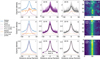 |
Fig. A.7 Plummer fits using 1D and 2D convolution to filaments of three different strengths. (First column) Components of the simulated filament. Median profile (solid blue line), original Plummer without noise (black dotted line) and with noise (solid pink line), the Plummer fit to only the Plummer with noise (dash-dotted line), the background sky (orange solid line), and the Plummer fit to the full simulated filament (blue dash-dotted line). (Second column) Individual profiles (solid lines) and 1-D Plummer fits (dashed lines) to each row of the profile. Median profile, and the median and mean Plummer fits are shown in black solid, dashed, and dash-dotted lines, respectively. (Third column) Same as the second column, but for the 2D Plummer fit. (Fourth column) The simulated filament. |
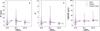 |
Fig. A.8 Comparison of parameters derived for Plummer fits to filaments using 1-D and 2-D convolution. The 1D Plummer fit is in purple and the 2D in gray. Mean of each set is shown with purple dashed lines, and median with black dash-dotted lines. The original Plummer parameter is shown with the black dotted line. |
Results of the simulations comparing 1 D and 2 D Plummer fitting to a simulated filament.
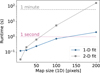 |
Fig. A.9 Time taken to run 1D (blue circles) and 2D (gray squares) Plummer analysis of maps of various sizes. These maps have a high S/N, comparable to the third row in Fig. A.7. |
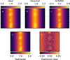 |
Fig. C.1 Test of data feathering. (a) Simulated filament and clumps. (b) Frame a convolved with a 25″ beam. (c) Frame a convolved to represent ArTéMiS observations. (d) Frames b and c feathered together with uvcombine. (e) Difference between the feathered and ideal images. |
References
- André, P., Men’shchikov, A., Bontemps, S., et al. 2010, A&A, 518, L102 [NASA ADS] [CrossRef] [EDP Sciences] [Google Scholar]
- André, P., Di Francesco, J., Ward-Thompson, D., et al. 2014, in Protostars and Planets VI, eds. H. Beuther, R. S. Klessen, C. P. Dullemond, & T. Henning, 27 [Google Scholar]
- André, P., Revéret, V., Könyves, V., et al. 2016, A&A, 592, A54 [NASA ADS] [CrossRef] [EDP Sciences] [Google Scholar]
- André, P. J., Palmeirim, P., & Arzoumanian, D. 2022, A&A, 667, L1 [CrossRef] [EDP Sciences] [Google Scholar]
- Aniano, G., Draine, B. T., Gordon, K. D., & Sandstrom, K. 2011, PASP, 123, 1218 [Google Scholar]
- Arzoumanian, D., André, P., Didelon, P., et al. 2011, A&A, 529, L6 [NASA ADS] [CrossRef] [EDP Sciences] [Google Scholar]
- Arzoumanian, D., André, P., Peretto, N., & Könyves, V. 2013, A&A, 553, A119 [NASA ADS] [CrossRef] [EDP Sciences] [Google Scholar]
- Arzoumanian, D., André, P., Könyves, V., et al. 2019, A&A, 621, A42 [NASA ADS] [CrossRef] [EDP Sciences] [Google Scholar]
- Astropy Collaboration (Robitaille, T. P., et al.) 2013, A&A, 558, A33 [NASA ADS] [CrossRef] [EDP Sciences] [Google Scholar]
- Bally, J., Langer, W. D., Stark, A. A., & Wilson, R. W. 1987, ApJ, 312, L45 [NASA ADS] [CrossRef] [Google Scholar]
- Beckwith, S. V. W., Sargent, A. I., Chini, R. S., & Guesten, R. 1990, AJ, 99, 924 [Google Scholar]
- Benedettini, M., Schisano, E., Pezzuto, S., et al. 2015, MNRAS, 453, 2036 [NASA ADS] [CrossRef] [Google Scholar]
- Berriman, G. B., Good, J. C., Laity, A. C., et al. 2004, in Astronomical Society of the Pacific Conference Series, 314, Astronomical Data Analysis Software and Systems (ADASS) XIII, eds. F. Ochsenbein, M. G. Allen, & D. Egret, 593 [NASA ADS] [Google Scholar]
- Carey, S. J., Clark, F. O., Egan, M. P., et al. 1998, ApJ, 508, 721 [Google Scholar]
- Chen, M. C.-Y., Di Francesco, J., Pineda, J. E., Offner, S. S. R., & Friesen, R. K. 2022, ApJ, 935, 57 [NASA ADS] [CrossRef] [Google Scholar]
- Chini, R., Reipurth, B., Ward-Thompson, D., et al. 1997, ApJ, 474, L135 [NASA ADS] [CrossRef] [Google Scholar]
- Clark, P. C., & Glover, S. C. O. 2014, MNRAS, 444, 2396 [CrossRef] [Google Scholar]
- Dewangan, L. K., Ojha, D. K., Sharma, S., et al. 2020, ApJ, 903, 13 [Google Scholar]
- Elmegreen, D. M., & Elmegreen, B. G. 1979, AJ, 84, 615 [Google Scholar]
- Evans, Neal J. I., Dunham, M. M., Jørgensen, J. K., et al. 2009, ApJS, 181, 321 [NASA ADS] [CrossRef] [Google Scholar]
- Federrath, C. 2016, MNRAS, 457, 375 [Google Scholar]
- Federrath, C., Rathborne, J. M., Longmore, S. N., et al. 2016, ApJ, 832, 143 [NASA ADS] [CrossRef] [Google Scholar]
- Fiege, J. D., & Pudritz, R. E. 2000, MNRAS, 311, 105 [NASA ADS] [CrossRef] [Google Scholar]
- Ge, Y., & Wang, K. 2022, ApJS, 259, 36 [NASA ADS] [CrossRef] [Google Scholar]
- Goldsmith, P. F. 2001, ApJ, 557, 736 [Google Scholar]
- Good, J., & Berriman, G. B. 2019, in Astronomical Society of the Pacific Conference Series, 523, Astronomical Data Analysis Software and Systems XXVII, eds. P. J. Teuben, M. W. Pound, B. A. Thomas, & E. M. Warner, 685 [NASA ADS] [Google Scholar]
- Goodman, A. A., Rosolowsky, E. W., Borkin, M. A., et al. 2009, Nature, 457, 63 [NASA ADS] [CrossRef] [Google Scholar]
- Griffin, M. J., Abergel, A., Abreu, A., et al. 2010, A&A, 518, L3 [EDP Sciences] [Google Scholar]
- Großschedl, J. E., Alves, J., Meingast, S., et al. 2018, A&A, 619, A106#17 [Google Scholar]
- Guo, W., Chen, X., Feng, J., et al. 2022, ApJ, 938, 44 [NASA ADS] [CrossRef] [Google Scholar]
- Güsten, R., Nyman, L. Å., Schilke, P., et al. 2006, A&A, 454, L13 [NASA ADS] [CrossRef] [EDP Sciences] [Google Scholar]
- Hacar, A., Tafalla, M., Forbrich, J., et al. 2018, A&A, 610, A77 [NASA ADS] [CrossRef] [EDP Sciences] [Google Scholar]
- Harris, C. R., Millman, K. J., van der Walt, S. J., et al. 2020, Nature, 585, 357 [NASA ADS] [CrossRef] [Google Scholar]
- Hartmann, L., & Burkert, A. 2007, ApJ, 654, 988 [NASA ADS] [CrossRef] [Google Scholar]
- Heitsch, F., & Hartmann, L. 2008, ApJ, 689, 290 [NASA ADS] [CrossRef] [Google Scholar]
- Hennebelle, P. 2013, A&A, 556, A153 [NASA ADS] [CrossRef] [EDP Sciences] [Google Scholar]
- Hennebelle, P., & André, P. 2013, A&A, 560, A68 [NASA ADS] [CrossRef] [EDP Sciences] [Google Scholar]
- Herschel Science Centre 2013, PACS Observers’ Manual, Tech. Rep. HERSCHEL-HSC-DOC-0832, ESA [Google Scholar]
- Hill, T., André, P., Arzoumanian, D., et al. 2012, A&A, 548, L6 [NASA ADS] [CrossRef] [EDP Sciences] [Google Scholar]
- Howard, A. D. P., Whitworth, A. P., Marsh, K. A., et al. 2019, MNRAS, 489, 962 [NASA ADS] [CrossRef] [Google Scholar]
- Hunter, J. D. 2007, Comput. Sci. Eng., 9, 90 [NASA ADS] [CrossRef] [Google Scholar]
- Juvela, M., & Mannfors, E. 2023, A&A, 671, A111 [NASA ADS] [CrossRef] [EDP Sciences] [Google Scholar]
- Juvela, M., Malinen, J., & Lunttila, T. 2012, A&A, 544, A141 [NASA ADS] [CrossRef] [EDP Sciences] [Google Scholar]
- Juvela, M., Demyk, K., Doi, Y., et al. 2015, A&A, 584, A94 [NASA ADS] [CrossRef] [EDP Sciences] [Google Scholar]
- Kainulainen, J., Federrath, C., & Henning, T. 2014, Science, 344, 183 [NASA ADS] [CrossRef] [Google Scholar]
- Kainulainen, J., Hacar, A., Alves, J., et al. 2016, A&A, 586, A27 [NASA ADS] [CrossRef] [EDP Sciences] [Google Scholar]
- Kirk, H., Klassen, M., Pudritz, R., & Pillsworth, S. 2015, ApJ, 802, 75 [NASA ADS] [CrossRef] [Google Scholar]
- Könyves, V., André, P., Men’shchikov, A., et al. 2015, A&A, 584, A91 [Google Scholar]
- Li, P. S., Lopez-Rodriguez, E., Soam, A., & Klein, R. I. 2022, MNRAS, 514, 3024 [NASA ADS] [CrossRef] [Google Scholar]
- Li, X.-M., Zhang, G.-Y., Men’shchikov, A., et al. 2023, A&A, 674, A225 [NASA ADS] [CrossRef] [EDP Sciences] [Google Scholar]
- Liu, T., Li, P. S., Juvela, M., et al. 2018, ApJ, 859, 151 [NASA ADS] [CrossRef] [Google Scholar]
- Malinen, J., Juvela, M., Collins, D. C., Lunttila, T., & Padoan, P. 2011, A&A, 530, A101 [NASA ADS] [CrossRef] [EDP Sciences] [Google Scholar]
- Malinen, J., Juvela, M., Rawlings, M. G., et al. 2012, A&A, 544, A50 [NASA ADS] [CrossRef] [EDP Sciences] [Google Scholar]
- Mattern, M., Kainulainen, J., Zhang, M., & Beuther, H. 2018, A&A, 616, A78 [NASA ADS] [CrossRef] [EDP Sciences] [Google Scholar]
- Megeath, S. T., Gutermuth, R., Muzerolle, J., et al. 2012, AJ, 144, 192 [NASA ADS] [CrossRef] [Google Scholar]
- Men’shchikov, A., André, P., Didelon, P., et al. 2010, A&A, 518, L103 [Google Scholar]
- Miettinen, O., Mattern, M., & André, P. 2022, A&A, 667, A90 [NASA ADS] [CrossRef] [EDP Sciences] [Google Scholar]
- Miville-Deschênes, M. A., Martin, P. G., Abergel, A., et al. 2010, A&A, 518, L104 [NASA ADS] [CrossRef] [EDP Sciences] [Google Scholar]
- Moeckel, N., & Burkert, A. 2015, ApJ, 807, 67 [NASA ADS] [CrossRef] [Google Scholar]
- Molinari, S., Swinyard, B., Bally, J., et al. 2010, A&A, 518, L100 [NASA ADS] [CrossRef] [EDP Sciences] [Google Scholar]
- Montillaud, J., Juvela, M., Vastel, C., et al. 2019a, A&A, 631, L1 [NASA ADS] [CrossRef] [EDP Sciences] [Google Scholar]
- Montillaud, J., Juvela, M., Vastel, C., et al. 2019b, A&A, 631, A3 [NASA ADS] [CrossRef] [EDP Sciences] [Google Scholar]
- Myers, P. C. 2009, ApJ, 700, 1609 [Google Scholar]
- Ormel, C. W., Min, M., Tielens, A. G. G. M., Dominik, C., & Paszun, D. 2011, A&A, 532, A43 [NASA ADS] [CrossRef] [EDP Sciences] [Google Scholar]
- Ostriker, J. 1964, ApJ, 140, 1056 [Google Scholar]
- Padoan, P., & Nordlund, Å. 2011, ApJ, 730, 40 [Google Scholar]
- Padoan, P., Juvela, M., Goodman, A. A., & Nordlund, Å. 2001, ApJ, 553, 227 [NASA ADS] [CrossRef] [Google Scholar]
- Padoan, P., Nordlund, Å., Kritsuk, A. G., Norman, M. L., & Li, P. S. 2007, ApJ, 661, 972 [NASA ADS] [CrossRef] [Google Scholar]
- Palau, A., Estalella, R., Girart, J. M., et al. 2014, ApJ, 785, 42 [Google Scholar]
- Palmeirim, P., André, P., Kirk, J. et al. 2013, A&A, 550, A38 [NASA ADS] [CrossRef] [EDP Sciences] [Google Scholar]
- Pan, S., Liu, H.-L., & Qin, S.-L. 2023, MNRAS, 519, 3851 [NASA ADS] [Google Scholar]
- Panopoulou, G. V., Psaradaki, I., Skalidis, R., Tassis, K., & Andrews, J. J. 2017, MNRAS, 466, 2529 [NASA ADS] [CrossRef] [Google Scholar]
- Panopoulou, G. V., Clark, S. E., Hacar, A., et al. 2022, A&A, 657, L13 [NASA ADS] [CrossRef] [EDP Sciences] [Google Scholar]
- Peretto, N., André, P., Könyves, V. et al. 2012, A&A, 541, A63 [NASA ADS] [CrossRef] [EDP Sciences] [Google Scholar]
- Peretto, N., Fuller, G. A., Duarte-Cabral, A., et al. 2013, A&A, 555, A112 [NASA ADS] [CrossRef] [EDP Sciences] [Google Scholar]
- Peretto, N., Rigby, A., André, P., et al. 2020, MNRAS, 496, 3482 [NASA ADS] [CrossRef] [Google Scholar]
- Pilbratt, G. L., Riedinger, J. R., Passvogel, T., et al. 2010, A&A, 518, L1 [NASA ADS] [CrossRef] [EDP Sciences] [Google Scholar]
- Planck Collaboration XXVIII. 2016, A&A, 594, A28 [NASA ADS] [CrossRef] [EDP Sciences] [Google Scholar]
- Poglitsch, A., Waelkens, C., Geis, N., et al. 2010, A&A, 518, L2 [NASA ADS] [CrossRef] [EDP Sciences] [Google Scholar]
- Priestley, F. D., & Whitworth, A. P. 2020, MNRAS, 499, 3728 [Google Scholar]
- Revéret, V., André, P., Le Pennec, J., et al. 2014, SPIE Conf. Ser., 9153, 915305 [Google Scholar]
- Rivera-Ingraham, A., Ristorcelli, I., Juvela, M., et al. 2016, A&A, 591, A90 [NASA ADS] [CrossRef] [EDP Sciences] [Google Scholar]
- Robitaille, T., & Bressert, E. 2012, APLpy: Astronomical Plotting Library in Python, Astrophysics Source Code Library, [record ascl:1208.017] [Google Scholar]
- Sadavoy, S. I., di Francesco, J., André, P., et al. 2012, A&A, 540, A10 [NASA ADS] [CrossRef] [EDP Sciences] [Google Scholar]
- Sadavoy, S. I., Stutz, A. M., Schnee, S., et al. 2016, A&A, 588, A30 [NASA ADS] [CrossRef] [EDP Sciences] [Google Scholar]
- Salji, C. J., Richer, J. S., Buckle, J. V., et al. 2015, MNRAS, 449, 1782 [NASA ADS] [CrossRef] [Google Scholar]
- Schisano, E., Rygl, K. L. J., Molinari, S., et al. 2014, ApJ, 791, 27 [Google Scholar]
- Schneider, S., & Elmegreen, B. G. 1979, ApJS, 41, 87 [Google Scholar]
- Schuller, F., André, P., Shimajiri, Y., et al. 2021, A&A, 651, A36 [NASA ADS] [CrossRef] [EDP Sciences] [Google Scholar]
- Shetty, R., Kauffmann, J., Schnee, S., & Goodman, A. A. 2009, ApJ, 696, 676 [NASA ADS] [CrossRef] [Google Scholar]
- Shimajiri, Y., André, P., Ntormousi, E., et al. 2019, A&A, 632, A83 [NASA ADS] [CrossRef] [EDP Sciences] [Google Scholar]
- Shimajiri, Y., André, P., Peretto, N., et al. 2023, A&A, 672, A133 [NASA ADS] [CrossRef] [EDP Sciences] [Google Scholar]
- Shirley, Y. L., Evans, Neal J. I., Rawlings, J. M. C., & Gregersen, E. M. 2000, ApJS, 131, 249 [NASA ADS] [CrossRef] [Google Scholar]
- Smith, R. J., Glover, S. C. O., & Klessen, R. S. 2014, MNRAS, 445, 2900 [Google Scholar]
- Smith, R. J., Glover, S. C. O., & Klessen, R. S., & Fuller, G. A. 2016, MNRAS, 455, 3640 [NASA ADS] [CrossRef] [Google Scholar]
- Soam, A., Liu, T., Andersson, B. G., et al. 2019, ApJ, 883, 95 [NASA ADS] [CrossRef] [Google Scholar]
- SPIRE Consortium, Valtchanov, I., & Herschel Science Centre 2011, SPIRE Observers’ Manual, Tech. Rep. HERSCHEL-DOC-0798, ESA [Google Scholar]
- Suri, S., Sánchez-Monge, Á., Schilke, P., et al. 2019, A&A, 623, A142 [NASA ADS] [CrossRef] [EDP Sciences] [Google Scholar]
- Takahashi, S., Ho, P. T. P., Teixeira, P. S., Zapata, L. A., & Su, Y.-N. 2013, ApJ, 763, 57 [Google Scholar]
- Tang, Y.-W., Koch, P. M., Peretto, N., et al. 2019, ApJ, 878, 10 [Google Scholar]
- Tokuda, K., Minami, T., Fukui, Y., et al. 2022, ApJ, 933, 20 [Google Scholar]
- Traficante, A., Fuller, G. A., Duarte-Cabral, A., et al. 2020, MNRAS, 491, 4310 [Google Scholar]
- Vázquez-Semadeni, E., Banerjee, R., Gómez, G. C., et al. 2011, MNRAS, 414, 2511 [CrossRef] [Google Scholar]
- Virtanen, P., Gommers, R., Oliphant, T. E., et al. 2020, Nat. Methods, 17, 261 [Google Scholar]
- Wang, K., Zhang, Q., Testi, L., et al. 2014, MNRAS, 439, 3275 [Google Scholar]
- Wang, K., Testi, L., Burkert, A., et al. 2016, ApJS, 226, 9 [NASA ADS] [CrossRef] [Google Scholar]
- Yamada, R. I., Fukui, Y., Sano, H., et al. 2022, MNRAS, 515, 1012 [NASA ADS] [Google Scholar]
- Zavagno, A., André, P., Schuller, F., et al. 2020, A&A, 638, A7 [NASA ADS] [CrossRef] [EDP Sciences] [Google Scholar]
- Zhang, G.-Y., André, P., Men’shchikov, A., & Wang, K. 2020, A&A, 642, A76 [NASA ADS] [CrossRef] [EDP Sciences] [Google Scholar]
- Zhang, C., Zhang, G.-Y., Li, J.-Z., & Li, X.-M. 2022, Res. Astron. Astrophys., 22, 055012 [CrossRef] [Google Scholar]
- Zheng, Y.-Q., Wang, H.-C., Ma, Y.-H., & Li, C. 2021, Res. Astron. Astrophys., 21, 188 [Google Scholar]
Atacama Large Millimeter Array.
http://www.apex-telescope.org/instruments/pi/artemis/; ARchitectures de bolomètres pour des TElescopes à grand champ de vue dans le domaine sub-MIllimétrique au Sol.
Based on observations with the APEX telescope under program ID 0101.F-9305(A). APEX is a collaboration between the Max-Planck- Institut fuer Radioastronomie, the European Southern Observatory, and the Onsala Observatory.
scipy.stats.skew (bias=True).
scipy.stats.kurtosis (fisher=True).
All Tables
Pearson correlation coefficients between column density, skewness, S, and kurtosis, K.
Skewness and kurtosis calculated for simulated filaments with the symmetric Plummer parameters of our q = 1 profiles.
Results of simulations comparing fits to a Plummer filament with a linear or polynomial background.
Median Plummer parameters calculated assuming a linear or polynomial background.
Derived distance-FWHM relation and FWHM at 2 kpc for the different simulations.
Results of the simulations comparing 1 D and 2 D Plummer fitting to a simulated filament.
All Figures
|
Fig. 1 G208 with Herschel and ArTéMiS. (a) Herschel 350 μm surface brightness map (Iℋ(350), resolution ≈ 20″); (b) ArTéMiS 350 μm surface brightness map; (c) The combined map obtained by feathering (Iℱ(350)). The beam is shown in the lower left corner of each image. The resolution of images (b) and (c) is around 10″. |
| In the text | |
|
Fig. 2 Extracted filaments on the Herschel column density maps. Top row: Column density images (FWHM = 20″) of fields G17, G202, and G208 showing the extracted filaments in each field. Filament quality is marked by color of symbols: q = 1 (yellow circles), q = 2 (purple circles), q = 3 (orange crosses), and q = 4 (green crosses). The yellow contour shows the limit of AV = 3 mag. Bottom row: Extracted filament profiles, in which the filament center is at the center of the image. |
| In the text | |
|
Fig. 3 Skewness (green dashed line) and kurtosis (gray dash-dotted line) along the filament spine of G17, G202, and G208 Nℋ and Nℱ. The right-hand y-axis shows column density along the filament spine (purple solid line). The faint gray horizontal line marks K = S = 0. S which falls outside of the green highlighted region is significant (see Sect. 4.2.1). |
| In the text | |
|
Fig. 4 Filament profiles in G17 (a), G202 (b), G208 Nℋ (c), and G208 Nℱ (d). The median filament profile is shown with solid lines, for quality 1 filaments (blue) and quality 1 and 2 (purple) profiles. The dash-dotted line shows the Plummer fit to the median filament profile. The dotted line shows the median Plummer profile, by taking the median of each individual Plummer parameter calculated. |
| In the text | |
|
Fig. 5 Observed dependence of FWHM on filament distance and observational resolution. Left: FWHM from asymmetric fits plotted against the distance of the field of each q = 1–2 profile (squares and crosses, respectively). For readability, the distance values include small added jitter. Median of each distribution is plotted with a solid line (q = 1) and dashed line (q = 2). Grey lines show the proposed relation of FWHM = 4 × HPBW (Panopoulou et al. 2022), as well as the Herschel (solid line) and ArTéMiS (dashed line) beamsizes. Right: Median value of each q = 1–2 dataset as a function of observational resolution in pc (solid squares). The errorbars represent the standard deviation of the FWHM widths in each dataset. Grey lines show relations of FWHM = [1,2,4] × HPBW. In both frames, we also include values from the literature (see text for references): Herschel continuum (yellow triangles), other continuum (orange diamonds), mean deconvolved filament widths from Fig. 1 of Panopoulou et al. (2022) (yellow circles), and values from Juvela & Mannfors (2023) with solid plusses (LR and HR in yellow, AR with orange, and MIR with red). The errorbars represent either the published uncertainty or a 30% uncertainty on the FWHM. In the left frame only, we show additional literature values from CO (purple stars) and NH3 (purple hexagon) observations. Solid symbols represents deconvolved widths, those without beam deconvolution are shown with outlines. |
| In the text | |
|
Fig. 6 Plummer FWHM plotted against the column density at the filament spine for Herschel fields G17 (a), G202 (b), and G208 (c), and the Nℱ map (d), for filaments of quality 1 (purple circles) and 2 (black crosses). Transparent symbols show profiles for which p > 10. |
| In the text | |
|
Fig. 7 Comparison of G208 Nℱ and Nℋ,crop filament shapes. Frame a: Profiles of Nℋ (orange) and Nℱ (purple) q = 1–2 filaments. Median profiles are plotted with solid and dashed lines for q = 1 and q = 2 profiles, respectively. Frames b-d: histograms of p (b), Rflat (d), and FWHM (c) for all q = 1–2 filaments in field G208. Medians and means for each distributions are plotted in dashed and dotted lines, respectively. The shaded areas correspond to the central 1-σ regions of the distributions. |
| In the text | |
|
Fig. 8 Comparison of derived N(H2) in G208. N(H2) along the filament crest for the Nℱ (purple dashed line) and Nℋ,crop (orange solid line). The Nℋ,crop map is at 20″ resolution, and Nℱ has been convolved to the same 20′′ resolution. |
| In the text | |
|
Fig. 9 Clump ellipses (cyan) plotted on top of the Nℋ,crop (left) and Nℱ (right) column density maps. The three clumps removed from analysis are drawn with white outlines on the Nℱ map. The orange circle shows the region used for determining the RMS noise. |
| In the text | |
|
Fig. 10 Comparison of clump properties found in Nℋ,crop (gray) and Nℱ (purple dotted) column density maps. The corresponding median values are plotted with gray dashed and purple dash-dotted lines for Nℋ,crop and Nℱ, respectively. |
| In the text | |
|
Fig. 11 SEDs of the four brightest clumps in each field, at 160–500 µm. The dashed lines represent MBB fits with constant β =1.8 for each clump. The best-fit temperature for each clump is listed in the legend. |
| In the text | |
|
Fig. 12 Comparison between column densities derived in this work (NM) and in Schuller et al. (2021) (NS) using a combinations of Herschel and ArTéMiS observations. Frame a: This work. Frame b: Schuller et al. (2021), APEX project 098.F-9304. Frame c: Difference between this work and that of Schuller. The contours correspond to NM = (0, 0.25, 0.5, 1.0) × 1023 cm−2 Frame d: Comparison plot between N(H2) values. The black dashed line represents a 1–1 relation, while the colored lines give the linear fits between NM and NS, with colors corresponding to the contours in frame c. |
| In the text | |
|
Fig. 13 Comparison of symmetric and asymmetric Plummer fits for all fields. Rflat (top row), p (middle), and FWHM (bottom row) for symmetric (x-axes) and asymmetric (y-axes) fits. The q = 1 profiles are plotted with yellow circles and q = 2 profiles with green triangles. The gray solid line shows a 1:1 relation and the gray dashed lines highlight the allowed upper and lower limits of the Plummer parameters. |
| In the text | |
|
Fig. 14 Profiles of the q = 1 filament with the largest offset in each of the four fields. The pink solid line corresponds to the observed profile, the blue dotted line to the symmetric Plummer fit and the black dashed line to the asymmetric Plummer fit. |
| In the text | |
|
Fig. 15 Fit to the median profile plotted against (y-axis) the median values calculated separately for each filament profile (x-axis). The gray solid line represents a relation of y = x. Quality flags are represented by a star, square, circle, and triangle, in order of decreasing quality. The fit to the entire field, regardless of quality flag, is shown by an asterisk. The dashed lines represent upper and lower bounds to the fits. In frame 1, the color of the line corresponds to the field. |
| In the text | |
|
Fig. 16 FWHM values for all four datasets, calculated using the Plummer formula (Eq. (4)) with no term for offset (x-axis) and including ∆r (y-axis). The gray line plots a 1:1 relation. |
| In the text | |
|
Fig. A.1 Effect of varying S/N on Plummer filament fitting. (a) Profile showing the original Plummer without noise (black plusses), the fit with S/N = 2 (black solid line), S/N = 5 (teal dotted line), and S/N = 10 (dash- dotted line). The simulated filament profile assuming S/N = 2 is plotted with faint gray. (b–d) violin plots of derived FWHM, R, and p with increasing S/N. The dotted line corresponds to the original Plummer parameter, R = 6.0 and p = 2.0. |
| In the text | |
|
Fig. A.2 Simulation of the effect of varying background level on Plummer filament fitting. (a): The generated filament on top of the background. (b,c) The results of the fit for two different levels of background noise, with the original Plummer filament plotted with blue dashed lines, the background with green solid lines, and the sum of the Plummer and background with black lines. Frame b shows a stronger background w.r.t. the filament. (d,e,f) Violin plots of R (frame d). p (frame e), and FWHM (frame f) showing the results of the Plummer fit. Background noise decreases when moving right. The horizontal lines show the original Plummer parameters (dashed lines) and the median for our simulation (dotted line). |
| In the text | |
|
Fig. A.3 Results of simulations comparing filaments with a linear or polynomial background component. (Top row): A simulated filament with a linear background. (Middle row): A simulated filament with a polynomial background. Both filaments also have random sky fluctuations with powerlaw index k = -2. Frame a/d: The simulated filament, m = 1.0. Frame b/e: Components of the filament at different values of m: the sky (dotted line), initial Plummer (dashed line), the initial background component (dash-dotted lines), and the median profile (solid line). Yellow corresponds to the flattest background component (m = 0.1), turquoise to m = 1.0, and purple to the strongest background component (m = 2.0). Frame c/f: Individual profiles (solid lines) and Plummer fits (dashed lines) to selected profiles in each map. Colors correspond to different strengths as in the previous frames. (Bottom row): Rflat (g), p (h), and FWHM (i) calculated for the profiles with a linear background (x-axis) and a polynomial background (y-axis). Colors are as in frame e. The vertical and horizontal dashed lines mark the initial parameter value. |
| In the text | |
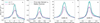 |
Fig. A.4 Same as Fig. 4, but for fits using a polynomial background. |
| In the text | |
|
Fig. A.5 Simulated ideal filament observed at various distances. Top row: The simulated observation of the filament at the original resolution, and 500, 1000, and 2000 pc. Added Gaussian clumps are emphasized with black outlines. Middle row: Components of the observation at different distances. The background (orange solid lines), the original Plummer (blue dotted line), the wide Gaussian structure to simulate hierarchical structure (green dash-dotted lines), the mean small-scale Gaussian clump profile, and the resulting profile (pink solid lines). Frame e shows the original profile at the initial location of 125 pc, frames f-h the profiles from d = 500 pc to d = 2 kpc. The Plummer fit to the filament profile is shown with black dashed lines. Bottom row: Violin plots of derived Rflat (frame i), p (frame j), and FWHM (frame l). The mean and median values at each distance are plotted with gray lines. On frame l, we plot the intrinsic FWHM = 0.1 pc (teal solid line), as well as the fit where the FWHM of the fitted Plummer is fixed to 0.1 pc (blue dash-dotted line). |
| In the text | |
|
Fig. A.6 Simulation of the relation between fitted area from filament center and derived Plummer parameters. Top row (a–d) shows the data, with the original image in frame a. Middle row (e–h) show every profile in purple and the fitted Plummers in orange. The median profile is shown in black solid lines and the Plummer fit to the median Plummer in pale yellow dashed lines. The bottom row (i–k) show violin plots of filament width Rflat (frame i), slope p (frame j), and FWHM (frame k). The squares show the value for the parameter in the fit to the median profile (yellow line in the middle row). Sharp cut-offs at low values represent physical bounds set by the fitting, and are the same for all runs of this simulation. |
| In the text | |
|
Fig. A.7 Plummer fits using 1D and 2D convolution to filaments of three different strengths. (First column) Components of the simulated filament. Median profile (solid blue line), original Plummer without noise (black dotted line) and with noise (solid pink line), the Plummer fit to only the Plummer with noise (dash-dotted line), the background sky (orange solid line), and the Plummer fit to the full simulated filament (blue dash-dotted line). (Second column) Individual profiles (solid lines) and 1-D Plummer fits (dashed lines) to each row of the profile. Median profile, and the median and mean Plummer fits are shown in black solid, dashed, and dash-dotted lines, respectively. (Third column) Same as the second column, but for the 2D Plummer fit. (Fourth column) The simulated filament. |
| In the text | |
|
Fig. A.8 Comparison of parameters derived for Plummer fits to filaments using 1-D and 2-D convolution. The 1D Plummer fit is in purple and the 2D in gray. Mean of each set is shown with purple dashed lines, and median with black dash-dotted lines. The original Plummer parameter is shown with the black dotted line. |
| In the text | |
|
Fig. A.9 Time taken to run 1D (blue circles) and 2D (gray squares) Plummer analysis of maps of various sizes. These maps have a high S/N, comparable to the third row in Fig. A.7. |
| In the text | |
|
Fig. C.1 Test of data feathering. (a) Simulated filament and clumps. (b) Frame a convolved with a 25″ beam. (c) Frame a convolved to represent ArTéMiS observations. (d) Frames b and c feathered together with uvcombine. (e) Difference between the feathered and ideal images. |
| In the text | |
Current usage metrics show cumulative count of Article Views (full-text article views including HTML views, PDF and ePub downloads, according to the available data) and Abstracts Views on Vision4Press platform.
Data correspond to usage on the plateform after 2015. The current usage metrics is available 48-96 hours after online publication and is updated daily on week days.
Initial download of the metrics may take a while.