| Issue |
A&A
Volume 689, September 2024
|
|
|---|---|---|
| Article Number | A329 | |
| Number of page(s) | 28 | |
| Section | The Sun and the Heliosphere | |
| DOI | https://doi.org/10.1051/0004-6361/202450069 | |
| Published online | 24 September 2024 | |
A solar rotation signature in cosmic dust: Frequency analysis of dust particle impacts on the Wind spacecraft
1
ETH Zürich, Institute for Particle and Astroparticle Physics, 8093 Zürich, Switzerland
2
ETH Zürich, Department of Environmental Systems Science, 8092 Zürich, Switzerland
3
Swiss Federal Research Institute WSL, 8903 Birmensdorf, Switzerland
4
Technische Universität Braunschweig, Institute of Geophysics and Extraterrestrial Physics, 38106 Braunschweig, Germany
5
Max Planck Institute for Solar System Research, 37077 Göttingen, Germany
6
University of Colorado, Boulder, Astrophysical and Planetary Sciences Department, Boulder, CO 80309, USA
7
University of Colorado, Boulder, Laboratory for Atmospheric and Space Physics, Boulder, CO 80309, USA
8
NASA Goddard Space Flight Center, Greenbelt, MD 20771, USA
9
University of Colorado, Boulder, Department of Physics, Boulder, CO 80309, USA
Received:
22
March
2024
Accepted:
6
July
2024
Abstract
Aims. Dust particle impacts on the Wind spacecraft were detected with its plasma wave instrument Wind/WAVES. Frequency analysis on the resulting dust impact time series has revealed spectral peaks indicative of a solar rotation signature. We investigated whether this solar rotation signature is embedded in the interplanetary or in the interstellar dust (ISD) and whether it is caused by co-rotating interaction regions (CIRs), by the sector structure of the interplanetary magnetic field (IMF), or by external effects.
Methods. We performed frequency analysis on different subsets of the data to investigate the origin of these spectral peaks, comparing segments of Wind’s orbit when the spacecraft moved against or with the ISD inflow direction and comparing the time periods of the ISD focusing phase and the ISD defocusing phase of the solar magnetic cycle. A superposed epoch analysis of the number of dust impacts during CIRs was used to investigate the systematic effect of CIRs. Case studies of time periods with frequent or infrequent occurrences of CIRs were performed and compared to synthetic data of cosmic dust impacts affected by CIRs. We performed similar case studies for time periods with a stable or chaotic IMF sector structure. The superposed epoch analysis was repeated for a time series of the spacecraft floating potential.
Results. Spectral peaks were found at the solar rotation period of ∼27 d and its harmonics at 13.5 d and 9 d. This solar rotation signature may affect both interplanetary and interstellar dust. The appearance of this signature correlates with the occurrence of CIRs but not with the stability of the IMF sector structure. The CIRs cause, on average, a reduction in the number of dust impact detections. Periodic changes of the spacecraft’s floating potential were found to partially counteract this reduction by enhancing the instrument’s sensitivity to dust impacts; these changes of the floating potential are thus unlikely to be the cause of the solar rotation signature.
Key words: Sun: heliosphere / Sun: magnetic fields / Sun: rotation / solar wind / zodiacal dust / dust / extinction
Corresponding author; This email address is being protected from spambots. You need JavaScript enabled to view it. .
© The Authors 2024
 Open Access article, published by EDP Sciences, under the terms of the Creative Commons Attribution License (https://creativecommons.org/licenses/by/4.0), which permits unrestricted use, distribution, and reproduction in any medium, provided the original work is properly cited.
This article is published in open access under the Subscribe to Open model. This email address is being protected from spambots. You need JavaScript enabled to view it. to support open access publication.
1. Introduction
Cosmic dust is highly prevalent in the Solar System (e.g. Brownlee 1985). Depending on its origin, one distinguishes between interplanetary dust particles (IDPs; e.g. Grün et al. 2001) and interstellar dust (ISD; e.g. Grün et al. 1993; Sterken et al. 2019). As the name suggests, IDPs originate in the Solar System. They are, for example, evaporated from comets, created through collisions of asteroids, or ejected from active moons. In contrast, ISD enters the heliosphere from the local interstellar medium. As such, ISD grains have hyperbolic orbits and are generally faster than the local escape speed (Grün et al. 1994), whereas IDPs are typically bound to elliptic orbits around the Sun (although IDPs can also reach sufficient speeds to escape the Solar System as β-meteoroids; e.g. Zook & Berg 1975; Wehry & Mann 1999; Czechowski & Mann 2010). Because the polarity of the interplanetary magnetic field (IMF) changes periodically with the 22 yr solar magnetic cycle, ISD is alternately focused towards or defocused away from the ecliptic plane with a 22 yr-periodicity (Gustafson & Misconi 1979; Sterken et al. 2012).
In situ, both IDPs and ISD are often jointly measured with dedicated dust detectors. The discovery of ISD in the Solar System, for example, was made with the dedicated dust detector onboard Ulysses (Grün et al. 1993). However, dust impacts on spacecraft can also be registered with instruments not intended for this purpose, such as plasma wave instruments.
Measurements of dust impacts with plasma wave antennas have been made, for example but not limited to, at Saturn on board Voyager 2 (Aubier et al. 1983; Gurnett et al. 1983) and Cassini (e.g. Kurth et al. 2006), during cometary approaches by the International Cometary Explorer (Gurnett et al. 1986) and by Deep Space 1 (Tsurutani et al. 2004), as well as at Mars on board Mars Atmosphere and Volatile Evolution (Andersson et al. 2015), at Earth by Cluster II (Vaverka et al. 2017) and the Magnetospheric Multiscale missions (Vaverka et al. 2018), by both spacecraft of the Solar Terrestrial Relations Observatory (STEREO; e.g. Meyer-Vernet et al. 2009, and references thereof), and in close vicinity to the Sun by Parker Solar Probe (Page et al. 2020) and Solar Orbiter (Zaslavsky et al. 2021).
Of particular interest for dust detections with plasma wave instruments is the Wind spacecraft (see Wilson et al. 2021 for a comprehensive review). The Wind mission was launched in 1994 to investigate the solar wind and its plasma processes in near-Earth space. In its almost 30 years of service, Wind’s electric field instrument, Wind/WAVES (Bougeret et al. 1995), has indirectly measured impacts of cosmic dust on the spacecraft. This was first reported by Malaspina et al. (2014), who found that the daily number of dust impacts is correlated with Wind’s orbital direction of motion around the Sun: More dust impacts were measured when the spacecraft moved against the preferential inflow direction of ISD than when it moved with the ISD inflow direction.
Some signals recorded by the two STEREO spacecraft were identified as impacts of nanometre-sized dust particles (“nanodust”; Zaslavsky et al. 2012); however, this was later contested (e.g. Kellogg et al. 2018). Kellogg et al. (2016) analysed the waveforms of the dust impacts on Wind in detail and concluded that the instrument is not sensitive to impacts of nanodust. They also found that the ISD impacts measured by Wind and STEREO were consistent when Wind and STEREO A/B were close to each other. A database of dust impacts on Wind was published by Malaspina & Wilson (2016) and is updated every few years.
This publication reports on the discovery of solar rotation signatures in dust impact data measured by plasma wave antennas (Sect. 4.1). The discovery of these signatures leads to the following investigations:
-
In Sect. 4.2 we discuss whether the solar rotation signatures stem from the interstellar or the interplanetary dust population, or from both.
-
In Sect. 4.3 we investigate whether the solar rotation signatures are imprinted on the dust detections by co-rotating interaction regions (CIRs).
-
In Sect. 4.4 we discuss whether the solar rotation signatures are imprinted on the dust detections by the IMF sector structure or crossings of the heliospheric current sheet.
-
In Sect. 4.5 we consider whether the solar rotation signatures are not dust signatures at all but caused by external effects.
One physical mechanism that may cause the solar rotation signatures is a local reduction or enhancement of dust particles whenever a CIR passes by the spacecraft. A similar dust depletion mechanism has been proposed in the past to occur close to the Sun during coronal mass ejections (CMEs; Ragot & Kahler 2003); this has been indirectly observed by Stenborg et al. (2023) using Parker Solar Probe. Numerical simulations have found that this effect can cause either a reduction or an enhancement of the local dust density at 1 AU (Wagner & Wimmer-Schweingruber 2009; O’Brien et al. 2018); a depletion of observed dust impacts on Wind coinciding with CMEs was discovered by St. Cyr et al. (2017). A superposed epoch analysis of dust impacts measured by Wind during CIRs is performed in Sect. 4.3.1 to investigate the effect of CIRs on the local dust environment measured by Wind.
Another possible mechanism that may cause the solar rotation signatures could be a periodic deflection of dust particles by the alternating IMF sector structure, which has been proposed as the origin of Jovian dust streams by Hamilton & Burns (1993). Hsu et al. (2010) and Flandes et al. (2011) report that both the IMF sector structure and CIRs act on Saturnian and Jovian dust streams, causing strong enhancements of nanodust particle measurements with the dust detectors on board Cassini and Ulysses, respectively. However, the particles of Jovian and Saturnian dust streams are assumed to have radii of roughly ∼10 nm (Zook et al. 1996; Hsu et al. 2011), which is smaller than the approximately submicron-sized range to which Wind is assumed to be sensitive (Malaspina et al. 2014). Spectral signatures of the solar rotation have also been found in the dust impact data measured by the STEREO spacecraft (Chadda et al., in prep.).
2. Dynamics of cosmic dust in the Solar System
Cosmic dust in the Solar System is primarily affected by three forces: solar gravity, solar radiation pressure (SRP), and the Lorentz force (Sect. 2.1). Of these forces, only the Lorentz force, through variations in the IMF, changes on timescales that can cause the solar rotation signatures. Therefore, the most salient properties of the IMF are presented in Sect. 2.2, including periodic changes induced by the IMF sector structure (Sect. 2.3) and by CIRs (Sect. 2.4).
2.1. Primary forces acting on cosmic dust in the Solar System
In heliocentric coordinates, both solar gravity and SRP are radially directed and thus are often combined into one term:
 (1)
(1)
where G is the gravitational constant, M⊙ the solar mass, md the mass of the dust particle, r the heliocentric distance,  the unit vector radially pointing away from the Sun, and β ≡ |FSRP|/|FG| is the ratio of SRP to solar gravity. The β-ratio is, for a given dust particle, a constant that depends on properties of the particle such as its composition, mass, and morphology (Sterken et al. 2019). For a given species of dust particles, the β-ratio is often given as a function of the particle mass or size (e.g. Gustafson 1994, Fig. 3; see also Fig. 1). The solar irradiance, and through it the SRP, only changes by about 0.1% over the solar 11 yr-cycle (Fröhlich & Lean 1998); this variance is disregarded in this study. Similarly, Poynting-Robertson drag is only relevant for long-term dynamics of IDPs and is, thus, not considered (Robertson 1937; Altobelli 2004).
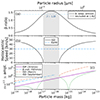 |
Fig. 1. Relevant dust properties versus particle mass. Top panel: β-ratio versus particle mass following the astronomical silicates of Gustafson (1994) adapted to have a maximum of β = 1.6 (Sterken et al. 2013). Middle panel: Subsequent heliocentric speed of ISD particles (solid black curve) dependent on the particle mass using Eq. (4); Earth’s orbital speed (dashed blue line) for comparison. Bottom panel: Signal amplitude of a single dust particle, taken as m v3.5 as per Eq. (3), for an IDP with an impact speed of 20 km/s (solid magenta line), a β-meteoroid of 50 km/s (dash-dotted blue line), and an ISD particle in March (dashed red curve) and in September (dotted green curve). No line was plotted for β-meteoroids above m > 10−16 kg because β-meteoroids are constrained to lower masses (Wehry & Mann 1999; Moorhead 2021). The secondary horizontal axis of the top panel gives the particle radius, assuming spherical and compact particles with a density of 2500 kg/m3 (Sterken et al. 2013). ISD with β > 1.38 (dashed blue horizontal in the top panel) cannot reach Earth’s orbit; it is excluded (grey-shaded area). |
The third relevant force acting on dust particles is the Lorentz force, which in terms of its acceleration is given by
 (2)
(2)
where qd/md is the dust particle’s charge-to-mass ratio, vd is the velocity of the dust particle, vsw is the velocity of the expanding solar wind, and Bsw is the magnetic field vector of the IMF.
Of these three forces, only the Lorentz force can cause short-term modulations of the dust environment that can lead to the observed solar rotation signatures (Sect. 4.1). Assuming that the mass of a dust particle is constant, these variations in the Lorentz force must be caused by a change of the dust particle’s surface charge, the solar wind speed, or the IMF.
The surface charge, qd, of a submicrometer dust particle in the IMF corresponds to a constant surface potential of roughly +5 V (Mukai 1981), and is higher for nanodust particles due to the “small particle effect” (Watson 1973). Although nanodust has charging timescales of multiple days (Ma et al. 2013), for submicrometer dust particles the charge can vary at 1 AU on a timescale of minutes (Sterken et al. 2022). The major contributions to the charging environment in the inner Solar System are solar UV radiation, which is assumed to be reasonably constant, and the solar wind. Therefore, knowing the spatial and time evolution of the solar wind and, especially, the IMF is essential for understanding the dynamics of cosmic dust in the heliosphere.
2.2. The large-scale interplanetary magnetic field
The large-scale IMF is typically described by an archimedean spiral; the magnetic field lines are “frozen” into the radially expanding solar wind and are wound up through the Sun’s rotation (Parker 1958). This “Parker spiral” has no polar component; its radial component is dominant close to the Sun, and its azimuthal component is dominant at larger heliocentric distances: at 1 AU the angle between the IMF and the radial direction is about 45°, whereas close to Jupiter this angle has increased to roughly 80° (Owens & Forsyth 2013). Close to the solar equatorial plane, the Parker spiral lies almost parallel to the equatorial plane. At higher latitudes, however, its radial component is significantly tilted with respect to the equatorial plane; the IMF gains a component along the z-axis of the solar ecliptic coordinate system1. At large heliocentric distances, where the azimuthal component is dominant over the radial, this z-component is negligible.
In simplified terms, the solar magnetic field can be described by a magnetic dipole that is at solar minimum roughly aligned with the solar rotation axis; thus, the field lines of the IMF point towards the Sun in one solar hemisphere and away from it in the other. Accordingly, a large component of the IMF points into the azimuthal direction in one hemisphere and into the anti-azimuthal direction in the other. Charged particles moving parallel to the ecliptic plane, such as ISD, thus experience a Lorentz force that in both hemispheres points either towards the ecliptic plane or away from it, depending on which polarity lies in which hemisphere. Thus, ISD particles are either focused towards or defocused away from the ecliptic plane (Morfill & Grün 1979; Landgraf 2000; Sterken et al. 2012).
The polarity of the IMF flips with the solar 11 yr cycle, causing alternating focusing phases and defocusing phases of ISD within the solar magnetic 22 yr-cycle (Sterken et al. 2012). Other periodic changes of the IMF correspond to its sector structure (Sect. 2.3) and to CIRs (Sect. 2.4), both of which are associated with the solar rotation period, which is ∼27 d for an observer on or at Earth.
2.3. The heliospheric current sheet and interplanetary magnetic field sector structure
The interface between the regions of opposite IMF polarities is referred to as the “heliospheric current sheet” (HCS). If the solar magnetic field were perfectly described by a dipole that is aligned with the solar rotation axis, the HCS would be a flat plane identical to the solar equatorial plane. However, even at solar minimum when the solar magnetic field is well-approximated by a dipole, the dipole axis and the rotation axis are slightly tilted with respect to each other. This warps the HCS into what is commonly called the “ballerina skirt” (e.g. Jokipii & Thomas 1981). Within the ecliptic plane, this ballerina skirt is apparent as sectors of opposing magnetic polarity; the HCS constitutes the sector boundaries. This “sector structure” co-rotates with the Sun (e.g. Owens & Forsyth 2013).
When the solar magnetic field is approximated reasonably well by a magnetic dipole close to solar minimum, the IMF features a two-sector structure. As the solar cycle progresses and higher multipole moments of the magnetic field increase in strength, the IMF often changes from a two-sector structure to a four-sector structure. These four sectors are generally not identically sized (e.g. Richardson 2018). Due to further warping of the HCS, an orbiting object such as Earth or Wind can experience more than four sector boundary crossings or even skim the HCS for an extended period of time (Owens & Forsyth 2013).
The IMF sector structure is known to imprint the solar rotation period on some cosmic dust particles like Jovian and Saturnian dust streams: because the IMF features opposite polarities on each side of the HCS, the Lorentz force points towards the ecliptic plane on one side of the sector boundary and away from it on the other, affecting charged particles such as ISD and IDPs. This was observed by Ulysses for Jovian dust streams: in one sector of the IMF a collimated stream of dust particles would move northward through the ecliptic plane, and in the other sector it would move southward through the ecliptic plane; thus, a spacecraft residing in the ecliptic plane would encounter streams of particles twice per solar rotation period. At higher latitudes, the spacecraft would only encounter the northernmost or southernmost point of inflection of the particle stream, which would occur only once per solar rotation (Hamilton & Burns 1993).
The timing of the Jovian dust streams observed by Ulysses was furthermore associated with CIRs (see Sect. 2.4) by Flandes et al. (2011); Table 1 of that reference indicates that successive Jovian dust streams may be separated by roughly half a solar rotation period at low jovigraphic latitudes and by a full solar rotation period at higher jovigraphic latitudes, which agrees with the scenario proposed by Hamilton & Burns (1993).
Continuously updated lists of sector boundary crossings of Earth and of the IMF sector structure are provided by Svalgaard (2023a,b). These lists are used to investigate whether the solar rotation signatures are caused by the IMF sector structure in Sect. 4.4.
2.4. Co-rotating interaction regions
How tightly the IMF is coiled around the Sun depends on the speed of the solar wind, vsw. Close to the ecliptic plane, the slow solar wind is emitted from the Sun’s streamer belt with vsw ≈ 400 km/s at 1 AU, resulting in an angle between the IMF and the radial direction of about 45° at 1 AU. A fast solar wind is emitted from coronal holes, reaching speeds of vsw ≈ 750 km/s and angles of about 30° at 1 AU between the IMF and the radial direction; the Parker spiral is wound less tightly for the fast solar wind compared to the slow solar wind. Thus, the slow and the fast solar wind must interface, generating “stream interaction regions” (SIRs). If SIRs persists for multiple solar rotations, they are referred to as “co-rotating interaction regions” (Richardson 2018).
The SIRs consist of compression regions, where the magnetic field strength and plasma density are increased, followed by rarefaction regions, where the magnetic field strength and plasma density relax to their unperturbed values (Richardson 2018). Therefore, inside a SIR the Lorentz force is enhanced, accelerating dust particles far more than the unperturbed slow solar wind does. This has been reported by Hsu et al. (2010) for Saturnian dust stream particles. As mentioned before, the Jovian dust streams have also been associated with CIRs by Flandes et al. (2011).
Jian et al. (2006) measured 365 encounters of Wind with SIRs from 1995 until 2004, about half of which persisted for multiple months (CIRs). This list was updated until 2009 by Jian (2021). Hajra & Sunny (2022) measured 290 CIRs encountered by Earth from 2008 until 2019 and confirm that CIRs are most common during the declining phase of the solar cycle and rarest close to solar maximum. These lists are used to investigate whether the solar rotation signatures are caused by CIRs in Sect. 4.3.
3. Dust impact measurements on Wind
A brief overview over the Wind spacecraft and the Wind/WAVES instrument with which dust impacts are measured is given in Sect. 3.1. Section 3.2 describes how the measured signal amplitude of a dust impact depends on the dust particle’s mass and speed, which is relevant for the physical interpretation of the data. The dust impact database and corrections for some instrumental effects are introduced in Sect. 3.3. A brief overview of long-term patterns of the daily number of dust impacts is presented in Sect. 3.4.
3.1. The Wind spacecraft and the WAVES instrument
Since its launch on 1 November 1994, Wind has performed numerous maneuvers in various regions of near-Earth space up to geocentric distances of 0.01 AU (Wilson et al. 2021). Since June 2004 it has been orbiting L1.
The Wind spacecraft is spin-stabilised with a period of approximately 3 s; the spin axis points towards ecliptic south. Within the spin plane lie two dipole antennas, referred to as the x- and the y-antenna, or as Channel 1 and Channel 2, respectively. The dipoles’ arms are referred to as X± and Y± (see Fig. 2). These dipole antennas are oriented perpendicular to each other and to the spacecraft surface. Both dipoles consist of 0.3 mm-thin wire; the x-dipole had, at launch, a length of 101.8 m tip-to-tip, whereas the y-dipole was much shorter with a tip-to-tip length of 16.8 m (Malaspina & Wilson 2016).
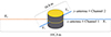 |
Fig. 2. Schematic drawing of the actively used Wind/WAVES antennas (thick blue lines) on the Wind spacecraft (grey and gold cylinder), not drawn to scale. The majority of the X+-arm was cut in 2000 and 2002 (dotted red line). |
The X+-arm was shortened by two dust impacts, first on 3 August 2000 and again on 25 September 2002 (Malaspina et al. 2014). The X−-arm and the Y±-arms remain undamaged to this day. The antenna cuts introduced significant asymmetries in the x-dipole’s differential voltage measurements, bringing it functionally closer to a monopole than a dipole antenna, though the measurements are still differential between the two antenna arms (Kellogg et al. 2016). For this reason, it is advisable to use only the dust impacts observed by the y-antenna when the signal amplitude is of interest (see Sect. 3.4.2). If only the number of impacts is of relevance, the impacts recorded by either antenna can be used. However, the response by the x-antenna to dust impacts differs before and after the antenna breaks; the two antennas do not have the same sensitivity thresholds and do not register the same amplitude distributions (see Fig. A.2). This must be accounted for.
Dust impacts on the spacecraft were measured with the fast time domain sampler (TDSF) of the Wind/WAVES instrument Bougeret et al. (1995). The TDSF sampling rate is not held constant; since April 2011 it was periodically changed every six days to a coarser sampling rate for a duration of roughly two days. When the TDSF is set to this coarse sampling rate, no dust impacts can be measured. These periodically occurring gaps must be accounted for, as is described in Appendix A.4 and evaluated in Appendix B.2.
Several other instrumental effects and external influences that affected the measurements of dust impacts occurred before 2005 (see Appendix A.1). Furthermore, the many different orbits of the Wind spacecraft, especially when changing the distance to Earth, have a noticeable effect on the observations of dust impacts (see Appendix A.5). For data analyses on time scales longer than a few weeks (e.g. the frequency analyses performed in Sect. 4) it is, therefore, advisable to use only the dust impacts observed since 2005, when Wind continuously orbited L1.
The physical processes that allow dust impact measurements via plasma wave antennas were investigated by Shen et al. (2021, 2023). These processes and the resulting signals differ for dipole and monopole antennas. Most notably, dipole antennas measure a considerably stronger amplitude when a dust particle impacts closer to the antenna’s base, unlike monopole antennas, which are not as sensitive to the distance between the impact site and the antenna’s base (Shen et al. 2023). Furthermore, the measured amplitude depends on the floating potential of the spacecraft: for a monopole antenna, a higher floating potential would not strongly affect the amplitude of the impact signal’s main peak, whereas a higher floating potential may severely reduce the amplitude of the measured main peak for a dipole antenna (Shen, M. M., priv. comm.).
3.2. Mass and speed dependence of the impact signals
The amplitude of the signal that is generated by a dust impact depends on the charge, Q, released by the impact. This charge depends on the mass, m, and the impact speed, v, of the impacting particle with respect to the spacecraft (Dietzel et al. 1973):
 (3)
(3)
A typical value for the power of the impact speed dependence is α = 3.5 (Balogh et al. 2001, Ch. 9.2), depending on the target material impacted by the dust particle (Auer 2001; Collette et al. 2014). For dipole antennas, the measured signal amplitude additionally depends strongly on the distance between the impact site and the antenna (Shen et al. 2023). The constant of proportionality, γ, is generally not known. Because only signal amplitudes above a threshold of 4 mV were considered when compiling the dataset (Malaspina et al. 2014), a faster relative speed between the spacecraft and the dust particles can lead to more detections of dust impacts: more charge is released for faster impacts, shifting the measurement threshold to lower masses.
3.2.1. Impact speed of interstellar dust particles
For ISD the impact speed depends on the orbital position of the spacecraft with respect to the ISD inflow direction and on the heliocentric speed of the ISD particle. Because ISD particles of different masses experience SRP at different strengths, i.e. because the β-ratio depends on the particle mass, the heliocentric speed of an ISD particle also depends on its mass.
This is depicted in Figs. 1a and 1b, showing the β-ratio and the heliocentric speed of an ISD particle in dependence of the particle’s mass, respectively. The β-curve has been calculated using the astronomical silicates of Gustafson (1994) rescaled to have a maximum of β = 1.6 (Sterken et al. 2013). For other materials, such as pure silicates, the β-curve can feature much lower maxima (e.g. Kimura & Mann 1999). The heliocentric speed of the dust particle has been calculated with
 (4)
(4)
where G is the gravitational constant, M⊙ is the solar mass, β is the mass-dependent β-ratio, a⊗ = 1 AU is the orbital radius of Earth, and v∞ = 26 km/s is the ISD speed at infinity. The impact speed of the particle, under the simplifying assumption that the incoming ISD velocity vector is parallel to the ecliptic plane, is
 (5)
(5)
where v⊗ ≈ 29.78 km/s is the orbital speed of Earth and ϕ is the phase of the orbit (sin ϕ = ±1 in March and September, respectively). The ISD inflow vector is not parallel to the ecliptic plane but instead inclined by about 5°, coinciding with the interstellar Helium inflow direction (Landgraf 1998; Strub et al. 2015; Swaczyna et al. 2018); this is neglected here.
Depending on the particle’s β-ratio, ISD can reach a heliocentric speed of up to 49.5 km/s (β = 0), which results in an impact speed of almost 80 km/s in March and only about 20 km/s in September. This variation of the impact speed by a factor of four becomes a factor of 128 in amplitude as per Eq. (3). Generally, the ISD particles in the relevant mass regime, m ≪ 10−9 kg, have higher β-ratios, β > 0, and, thus, lower heliocentric speeds (Fig. 1). Particles with β ≈ 0.9 have a heliocentric speed that is comparable to Earth’s orbital speed. These particles would have an impact speed of about 60 km/s in March and about 0 km/s in September, i.e. they are not measurable in September. For β > 1.38, ISD particles can no longer reach 1 AU, which corresponds to ISD particles within the mass range of mISD ∈ [1.3 × 10⁻¹⁷, 2.0 × 10⁻¹⁶] kg that cannot be observed with the Wind spacecraft throughout the year. Particles with 0.9 < β < 1.38 have a slower heliocentric speed than Earth; in September, their relative velocity vectors point in the opposite direction compared to ISD with β < 0.9.
In terms of the particle radius, assuming spherical and compact particles with a density of 2500 kg (Sterken et al. 2015), the β-gap for β > 1.38 corresponds to the radius range of a ∈ [0.11, 0.27] μm.
3.2.2. Signal amplitude of individual particle impacts
Using the mass and the mass-dependent speed of an ISD particle, the amplitude that this individual particle would generate upon impacting the Wind spacecraft can be calculated, not accounting for the unknown proportionality constant, γ, of Eq. (3). Figure 1c shows how the signal amplitude of an impacting particle changes with its mass. For IDPs, a relative speed of 20 km/s is assumed (Grün et al. 1985). The heliocentric speed of β-meteoroids can be significantly faster, commonly reaching 40 km/s (Wehry 2002, Fig. 3.15; see also Wehry et al. 2004; Zaslavsky et al. 2021); this results in impact speeds of about  because the approximately anti-sunward motion of β-meteoroids is perpendicular to Wind’s orbit (however, see Wehry & Mann 1999 for β-meteoroids that are strongly deflected from anti-sunward trajectories). The signal amplitude for impacts of ISD was calculated with impact speeds as per Eqs. (4, 5) for an impact in March and September, assuming the β-curve that is displayed in Fig. 1a.
As Fig. 1c indicates, at a given mass ISD generates a much higher signal amplitude in March than an IDP. In September, the signal amplitude of ISD is slightly lower than for an IDP at very low or very high masses (β ≈ 0), and considerably lower at intermediate masses (β > 0). Because the impact signals must exceed a certain amplitude threshold to be measured by the instrument, this should result in more detections of ISD impacts in March than in September: for a given mass, the amplitude of an ISD particle is much higher in March than it is in September; thus, in March less massive ISD particles can exceed the amplitude threshold. Furthermore, the particle flux increases with the relative speed; therefore, not only is the amplitude threshold exceeded by particles of lower mass in March compared to September, but more particles impact the spacecraft in March than in September.
There is an exception to this trend: the relative speed of ISD in September exceeds the relative speed of IDPs for 1.32 < β < 1.38 (see Fig. 1c). For β ≈ 0.9 ISD in September has almost the same heliocentric velocity as Earth; the relative speed is close to zero. The heliocentric speed of ISD in September decreases further the closer the particle is to the β-gap, β ≈ 1.38, increasing the relative speed. For 1.32 < β < 1.38 the relative speed exceeds 20 km/s; for β ≈ 1.38 the heliocentric speed of ISD is close to zero and the relative speed stems mostly from Earth’s orbital speed. The mass intervals corresponding to 1.32 < β < 1.38 are small, mISD ∈ [1.06, 1.28]×10−17 kg ∪ [2.05, 2.52]×10−16 kg, compared to the vast mass intervals with β < 1.32, and, thus, contain comparably few particles.
The time dependence of the signal amplitudes is investigated further with the aid of Fig. 3, which indicates how the signal amplitude of an impacting particle of mass m changes with the orbital position of the spacecraft, given by the month of the calendar year. As before, a relative speed of 20 km/s and 50 km/s is assumed for IDPs and β-meteoroids, respectively. No curve is visible for ISD with mISD = 10−16 kg, which cannot reach 1 AU due to its high β-ratio, and no curves were drawn for β-meteoroids above 10−16 kg due to the cutoff of their mass distribution (Wehry & Mann 1999; Moorhead 2021).
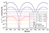 |
Fig. 3. Signal amplitude of a single dust particle, taken as m v3.5 as per Eq. (3), for an interstellar (solid curves) and interplanetary (dashed horizontal lines) dust particle and a β-meteoroid (dotted horizontal lines) of mass m = 10−18 kg (yellow lines), m = 10−17 kg (red lines), m = 10−16 kg (purple lines), m = 10−15 kg (violet lines), and m = 10−14 kg (indigo lines). The ISD with m = 10−16 kg (solid purple curve) cannot reach 1 AU due to its high β-ratio; thus, this curve is not visible. No lines were plotted for β-meteoroids above m > 10−16 kg. For more details, see Sect. 3.2.2. |
In March the ISD impact speed of up to vrel ≲ 80 km/s is considerably higher than the assumed IDP impact speed of ca. 20 km/s. Therefore, IDPs that generate signals of comparable amplitude must be much more massive. For example, to generate the same signal amplitude as an ISD particle of mISD = 10−15 kg in March, an IDP would have to be more than thirty times as massive, mIDP ≈ 4.6 × 10⁻¹⁴ kg. In September, the same ISD particle would generate a signal amplitude more than ten orders of magnitude lower than in March; it would be undetectable.
The assumed impact speed of β-meteoroids (50 km/s) is much higher than for IDPs (20 km/s), resulting in signal amplitudes that are higher by a factor of ∼25. At a mass of m = 10−17 kg the signal amplitude of a β-meteoroid can be even higher than for an ISD particle impact in March.
To summarise, due to the impact-speed-dependent amplitude threshold of the instrument, more ISD impacts are expected to be measurable when the spacecraft moves against the ISD inflow direction in March compared to when it moves with the ISD inflow in September. Section 3.4.2 will show that this seasonal variation of ISD impact detections is not apparent at all signal amplitudes, most likely due to the dissimilar mass distributions of ISD, IDPs, and β-meteoroids in the inner Solar System.
3.2.3. Mass distribution of interstellar dust and interplanetary dust particles
The mass distribution of IDPs and β-meteoroids can be described by the “Grün flux” (Grün et al. 1985): in terms of a differential mass distribution, it follows a power law, df/dm ∝ m−11/6, at low masses but features an excess with respect to that power law at masses above mIDP > 10−17 kg. This has been graphed in Fig. 4. The contribution of the β-meteoroids to the Grün flux is mostly constrained to masses below mβ < 10−16 kg; Wehry & Mann (1999) find that the mass distribution of β-meteoroids is shifted to lower masses compared to IDPs, whereas ISD was rare at these low masses at the time of this study, during the defocusing phase of the solar magnetic cycle.
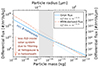 |
Fig. 4. Differential flux of IDPs following the Grün flux (solid blue curve) and ISDs derived from the MRN flux (dashed red curve). The faint dotted lines indicate the deviation from the power law df/dm ∝ m11/6. |
The differential mass distribution of ISD outside the heliosphere, the “MRN distribution” (Mathis et al. 1977), follows the same power law, df/dm ∝ m−11/6. In terms of the particle radius, this power law corresponds to df/da ∝ a−3.5. This has been graphed in Fig. 4, following the approach of Draine & Lee (1984), assuming a hydrogen number density in the ISM of nH = 0.1 cm−3, a dust particle density of 2500 kg/m3, and the heliocentric speed calculated via Eq. (4).
However, the ISD distribution is further modulated as ISD enters the heliosphere (Sterken et al. 2013), causing a notable deprivation of ISD particles below mISD ≲ 10−15 kg compared to the power law and an outright exclusion at masses below mISD ≲ 10−19 kg (Krüger et al. 2015), corresponding to particle radii of aISD ≲ 0.45 μm and aISD ≲ 20 nm, respectively. This modulation is an active research topic (e.g. Hunziker et al., in prep.; Baalmann et al., in prep.), and, thus, the mass distribution of ISD inside the heliosphere is not known with high accuracy.
To summarise, ISD is practically nonexistent in the inner Solar System at masses below mISD < 10−19 kg due to filtering at the heliopause (Slavin et al. 2012), is excluded by SRP in the β-gap of mISD ∈ [1.3 × 10⁻¹⁷, 2.0 × 10⁻¹⁶] kg, and is vanishingly rare at masses above mISD > 10−13 kg (cf. Krüger et al. 2019) due to the MRN power law distribution and the limits on cosmic dust abundances from remote observations (e.g. Frisch et al. 1999). During the defocusing phase, small ISD is furthermore defocused away from the ecliptic plane; in the focusing phase, it is focused towards it.
In contrast, IDPs follow the same power law at low masses but are not modulated by the heliopause, do not feature a β-gap, and show an excess compared to the power law at masses above mIDP > 10−17 kg; β-meteoroids are mostly constrained to mβ < 10−16 kg. While very small IDPs should also be affected by the solar magnetic cycle, these particles most likely have insufficient mass to be measurable as they impact Wind.
3.3. Dust impact database
The methodology used to compile the dataset of dust impacts on Wind is described by Malaspina & Wilson (2016). Dust impacts are identified by cross-correlating the time-resolved amplitude signal with four predetermined typical phenotypes of dust impact waveforms (types A to D; see Fig. 5): if the cross-correlation between the signal and a given morphological phenotype exceeds a given threshold, the signal is identified as a dust impact.
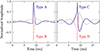 |
Fig. 5. Stylised waveforms for the four morphological phenotypes of dust impact signals measured by the TDSF. Only impacts that generated single-spike signals (left panel, types A and B) are taken into account for the analyses. Reproduced with permission after Malaspina & Wilson (2016, Fig. 2); copyright of the original figure by John Wiley and Sons. |
Morphological types A and B feature a single main peak in their waveform, whereas morphological types C and D follow the primary peak with an overshoot. The physical mechanism that causes these overshoots is not fully understood. Waveforms of type B (D) are nearly identical to type A (C) with a flipped sign, indicating that the corresponding dust impacts occurred closer to the opposite arm of the respective dipole antenna. In its current version, spanning the time period from 1995 until the end of August 2023, the dataset is publicly available on CDAWeb2.
The dataset contains the millisecond-precise timestamp of each dust impact; the peak signal amplitudes of the x-antenna and of the y-antenna, which are also referred to as Channel 1 and Channel 2, respectively; the morphological type for each channel; and a location flag that denotes whether Wind was positioned within Earth’s magnetosphere, the lunar wake, or neither.
A number of corrections were made to account for instrumental effects and similar limitations (see Appendix A.1). These are explained in detail in Appendix A and briefly summarised here:
-
Only the data since 1 January 2005 were used, when Wind continuously orbited L1. Earlier data show a geocentric distance dependence, and were affected by different data transfer rates (Appendix A.5). Both breaks of the x-dipole occurred before 2005.
-
The Wind/WAVES instrument was insensitive to dust impacts for about five months in 2013 and one month in 2014 (Appendix A.2). Spurious events measured during these time intervals were discarded within the scope of this investigation.
-
A periodic change of the TDSF sampling rate was introduced in April 2011, making the Wind/WAVES instrument insensitive to dust impacts for 45 h 36 min every six days (Appendix A.4). The full two days of data during which these measurement gaps occurred were removed.
-
The time series of dust impact signals of morphological types C and D have unexplained features, predominantly before 2005 (Malaspina & Wilson 2016); furthermore, the amplitude distribution of dust impacts of types C and D differs from those of types A and B. Therefore, only signals of morphological types A and B were taken into account. Dust impacts of types C and D are briefly investigated in Appendix B.6.
-
When investigating the amplitude distribution of the dust impact signals (Sect. 3.4.2), only dust impacts measured by the y-antenna were taken into account (see Fig. A.2).
3.4. Overview of dust impacts at L1
An overview of the observed dust impacts on Wind at L1 that generated signals of morphological types A and B, spanning the time interval from 1 January 2005 to 31 August 2023, is given in Fig. 6a. Because the number of dust impacts shows a strong stochastic day-to-day variation, it is expedient to view a moving average of the data. A window width of a quarter year has proven to be a reasonable compromise between smoothing out the random variations without inadvertently suppressing long-term patterns.
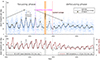 |
Fig. 6. Dust impacts observed by Wind versus time. Top panel: Daily number of dust impacts on Wind at L1 that generated signals of morphological types A and B, given for each day (blue discs) and as a centred moving average with a width of 91 d (black line). For comparison, yellow diamonds mark the moving average flux on 25 March of each year, which is close to each annual maximum. The sampling rate was periodically changed beginning in April 2011, marked by a vertical dotted pink line, making the instrument insensitive to dust impacts for roughly two days every six days. Larger time periods where the instrument was inoperable in regard to measuring dust impacts occurred in 2013 (shaded orange, “z-trigger”) and in late 2014 (shaded red, “system outage”). The increase and decrease of dust impacts due to the solar magnetic cycle is indicated by diagonal grey arrows. The dataset has been corrected for these instrumental effects as per Sect. 3.3 (see Appendix A). Bottom panel: Daily number of dust impacts observed by Wind as a 91 d centred moving average (black curve, identical to the top panel) compared to the numerically simulated particle flux of ISD at Wind’s orbital position, vertically offset by an assumed constant IDP flux of 10 #/d. (For more information on the simulations, see Sect. 3.4.1). |
On top of a roughly constant level of about 12 impacts per day, these long-term patterns are dominated by a seasonal variation: in March of each year, dust impact detections occur at a higher rate compared to September of the same year. This corresponds to the orbital position of Wind with respect to the inflow direction of ISD; the spacecraft moves against the ISD inflow in March and with it in September of each year (cf. Malaspina et al. 2014, Fig. 4). A higher relative speed between the spacecraft and the ISD in March of every year directly results in a higher observed particle flux. Furthermore, as per Eq. (3), a faster relative speed can increase the signal amplitude that is measured by the instrument by multiple orders of magnitude, allowing for the detection of lower-mass particles that would otherwise not produce signal amplitudes above the instrument’s detection threshold (Fig. 3).
IDPs revolve around the Sun on mostly prograde elliptical orbits and are not expected to show this seasonal variation. However, the plane of symmetry of IDPs is slightly inclined by 3.7° ±0.6° with respect to the ecliptic plane (Leinert et al. 1976). Furthermore, Earth and Wind encounter meteoroid streams typically once or twice per orbit per stream. These annual effects are assumed to be negligible compared to the seasonal variation stemming from Wind’s relative velocity with respect to the ISD inflow direction. Therefore, the seasonal variation is attributed to ISD.
The seasonal variation itself varies on a decadal time scale: it is strongest around the solar minimum of December 2008 and weakest around the solar minimum of December 2019, corresponding to the focusing and defocusing phases of the solar magnetic cycle. The lower envelope of the seasonal minima roughly forms the previously noted horizontal level of about 12 impacts per day, which was identified as the interplanetary component of the dust population, whereas the seasonal and decadal variations are mainly associated with the interstellar component (see Sect. 3.4.1). It is, unfortunately, not yet possible to identify an individual impacting particle as interplanetary or interstellar.
3.4.1. Comparison with numerical simulations
Fig. 6b compares the observed daily number of dust impacts with a numerically simulated cosmic dust particle flux at Wind’s orbital position. The numerical simulations were performed with the IMEX code (Sterken et al. 2012; Strub et al. 2019), which models ISD under the influence of solar gravity, SRP, and the Lorentz force, assuming a Parker spiral IMF that is modulated with the solar magnetic 22 yr-cycle. Simulated ISD particles were launched at a distance of 50 AU upstream of the Sun; the model does not yet include the outer heliosphere and, thus, does not yet include the filtering effects by the heliosheath (e.g. Slavin et al. 2012; Sterken et al. 2013).
ISD trajectories were computed for spherical compact particles with a density of 2500 kg/m3 and radii of a ∈ {0.30, 0.41, 0.54, 0.73} μm, assuming adapted astronomical silicates with a maximum β-ratio of βmax = 1.6 (Gustafson 1994; Sterken et al. 2013); see also Fig. 1. The resulting flux densities at the modelled particle sizes were integrated over a MRN-like power law size distribution with an ISM hydrogen number density of nH = 0.1 cm−3 (Mathis et al. 1977); confer Sect. 3.2.3.
The assumption of a MRN-like power law size distribution motivated the cutoff of the modelled size distribution below amin = 0.3 μm: slightly smaller particles, a ∈ [0.1, 0.3] μm cannot reach the Wind spacecraft because they are excluded by SRP (see Sect. 3.2.3), assuming the same β-curve as in Sect. 3.2.1, and even smaller particles, a < 0.1 μm, were excluded as a simplification of the heliosheath filtering. Although Ulysses observed ISD particles down to masses of ∼10−18 kg, corresponding to particle radii of a few tens of nanometres, the observed ISD size distribution was strongly depleted at these particle radii compared to a MRN distribution (Krüger et al. 2015).
The particle flux was calculated by multiplying the integrated flux density with the surface area of the detector, which was assumed to be the apparent cross-section of Wind’s cylindrical body, 1.8 m × 2.4 m = 4.32 m2 (see Hervig et al. 2022). A constant IDP flux of 10 #/d was assumed, resulting in the simulated particle flux that is shown in Fig. 6b.
These numerical simulations are not intended for a detailed comparison with the observed dust impacts: for example, the modelled particle flux does not take into account the signal amplitude threshold of the Wind/WAVES instrument and, thus, is not identical to the expected number of dust impact detections. Nevertheless, although these numerical simulations are simplified, they successfully reproduce the decadal variation due to the solar magnetic 22 yr-cycle and the seasonal variation due to the spacecraft’s orbit.
3.4.2. Dust impact observations at different signal amplitudes
The long-term patterns in the daily number of dust impacts that are presented in Fig. 6 are not equally present at all signal amplitudes. As per Eq. (3), the signal amplitude that is generated by an impacting dust particle depends on the particle’s mass and impact speed. However, because the mass and the impact speed cannot be disentangled from the signal amplitude, it is not known to which mass range the instrument is sensitive.
Empirically, the long-term patterns in the daily number of dust impacts look starkly different for the weakest and the strongest signal amplitudes. This is shown in Fig. 7, which presents the time series for all dust impacts with signal amplitudes below 19.2 mV and above 240 mV, corresponding to the weakest and strongest 20% of all signals measured by the y-antenna (Channel 2) with morphological types A and B.
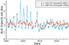 |
Fig. 7. Time series for all dust impacts of morphological types A and B with a y-antenna signal amplitude below 19.2 mV (blue) and above 240 mV (red), graphed as a centred moving average with a width of 91 d. The two amplitude selections each correspond to 20% of all impacts. |
As Fig. 7 shows, the seasonal variation that was noted for the full dataset (see Fig. 6a) is readily apparent for the weakest signal amplitudes, showing an annual maximum of daily dust impacts in March and an annual minimum in September. This seasonal variation is stronger before 2015, during the focusing phase of the solar magnetic cycle, than since 2015, in the defocusing phase. In contrast, for the dust impacts that generated the strongest signal amplitudes, Fig. 7 shows a near-constant if noisy level of about two daily impacts with no clear evidence of the seasonal variation. Because the seasonal variation is attributed to ISD, this implies that a significant fraction of the measured impacts with the weakest amplitudes are caused by ISD, whereas the strongest signal amplitudes are presumably mainly caused by impacts of IDPs.
This is supported by the distribution of the signal amplitudes of the impacts measured by the y-antenna (Channel 2), which is displayed in Fig. 8. In the orbital segment where the spacecraft moves against the ISD inflow direction (February to April), an excess of weak-amplitude signals is observed compared to the orbital segment where the spacecraft moves with the ISD inflow direction (August to October). This excess is identified as ISD. Above an amplitude of A ≳ 200 mV the distributions for both orbital segments are similar; Fig. 7 shows almost no seasonal variation for signal amplitudes A > 240 mV.
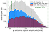 |
Fig. 8. Amplitude distributions of all impacts (grey bars) with morphological types A and B measured by the y-antenna, impacts measured only when the spacecraft moved against the ISD inflow direction during February, March, and April (shown with blue filled bars outlined in white), and impacts measured only when the spacecraft moved with the ISD inflow direction during August, September, and October (shown with red filled bars outlined in black). The distribution of all impacts has been scaled by a factor of 0.5 to tighten the histogram’s vertical axis. The vertical dashed green lines indicate every 20th percentile of the signal amplitude; the weakest and the strongest 20% of all impact signals were selected when generating Fig. 7. |
This gives rise to the following hypothesis: the measured ISD-to-IDP ratio decreases with increasing signal amplitude. In the amplitude range above A ≳ 200 mV virtually no impacts from ISD were registered, whereas in the amplitude range below A ≲ 20 mV the number of impacts during February to April is roughly twice as high as during August to October.
Because ISD is much faster than IDPs in March and generally slower in September, this implies that the excess at weak amplitudes in March is caused by low-mass ISD that does not generate sufficiently strong signal amplitudes to be measurable in September; furthermore, a lower particle flux due to a lower relative speed also reduces the number of impacts per time. That the signal amplitude distribution looks similar at strong amplitudes for both investigated orbital segments of Fig. 8 implies that very little ISD of sufficiently high mass and velocity to generate these signal amplitudes exists. However, because IDPs are generally slower in March than ISD, this implies that the strong-amplitude impacts are generated by even higher-mass IDPs, i.e. there must be a considerable excess of the IDP mass distribution at high masses compared to ISD. An alternative explanation could be a second population of IDPs that is considerably faster but not considerably less massive than the first IDP population. A candidate can be β-meteoroids, which often feature slightly lower masses but much faster speeds than other IDPs (Sects. 3.2.2 and 3.2.3).
In particular, for the mass range around m ≈ 10−17 kg the signal amplitudes of β-meteoroids are similar to ISD in March (Sect. 3.2.2). At slightly higher masses, ISD is excluded by the β-gap but IDPs and β-meteoroids are not (Sect. 3.2.3). This may indicate that the dust impact observations are predominantly caused by ISD and β-meteoroids of this mass regime.
In order to investigate this further, it would be essential to know the impact speed and mass of a measured particle impact, necessitating a mission at 1 AU with a more elaborate dust detector. Knowledge of the direction of origin of an impacting dust particle would allow for better differentiation between ISD, β-meteoroids, and other IDPs. A dedicated dust detector on the Lunar Gateway (Wozniakiewicz et al. 2021; Arnet 2023; Sterken et al., in prep.) or the proposed SunCHASER mission (Posner et al. 2021; Cho et al. 2023) would therefore be of great benefit. Nevertheless, this analysis indicates that the ISD impacts observed by Wind are primarily associated with weak-amplitude signals, and that strong-amplitude impacts are predominantly caused by IDPs.
4. Frequency analysis
Frequency analysis has been performed on the dataset of dust impacts at L1, which covers the time range from 2005 to the end of August 2023. This dataset contains two long-term gaps in the data and many periodically occurring 2 d-long gaps since April 2011 (see Sect. 3.3).
Therefore, the resulting time series is no longer evenly sampled, and the necessary assumptions for the discrete Fourier transform (DFT) are not met. The most common alternative to DFT for unevenly spaced data, the Lomb-Scargle transform (Lomb 1976; Scargle 1982), can suffer from phase and amplitude artefacts (e.g. Foster 1995; Cumming et al. 1999). Instead, the method proposed by Kirchner & Neal (2013, Suppl. Mat.), which is based on the date-compensated discrete Fourier transform (DCDFT; Ferraz-Mello 1981), is used. Consistent results are also obtained from Kirchner and Neal’s implementation of the Weighted Wavelet Z transform (Foster 1996), which additionally suppresses spectral aliasing that can arise from uneven sampling. These methods are presented and evaluated in Appendix B.
Within this investigation the periodogram amplitude was calculated by Kirchner & Neal’s DCDFT-based method at each frequency on an equidistant frequency grid. This grid corresponds to the natural frequencies of a DFT oversampled by a factor of 15, increasing the number of frequencies at which the spectrum is evaluated by that factor of 15 compared to a DFT. The data were linearly detrended before calculating the spectrum. The 95% significance thresholds of each respective spectrum were estimated by the 95th percentile of periodogram amplitudes for randomly resampled time series (see Appendix B.1): the probability of a random noise peak at the respective frequency reaching this threshold is 5%; thus, the statistical significance of a peak that reaches the threshold is 95%, and higher peaks are more significant.
4.1. Discovery of solar rotation signatures
The periodogram of the daily dust impacts with morphological types A and B recorded at L1 is presented in Fig. 9. For easier comparison, the most relevant periods and their harmonics have been marked.
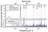 |
Fig. 9. Periodogram of the daily number of dust impacts with morphological types A and B recorded at L1. The periodogram was evaluated at the DFT’s natural frequencies and oversampled by a factor of 15. The three most relevant frequencies and their harmonics are marked by vertical lines: the 365 d-period corresponding to the orbital period of the spacecraft (dotted green lines), the 6 d-period introduced by instrumental effects (dashed purple lines), and the solar rotation period at 27 d (solid brown lines). The bottom panel shows a zoomed-in view of the full spectrum with the estimated 95% significance thresholds indicated by a grey shaded area. |
The spectrum’s most powerful peak lies at 364 d; its first harmonic at 182 d also has a considerable power. These features correspond to the revolution of the Wind spacecraft around the Sun and the seasonal variability reported in Sect. 3.4: once per orbit, the spacecraft moves against the inflow direction of ISD, and once per orbit it moves with this direction. Because no dependence on the direction of motion of the spacecraft is known for IDPs, these spectral features are caused almost entirely by ISD.
Another powerful spectral feature comes from the periodic change of the sampling rate, which leads to the removal of two days of dust data every six days since April 2011 (see Appendix A.4). This spectral peak is observed at 5.99 d, and its first harmonic lies at 3.02 d. These two periods have been marked in the figure by dashed lines.
Three more spectral peaks are evident in the data and are interpreted as signatures of the solar rotation. This marks the first discovery of solar rotation signatures in cosmic dust data. The most powerful and most clearly defined peak lies at 9.01 d and is identified as the second harmonic of a 27 d period. Another clearly defined peak lies at 13.5 d and is identified as the first harmonic of the same. There is no notable spectral peak at precisely 27 d; however, a broader peak at 26.4 d is present. The frequency resolution of the periodogram of Fig. 9 is 1.5 × 10⁻⁴ d−1, which corresponds to roughly 0.11 d in the period range at 27 d; the displacement of the peak from 27 d to 26.4 d is thus not an effect of the frequency resolution.
The origin of the solar rotation signatures is investigated further by determining:
-
whether the solar rotation signatures are caused by the interstellar or by the interplanetary dust population (Sect. 4.2);
-
whether the solar rotation signatures are created through CIRs (Sect. 4.3);
-
whether the solar rotation signatures are created through the IMF sector structure or crossings of the heliospheric current sheet (Sect. 4.4); and
-
whether the solar rotation signatures are not genuine signatures of the dust environment but created through periodic external effects (Sect. 4.5).
4.2. Interstellar versus interplanetary dust
There are two primary selection methods that can help distinguish an ISD population from an IDP population. First, much more ISD is detected when the spacecraft moves against the ISD inflow direction in March than when it moves with the ISD inflow direction in September. Thus, if the solar rotation signatures are more powerful in the early calendar year than in the late calendar year, summed over all years, they should be caused, at least partially, by ISD. If they have the same power throughout the year, they should be caused predominantly by IDPs (see Sect. 4.2.1).
Second, the ecliptic plane contains much more ISD during the focusing phase of the solar magnetic cycle than during the defocusing phase, whereas the population of measurable IDPs appears to be not as strongly affected by the solar magnetic cycle (see Fig. 7 and Sect. 3.4.2). Thus, if the solar rotation signatures are much stronger during the focusing phase than during the defocusing phase, they should be caused, at least partially, by ISD. If they are of comparable power in both phases, they should be caused predominantly by IDPs (see Sect. 4.2.2).
4.2.1. Against versus with the interstellar dust inflow direction
Figure 10 displays a comparison of the power spectra of the daily number of dust impacts with morphological types A and B during the orbital segments against or with the ISD inflow direction, respectively. For the respective dataset, all data outside a quarter orbit, corresponding to the months of February to April when going against the ISD inflow and August to October when going with the ISD inflow, were removed before calculating the spectra. This receiver function, which is one during the selected quarter orbit and zero during the remaining three-quarters of the orbit, is visible in the harmonics of the 365 d-period that decline in power with decreasing period. The convolution of the dust impact time series with this receiver function significantly diffuses the spectral peaks. It also causes the estimated 95% significance threshold to drop to a lower value at a period of 365 d and its harmonics.
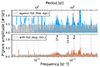 |
Fig. 10. Periodograms of the daily number of dust impacts with morphological types A and B for the three months of each year that correspond either to the orbital segment against the ISD inflow (February to April, blue curve, top panel) or with the ISD inflow direction (August to October, red curve, bottom panel). The two panels are scaled identically; the estimated 95% significance thresholds are indicated by grey shaded areas. Frequencies of interest are marked by vertical lines as in Fig. 9. |
Both spectra show evidence of the solar rotation signatures. All three solar rotation peaks are more powerful by about a factor of three when going against the ISD inflow than when going with the ISD inflow, which indicates that the solar rotation signatures are not exclusively present in IDPs but are, at least in large part, caused by ISD.
4.2.2. Focusing versus defocusing phase
Figure 11 shows a comparison of the power spectra of the daily number of dust impacts with morphological types A and B during the focusing phase (2007 to 2012) and during the defocusing phase (September 2017 to August 2023), respectively. The seasonal variation (365 d-peak) is more powerful by roughly an order of magnitude during the focusing phase, indicating that more ISD is measured in addition to IDPs during the focusing phase. The instrumental 6 d-peak is more powerful during the defocusing phase because it affected the instrument only since April 2011 (Sect. 3.1).
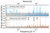 |
Fig. 11. Periodograms of the daily number of dust impacts with morphological types A and B during six years in the focusing phase (2007–2012, blue curve, top panel) and six years in the defocusing phase (September 2017 to August 2023, red curve, bottom panel). The two panels are scaled identically; the estimated 95% significance thresholds are indicated by grey shaded areas. Frequencies of interest are marked by vertical lines as in Fig. 9. |
During the focusing phase, clear and powerful spectral peaks can be observed at 13.5 d and 9 d. Another peak at ∼27 d is less powerful and more diffuse.
During the defocusing phase, these solar rotation signatures are less prominent and may vanish. For example, the first harmonic is diminished by a factor of about two, and the second harmonic is not perceptible above neighbouring noise peaks. Furthermore, the spectral peaks that are perceptible do not align exactly with the periods of interest but appear slightly shifted.
In conclusion, the solar rotation signatures are clearer and more powerful during the focusing phase than during the defocusing phase, indicating that they are caused, at least in large part, by ISD. A caveat to this analysis is that not only ISD but also low-mass IDPs could be affected by the solar magnetic cycle, for example β-meteoroids or nanodust.
4.3. Influence of co-rotating interaction regions
Because the spacecraft encounters CIRs at the solar rotation period of about 27 d, CIRs are the primary contender to explain the origin of the solar rotation signatures. The higher solar wind speed, stronger IMF, and charging effects due to higher plasma temperatures during CIRs compared to the average solar wind (Hajra & Sunny 2022) result in a stronger Lorentz force that may deflect submicron-sized dust; these dust particles may be charged even more due to their fluffiness (Ma et al. 2013).
Flandes et al. (2011) and Hsu et al. (2010) found that CIRs can periodically affect dust in the Jovian and Saturnian environment, respectively. The particles of these dust streams were identified to be around ∼10 nm in radius (Zook et al. 1996; Hsu et al. 2011). However, Malaspina et al. (2014) estimate from the observed IDP flux that Wind is sensitive to impacts of approximately submicron-sized dust particles; Kellogg et al. (2016) conclude that Wind is insensitive to impacts of highly accelerated nanodust. Thus, particles that are comparable in size to Jovian and Saturnian dust streams are unlikely to be detectable by Wind. Moreover, the mechanism that causes the Jovian and Saturnian dust streams can act on particles with radii of ∼10 nm but is not expected to extend to submicron-sized dust (Hsu et al. 2010).
St. Cyr et al. (2017) report a reduction of dust impact detections by Wind during CMEs. Calculations by Ragot & Kahler (2003) find that dust particles with radii of between ca. 0.1 μm and 3 μm can be depleted by CMEs in the solar corona3. Simulations by Wagner & Wimmer-Schweingruber (2009) indicate that dust particles with radii up to 1 μm may be perturbed by CMEs as they get closer to the Sun than 1 AU by Poynting-Robertson drag. Similar perturbation effects on dust particles in this size range may also be induced by SIRs. This motivates a superposed epoch analysis of dust impact detections during SIRs.
4.3.1. Superposed epoch analysis of stream interaction regions that are associated with co-rotating interaction regions
Figure 12a shows a superposed epoch analysis (Chree 1913) of the daily number of dust impacts for all SIRs that are associated with CIRs from the datasets by Jian et al. (2006), Jian (2021) and Hajra & Sunny (2022) since 2005. SIRs that are not associated with CIRs were not taken into account because non co-rotating SIRs are unrelated to the solar rotation period. The time intervals of the SIRs were rescaled to the duration of the respective SIR before superposition. More details of the methodology are presented in Appendix C.
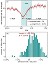 |
Fig. 12. Reduction and enhancement of dust impact detections made by Wind during SIRs. Top panel: Scaled superposed epoch analysis of the daily number of dust impacts during SIRs as a moving average within a 30 min interval (grey) or a 4 h interval (red). Only the SIRs that are associated with CIRs were taken into account. The shaded red area indicates 95% confidence intervals for a Poissonian distribution. Bottom panel: Histogram of the enhancement or reduction factor of dust impacts for the SIRs that are associated with CIRs. The dashed blue line denotes the average reduction of 20.7%. The five SIRs that begin on 1 January 2005, 23 November 2006, 15 January 2007, 24 November 2008, and 30 August 2009 were excluded due to low number statistics. |
As Fig. 12a indicates, on average, a reduction of dust impacts is observed during these SIRs compared to the preceding and following time periods: dust impact detections are reduced, on average, by 23.8%±2.4% during these SIRs compared to the preceding and following time periods. This reduction appears to begin a few hours before the start of the superposed SIR and is more pronounced during the first half of the superposed SIR compared to the second half.
Figure 12b shows that SIRs can feature either a reduction or an enhancement of dust impact detections compared to the preceding and following time intervals. However, this distribution is shifted towards a reduction of dust impact measurements during SIRs: only 82 SIRs of the dataset feature an enhancement, whereas 398 SIRs feature a reduction. On average, the SIRs reduce the number of dust impact detections by 21% with a standard deviation of 26%.
The difference in the average strength of dust impact reduction, 23.8% in the superposed epoch analysis and 21% in the histogram, stems from the difference in methodology: the superposed epoch analysis sums the number of dust impacts over all SIRs, i.e. the sum is naturally weighted by the number of dust impacts during the respective SIR. In the histogram, each SIR is assigned the same weight.
The effect of the 82 SIRs that cause an enhancement of dust impact detections was investigated: artificial gaps were induced in the dust impact time series whenever one of these “enhancing SIRs” occurred, beginning three days before the start of the respective SIR and ending three days after the end of each SIR, i.e. about a week of data surrounding each enhancing SIR was removed. The periodogram of this modified time series does not significantly differ from the periodogram of the original time series (Fig. 9). This indicates that the solar rotation signatures are not associated with only the SIRs that enhance the number of detections of dust impacts. This is important for rejecting the hypothesis that the solar rotation signatures are caused by instrumental effects (see Sect. 4.5.1).
When performing the same investigation for the 398 SIRs that reduce the dust impact observations, the solar rotation signatures were strongly diminished. This indicates that the solar rotation signatures are associated with these “reducing SIRs”. Most likely, both the enhancing and the reducing SIRs cause the solar rotation signatures; however, because there are far fewer enhancing SIRs than reducing SIRs, the effect of their removal on the spectrum is comparably minor.
Péronne et al. (in prep.) investigate how the reduction or enhancement of dust impact detections varies with the properties of the respective SIRs or CMEs, for example with the IMF strength or the presence or absence of interplanetary shocks. Further modelling efforts are required to probe the physical mechanism of this reduction of dust impacts during SIRs. Observations with a dust detector that can determine the particles’ masses, such as an impact ionisation detector, would be essential in confirming the size range of the affected dust particles.
4.3.2. Dust spectra for time intervals that are rich and poor in co-rotating interaction regions
To investigate whether the solar rotation signatures are related to CIRs, time intervals with different rates of occurrence and CIR durations were analysed. If the solar rotation signatures are related to CIRs, they should be more powerful during time intervals where multiple long-lasting CIRs occurred and less powerful during time intervals where no or only short-lasting CIRs occurred.
The datasets by Jian et al. (2006), Jian (2021) and Hajra & Sunny (2022) list individual SIRs. While the dataset by Jian et al. (2006), Jian (2021) flags whether a SIR is associated with CIRs in general, it does not indicate which individual SIRs are recurrences of the same co-rotating structure. It is therefore necessary to identify CIRs in these datasets. The method of CIR identification is detailed in Appendix B.4 and assesses whether two SIRs that could be part of a CIR are separated in time by the solar rotation period.
The resulting list of CIRs is displayed in Fig. 13, showing the time interval that is covered by each CIR. Dumbović et al. (2022) found a CIR that lasted for 27 Carrington rotations from June 2007 to May 2009. The CIRs displayed in Fig. 13 do not include this single long-lasting CIR, but do include two similarly long-lasting CIRs in 2008.
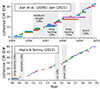 |
Fig. 13. CIRs identified by the method proposed in Sect. 4.3.2 for the SIR datasets of Jian et al. (2006), Jian (2021) since 2005 (top panel) and Hajra & Sunny (2022) (bottom panel). Each horizontal bar corresponds to one CIR. Time intervals of interest have been highlighted by shaded areas. We note that the two datasets overlap only for the years 2008 and 2009. |
Six time intervals of interest were selected on the basis of Fig. 13. For easier comparison, each time interval was selected to be nine months long. These time intervals of interest, given by the day-of-year (doy) are:
-
(a)
2006 doy 91–365, when multiple CIRs that each last a few months were identified;
-
(b)
2007 doy 1–273, when at least two long-lasting CIRs were observed;
-
(c)
2008 doy 1–273, when two extremely long-lasting CIRs were identified, coincident with the long-lasting CIR observed by Dumbović et al. (2022);
-
(d)
2009 doy 1–273, when many short-lasting CIRs were identified in the dataset by Jian et al. (2006), Jian (2021) and very few CIRs were identified in the dataset by Hajra & Sunny (2022);
-
(e)
2014 doy 23–295, when no CIRs were identified; and
-
(f)
2015 doy 23–295, when many short-lasting CIRs were identified.
Periodograms have been generated for these particular time periods. Figure 14 (left column) presents three of these time periods: (c) 2008, when two long-lasting CIRs were identified; (e) 2014, when no CIRs were identified; and (f) 2015, when many short-lasting CIRs were identified.
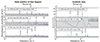 |
Fig. 14. Periodograms for certain time periods corresponding to different systematic rates of occurrence of CIRs for the daily number of dust impacts with morphological types A and B (left, indigo curves) and of a synthetic time series of dust impacts with an absolute dust depletion by SIRs (right, teal curves; see Sect. 4.3.3). All of the selected time periods are nine months long; their initial and final dates are given as doy. All panels in the left column share the same axis range and scale for easier comparison. The panels in the right column are scaled differently. Frequencies of interest are marked by vertical red lines as in Fig. 9, including the third solar rotation harmonic at 6.75 d; the 6 d-periodicity has only been marked in the dust impact spectra since 2011. Estimated 95% significance thresholds are indicated by grey shaded areas. |
The solar rotation signatures were most easily identifiable when long-lasting CIRs occurred in 2008 (c) and in 2007 (b, not depicted). At times where no CIRs (e, 2014) or multiple short-lasting CIRs (f, 2015; also a and d, 2006 and 2009, not depicted) were identified, the solar rotation signatures were weaker.
This suggests that the detected solar rotation signatures are connected to CIRs. That long-lasting CIRs cause more powerful solar rotation signatures is reasonable: a long-lasting periodic signal, i.e. one long-lasting CIR, causes a stronger spectral peak at the relevant period than multiple short-lasting periodic signals that are individually time-offset, i.e. multiple short-lasting CIRs. A periodic signal that consists of multiple peaks in time can generate a spectrum that is more powerful at the harmonics than at the primary (see Appendix B.3), which explains why different spectra exhibit different relative amounts of periodogram amplitude in the harmonics.
4.3.3. Synthetic data of dust impacts depleted by co-rotating interaction regions
To further evaluate the hypothesis that the solar rotation signatures are caused by CIRs a synthetic time series of observed dust impacts on Wind was constructed. This synthetic time series describes the daily number of dust impacts, N, as a function of time, t, by
 (6)
(6)
and is displayed in Fig. 15. It consists of a constant rate of NIDP = 12 IDP impacts per day; the ISD rate periodically changes with the solar magnetic cycle of 22 yr and the spacecraft’s orbital period of 1 yr, with a maximum of NISD = 18 ISD impacts per day (see Sect. 3.4). The effect of the solar magnetic cycle on the dust has its maximum during solar minimum (Landgraf 2000; Sterken et al. 2012), here taken as tmin = 1 December 2012; and the seasonal cycle has its maximum when the spacecraft moves against the ISD inflow direction, here taken as tag = 15 March 2015. The synthetic time series was constructed to reproduce the large-scale variations indicated in Fig. 6a and is not physically motivated.
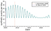 |
Fig. 15. Synthetic time series of IDP and ISD impacts on Wind following Eq. (6) to reproduce the observed number of impacts in Fig. 6a. The times at which the oscillations due to the solar magnetic cycle and the annual variation are at their maxima are indicated by a vertical dashed red line and a vertical dotted purple line, respectively. |
The effect of SIRs was tested by setting the synthetic time series to zero during a SIR, N(ti) = 0 ∀ti ∈ SIR. This was carried out for all SIRs, not only those that were identified as part of a CIR. This absolute local depletion of dust by a SIR is not intended to be physical; this exaggeration of the effect was chosen to better investigate how the spectrum is influenced.
In analogy to Sect. 4.3.2, the case studies of time periods that are of interest with respect to the occurrence of CIRs were repeated for this synthetic time series with dust depletion by SIRs. A selection of the resulting spectra is shown in Fig. 14 (right column).
The peaks in the synthetic data spectra are not identical to those found in the genuine spectra but correspond reasonably well. In particular, for the time period in 2008 when long-lasting CIRs were identified (c), the spectral features are similar for both spectra, and the solar rotation signatures are evident in both the genuine dust spectrum and in the synthetic data spectrum. The spectra for the fairly short-lasting CIRs in 2006 and 2009 (a and d; not depicted) match similarly.
In the 2014 time period where no CIRs were observed (e), neither the spectrum of the genuine dust impacts nor that of the synthetic data show strong solar rotation signatures. The weak spectral peak in the synthetic data periodogram at approximately 9 d is caused by two non-CIR SIRs that are separated by 9 d; it lies below the estimated 95% significance threshold and is not a signature of the solar rotation. For the many short-lasting CIRs of 2015 (f), both the genuine data and the synthetic data feature only one strong peak adjacent to the solar rotation period and minor peaks at the first and third harmonics.
We note that the genuine and the synthetic spectra do not always fully agree, which may be due to, for example, variations of the CIR parameters, such as the IMF strength, that cause variations in the strength of the observed reduction of dust (see Fig. 12b). Nevertheless, the similarities between the spectra of the synthetic data and of the genuine dust impact data suggest a close relation between CIRs and solar rotation signatures in the dust: it appears that most CIRs locally reduce the number of dust impacts that are observed by the spacecraft at 1 AU as it is passed by the individual CIR.
4.4. Influence of the interplanetary magnetic field sector structure
An individual crossing of the HCS by the spacecraft is unlikely to have much of an effect due to the time scale: Liou & Wu (2021) report an average thickness of the HCS of about 105 km with a maximum thickness of about 106 km. The orbital speed of Earth – and, thus, of the spacecraft – around the Sun is about 30 km/s. Thus, it would take the spacecraft a few hours to cross a highly inclined HCS. This is a considerably shorter time scale than the duration of a passing SIR (∼36 h; Jian et al. 2006). Similarly, the strength of the IMF varies by perhaps 20% as the spacecraft crosses the HCS (Liou & Wu 2021), whereas a SIR enhances the magnetic field much more strongly (on average by a factor of two to three; e.g. Geyer et al. 2021; Hajra & Sunny 2022). Thus, the crossings of the HCS are unlikely to have a strong effect on dust particles compared to SIRs. However, the alternating sector structure of the IMF may play a much larger role than individual spacecraft crossings of the HCS.
The alternating polarity of the magnetic field in adjacent sectors of the IMF was proposed as the cause of the periodic appearance of Jovian dust streams (Hamilton & Burns 1993). However, Flandes et al. (2011) find a strong correlation between Jovian dust streams and the compression regions of, for example, CIRs. Similarly, Hsu et al. (2010) find that Saturnian dust streams result from the combination of both CIRs and the alternating sector structure.
It is therefore unlikely that the sector structure alone is the sole cause of the solar rotation signatures. Case studies similar to Sect. 4.3.2 were performed to confirm or refute this hypothesis, making use of the dust impact data and of the daily IMF polarity data given by Svalgaard (2023b). This is presented in detail in Appendix B.5.
The spectra of the IMF polarity data (see Fig. B.5, right column) are highly correlated to the IMF sector structure stability: they feature strong 27 d-peaks for a two-sector structure and strong 13.5 d-peaks for a four-sector structure, and the solar rotation signatures in the IMF polarity data are weakened during times of a chaotic sector structure. In contrast, the dust impact spectra (see Fig. B.5, left column) do not show this correlation: for example, during a stable four-sector structure, a powerful 27 d-peak and a weak 13.5 d-peak are observed; and the solar rotation signatures can be powerful during a chaotic IMF sector structure and weak during a stable IMF sector structure.
This indicates that the alternating polarities of the IMF sector structure are not the sole cause of the solar rotation signatures. However, this only holds true for the local sector structure at the spacecraft; ISD travelling through the heliosphere may nevertheless experience alternating phases of focusing and defocusing with respect to the ecliptic plane as it encounters the alternating polarities of the IMF sector structure. Similarly, dust may be affected differently when CIRs and HCS crossings coincide, as is the case farther away from the Sun, for example in Jupiter’s or Saturn’s orbits (Gosling & Pizzo 1999). Nevertheless, while the local IMF sector structure is expected to affect cosmic dust, it is unlikely to be the sole cause of the observed solar rotation signatures.
4.5. Influence of external effects
It may be possible that the solar rotation signatures in the dust impact data do not reflect a genuine pattern in the dust environment but are artificially caused by external effects. One of these external effects is a periodic change of the spacecraft’s floating potential when encountering CIRs (Sect. 4.5.1); another external effect is a periodic insensitivity to dust impacts upstream of interplanetary shocks associated with CIRs (Sect. 4.5.2). The influence of these two potential artificial origins of the solar rotation signatures are investigated below.
4.5.1. Influence of the spacecraft’s floating potential
Wilson et al. (2023a) report evidence of solar rotation signatures in the floating potential of the Wind spacecraft and hypothesise that CIRs are the origin. Thus, one must consider that the solar rotation signatures in the dust impact spectra may not stem from a genuine reduction of dust impacts as suggested in Sect. 4.3.1; instead, periodic changes of the spacecraft floating potential could artificially induce these signatures by periodically reducing the instrument’s sensitivity to dust impacts.
The dataset of Wilson et al. (2023b), using the spacecraft potential derived by the local minimum of the electron energy distribution function with parallel pitch-angles as in Wilson et al. (2023a, Fig. 6), yields the power spectrum displayed in Fig. 16. Spectra for the spacecraft potential derived with different methods of Wilson et al. (2023a) are quantitatively but not qualitatively different. High periodogram amplitudes are observed at the primary and the first two harmonics of the solar rotation period; the third harmonic is less powerful but still notable. These solar rotation signatures are much more prominent in the spacecraft potential spectrum than in the dust impact spectrum (see Fig. 9).
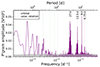 |
Fig. 16. Periodogram of Wind’s floating potential from 2005 to 2021 using Method 4 of Wilson et al. (2023a) for parallel pitch angles (cf. Wilson et al. 2023a, Fig. 6). The data were averaged over each day before generating the spectrum. The vertical lines are as in Fig. 9. The estimated 95% significance thresholds are indicated by a grey shaded area. |
The question remains whether the change of the spacecraft floating potential during a CIR decreases the instrument’s sensitivity to dust impacts, artificially inducing a reduction of observed dust impacts, or if it increases the instrument’s sensitivity, counteracting a genuine reduction of dust impacts. Within a CIR the plasma density is increased compared to the surrounding interplanetary medium (Sect. 2.4). This density enhancement increases the electron thermal current Wind experiences, decreasing the spacecraft’s floating potential to lower positive values (Garrett 1981). The spacecraft’s charging timescales of tens of milliseconds are negligible compared to the duration of the CIRs of a few days (Chen et al. 2013; Wang et al. 2014).
The results of a superposed epoch analysis (see Appendix C) of the floating potential data of Wind during CIRs are displayed in Fig. 17a: the spacecraft floating potential is, on average, reduced during CIRs; only 30 out of 456 events feature an enhancement of the floating potential (Fig. 17b). A lower positive floating potential increases the signal amplitude of a dust impact measured by a dipole antenna and, thus, increases the instrument’s sensitivity to dust impacts (Shen et al. 2023). Therefore, the passage of a CIR should increase Wind’s sensitivity to dust impacts.
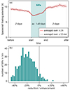 |
Fig. 17. Scaled superposed epoch analysis (top panel) and histogram of the reduction or enhancement during each event (bottom panel) of Wind’s floating potential during all SIRs that are associated with CIRs since 2005, in analogy to Fig. 12. The shaded red confidence band in the top panel corresponds to the standard deviation and a 1 V measurement uncertainty for individual measurements of the floating potential. The first fourteen SIRs of 2005 were not taken into account because no spacecraft floating potential data was available. |
However, Sect. 4.3.1 showed that the observed dust impacts are on average reduced during CIRs, contrary to the effect that is imposed by the change of the floating potential. While some CIRs appear to enhance the number of dust impact detections, it was shown in Sect. 4.3.1 that these CIRs cannot solely be responsible for the solar rotation signatures. Thus, the observed solar rotation signatures cannot be artificially created through CIR-induced changes of the floating potential but must come from a genuine reduction of dust impacts during CIRs. This indicates that the solar rotation signatures are not caused by periodic changes of the spacecraft’s floating potential but genuine patterns in the dust environment4.
4.5.2. Influence of the event selection by the fast time domain sampler
The data acquisition rate of the TDSF instrument is much higher than its data transmission rate. Therefore, the events measured by the TDSF are ranked by an algorithm, and only the highest-quality events are transmitted to Earth (Bougeret et al. 1995). Although the primary criterion by which the algorithm assesses an event’s quality is the event’s timestamp – a new event would replace the oldest event in the buffer – there were times when instead the events’ signal amplitudes were used as the primary criterion (Goetz, K., priv. comm.).
Ordinarily, the signals of dust impacts have higher amplitudes than those of most plasma waves. However, upstream of an interplanetary shock, bursts of high-amplitude plasma waves can occur (Wilson et al. 2010). These signals could fill the TDSF buffer and essentially make the instrument insensitive to dust impacts. If this were to systematically happen during CIRs, an artificial reduction of dust impacts by CIRs would be observed, resulting in artificial solar rotation signatures.
However, interplanetary shocks only rarely fill the TDSF buffer with high-amplitude events. These bursts of high-amplitude plasma waves following a shock last only for a few minutes (Cohen et al. 2020), and the TDSF buffer has room for only about twenty events that are continuously written onto the spacecraft’s tape recorder (Goetz, K., priv. comm.). In contrast, the reduction of dust impact detections associated with CIRs is observed on timescales of one to two days (Sect. 4.3.1). It is unlikely that the day-long observed reduction of dust impacts could have been caused by a possible minutes-long insensitivity to dust impacts.
Furthermore, less than a third of all CIRs recorded by Jian et al. (2006) are associated with interplanetary shocks, whereas most CIR passages are associated with a reduction of dust impact detections (see Sect. 4.3.1); it is, thus, unlikely that the observed reductions of dust impacts are caused by an instrumental insensitivity to dust impacts upstream of interplanetary shocks. This indicates that it is unlikely that the solar rotation signatures are artificially caused by selection biases of the TDSF ranking algorithm, but that the solar rotation signatures are genuine patterns in the dust environment5.
5. Summary and conclusions
Signatures of the solar rotation were discovered in the observations of cosmic dust impacts on the Wind spacecraft. The time series of these dust impact data (Malaspina & Wilson 2016), measured by Wind’s plasma wave instrument, was investigated in detail. A frequency analysis of the daily number of dust impacts measured at L1 between 1 January 2005 and 31 August 2023 yielded the following conclusion (Sect. 4.1): Solar rotation signatures are evident in the dust impact data as spectral peaks at ∼27 d, 13.5 d, and 9d.
Further, we investigated whether these solar rotation signatures are evident in the interplanetary or the interstellar component of dust impacts measured on Wind. More ISD impacts were observed when the spacecraft moved against the ISD inflow direction (February to April) compared to when it moved with the ISD inflow direction (August to October). Seasonal variations of the measured IDP impacts were assumed to be negligible. The solar rotation signatures were found in spectra of the daily number of dust impacts for both orbital configurations but were considerably stronger when the spacecraft moved against the ISD inflow direction, that is, when more ISD impacts were measured (Sect. 4.2.1).
Measurable dust impacts from ISD occur more frequently during the focusing phase of the solar magnetic cycle compared to the defocusing phase of the solar magnetic cycle. The solar rotation signatures were found in spectra of the daily number of dust impacts during both the focusing phase and the defocusing phase of the solar magnetic cycle but were considerably stronger during the focusing phase, that is, when more ISD impacts were measured (Sect. 4.2.2). This yielded the following conclusion: The solar rotation signatures are not caused exclusively by IDPs but are, at least partially, caused by ISD.
It is known that Jovian and Saturnian dust streams are affected by CIRs (Hsu et al. 2010; Flandes et al. 2011), and we therefore hypothesised that CIRs cause the solar rotation signatures. For this reason, a superposed epoch analysis for all CIRs was performed, and we found that dust impact detections are, on average, reduced during CIRs compared to the preceding and following time intervals (Sect. 4.3.1). Additionally, case studies of time periods of particular rates of occurrence of CIRs were investigated. We found that during time periods of long-lasting CIRs, the solar rotation signatures are powerful and that during time periods where no CIRs were observed, the solar rotation signatures vanish (Sect. 4.3.2). A synthetic time series of dust impacts that are completely depleted during CIRs generated comparable spectra for these case studies (Sect. 4.3.3). This yielded the following conclusions: The solar rotation signatures are correlated with and most likely caused by CIRs, and the number of dust impact detections is, on average, reduced during CIRs compared to the preceding and following time periods.
A competing hypothesis for the origin of the solar rotation signatures lies in the sector structure of the IMF, which is known to affect Jovian and Saturnian dust streams (Hamilton & Burns 1993; Hsu et al. 2010). Therefore, case studies of time periods when the IMF sector structure was stable or chaotic were investigated. We found that the solar rotation signatures for spectra of the daily number of dust impacts are not correlated with the solar rotation signatures of the IMF polarity. Powerful solar rotation signatures were observed in the dust impacts even at times when the sector structure was chaotic, and weak solar rotation signatures were observed at times when the sector structure was stable (Sect. 4.4). This yielded the following conclusion: The IMF sector structure local to the spacecraft cannot be the sole cause of the solar rotation signatures.
Solar rotation signatures have also been observed in spectra of Wind’s floating potential (Wilson et al. 2023a). It is known that changes in the spacecraft’s floating potential affect the signal amplitudes of a dust impact measured by dipole antennas (Shen et al. 2023). Therefore, it may be possible that the solar rotation signatures in the dust impact spectra do not stem from a genuine modulation of dust impacts but are artificially induced by changing the instrument’s sensitivity to dust impacts whenever a CIR passes. However, passing CIRs enhance the instrument’s sensitivity to dust impacts, partially counteracting the observed reduction of dust impacts during CIRs instead of artificially inducing it (Sect. 4.5.1). Thus, we made the following conclusion: Periodic changes of the spacecraft’s floating potential alone are an unlikely explanation of the solar rotation signatures in the dust impact data.
A similarly artificial origin of the solar rotation signatures could come from the fact that the TDS becomes temporarily insensitive to dust impacts upstream of interplanetary shocks due to a selection bias by the instrument. Interplanetary shocks can be associated with CIRs (Jian et al. 2006) and can thus artificially cause the solar rotation signatures. However, the timescale on which the instrument would be biased is much shorter than the timescale of the observed reduction of dust impact measurements during CIRs. Furthermore, only a fraction of CIRs are associated with interplanetary shocks (see Sect. 4.5.2). This yielded the following conclusion: A selection bias of the instrument against dust impact signals upstream of interplanetary shocks is unlikely to be the cause of the solar rotation signatures in the dust impact data.
In total, solar rotation signatures were found in the frequency spectra of the daily number of dust impacts recorded by Wind at periods of ∼27 d and its harmonics. Known instrumental effects were ruled out as the possible origin of these signatures, indicating that the signatures are genuine features of the dust environment. The most likely cause of these signatures is CIRs that reduce the number of dust impact detections as they pass the spacecraft. The solar rotation signatures showcase the close link between heliospheric and dust sciences, highlighting the need for cooperation and utilising the synergies between the two (cf., e.g. Sterken et al. 2023).
The physical mechanism that causes the observed reduction of dust impacts during CIRs is not well understood. While it may be similar to the mechanisms proposed by Ragot & Kahler (2003) and Wagner & Wimmer-Schweingruber (2009) for CMEs, further modelling efforts are required to investigate this possibility.
In order to examine the influence of the solar rotation on dust in greater detail, it is essential to not only know the signal amplitude of a particle impact but to be able to infer the impact speed and impactor mass and size from it. Likewise, being able to constrain the direction from which an impacting dust particle comes would facilitate clearer distinctions between interstellar and interplanetary origins of the particles. This requires space-based missions with dedicated dust detectors. In the near future the Interstellar Mapping and Acceleration Probe at L1 will carry the Interstellar Dust Experiment; however, this dust detector infers the impact speed of a dust particle from orbital dynamics and from the particle’s composition and does not determine it from measurements (McComas et al. 2018). A complementary (large-area) “dust telescope” (i.e. a trajectory grid combined with a time of flight mass spectrometer) that can directly determine the impact speed would be essential to have, for example, on board the Lunar Gateway (Wozniakiewicz et al. 2021; Arnet 2023; Sterken et al., in prep.) or on board the proposed SunCHASER mission at L4 (Posner et al. 2021; Cho et al. 2023).
The ecliptic plane, in which Earth and the Wind spacecraft revolve around the Sun, is itself inclined by 7° with respect to the solar equatorial plane; therefore, the Parker spiral can have a minor z-component even within the ecliptic plane. This is ignored within this study.
WI_L3-DUSTIMPACT_WAVES on https://cdaweb.gsfc.nasa.gov
We note that the magnetic field of a CME is considerably stronger close to the Sun than at 1 AU (e.g. Patsourakos & Georgoulis 2016).
The dust impact data of the STEREO spacecraft were measured with monopole antennas, which are only weakly affected by changes to the spacecraft floating potential (Shen et al. 2023); thus, the presence of the solar rotation signatures in the STEREO data by Chadda et al. (in prep.) corroborate our interpretation as genuine patterns in the dust.
Unlike the TDSF of Wind/WAVES, the dust impact data measured with S/WAVES onboard the STEREO spacecraft is not affected by this ranking algorithm’s selection issue, reaffirming that the solar rotation signatures are not caused by external influences but are genuine features of the dust environment.
Acknowledgments
We would like to thank the anonymous referee for excellent and thought-provoking comments, and Keith Goetz, Ming-Hsueh “Mitchell” Shen, O. Chris St. Cyr, Felix Dannert, Markus Bonse, Thomas Birbacher, Ingo Waldmann, and Kai Hou “Gordon” Yip for their suggestions and advice. V. J. Sterken, S. Hunziker, L. R. Baalmann, and A. Péronne received funding from the European Union’s Horizon 2020 research and innovation programme under grant agreement N° 851544 – ASTRODUST. S. Chadda and D. M. Malaspina acknowledge support from STEM Routes Uplift program (Packard Foundation 2021-72553), the Undergraduate Research Opportunities Program (UROP) at the University of Colorado, Boulder, NASA grant #80NSSC23K0286, and NASA grant #80NSSC22K0753. This work makes use of the Julia programming language, v1.10.2 (Bezanson et al. 2017), and its packages LsqFit.jl, Plots.jl (Breloff 2023), and SPICE.jl (Acton 1996). Author contributions: L.R.B. curated the data, performed the data analyses, and wrote and revised the manuscript. S.H. performed a preliminary data analysis and discovered the solar rotation signatures. A.P. performed the superposed epoch analyses and supplementary data analyses (cf. Péronne et al., in prep.) and revised the manuscript. J.W.K. devised the frequency analysis method and supported the data analyses; J.W.K. and K.-H.G. advised on the data analyses and the physical interpretation of their results, and revised the manuscript. D.M.M. and L.B.W.III acquired and provided the data and revised the manuscript; D.M.M. advised on the physical interpretation, and L.B.W.III advised on the instrumentation. C.S. performed a preliminary data analysis. S.C. enabled comparisons to spectra of the STEREO data (Chadda et al., in prep.). V.J.S. initiated and supervised the project, contributed to the original discovery, advised on the data analyses and the physical interpretation of their results, revised the manuscript, and acquired funding.
References
- Acton, C. H. 1996, Planet. Space Sci., 44, 65 [Google Scholar]
- Altobelli, N. 2004, Ph.D. Thesis, Ruprecht-Karls University of Heidelberg, Germany [Google Scholar]
- Andersson, L., Weber, T. D., Malaspina, D., et al. 2015, Science, 350, 0398 [Google Scholar]
- Arnet, T. 2023, Dust Science from the Lunar Gateway (Switzerland: ETH Zürich) [Google Scholar]
- Aubier, M. G., Meyer-Vernet, N., & Pedersen, B. M. 1983, Geophys. Res. Lett., 10, 5 [NASA ADS] [CrossRef] [Google Scholar]
- Auer, S. 2001, Interplanetary Dust (Berlin, Heidelberg: Springer), 385 [CrossRef] [Google Scholar]
- Balogh, A., Marsden, R. G., & Smith, E. J. 2001, The Heliosphere Near Solar Minimum. The Ulysses Perspective (London: Springer) [Google Scholar]
- Bezanson, J., Edelman, A., Karpinski, S., & Shah, V. B. 2017, SIAM Rev., 59, 65 [Google Scholar]
- Bougeret, J. L., Kaiser, M. L., Kellogg, P. J., et al. 1995, Space Sci. Rev., 71, 231 [CrossRef] [Google Scholar]
- Breloff, T. 2023, https://doi.org/10.5281/zenodo.7844522 [Google Scholar]
- Brownlee, D. E. 1985, Annu. Rev. Earth Planet. Sci., 13, 147 [CrossRef] [Google Scholar]
- Chen, C. H. K., Howes, G. G., Bonnell, J. W., et al. 2013, AIP Conf. Ser., 1539, 143 [NASA ADS] [Google Scholar]
- Cho, K.-S., Hwang, J., Han, J.-Y., et al. 2023, J. Korean Astron. Soc., 56, 263 [NASA ADS] [Google Scholar]
- Chree, C. 1913, Phil. Trans. R. Soc. A, 212, 75 [Google Scholar]
- Cohen, Z. A., Cattell, C. A., Breneman, A. W., et al. 2020, ApJ, 904, 174 [NASA ADS] [CrossRef] [Google Scholar]
- Collette, A., Grün, E., Malaspina, D., & Sternovsky, Z. 2014, J. Geophys. Res. Space Phys., 119, 6019 [NASA ADS] [CrossRef] [Google Scholar]
- Cumming, A., Marcy, G. W., & Butler, R. P. 1999, ApJ, 526, 890 [Google Scholar]
- Czechowski, A., & Mann, I. 2010, ApJ, 714, 89 [Google Scholar]
- Dietzel, H., Eichhorn, G., Fechtig, H., et al. 1973, J. Phys. E: Sci. Instrum., 6, 209 [NASA ADS] [CrossRef] [Google Scholar]
- Draine, B. T., & Lee, H. M. 1984, ApJ, 285, 89 [NASA ADS] [CrossRef] [Google Scholar]
- Dumbović, M., Vršnak, B., Temmer, M., Heber, B., & Kühl, P. 2022, A&A, 658, A187 [NASA ADS] [CrossRef] [EDP Sciences] [Google Scholar]
- Ferraz-Mello, S. 1981, AJ, 86, 619 [NASA ADS] [CrossRef] [Google Scholar]
- Flandes, A., Krüger, H., Hamilton, D. P., et al. 2011, Planet. Space Sci., 59, 1455 [NASA ADS] [CrossRef] [Google Scholar]
- Foster, G. 1995, AJ, 109, 1889 [CrossRef] [Google Scholar]
- Foster, G. 1996, AJ, 112, 1709 [NASA ADS] [CrossRef] [Google Scholar]
- Frisch, P. C., Dorschner, J. M., Geiss, J., et al. 1999, ApJ, 525, 492 [NASA ADS] [CrossRef] [Google Scholar]
- Fröhlich, C., & Lean, J. 1998, Geophys. Res. Lett., 25, 4377 [CrossRef] [Google Scholar]
- Garrett, H. B. 1981, Rev. Geophys., 19, 577 [CrossRef] [Google Scholar]
- Geyer, P., Temmer, M., Guo, J., & Heinemann, S. G. 2021, A&A, 649, A80 [NASA ADS] [CrossRef] [EDP Sciences] [Google Scholar]
- Gosling, J. T., & Pizzo, V. J. 1999, Space Sci. Rev., 89, 21 [NASA ADS] [CrossRef] [Google Scholar]
- Grün, E., Zook, H. A., Fechtig, H., & Giese, R. H. 1985, Icarus, 62, 244 [NASA ADS] [CrossRef] [Google Scholar]
- Grün, E., Zook, H. A., Baguhl, M., et al. 1993, Nature, 362, 428 [Google Scholar]
- Grün, E., Gustafson, B., Mann, I., et al. 1994, A&A, 286, 915 [Google Scholar]
- Grün, E., Gustafson, B. A. S., Dermott, S., & Fechtig, H. 2001, Interplanetary Dust (Berlin, Heidelberg: Springer) [CrossRef] [Google Scholar]
- Gurnett, D. A., Grün, E., Gallagher, D., Kurth, W. S., & Scarf, F. L. 1983, Icarus, 53, 236 [NASA ADS] [CrossRef] [Google Scholar]
- Gurnett, D. A., Averkamp, T. F., Scarf, F. L., & Grün, E. 1986, Geophys. Res. Lett., 13, 291 [NASA ADS] [CrossRef] [Google Scholar]
- Gustafson, B. A. S. 1994, Annu. Rev. Earth Planet. Sci., 22, 553 [CrossRef] [Google Scholar]
- Gustafson, B. A. S., & Misconi, N. Y. 1979, Nature, 282, 276 [NASA ADS] [CrossRef] [Google Scholar]
- Hajra, R., & Sunny, J. V. 2022, Sol. Phys., 297, 30 [NASA ADS] [CrossRef] [Google Scholar]
- Hamilton, D. P., & Burns, J. A. 1993, Nature, 364, 695 [NASA ADS] [CrossRef] [Google Scholar]
- Hervig, M. E., Malaspina, D., Sterken, V., et al. 2022, J. Geophys. Res. Space Phys., 127, e2022JA030749 [NASA ADS] [CrossRef] [Google Scholar]
- Hsu, H.-W., Kempf, S., & Jackman, C. M. 2010, Icarus, 206, 653 [NASA ADS] [CrossRef] [Google Scholar]
- Hsu, H. W., Postberg, F., Kempf, S., et al. 2011, J. Geophys. Res. Space Phys., 116, A09215 [NASA ADS] [Google Scholar]
- Jian, L. 2021, Stream Interaction Regions (SIRs) from Wind and ACE Data during 1995 – 2009, https://izw1.caltech.edu/ACE/ASC/DATA/level3/SIR_List_1995_2009_Jian.pdf [Google Scholar]
- Jian, L., Russell, C. T., Luhmann, J. G., & Skoug, R. M. 2006, Sol. Phys., 239, 337 [NASA ADS] [CrossRef] [Google Scholar]
- Jokipii, J. R., & Thomas, B. 1981, ApJ, 243, 1115 [NASA ADS] [CrossRef] [Google Scholar]
- Kellogg, P. J., Goetz, K., & Monson, S. J. 2016, J. Geophys. Res. Space Phys., 121, 966 [NASA ADS] [CrossRef] [Google Scholar]
- Kellogg, P. J., Goetz, K., & Monson, S. J. 2018, J. Geophys. Res. Space Phys., 123, 7211 [NASA ADS] [CrossRef] [Google Scholar]
- Kimura, H., & Mann, I. 1999, in Meteroids 1998, eds. W. J. Baggaley, & V. Porubcan, 283 [Google Scholar]
- Kirchner, J. W., & Neal, C. 2013, Proc. Natl. Acad. Sci., 110, 12213 [CrossRef] [Google Scholar]
- Krüger, H., Strub, P., Grün, E., & Sterken, V. J. 2015, ApJ, 812, 139 [CrossRef] [Google Scholar]
- Krüger, H., Strub, P., Altobelli, N., et al. 2019, A&A, 626, A37 [NASA ADS] [CrossRef] [EDP Sciences] [Google Scholar]
- Kurth, W. S., Averkamp, T. F., Gurnett, D. A., & Wang, Z. 2006, Planet. Space Sci., 54, 988 [NASA ADS] [CrossRef] [Google Scholar]
- Landgraf, M. 1998, Ph.D. Thesis, Ruprecht-Karls University of Heidelberg, Germany [Google Scholar]
- Landgraf, M. 2000, J. Geophys. Res., 105, 10303 [NASA ADS] [CrossRef] [Google Scholar]
- Leinert, C., Link, H., Pitz, E., & Giese, R. H. 1976, A&A, 47, 221 [NASA ADS] [Google Scholar]
- Liou, K., & Wu, C.-C. 2021, ApJ, 920, 39 [NASA ADS] [CrossRef] [Google Scholar]
- Lomb, N. R. 1976, Ap&SS, 39, 447 [Google Scholar]
- Ma, Q., Matthews, L. S., Land, V., & Hyde, T. W. 2013, ApJ, 763, 77 [NASA ADS] [CrossRef] [Google Scholar]
- Malaspina, D. M., Horányi, M., Zaslavsky, A., et al. 2014, Geophys. Res. Lett., 41, 266 [NASA ADS] [CrossRef] [Google Scholar]
- Malaspina, D. M., & Wilson, L. B., III 2016, J. Geophys. Res. Space Phys., 121, 9369 [CrossRef] [Google Scholar]
- Mathis, J. S., Rumpl, W., & Nordsieck, K. H. 1977, ApJ, 217, 425 [Google Scholar]
- McComas, D. J., Christian, E. R., Schwadron, N. A., et al. 2018, Space Sci. Rev., 214, 116 [CrossRef] [Google Scholar]
- Meyer-Vernet, N., Maksimovic, M., Czechowski, A., et al. 2009, Sol. Phys., 256, 463 [NASA ADS] [CrossRef] [Google Scholar]
- Moorhead, A. V. 2021, Icarus, 354, 113949 [NASA ADS] [CrossRef] [Google Scholar]
- Morfill, G. E., & Grün, E. 1979, Planet. Space Sci., 27, 1283 [NASA ADS] [CrossRef] [Google Scholar]
- Mukai, T. 1981, A&A, 99, 1 [NASA ADS] [Google Scholar]
- O’Brien, L., Juhász, A., Sternovsky, Z., & Horányi, M. 2018, Planet. Space Sci., 156, 7 [CrossRef] [Google Scholar]
- Owens, M. J., & Forsyth, R. J. 2013, Liv. Rev. Sol. Phys., 10, 5 [Google Scholar]
- Page, B., Bale, S. D., Bonnell, J. W., et al. 2020, ApJS, 246, 51 [Google Scholar]
- Parker, E. N. 1958, ApJ, 128, 664 [Google Scholar]
- Patsourakos, S., & Georgoulis, M. K. 2016, A&A, 595, A121 [NASA ADS] [CrossRef] [EDP Sciences] [Google Scholar]
- Posner, A., Arge, C. N., Staub, J., et al. 2021, Space Weather, 19, e02777 [NASA ADS] [CrossRef] [Google Scholar]
- Ragot, B. R., & Kahler, S. W. 2003, ApJ, 594, 1049 [NASA ADS] [CrossRef] [Google Scholar]
- Richardson, I. G. 2018, Liv. Rev. Sol. Phys., 15, 1 [Google Scholar]
- Robertson, H. P. 1937, MNRAS, 97, 423 [NASA ADS] [Google Scholar]
- Scargle, J. D. 1982, ApJ, 263, 835 [Google Scholar]
- Shen, M. M., Sternovsky, Z., Horányi, M., Hsu, H.-W., & Malaspina, D. M. 2021, J. Geophys. Res. Space Phys., 126, e28965 [NASA ADS] [Google Scholar]
- Shen, M. M., Sternovsky, Z., & Malaspina, D. M. 2023, J. Geophys. Res. Space Phys., 128, e2022JA030981 [CrossRef] [Google Scholar]
- Slavin, J. D., Frisch, P. C., Müller, H.-R., et al. 2012, ApJ, 760, 46 [NASA ADS] [CrossRef] [Google Scholar]
- St. Cyr, O. C., Wilson, L. B., Rockcliffe, K., et al. 2017, AGU Fall Meeting Abstracts, 2017, SH23D–2682 [Google Scholar]
- Stenborg, G., Paouris, E., Howard, R. A., Vourlidas, A., & Hess, P. 2023, ApJ, 949, 61 [NASA ADS] [CrossRef] [Google Scholar]
- Sterken, V. J., Altobelli, N., Kempf, S., et al. 2012, A&A, 538, A102 [NASA ADS] [CrossRef] [EDP Sciences] [Google Scholar]
- Sterken, V. J., Altobelli, N., Kempf, S., et al. 2013, A&A, 552, A130 [NASA ADS] [CrossRef] [EDP Sciences] [Google Scholar]
- Sterken, V. J., Strub, P., Krüger, H., von Steiger, R., & Frisch, P. 2015, ApJ, 812, 141 [NASA ADS] [CrossRef] [Google Scholar]
- Sterken, V. J., Westphal, A. J., Altobelli, N., Malaspina, D. M., & Postberg, F. 2019, Space Sci. Rev., 215, 43 [NASA ADS] [CrossRef] [Google Scholar]
- Sterken, V. J., Baalmann, L. R., Draine, B. T., et al. 2022, Space Sci. Rev., 218, 71 [CrossRef] [Google Scholar]
- Sterken, V. J., Hunziker, S., Dialynas, K., et al. 2023, RAS Tech. Instrum., 2, 532 [NASA ADS] [CrossRef] [Google Scholar]
- Strub, P., Krüger, H., & Sterken, V. J. 2015, ApJ, 812, 140 [NASA ADS] [CrossRef] [Google Scholar]
- Strub, P., Sterken, V. J., Soja, R., et al. 2019, A&A, 621, A54 [NASA ADS] [CrossRef] [EDP Sciences] [Google Scholar]
- Svalgaard, L. 2023a, IMF Sector Boundaries, https://svalgaard.leif.org/research/sblist.txt [Google Scholar]
- Svalgaard, L. 2023b, IMF Sector Structure Polarity, https://svalgaard.leif.org/research/spolar.txt [Google Scholar]
- Swaczyna, P., Bzowski, M., Kubiak, M. A., et al. 2018, ApJ, 854, 119 [NASA ADS] [CrossRef] [Google Scholar]
- Tsurutani, B. T., Clay, D. R., Zhang, L. D., et al. 2004, Icarus, 167, 89 [NASA ADS] [CrossRef] [Google Scholar]
- VanderPlas, J. T. 2018, ApJS, 236, 16 [Google Scholar]
- Vaverka, J., Pellinen-Wannberg, A., Kero, J., et al. 2017, J. Geophys. Res. Space Phys., 122, 6485 [CrossRef] [Google Scholar]
- Vaverka, J., Nakamura, T., Kero, J., et al. 2018, J. Geophys. Res. Space Phys., 123, 6119 [NASA ADS] [CrossRef] [Google Scholar]
- Wagner, M., & Wimmer-Schweingruber, R. F. 2009, A&A, 507, L41 [NASA ADS] [CrossRef] [EDP Sciences] [Google Scholar]
- Wang, X., Malaspina, D. M., Ergun, R. E., & Horányi, M. 2014, J. Geophys. Res. Space Phys., 119, 1094 [NASA ADS] [CrossRef] [Google Scholar]
- Watson, W. D. 1973, J. Opt. Soc. Am. (1917–1983), 63, 164 [CrossRef] [Google Scholar]
- Wehry, A. 2002, Ph.D. Thesis, Ruprecht-Karls University of Heidelberg, Germany [Google Scholar]
- Wehry, A., & Mann, I. 1999, A&A, 341, 296 [NASA ADS] [Google Scholar]
- Wehry, A., Krüger, H., & Grün, E. 2004, A&A, 419, 1169 [NASA ADS] [CrossRef] [EDP Sciences] [Google Scholar]
- Wilson, L. B., Cattell, C. A., Kellogg, P. J., et al. 2010, J. Geophys. Res. Space Phys., 115, A12104 [NASA ADS] [Google Scholar]
- Wilson, L. B., III, Brosius, A. L., Gopalswamy, N., et al. 2021, Rev. Geophys., 59, e2020RG000714 [NASA ADS] [CrossRef] [Google Scholar]
- Wilson, L. B., III, Salem, C. S., & Bonnell, J. W. 2023a, ApJS, 269, 52 [NASA ADS] [CrossRef] [Google Scholar]
- Wilson, L. B., III, Salem, C. S., & Bonnell, J. W. 2023b, https://doi.org/10.5281/zenodo.8364797 [Google Scholar]
- Wozniakiewicz, P. J., Bridges, J., Burchell, M. J., et al. 2021, Adv. Space Res., 68, 85 [NASA ADS] [CrossRef] [Google Scholar]
- Zaslavsky, A., Meyer-Vernet, N., Mann, I., et al. 2012, J. Geophys. Res. Space Phys., 117, A05102 [NASA ADS] [CrossRef] [Google Scholar]
- Zaslavsky, A., Mann, I., Soucek, J., et al. 2021, A&A, 656, A30 [NASA ADS] [CrossRef] [EDP Sciences] [Google Scholar]
- Zook, H. A., & Berg, O. E. 1975, Planet. Space Sci., 23, 183 [Google Scholar]
- Zook, H. A., Grun, E., Baguhl, M., et al. 1996, Science, 274, 1501 [NASA ADS] [CrossRef] [Google Scholar]
Appendix A: Data reduction
The daily number of dust impacts contained in the dataset is depicted in Fig. A.1 without applying the corrections of Sect. 3.3; for convenience, a moving average with a centred window of 91 d, corresponding to roughly a quarter of the spacecraft’s orbital period, is graphed as well. Many external influences affected the recordings of dust impacts on Wind in its almost thirty years of service (Appendix A.1). These influences are not taken into account in Fig. A.1, but the times when they occurred are marked by vertical lines and shaded areas in the figure.
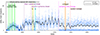 |
Fig. A.1. Unprocessed data presented as the daily number of impacts. Each pale blue disc corresponds to the number of impacts during one calendar day; a moving average within a centred window of 91 d is given by the black line. The many external influences (see Appendix A.1), marked by vertical lines and shaded areas, are not taken into account in this representation of the unprocessed data. |
These influences include the times when a twice-as-high data transfer rate was used before 1998, the two incidents on 3 August 2000 and 25 September 2002 in which the x-antenna was shortened, the change of the sampling rate on 1 April 2011, and the two time intervals when no dust impacts could be recorded due to an incorrect trigger setting in 2013 and due to a system outage in late 2014. For convenience, the times when Wind briefly visited L1 in 2003 and L2 in 2003-2004 are indicated as well. Before the spacecraft began permanently orbiting L1 in 2004-2005, the number of daily impacts appears to be strongly influenced by the distance to Earth (Appendix A.5); this time interval is marked as well.
These external influences must be taken into account when analysing the daily number of dust impacts. Changes to the instrument that influenced the general availability of the data, such as the use of the high data transfer rate before 1998, can be approximately corrected for by normalising the daily number of dust impacts by the total number of events the TDSF registered (Appendix A.3). However, this introduces biases and should only be used if no other means of correction are available.
Another external influence that must be taken into account is the change of the sampling rate in 1 April 2011 (Appendix A.4), which is especially evident in Fig. A.1: since April 2011, the moving average of the daily number of dust impacts is systematically shifted to lower values, and days with no impacts occur frequently and periodically.
Some influences cannot be corrected for directly, such as the distance dependence of the daily number of dust impacts (Appendix A.5) or the antenna cuts. These must be taken into account otherwise, for example by removing the affected data.
A.1. Summary of known influences
To summarise, the dust impact dataset is externally influenced by instrumental effects. Chronologically ordered, the known influences are:
-
The quality of a TDSF event is assessed by a ranking algorithm, referred to as a neural network. If the memory buffer of the time domain sampler (TDS) subsystem is full, the lowest-quality event is discarded. The best-quality event from the TDS memory buffer is written onto the spacecraft’s tape recorder and later transmitted to Earth whenever the WAVES telemetry stream has sufficient idle capacity (Bougeret et al. 1995). The effect of a possible selection bias of the ranking algorithm is investigated in Sect. 4.5.2.
-
The TDS subsystem has the lowest telemetry priority of all WAVES subsystems (Goetz, K., priv. comm.). If other subsystems deliver more data, less telemetry bandwidth is available for the TDS.
-
The sampling rate of the TDSF is changed from 120 kS/s to a lower setting of 30 kS/s for one hour at 21:00 Terrestrial Time (TT) every two days. During this time, no dust impacts can be measured.
-
Until the end of 1998, a twice-as-high telemetry acquisition bit rate was used whenever the spacecraft was close to Earth (Appendix A.3). During these time periods, more detections of dust impacts could be sent to Earth.
-
For unknown reasons the TDSF measured a low number of daily events from 1998 to 2000 (Appendix A.3). This also decreased the number of observed dust impacts.
-
The X+-antenna arm was cut on 3 August 2000 and on 25 September 2002. This has altered the amplitude distribution measured by the x-dipole (Kellogg et al. 2016); see Appendix A.2.
-
For unknown reasons the dust impacts are correlated with the distance to Earth until the spacecraft began continuously orbiting L1 in 2005 (Appendix A.5).
-
Since 1 April 2011 the TDSF sampling rate is periodically changed from 120 kS/s to 30 kS/s. For 45 h 36 min out of every six days no dust impacts can be measured (cf. Appendix A.4).
-
From 1 February 2013 to 8 July 2013 the z-dipole was used as a trigger for the TDS. Only spurious events were measured during this time.
-
From 25 October 2014 to 24 November 2014 the Wind spacecraft was unable to measure any dust impacts due to a double single event upset, likely caused by a cosmic ray particle impact.
For long-term analyses it is expedient to only use the dataset since 1 January 2005, when Wind continuously orbited L1. The periodically occurring measurement gaps and the general measurement gaps of 2013 and 2014 must be accounted for. Only dust impacts with morphological types A and B were taken into account (see Sect. 3.3; Appendix B.6). When investigating the signal amplitudes generated by the dust impacts, only the signal amplitudes measured by the y-antenna (Channel 2) should be used (see Appendix A.2).
A.2. Removal of events
The dataset contains a total of 141 438 dust impacts. According to the location flag given in the database, 843 (≈0.60%) were measured when Wind was located in the Earth’s magnetosphere, and one was measured in the lunar wake; 1417 (≈1.00%) entries are assigned the location flag “N/A”. These entries were removed from the dataset, resulting in 139 177 valid entries, 98.4% of the whole dataset. Reducing the dataset to the time period since 2005 further decreased the total number of impacts to 95 895, and taking into account only impact signals with morphological types A and B yielded a total of only 83 203 dust impacts.
From 1 February 2013 to 8 July 2013, the z-antenna was used as the trigger for TDSF recordings for 157 d (Malaspina & Wilson 2016). 30 spurious events were measured during this period; these events were removed from the dataset.
Figure A.2 displays the amplitude distributions for both the x- and the y-antenna before the first antenna break and after the second break of the x-antenna. After the x-antenna was broken, its amplitude distribution was affected by the asymmetry of its two arms. For example, the x-antenna measured many more impacts with positive amplitudes than with negative amplitudes. For this reason, only the amplitude values recorded by the y-antenna were used (see Sect. 3.4.2). This reduced the number of available dust impact signals to 58 053, about two thirds of all impacts of morphological types A and B.
If the signal amplitudes are not of interest, as was the case for the frequency analyses in Sect. 4, all 83 203 dust impacts with morphological types A and B can be taken into account. Because dust impacts signals of types C and D are rare compared to those of types A and B, the power spectra of dust impacts with only morphological types A and B do not systematically differ from the spectra of dust impacts with all morphological types, except that the slightly reduced number of dust impacts results in slightly lower periodogram amplitudes. Dust impacts with morphological types C and D are briefly investigated in Appendix B.6.
A.3. Normalisation of the dust impact rate by the total event rate measured by the fast time domain sampler
The daily number of dust impacts in Fig. A.1 shows many unexpected features. One of these is the bell-shaped feature spanning the time interval from 1995 to 1999, during which the data transfer rate repeatedly changed: until the end of 1998, a twice-as-high telemetry acquisition bit rate was in use whenever the spacecraft was closer than ∼100 R⊗ ≈ 6.4 × 10⁵ km to Earth; after 1998 this mode was no longer used due to concerns regarding the tape recorders on Wind (Goetz, K., priv. comm.). Of all WAVES subsystems the TDS benefited most from the twice-as-high bit rate; it was allocated three times as much bandwidth compared to the low bit rate (Bougeret et al. 1995). This strongly affects the rate of measured TDSF events. Another unexpected feature in Fig. A.1 is the low number of dust impacts around the year 1999, which is caused by unspecified instrumental effects.
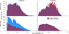 |
Fig. A.2. Amplitude distribution of type A and B dust impact signals before the first antenna break on 8 August 2000 (top row) and after the second antenna break on 9 September 2002 (bottom row) for the x-antenna (Channel 1; left column) and for the y-antenna (Channel 2; right column), separated into positive (blue) and negative (red) amplitudes. |
These two features do not reflect physical changes in the dust environment but were caused by changes of the instrumentation. It can therefore be expedient to normalise the daily number of dust impacts by the daily number of all TDSF events, which is available in the dust impact dataset (Malaspina & Wilson 2016) and plotted in Fig. A.3.
These data show the effect of the high data transfer rate until 1998 as the globally highest peaks, and that the overall rate of TDSF events between 1998 and 2000 is much lower compared to other time intervals. It is, at this point, not known why the daily number of TDSF events is much lower from 1998 to 2000 compared to other time intervals. The sudden increase in 2000 from, on average, well below 100 events per day to almost 200 events per day aligns with the shutdown of the Transient Gamma-Ray Spectrometer (TGRS) in January 2000 (Wilson et al. 2021); however, the WAVES instrument was always allocated the same portion of the bandwidth.
The normalisation of the dust impact rate by the TDSF event rate does not correct for all external influences and introduces biases on the dust impact rate. This normalisation is only appropriate under the assumption that the TDSF rate is a useful measure for how many dust impacts could have been recorded on a given day. For example, when the twice-as-high telemetry rate was in use, the TDS instrument was allocated three times as much bandwidth. The normalisation implies that this telemetry rate would similarly allow three times as many dust impacts to be transmitted to Earth.
This is, however, not necessarily true. Because the TDSF data acquisition rate of more than 2 Mb/s is orders of magnitude higher than the telemetry rate of the WAVES instrument of 944 b/s, the events to be transmitted are selected by a ranking algorithm, referred to as a neural network (Bougeret et al. 1995). There is no fundamental reason to assume that this ranking algorithm is unbiased with respect to dust impact signals compared to other plasma wave signals. The effect of a selection bias against dust impact signals when high-amplitude plasma waves are registered upstream of interplanetary shocks is investigated in Sect. 4.5.2.
Another bias is evident in the data: the daily number of TDSF events shows two distinct levels in Fig. A.3: one slightly below 200 events per day, and one at approximately 250 events per day. The TDSF rate varies between these two levels regularly with a period of 6 d for unknown reasons. Performing spectral analysis on the daily number of TDSF events reveals this periodicity as the most powerful peak of the periodogram. For the daily number of dust impacts before April 2011, spectral analysis finds only a weak 6 d-peak; after April 2011 this spectral peak becomes more powerful due to the periodic sampling rate changes.
If the 6 d-periodicity of the TDSF events had directly caused a similarly powerful 6 d-periodicity of the dust impact data, normalising the daily number of dust impacts by the daily number of TDSF events should decrease the periodogram amplitude of this peak. However, performing this normalisation artificially increases the power of the 6 d-peak in the dust data, indicating that normalising the dust impact data by the TDSF data artificially induces instrumental biases.
To summarise, normalising the dust impact data by the TDSF data has the advantage of accounting for the instrumental effects that predominantly occurred before the year 2000; its disadvantage is that the normalisation induces patterns of the TDSF data that may not be present in the dust impact data, such as a powerful 6 d-periodicity. Therefore, it is essential to normalise the dust impact data by the TDSF data when investigating the time period before 2000, especially if short-term variations on timescales similar to 6 d are not of particular interest. This is the case in Appendix A.5, which investigates the time period before Wind reached L1 in 2004.
When short-term variations are of interest, especially if only the dust impacts observed at L1 post-2004 are investigated, the main advantage of the normalisation no longer applies and its disadvantage becomes relevant. Thus, with the exception of Appendix A.5, the dust impact data were not normalised by the TDSF data within the scope of this study.
A.4. Correction for the sampling rate change in April 2011
Since April 2011, due to a periodic change of the sampling rate, the TDSF is insensitive to dust impacts for 45 h 36 min = 1.9 d out of every six days (see Sect. 3.1). Therefore, when investigating long-term patterns of the daily number of dust impacts, these periodic measurement gaps must be accounted for. When calculating the daily number of dust impacts it is expedient to delete the two days during which the 1.9 d-long gap occurred, even though this discards an additional 2 h 24 min of dust impacts every 6 d.
The daily number of TDSF events is also affected by the sampling rate change, but its influence is not so easily quantified. In analogy to the treatment of the dust impact dataset, it is expedient to delete the same two full days of TDSF data whenever the sampling rate was changed.
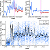 |
Fig. A.4. Daily number of dust impacts and TDSF events, corrected for the sampling rate change in April 2004. Top panel: Daily number of dust impacts (left) and daily number of TDSF events (right) as moving averages with centred windows of 91 d. The red curves depict the “raw” data – same as in Figs. A.1 and A.3 but additionally taking into account the data gaps of 2013 and 2014, which are marked by grey bars. The blue curves depict the same data but corrected for the change of the sampling rate in April 2011, which is marked by a vertical dotted magenta line. Bottom panel: Daily number of dust impacts normalised by the daily number of TDSF events, graphed for each individual day (blue discs) and as a moving average with a centred window of 91 d (black curve). The data have been corrected for the sampling rate change and the data gaps. |
This is depicted in Fig. A.4, where the top left panel shows a 91 d centred moving average of the daily number of dust impacts before and after correcting for the sampling rate change by deleting two full days of data; the top right panel shows the same for the daily number of TDSF events. As the figure indicates, the corrected data shows a similar pattern post-2011 and pre-2011: for the daily number of dust impacts, the yearly minimum before 2011 ranged around 15 impacts per day; for the uncorrected (“raw”) data, it dropped to about 10 impacts per day, whereas for the corrected data the minima remain at about 15 impacts per day. Similarly, the TDSF rate before April 2011 stands at about 180 events per day; the uncorrected (“raw”) data dropped to about 150 events per day after April 2011, and the corrected data again match the pre-2011 level.
The bottom panel of Fig. A.4 depicts the TDSF-normalised daily number of dust impacts. The figure shows that the bell-shaped feature before 1998 now resembles the yearly modulation expected from Wind’s orbit around the Sun. The high values in 1998 and 1999 are most likely unphysical; during this time, the TDSF rate was unusually low for unknown reasons. The unusual feature in 2003-2004, which is present in both the dust impacts, the TDSF events, and the normalised dust impacts, is assumed to be unphysical; its origin is unknown. After 2005, the normalised dust impact rate is overall similar to the unnormalised dust impact rate because the TDSF rate remains, on average, reasonably constant. The time interval before 2005, when Wind’s orbit frequently changed, is investigated in Appendix A.5.
A.5. Distance dependence pre 2005
Figure A.5 shows both the normalised daily number of dust impacts and the spacecraft’s distance to Earth in the time interval of 1995 to 2005. During this time, Wind frequently changed orbits (cf. Wilson et al. 2021, Fig. 1). For convenience, the normalised number of dust impacts has been graphed in Fig. A.5 as a centred moving average with a window width of 45 d. As the figure shows, the two displayed curves appear to be correlated with each other; a longer distance to Earth coincides with a higher normalised number of dust impacts. This correlation is not perfect: in the time interval between 1998 and 2000, where fewer TDSF events were measured, the normalised number of dust impacts is much higher than for other time intervals, excepting the brief visit to L1 in 2003; and during the visit to L2 in 2003-2004, no such correlation between the normalised number of dust impacts and the distance to Earth seems apparent. However, over the entire time interval between 1995 to 2005, the two curves are correlated; Pearson’s correlation coefficient gives a value of 0.5 compared to −0.03 for the time period between 2005 and 2021, when Wind continuously orbited L1.
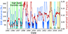 |
Fig. A.5. Distance of the spacecraft to Earth (smooth blue curve; left vertical axis) and normalised daily dust impacts (jagged red curve; right vertical axis) with a centred moving average of 45 d. The time intervals when the high data transfer rate was in use and the times spent at the Lagrange points are indicated by shaded areas. The distance to Earth is given in Earth radii, 1 Re ≈ 6378 km. |
This apparent distance dependence of the rate of dust impacts on the spacecraft is unexpected. Its cause is unknown and requires further investigation. To avoid unduly affecting the data analysis, all data before 2005 were excluded for the analyses performed in this work.
Appendix B: Details of the frequency analysis
The method for frequency analysis proposed by Kirchner & Neal (2013, Suppl. Mat.) resembles the Lomb-Scargle transform (Lomb 1976; Scargle 1982) with the time-shift factor, τ, modified to produce mutually orthogonal cosine and sine terms and thus eliminate the phase and amplitude artefacts of the Lomb-Scargle method; see Eqs. (S5-S9) of Kirchner & Neal (2013) for a formal description.
Within the scope of this publication, spectra were evaluated on a frequency grid that ranged from the fundamental frequency, fmin = 1/(tmax − tmin), where tmax − tmin is the total time interval covered by the dataset, to fmax = fNy = 0.5fS, where fNy is the Nyquist frequency of evenly sampled data, which is half the sampling frequency, fS. This grid was divided into n/2 equidistant points, where n is the number of data points. If the dataset contained no gaps, this frequency grid would reduce to the natural frequencies of the DFT. The frequency grid was oversampled by a factor of k, which increased the sampling density by that factor k.
As an example, the general dataset at L1 covers the time range from 7 January 2005 to 31 August 2023, which is a total time span of 6810 d. Thus, the fundamental frequency is fmin = 1/(6810 d). Because the time series of daily numbers of impacts are analysed, the sampling period is 1 d and, thus, the Nyquist frequency is fmax = 1/(2 d). If the dataset were to contain no gaps, i.e. if it were evenly sampled, the frequency grid would consist of n/2 = 3405 equidistant frequencies ranging from fmin = 1/(6810 d) to fmax = 1/(2 d).
However, in this dataset, only n = 5161 data points contain evaluable data and, thus, the frequency grid is coarser than the frequency grid of evenly sampled data. This is ameliorated by oversampling the frequency grid by a factor k, i.e. the frequency grid ranging from the same fmin to fmax is divided into nk/2 equidistant frequencies. Typical values are for k are k ∈ {2, 5, 10, 15, 20}, depending on the desired sampling density and computational cost. While oversampling doesn’t increase the resolution of the spectrum, i.e. neighbouring peaks cannot be resolved any better on an oversampled frequency grid, it does increase the precision of the frequency corresponding to a peak. For evenly sampled data, the method proposed by Kirchner & Neal (2013) perfectly reproduces the results of the DFT.
The spectra are given as periodograms; the periodogram amplitude is the squared amplitude of the fitted sinusoids, here in units of (amplitude)2 = (number of dust impacts per day)2. In the literature, spectra are also often given in terms of the power spectral density (PSD), which has the dimension (amplitude)2/frequency; here the frequency is measured in d−1. The periodogram amplitude can be converted to the PSD by multiplying with the total time interval covered by the data. The advantage of the periodogram compared to the PSD is that the periodogram amplitudes of peaks that correspond to periodic signals are independent from the length of the dataset; the broadband noise level decreases for longer datasets. Conversely, in a PSD the broadband noise level is independent of the length of the dataset, whereas the spectral power of peaks that correspond to periodic signals increase with the dataset length. In this work, spectra are represented by periodograms, facilitating a comparison of the peaks of periodic signals between data subsets of different lengths.
Before computing a spectrum, the data were linearly detrended by subtracting from the data a linear fit to the data. The linear fitting was performed by the LsqFit.jl6 package for the Julia programming language.
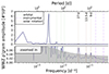 |
Fig. B.1. WWZ periodogram of the daily number of dust impacts recorded at L1, in analogy to Fig. 9. The bottom panel shows a zoomed-in view of the full spectrum, with the estimated 95% significance thresholds indicated by a grey shaded area. |
In addition to the phase and amplitude artefacts mentioned above, uneven sampling can also result in spectral aliasing, in which strong signals at one frequency appear as spurious signals at other frequencies. These aliases can be effectively suppressed using Kirchner and Neal’s variant of Foster’s Weighted Wavelet Z approach (WWZ; Foster 1996; Kirchner & Neal 2013). Figure B.1 shows this approach applied to the same data shown in Fig. 9. The solar rotation peaks at 27 d, 13.5 d, and 9 d are clearly visible in both Fig. B.1 and Fig. 9, indicating that they are not aliases generated by the uneven sampling of the time series. The much stronger peak at 6 d in Fig. 9, which arises as an alias of the 365 d-cycle, is suppressed below the 95% significance threshold in Fig. B.1.
B.1. Estimation of the 95% significance thresholds
The 95% significance thresholds of a periodogram were estimated through bootstrapping:
-
(1)
The non-NaN values of the underlying time series were reshuffled, i.e. randomly reordered. NaN values, i.e. known measurement gaps, were not affected by this reshuffling and remained at the same timestamps. The total sum of all values remained the same.
-
(2)
The periodogram of the reshuffled time series was calculated with the previously introduced methodology; the time series was linearly detrended beforehand. To decrease computational costs, the frequency grid was typically subsampled by a factor of k = 0.1.
-
(3)
This was repeated for a total of 5000 periodograms of randomly reshuffled time series.
-
(4)
For each frequency the 95% significance thresholds were estimated as the 95th percentile of the periodogram amplitudes of all 5000 periodograms.
Due to the measurement gaps, i.e. because the time series is not evenly sampled, the estimated 95% significance thresholds are not expected to be constant over all frequencies.
B.2. Effect of the 6 d-periodic gaps
Every six days, measured by the day-of-year of each year, a change of the instrument’s sampling rate made it impossible to detect impacts of dust particles for 45 h 36 min (Sect. 3.1). Because the daily number of dust impacts are analysed in this publication, this leads to two days of very few dust impacts every six days. To combat this, the entire two days were removed from the dataset, creating periodic gaps (Sect. A.4).
Periodic gaps do not, by themselves, create additional peaks in the power spectrum. However, where a sinusoid signal of frequency fsig will show a spectral peak at only fsig, the same signal with fgap-periodic gaps will show additional peaks. These stem from the convolution of the original signal with the receiver function, which is zero during gaps and one everywhere else. These peaks appear at frequencies |fsig, i ± fgap, j|, where i iterates over every genuine frequency of the signal, and j iterates over the relevant frequency and all harmonics of the receiver function.
Therefore, a spectrum of data with periodic gaps will be affected. In the case of fsig ≪ fgap these peaks will appear close to fgap; for example for the seasonal variability ( ) and
) and  , additional peaks appear at
  . For fsig ≲ fgap, these gaps are more easily confused with genuine periodicities; for example, for
  an additional peak would appear at
  .
.
This effect is one reason why peaks can appear at a period of 6 d and its 3 d-harmonic in the spectra, for example in Fig. 9. It can be suppressed by more elaborate methods such as the WWZ (see Fig. B.1). Another potential source of these spectral peaks could have been that the timing of the measurement gaps was misaligned with the removal of the data. This, however, could be disproved (see Fig. B.2).
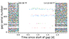 |
Fig. B.2. Superposed epoch analysis of all gaps stemming from the 6 d-periodic sampling rate change; serial number of the gaps versus time since the start of the two days of removed data. Each dot corresponds to one observed dust impact; each line of identically coloured dots corresponds to the same epoch, i.e. gap serial number. The vertical dashed black lines correspond to the reported timing of the sampling rate change. |
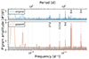 |
Fig. B.3. Periodogram of the daily number of dust impacts with morphological types A and B before April 2011, original data (blue curve, top panel) and data with artificially induced 6 d-periodic gaps (orange curve, bottom panel), evaluated at the DFT’s natural frequencies and oversampled by a factor of five. The two panels are scaled identically. Frequencies of interest are marked by vertical lines, as in Fig. 9. The estimated 95% significance thresholds are indicated by grey shaded areas. |
Figure B.2 shows a superposed epoch analysis (Chree 1913) of all gaps corresponding to the 6 d-periodic sampling rate changes. The sampling rate was reported to be reduced from  until
until  , which has been marked in the figure. While the start time of these sampling rate changes agrees with the observations, many dust impacts were already measured in the hour after 1 d + 21 : 00 TT = 1.875 d. Nevertheless, the interval of reduced sampling rate lies fully within the interval [0, 2] d that was removed from the dataset. The observational gaps are not misaligned with the data that was removed.
Some additional features remain in Fig. B.2: the two horizontal gaps around gap serial numbers 130 and 220 correspond to the long-term gaps of 2013 and 2014 (see Sect. A.2), respectively. For 13 gaps dust impacts were observed during the time where the detector was unable to detect dust impacts; the reason for this is unknown. The void that appears between ![Mathematical equation: $ [-0.125,-0.08\bar{3}]\,\mathrm{d} $](/articles/aa/full_html/2024/09/aa50069-24/aa50069-24-eq16.gif) , especially visible at high gap serial numbers, corresponds to a short-term sampling rate change that occurred every 2 d (see Appendix A.1).
, especially visible at high gap serial numbers, corresponds to a short-term sampling rate change that occurred every 2 d (see Appendix A.1).
The effect of the 6 d-periodic gaps on the generated spectra is displayed in Fig. B.3. For the data before the sampling rate was periodically changed in April 2011, artificial gaps following the same pattern at which the instrumental gaps occurred were induced on the originally continuous time series; the spectra for both the original and the gapped time series are shown in the figure.
The most obvious difference between the two spectra are the additional peaks close to 6 d and 3 d, which result from the convolution of the original time series with the receiver function, which is zero during gaps and one everywhere else. Some peaks of the original spectrum, such as the 9 d- and the 13.5 d-peaks, appear at the exact same period but have slightly elevated powers. The ∼27 d-peak has been shifted from 26.69 d to 26.59 d and likewise increased in power. An additional peak at 67.56 d has appeared. These are effects that must be taken into account when evaluating the spectra.
B.3. Periodic signal with multiple peaks
This appendix illustrates the influence of a spike-train-like signal with multiple spikes per period, corresponding to, for example, multiple CIRs occurring in the same time period (see Sect. 4.3.2). Figure B.4 shows five examples for these spiky functions and the corresponding periodograms.
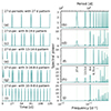 |
Fig. B.4. Time series (left column) and corresponding periodograms (right column) for 27 d-periodic test signals with a different pattern of spikes per period. The spectral peaks mark the 27 d-period and its harmonics. |
The first example (a) shows a 27 d-periodic signal consisting of a single spike, akin to a single, long-lasting CIR. The corresponding power spectrum (b) shows peaks at the primary and all harmonics of the 27 d-frequency. All peaks have roughly the same power. This is expected; it is well known that the Fourier spectrum of a Dirac comb is itself a Dirac comb (e.g. VanderPlas 2018).
In the second example (c-d) another spike was added to the periodic signal; the spikes occur in an alternating pattern of eight and nineteen days, abbreviated as an 8-19 pattern. The amplitude of the spikes is the same as in the first example. The periodogram shows peaks at the same frequencies; however, their power is distributed differently. The first harmonic (13.5 d) has become less powerful and the second and third harmonics have become more powerful than the primary peak, for example.
The relative power of the peaks depends on the phase shift between the spikes. If the spikes occur close to each other (e.g. a 2-25 pattern), the primary frequency remains the most powerful peak and the power decreases for higher harmonics. If the spikes are equidistant, the signal becomes 13.5 d-periodic; for a 13-14 pattern (e-f), the 13.5 d peak and all other odd harmonics of the 27 d are powerful, whereas the primary and all even harmonics almost vanish.
In the fourth and fifth examples (g-j), a third spike per period has been added. Similar to the case of two spikes per period, if the spikes are unevenly distributed among the period, the powers are unevenly distributed: if the spikes occur closely together, the primary frequency is powerful and the power decreases for higher harmonics (g-h); if the spikes are evenly distributed, the signal becomes 9 d-periodic, so only the second harmonic and every successive third harmonic remain, whereas all other harmonics and the primary peak vanish (i-j).
Thus, assuming that CIRs cause spike-like features in the time series, for example by reducing or enhancing detections of dust particle impacts, the number of CIRs and how they are spatially distributed among one solar rotation will affect the powers of the solar rotation signatures. The spectral signature of a reduction or an enhancement are indistinguishable in a periodogram.
B.4. Identification of CIRs
CIRs are usually not identified directly as cohesive, co-rotating structures but as individual SIRs that pass by a spacecraft (see Sect. 2.4). The dataset by Jian et al. (2006), Jian (2021), for example, used measurements made with Wind and with the Advanced Composition Explorer to identify these individual SIRs. Although the dataset contains a flag that indicates whether the respective SIR is part of a CIR, it does not assign these SIRs to specific CIRs. Therefore, the dataset contains no identification of CIRs nor any indication on their number of co-rotations. Similarly, the dataset by Hajra & Sunny (2022) only contains a list of individual SIRs without any indication of CIRs. To identify CIRs in these datasets, it is therefore necessary to identify which SIRs are part of CIRs.
If a SIR succeeds another SIR by roughly a Carrington rotation period, it is likely that both SIRs are the same recurring structure that co-rotates with the Sun, which is then identified as a CIR. Using the two datasets of individual SIRs, a set of SIRs were identified as a CIR if all constituent SIRs occurred at multiples of a Carrington rotation period, T = n ⋅ TC, n ∈ ℕ, to each other, where TC = 27.2753 d, allowing for some slack, T ± tsl.
This method will not perfectly identify every CIR correctly: if two unrelated SIRs accidentally occur within T ± tsl, they will falsely be recognised as belonging to the same CIR. If, for any reason, a single SIR during a long-lasting CIR is not detected, the CIR will be identified as two unrelated CIRs. Different choices of tsl lead to different sets of CIRs. If a SIR could ambiguously be related to two CIRs that are unrelated amongst themselves, the SIR is assigned to the earlier CIR even if it were naturally part of the second one.
In practice, a SIR was recognised as part of a potential CIR if it fulfilled two criteria:
-
1.
the individual SIR had to occur within TC ± 3 d after the previous SIR that is part of the potential CIR, and
-
2.
the individual SIR had to occur within n ⋅ TC ± 5 d, n ∈ ℕ of all other previous SIRs that are part of the same CIR.
Applying this method lead to the list of CIRs that are displayed in Fig. 13.
B.5. Details of the interplanetary magnetic field sector structure case studies
This appendix presents case studies for the IMF sector structure (see Sect. 4.4). The list of sector structure polarities by Svalgaard (2023b) gives the polarity of the IMF at Earth for each day as either an “X” (negative polarity, pointing towards the Sun), as a period (positive polarity, pointing away from the Sun), or an asterisk (mixed polarity, “zero”). To calculate power spectra of the sector structure, these values were mapped to −1, +1, and 0, respectively.
Several time periods of noteworthy sector structures can be observed: a stable four-sector structure in 2006; a chaotic structure in 2012; a stable two-sector structure in 2016; a chaotic structure from June 2020 until June 2021; and a stable two-sector structure in 2022. All of these time periods were taken to be 365 d long. If the solar rotation signatures were caused by the local IMF sector structure, clear solar rotation signatures should be observable during times of a stable sector structure, and no solar rotation signatures should be observable during times of a chaotic sector structure.
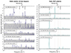 |
Fig. B.5. Periodograms for certain time periods corresponding to different sector structures of the IMF, the daily number of dust impacts with morphological types A and B (left, indigo curves), and the sector boundary structure (right, teal curves). All selected time periods last 1 yr. The axes of the periodogram amplitude are scaled identically within each column. The vertical lines are as in Fig. 14. The estimated 95% significance thresholds are indicated by grey shaded areas. |
The periodograms for the respective time period of interest are displayed in Fig. B.5 for both the daily number of dust impacts (left column) and the daily polarity of the IMF (right column). The IMF polarity spectra feature a strong solar rotation signature at the primary peak (about 27 d) when the sector structure is in a stable two-sector configuration (2016 and 2022; c and e, respectively). When the sector structure is in a stable four-sector configuration (2006, a), the first harmonic (about 13.5 d) is most powerful and the primary peak is less powerful. When the sector structure is chaotic (2012, 2020; b and d, respectively), these features are less powerful.
The dust impact spectra show no correlation with the IMF polarity spectra or with the sector structure stability. The solar rotation signatures can be both powerful (2006, a) or weak (2016, 2022; c and e, respectively) during a stable sector structure, and also powerful (2012, b) or weak (2020-2021, d) during a chaotic structure. This indicates that there is no strong correlation between the observed dust impacts and the local IMF polarity.
B.6. Dust impacts with morphological types C and D
As mentioned in Sect. 3.3, the analyses of Sects. 3 & 4 only take into account dust impacts that generated signals with morphological types A and B. This is motivated by the unexplained features of the time series of dust impacts with types C and D before 2005, especially for the impacts observed by the x-antenna (cf. Malaspina & Wilson 2016, Fig. 5). However, since 2005, the time series of dust impacts with types C and D does not show comparably exceptional features.
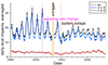 |
Fig. B.6. Daily number of dust impacts on Wind at L1 of all morphological types (black), of only types A and B (blue), and of only types C and D (red), given as a centred moving average with a width of 91 d. The events are marked the same as in Fig. 6a; the dataset has been corrected as per Sect. 3.3. |
This is shown in Fig. B.6, which compares the time-averaged daily number of dust impacts of types C and D with those of types A and B (see Fig. 6a). Generally, dust impacts with types C and D occur less frequently than those of types A and B. Furthermore, the seasonal variation of dust impacts of types C and D is considerably less apparent than for types A and B, indicating that dust particles that generate signals of types C and D may predominantly be interplanetary in nature.
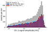 |
Fig. B.7. Amplitude distributions of all impacts (grey) with morphological types C and D measured by the y-antenna, impacts measured only when the spacecraft moved against the ISD inflow direction (February to April; blue and white), and impacts measured only when the spacecraft moved with the ISD inflow direction (August to October; red and black). The distribution of all impacts has been scaled by a factor of 0.5 to tighten the histogram’s vertical axis (see Fig. 8.) |
This is further supported by the amplitude distribution of the dust impacts with types C and D, which is shown in Fig. B.7. As in Fig. 8 for types A and B, the amplitude distributions for the three months when the spacecraft moved against or with the ISD inflow direction, respectively, are graphed as well. The distributions when moving against and with the ISD inflow direction are strikingly similar for types C and D, indicating that these dust impacts predominantly stem from IDPs. Furthermore, in contrast to the amplitude distribution of signals of types A and B, which decreases at amplitudes above A ≳ 200 mV, the amplitude distribution of types C and D increases with the amplitude over the entire amplitude range; the sudden decline at the very highest amplitudes (A > 1.5 × 10³ mV) is most likely caused by a saturation of the instrument and not a physical feature of the amplitude distribution.
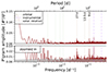 |
Fig. B.8. Periodogram of the daily number of dust impacts with morphological types C and D observed at L1, marked as in Fig. 9. The bottom panel shows a zoomed-in view of the full spectrum with the estimated 95% significance thresholds indicated by a grey shaded area. |
Figure B.8 shows the periodogram of all dust impacts with types C and D observed at L1 (see Fig. 9 for the periodogram of dust impacts with types A and B). Compared to the spectrum of types A and B, the dust impacts of types C and D are less powerful because there are fewer dust impacts with types C and D than with types A and B. The spectrum of types C and D features a significantly smaller peak at 365 d; the seasonal variation is much less apparent, once again indicating the likely interplanetary nature of these dust particles. The solar rotation signatures, however, are clearly evident for impacts of types C and D. While the solar rotation harmonics occur at periods of 13.5 d and 9 d for types C and D, same as for types A and B, the primary occurs at 27.1 d for types C and D, compared to 26.4 d for types A and B. The physical origin of this frequency shift is unknown and requires further investigation.
One hypothesis for the origin of impact signals of types C and D is that they stem from extremely abrupt signals that are smoothed to the C and D morphologies by the Wind/WAVES instrument. It is possible that only the highest-amplitude impacts can be smoothed to C and D impact signals, which would explain the odd amplitude distribution (see Fig. B.7). This motivates excluding C and D impact signals for all analyses where the amplitude is of relevance. Another possibility is that C and D impact signals are not caused by dust signals at all; this motivates excluding C and D impacts outright. However, because the frequency analysis of C and D impacts (see Fig. B.8) does show the solar rotation signatures, the veracity of this hypothesis is uncertain. Further investigation is required.
This analysis of dust impacts with morphological types C and D shows that both the time evolution, especially the seasonal variation, and the amplitude distribution of these dust impacts differs from those of types A and B. This motivates taking into account only dust impacts of types A and B for the analyses in Sects. 3 and 4. However, the solar rotation signatures are evident for types C and D as well as for types A and B.
Appendix C: Methodology of the scaled superposed epoch analysis
The systematic reduction of dust impact observations during SIRs since 2005 has been investigated in Sect. 4.3.1 by a superposed epoch analysis (Chree 1913). SIRs were taken from the datasets by Jian et al. (2006), Jian (2021) and Hajra & Sunny (2022). The dataset by Jian et al. (2006), Jian (2021) differentiates between SIRs that are part of CIRs and SIRs that do not recur; only the SIRs that are associated with CIRs were taken into account. All events from the Hajra & Sunny (2022) dataset were included. The SIR datasets contain an initial and a final timestamp of each SIR, which determine the duration of the respective SIR.
By superposition, the rate of dust impacts of all morphological types during all SIRs was compared to the rate of dust impacts in the preceding and following time intervals. The superposed epoch analysis was performed as follows:
-
The time intervals that precede (follow) the SIRs were each 2 d long, ending (beginning) with the initial (final) timestamp of the respective SIR.
-
The duration of each individual SIR was given by the initial and final timestamps from the datasets. Because these durations vary for the different SIRs, they were rescaled to the average duration, which is ∼1.42 d (see Fig. 12a).
-
The timestamps of all dust impacts were reduced to the same time interval, i.e. all SIRs were superposed, beginning and ending at the same rescaled time.
-
To calculate the number of dust impacts per day, first the number of dust impacts during a given time interval must be known. Therefore, a moving average, Nd(t), with a window width of either Δt = 4 h or Δt = 30 min was calculated over the superposed SIR, containing the total number of dust impacts during the sliding window, summed over all rescaled SIRs.
-
The extrapolated number of dust impacts per day, n(t) = Nd(t)/(NSIRΔt), is the total number of dust impacts, Nd(t), divided by the number of SIRs, NSIR, and the duration of the sliding window, Δt.
-
Measurement gaps were taken into account by rescaling: if a measurement gap of duration tgap occurred during an event of total duration tdur, the duration of the sliding window was rescaled to (Δt)scal = Δt ⋅ (tdur−tgap)/tdur.
Figure 12a shows the results of this scaled superposed epoch analysis of the dust impacts during SIRs for sliding windows of 30 min and 4 h, including intervals of 95% confidence. This confidence interval corresponds to the interval within ±1.95σ around the distribution’s mean, n(t), where  is the standard deviation of the average number of dust counts within the respective time window.
The strength of the reduction or enhancement of dust impacts was quantified by dividing the average rate of dust impacts during the superposed SIR, ndur, by the average rate of dust impacts in the preceding and following time intervals, nprc + flw. Its uncertainty corresponds to ±1.95σ, where  with
with  for i ∈ {dur; prc + flw}, and Ni is the total amount of dust impacts measured during all SIRs or in all preceding and following time intervals. This method has been validated with synthetic data and applied in-depth to the dust impacts observed by Wind by Péronne et al. (in prep.).
All Figures
|
Fig. 1. Relevant dust properties versus particle mass. Top panel: β-ratio versus particle mass following the astronomical silicates of Gustafson (1994) adapted to have a maximum of β = 1.6 (Sterken et al. 2013). Middle panel: Subsequent heliocentric speed of ISD particles (solid black curve) dependent on the particle mass using Eq. (4); Earth’s orbital speed (dashed blue line) for comparison. Bottom panel: Signal amplitude of a single dust particle, taken as m v3.5 as per Eq. (3), for an IDP with an impact speed of 20 km/s (solid magenta line), a β-meteoroid of 50 km/s (dash-dotted blue line), and an ISD particle in March (dashed red curve) and in September (dotted green curve). No line was plotted for β-meteoroids above m > 10−16 kg because β-meteoroids are constrained to lower masses (Wehry & Mann 1999; Moorhead 2021). The secondary horizontal axis of the top panel gives the particle radius, assuming spherical and compact particles with a density of 2500 kg/m3 (Sterken et al. 2013). ISD with β > 1.38 (dashed blue horizontal in the top panel) cannot reach Earth’s orbit; it is excluded (grey-shaded area). |
| In the text | |
|
Fig. 2. Schematic drawing of the actively used Wind/WAVES antennas (thick blue lines) on the Wind spacecraft (grey and gold cylinder), not drawn to scale. The majority of the X+-arm was cut in 2000 and 2002 (dotted red line). |
| In the text | |
|
Fig. 3. Signal amplitude of a single dust particle, taken as m v3.5 as per Eq. (3), for an interstellar (solid curves) and interplanetary (dashed horizontal lines) dust particle and a β-meteoroid (dotted horizontal lines) of mass m = 10−18 kg (yellow lines), m = 10−17 kg (red lines), m = 10−16 kg (purple lines), m = 10−15 kg (violet lines), and m = 10−14 kg (indigo lines). The ISD with m = 10−16 kg (solid purple curve) cannot reach 1 AU due to its high β-ratio; thus, this curve is not visible. No lines were plotted for β-meteoroids above m > 10−16 kg. For more details, see Sect. 3.2.2. |
| In the text | |
|
Fig. 4. Differential flux of IDPs following the Grün flux (solid blue curve) and ISDs derived from the MRN flux (dashed red curve). The faint dotted lines indicate the deviation from the power law df/dm ∝ m11/6. |
| In the text | |
|
Fig. 5. Stylised waveforms for the four morphological phenotypes of dust impact signals measured by the TDSF. Only impacts that generated single-spike signals (left panel, types A and B) are taken into account for the analyses. Reproduced with permission after Malaspina & Wilson (2016, Fig. 2); copyright of the original figure by John Wiley and Sons. |
| In the text | |
|
Fig. 6. Dust impacts observed by Wind versus time. Top panel: Daily number of dust impacts on Wind at L1 that generated signals of morphological types A and B, given for each day (blue discs) and as a centred moving average with a width of 91 d (black line). For comparison, yellow diamonds mark the moving average flux on 25 March of each year, which is close to each annual maximum. The sampling rate was periodically changed beginning in April 2011, marked by a vertical dotted pink line, making the instrument insensitive to dust impacts for roughly two days every six days. Larger time periods where the instrument was inoperable in regard to measuring dust impacts occurred in 2013 (shaded orange, “z-trigger”) and in late 2014 (shaded red, “system outage”). The increase and decrease of dust impacts due to the solar magnetic cycle is indicated by diagonal grey arrows. The dataset has been corrected for these instrumental effects as per Sect. 3.3 (see Appendix A). Bottom panel: Daily number of dust impacts observed by Wind as a 91 d centred moving average (black curve, identical to the top panel) compared to the numerically simulated particle flux of ISD at Wind’s orbital position, vertically offset by an assumed constant IDP flux of 10 #/d. (For more information on the simulations, see Sect. 3.4.1). |
| In the text | |
|
Fig. 7. Time series for all dust impacts of morphological types A and B with a y-antenna signal amplitude below 19.2 mV (blue) and above 240 mV (red), graphed as a centred moving average with a width of 91 d. The two amplitude selections each correspond to 20% of all impacts. |
| In the text | |
|
Fig. 8. Amplitude distributions of all impacts (grey bars) with morphological types A and B measured by the y-antenna, impacts measured only when the spacecraft moved against the ISD inflow direction during February, March, and April (shown with blue filled bars outlined in white), and impacts measured only when the spacecraft moved with the ISD inflow direction during August, September, and October (shown with red filled bars outlined in black). The distribution of all impacts has been scaled by a factor of 0.5 to tighten the histogram’s vertical axis. The vertical dashed green lines indicate every 20th percentile of the signal amplitude; the weakest and the strongest 20% of all impact signals were selected when generating Fig. 7. |
| In the text | |
|
Fig. 9. Periodogram of the daily number of dust impacts with morphological types A and B recorded at L1. The periodogram was evaluated at the DFT’s natural frequencies and oversampled by a factor of 15. The three most relevant frequencies and their harmonics are marked by vertical lines: the 365 d-period corresponding to the orbital period of the spacecraft (dotted green lines), the 6 d-period introduced by instrumental effects (dashed purple lines), and the solar rotation period at 27 d (solid brown lines). The bottom panel shows a zoomed-in view of the full spectrum with the estimated 95% significance thresholds indicated by a grey shaded area. |
| In the text | |
|
Fig. 10. Periodograms of the daily number of dust impacts with morphological types A and B for the three months of each year that correspond either to the orbital segment against the ISD inflow (February to April, blue curve, top panel) or with the ISD inflow direction (August to October, red curve, bottom panel). The two panels are scaled identically; the estimated 95% significance thresholds are indicated by grey shaded areas. Frequencies of interest are marked by vertical lines as in Fig. 9. |
| In the text | |
|
Fig. 11. Periodograms of the daily number of dust impacts with morphological types A and B during six years in the focusing phase (2007–2012, blue curve, top panel) and six years in the defocusing phase (September 2017 to August 2023, red curve, bottom panel). The two panels are scaled identically; the estimated 95% significance thresholds are indicated by grey shaded areas. Frequencies of interest are marked by vertical lines as in Fig. 9. |
| In the text | |
|
Fig. 12. Reduction and enhancement of dust impact detections made by Wind during SIRs. Top panel: Scaled superposed epoch analysis of the daily number of dust impacts during SIRs as a moving average within a 30 min interval (grey) or a 4 h interval (red). Only the SIRs that are associated with CIRs were taken into account. The shaded red area indicates 95% confidence intervals for a Poissonian distribution. Bottom panel: Histogram of the enhancement or reduction factor of dust impacts for the SIRs that are associated with CIRs. The dashed blue line denotes the average reduction of 20.7%. The five SIRs that begin on 1 January 2005, 23 November 2006, 15 January 2007, 24 November 2008, and 30 August 2009 were excluded due to low number statistics. |
| In the text | |
|
Fig. 13. CIRs identified by the method proposed in Sect. 4.3.2 for the SIR datasets of Jian et al. (2006), Jian (2021) since 2005 (top panel) and Hajra & Sunny (2022) (bottom panel). Each horizontal bar corresponds to one CIR. Time intervals of interest have been highlighted by shaded areas. We note that the two datasets overlap only for the years 2008 and 2009. |
| In the text | |
|
Fig. 14. Periodograms for certain time periods corresponding to different systematic rates of occurrence of CIRs for the daily number of dust impacts with morphological types A and B (left, indigo curves) and of a synthetic time series of dust impacts with an absolute dust depletion by SIRs (right, teal curves; see Sect. 4.3.3). All of the selected time periods are nine months long; their initial and final dates are given as doy. All panels in the left column share the same axis range and scale for easier comparison. The panels in the right column are scaled differently. Frequencies of interest are marked by vertical red lines as in Fig. 9, including the third solar rotation harmonic at 6.75 d; the 6 d-periodicity has only been marked in the dust impact spectra since 2011. Estimated 95% significance thresholds are indicated by grey shaded areas. |
| In the text | |
|
Fig. 15. Synthetic time series of IDP and ISD impacts on Wind following Eq. (6) to reproduce the observed number of impacts in Fig. 6a. The times at which the oscillations due to the solar magnetic cycle and the annual variation are at their maxima are indicated by a vertical dashed red line and a vertical dotted purple line, respectively. |
| In the text | |
|
Fig. 16. Periodogram of Wind’s floating potential from 2005 to 2021 using Method 4 of Wilson et al. (2023a) for parallel pitch angles (cf. Wilson et al. 2023a, Fig. 6). The data were averaged over each day before generating the spectrum. The vertical lines are as in Fig. 9. The estimated 95% significance thresholds are indicated by a grey shaded area. |
| In the text | |
|
Fig. 17. Scaled superposed epoch analysis (top panel) and histogram of the reduction or enhancement during each event (bottom panel) of Wind’s floating potential during all SIRs that are associated with CIRs since 2005, in analogy to Fig. 12. The shaded red confidence band in the top panel corresponds to the standard deviation and a 1 V measurement uncertainty for individual measurements of the floating potential. The first fourteen SIRs of 2005 were not taken into account because no spacecraft floating potential data was available. |
| In the text | |
|
Fig. A.1. Unprocessed data presented as the daily number of impacts. Each pale blue disc corresponds to the number of impacts during one calendar day; a moving average within a centred window of 91 d is given by the black line. The many external influences (see Appendix A.1), marked by vertical lines and shaded areas, are not taken into account in this representation of the unprocessed data. |
| In the text | |
|
Fig. A.2. Amplitude distribution of type A and B dust impact signals before the first antenna break on 8 August 2000 (top row) and after the second antenna break on 9 September 2002 (bottom row) for the x-antenna (Channel 1; left column) and for the y-antenna (Channel 2; right column), separated into positive (blue) and negative (red) amplitudes. |
| In the text | |
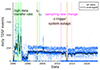 |
Fig. A.3. Daily number of TDSF events. The figure is displayed in the same manner as Fig. A.1. |
| In the text | |
|
Fig. A.4. Daily number of dust impacts and TDSF events, corrected for the sampling rate change in April 2004. Top panel: Daily number of dust impacts (left) and daily number of TDSF events (right) as moving averages with centred windows of 91 d. The red curves depict the “raw” data – same as in Figs. A.1 and A.3 but additionally taking into account the data gaps of 2013 and 2014, which are marked by grey bars. The blue curves depict the same data but corrected for the change of the sampling rate in April 2011, which is marked by a vertical dotted magenta line. Bottom panel: Daily number of dust impacts normalised by the daily number of TDSF events, graphed for each individual day (blue discs) and as a moving average with a centred window of 91 d (black curve). The data have been corrected for the sampling rate change and the data gaps. |
| In the text | |
|
Fig. A.5. Distance of the spacecraft to Earth (smooth blue curve; left vertical axis) and normalised daily dust impacts (jagged red curve; right vertical axis) with a centred moving average of 45 d. The time intervals when the high data transfer rate was in use and the times spent at the Lagrange points are indicated by shaded areas. The distance to Earth is given in Earth radii, 1 Re ≈ 6378 km. |
| In the text | |
|
Fig. B.1. WWZ periodogram of the daily number of dust impacts recorded at L1, in analogy to Fig. 9. The bottom panel shows a zoomed-in view of the full spectrum, with the estimated 95% significance thresholds indicated by a grey shaded area. |
| In the text | |
|
Fig. B.2. Superposed epoch analysis of all gaps stemming from the 6 d-periodic sampling rate change; serial number of the gaps versus time since the start of the two days of removed data. Each dot corresponds to one observed dust impact; each line of identically coloured dots corresponds to the same epoch, i.e. gap serial number. The vertical dashed black lines correspond to the reported timing of the sampling rate change. |
| In the text | |
|
Fig. B.3. Periodogram of the daily number of dust impacts with morphological types A and B before April 2011, original data (blue curve, top panel) and data with artificially induced 6 d-periodic gaps (orange curve, bottom panel), evaluated at the DFT’s natural frequencies and oversampled by a factor of five. The two panels are scaled identically. Frequencies of interest are marked by vertical lines, as in Fig. 9. The estimated 95% significance thresholds are indicated by grey shaded areas. |
| In the text | |
|
Fig. B.4. Time series (left column) and corresponding periodograms (right column) for 27 d-periodic test signals with a different pattern of spikes per period. The spectral peaks mark the 27 d-period and its harmonics. |
| In the text | |
|
Fig. B.5. Periodograms for certain time periods corresponding to different sector structures of the IMF, the daily number of dust impacts with morphological types A and B (left, indigo curves), and the sector boundary structure (right, teal curves). All selected time periods last 1 yr. The axes of the periodogram amplitude are scaled identically within each column. The vertical lines are as in Fig. 14. The estimated 95% significance thresholds are indicated by grey shaded areas. |
| In the text | |
|
Fig. B.6. Daily number of dust impacts on Wind at L1 of all morphological types (black), of only types A and B (blue), and of only types C and D (red), given as a centred moving average with a width of 91 d. The events are marked the same as in Fig. 6a; the dataset has been corrected as per Sect. 3.3. |
| In the text | |
|
Fig. B.7. Amplitude distributions of all impacts (grey) with morphological types C and D measured by the y-antenna, impacts measured only when the spacecraft moved against the ISD inflow direction (February to April; blue and white), and impacts measured only when the spacecraft moved with the ISD inflow direction (August to October; red and black). The distribution of all impacts has been scaled by a factor of 0.5 to tighten the histogram’s vertical axis (see Fig. 8.) |
| In the text | |
|
Fig. B.8. Periodogram of the daily number of dust impacts with morphological types C and D observed at L1, marked as in Fig. 9. The bottom panel shows a zoomed-in view of the full spectrum with the estimated 95% significance thresholds indicated by a grey shaded area. |
| In the text | |
Current usage metrics show cumulative count of Article Views (full-text article views including HTML views, PDF and ePub downloads, according to the available data) and Abstracts Views on Vision4Press platform.
Data correspond to usage on the plateform after 2015. The current usage metrics is available 48-96 hours after online publication and is updated daily on week days.
Initial download of the metrics may take a while.