| Issue |
A&A
Volume 698, June 2025
|
|
|---|---|---|
| Article Number | A138 | |
| Number of page(s) | 31 | |
| Section | The Sun and the Heliosphere | |
| DOI | https://doi.org/10.1051/0004-6361/202453532 | |
| Published online | 06 June 2025 | |
Interstellar dust measured in situ by Ulysses: New aspects of the particle size distribution and its modulation by the heliosheath
1
ETH Zürich, Institute for Particle and Astroparticle Physics, 8093 Zürich, Switzerland
2
Freie Universität Berlin, Institute of Geological Sciences, 12249 Berlin, Germany
3
MPI für Sonnensystemforschung, 37077 Göttingen, Germany
4
Planetary Exploration Research Center, Chiba Institute of Technology, Narashino, Chiba 275-0016, Japan
5
University of Applied Sciences and Arts Northwestern Switzerland, School of Engineering, 5210 Windisch, Switzerland
⋆ Corresponding author: This email address is being protected from spambots. You need JavaScript enabled to view it.
Received:
19
December
2024
Accepted:
10
April
2025
Abstract
Interstellar dust (ISD) enters the heliosphere from the direction of its nose. It is first modulated by the heliosheath and then the inner heliosphere before it is measured by the dust detectors on board of spacecraft, for example on Ulysses. Various criteria exist to distinguish ISD from the dust of other sources, and different methods exist to determine the particle masses and impact speeds from the measurements.
Key words: Sun: heliosphere / interplanetary medium / dust / extinction / ISM: general
© The Authors 2025
 Open Access article, published by EDP Sciences, under the terms of the Creative Commons Attribution License (https://creativecommons.org/licenses/by/4.0), which permits unrestricted use, distribution, and reproduction in any medium, provided the original work is properly cited.
This article is published in open access under the Subscribe to Open model. This email address is being protected from spambots. You need JavaScript enabled to view it. to support open access publication.
1. Introduction
Impacts of interstellar dust (ISD) grains on the Ulysses spacecraft allowed for the first successful in situ measurement of ISD (Grün et al. 1993). Long-term measurements of ISD with Ulysses and comparisons with numerical simulations (Landgraf 1998; Sterken et al. 2015) have since revealed previously unknown details of ISD. For example, Krüger et al. (2015) have analysed the ISD mass distribution in the Solar System and inferred the gas-to-dust mass ratio in the local interstellar medium (LISM), while Strub et al. (2015) have investigated the ISD time-variability due to the solar magnetic cycle and observed a change in the ISD flow direction in 2005–2006.
Ulysses’ orbit was highly inclined with respect to the Solar System’s ecliptic plane (Wenzel et al. 1992), in which interplanetary dust particles (IDPs) are predominant (e.g. Grün et al. 1997). The spacecraft’s orbital plane was oriented almost perpendicular to the inflow direction of ISD. Because zodiacal dust predominantly moves on prograde orbits, it can be easily distinguished from ISD during the majority of Ulysses’ orbit. Only close to the spacecraft’s perihelion did the direction of motion of ISD coincide with the direction of motion of particles on prograde orbits (Strub et al. 2015).
One difficulty when investigating ISD is to distinguish it from IDPs. The impact ionisation detector on board Ulysses (Grün et al. 1992) in combination with thorough calibrations (Göller & Grün 1989) allows for a reconstruction of the impact speed as well as the mass of the impacting particle (Grün et al. 1995a). Alongside the directionality of the impacting particle, which is approximately known from the detector boresight during the particle impact and the opening angle of the detector, the ability to reconstruct these aspects has allowed multiple sets of criteria to be established by which ISD can be discriminated from other dust species such as IDPs (Landgraf et al. 2003; Krüger et al. 2015; Strub et al. 2015). These different sets of criteria were devised to minimise biases for different types of analyses. As such, depending on the set of criteria, different biases are also induced on the resulting data subsets, and they may influence the ISD properties inferred from the Ulysses data (e.g. its particle flux, flow direction, or mass distribution) in different ways. Furthermore, different methodologies have been devised to determine the masses of the impacting dust particles (Grün et al. 1995a; Landgraf 1998; Krüger et al. 2015). These either depend entirely on properties of the impact signals measured by the detector or assume properties of the particles’ trajectories, such as the particle speed.
In this work, we investigate the different ISD selection criteria and mass determination methods. Our aim is to research the following: (1) how the choice of the ISD selection criteria influences the derived ISD particle flux or directionality, and (2) how the choice of the mass determination method influences the inferred ISD mass distribution.
The inferred gas-to-dust mass ratio in the LISM is dominated by the most massive ISD particles that were measured by Ulysses (Krüger et al. 2015). Furthermore, ISD particles of high mass are affected less by the Lorentz force within the heliosphere than lower-mass particles; they are not deflected from their trajectories as strongly (Sterken et al. 2012a). Thus, the most massive ISD particles are of particular relevance when investigating the direction of origin of the ISD. For example, if Ulysses had measured an additional interstellar inflow of dust particles that does not agree with the nominal ISD inflow direction1, it would indicate another direction of origin of ISD particles, for example from within the G cloud (e.g. Redfield & Linsky 2008; Linsky et al. 2019, 2022a,b; Swaczyna et al. 2022).
For these reasons, we investigated the most massive ISD particles identified by Ulysses. Our aim is to research the following: (1) whether these most massive ISD particles are unambiguously interstellar or could have a different origin, (2) how this affects the inferred gas-to-dust mass ratio of the LISM, and (3) how the choice of the mass determination method influences this gas-to-dust mass ratio.
Before ISD particles can be measured by Ulysses or other in situ detectors within the Solar System, they must traverse both the heliosheath and the inner heliosphere, both of which modulate the size distribution of ISD. The modulation in the inner heliosphere can be numerically modelled (Landgraf 1998; Sterken et al. 2015; Strub et al. 2019), whereas the filtering by the heliosheath is less accurately known (Linde & Gombosi 2000; Slavin et al. 2012).
If a size distribution of ISD before it traverses the heliosphere is assumed, the size distribution measured by Ulysses in combination with numerical simulations of the inner heliosphere modulation can be used to infer the filtering in the heliosheath. This is illustrated and has been performed in this publication, for which we assumed an original ISD size distribution inferred from astronomical measurements (‘MRN distribution’; Mathis et al. 1977). The results of such an analysis can be used to generate predictions for the ISD environment that other spacecraft have encountered or will encounter, for example for DESTINY+ (Arai & DESTINY+ Team 2024; Hunziker et al., in prep.).
We introduce ISD and the Ulysses mission in Sect. 2, and we present the different ISD selection criteria and mass determination methods in Sects. 3 and 4, respectively. After investigating the research questions in Sects. 5, 6, and 7, we draw conclusions in Sect. 8.
2. Theoretical background
This section introduces the most relevant aspects of the physical forces that affect ISD in the heliosphere (Sect. 2.1) and of the Ulysses mission (Sect. 2.2). A detailed review of the former is given by, for example, Sterken et al. (2012a, Sterken et al. (2019). More information on the latter is given by, for example, Wenzel et al. (1992).
2.1. Trajectories of interstellar dust in the heliosphere
The Solar System moves with a relative speed of 26 km/s (Wood et al. 2015) through the surrounding Local Interstellar Cloud (LIC) in the direction of the G cloud (Redfield & Linsky 2008). Currently, it may reside in a mixed-cloud interstellar medium (ISM) in-between the LIC and the G cloud (Swaczyna et al. 2022).
It was concluded by Grün et al. (1993, 1994) that the inflow direction of ISD (from the retrograde direction at Ulysses’ aphelion) is compatible with the interstellar upstream direction and the helium inflow direction, which was also determined by Ulysses (Witte et al. 1993). This has been verified by Landgraf (1998). Krüger et al. (2015) confirmed an average impact speed of the dust grains on Ulysses of (24 ± 12) km/s. Throughout this work, we assumed that ISD homogeneously enters the heliosphere with the helium inflow, which comes from the direction of (lHe, bHe) = (255.41°, 5.03°) and with an ISD speed of ca. vISD, ∞ = 26 km/s (Swaczyna et al. 2018, 2023).
As these charged ISD particles travel through the magnetic field in the plasma interaction region of the Sun with the LISM, the so-called heliosphere (e.g. Richardson et al. 2023), they are filtered and modulated in different regions of the heliosphere by the Lorentz force. On their trajectories to the inner Solar System ISD particles must first cross the heliopause, which is the boundary between solar and interstellar plasma, and afterwards the termination shock, at which the solar plasma is abruptly decelerated and the interplanetary magnetic field diverges from a Parker spiral (Parker 1958). The region between the heliopause and the termination shock is called the (inner) heliosheath.
Inside the termination shock, meaning within the inner heliosphere, the forces that strongly affect ISD are well known (Sterken et al. 2012a): solar gravitation, FG; solar radiation pressure, FSRP; and the Lorentz force, FL. Because the first two forces are both radial and both follow an inverse square law with respect to the heliocentric distance, their ratio, β = |FSRP|/|FG|, depends only on particle properties such as the mass, geometric cross section, and optical absorption and scattering efficiency. The Lorentz acceleration depends on the particle’s charge-to-mass ratio, Q/m. Together, the parameter set of (β, Q/m) is used to define different dust species in dynamical ISD simulations (Landgraf et al. 2000; Sterken et al. 2012a, 2013, 2015).
The relation between β and the particle mass, m, is described by a β-curve that depends on particle properties such as composition and morphology via its optical properties. Fig. 1 shows the calculated β-ratio against the mass for different particle compositions and porosities (see Gustafson 1994; Kimura & Mann 1999). Unless otherwise specified, we used the adapted astronomical silicates with a particle density of ρd = 2500 kg/m3 throughout this work (see Sterken et al. 2012a).
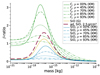 |
Fig. 1. β-curves for amorphous carbon (‘C’, green lines, Kimura & Mann 1999), astronomical silicates (“SiO”, solid gold line, Gustafson 1994; and blue lines, Kimura & Mann 1999), and adapted astronomical silicates (“ad. SiO”) with an assumed dust density of ρd = 2500 kg/m3 (thick dashed maroon line; Sterken et al. 2012a). The β-curves of Kimura & Mann (1999) have porosities, p, ranging from 0% (compact particles) to 93% (fluffy particles), indicated by different line styles. (After Sterken et al. 2015, Fig. 2.) |
When β is greater than one, solar radiation pressure dominates over solar gravitation, and the ISD particles are deflected away from the Sun. Depending on how large the ISD particles’ β-ratio is, they cannot reach a paraboloid region around and behind the Sun, as seen from the ISD inflow direction. These exclusion zones are referred to as β-cones; for a given βmax only particles with smaller β < βmax can penetrate into these cones (see, e.g. Landgraf et al. 1999; Altobelli 2004). If a spacecraft’s orbit lies (partially or entirely) within a β-cone corresponding to βmax, the mass distribution of the ISD particles that impact the spacecraft will feature a gap that corresponds to the particles with β > βmax, the so-called β-gap.
2.2. The Ulysses mission
The Ulysses spacecraft was launched on 6 October 1990. After a swing-by manoeuvre at Jupiter in February 1992, it traversed the Solar System at an inclination of 79°, almost perpendicular to the ecliptic plane (Wenzel et al. 1992). The orbit of Ulysses is depicted in three dimensions in Fig. 2 and has been projected onto the heliocentric ecliptic coordinate xz- and yz-planes in Fig. 3.
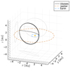 |
Fig. 2. Three-dimensional depiction of the orbits of Ulysses (solid black line), Jupiter (dashed ochre line), and Earth (dash-dotted blue line) in heliocentric ecliptic coordinates. The +x-direction points towards the vernal equinox, and the +z-direction points to ecliptic north. The Sun is marked as a yellow star. The faint grey curves on the coordinate planes are projections of Ulysses’ orbit onto that plane (see Fig. 3). The dark grey lines close to the almost-horizontal and vertical axes are projections of the homogeneous ISD inflow coming from (l, b) = (255.41° ,5.03° ) onto the xy- and xz-planes. (See Krüger et al. 2015, Fig. 1.) |
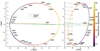 |
Fig. 3. Ulysses orbit projected onto the xz- (left) and yz-plane (right), colour-coded according to heliocentric speed. Jupiter’s and Earth’s orbits are indicated as dashed green and dotted blue lines, respectively. The dark grey arrows indicate projections of the ISD inflow direction and are identically scaled in both panels. (See Landgraf 1998, Fig. 2.5.) |
Ulysses measured cosmic dust with a multi-coincidence impact ionisation detector (Grün et al. 1992). A hypervelocity impact on the detector’s target generated electric charges of both electrons and ions (Raizer 1960), and the amplitudes and rise times of the corresponding signals were measured. With aid of thorough calibration measurements (Göller & Grün 1989), the impact speed and mass of the impacting particle could be reconstructed (Grün et al. 1995a).
The dust detector was continuously active from 28 October 1990 until 30 November 2007, barring a few short time intervals that are listed in Table B.1 (see Krüger et al. 2010, Table 1); this is illustrated in Fig. 4. The surface area of the detector was 0.1 m2. However, the effective sensitive surface area for measuring ISD depends on both the boresight direction and the field of view of the detector as well as on the relative speed between the spacecraft and the dust particle. At high relative speeds, the effective sensitive surface area can be larger than the detector’s physical surface area2, ranging from 0 m2 ≤ Aeff < 0.15 m2 (cf. Appendix B.1).
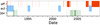 |
Fig. 4. Uptime of the dust detector with respect to measuring ISD covering the full duration of the Ulysses mission. Shaded areas denote times when the dust detector was turned off (‘off’, top row, red), when data were excluded due to time spent in the ecliptic plane (‘ecl’, middle row, blue), and when data were excluded due to Jovian streams (‘Jov’, bottom row, green). |
The Ulysses spacecraft was spin-stabilised and its spin axis perpetually pointed towards Earth to ascertain stable communications via the high-gain antenna. The boresight of the dust detector rotated about this spin axis with approximately five revolutions per minute (Wenzel et al. 1992). The boresight of the detector can be described by the rotation angle, ϕrot, which gives the phase of the spacecraft’s spin. The two-dimensional pointing of the detector in heliocentric ecliptic coordinates thus must be reconstructed from the rotation angle and the vector of the spin axis at the time of impact. This is outlined in Appendix A.
3. Distinguishing ISD from IDPs and Jovian dust streams
Detailed information of every dust impact measured by the Ulysses dust instrument is publicly available in Grün et al. (2010)3. The dataset contains 6719 events, many of which are IDPs or particles from Jovian dust streams.
3.1. Excluding Jovian dust and IDPs from the dataset
One of the challenges of processing this dust dataset is to identify which events correspond to impacts of ISD, and which stem from IDPs or Jovian dust stream particles. During some sections of Ulysses’ orbit, for example when both ISD and IDPs come from roughly the same direction during Ulysses’ perihelion, it is not possible to unambiguously identify ISD. Therefore, certain time spans have been excluded entirely from the ISD dataset. There are three such general exclusion criteria (Krüger et al. 2015):
-
All events preceding Ulysses’ Jovian flyby on 8 February 1992 have been excluded because Ulysses was in the ecliptic plane.
-
All events recorded during Ulysses crossings of the ecliptic plane at the spacecraft’s perihelion (Ulysses’ ecliptic latitudes |bU| < 60° and longitudes 247° < lU < 360° & 0° < lU < 67°) have been excluded.
-
All events corresponding to Jovian dust streams have been excluded. The time spans of these encounters have been taken from Baguhl et al. (1993, Table 2) and Krüger et al. (2006a, Table 1), and all data from 25 May 2004 until (exclusive) 12 September 2004 have been excluded (see Janisch 2021, Table A.2).
Applying these criteria to the datasets reduced the number of events to 1367.
Figure 4 displays the time intervals of the dust dataset that are missing or were excluded. Of the times where the dust detector was switched off, all events prior to the calendar year 2000 are due to spacecraft anomalies where all science instruments were turned off. After 2002 the detector was switched off because of software updates or to conserve power. The exclusion intervals in the ecliptic plane correspond to the time before the Jovian flyby and the three perihelion crossings.
3.2. The different selection criteria to identify ISD
Different criteria may be used to differentiate between ISD and IDPs/Jovian dust streams in the remaining data (Janisch 2021). These criteria bias the resulting data subsets in different ways. For example, the criterion that identifies ISD by its flow direction induces a direct bias of the flow direction; the resulting subset should not be used to investigate the directionality of ISD. Instead, another criterion is used that identifies ISD by the signal amplitude. However, because low-mass ISD is strongly affected by the Lorentz force, many of these particles are deflected from the original ISD flow direction. Thus, the flow direction of this ISD subset is indirectly biased as well.
Different ISD subsets have been compiled by using different ISD selection criteria. One of the main aspects of this study is the comparison of these ISD subsets and the effect that the choice of criteria has on the analyses (Sect. 5). We studied four subsets:
-
1.
The ‘Krüger’ subset identified ISD primarily by its flow direction and was intended to be used for mass analyses. Krüger et al. (2015) propose two criteria:
-
Ia.
In all years except 2005 and 2006, the impacting particle must have come from the direction of the He inflow; that is, the detector’s rotation angle, ϕrot, must have lain within 90° of the rotation angle associated with the He inflow, ϕHe (see, e.g., Strub et al. 2015).
-
Ib.
In the years 2005 and 2006, an additional range of 40° on the positive side of the rotation angle was allowed to account for the observed change in direction: ϕrot ∈ [ϕHe − 90° ,ϕHe + 130° ].
-
II.
Electromagnetically accelerated fragments of IDPs at the solar poles (|bU|≥60°) were excluded. These grains are associated with low ion amplitudes, QI < 10−13 C, which correspond in the dataset of Grün et al. (2010) to an ion amplitude code smaller than 8. Thus, all events at latitudes |bU|≥60° with ion amplitude codes smaller than 8 were excluded.
The Krüger subset contains 952 events. Krüger et al. (2015) found 987 events. The origin of this discrepancy mostly stems from a slightly different assumed ISD flow direction for the selection criterion (1.I)4. Additionally, the exclusion criterion (iii) of the Jovian dust streams was stricter in our investigation (Janisch 2021). Criterion (1.I) selected events by their direction and thus directly biased the directionality of the resulting subset. Because low-mass ISD is more strongly deflected by the Lorentz force, the resulting ISD mass distribution was also indirectly biased (see also criterion 1.II).
-
Ia.
-
2.
The ‘Strub’ subset primarily identified ISD by the signal amplitudes as a proxy for the particle masses and was intended for directionality analyses. Strub et al. (2015) propose three criteria:
-
I.
Events of the lowest quality class (CLN = 0) were excluded as noise. Altobelli et al. (2004) found that particles with CLN ∈ {2, 3} more often come from the ISD inflow direction and thus more likely correspond to ISD particles.
-
II.
Events with low ion signal amplitudes (QI < 10−13 C; ion amplitude code < 8) were excluded. These particles are scattered across the entire range of rotation, coming from both prograde and retrograde orbits (Landgraf 1998).
-
III.
Events with impact speeds lower than half the dust inflow speed, vmsr < vISD, ∞/2, were excluded. This criterion excluded all particles with impact speeds slower than the bulk speed of interstellar dust, vISD, ∞, taking into account the error factor of the speed measurements, which is a factor of ∼2. However, Landgraf (1998) dismissed the use of this criterion because it neglects the relative velocity of the spacecraft to the ecliptic reference frame (i.e. the spacecraft’s orbital velocity). Furthermore, the criterion assumed that only a negligible amount of ISD particles is slower than the ISD bulk speed in the ecliptic reference frame, and it neglected that particles with β > 1 are decelerated as they draw closer to the Sun as well as any acceleration or deceleration by the Lorentz force.
The Strub subset contains 533 events. Strub et al. (2015) found 580 events. The discrepancy mostly stems from the stricter handling of Jovian dust streams by exclusion criterion (iii), and from different assumptions of the ISD inflow speed, vISD, ∞, for criterion (2.III). Criterion (II.2) directly biased the mass distribution of the resulting ISD subset. However, because the Lorentz force affects low-mass particles most strongly, the criterion also indirectly biased the subset’s directionality.
-
I.
-
3.
The ‘union’ subset is the union of the Krüger subset (1) and the Strub subset (2) without the speed criterion (2.III), meaning that particles with low impact speeds were not categorically excluded. The union subset contains 1064 events.
-
4.
The ‘intersect’ subset is the intersection of the Krüger subset (1) and the Strub subset (2) without the speed criterion (2.III). The intersect subset contains 517 events.
The influence of these different criteria on the inferred ISD flux, flow direction, and mass distribution has been evaluated in Sect. 5.
4. Determination of the ISD particle mass and speed
The Ulysses dust detector recorded for each impact the amplitudes and rise times of the ion and electron signals. The total emitted charge, Q, of a dust impact and therefore the measured ion and electron signal amplitude depend on the impacting particle’s mass, m, and its impact speed, v, following a power law:
 (1)
(1)
Here, k1 = 1 (Auer 2001, Ch. II.D.1), k2 ≈ 3.5 (Balogh et al. 2001, Ch. 9.2), and the proportionality constant has to be determined with laboratory calibrations (e.g. Göller & Grün 1989). With this relation, the mass can be determined from the impact speed.
Three competing methods to determine the impact speeds, and thus the particle masses, are presented here (Landgraf 1998). The canonical method derived the impact speeds from the measured signal rise times, resulting in the impact speeds and particle masses listed in the dataset. This method is presented in Sect. 4.1. Alternatively, the ISD particle speeds could be assumed in order to reduce the effects of their measurement uncertainties. A method that assumed a homogeneous ISD inflow, corresponding to β ≡ 1, is presented in Sect. 4.2. Another alternative that iteratively refined the assumed ISD inflow speed and the resulting particle mass is presented in Sect. 4.3.
The influence of the choice of the mass determination method on the ISD flux and on the ISD flow direction is investigated in Sect. 5.3. The inferred gas-to-dust mass ratio in the LISM (Sect. 6.4) is also affected by the choice of the mass determination method.
4.1. Impact speeds and particle masses directly inferred from the measurements
The impact speed of a dust particle could be determined from the rise times of the signals measured by the detector (Grün et al. 1995a, 2010). With aid of detector calibration curves, the respective dust particle’s mass could be determined from this measurement-derived impact speed and the measured impact charge (Göller & Grün 1989).
The resulting particle masses and impact speeds are tabulated in the dataset of Grün et al. (2010). Because they were derived directly from measurements without any additional assumptions, they are referred to in the following as the measurement-derived particle masses and impact speeds, mmsr and vmsr, respectively.
The dust detector on board Ulysses was only sensitive to a certain interval of signal amplitudes, which introduced a detection bias: low-mass particles could only be detected if they impacted with sufficient speed, and low-speed particles could only be detected if they had sufficient mass. Similarly, fast and high-mass particles saturated the detector. However, this saturation only occurred for two particles, neither of which were selected by the ISD criteria.
Krüger et al. (1999) note that particle impacts on detector components other than the target, for example the inner wall or the entry grid, may artificially inflate signal rise times, leading to underestimated impact speeds and overestimated particle masses. This affected events where the measurement-derived impact speed was below vmsr < 3 km/s, which featured high masses more often than low masses due to the amplitude detection threshold and Eq. (1). The true impact speeds of these particles are unknown. Thus, we used neither the measurement-derived impact speeds nor the resulting particle masses for these particles unless we explicitly specify otherwise.
This method determined the particle masses from the impact speeds with Eq. (1). Because the measurement-derived impact speeds have an error factor of ∼2, this resulted in an error factor for the particle masses of ∼23.5 ≈ 10.
4.2. ISD particle masses inferred from assumed impact speeds corresponding to β≡ 1
To reduce the uncertainty of the particle masses that was introduced in the method of Sect. 4.1 by the derived impact speeds, Landgraf (1998) proposed an alternative that instead assumed that all particles move with vISD, ∞ = 26 km/s, corresponding to ISD particles with β ≡ 1. Strub et al. (2015, Table 1) provide a conversion from the measured ion signal amplitude, Qi, to the ISD particle mass, mISD, based on the calibration curves by Grün et al. (1995a) and assuming an ISD impact speed of vStrub = 23.2 km/s. Using this approximation and rescaling to the appropriate impact speeds, vrel, Eq. (1) yields
 (2)
(2)
![Mathematical equation: $$ \begin{aligned}&\Rightarrow m_{\mathrm{ISD} }\,[\mathrm{kg}] \approx 13.465 \cdot \left(v_{\mathrm{rel} }\,[\mathrm{km/s}]\right)^{-3.5}\cdot Q_{\mathrm{i} }\,[\mathrm{C}] . \end{aligned} $$](/articles/aa/full_html/2025/06/aa53532-24/aa53532-24-eq3.gif) (3)
(3)
Further assuming β ≡ 1 and an ISD inflow speed of vISD, ∞ = 26 km/s, the relative speed of the ISD particles of the union ISD subset ranges between 26 km/s < vrel ≤ 41 km/s (see also Fig. 7).
This method reproduced the measurement-derived masses within an error interval of a factor of 10. It assumed that all ISD particles have a homogeneous ISD inflow speed, corresponding to β ≡ 1. Therefore, this method is referred to as the ‘β ≡ 1’ method. Any acceleration or deflection of the ISD particles, for example by solar gravitation, solar radiation pressure, or the Lorentz force, was neglected. Furthermore, this method assumed that all particles are ISD; unlike the measurement-derived method presented in Sect. 4.1 it would yield erroneous results for particles of other origins.
4.3. Iterative calculation of the ISD particle speed and mass
The method in Sect. 4.2 could be refined by replacing the heliocentric ISD inflow speed, vISD, ∞, with the local ISD speed, assuming a β-ratio that corresponds to the particle’s mass (see Fig. 1):
 (4)
(4)
where vISD, ∞ = 26 km/s is the homogeneous ISD inflow speed; G is the gravitational constant, M⊙ is the solar mass, and β is the mass-dependent β-ratio. In this work we assume the β-curve of adapted astronomical silicates (cf. Fig. 1).
Thus, the ISD particle mass determined from Eq. (3) could be used to calculate the ISD particle’s heliocentric speed with Eq. (4), and the resulting relative speed could again be used to calculate a more accurate ISD particle mass. By alternately applying these two equations, the resulting values of the impact speed and particle mass could be iteratively refined until convergence (Landgraf et al. 2000; Krüger et al. 2015).
We note that this method only took into account the change in speed by solar gravitation and solar radiation pressure, but not any change in direction, which would affect the relative speed between the ISD particle and the dust detector. Furthermore, any effect of the Lorentz force was ignored. Nevertheless, large deviations of a given particle’s iteratively calculated values from its measurement-derived values may indicate that the particle does not agree with the assumption of the ISD inflow, meaning that it is not ISD (see, e.g., Fig. 9).
5. Investigating the influence of the ISD selection criteria and mass determination methods on the inferred ISD characteristics
This section demonstrates the effects of the choice of ISD selection criteria on the derived ISD particle flux (Sect. 5.1) and on the ISD flow direction (Sect. 5.2). We compare the different mass determination methods in Sect. 5.3 and investigate the influence of the choice of both the ISD selection criteria and the mass determination methods in Sect. 5.4.
5.1. Influence of the ISD selection criteria on the ISD particle flux
Fig. 5 shows the ISD particle fluxes, Eq. (B.1), of the union, Krüger, Strub, and intersect subsets measured by the Ulysses dust detector, binned with Δt = 4 months starting on 1 January 1992. The ISD inflow was assumed to come from a direction of (255.41° ,5.03° ) with a speed of 26 km/s (cf. Appendix B.1). The areas shaded in grey denote time intervals that were excluded because of perihelion crossings, Jovian stream encounters, or when the dust detector was switched off. Some of the time bins are almost completely covered by these excluded time intervals, for example in mid-2001 and 2007, leading to few measurements and large error bars. No data was available during the early 1995 and the early 2003 time bins due to these gaps.
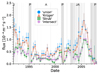 |
Fig. 5. Interstellar dust particle flux for the union (blue circles), Krüger (orange triangles), Strub (green squares), and intersect (violet diamonds) subsets. The data have been aggregated in bins of Δt = 4 months, starting on 1 January 1992, with consideration of the measurement gaps (i.e. the detector dead times), which are indicated by the areas shaded in grey. Horizontal error bars denote the width of the time bin; vertical error bars were calculated as per Appendix B.1.1. Letters at the figure’s top indicate the time of Ulysses’ closest approaches to Jupiter (J), the spacecraft’s perihelia (P), and its aphelia (A). Wall impacts were taken into account for the detector’s sensitivity profile (cf. Fig. B.1), and for the dust kinematics, an inflow direction of (l, b) = (255.41° ,5.03° ) with a speed of vISD, ∞ = 26 km/s was assumed (Swaczyna et al. 2018). (After Janisch 2021, Fig. 5.7.) |
Impacts against the detector’s inner wall can potentially also be measured (cf. Sect. 4.1), which increases the detector’s sensitive surface area (see Fig. B.1; cf. Altobelli et al. 2004). Here, wall impacts were taken into account, rescaling the measured particle flux to lower values (cf. Appendix B.1).
Due to the lower number of events contained in these subsets, the Strub and intersect subsets generally feature much lower fluxes than the other subsets, and the union subset features slightly higher fluxes than the Krüger subset. The magnitude of these differences directly corresponds to the number of events: the union subset contains 1064 events at an average ISD particle flux of 7.4 × 10⁻⁵ m−2 s−1, which is twice as high as the Strub subset with 533 events and an average flux of 3.6 × 10⁻⁵ m−2 s−1. Similarly, the Krüger subset features 952 events with an average flux of 6.6 × 10⁻⁵ m−2 s−1; about ∼10% less than the union subset. At 517 events and an average flux of 3.5 × 10⁻⁵ m−2 s−1 the intersect subset is similar to the Strub subset.
As is evident, the fluxes of all four ISD subsets follow similar general trends. In 1992 the fluxes are roughly twice as high for all four subsets as the respective all-time average flux before decreasing by roughly a third from 1992 until 1995. From 1995 to 2000 all four subsets have low fluxes at roughly half their respective all-time average. In 2000, the fluxes increase to a plateau roughly coincident with the respective all-time average, in 2005 all four subsets feature a notable peak at twice the all-time average, and this is followed by a stark decrease in 2006. The origin of these features is assumed to come from the solar cycle (Strub et al. 2015), as has been corroborated by simulations (Sterken et al. 2015).
The intersect subset typically features the lowest fluxes because it contains the fewest particles. However, at some times, for example in 1994 and from 2005 to 2006, the flux of the intersect subset is higher than the flux of the Strub subset. This is caused by the speed criterion (2.III), which excludes events with low impact speeds from the Strub subset but not from the intersect subset.
There is one notable outlier in mid-1998, where the Krüger subset shows a much higher flux compared to the surrounding time bins (+80%), and the Strub subset does not (−5%). During this time, when Ulysses was at its aphelion and crossed the ecliptic, an excess of low-mass particles was included by the directionality criterion (1.I). This is likely caused by IDPs that were not filtered out by that criterion (Janisch 2021).
In conclusion, Fig. 5 shows that the different ISD selection criteria result in similar global trends of the particle flux but can nevertheless strongly influence local features. This is mostly caused by the lack of small particles in the Strub and intersect subsets, and by the criteria falsely including IDPs or falsely excluding ISD at different times.
5.2. Influence of the ISD selection criteria on the ISD directionality
One of the most salient points of previous analyses of dust impact data from Ulysses is the directionality of the dust impacts (Landgraf 1998; Altobelli 2004; Krüger et al. 2015). The direction of origin of a given dust particle is only known to lie within the opening angle of the dust detector around the detector’s boresight, which is given by the spacecraft rotation angle, ϕrot. The ISD directionality was determined by the average deviation, ϕdev, of the rotation angle at the time the respective particle impacted from the rotation angle of the ISD inflow, ϕISD (Appendix B.2).
Fig. 6 shows the ISD flow directionality (see Strub et al. 2015, Fig. 6) of the impacts of all four ISD subsets. The deviation was averaged within four month intervals beginning on 1 January 1992. Because the Strub and intersect subsets contain fewer particles, the uncertainties of the mean deviation from the ISD rotation angle are higher compared to the other two subsets5.
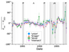 |
Fig. 6. Mean deviation of each events’ rotation angle, ϕrot, from the rotation angle corresponding to the ISD inflow vector, ϕISD, for the union (blue circles), the Krüger (orange triangles), the Strub (green squares), and the intersect (violet diamonds) subsets, averaged over Δt = 4 months beginning on 1 January 1992. Horizontal error bars denote the width of the time bin, and vertical error bars were calculated with Eq. (B.10), taking into account wall impacts (cf. Fig. B.1). Grey-shaded areas and letters at the top edge are as in Fig. 5. (After Janisch 2021, Fig. 5.17.) |
As noted in Sect. 3.2, the Krüger subset mainly selected ISD through its directionality, and it is thus directly biased for this analysis. The mainly mass-based Strub subset is indirectly biased as well. The low-mass particles are expected to have larger deviations due to the Lorentz force, and excluding these particles artificially restricts the ISD directionality.
Until 1999, the average ISD directionality is in reasonably good agreement for the four ISD subsets. The strong deviation of the Strub subset in late 1999 (ϕdev = +63°) from the values at the adjacent times and from the other ISD subsets (ϕdev < 7°) is caused by a single outlier measured at a highly different ϕrot that has a lower quality class; this also occurred in early 19976. Although low-quality outliers are also included in the Krüger subset, its larger number of recorded events is more robust against such outliers7.
The different ISD subsets are not as closely grouped together post-2001 as they were pre-2001. This coincides with the solar maximum that separates the defocusing from the focusing phase of the solar magnetic cycle in 2000–2001. We speculate that the interplanetary magnetic field is least structured close to solar maxima and may chaotically deflect small dust particles. However, the larger deviations, for example in late 2003, are caused by large particles rather than small particles. For this reason, the Strub subset, which lacks the smallest particles and is thus influenced more strongly by large particles, deviates the most by ϕdev = −84°. The Krüger subset, which was filtered by direction and thus does not contain these particles, deviates significantly less by ϕdev = −25° (Janisch 2021).
The most notable feature of this analysis, as remarked by Strub et al. (2015), is the statistically significant change in direction of the dust inflow in 2005–2006, which can be observed in all four ISD subsets. Unfortunately, the following solar minimum in 2008–2009 coincided with the end of measurements, once again highlighting the necessity of long-term measurements of cosmic dust that cover at least a full solar cycle.
5.3. Comparison of the mass determination methods
In this section, we compare the three methods for the determination of the particle mass and impact speed. As a reminder, the measurement-derived speeds and masses were purely derived from the measured signal rise times and amplitudes (Sect. 4.1), the ‘β ≡ 1’ method assumed an identical heliocentric particle speed for all ISD (Sect. 4.2), and the iteratively calculated values assumed heliocentric speeds as per the β-ratios corresponding to the particles’ masses (Sect. 4.3).
In Fig. 7 the impact speeds and particle masses for all events of the union subset are plotted for each method. The measurement-derived values cover a much larger range of speeds and masses. The discrete speed bands of the measurement-derived values stem from the digitisation of the signal rise times into discrete bins. The speed bands with the lowest measurement-derived values, corresponding to vmsr < 3 km/s, contain 34 events with severely underestimated impact speeds and, thus, severely overestimated particle masses (Sect. 4.1). We treat these impact speeds and the corresponding masses as unknown in our analyses unless we explicitly specify otherwise. The lack of high-mass impacts with the ‘β ≡ 1’ method and the iteratively calculated values is directly caused by the lack of low-speed impacts as per Eq. (3): a higher impact speed for a given signal amplitude corresponds to a lower inferred particle mass, and vice versa.
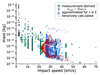 |
Fig. 7. Impact speed and particle mass determined by the measurement-derived method used in the dataset (green circles and black stars), by the approximate method that assumed β ≡ 1 (blue triangles), and by the iterative method (red crosses) using the union subset. The second and third methods assumed an inflow speed of vd = 26 km/s from the direction (lHe, bHe), and the iterative method further utilised the β-curve of adapted astronomical silicates (see Fig. 1). The measurement-derived values for impacts with vmsr < 3 km/s (black stars) most likely feature severely underestimated impact speeds and severely overestimated particle masses. We note that the horizontal axis quantifies the impact speed in the spacecraft frame and not the heliocentric speed. |
All events have the same heliocentric particle speed determined by the ‘β ≡ 1’ method, but their impact speeds vary between ca. 26 km/s and 41 km/s due to the variation of the spacecraft’s heliocentric speed. The distributions of the ‘β ≡ 1’ method and the iterative calculations are more similar because both methods assumed similar heliocentric speeds instead of reconstructing the impact speeds from rise time measurements. The iterative calculations converged to iterative changes below 1% after eight iterations and to below 0.1% after eleven iterations.
The iteratively calculated heliocentric speeds range between 8 km/s < vhel < 38 km/s for the assumed β-curve of adapted astronomical silicates8. These heliocentric speeds were converted to impact speeds in the spacecraft frame for comparison with the measurement-derived impact speeds, which is depicted in Fig. 7. As that figure indicates, the lowest speeds in both the spacecraft frame and the heliocentric frame correspond to those particles with the highest β, which are those with m ≈ 5 × 10⁻¹⁷ kg.
5.4. Influence of the mass determination methods on the ISD mass distribution
The inferred ISD mass distribution is plotted in Fig. 8 for all three determinations of the mass and all four ISD subsets9. The three methods for the determination of the mass agree in their major features: for the Krüger subset the majority of the particles have masses in the range 10−18 kg ≤ m ≤ 10−15 kg, and there is a notable dip in the distribution around m ≈ 10−17 kg that is likely an artefact in the instrument electronics (Grün et al. 1995a). The Strub and the intersect subsets lack the low-mass wing of the distribution, m < 10−17 kg, due to criterion (2.II), and show slightly fewer events in the other bins as well.
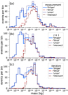 |
Fig. 8. Mass distribution of the Krüger (thick solid blue line), Strub (dashed red line), union (dotted indigo line), and intersect (dash-dotted maroon line) subsets for the masses derived from measurements (panel a; cf. Sect. 4.1), approximated with β ≡ 1 (panel b; cf. Sect. 4.2), and calculated iteratively (panel c; cf. Sect. 4.3) with an assumed density of ρd = 2500 kg/m3. Measurement-derived masses corresponding to vmsr < 3 km/s were not taken into account (cf. Sect. 4.1). (See Krüger et al. 2015, Fig. 5, and Janisch 2021, Fig. 5.32.) |
However, the three mass distributions of the Krüger subset differ in their minor features. For the measurement-derived masses, both flanks of the distribution are much gentler compared to the other two methods. This is a consequence of the assumed heliocentric speeds of the ‘β ≡ 1’ and the iterative method, which constrained the distribution of the impact speeds. The global maximum of the distribution is located at mmsr ≈ 10−15.5 kg for the measurement-derived distribution and the iteratively calculated distribution, and at m = 10−17.5 kg for the ‘β ≡ 1’ method.
Neither the ‘β ≡ 1’ method nor the iterative calculations feature any masses above m > 10−12.5 kg, whereas the measurement-derived distribution does. This is, again, a consequence of the assumed heliocentric speed of the ‘β ≡ 1’ and the iterative method. This upper limit of the ISD mass distribution significantly affects the derived gas-to-dust mass ratio (cf. Sect. 6.4).
The mass distributions of the Krüger subset displayed in Fig. 8 are overall in good agreement with those of Krüger et al. (2015, Fig. 5) but do show some differences: the dip in the distribution at mβ ≡ 1 ≈ 10−17 kg was not resolved by the wider mass bins of Krüger et al. (2015) and may be an instrumental effect. Furthermore, their iteratively calculated mass distribution, which was determined with an assumed dust particle density of ρd = 3300 kg/m3 instead of 2500 kg/m3 as assumed in our analysis, features different heights of its local maxima.
The highest-mass particles of the union subset are separately examined in Sect. 6. Because all mass determinations are heavily dependent on the impact speed of the respective event, highly accurate impact speed measurements would drastically improve the accuracy and precision of any determined mass distribution.
6. Investigating the most massive ISD particles detected by Ulysses
The most massive ISD particles measured by Ulysses are of particular interest: they dominate the differential mass distribution and have the largest effect on the derived gas-to-dust mass ratio of the LISM. Furthermore, because their gyroradii are large, the effect of the heliospheric magnetic field on these particles’ trajectories is negligible compared to the effect of solar gravitation and solar radiation pressure. Thus, the most massive particles are best suited to investigate the particles’ direction of origin (see, e.g., Altobelli et al. 2005).
We compiled two subsets of massive ISD particles based on the union subset: Subset A contains the ten most massive particles, determined by either the measurement-derived or the iteratively calculated masses. Because the measurement-derived masses were most likely severely overestimated for events with impacts speeds below vmsr < 3 km/s, Subset B contains all 45 particles with measurement-derived masses above mmsr > 10−14 kg and impact speeds above vmsr > 3 km/s.
The properties of the particles of Subset A are presented in Sect. 6.1. These particles’ directions of origin is determined in Sect. 6.2. We examine Subset B in Sect. 6.3. Sect. 6.4 reports on the effect of including or excluding particles from Subsets A and B that are unlikely to be interstellar on the inferred gas-to-dust mass ratio in the LISM.
6.1. Properties of the most massive particles of Subset A
We used both the measurement-derived masses, mmsr, and the iteratively calculated masses, miter, to select Subset A. Fig. 9 shows both masses for all particles of the union subset. As expected, there are many particles where mmsr ≈ miter. However, there is also an extended population with mmsr ≫ miter, in particular at high masses.
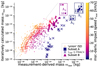 |
Fig. 9. Iteratively calculated mass, miter, versus measurement-derived mass, mmsr, for all particles of the union subset (small circles). The marker colours denote the measurement-derived impact speeds, vmsr. Particles with impact speeds below vmsr ≤ 3 km/s are highlighted as crosses. For these particles, the measurement-derived impact speeds are most likely severely underestimated, and thus the measurement-derived particle masses are severely overestimated (cf. Sect. 4.1). Different clusters of most massive particles, A1, 2, 3, aggregated to Subset A, are highlighted as squares; these particles are numbered 1–10. Another subset of massive particles, Subset B (Sect. 6.3), is marked by triangles. The dotted diagonal line denotes mmsr = miter. |
Most striking in Fig. 9 is a cluster of six particles with mmsr > 10−10 kg, designated as A1 and numbered 1–6. These particles have, by far, the highest measurement-derived masses; however, their iteratively calculated masses are considerably lower at 10−14 kg < miter ≲ 10−13 kg. Another cluster of two particles, designated as A2 and numbered 7–8, features measurement-derived masses that are an order of magnitude lower, 10−11 kg < mmsr ≤ 10−10 kg and even less massive as per the iteratively calculated masses, miter ≈ 4 × 10⁻¹⁵ kg.
These eight particles all feature measurement-derived impact speeds below vmsr ≤ 3 km/s (see Fig. 9), which were most likely severely underestimated (Sect. 4.1). Higher impact speeds would result in lower inferred masses. Thus, the eight particles of A1, 2 are most likely not as massive as assumed10.
For this reason, Subset A also includes the two particles with mmsr > 10−12 kg and vmsr > 3 km/s, designated as A3 and numbered 9–10. These two particles have the highest and the eighth highest iteratively calculated mass, respectively. Their measurement-derived impact speeds are considerably higher, vmsr ≫ 3 km/s.
Properties of the ten particles of Subset A are tabulated in Table 1. There appears to be no pattern to the particles’ heliocentric distances or orbital positions. The iteratively calculated impact speeds are distributed over a wide range of values due to the variation of the spacecraft velocity and of the heliocentric distances at which these particles were detected.
Properties of the particles of Subset A.
The particles of A1, 2 were detected from a wide range of ecliptic longitudes of the detector’s boresight, but appear to be confined to boresight latitudes of −31° ≤bdet ≤ −2°. In contrast, the two particles of A3 were measured while the detector was pointing at fairly high positive latitudes. This disparity may indicate a systematic difference between the particles of A1, 2 and those of A3, for example a different origin of these particles.
6.2. Compatibility of the dust particles of Subset A with an interstellar origin
Different criteria can be used to investigate whether a particular dust particle can be of interstellar origin or not (cf. Sect. 3.2). Sect. 6.2.2 investigates whether the particles’ heliocentric speeds were sufficiently high to correspond to the assumed ISD inflow. This speed criterion only takes into account the (scalar) heliocentric speed of the respective particle, but cannot distinguish between inbound hyperbolic trajectories (i.e. ISD) or outbound hyperbolic trajectories (i.e. β-meteoroids). Therefore, Sect. 6.2.3 investigates whether the directionality of the particles of Subset A agrees with the assumed ISD inflow direction or a Sun-ward origin.
6.2.1. Heliocentric speed of the dust particles
The dust particle properties tabulated in Table 1 are generally insufficient to unambiguously distinguish ISD from IDPs. For example, dust particles from Oort cloud comets (OCCs) often have large eccentricities and come from all longitudes, including the direction of the ISD inflow (Poppe 2016). However, the orbits of OCCs, and thus the orbits of the majority of the dust particles originating from OCCs, are elliptic11, whereas the orbits of ISD particles are hyperbolic. Thus, the local heliocentric speed of an OCC dust particle must be lower than the local escape speed, which is
 (5)
(5)
whereas the speed of an ISD particle is generally higher as per Eq. (4). We note that the Lorentz force is not taken into account here. While it does not play a significant role for these most massive particles due to their large gyroradii, it cannot be ignored for lower-mass particles.
The heliocentric speed, vhel, of a dust particle encountered by Ulysses is not known; only the particle’s impact speed, vmsr, could be determined from the detector signal (cf. Sect. 4.1). This value has a multiplicative error factor of 1.9 (Grün et al. 2010); the true value of the impact speed lies within the interval [vmsr/1.9; vmsr ⋅ 1.9].
Therefore, the particle’s heliocentric speed must be reconstructed from the particle’s and the spacecraft’s orbital velocities. However, the relative direction from which an impacting particle came is only known to have lain within the detector’s field of view, limiting how precisely the particle’s heliocentric speed can be reconstructed. Thus, the detector’s opening angle of 70° introduces an additional maximum error factor of the heliocentric speed of up to 1.36 at Ulysses’ aphelion and up to 3.8 at its perihelion (cf. Appendix C). For the configuration of Ulysses we assume that these error factors are roughly multiplicative12. Therefore, assuming an opening angle of 70°, the heliocentric speeds could only be reconstructed with a total error factor between 1.9 ⋅ 1.36 ≈ 2.6 at the aphelion and 1.9 ⋅ 3.8 ≈ 7.2 at the perihelion.
To unambiguously distinguish ISD from dust on elliptic orbits, the heliocentric speed must be known with an error factor smaller than 1.73 at the heliocentric distance of Jupiter (cf. Appendix C). At 1 au the required precision is even finer with an error factor smaller than 1.18. To distinguish ISD from dust on circular orbits, these precision limits increase to 2.44 for Jupiter and 1.66 for Earth. The configuration of the dust detector on board Ulysses does not meet these requirements; in many cases ISD cannot be distinguished from OCC dust.
6.2.2. Compatibility of the particles’ heliocentric speed with ISD
Table 2 lists the most likely reconstructed heliocentric speed, vrec, hel, for the particles of Subset A, using Eq. (C.1). The same table also gives confidence intervals, taking into account either only a finite opening angle of 70°, or both that finite opening angle and the error factor of the impact speed determination. For convenience, the heliocentric speed of Ulysses, as well as the heliocentric speeds of a particle on a circular orbit, on a parabolic orbit (i.e. the escape speed) according to Eq. (5), and for an ISD particle on a hyperbolic orbit according to Eq. (4) are tabulated as well, taking into account the β-ratio corresponding to either the measurement-derived or the iteratively calculated particle mass. We based the reconstruction of the most likely heliocentric speed on the measurement-derived impact speed, vmsr, only if vmsr > 3 km/s. Otherwise, the iteratively calculated relative speed, viter, was used. However, because the iterative calculation assumes that the particles are ISD, the resulting speeds cannot be used to confirm an ISD origin but can only reject this hypothesis should the resulting speeds be inconsistent with the local hyperbolic ISD speed.
Measurement-derived impact speeds, vmsr > 3 km/s, were only available for the particles of Subset A3. For particle (9) the most likely reconstructed heliocentric speed, vrec, hel ≈ 19.0 km/s, is slightly higher than the local escape speed, vesc ≈ 17.9 km/s, but considerably lower than the local hyperbolic ISD speed, vhel, ISD = 31.5 km/s. For particle (10), the local escape speed is higher than the reconstructed heliocentric speed, indicating that this particle is unlikely to be ISD.
Although the iterative calculation of the relative speed, viter, assumes that the particles of Subsets A1, 2 are ISD, the resulting most likely heliocentric speeds are lower than the local escape speed for particle (1) and considerably lower than the local hyperbolic ISD speed for particles (1–3), (5), and (8), contradicting the assumption of an ISD origin. Only for particles (4) and (6–7) the most likely reconstructed heliocentric speeds are faster than the hyperbolic ISD speed.
When taking into account the uncertainties of the reconstructed heliocentric speed introduced by the opening angle of the detector and the error factor of the measurement-derived impact speed, the resulting ranges of reconstructed heliocentric speeds typically include both the local escape speed and the local hyperbolic ISD speed. The exceptions are particles (9–10), which may have been faster than the respective local escape speed but do not agree with the speed of a hyperbolic ISD particle. It is thus unlikely that particles (9–10) are ISD, although they may have come from interstellar objects other than the LISM.
Because the iteratively calculated impact speeds are based on the assumption of ISD, this analysis can only reject the hypothesis that a particle is ISD if the resulting speeds are inconsistent with this underlying assumption, but it cannot confirm whether particles (1–8) are ISD due to circular reasoning. Only for particles (4) and (6–7) the most likely reconstructed heliocentric speeds are consistent with the basic assumption of ISD. For the other fives particles of A1, 2 the analysis is inconclusive due to the large uncertainty introduced by the wide opening angle of the detector.
We note that the Strub subset does not contain these ten massive particles because criterion (2.III) excluded all particles with impact speeds below vmsr < 13 km/s. As mentioned in Sect. 6.2.3, seven of these ten particles agree with the ISD inflow direction as per criterion (I.1), taking into account an opening angle of 90° around the detector’s boresight.
This analysis demonstrates that more precise measurements of the impact speed and particle directionality would enable the identification of ISD by the particles’ reconstructed heliocentric speeds. We estimate that the total error factor of the reconstructed heliocentric speed must lie below 1.73 to distinguish ISD from highly eccentric IDPs on spacecraft with Jupiter-like orbits (cf. Appendix C). For spacecraft on Earth-like orbits, the total error factor shrinks to 1.1813.
6.2.3. Compatibility of the particles’ direction with ISD
Fig. 10 shows the orbital position of Ulysses as well as the detector boresight at the time of impact for each particle of Subset A. Coloured areas indicate the outer edge of the cone of view corresponding to an opening angle of the detector of ±70°, meaning that wall impacts were not considered (cf. Appendix B.1). If wall impacts are considered, the opening angle is ±90°, meaning that the full hemisphere centred around the boresight would be sensitive to impacts. However, close to the outer edge of the cone of view, the effective sensitive surface area is almost zero. Therefore, it is far more likely that a particle came from closer to the boresight direction than from a direction close to the outer edge of the cone of the view.
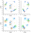 |
Fig. 10. Ulysses’ orbital position and the detector’s boresight and cone of view at the times of the most massive particle impacts in the ecliptic xz- (left) and yz-plane (right). The detector boresight and its cone of view were Galilean-transformed from the spacecraft frame to the heliocentric frame, which distorts the cones of view. The Galilean transformation assumes that the dust particles’ relative velocity corresponds to the inverse boresight direction and either the measurement-derived impact speeds, vmsr (top), or the iteratively calculated impact speeds, viter (bottom). The ISD inflow is marked by grey arrows (see Fig. 3). The orbital positions at which the particles of Subset A impacted are indicated by blue squares, red triangles, and green circles for A1, 2, 3, respectively. The black lines point in the detector boresight, scaled identically in both panels. The coloured areas give the outer edge of the cone of view with an opening angle of ±70°, corresponding to the detector’s sensitivity without considering wall impacts. We note that the measurement-derived impact speeds are most likely spurious for the particles of A1, 2, and that the iteratively calculated relative speeds assume an ISD origin. Particles are numbered as in Fig. 9. The deviation of the boresight from the ISD inflow direction is tabulated in Table 2. |
The detector’s field of view takes the shape of a rotationally symmetric cone with an opening angle of 70° around the boresight (see Table 1) in the spacecraft’s frame of rest. However, because Ulysses and its dust detector were in motion with respect to the heliocentric reference frame, both the detector’s boresight and its field of view will appear geometrically distorted in the heliocentric reference frame. This was accounted for by a Galilean transformation from the spacecraft’s frame of rest to the heliocentric reference frame14,
 (6)
(6)
where  is the detector boresight or a generatrix15 of its cone of view; vi is the relative speed of the particle in the spacecraft’s frame of rest, which is assumed to be either the measurement-derived impact speed, vmsr, or the iteratively calculated impact speed, viter; their product,
  , is the assumed dust particle velocity in the spacecraft’s frame of rest, which is subtracted from the heliocentric spacecraft velocity, vU. This Galilean transformation results in the boresights and cones of view shown in Fig. 10.
The angles of deviation of the ISD inflow direction from the detector boresight are tabulated for all ten particles of Subset A in Table 2. Seven of these ten particles are part of the Krüger subset; they were measured when the detector’s boresight was within ±90° of the assumed ISD inflow direction, that is, under consideration of wall impacts. Nevertheless, due to the Galilean transformation, some of these particles lie close to the outermost edge or even outside of the detector’s cone of view when taking the spacecraft velocity into account. When assuming that the particles impacted with the measurement-derived impact speed, all ten particles of Subset A were measured when the ISD inflow direction lay outside the 70°-cone of view. However, the measurement-derived impact speeds are most likely spurious for all particles of Subsets A1, 2. When using the iterative calculation of the impact speed, which assumes that the respective particle is ISD, the ISD inflow direction lay within the 70°-cone of view for only four of the ten particles: (3), (5), (8), and (10)16. For three of these four particles the ISD inflow direction lay close to the outer edge of the cone of view,  . This is in agreement with the reconstructed heliocentric speeds, which are not consistent with the local hyperbolic ISD speeds for
  but are consistent for
  (Sect. 6.2.2). Nevertheless, the detector’s sensitive surface area decreases with increasing impact angle (Fig. B.1). For any given impact, it is less likely that the particle came from close to the outer edge of the detector’s cone of view.
This indicates that three to four of the ten massive particles of Subset A may have been ISD but we cannot confirm it. The other six to seven massive particles may have come from cometary streams (Krüger et al. 2024a) or may have been more sporadic IDPs. More precise information on the particles’ direction of origin would be invaluable to more accurately distinguish ISD from IDPs.
This analysis can also be applied to other directions of origin: four of the ten particles of Subset A – including all ISD candidates – agree with a Sun-ward direction of origin even without considering wall impacts, indicating that they could be β-meteoroids (e.g. Wehry et al. 2004). However, these particles would be unusually massive for β-meteoroids.
6.3. Compatibility of the not-as-massive particles of Subset B with an interstellar origin
Infrared observations of the ISM and considerations of its elemental abundances suggest that ISD particles with masses of m > 10−12 kg are unexpected (Draine 2009), which is consistent with the indication that the measurement-derived particle masses for Subsets A1, 2 are most likely severely overestimated. Another caveat of the mass determination is that the instrument calibrations that derive the impact speeds from the signal rise times and the masses from the signal amplitudes (Sect. 4.1) all assume compact dust particles. Recent laboratory experiments have shown that porous (‘fluffy’) particles would yield different calibration curves depending on the densities of the dust particles and the impact target: a miscalibration may result in incorrect impact speeds and masses (Hunziker et al. 2022). Combining these considerations, it is expedient to not only investigate the particles of Subset A, but to also examine particles of lower but still reasonably high masses that also have reasonably high impact speeds, compiled as Subset B.
This subset of events was selected with an arbitrary lower mass threshold of mmsr > 10−14 kg, corresponding to particle radii of a ≳ 1 μm17. All particles with a measurement-derived impact speed below vmsr < 3 km/s (cf. Fig. 9) were excluded because the corresponding measurement-derived masses are most likely severely overestimated. Subset A3 was removed as well because we have already scrutinised it in detail in the previous section. The resulting subset consists of 45 particles with masses within 10−14 kg ≤ mmsr ≤ 10−12 kg and 10−16 kg ≤ miter ≤ 10−14 kg, and one particle with vmsr = 3.4 km/s and miter = 3.38 × 10⁻¹⁷ that was removed due to its comparably low iteratively calculated mass. The resulting Subset B is marked in Fig. 9. The particles’ properties and their reconstructed heliocentric speeds are tabulated in Tables E.1 and E.2, respectively.
Not a single particle of Subset B has a most likely reconstructed heliocentric speed, vrec, hel, that is at least as fast as the local hyperbolic ISD speed, vhel, ISD. However, one particle, numbered #31 in Table E.2, falls short by only 1%; the ISD inflow direction also deviates by less than  from the detector boresight at the time particle #31 impacted. If the total error factors of the heliocentric speed reconstruction are taken into account, 20 of 45 particles both have reconstructed heliocentric speeds that come within 10% of the respective local hyperbolic ISD speed and agree with the ISD inflow direction. Relaxing the directionality criterion to ±90° increases this number further to 30 ISD candidates18.
Of the 45 particles of Subset B only eight both agree with the ISD inflow direction within 70° and are faster than the local escape speed, Eq. (5), without accounting for the total error factors of the reconstruction of the heliocentric speed. Taking both the total error factors and wall impacts into account increases the number of potentially interstellar particles to 4119. The remaining four particles agree with the speed criterion but not with the directionality criterion.
To summarise, for only one of the 45 particles within the mass range 10−14 kg ≤ mmsr ≤ 10−12 kg and with impact speeds vmsr > 3 km/s an interstellar origin can be ascertained, and for only four of those particles it can be ruled out. As a rough estimate, one may assume that between a quarter and two thirds of the particles of Subset B may be interstellar.
6.4. Local interstellar gas-to-dust mass ratio
The gas-to-dust mass ratio in the LISM, Rg/d, is calculated by dividing the mass density, ρgas, of gas in the VLISM by the mass density, ρISD, of the ISD measured by Ulysses:
 (7)
(7)
Details on how to calculate the gas mass density and the dust mass density are given in Appendix B.3. Here we assume a gas mass density of ρgas ≈ 5.14 × 10⁻²² kg/m3 (Krüger et al. 2015). The resulting gas-to-dust mass ratio will be slightly inaccurate because it does not take the filtering of ISD by the heliosheath into account (cf. Sect. 7.6): the mass distribution of ISD in the Solar System, where it can be measured in situ by, for example, Ulysses, is not expected to be identical to the pristine mass distribution of ISD in the LISM. However, massive particles, which contribute most strongly to the dust mass density, are the least affected by the filtering in the heliosheath (cf. Sect. 7).
Taking into account the measurement-derived masses of all particles of the Krüger subset, including those with vmsr < 3 km/s that most likely feature severely overestimates masses, results in an unrealistically low gas-to-dust mass ratio of  (see Table 3). If the particles with vmsr < 3 km/s are excluded, the gas-to-dust mass ratio increases by more than two orders of magnitude to
  . For comparison, Slavin & Frisch (2008) estimate a hydrogen gas-to-dust mass ratio of Rg/d ∈ [149, 217] over the ∼130 pc-long sightline to ε CMa.
Interstellar dust mass density and gas-to-dust mass ratio in the LISM.
The comparably low value we determined stems from the influence of the most massive particles. As Sects. 6.2 and 6.3 show, many (if not most) of these particles are likely not of interstellar origin and should thus be excluded from the ISD mass distribution. Excluding all particles with measurement-derived masses above mmsr ≥ 10−12 kg in accordance to the investigation into Subset A (see Sect. 6.2), and further removing an arbitrary half of all particles with measurement-derived masses above mmsr ≥ 10−14 kg in accordance to the investigation into Subset B (see Sect. 6.3) yields higher gas-to-dust mass ratios that are tabulated in Table 3. The inclusion of the possible ISD candidates of Subset A, particles (3, 5, 8, 10), severely influences the gas-to-dust mass ratio. For example, particle (10) by itself, which is the only ISD candidate of Subset A for which the measurement-derived mass, mmsr = 3.69 × 10⁻¹² kg, is not spurious, decreases the gas-to-dust mass ratio from  to
to  if it is included.
If, as was done by Krüger et al. (2015), the iteratively calculated masses are used instead of the measurement-derived ones, the gas-to-dust mass ratio is considerably higher. Assuming that the majority of the particles of Subset A and about half the particles of Subset B are not interstellar, it is reasonable to remove an arbitrary half of all particles with iteratively calculated masses above miter ≥ 10−15 kg. The resulting dust mass densities and gas-to-dust mass ratios are tabulated in Table 3. Using the iteratively calculated masses, the gas-to-dust mass ratio that corresponds to the most likely selection of ISD – including only the ISD candidates of Subset A and excluding half of Subset B – is  .
.
This gas-to-dust mass ratio is significantly affected by the inclusion or exclusion of even a single massive ISD candidate. Excluding particle (5), which has an iteratively calculated mass of miter = 1.07 × 10⁻¹³, increases the gas-to-dust mass ratio from  to
to  . This, as well as the large spread of the determined gas-to-dust mass ratios over more than one order of magnitude, shows how essential it is to be able to determine the origin and particle mass of the impacting dust particles with high accuracy. A more definitive selection of ISD particles would yield a more definitive gas-to-dust mass ratio. If the impact speeds were known with higher precision, the error factor of the determined masses and the uncertainty of the resulting gas-to-dust mass ratio could be reduced.
These gas-to-dust mass ratios are determined from the gas density in the VLISM and the dust density in the inner heliosphere. A correction for the modulation and filtering processes of ISD in the heliosheath (Sect. 7) would be required to more accurately determine the gas-to-dust mass ratio in the VLISM. However, these filtering effects are expected to act most severely on low-mass particles, which do not influence the gas-to-dust mass ratio as strongly as high-mass particles.
7. Investigating the filtering of interstellar dust in the heliosheath
Numerical simulations of ISD impacts on Ulysses were performed by Sterken et al. (2015). Their model did not include the heliosheath and could reproduce the measurements made by Ulysses either before or after ca. 2003 but not over the entire time span from 1992 to 2008. Sterken et al. (2015) ascribed this to a time-dependent filtering of ISD in the heliosheath, which is assumed to vary with the solar magnetic cycle through the Lorentz force.
By comparing numerical simulations similar to those by Sterken et al. (2015) to the measurements made by Ulysses, the time-dependent filtering function of ISD in the heliosheath can be constrained. The resulting heliosheath filtering function can then be applied to other spacecraft, allowing for more precise predictions of the encountered particle fluxes and measured size distributions of these other missions (see, e.g. Hunziker et al., in prep., for an application to DESTINY+).
7.1. Modulation of the LISM interstellar dust size distribution
As ISD moves from its unfiltered origin in the LISM, it experiences three general phenomena that can modulate its size distribution:
-
As ISD enters the heliosphere, it is filtered by the heliosheath through the Lorentz force, which varies with the solar magnetic cycle (see Table 4)20. The exact details of this filtering are unknown but assumed to predominantly depend on particle properties such as the dust size, composition, and porosity. According to simulations, small particles (a ≲ 0.03 μm) cannot enter the heliosphere, with the exact cutoff size depending on the phase of the solar cycle (Slavin et al. 2012).
Table 4.Minima and maxima of the solar magnetic cycle during the Ulysses mission.
-
On their trajectory from the heliopause to the detector ISD particles are affected by solar gravitation, solar radiation pressure, and the Lorentz force, the latter of which is highly dependent on the phase of the solar cycle, the particle size, composition, and porosity (‘fluffiness’).
-
What is measured by the detector depends, in addition to the ISD flux, on the effective sensitive surface area of the detector with respect to the ISD flow and on the relative speed between the dust particle and the spacecraft (cf. Appendix B.1); this is time-variable and size-dependent as well.
Assuming an, at this point, unspecified differential size distribution of ISD in the ISM, (dn/da)ISM, the differential size distribution that is measured by Ulysses at a given time of observation can be described by
 (8)
(8)
where fhs is the filtering function of the heliosheath, fF describes the modulation of the size distribution by the forces in the inner heliosphere, and fdet is the detector transfer function.
While the exact nature of the heliosheath filtering, fhs, is unknown, the modulation by forces in the inner heliosphere, fF, has been well investigated with numerical simulations (Sect. 7.3), and the detector transfer function, fdet, can be semi-analytically calculated (Sect. 7.4). Therefore, the heliosheath filtering function can be retrieved by (see Hunziker et al., in prep.)
 (9)
(9)
where (dn/da)obs is derived from spacecraft measurements, and (dn/da)ISM must either be assumed or derived from remote astronomical observations. We term  the inferred size distribution at the termination shock (cf. Sect. 7.5).
7.2. Measured size distribution of interstellar dust
The measurement-derived differential size distribution of the union subset in finite size bins, (Δn/Δa)obs, as detailed in Appendix D.1, is plotted in Fig. 11a. For comparison, the extended MRN distribution (Mathis et al. 1977),
 (10)
(10)
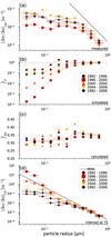 |
Fig. 11. Measurement-derived differential size distribution, (Δn/Δa)obs (panel a); time-averaged modulation factor through forces in the Solar System, |


has been graphed as well, where Ci is a normalisation constant, CC = 10−25.13 cm5/2/H for carbonaceous grains and CSiO = 10−25.11 cm5/2/H for silicates (Draine & Lee 1984). The MRN distribution, which is valid only up to particle sizes of 0.25 μm for silicates and 1 μm for carbonaceous grains, has been extended over the entire particle size range of the available simulations, summing the distributions for silicates and carbonaceous grains, Ci = CC + CSiO. The number density of hydrogen nuclei, nH = 0.1 cm−3, is uncertain; the resulting MRN distribution could be shifted to higher or lower values. We note that the MRN distribution has been derived from remote astronomical observations over long lines of sight through the Galaxy, assuming that the dust types and size distribution are similar in the LIC.
The measured differential size distribution has been plotted in Fig. 11a for four four-year subsets of the data to illustrate the influence of the solar cycle, and additionally for all sixteen years of measurements. In the determination of the length of the four-year time bins, the measurement gaps such as perihelion crossings, dust stream crossings, or instrument switch-offs have been taken into account; vd = 26 km/s has been assumed throughout.
As is expected, the measured differential size distribution is reduced compared to the assumed MRN distribution and deviates more strongly for smaller particles than for larger ones. In the time period of 1996–2000, immediately following the solar minimum of the defocusing phase in August 1996 (cf. Table 4), the measured differential size distribution is strongly reduced compared to the MRN distribution, especially at small particle sizes, because fewer ISD particles were detected (Landgraf 2000; Sterken et al. 2012a)21. Conversely, in the time period of 2004–2008, preceding the solar minimum of the focusing phase in November 2008, the measured differential size distribution is considerably higher, especially for intermediate particles (a ≈ 0.1 μm).
The vertical error bars in Fig. 11a stem from the standard deviation of the number of measured particle impacts per size and time bin, Eq. (D.5). These errors are largest for the time period following the solar minimum of the defocusing phase, 1996–2000, during which the fewest particles were recorded. In order to avoid low statistics, it is inadvisable to divide the data into too many time intervals; therefore, no finer time resolution was chosen. Further uncertainties are discussed in Sect. 7.7.
7.3. Size-dependent, time-averaged modulation of interstellar dust by forces in the inner heliosphere
The modulation factor through the forces in the Solar System, fF, has been investigated by numerical simulations of dust particle trajectories with the IMEX code (Sterken et al. 2012a; Strub et al. 2019). This code returns the time-dependent factor by which the number density, n, of ISD at a given particle size, a, is enhanced or reduced compared to a reference density, nISM, due to solar gravitation, solar radiation pressure, and the Lorentz force in the inner heliosphere:
 (11)
(11)
More details on the simulations are provided in Appendix D.2.
Fig. 11b shows the size-dependent, time-averaged modulation factor,  , for the same four time periods as the measured differential size distribution; the time-dependent modulation is given in Appendix D.3. As Fig. 11b shows, the simulated modulation factor through the forces in the Solar System at the location of Ulysses approaches fF ≈ 1 for large particles, and drops for smaller particles (fF < 1). However, in the time period preceding the solar minimum of the defocusing phase (1996), particles of intermediate size (0.15 μm < a < 0.5 μm) were enhanced at Ulysses’ orbit.
7.4. Size-dependent, time-averaged detector transfer function
The effective sensitive surface area of Ulysses’ dust detector depends on the angle of incidence, α, between the detector’s boresight and the direction from which the dust particles came, and on the relative speed, |vrel|, between the dust and the spacecraft. In analogy to Appendix B.1, the time-dependent and size-dependent detector transfer function is given by
 (12)
(12)
where Asens(α) is the angle-of-incidence-dependent sensitive surface area of the detector (see Fig. B.1), Amax = 0.1 m2 is the detector’s total surface area, and vrel(a;t) has been taken from the numerical simulations. This detector transfer function, fdet, indicates how strongly the measured particle flux appears enhanced or reduced compared to the particle flux at the spacecraft’s orbital position.
The time-averaged detector transfer function,  , has been averaged over the same time periods as
  ; it is plotted in Fig. 11c. The time-dependent detector transfer function is shown in Appendix D.4.
The accuracy of this transfer function is limited by the averaging of the simulated particles within each simulation grid cell. However, because the transfer function remains within  , the influence of its variation is not as strong as that of fF, which changes by multiple orders of magnitude. Further uncertainties are discussed in Sect. 7.7.
7.5. Inferred size distribution of interstellar dust at the termination shock
The differential size distribution at the outer border of the inner heliosphere, the termination shock, was inferred by applying the inverse of  and
and  to the measured differential size distribution, Eq. (9). This is plotted in Fig. 11d together with the MRN distribution, Eq. (10).
As Fig. 11d shows, the shapes of the inferred differential size distributions fit reasonably well to the MRN distribution for intermediate and large particles but deviate more strongly from a MRN-like power law for small particles. In the time period of 1992–1996 that precedes the solar minimum of the defocusing phase of 1996 (cf. Table 4), the inferred number density for small particles is lowest, whereas in the next time period, 1996–2000, immediately following this solar minimum, it is highest. This is a notable difference from the measured differential size distribution, where the opposite holds, and stems from the modulation factor due to inner heliosphere forces in relation to the measurements,  , which causes the weakest depletion during 1992–1996 and the strongest depletion during 1996–2000 (see also Sterken et al. 2015).
The inferred differential size distribution agrees with the findings of Slavin et al. (2012), who found a strong depletion of small particles (a ≲ 0.1 μm) at the outer boundary of the inner heliosphere during the defocusing phase, and an enhancement locally at the heliosheath during the focusing phase.
The vertical error bars graphed in Fig. 11d correspond to the Gauss-propagated standard deviations of the measured size distribution, Eq. (D.7). Further uncertainties of this analysis are discussed in Sect. 7.7.
7.6. Filtering modulation of ISD in the heliosheath
The resulting time-averaged heliosheath filtering function,  , Eq. (9), is calculated by dividing the inferred differential size distribution (Fig. 11d) by the MRN distribution, Eq. (10). Fig. 12a shows the heliosheath filtering function versus the particle size for the previously used four-year time periods. The vertical error bars correspond to the vertical error bars of the inferred differential size distribution, Eq. (D.9), which take into account only the (assumed) Poissonian standard deviation of the number of measured particle impacts per size and time bin. We discuss additional uncertainties in Sect. 7.7.
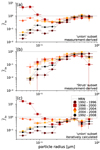 |
Fig. 12. Heliosheath filtering function, Eq. (9), in relation to the particle size, for the same time periods as Fig. 11, for the union subset with measurement-derived masses (panel a), for the Strub subset with measurement-derived masses (panel b), and for the union subset with iteratively calculated masses (panel c). The vertical error bars correspond to the (assumed) Poissonian standard deviation of the number of particles within the respective size and time bin (cf. Appendix D.5), (see Hunziker et al., in prep.). |
As expected,  for large particles (a > 0.4 μm), and
  for intermediate and smaller particles, except in the time period that immediately follows the solar minimum of the defocusing phase, 1996–2000 (cf. Table 4), where
  . This may be caused by the filtering modulation through inner heliosphere forces in the simulations, fF, which reduces the number of small particles during this time period more strongly by at least an order of magnitude compared to other time periods (cf. Fig. 11b), in comparison with less filtering in the Ulysses dataset. This may indicate a focusing effect for small particles in the heliosheath during 1996–2000.
ISD particles measured by Ulysses in 1996–2000, which experienced a strong defocusing phase inside the Solar System, would have crossed the termination shock in ca. 1981–198522. This time period coincides with the focusing phase surrounding the solar minimum of 1986, comparable to the time period of 2004–2008 preceding the solar minimum in 2008/2009, one ∼22 yr-cycle later. A similar focusing effect of ISD in the heliosheath has been simulated by Slavin et al. (2012) using a static focusing heliospheric magnetic field in the entire heliosphere including the heliosheath. This was illustrated by Sterken et al. (2015, Fig. 19) and later simulated by Godenko & Izmodenov (2024).
We note that the total travel time of ISD from the LISM to the inner Solar System is approximately 20–22 yr23, which is comparable to the period of the solar magnetic cycle (Sterken et al. 2015). The width of the heliosheath varies over the solar magnetic cycle (Scherer & Fahr 2003). Thus, the time ISD spends in the heliosheath may vary with the phase of the solar magnetic cycle as well (see, e.g., Sterken et al. 2015, Fig. 19).
The time-averaged heliosheath filtering function that spans the full time range, 1992–2008, strongly resembles  for the time period preceding the solar minimum of the defocusing phase, 1992–1996. Nevertheless, that
  deviates from its average so strongly for the time periods of 1996–2000 and 2000–2004 shows how important it is to treat this analysis in relation to the phase of the solar cycle. For a more accurate assessment, it would be essential to apply this methodology to a larger dataset that spans a full solar magnetic cycle or, ideally, even multiple cycles24.
7.7. Uncertainties of the heliosheath filtering modulation
Due to its complexity and the large number of assumptions, the analysis illustrated in the previous sections has multiple sources of uncertainty.
In Figs. 11 and 12 the vertical error bars only correspond to the Poissonian standard deviation of the number of particle impacts per size and time bin (see Appendix D.5). There are, however, more uncertainties and assumptions that are not taken into account, such as the error factor of the measurement-derived particle mass, which is typically an order of magnitude (Grün et al. 1995a).
As Figs. D.2 and D.3 show, the time-dependent modulation by inner heliosphere forces, fF, and the time-dependent detector transfer function, fdet, are not constant during the selected time intervals. Time-averaging these functions introduces uncertainties that are not taken into account by the error bars of Figs. 11 and 12. Smaller time intervals would reduce these uncertainties and result in a finer time resolution of the heliosheath filtering function25. However, dividing the total number of particles into more bins would require a larger dataset. This also holds true for the bin width of the particle size.
Further uncertainties lie in the nature of the numerical model, for example via the assumption for the interplanetary magnetic field (see, e.g. Sterken et al. 2012a). Furthermore, in each model cell, the particle velocity is averaged over all particles, introducing another uncertainty. Yet another uncertainty stems from the assumed β-curve; if a different β-curve were assumed, different parameter sets of the numerical model, (β, Q/m), would have to be used. Succinctly put, the heliosheath filtering modulation derived by this method is only as good as the numerical model. Finally, uncertainties of the MRN distribution, including a possible deviation from the MRN distribution by the ISD size distribution in the LISM, are not taken into account in our analysis.
The choice of the ISD selection criteria (cf. Sect. 3.2) and the mass determination method (cf. Sect. 4) have an influence as well. This is investigated in Sects. 7.7.1 and 7.7.2, respectively.
7.7.1. Uncertainties introduced by the choice of the ISD selection criteria
The above analysis was performed with the union subset. For the Krüger subset, which lacks some of the particles in the intermediate-to-large size range but is otherwise similar to the union dataset (see Fig. 8), the inferred differential size distribution changes only negligibly.
For the Strub subset, low masses have been excluded; thus, no data is available for the lowest size bin, and the lower end of the differential size distribution is depleted more strongly. This is shown in Fig. 12b. The Strub subset contains only half as many events as the union subset. The resulting differential size distributions, and therefore the heliosheath filtering function also shows values that are lower by roughly a factor of two. However, the exclusion of low-mass particles in the Strub subset directly biases the ISD size distribution much more strongly than the indirectly biased Krüger subset does; the Strub subset was not devised to investigate the ISD mass or size distribution (Strub et al. 2015). Therefore, it is not advised to use the Strub subset for this type of analysis; here, we have used it merely for comparison with the other datasets.
7.7.2. Uncertainties introduced by the choice of the mass determination method
So far, the masses as derived from the measured signal rise times and amplitudes were used to calculate the particle sizes (cf. Sect. 4.1). If, instead, the approximate determination of the mass (‘β ≡ 1’, cf. Sect. 4.2) is used, the inferred differential size distribution shows only minor differences (not depicted).
If the iterative method (cf. Sect. 4.3) is used to determine the particle masses, the resulting inferred differential size distribution is also remarkably similar to the distributions generated with the masses of the other mass determination methods. This is shown by Fig. 12c. Nevertheless, some differences are apparent: large particles (a ≈ 0.54 μm) are depleted more strongly by half an order of magnitude for the iterative method compared to the measurement-derived mass determination, notably deviating from the extended MRN distribution even when accounting for statistical uncertainties. For small particles (a < 0.15 μm) the heliosheath filtering factor deviates by less than half an order of magnitude from the results for the measurement-derived mass determination, and at intermediate sizes the results are only negligibly dependent on the mass determination method. This holds true for all observed time periods.
8. Summary and conclusions
We have performed three distinct analyses of the dataset of ISD impacts on the Ulysses spacecraft. We investigated the influence of the choice of the different ISD selection criteria and of the competing mass determination methods on the ISD particle fluxes, directionality, and mass distribution (Sect. 5). We scrutinised the most massive particles detected by Ulysses to determine whether they are ISD, which affects the gas-to-dust mass ratio in the LISM inferred from in situ measurements (Sect. 6). We backcalculated the filtering effect of ISD in the heliosheath from the ISD size distribution measured by Ulysses with the aid of numerical simulations (Sect. 7). The resulting filtering modulation can be used to predict the fluxes on other spacecraft in the Solar System, including the effect of the heliosheath filtering without the need for a full heliosphere simulation (cf. Hunziker et al., in prep.). These investigations are summarised in Sect. 8.1, 8.2, and 8.3, respectively.
8.1. Conclusions of the investigation into the ISD selection criteria and mass determination methods
The influence of the different ISD selection criteria on the ISD particle flux and the ISD flow direction was investigated in Sects. 5.1 and 5.2. We make the following conclusions.
The different ISD selection criteria bias the resulting ISD subsets in different ways by design (Krüger et al. 2015; Strub et al. 2015). For example, the criterion that identifies ISD by its direction, (1.I), was devised by Krüger et al. (2015) to investigate the particles’ mass distribution, and it directly biases the directionality of the resulting Krüger subset. The criterion that excludes IDPs based on the measured signal amplitudes, (2.II), was devised by Strub et al. (2015) to investigate the particles’ directionality, and it directly biases the mass distribution of the resulting Strub subset. Nevertheless, criterion (1.I) also indirectly biases the mass distribution, and criterion (2.II) indirectly biases the directionality of the respective subsets.
The different criteria for ISD identification do not result in different long-term patterns in the particle flux or flow direction, except for a general factor of approximately two of the particle flux between the Krüger and the Strub subsets that directly stems from the number of particles contained in the respective subset. However, the different criteria do influence local features. This is, in most cases, caused by the lack of small particles in the Strub subset. For example, the Strub subset contains ∼44% fewer impacts than the Krüger subset, and the resulting particle flux is systematically lower by ∼45%. The shift in the ISD directionality in 2005–2006 is observed for all ISD subsets.
The most massive ISD particles measured by Ulysses dominate the differential mass distribution and have the largest influence on the gas-to-dust-mass ratio. Therefore, we compared the three different mass determination methods in Sect. 5.3 and the resulting mass distributions in Sect. 5.4. We came to the following conclusions.
The overall shape of the resulting mass distribution is similar for all three mass determination methods except that neither the mass distribution of the ‘β ≡ 1’ method nor of the iterative calculations feature any masses above m > 10−12.5 kg, whereas the measurement-derived distribution does, thus confirming earlier results by Landgraf (1998) and Krüger et al. (2015). The distribution of the measurement-derived impact speeds covers a much wider range than for the other methods. The iterative method assumes an interstellar origin and thus cannot be used to determine whether a given particle is interstellar or not. The iterative method is generally flawed, as it does not take into account the directionality of the respective particle. This does not only pertain to the effects of the Lorentz force but also the deflection by solar gravitation and solar radiation pressure. We furthermore note that the inferred gas-to-dust mass ratio in the LISM (Sect. 6.4) is higher by orders of magnitude when using the iteratively calculated masses than when using the measurement-derived masses (see also Sect. 8.2).
8.2. Conclusions of the investigation into the most massive ISD particles detected by Ulysses
We investigated the most likely origin of the ten most massive ISD particles detected by Ulysses in Sect. 6.2 and conclude the following. Three to four of these ten particles may be compatible with the particle speed and direction of the ISD inflow. However, due to large measurement uncertainties, these particles cannot be unambiguously identified as ISD. Another two to three of these ten particles are ISD candidates only if wall impacts are taken into account. Four of these ten particles are inconsistent with an ISD origin.
We furthermore investigated 45 particles from the adjacent mass range of 10−14 kg ≤ mmsr ≤ 10−12 kg, corresponding to particle radii of 1 μm ≲ a ≲ 5 μm, in Sect. 6.3. We conclude that four of these 45 particles are unlikely to be ISD, and only one of these particles is most likely ISD. The results are ambiguous for the remaining 40 particles.
Combined, these 55 most massive particles show the largest disagreement between their measurement-derived and their iteratively calculated masses, whereas for the lower-mass particles the two mass determination methods are more consistent (cf. Fig. 9). This indicates that the vast majority of the (lower-mass) particles identified by the ISD criteria do agree with an ISD origin.
We inferred the gas-to-dust mass ratio in the LISM in Sect. 6.4 and conclude the following. Following the approach by Krüger et al. (2015), we find a gas-to-dust mass ratio in the LISM of  . This uses the iteratively calculated masses of all particles in the Krüger subset. Discounting the massive particles that were previously found unlikely to be ISD can increase the gas-to-dust mass ratio to values as high as
  for the iteratively calculated masses and
  for the measurement-derived masses. The most likely gas-to-dust mass ratio is
  . The exclusion of only a single massive ISD candidate can increase this value by almost 50%. The large spread of determined values of the gas-to-dust mass ratio highlights the necessity for more accurate determinations of the particles’ direction of motion and mass for micrometer-sized dust.
Within the scope of this analysis, we estimated the necessary accuracy by which the heliocentric particle speed must be known to distinguish ISD from IDPs (Sect. 6.2.1; Appendix C). We conclude that the error factor of the measurement of a dust particle’s impact speed for Ulysses is 1.9 (Grün et al. 2010). The detector opening angle of 70° introduces an uncertainty in a particle’s direction of motion, yielding a speed error factor of 1.36 at aphelion and 3.8 at perihelion. This results in a total error factor of the reconstructed heliocentric speed between 2.6 at aphelion and 7.2 at perihelion.
On a Jupiter-like orbit, the heliocentric particle speed must be known within a multiplicative error factor of 2.44 to distinguish ISD from IDPs on circular orbits and within an error factor of 1.73 to distinguish ISD from highly eccentric IDPs in the limit of parabolic orbits. On an Earth-like orbit, these error factors decrease to 1.66 to distinguish ISD from circular IDP orbits and to 1.18 for parabolic IDP orbits. This total error factor consists of the error factor introduced by the uncertainty of the impact speed and the one introduced by the uncertainty of the particle direction, which are roughly multiplicative. For example, if the impact speed is known with an error factor of 1.10, corresponding to roughly  , the direction of origin must be known within an error factor of about 1.07, corresponding to an accuracy of 4°, to obtain a total error factor below 1.18. This shows that Ulysses cannot consistently and unambiguously distinguish ISD from IDPs for single particle impacts.
8.3. Conclusions of the investigation into the filtering of ISD by the heliosheath
We introduced a method to determine the ISD filtering effects of the heliosheath in Sect. 7 that is based on numerical simulations of ISD filtering within the Solar System, on in situ data observed by Ulysses inside the Solar System, and on an assumed ISD size distribution in the LISM. Its results do not only constrain future models of the heliosheath but can also be used to generate more accurate predictions of the ISD measurements for future missions. We conclude that assuming an MRN-like size distribution in the LISM and backcalculating the differential size distribution at the termination shock resulted in a MRN-like distribution for large particles. This size distribution is strongly modulated for small particles, and this modulation depends on the phase of the solar magnetic cycle. In addition to the defocusing effect of ISD in the heliosheath, focusing effects may also be possible (cf. Slavin et al. 2012; Sterken et al. 2015; Godenko & Izmodenov 2024).
This method serves as a proof of concept of backcalculating the filtering and focusing effects of ISD in the heliosheath by combining in situ spacecraft measurements with simulations. However, its application is hampered by the coarse time resolution, which is limited by the number of detected particles.
We conclude generally that almost every analysis would strongly benefit from more precise measurements of the particle origin and impact speed. This can be provided by, for example, a trajectory sensor (Auer 1975; Srama et al. 2005; Grün et al. 2019) or a segmented grid (Simolka et al. 2024). Similarly, a dust detector with a large surface area would yield better statistics and thus more precise results. Furthermore, measurements from spacecraft at multiple positions in the Solar System at the same time would give a more holistic view of ISD within the heliosphere. This type of setup is promised by the availability of dust detectors on multiple spacecraft (e.g. DESTINY+, IMAP, Lunar Gateway, Europa Clipper, JUICE26, Comet Interceptor27, SunCHASER/L4) that will be active during the coming focusing phase of the solar magnetic cycle (see, e.g. Sterken et al. 2012b; Soja et al. 2013; McComas et al. 2018; Wozniakiewicz et al. 2021; Posner et al. 2021; Cho et al. 2023; Krüger et al. 2024b).
The nominal ISD inflow direction is determined from the helium inflow direction (see Sect. 2.1).
The angle of incidence of an impacting particle in the detector’s frame of rest is dependent on the detector’s velocity, meaning that the detector can ‘catch’ more particles of a homogeneous inflow if it moves towards the inflow’s direction of origin (see also Sect. 6.2.3).
Krüger et al. (2015) assumed an ISD and helium inflow direction of (l, b) = (259° ,8° ), taken from Landgraf (1998). Here, we assume (255.41° ,5.03° ), taken from Swaczyna et al. (2018).
We note that the Krüger subset is empty in the mid-2007 time interval, and thus no deviation values could be calculated for the Krüger and the intersect subsets. Because this time interval is not entirely covered by a measurement gap, the corresponding flux values (Sect. 5.1) are 0 instead of NaN.
In early 1997 and late 1999, the Strub subset contains four and two events, respectively, compared to an average of ∼12 events per time bin.
The Krüger subset contains, on average, ∼22 events per time bin.
For the β-curve of Gustafson (1994), this distribution would be narrowed to 20 km/s < vhel < 39 km/s.
Masses have been summed in four logarithmically equidistant bins per order of magnitude to resolve finer features compared to the two bins per magnitude of Krüger et al. (2015, Fig. 5). We note that the vertical axes of Fig. 8 (number of events per mass bin) and of the referenced figure (dN/d log m) are identical, but that the values in Fig. 8 are lower by a factor of two because the resolution is finer by that factor.
However, we note that these particles’ iteratively calculated masses are also at the upper end of the distribution.
Not including β-meteoroids.
Depending on the geometry, the total error factor may be smaller. Nevertheless, assuming that the error factors are multiplicative yields the upper limit and thus a conservative estimate of the total error factor (cf. Appendix C.3).
Under the assumption that IDPs have roughly circular orbits (i.e. neglecting highly eccentric IDPs), the total error factor increases to 2.44 and 1.66 for Jupiter-like and Earth-like spacecraft orbits, respectively.
We assume here that the spacecraft acceleration is negligible on the timescale of a particle impact, meaning that the spacecraft frame is pseudo-inertial, justifying the use of the Galilean transform.
A generatrix of a cone is a line segment from the cone’s apex along its lateral surface. In this application, for each particle impact the outer boundary of the detector’s cone of view is formed by a set of generatrices.
However, we note that particle (10) is not consistent with the heliocentric speed of a hyperbolic ISD particle.
This upper limit of a ≳ 1 μm coincides with the upper end of the size range of interstellar carbonaceous grains assumed by Mathis et al. (1977).
However, particles that impacted the detector’s inner wall should have been assigned either quality class 0 or 1 (Altobelli et al. 2004). Only two of these ten additional ISD candidates match this criterion, indicating that the other eight particles most likely did not impact the detector wall and thus are likely not ISD. This results in a total of 22 ISD candidates among Subset B.
Only considering particles with quality class 0 or 1 for wall impacts reduces the number of ISD candidates among Subset B to 29.
We have taken the dates of the solar extrema from Wikipedia (2025). These dates roughly agree with the different models of Sterken et al. (2012a, Table 2) and Strub et al. (2019, Table 1), which are based on observations from the Wilcox Solar Observatory (Hoeksema 2011).
On average, 23 particles were detected per size and time bin. However, during 1996–2000, the size bins contain on average only 15 particles with a minimum of 6 particles in the smallest-size bin.
Assuming an average ISD particle speed of 5.5 au/yr, and that the distance between the termination shock and the Sun is ca. 78–82 au (McComas et al. 2019).
Assuming a heliopause distance of ca. 120 au, as was measured by the two Voyager probes (Gurnett et al. 2013; Stone et al. 2019).
However, we note that the Ulysses dust dataset is the longest dust dataset with detailed mass and velocity information currently available.
Time-shifting the four-year periods yields no qualitatively different insights: for example, the size distributions and modulation factors for 1993–1997 only slightly deviate from those of 1992–1996, gradually morphing to those of 1996–2000 as this time shift increases. This is caused by the reasonably gradual changes of the particle flux (Fig. 5) and the modulation function by inner heliosphere forces (Fig. D.2) when averaging over four-year intervals, but may differ when using significantly shorter time intervals.
While JUICE does not carry a designated dust detector, dust particle impacts can be registered with its plasma wave antenna instrument.
While Comet Interceptor will carry a designated dust detector, it is designed for cometary dust and may not be able to measure ISD.
We note that the number value given by Krüger et al. (2015) is  due to an erroneous unit conversion of the helium number density.
with the exception of spacecraft on fast hyperbolic escape orbits, such as the proposed Interstellar Probe (McNutt et al. 2022; Brandt et al. 2022; Sterken et al. 2023)
Minimising over χ and α, in other words, maximising the inverse error factor, yields the same results. This motivates a posteriori to give the uncertainty of vrec, hel as an error factor and not as a symmetric confidence interval such as a ± Δa.
Acknowledgments
V. J. Sterken, S. Hunziker, and L. R. Baalmann received funding from the European Union’s Horizon 2020 research and innovation programme under grant agreement N° 851544 – ASTRODUST. We would like to thank the anonymous referee for thought-provoking comments, and we are thankful for the statistical advice of Krzysztof Cybulski, Lukas Graz, James W. Kirchner, and Adrian Jäggi. This work makes use of the Julia programming language, v1.10.2 (Bezanson et al. 2017), and its packages BasicInterpolators.jl, Distributions.jl, Optim.jl (Mogensen & Riseth 2018), Plots.jl (Breloff 2023), and SPICE.jl (Acton 1996). Ulysses dust impact data was taken from the publicly available dataset of Grün et al. (2010): https://sbn.psi.edu/pds/resource/udds.html. Ulysses orbital data was taken from the publicly available Ulysses SPICE kernel: https://naif.jpl.nasa.gov/pub/naif/ULYSSES/. The planetary SPICE kernel de432s.bsp and the leapsecond SPICE kernel naif0012.tls were taken from the publicly available generic kernels: https://naif.jpl.nasa.gov/pub/naif/generic_kernels/. Author contributions: L.R.B. performed the data analysis and wrote and revised the manuscript. T.J. curated the data and performed the preliminary data analysis of Sect. 5 (Janisch 2021). S.H. and V.J.S. constructed the methodology of Sect. 7 (Hunziker et al., in prep.) and performed the simulations. P.S. and H.K. curated the original data and revised the manuscript. K.H. and M.S. performed preliminary data analysis (Hofstetter & Sieber 2021). V.J.S. initiated and supervised the project, conceptualised the methodology, revised the manuscript, and acquired funding.
References
- Acton, C. H. 1996, Planet. Space Sci., 44, 65 [Google Scholar]
- Altobelli, N. 2004, Ph.D. Thesis, Ruprecht-Karls University of Heidelberg, Germany [Google Scholar]
- Altobelli, N., Krüger, H., Moissl, R., Landgraf, M., & Grün, E. 2004, Planet. Space Sci., 52, 1287 [Google Scholar]
- Altobelli, N., Kempf, S., Krüger, H., et al. 2005, J. Geophys. Res.: Space Phys., 110, A07102 [Google Scholar]
- Arai, T., & DESTINY+ Team 2024, in 55th Lunar and Planetary Science Conference, LPI Contrib., 3040, 1781 [Google Scholar]
- Auer, S. 1975, Rev. Sci. Instrum., 46, 127 [Google Scholar]
- Auer, S. 2001, Interplanetary Dust (Berlin, Heidelberg: Springer), 385 [CrossRef] [Google Scholar]
- Baguhl, M., Grün, E., Linkert, G., Linkert, D., & Siddique, N. 1993, Planet. Space Sci., 41, 1085 [Google Scholar]
- Balogh, A., Marsden, R. G., & Smith, E. J. 2001, The Heliosphere Near Solar Minimum. The Ulysses Perspective (London: Springer) [Google Scholar]
- Bezanson, J., Edelman, A., Karpinski, S., & Shah, V. B. 2017, SIAM Rev., 59, 65 [Google Scholar]
- Brandt, P. C., Provornikova, E. A., Cocoros, A., et al. 2022, Acta Astronaut., 199, 364 [Google Scholar]
- Breloff, T. 2023, https://doi.org/10.5281/zenodo.7844522 [Google Scholar]
- Cho, K.-S., Hwang, J., Han, J.-Y., et al. 2023, J. Korean Astron. Soc., 56, 263 [NASA ADS] [Google Scholar]
- Draine, B. T. 2009, Space Sci. Rev., 143, 333 [Google Scholar]
- Draine, B. T., & Lee, H. M. 1984, ApJ, 285, 89 [NASA ADS] [CrossRef] [Google Scholar]
- Frisch, P. C., Dorschner, J. M., Geiss, J., et al. 1999, ApJ, 525, 492 [NASA ADS] [CrossRef] [Google Scholar]
- Gehrels, N. 1986, ApJ, 303, 336 [Google Scholar]
- Godenko, E. A., & Izmodenov, V. V. 2024, A&A, 687, L4 [NASA ADS] [CrossRef] [EDP Sciences] [Google Scholar]
- Göller, J. R., & Grün, E. 1989, Planet. Space Sci., 37, 1197 [Google Scholar]
- Grün, E., Fechtig, H., Kissel, J., et al. 1992, A&AS, 92, 411 [NASA ADS] [Google Scholar]
- Grün, E., Zook, H. A., Baguhl, M., et al. 1993, Nature, 362, 428 [Google Scholar]
- Grün, E., Gustafson, B., Mann, I., et al. 1994, A&A, 286, 915 [Google Scholar]
- Grün, E., Baguhl, M., Hamilton, D. P., et al. 1995a, Planet. Space Sci., 43, 941 [Google Scholar]
- Grün, E., Baguhl, M., Divine, N., et al. 1995b, Planet. Space Sci., 43, 971 [Google Scholar]
- Grün, E., Staubach, P., Baguhl, M., et al. 1997, Icarus, 129, 270 [Google Scholar]
- Grün, E., Baguhl, M., Svedhem, H., & Zook, H. A. 2001, Interplanetary Dust (Berlin, Heidelberg: Springer), 295 [CrossRef] [Google Scholar]
- Grün, E., Krüger, H., Landgraf, M., et al. 2010, Ulysses Dust Detection System V3.1. ULY-D-UDDS-5-DUST-V3.1, NASA Planetary Data System [Google Scholar]
- Grün, E., Krüger, H., & Srama, R. 2019, Space Sci. Rev., 215, 46 [Google Scholar]
- Gurnett, D. A., Kurth, W. S., Burlaga, L. F., & Ness, N. F. 2013, Science, 341, 1489 [NASA ADS] [CrossRef] [Google Scholar]
- Gustafson, B. A. S. 1994, Annu. Rev. Earth Planet. Sci., 22, 553 [CrossRef] [Google Scholar]
- Hoeksema, J. T. 2011, Wilcox Solar Observatory, http://wso.stanford.edu/ [Google Scholar]
- Hofstetter, K., & Sieber, M. 2021, LISDA: Library for Interstellar Dust Analysis, Tech. rep., University of Applied Sciences and Arts Northwestern Switzerland [Google Scholar]
- Hunziker, S., Moragas-Klostermeyer, G., Hillier, J. K., et al. 2022, Planet. Space Sci., 220, 105536 [Google Scholar]
- Janisch, T. 2021, Master’s Thesis, ETH Zürich, Switzerland [Google Scholar]
- Kimura, H. 2017, ApJ, 839, L23 [Google Scholar]
- Kimura, H., & Mann, I. 1999, in Meteroids 1998, eds. W. J. Baggaley, & V. Porubcan, 283 [Google Scholar]
- Krüger, H., Grün, E., Landgraf, M., et al. 1999, Planet. Space Sci., 47, 363 [Google Scholar]
- Krüger, H., Grün, E., Landgraf, M., et al. 2001, Planet. Space Sci., 49, 1303 [Google Scholar]
- Krüger, H., Graps, A. L., Hamilton, D. P., et al. 2006a, Planet. Space Sci., 54, 919 [Google Scholar]
- Krüger, H., Altobelli, N., Anweiler, B., et al. 2006b, Planet. Space Sci., 54, 932 [Google Scholar]
- Krüger, H., Dikarev, V., Anweiler, B., et al. 2010, Planet. Space Sci., 58, 951 [Google Scholar]
- Krüger, H., Strub, P., Grün, E., & Sterken, V. J. 2015, ApJ, 812, 139 [CrossRef] [Google Scholar]
- Krüger, H., Strub, P., Altobelli, N., et al. 2019, A&A, 626, A37 [NASA ADS] [CrossRef] [EDP Sciences] [Google Scholar]
- Krüger, H., Strub, P., & Grün, E. 2024a, Philos. Trans. R. Soc. A, 382, 20230200 [Google Scholar]
- Krüger, H., Strub, P., Sommer, M., et al. 2024b, Planet. Space Sci., 254, 106010 [Google Scholar]
- Landgraf, M. 1998, Ph.D. Thesis, Ruprecht-Karls University of Heidelberg, Germany [Google Scholar]
- Landgraf, M. 2000, J. Geophys. Res., 105, 10303 [NASA ADS] [CrossRef] [Google Scholar]
- Landgraf, M., Augustsson, K., Grün, E., & Gustafson, B. Å. S. 1999, Science, 286, 2319 [Google Scholar]
- Landgraf, M., Baggaley, W. J., Grün, E., Krüger, H., & Linkert, G. 2000, J. Geophys. Res., 105, 10343 [NASA ADS] [CrossRef] [Google Scholar]
- Landgraf, M., Krüger, H., Altobelli, N., & Grün, E. 2003, J. Geophys. Res. Space Phys., 108, 8030 [Google Scholar]
- Linde, T. J., & Gombosi, T. I. 2000, J. Geophys. Res., 105, 10411 [NASA ADS] [CrossRef] [Google Scholar]
- Linsky, J. L., Redfield, S., & Tilipman, D. 2019, ApJ, 886, 41 [NASA ADS] [CrossRef] [Google Scholar]
- Linsky, J. L., Redfield, S., Ryder, D., & Chasan-Taber, A. 2022a, AJ, 164, 106 [NASA ADS] [CrossRef] [Google Scholar]
- Linsky, J. L., Redfield, S., Ryder, D., & Möbius, E. 2022b, Space Sci. Rev., 218, 16 [Google Scholar]
- Mathis, J. S., Rumpl, W., & Nordsieck, K. H. 1977, ApJ, 217, 425 [Google Scholar]
- McComas, D. J., Christian, E. R., Schwadron, N. A., et al. 2018, Space Sci. Rev., 214, 116 [CrossRef] [Google Scholar]
- McComas, D. J., Rankin, J. S., Schwadron, N. A., & Swaczyna, P. 2019, ApJ, 884, 145 [Google Scholar]
- McNutt, R. L., Wimmer-Schweingruber, R. F., Gruntman, M., et al. 2022, Acta Astronaut., 196, 13 [Google Scholar]
- Möbius, E., Bzowski, M., Chalov, S., et al. 2004, A&A, 426, 897 [NASA ADS] [CrossRef] [EDP Sciences] [Google Scholar]
- Mogensen, P. K., & Riseth, A. N. 2018, J. Open Source Softw., 3, 615 [NASA ADS] [CrossRef] [Google Scholar]
- Parker, E. N. 1958, ApJ, 128, 664 [Google Scholar]
- Poppe, A. R. 2016, Icarus, 264, 369 [Google Scholar]
- Posner, A., Arge, C. N., Staub, J., et al. 2021, Space Weather, 19, e02777 [NASA ADS] [CrossRef] [Google Scholar]
- Raizer, Y. P. 1960, Sov. Phys. JETP, 10, 411 [Google Scholar]
- Redfield, S., & Linsky, J. L. 2008, ApJ, 673, 283 [Google Scholar]
- Richardson, J. D., Bykov, A., Effenberger, F., et al. 2023, Space Sci. Rev., 219, 6 [NASA ADS] [CrossRef] [Google Scholar]
- Scherer, K., & Fahr, H. J. 2003, Ann. Geophys., 21, 1303 [Google Scholar]
- Simolka, J., Blanco, R., Ingerl, S., et al. 2024, Philos. Trans. R. Soc. A, 382, 20230199 [Google Scholar]
- Slavin, J. D., & Frisch, P. C. 2008, A&A, 491, 53 [NASA ADS] [CrossRef] [EDP Sciences] [Google Scholar]
- Slavin, J. D., Frisch, P. C., Müller, H.-R., et al. 2012, ApJ, 760, 46 [NASA ADS] [CrossRef] [Google Scholar]
- Soja, R. H., Altobelli, N., Krüger, H., & Sterken, V. J. 2013, Planet. Space Sci., 75, 117 [Google Scholar]
- Srama, R., Rachev, M., Srowig, A., et al. 2005, in 4th European Conference on Space Debris, ed. D. Danesy, ESA Spec. Publ., 587, 171 [Google Scholar]
- Sterken, V. J., Altobelli, N., Kempf, S., et al. 2012a, A&A, 538, A102 [NASA ADS] [CrossRef] [EDP Sciences] [Google Scholar]
- Sterken, V. J., Altobelli, N., Kempf, S., et al. 2012b, Planet. Space Sci., 71, 142 [Google Scholar]
- Sterken, V. J., Altobelli, N., Kempf, S., et al. 2013, A&A, 552, A130 [NASA ADS] [CrossRef] [EDP Sciences] [Google Scholar]
- Sterken, V. J., Strub, P., Krüger, H., von Steiger, R., & Frisch, P. C. 2015, ApJ, 812, 141 [NASA ADS] [CrossRef] [Google Scholar]
- Sterken, V. J., Westphal, A. J., Altobelli, N., Malaspina, D., & Postberg, F. 2019, Space Sci. Rev., 215, 43 [NASA ADS] [CrossRef] [Google Scholar]
- Sterken, V. J., Hunziker, S., Dialynas, K., et al. 2023, RAS Tech. Instrum., 2, 532 [NASA ADS] [CrossRef] [Google Scholar]
- Stone, E. C., Cummings, A. C., Heikkila, B. C., & Lal, N. 2019, Nat. Astron., 3, 1013 [NASA ADS] [CrossRef] [Google Scholar]
- Strub, P., Krüger, H., & Sterken, V. J. 2015, ApJ, 812, 140 [NASA ADS] [CrossRef] [Google Scholar]
- Strub, P., Sterken, V. J., Soja, R., et al. 2019, A&A, 621, A54 [NASA ADS] [CrossRef] [EDP Sciences] [Google Scholar]
- Swaczyna, P., Bzowski, M., Kubiak, M. A., et al. 2018, ApJ, 854, 119 [NASA ADS] [CrossRef] [Google Scholar]
- Swaczyna, P., Schwadron, N. A., Möbius, E., et al. 2022, ApJ, 937, L32 [NASA ADS] [CrossRef] [Google Scholar]
- Swaczyna, P., Bzowski, M., Heerikhuisen, J., et al. 2023, ApJ, 953, 107 [Google Scholar]
- Wehry, A., Krüger, H., & Grün, E. 2004, A&A, 419, 1169 [NASA ADS] [CrossRef] [EDP Sciences] [Google Scholar]
- Wenzel, K. P., Marsden, R. G., Page, D. E., & Smith, E. J. 1992, A&AS, 92, 207 [Google Scholar]
- Wikipedia 2025, List of Solar Cycles, last accessed on 2025-03-05, https://en.wikipedia.org/wiki/List_of_solar_cycles [Google Scholar]
- Witte, M., Rosenbauer, H., Banaszkiewicz, M., & Fahr, H. 1993, Adv. Space Res., 13, 121 [Google Scholar]
- Wood, B. E., Müller, H.-R., & Witte, M. 2015, ApJ, 801, 62 [Google Scholar]
- Wozniakiewicz, P. J., Bridges, J., Burchell, M. J., et al. 2021, Adv. Space Res., 68, 85 [NASA ADS] [CrossRef] [Google Scholar]
Appendix A: The spacecraft rotation angle and the dust detector boresight
The boresight direction of Ulysses’ dust detector can be expressed in terms of the rotation angle, ϕrot, which gives the phase of the spacecraft’s rotation around its spin axis. This appendix presents how to calculate the detector boresight from the rotation angle and vice-versa.
The communication dish of Ulysses continuously pointed towards Earth, and the spacecraft-Earth axis is referred to as the spin axis. Let  be the unit vector pointing from Earth towards Ulysses. The dust detector is fixed at an angle of γdet = 95° with respect to the spin axis; it is tilted slightly towards Earth.
Because the detector’s angle with respect to  is fixed, its pointing can be reconstructed from a single value, the rotation angle, ϕrot. As the name implies, this angle gives the phase of rotation around the spin axis.
The rotation angle, ϕrot, is defined as the angle between the pointing of the detector (‘boresight’),  , and the ecliptic north,
  , projected onto the plane perpendicular to the spin vector,
  , which is referred to as the spin plane. The spin plane can therefore be spanned by the vectors
 (A.1)
(A.1)
 (A.2)
(A.2)
and thus the projection,  , of the boresight onto the spin plane is given by
 (A.3)
(A.3)
The boresight can be reconstructed from the rotation angle with
 (A.4)
(A.4)
Because  and
and  are unit vectors, so are
  ,
,  , and
, and  .
.
Vice versa, the rotation angle, ϕrot, corresponding to the detector pointing into a given direction, (ldet, bdet), can be calculated with:
 (A.5)
(A.5)
 (A.6)
(A.6)
 (A.7)
(A.7)
 (A.8)
(A.8)
Here,  is the unit vector in heliocentric ecliptic spherical coordinates, coming from the direction of (l, b); rx,y are its projections onto the spin plane, spanned by
  ; and the used arctan function is the two-argument arcus tangens, often abbreviated as atan2. The notation (r, l, b)ecl indicates that the vector is given in ecliptic coordinates; that is, it has the length r and points into the direction (l, b). The rotation angle corresponding to the ISD inflow direction of ϕISD taken from Swaczyna et al. (2018), (255.41° ,5.03° ), which we introduce in Sect. 2.1, is graphed against time in Fig. A.1.
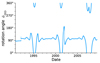 |
Fig. A.1. Rotation angle, ϕISD, of an inflow coming with a speed of vISD, ∞ = 26 km/s from the direction of the He inflow, (lHe, bHe) = (255.41° ,5.03° ), which has been taken from Swaczyna et al. (2018). Each blue circle corresponds to the value of the rotation angle at the start of each respective day. (After Hofstetter & Sieber 2021, Fig. 7.) |
Appendix B: Derivation of ISD properties
This appendix gives details on how to derive the ISD particle flux (Appx. B.1), the ISD flow direction (Appx. B.2), and the gas-to-dust mass ratio (Appx. B.3) from the measurements made by Ulysses (Grün et al. 2010).
B.1. Derivation of the ISD particle flux
The ISD particle flux is derived from the number of particles measured by the detector, N, per unit time, Δt, and per unit effective sensitive surface area averaged over Δt,  :
:
 (B.1)
(B.1)
For the Ulysses dust detector, the sensitive area, Asens, depends on the impact angle, α, which is the angle between the trajectory of the incoming dust particle and the boresight of the detector, also referred to as the angle of incidence,
 (B.2)
(B.2)
This is shown in Fig. B.1. Only for α = 0° the entire surface area of the detector is sensitive,  , and decreases for larger α until the opening angle of the detector, αmax = 70°, is reached, Asens(αmax) = 0 m2.
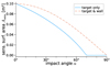 |
Fig. B.1. Sensitive surface area, Asens, of Ulysses’ dust detector over the impact angle, α, without (blue solid line) and with (red dashed line) considering wall impacts. Reproduced with permission after Altobelli et al. (2004, Fig. 6); copyright of the original figure by Elsevier. |
As Altobelli et al. (2004) noted, not only impacts on the detector target but also against the detector’s inner wall may lead to a successful measurement of the dust impact. If wall impacts are taken into account, the sensitive surface area is significantly higher and non-zero up to an opening angle of αmax = 90° (see Fig. B.1).
However, the detector is not at rest with respect to the impacting particles. Therefore, its effective sensitive surface area,
 (B.3)
(B.3)
also depends on the magnitude of the relative velocity between the spacecraft and the dust particle,
 (B.4)
(B.4)
where vU is the heliocentric velocity of Ulysses.
Thus, the effective sensitive surface area depends on the impact angle and on the relative velocity between the spacecraft and the dust particle, which in turn depends on the detector boresight and on Ulysses’ orbital position and velocity. In total, Aeff is determined depending on the rotation angle and on the date and time of impact.
This is illustrated by Fig. B.2 (see also Fig. A.1). The effective sensitive surface area is given with respect to a preferential direction, which here is the ISD inflow direction, and has the inflow speed of ISD as a parameter. Thus, this determination assumes that the dust inflow comes precisely from the ISD inflow direction with exactly vISD, ∞, meaning not only that the ISD inflow should be perfectly collimated, but also that it should not be influenced by any forces such as solar gravitation, solar radiation pressure, or the Lorentz force.
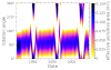 |
Fig. B.2. Effective sensitive surface area of the detector in relation to time and to the rotation angle, ϕrot. In this plot, ISD is assumed to be perfectly collimated, coming from (255.41° ,5.03° ) with 26 km/s. (After Janisch 2021, Fig. 2.10; see Landgraf 1998, Figs. 2.10 & 2.11.) |
Periods during which the dust instrument was switched off.
To calculate the average ISD flux during a finite time interval, the effective sensitive surface area must be averaged over that time interval and over the full rotation angle. The time-averaging must take into account gaps during which no ISD could be detected, some of which are caused by the exclusion criteria (cf. Sect. 3.1): the period before the Jovian flyby, the ecliptic crossings at Ulysses’ perihelion, and the Jovian dust streams.
Multiple instrument switch-offs also occurred (see Table B.1), during which no measurements could be taken. The first of these periods corresponds to the time interval between the launch of the spacecraft and the initialisation of the dust detector, and the last of these periods similarly corresponds to the time interval between the shutdown of the dust detector and the end of the mission. The in-between time periods were either caused by anomalies where all scientific instruments were shut down, or in later years by power-sharing between the various instruments. All these gaps have the effective function of instrumental dead times, meaning that they reduce Δt in Eq. (B.1). This is especially relevant for the measurements taken before 1994 and since 2002, when many causes for gaps occurred.
The averaging of  in Eq. (B.1) complicates the calculation of the flux: analytically,
  would be calculated with the integral over the time interval; numerically, it must be approximated by summation over finite steps of the time and rotation angle, Δt and Δϕrot, respectively. In practice, it has proven expedient to use Δt = 5 d and Δϕrot = 6°. Compared to calculations with Δt = 1 d and Δϕrot = 1° this introduces a maximum error of 0.2% while decreasing computational costs by one and a half magnitudes. Because the uncertainty of the flux (Appx. B.1.1) is generally much higher, this uncertainty is not taken into account. This determination of the ISD particle flux has been applied to the differently selected ISD subsets in Sect. 5.1.
B.1.1. Confidence interval of the ISD particle flux
The lower and upper limits, Fl, u, of the confidence interval of the ISD particle flux have been calculated in analogy to Eq. (B.1) by
 (B.5)
(B.5)
where λl, u are the lower and upper value of the expected number of ISD particle impacts during the respective time span, respectively. These values were determined under the assumption that ISD particle impacts are Poisson-distributed.
The Poisson distribution, Φ(λ, k), and its cumulative distribution function, CDF(Φ), are given by
 (B.6)
(B.6)
where k is the number of events (i.e. ISD particle impacts), and λ is a parameter that is identical to the variance of the distribution.
The cumulative distribution function is related to a given confidence level of  by (Gehrels 1986):
 (B.7)
(B.7)
In practice, λl, u are the λ that minimise the terms
 (B.8)
(B.8)
respectively. We note that the equation for the lower limit of Eq. (B.7) does not hold for N = 0; λl(N = 0) = 0 is used instead.
B.2. Derivation of the ISD flow direction
The precise direction from which an impacting particle came is not known. However, the particle must have come from the spherical sector spanned by the detector’s opening angle centred around the detector boresight at the time of impact, which is given by the rotation angle. The detector’s opening angle is 70° if wall impacts are not considered; when taking wall impacts into account, the detector’s field of view amounts to a full hemisphere (cf. Appx. B.1; Altobelli et al. 2004). By averaging over multiple ISD impacts, a more precise estimate of the rotation angle from which the ISD particles came can be made (Grün et al. 2001, Ch. II.D).
ISD particles are assumed to come from the ISD inflow direction. A good measure to evaluate this assumption is the average deviation of the detector’s rotation angle from the rotation angle corresponding to the ISD inflow direction, ϕISD (see Fig. A.1),
 (B.9)
(B.9)
where the circular mean has been used for averaging.
The uncertainty of this measure is given by
 (B.10)
where ϕrot(1σ) is the angle at which the effective sensitive area reaches the value of 1σ ≈ 68.27% of its maximum, and N is the number of impacts over which was averaged. The 1σ-angle is ϕrot(1σ) = 46.7° if wall impacts are taken into account, and 31.1° if they are not. This uncertainty is similar but not identical to the tabulated values provided by Grün et al. (2001, Table 3), as noted by Janisch (2021, Table 3.1). This has been applied to the differently selected ISD subsets in Sect. 5.2.
B.3. Calculation of the gas-to-dust mass ratio
In order to calculate the gas-to-dust mass ratio in the LISM, Rg/d = ρgas/ρISD, the gas mass density in the VLISM, ρgas, and the dust mass density measured by Ulysses, ρISD, must be known. Krüger et al. (2015) calculated the gas mass density from the hydrogen number density, nH, and the helium number density, nHe,
 (B.11)
where mH, He are the atomic masses of hydrogen and helium, respectively. They adopted a hydrogen number density of nH = 0.247 cm−3 (Slavin & Frisch 2008) and a helium number density of nHe = 0.015 cm−3 (Möbius et al. 2004), resulting in a gas mass density of ρgas ≈ 5.14 × 10⁻²² kg/m3. Their dust mass density of ρISD = (2.1 ± 0.6)×10−24 kg/m3 resulted in a gas-to-dust mass ratio of  (Krüger et al. 2015).28
Depending on which mass determination method is used (see Sect. 4), different values of Rg/d can be calculated. Following the approach of Landgraf (1998) and Krüger et al. (2015), the corresponding ISD subset is divided into sorted and ascending bins of the particle mass that count N = 30 particles each. The differential mass density distribution,
![Mathematical equation: $$ \begin{aligned} \mathcal{D} (m) :=&\ \frac{\mathrm{d} m}{V\,\mathrm{dlog} _{10}(m\,[\mathrm{kg}])} \end{aligned} $$](/articles/aa/full_html/2025/06/aa53532-24/aa53532-24-eq118.gif) (B.12)
(B.12)
![Mathematical equation: $$ \begin{aligned} \approx&\ \frac{\sum \limits _{i\in \mathrm{bin} }m_i}{V_{\mathrm{det} }\,\Delta (\log _{10}(m\,[\mathrm{kg}]))_{\mathrm{bin} }} =: \mathcal{D} _{\mathrm{bin} } \ , \end{aligned} $$](/articles/aa/full_html/2025/06/aa53532-24/aa53532-24-eq119.gif) (B.13)
(B.13)
is approximated by dividing the sum of all masses, mi, in the respective bin by the swept volume of the detector, Vdet, and the logarithmic width of the respective mass bin. The swept volume of the detector is calculated by integrating over the effective surface area of the detector during a given time interval, Eq. (B.3), multiplied with the distance the spacecraft has travelled in that time interval. From 29 October 1990 to 1 December 2007, taking into account the measurement gaps, this results in a swept volume of Vdet ≈ 3.15 × 10¹¹ m3. For the measurement-derived and iteratively calculated masses of the Krüger subset the resulting differential mass density distribution is shown in Fig. B.3.
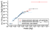 |
Fig. B.3. Differential mass density distribution for the measurement-derived masses, including (red) or excluding (black) the particles with vmsr < 3 km/s that most likely feature severely overestimated masses, and for the iteratively calculated masses (blue), of the Krüger subset in mass bins of N = 30 particles each. The horizontal error bars indicate the width of the mass bins, and the vertical error bars stem from the uncertainty of the mass determination, scaled by |

The uncertainty of the differential mass distribution, graphed as the vertical error bars of Fig. B.3, correspond to the uncertainty of the mass determination. Because the individual masses are known with an error factor of ∼10, that is, because their uncertainty is Δlog10(m [kg]) ≈ 1, the uncertainty of the sum of N masses,  , is
, is ![Mathematical equation: $ {\Delta}\log_{10}(M\,[\mathrm{kg}]) = 1/\sqrt{N} $](/articles/aa/full_html/2025/06/aa53532-24/aa53532-24-eq122.gif) .
.
Integrating over the differential mass density distribution, which corresponds to summing the value of each mass bin multiplied with the logarithmic width of that bin, gives the mass density of ISD:
![Mathematical equation: $$ \begin{aligned} \rho _{\mathrm{ISD} }&= \int \mathcal{D} (m)\,\mathrm{dlog} _{10}(m\,[\mathrm{kg}]) \end{aligned} $$](/articles/aa/full_html/2025/06/aa53532-24/aa53532-24-eq123.gif) (B.14)
(B.14)
![Mathematical equation: $$ \begin{aligned}&\approx \sum \limits _{\mathrm{bin} } \mathcal{D} _{\mathrm{bin} }\, \Delta (\log _{10} (m\,[\mathrm{kg}]))_{\mathrm{bin} } \end{aligned} $$](/articles/aa/full_html/2025/06/aa53532-24/aa53532-24-eq124.gif) (B.15)
(B.15)
This has been applied to the measurement-derived and the iteratively calculated masses in Sect. 6.4.
Appendix C: Reconstruction of the heliocentric ISD particle speed
In general, the heliocentric speed, vhel, of a dust particle encountered by Ulysses is not known; only the particle’s impact speed, vmsr, can be determined from the detector signal (cf. Sect. 4.1). If the heliocentric speed of the spacecraft, vU, as well as the angle between the two velocity vectors, χ, are known, the heliocentric speed of the dust particle can be reconstructed:
 (C.1)
(C.1)
where χ is the angle between the detector boresight and the spacecraft’s direction of motion (cf. Appx. A). An angle of χ = 0° corresponds to a particle impacting the spacecraft head-on with respect to the spacecraft’s direction of motion, meaning that the dust particle moves anti-parallel to the spacecraft. For χ = 180° the dust particle would impact the spacecraft’s aft. The precision of the determined impact speed, vmsr, is given by a multiplicative error factor, errv, and the precision of χ is given by the opening angle of the detector, αmax.
C.1. Relevance of the detector’s opening angle
The role that these uncertainties play in the reconstruction of the particle’s heliocentric speed depends strongly on how the spacecraft speed, vU, compares to the dust particle’s heliocentric speed, vhel, and on the angle between the detector boresight and the spacecraft’s direction of motion, χ.
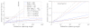 |
Fig. C.1. Worst-case error factor of the reconstructed heliocentric speed, |

ISD particles, which follow hyperbolic heliocentric orbits, are usually faster than the spacecraft, which follows an elliptical orbit,29vhel > vU. If the spacecraft speed is negligible compared to the speed of the dust particle, vU ≪ vhel, the detector’s opening angle is of little relevance, and the reconstructed heliocentric speed is almost identical to the determined impact speed, vrec, hel ≈ vmsr, irrespective of χ. The reconstruction of the heliocentric speed will be as accurate as the impact speed determination is precise, and the opening angle of the detector only limits the precision by which the direction of origin is known.
However, if the speeds of the spacecraft and of the dust particle are similar, the reconstructed heliocentric speed of Eq. (C.1) strongly depends on the angle χ between the spacecraft’s and the dust particle’s velocity vectors. The finite opening angle of the detector introduces another uncertainty to the reconstructed heliocentric speed, Δvrec, hel. How large this uncertainty is depends not only on the detector’s opening angle, αmax, but also on the heliocentric speed of the spacecraft, vU, and on χ itself.
The uncertainty of the determined impact speed, vmsr, is given by a multiplicative error factor, errv (cf. Sect. 3). The uncertainty of the reconstructed heliocentric speed that is introduced by the finite opening angle of the detector can be represented by an error factor as well, which we name errα. Using Eq. (C.1) with a given impact speed, vmsr, and a given spacecraft speed, vU, leads to the definition of this error factor as
![Mathematical equation: $$ \begin{aligned} \mathrm{err} _{\alpha }:=\frac{v_{\mathrm{rec,hel} }(\chi +\alpha )}{v_{\mathrm{rec,hel} }(\chi )}\ ,\ \left\{ \begin{array}{l}\chi \in [{0}^\circ , {360}^\circ ] \\ \alpha \in [{0}^\circ ,\alpha _{\max }]\end{array}\right. \ , \end{aligned} $$](/articles/aa/full_html/2025/06/aa53532-24/aa53532-24-eq127.gif) (C.2)
(C.2)
which represents the factor by which the reconstructed heliocentric speed changes if the angle χ has been overvalued by α ∈ [0° ,αmax]. To reiterate, χ ∈ [0° ,360° ] is the angle between the spacecraft’s direction of motion and the direction from which the particle comes, and α ∈ [0° ,αmax] is the angle by which the detector’s boresight deviates from the particle’s incoming direction.
In most cases, for example on Ulysses, neither χ nor α are constrained more than is stated in Eq. (C.2), and the error factor varies for a given spacecraft speed, particle speed, and detector opening angle. Therefore, it is convenient to give the worst-case error factor,  ; in other words, to maximise errα over all χ and α. The angles that maximise errα correspond to the spacecraft’s and the particle’s least favourable directions of motion for the purpose of accurately reconstructing the dust particle’s heliocentric speed from the determined impact speed.30
C.2. Application to the orbits of Earth, Jupiter, and Ulysses
Examples of how the worst-case error factor of the reconstructed heliocentric speed,  , changes with the opening angle of the detector are plotted in Fig. C.1 for circular orbits of Earth and Jupiter for the cases where the spacecraft moves antiparallel to the ISD direction (particles impacting the bow of the spacecraft at high impact speed) and parallel to the ISD direction (particles impacting the aft of the spacecraft at low impact speed). The cases of Ulysses at its aphelion and perihelion, perpendicular to the ISD particles’ motion, are plotted as well.
In order to distinguish ISD from IDPs, the error factor must lie below an upper limit: assuming that ISD moves with vhel as per Eq. (4) and that an extremely eccentric OCC particle moves with (almost) vesc as per Eq. (5), the error factor must lie below vhel/vesc|r = 1 au ≲ 1.18 at Earth and vhel/vesc|r = 5.2 au ≲ 1.73 at Jupiter; the reconstructed heliocentric speed must be known within these accuracies. To distinguish an ISD particle from an IDP on a circular orbit, these accuracy limits would be 1.66 at Earth and 2.44 at Jupiter.
As Fig. C.1 shows, the worst-case error factor,  , increases almost linearly with the opening angle until approximately
  . The error factor for Ulysses with an opening angle of
  is 1.36 at its aphelion and 3.83 at its perihelion. For an opening angle of
  , the worst-case error factors are 1.46 at the aphelion and 4.62 at the perihelion, assuming that the spacecraft’s motion is perpendicular to the ISD particle’s trajectory.
For spacecraft on orbits in or close to the ecliptic plane, the worst-case error factor changes during the spacecraft orbit: when the spacecraft moves roughly antiparallel to the ISD inflow, the relative speed between the detector and the dust particle is highest; that is, ISD particles impact at high speeds. Thus, as per Eq. (C.1), a wider opening angle is sufficient to distinguish ISD from IDPs. Conversely, during an orbital section where the spacecraft moves roughly parallel to the ISD inflow, a smaller opening angle is required to unambiguously distinguish ISD from IDPs.
For spacecraft on a roughly circular orbit similar to Earth, ISD particles can be distinguished from extremely eccentric cometary dust particles along the entire orbit of the spacecraft if the direction of origin of a given particle is known with a precision better than  . If this precision is
  , ISD particles and extremely eccentric cometary particles cannot be distinguished even when the spacecraft moves antiparallel to the ISD inflow direction. For spacecraft on Jupiter-like orbits, these critical angles increase to
  and
and  , respectively. This assumes that the impact speed can be determined with perfect accuracy, or, in other words, that the error factor of the impact speed determination is errv = 1.0, which is not the case.
C.3. Relevance of the uncertainty of the measurement-derived impact speed
The two error factors,  and errv, which are introduced by the finite opening angle and by the error factor of the impact speed determination, respectively, are at most multiplicative but not necessarily so. The faster the spacecraft speed is compared to the particle’s impact speed, the less influential the determined impact speed is in Eq. (C.1): for vU ≫ mmsr the impact speed barely affects the reconstructed heliocentric speed, and the error factor of the determined impact speed has no significant bearing on the uncertainty of the reconstructed heliocentric speed. Thus, the total error factor, errtot, is at least identical to the error factor introduced by the opening angle,
  , and at most the product of
  and the error factor introduced by the impact speed determination, errv;
 (C.3)
(C.3)
Using the equality in Eq. (C.3) serves as a conservative estimate of the total error factors and is used in the following.
When using the product of both error factors, the precision of the reconstructed heliocentric speed is 1.36 ⋅ 1.9 ≈ 2.58 at Ulysses’ aphelion for an opening angle of 70°, which is insufficient to distinguish ISD particles from particles on parabolic or even circular orbits. However, depending on the detector boresight, the total error factor may be considerably smaller than this conservative estimate. Larger-number statistics are also an aid in narrowing down the direction of origin of many particles with similar trajectories (e.g. Gehrels 1986).
Nevertheless, the closer to the Sun, the more the total error factor increases, and the more the required precision tightens. At Ulysses’ perihelion, for example, the worst-case error factor is  , and thus the heliocentric particle speed can only be reconstructed within an accuracy of
  for errv = 1.9, which does not allow for any differentiation between ISD from dust on parabolic or even circular orbits.
This illustrates once again that a more precise determination of both the impact speed and the direction of origin would be an invaluable improvement, especially for distinguishing between different origins of dust (cf. Sect. 6.2.1).
Applying the above considerations to the DESTINY+ Dust Analyser (DDA), assuming an angular accuracy of 10° and a speed error factor of 1.1 on a roughly Earth-like orbit (Simolka et al. 2024), results in a total worst-case error factor of 1.08 when moving against the ISD inflow direction and 1.22 when moving with the ISD inflow direction. This should allow DDA to comfortably distinguish ISD from particles on circular orbits throughout the entire spacecraft orbit. Particles on highly eccentric (i.e. near-parabolic) orbits should be distinguishable from ISD during the half-orbit when DESTINY+ moves partially against the ISD inflow direction. During the other half-orbit where the spacecraft moves partially parallel to the ISD inflow, a clear identification of ISD by its reconstructed heliocentric speed may be more ambiguous.
We note that this analysis assumes that gravitation is dominant over solar radiation pressure and the Lorentz force (i.e. β ≈ 0 and Q/m ≈ 0). This is a reasonable assumption for silicate grains of all porosities but not for carbonaceous grains (see Fig. 1; see also Kimura 2017). The inclusion of solar radiation pressure will decrease the local escape speed and thus allow for larger error factors before ISD particles can no longer be identified. However, at least in the context of Ulysses’ most massive particles, this yielded no significant changes even for highly porous, carbonaceous grains (Sect. 6.2.2).
Appendix D: Details of the methodology to investigate the heliosheath filtering function
This appendix details how the measured size distribution was determined from Ulysses’ measurements (Appx. D.1) and how the numerical simulations were performed (Appx. D.2), and presents the time-dependent modulation of the ISD flux by forces in the inner heliosphere (Appx. D.3) and the time-dependent detector transfer function (Appx. D.4).
D.1. Details of the determination of the measured size distribution
A differential size distribution, dn/da, describes the number density of particles, n, in an infinitesimal size bin, a ∈ [a; a + da]. The number of particles within a finite size interval, (Δa)i = [ai, ai + 1] that, during the time interval (Δt)i = [ti, ti + 1], move through an area, A, perpendicular to their direction of motion with a speed of vd is given by
 (D.1)
(D.1)
or, assuming that measurements can only be taken in finite bins of size and time, by
 (D.2)
(D.2)
where Δn/Δa indicates the average of dn/da over the respective size bin and time bin. Correspondingly, the differential size distribution measured by a spacecraft, (Δn/Δa)obs, in size bin (Δa)i is
 (D.3)
(D.3)
where N(Δa)i, (Δt)i is the number of particles measured within size bin (Δa)i and time bin (Δt)i, and Amax is the surface area of the detector.
In order to apply the filtering and modulation functions to this differential size distribution, the size bins of Eq. (D.3) must correspond to the sizes available for the numerical simulations. The simulated parameter sets, (β, Q/m), listed in Table D.1, are equidistant in log(a), forming the centres of equidistant logarithmic size bins of the width δlog(a [μm]) ≈ 0.1278.
D.2. Details of the numerical simulations used to infer the ISD filtering in the heliosheath
The modulation of the differential size distribution due to the forces in the inner heliosphere, fF (cf. Sect. 7.3), is investigated with the numerical simulation code IMEX (Sterken et al. 2015; Strub et al. 2019), which has been verified by comparison with measurements taken by various spacecraft (Krüger et al. 2019).
In this instance, the code launches ISD particles from the heliocentric direction of (l, b) = (259° ,8° ) with a uniform speed of 26 km/s, with their initial positions randomised on a plane perpendicular to the velocity vector with a distance of 50 au to the Sun (Strub et al. 2019). The particles’ position and velocity are numerically advanced in time under the effect of solar gravitation, solar radiation pressure, and the Lorentz force.
For the Lorentz force, only the interplanetary magnetic field is taken into account. The magnetic field is simulated by a modified Parker spiral (Parker 1958). Its polarity depends on the phase of the solar magnetic cycle and the position of the dust particle with respect to the heliospheric current sheet, averaged over one solar rotation (Sterken et al. 2012a; Strub et al. 2019).
The simulation domain is separated into a heliocentric, equidistant, cubic grid with a spatial resolution of 0.25 au per grid cell edge, spanning a total volume of (20 au)3. The temporal resolution is 12.2 d.
For each item in a set of dust species, parametrised by their β-ratio and charge-to-mass ratio, (β, Q/m), 2 × 10⁹ trajectories were calculated. The time-resolved number densities, average particle velocities, and the velocity dispersion for each grid cell are saved.
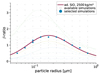 |
Fig. D.1. β-curves of Fig. 1 against the particle radius, available simulation sets of (β, Q/m) (grey dots), and the selected simulation sets (blue circles) that are closest to the β-curve of the adapted astronomical silicates with ρd = 2500 kg/m3 (maroon line). (See Hunziker et al., in prep.; after Sterken et al. 2013, Fig. 3.) |
Simulations were computed only for certain values of (β, Q/m), so simulations with the values closest to the assumed β-curve have to be selected to approximate the full size range of a particle distribution. Fig. D.1 shows the β-curves of Fig. 1, given in relation to the particle radius, a, and both the available and the selected tuples of (β, Q/m). For this, the charge-to-mass-ratio, Q/m, was converted to the particle radius, a, with the relation
 (D.4)
(D.4)
where ε0 is the electric constant and U = +5 V is the assumed surface potential of the dust particles. We note that no dynamic charging of the dust particles is included at this time, and Q/m is therefore constant. This is valid within ca. 50 au due to a decrease in the plasma density and the UV flux with the squared distance to the Sun. Eq. (D.4) follows directly from the equations for the surface charge of a spherical particle, Q = 4πε0aU, and for the mass of a compact, spherical particle, m = 4π/3 ρda3.
Parameters of the numerical simulations.
The selected sets of (β, Q/m) are listed in Table D.1. For convenience, conversions to the particle mass and radius have been provided in that table as well. We note that two sets of (β, Q/m) were simulated for a ≈ 9.29 × 10⁻² μm because the assumed β-curve for that size lies in-between two available parameter sets. For this particle size, the results will be averaged over both sets.
The modulation of the differential size distribution due to the forces in the inner heliosphere, fF, is the density enhancement factor, n/nISM, which is directly given as an output of the simulation, depending on both heliocentric coordinates, r, and time, t. Along the orbit of a spacecraft, for example Ulysses, the appropriate coordinates change with time, r(t), and thus fF(a) depends only on time, Eq. (11).
D.3. Time-dependent modulation of the ISD flux by forces in the inner heliosphere
Fig. D.2 shows the change of the modulation due to inner heliosphere forces, fF, over time for four selected particle sizes: a ≈ 2.30 μm, which are the largest simulated particles; a ≈ 4.07 × 10⁻¹ μm, which are the particles with β = 1; a ≈ 1.67 × 10⁻¹ μm, which are the particles with the highest β-ratio, β = 1.5; and a ≈ 5.15 × 10⁻² μm, which are the smallest simulated particles.
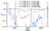 |
Fig. D.2. Time-dependent modulation by the inner heliosphere forces, fF, of the ISD flux that reaches Ulysses compared to the ISD flux at the termination shock, for four sets of parameters, (β, Q/m), corresponding to particle sizes of a ≈ 2.30 μm (dashed grey line), a ≈ 4.07 × 10⁻¹ μm (dash-dotted navy line), a ≈ 1.67 × 10⁻¹ μm (dotted red line), and a ≈ 5.15 × 10⁻² μm (solid blue line): daily values in a moving average of 31 d. The shaded areas correspond to the perihelion crossings. |
For the largest particles (β = 0.2, Q/m = 0.01 C/kg), the simulations result in virtually no modulation; the density enhancement factor is n/nISM ≈ 1, independent of the phase of the solar cycle.
The particles with β = 1, which do not experience solar gravitation or solar radiation pressure but are affected by the Lorentz force, show a dip to, at its minimum, 40% of the ISM density from 1997 to 2002, following the solar minimum of the defocusing phase of mid-1996 (Sterken et al. 2015; cf. Table 4), and an increase by a factor of two to three during the perihelion crossing of 2007.
The smaller particles are more strongly modulated. As expected, for β > 1 no particles reach into the β-cones (fF = 0), as evidenced by the gaps surrounding the perihelion crossings. During the times of defocusing, beginning one to two years after the solar minimum of the defocusing phase in mid-1996, particles are strongly depleted (fF < 0.1) but steadily increase until the solar minimum of the focusing phase in late 2008, which coincides with the final perihelion crossing of 2007 before the dust detector was switched off at the end of November 2007. Surrounding the perihelion crossing of 2001, slightly higher densities compared to the adjacent times can be observed because particles gather at the outer edges of the β-cones (Sterken et al. 2013). Preceding the first perihelion crossing, the particles are strongly enhanced (fF ≈ 10). This can be attributed to the trailing flank of the solar minimum of the focusing phase of 1986.
The smallest particles (β = 0.50, Q/m = 20 C/kg) show a similar variation. As the solar cycle changes from its maximum in 1989 to the minimum of the defocusing phase in 1996, these particles are more and more depleted; and as the solar cycle changes to its minimum of the focusing phase in late 2008, this depletion becomes weaker. Only during the perihelion crossing in 2007, adjacent to the solar minimum of the focusing phase in late 2008, the particle density is enhanced up to a factor of fF = 3.
The variability in time of the modulation by the inner heliosphere forces, fF, illustrates that care must be taken when averaging over time, as will be necessary for most applications. A more detailed analysis of the modulation of particles of different sizes due to the forces in the inner heliosphere applied to Ulysses is given by Landgraf et al. (2000), Sterken et al. (2015).
D.4. Time-dependent detector transfer function
As stated in Sect. 7.4, the time-dependent detector transfer function depends on the angle of incidence between the detector boresight and the particle motion, and on the relative speed between the dust particle and the spacecraft, Eq. (12). The numerical simulations were used to determine the velocity vector of the dust particle. However, only the average velocity of all dust particles within the respective model cell is available. This average can strongly differ from the individual particle velocities. This happens, for example, when averaging two opposing velocity vectors in the gravitational focusing region downstream of the Sun.
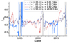 |
Fig. D.3. Time-dependent detector transfer function, fdet, of the ISD flux that can be measured compared to the ISD flux that reaches Ulysses, for the same four parameter sets as in Fig. D.2, corresponding to particle sizes of a ≈ 2.30 μm (dashed grey line), a ≈ 4.07 × 10⁻¹ μm (dash-dotted navy line), a ≈ 1.67 × 10⁻¹ μm (dotted red line), and a ≈ 5.15 × 10⁻² μm (solid blue line), using daily data points. |
The resulting transfer function has been plotted in Fig. D.3 for the same four parameter sets as in Fig. D.2. In analogy to Appx. B.1, Aeff was averaged over the rotation angle and over time. Because the ISD velocity vector has been taken from the numerical simulations, the transfer function cannot be derived if there is no simulation data available, for instance within the β-cone.
The detector transfer function typically lies between 0.2 ≤ fdet ≤ 0.5 but does reach significantly higher values for the smallest particles (β = 0.5, Q/m = 20 C/kg) surrounding the first perihelion crossing in early 1995. For the largest particles (β = 0.2, Q/m = 0.01 C/kg) and even more so for the particles with β = 1, the average velocity vector is similar to the ISD inflow vector. For smaller particles the Lorentz force deflects the particles from their initial orbits more strongly.
D.4. Determination of statistical uncertainties for Sect. 7
The determination of the heliosheath filtering function fh has multiple sources of uncertainty. Some of these uncertainties are graphed as error bars in Figs. 11 and 12. These error bars are calculated as follows:
Fig. 11a shows the measured differential size distribution, (Δn/Δa)obs, which is calculated with Eq. (D.3). There, N(Δa)i, (Δt)i = :N is the number of particles within size bin (Δa)i measured during time bin (Δt)i, which we assume to be Poisson-distributed for the sake of simplicity. Hence, its uncertainty is the Poissonian standard deviation, which is the square root of the respective number of particles,  . To calculate the uncertainty of (Δn/Δa)obs, we Gauss-propagate this standard deviation of N through Eq. (D.3), which is identical to replacing N with
  and results in
![Mathematical equation: $$ \begin{aligned} \Delta \left[\left(\frac{\Delta n}{\Delta a}\right)_{\mathrm{obs} }\right] \approx \frac{\sqrt{N_{(\Delta a)_i, (\Delta t)_i}}}{A_{\max }\cdot v_{\mathrm{d} }\cdot (\Delta t)_i\cdot (\Delta a)_i} \ . \end{aligned} $$](/articles/aa/full_html/2025/06/aa53532-24/aa53532-24-eq150.gif) (D.5)
(D.5)
These values have been plotted as vertical error bars in Fig. 11a.
Fig. 11d shows the inferred differential size distribution at the termination shock, (Δn/Δa)TS, which was calculated following Eq. (9):
 (D.6)
(D.6)
Its uncertainty has been Gauss-propagated from Eq. (D.6),
![Mathematical equation: $$ \begin{aligned} \Delta \left[\left(\frac{\Delta n}{\Delta a}\right)_{\mathrm{TS} }\right] = \frac{1}{\bar{f}_{F}(a) \cdot \bar{f}_{\mathrm{det} }(a)} \cdot \Delta \left[\left(\displaystyle \frac{\Delta n}{\Delta a}\right)_{\mathrm{obs} }\right] \ , \end{aligned} $$](/articles/aa/full_html/2025/06/aa53532-24/aa53532-24-eq152.gif) (D.7)
(D.7)
and plotted as vertical error bars in Fig. 11d.
Fig. 12 shows the size-dependent and time-averaged heliosheath filtering function,
 (D.8)
(D.8)
where (dn/da)ISM has been calculated with Eq. (10) for the geometric mean of the respective size bin. Its uncertainty follows directly from Eq. (D.8) by replacing (Δn/Δa)TS with its uncertainty:
![Mathematical equation: $$ \begin{aligned} \Delta \bar{f}_{\mathrm{hs} }(a)= \frac{\Delta \left[\left(\Delta n/\Delta a\right)_{\mathrm{TS} }\right]}{(\mathrm{d} n/\mathrm{d} a)_{\mathrm{ISM} }} \end{aligned} $$](/articles/aa/full_html/2025/06/aa53532-24/aa53532-24-eq154.gif) (D.9)
(D.9)
These values have been plotted as vertical error bars in Fig. 12. Additional uncertainties that have not been taken into account when calculating the error bars are discussed in Sect. 7.7.
Appendix E: Properties of Subset B
Table E.1 gives the properties of the particles of Subset B (Sect. 6.3) in analogy to Table 1. Table E.2 lists the reconstructed heliocentric speeds for the particles of Subset B in analogy to Table 2.
Properties of the particles of Subset B in analogy to Table 1.
Reconstructed heliocentric speed for each particle of Subset B (see Table E.1) in analogy to Table 2.
All Tables
Reconstructed heliocentric speed for each particle of Subset B (see Table E.1) in analogy to Table 2.
All Figures
|
Fig. 1. β-curves for amorphous carbon (‘C’, green lines, Kimura & Mann 1999), astronomical silicates (“SiO”, solid gold line, Gustafson 1994; and blue lines, Kimura & Mann 1999), and adapted astronomical silicates (“ad. SiO”) with an assumed dust density of ρd = 2500 kg/m3 (thick dashed maroon line; Sterken et al. 2012a). The β-curves of Kimura & Mann (1999) have porosities, p, ranging from 0% (compact particles) to 93% (fluffy particles), indicated by different line styles. (After Sterken et al. 2015, Fig. 2.) |
| In the text | |
|
Fig. 2. Three-dimensional depiction of the orbits of Ulysses (solid black line), Jupiter (dashed ochre line), and Earth (dash-dotted blue line) in heliocentric ecliptic coordinates. The +x-direction points towards the vernal equinox, and the +z-direction points to ecliptic north. The Sun is marked as a yellow star. The faint grey curves on the coordinate planes are projections of Ulysses’ orbit onto that plane (see Fig. 3). The dark grey lines close to the almost-horizontal and vertical axes are projections of the homogeneous ISD inflow coming from (l, b) = (255.41° ,5.03° ) onto the xy- and xz-planes. (See Krüger et al. 2015, Fig. 1.) |
| In the text | |
|
Fig. 3. Ulysses orbit projected onto the xz- (left) and yz-plane (right), colour-coded according to heliocentric speed. Jupiter’s and Earth’s orbits are indicated as dashed green and dotted blue lines, respectively. The dark grey arrows indicate projections of the ISD inflow direction and are identically scaled in both panels. (See Landgraf 1998, Fig. 2.5.) |
| In the text | |
|
Fig. 4. Uptime of the dust detector with respect to measuring ISD covering the full duration of the Ulysses mission. Shaded areas denote times when the dust detector was turned off (‘off’, top row, red), when data were excluded due to time spent in the ecliptic plane (‘ecl’, middle row, blue), and when data were excluded due to Jovian streams (‘Jov’, bottom row, green). |
| In the text | |
|
Fig. 5. Interstellar dust particle flux for the union (blue circles), Krüger (orange triangles), Strub (green squares), and intersect (violet diamonds) subsets. The data have been aggregated in bins of Δt = 4 months, starting on 1 January 1992, with consideration of the measurement gaps (i.e. the detector dead times), which are indicated by the areas shaded in grey. Horizontal error bars denote the width of the time bin; vertical error bars were calculated as per Appendix B.1.1. Letters at the figure’s top indicate the time of Ulysses’ closest approaches to Jupiter (J), the spacecraft’s perihelia (P), and its aphelia (A). Wall impacts were taken into account for the detector’s sensitivity profile (cf. Fig. B.1), and for the dust kinematics, an inflow direction of (l, b) = (255.41° ,5.03° ) with a speed of vISD, ∞ = 26 km/s was assumed (Swaczyna et al. 2018). (After Janisch 2021, Fig. 5.7.) |
| In the text | |
|
Fig. 6. Mean deviation of each events’ rotation angle, ϕrot, from the rotation angle corresponding to the ISD inflow vector, ϕISD, for the union (blue circles), the Krüger (orange triangles), the Strub (green squares), and the intersect (violet diamonds) subsets, averaged over Δt = 4 months beginning on 1 January 1992. Horizontal error bars denote the width of the time bin, and vertical error bars were calculated with Eq. (B.10), taking into account wall impacts (cf. Fig. B.1). Grey-shaded areas and letters at the top edge are as in Fig. 5. (After Janisch 2021, Fig. 5.17.) |
| In the text | |
|
Fig. 7. Impact speed and particle mass determined by the measurement-derived method used in the dataset (green circles and black stars), by the approximate method that assumed β ≡ 1 (blue triangles), and by the iterative method (red crosses) using the union subset. The second and third methods assumed an inflow speed of vd = 26 km/s from the direction (lHe, bHe), and the iterative method further utilised the β-curve of adapted astronomical silicates (see Fig. 1). The measurement-derived values for impacts with vmsr < 3 km/s (black stars) most likely feature severely underestimated impact speeds and severely overestimated particle masses. We note that the horizontal axis quantifies the impact speed in the spacecraft frame and not the heliocentric speed. |
| In the text | |
|
Fig. 8. Mass distribution of the Krüger (thick solid blue line), Strub (dashed red line), union (dotted indigo line), and intersect (dash-dotted maroon line) subsets for the masses derived from measurements (panel a; cf. Sect. 4.1), approximated with β ≡ 1 (panel b; cf. Sect. 4.2), and calculated iteratively (panel c; cf. Sect. 4.3) with an assumed density of ρd = 2500 kg/m3. Measurement-derived masses corresponding to vmsr < 3 km/s were not taken into account (cf. Sect. 4.1). (See Krüger et al. 2015, Fig. 5, and Janisch 2021, Fig. 5.32.) |
| In the text | |
|
Fig. 9. Iteratively calculated mass, miter, versus measurement-derived mass, mmsr, for all particles of the union subset (small circles). The marker colours denote the measurement-derived impact speeds, vmsr. Particles with impact speeds below vmsr ≤ 3 km/s are highlighted as crosses. For these particles, the measurement-derived impact speeds are most likely severely underestimated, and thus the measurement-derived particle masses are severely overestimated (cf. Sect. 4.1). Different clusters of most massive particles, A1, 2, 3, aggregated to Subset A, are highlighted as squares; these particles are numbered 1–10. Another subset of massive particles, Subset B (Sect. 6.3), is marked by triangles. The dotted diagonal line denotes mmsr = miter. |
| In the text | |
|
Fig. 10. Ulysses’ orbital position and the detector’s boresight and cone of view at the times of the most massive particle impacts in the ecliptic xz- (left) and yz-plane (right). The detector boresight and its cone of view were Galilean-transformed from the spacecraft frame to the heliocentric frame, which distorts the cones of view. The Galilean transformation assumes that the dust particles’ relative velocity corresponds to the inverse boresight direction and either the measurement-derived impact speeds, vmsr (top), or the iteratively calculated impact speeds, viter (bottom). The ISD inflow is marked by grey arrows (see Fig. 3). The orbital positions at which the particles of Subset A impacted are indicated by blue squares, red triangles, and green circles for A1, 2, 3, respectively. The black lines point in the detector boresight, scaled identically in both panels. The coloured areas give the outer edge of the cone of view with an opening angle of ±70°, corresponding to the detector’s sensitivity without considering wall impacts. We note that the measurement-derived impact speeds are most likely spurious for the particles of A1, 2, and that the iteratively calculated relative speeds assume an ISD origin. Particles are numbered as in Fig. 9. The deviation of the boresight from the ISD inflow direction is tabulated in Table 2. |
| In the text | |
|
Fig. 11. Measurement-derived differential size distribution, (Δn/Δa)obs (panel a); time-averaged modulation factor through forces in the Solar System, |
| In the text | |
|
Fig. 12. Heliosheath filtering function, Eq. (9), in relation to the particle size, for the same time periods as Fig. 11, for the union subset with measurement-derived masses (panel a), for the Strub subset with measurement-derived masses (panel b), and for the union subset with iteratively calculated masses (panel c). The vertical error bars correspond to the (assumed) Poissonian standard deviation of the number of particles within the respective size and time bin (cf. Appendix D.5), (see Hunziker et al., in prep.). |
| In the text | |
|
Fig. A.1. Rotation angle, ϕISD, of an inflow coming with a speed of vISD, ∞ = 26 km/s from the direction of the He inflow, (lHe, bHe) = (255.41° ,5.03° ), which has been taken from Swaczyna et al. (2018). Each blue circle corresponds to the value of the rotation angle at the start of each respective day. (After Hofstetter & Sieber 2021, Fig. 7.) |
| In the text | |
|
Fig. B.1. Sensitive surface area, Asens, of Ulysses’ dust detector over the impact angle, α, without (blue solid line) and with (red dashed line) considering wall impacts. Reproduced with permission after Altobelli et al. (2004, Fig. 6); copyright of the original figure by Elsevier. |
| In the text | |
|
Fig. B.2. Effective sensitive surface area of the detector in relation to time and to the rotation angle, ϕrot. In this plot, ISD is assumed to be perfectly collimated, coming from (255.41° ,5.03° ) with 26 km/s. (After Janisch 2021, Fig. 2.10; see Landgraf 1998, Figs. 2.10 & 2.11.) |
| In the text | |
|
Fig. B.3. Differential mass density distribution for the measurement-derived masses, including (red) or excluding (black) the particles with vmsr < 3 km/s that most likely feature severely overestimated masses, and for the iteratively calculated masses (blue), of the Krüger subset in mass bins of N = 30 particles each. The horizontal error bars indicate the width of the mass bins, and the vertical error bars stem from the uncertainty of the mass determination, scaled by |
| In the text | |
|
Fig. C.1. Worst-case error factor of the reconstructed heliocentric speed, |
| In the text | |
|
Fig. D.1. β-curves of Fig. 1 against the particle radius, available simulation sets of (β, Q/m) (grey dots), and the selected simulation sets (blue circles) that are closest to the β-curve of the adapted astronomical silicates with ρd = 2500 kg/m3 (maroon line). (See Hunziker et al., in prep.; after Sterken et al. 2013, Fig. 3.) |
| In the text | |
|
Fig. D.2. Time-dependent modulation by the inner heliosphere forces, fF, of the ISD flux that reaches Ulysses compared to the ISD flux at the termination shock, for four sets of parameters, (β, Q/m), corresponding to particle sizes of a ≈ 2.30 μm (dashed grey line), a ≈ 4.07 × 10⁻¹ μm (dash-dotted navy line), a ≈ 1.67 × 10⁻¹ μm (dotted red line), and a ≈ 5.15 × 10⁻² μm (solid blue line): daily values in a moving average of 31 d. The shaded areas correspond to the perihelion crossings. |
| In the text | |
|
Fig. D.3. Time-dependent detector transfer function, fdet, of the ISD flux that can be measured compared to the ISD flux that reaches Ulysses, for the same four parameter sets as in Fig. D.2, corresponding to particle sizes of a ≈ 2.30 μm (dashed grey line), a ≈ 4.07 × 10⁻¹ μm (dash-dotted navy line), a ≈ 1.67 × 10⁻¹ μm (dotted red line), and a ≈ 5.15 × 10⁻² μm (solid blue line), using daily data points. |
| In the text | |
Current usage metrics show cumulative count of Article Views (full-text article views including HTML views, PDF and ePub downloads, according to the available data) and Abstracts Views on Vision4Press platform.
Data correspond to usage on the plateform after 2015. The current usage metrics is available 48-96 hours after online publication and is updated daily on week days.
Initial download of the metrics may take a while.