| Issue |
A&A
Volume 687, July 2024
|
|
|---|---|---|
| Article Number | L4 | |
| Number of page(s) | 9 | |
| Section | Letters to the Editor | |
| DOI | https://doi.org/10.1051/0004-6361/202450257 | |
| Published online | 25 June 2024 | |
Letter to the Editor
The unexpected role of heliospheric boundaries in facilitating interstellar dust penetration at 1–5 AU
1
Space Research Institute of Russian Academy of Sciences, Profsoyuznaya 84/32, Moscow 117997, Russia
e-mail: This email address is being protected from spambots. You need JavaScript enabled to view it.
2
Lomonosov Moscow State University, Moscow Center for Fundamental and Applied Mathematics, GSP-1, Leninskie Gory, Moscow 119991, Russia
3
Ishlinsky Institute for Problems in Mechanics of Russian Academy of Sciences, Vernadskogo 101-1, Moscow 119526, Russia
4
Faculty of Physics, HSE University, 20 Myasnitskaya Ulitsa, Moscow 101000, Russia
Received:
5
April
2024
Accepted:
11
June
2024
Abstract
Aims. Interstellar dust (ISD) particles penetrate the heliosphere because of the relative motion of the local interstellar cloud and the Sun. The penetrated particles pass through the heliospheric interface, that is, the region in which solar wind and interstellar plasma interact. As a result, the ISD flow is modified after the passage through this region under the influence of electromagnetic force. The main goal of this work is to show how the heliospheric interface affects the distribution of ISD particles near the Sun.
Methods. We have developed a Monte Carlo model of the ISD distribution in the heliosphere. It first takes the effects of the heliospheric interface and the rotating heliospheric current sheet into account. The effects of the heliospheric interface were probed using a global heliospheric model.
Results. The computation results show that the heliospheric interface strongly influences the distribution of relatively small (radius a = 150 − 250 nm) astronomical silicates. The unexpected finding is that the heliospheric interface facilitates the penetration of a = 150 nm particles at small heliocentric distances and, particularly, to the Ulysses orbit (1 − 5 AU). We demonstrate that the deflection of ISD particles in the outer heliosheath is the principal mechanism that causes the effects of the heliospheric interface on the distribution near the Sun. The computations with different heliospheric models show that the distribution near the Sun is sensitive to the plasma parameters in the pristine local interstellar medium. Thus, we demonstrated that being measured near the Sun, the ISD may serve as a new independent diagnostics of the local interstellar medium and the heliospheric boundaries.
Key words: Sun: heliosphere / dust, extinction
© The Authors 2024
 Open Access article, published by EDP Sciences, under the terms of the Creative Commons Attribution License (https://creativecommons.org/licenses/by/4.0), which permits unrestricted use, distribution, and reproduction in any medium, provided the original work is properly cited.
This article is published in open access under the Subscribe to Open model. This email address is being protected from spambots. You need JavaScript enabled to view it. to support open access publication.
1. Introduction
The Sun moves through the surrounding interstellar medium with a bulk velocity of ∼26.4 km s−1 (Witte 2004). In the solar reference frame, the supersonic solar wind emitted from the Sun interacts with the supersonic flow of partially ionized local interstellar medium (LISM) plasma (Baranov & Malama 1993), and as a result, a complex structure forms that consists of two shock waves (the heliospheric termination shock, TS, and interstellar bow shock, BS) and tangential discontinuity (heliopause, HP). The interaction region between the two shock waves is called the heliospheric interface. However, the existence of a bow shock for the heliosphere has been questioned so far (see, e.g. Izmodenov et al. 2005; McComas et al. 2012). Within the heliospheric interface, the plasma parameters vary greatly, especially across the discontinuity surfaces. They create a specific magnetized environment that affects the motion of charged particles.
The same relative motion of the Sun in the LISM allows interstellar dust (ISD) particles to penetrate the heliosphere. The ISD particles are solid grains whose cores presumably consist of carbon and silicate-rich molecules (see, e.g., Draine 2003; Tielens 2008; Altobelli et al. 2016). The characteristic sizes of ISD particles are in the range of a few nanometers to a few micrometers (see, e.g., Weingartner & Draine 2001; Wang et al. 2015). They acquire positive electric charge through the combined effects of photoelectric and secondary electron emission (see, e.g., Kimura & Mann 1998; Godenko & Izmodenov 2023a), and their trajectories are therefore affected by electromagnetic fields. To compute the trajectories of ISD grains in the heliospheric interface, the distributions of the plasma parameters (velocity and magnetic field) should be obtained from models of the global heliosphere (see, e.g., Izmodenov & Alexashov 2023; Opher et al. 2020; Pogorelov et al. 2021).
For the first time, the existence of ISD particles in the heliosphere was undoubtedly discovered by the Ulysses spacecraft in 1993 (Grün et al. 1993). During the 16-year mission, Ulysses caught 6719 dust particles, of which approximately 600 units were identified to be of interstellar origin. Using these data, Strub et al. (2015) obtained the fluxes and directions of ISD particles along the Ulysses trajectory. Sterken et al. (2015) attempted to explain the experimental fluxes by numerical modeling. In the model, they performed Monte Carlo computations of ISD trajectories inside the TS, taking the time-dependent effects induced by the rotating heliospheric current sheet (HCS) into account. Using the model, they reproduced some parts of the Ulysses data, but not the whole dataset in one simulation run. Sterken et al. (2015) assumed that a possible reason for the obtained inconsistencies might be the effects of the heliospheric interface on the motion of ISD particles, which they did not consider in the model.
Two models of the ISD distribution in the heliosphere with the effects of the heliospheric interface are currently known. Slavin et al. (2012) computed the ISD trajectories and number density distributions using the heliospheric model from Pogorelov et al. (2008). However, they applied the simplified model of the heliospheric magnetic field (HMF) with only two stationary configurations (fixed focusing and defocusing), but not the time-dependent configuration. Alexashov et al. (2016) also presented a model with the effects of the heliospheric interface. They applied the heliospheric model from Izmodenov & Alexashov (2015) and also mainly considered two stationary configurations of the HMF. However, in Fig. 3 of their paper (bottom right panel), the authors demonstrated the results of time-dependent modeling, but did not analyze them because they mainly focused on the deflection of the stationary ISD flow at the heliospheric boundaries. To date, we therefore lack a complete study of the theoretical distribution of the ISD in the heliosphere where the heliospheric interface and time-dependent HMF are both taken into account.
The main goal of this Letter is to study the effects of the heliospheric interface on the distribution of ISD particles near the Sun. For this purpose, we develop a Monte Carlo model of ISD distribution in the heliosphere with the effects of the heliospheric interface and time-dependent HMF. Using the model, we show the modification in the distribution of number density and direction of ISD flow inside the heliospheric interface and the effects of the modified flow (compared with the uniform undisturbed flow) on the distribution near the Sun. The structure of the paper is as follows. In Sect. 2, we briefly describe the developed model. In Sect. 3, we present the modeling results. Section 4 concludes the paper.
2. Model
We assumed that ISD particles are the astronomical silicates MgFeSiO4 (see, e.g., Greenberg & Li 1996). Carbon dust particles almost do not penetrate close to the Sun because the radiation pressure force dominates for these particles (see, e.g., Kimura & Mann 1999; Kimura et al. 2002). For simplicity, we also assumed that probed dust particles have a spherical shape.
2.1. Coordinate system
We first introduce the coordinate system we used in this study. This coordinate system is centered on the Sun, and the Z-axis is directed from the Sun toward the undisturbed interstellar flow (upwind direction). The interstellar velocity and magnetic field vectors form the so-called BV plane. The X-axis belongs to the BV plane and is perpendicular to the Z-axis, such that the projection of the interstellar magnetic field vector onto the X-axis is negative. The Y-axis completes the right-handed coordinate system. For reference, the direction of the solar north pole in this coordinate system is (0.6696, −0.7373, 0.089).
2.2. Forces
Three main forces determine the dynamics of ISD particles in the global heliosphere: the gravitational attraction to the Sun, the radiation pressure from solar photons, and the electromagnetic force. The drag force in the heliosphere is negligible compared with the radiation pressure (Gustafson 1994). The resulting motion equation is as follows:
![Mathematical equation: $$ \begin{aligned} \frac{\mathrm{d} \boldsymbol{v}}{\mathrm{d}t} = (\beta - 1) \frac{GM_{\rm S}}{r^2} \boldsymbol{e}_{\rm r} + \frac{Q}{m} \left[(\boldsymbol{v} - \boldsymbol{v}_{\rm p}) \times \boldsymbol{B}\right], \end{aligned} $$](/articles/aa/full_html/2024/07/aa50257-24/aa50257-24-eq1.gif) (1)
(1)
where G is the gravitational constant, MS is the solar mass, Q is the electric charge of dust particles, m is the particle mass, v is the particle velocity vector, r is the heliodistance, and vp and B are the surrounding plasma velocity and magnetic field vectors, correspondingly. The parameter β is the dimensionless parameter equal to the ratio of the magnitude of radiation pressure force to the magnitude of gravitational force. The value of β depends on the chemical and geometrical properties of the grain and on the characteristics of the solar radiation (see, e.g., Burns et al. 1979).
The charge Q = 4πε0Ua (ε0 is the vacuum permittivity, and a is the grain radius) was computed using the values of the surface charge potential U from Godenko & Izmodenov (2023a). The local values of vp and B were taken from the global heliospheric model of Izmodenov & Alexashov (2015, 2020). The description of the heliospheric model is presented in Appendix A.
2.3. Simulation method
To compute the ISD distributions, we applied a Monte Carlo approach. The computational domain consists of cubic cells with a space resolution of 1 AU × 1 AU × 1 AU and a time resolution of 1 yr. We started the motion of ISD particles from the plane perpendicular to the upwind direction (Z = Z0). In this plane, we assumed that the spatial distribution of ISD particles is uniform and that all dust grains have the same velocities equal to the velocity of the undisturbed LISM. The sampling procedure for each dust grain and the details of the Monte Carlo computations are presented in Appendix B.
To study the effects of the heliospheric interface, we considered two cases of the location of the initial plane: (1) Z0 = 1000 AU (with the heliospheric interface), and (2) Z0 = 50 AU (without the heliospheric interface). We further denote these cases as model 1 (Z0 = 1000 AU) and model 2 (Z0 = 50 AU) for convenience. Figure 1 demonstrates the schematic picture in the BV plane. Model 2 is analogical to the model of Sterken et al. (2015).
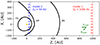 |
Fig. 1. Schematic picture in the BV plane. Models 1 and 2 correspond to the models with Z0 = 1000 AU and Z0 = 50 AU, respectively. The black lines match the discontinuity surfaces from the global heliospheric model. The green arrows show the direction of the plasma velocity and the magnetic field vectors in the undisturbed LISM. |
Many authors successfully applied a Monte Carlo approach for studying the theoretical distribution of ISD grains in the heliosphere (see, e.g., Landgraf 2000; Slavin et al. 2012; Sterken et al. 2012; Strub et al. 2019; Godenko & Izmodenov 2021). The Lagrangian fluid approach based on the Osiptsov method (Osiptsov 2000, 2024) can also be used for modeling (Mishchenko et al. 2020; Godenko & Izmodenov 2023b, 2024), but, for this study, the Monte Carlo approach is more suitable.
3. Results of the modeling
We first demonstrate the effects of the heliospheric interface on the distribution of ISD particles along the trajectory of Ulysses. Figure 2 shows the counts of ISD particles per day obtained by models 1 and 2. The computation results show substantial differences for the smallest (a = 150 nm) grains. In particular, the count values for model 2 are zero for almost the entire mission, while for model 1, there are significant peaks in the middle (∼1997–1998) and close to the end (∼2002–2006) of the mission. Thus, the heliospheric interface facilitates the penetration of particles that are small enough at the heliodistances of the Ulysses orbit (1–5 AU). This somewhat contradicts the concepts that the heliospheric boundaries filter these particles out (Linde & Gombosi 2000; Slavin et al. 2012).
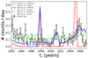 |
Fig. 2. Counts per day on Ulysses for particles of different sizes for the two models with (Z0 = 1000 AU, model 1; solid lines) and without (Z0 = 50 AU, model 2; dotted lines) the heliospheric interface. The different colors match particles of different sizes: a = 150 nm (red lines, β = 1.595), a = 250 nm (blue lines, β = 1.264), and a = 500 nm (green lines, β = 0.639). The black points are the Ulysses experimental counts. |
For the medium-sized grains (a = 250 nm), the corresponding distributions presented in Fig. 2 are similar, but differ noticeably in the middle of the mission (∼1997−1999). For the largest grains (a = 500 nm), the results are almost the same, that is, the heliospheric interface does not influence the trajectories of these particles. We note that the modeled results for medium-sized grains reproduce the Ulysses experimental data well for the second half of the mission (∼1999−2006). In the first half, however, the discrepancies between the modeled and experimental results are substantial. However, the Ulysses experimental counts we present refer to dust grains of all sizes. For a correct comparison with the Ulysses experimental data, the modeling results averaged over the ISD size distribution should therefore be used, but this is beyond the scope of the paper.
The effects of the heliospheric interface are more pronounced for smaller particles because the magnitude of the electromagnetic force, which is dominant in this region, is approximately inversely proportional to the squared radius of the grains. Therefore, the effects of the heliospheric interface are explored below for a = 150 nm dust particles.
To study the differences between the results obtained by models 1 and 2, we considered the distributions of ISD particles in the plane Z = 0, which almost coincides with the plane of the Ulysses trajectory. Figure 3 presents the distributions of the number density for a = 150 nm ISD particles in the plane Z = 0 in 2004 − 2005 obtained by models 1 and 2. The period 2004 − 2005 was chosen because during this period, the differences between the two considered models are greatest.
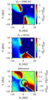 |
Fig. 3. Number density distributions for a = 150 nm ISD particles in the plane Z = 0 in 2004 − 2005. Panels A and B correspond to models 1 and 2, respectively. Panel C shows the difference between the results from panels A and B. The black line matches the Ulysses orbit, and the white segment of the orbit corresponds to 2004 − 2005. |
The distribution in the plane Z = 0 is not homogeneous in either case. The areas of the ISD particle accumulations appear due to specific configurations of the HMF. The magnetic force changes sign at the HCS, and as a result, caustics of the ISD particle trajectories form. The ISD number density increases in the vicinity of these caustics. This effect was discussed by Mishchenko et al. (2020) for the stationary case and by Godenko & Izmodenov (2024) for the nonstationary case. These areas of the ISD accumulation appear in the plane Z = 0 for the two considered models, but the locations, shapes, and sizes of these areas differ significantly. In 2004 − 2005, the Ulysses trajectory crossed the region of increased number density for model 1, but does not do so for model 2. The fact that the Ulysses experimental data also demonstrate an increase of ISD counts during this period could serve as evidence of the heliospheric interface effects.
Inside 50 AU, the two considered models are identical, so that the differences in the ISD distribution may only appear because the ISD flow is modified beyond 50 AU. In the plane Z = 50 AU, outer heliosphere effects may be pronounced in (1) the inhomogeneous distribution of the ISD number density, and (2) deflection of the ISD flow (see Fig. C.1). Additional numerical experiments (see Appendix C) show that the deflection of the ISD flow is the main reason for the significant differences (between the results obtained from models 1 and 2) in the ISD distribution near the Sun that were discussed above. Our numerical calculations show that the velocity deflection mainly appears in the outer heliosheath (between the HP and the BS). In the inner heliosheath, the fast periodic variations in the HMF polarity lead to a fast change in the direction of the electromagnetic force, so that the net effect on the ISD velocity is weak (see, e.g., Fig. 7 from Godenko & Izmodenov 2024).
To explore the ISD velocity deflection in the outer heliosheath, we considered its Y component. Figure 4 demonstrates the evolution of the magnetic field and plasma and dust velocity components along the trajectory of a typical a = 150 nm ISD particle from the plane Z = 1000 AU up to the intersection with the heliopause. The Y-component of electromagnetic force in the LISM is approximately proportional to the following term:
 (2)
(2)
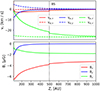 |
Fig. 4. Plasma (solid lines) and dust (dashed lines) velocity (top panel) and magnetic field (bottom panel) components along the trajectory of a typical a = 150 nm dust particle. The left boundary corresponds to the intersection with the heliopause (Z ≈ 112 AU). The vertical dotted black lines match the weak interstellar bow shock. |
because the charge potential U does not change substantially in this region (see, e.g., Kimura & Mann 1998; Godenko & Izmodenov 2023a). The term (vd, x − vp, x)⋅Bz in this expression can be neglected because the Bx component is greater than Bz (in magnitude), and the Z-velocity components (dust and plasma) are greater than the X-velocity components (see Fig. 4). In the undisturbed LISM, the ISD velocity is approximately equal to the plasma velocity, so that Fmag, y ≈ 0. In the outer heliosheath, where plasma decelerates (|vp, z|< |vd, z|), Fmag, y becomes positive, and therefore vd, y increases.
The Bx component is the projection of the magnetic field vector on the axis perpendicular to the upwind direction (in the BV plane), that is, it depends in particular on the angle αBV between the interstellar magnetic field and the plasma velocity vectors. Therefore, the distribution near the Sun could also be sensitive to the parameter αBV.
To verify this hypothesis, we performed computations using the global heliospheric models of Izmodenov & Alexashov (2020) with different values of αBV. Figure 5 presents the computed counts per day on Ulysses for a = 200 nm particles for three different values of αBV: 20°, 40° and 60°. In some segments of the Ulysses trajectory, the differences between the corresponding results are significant. In particular, in the middle of the mission (1997−1998), the peak value of counts for αBV = 60° is four months earlier than for αBV = 20° and 40°. In the second half of the mission, there are some points (≈2001 and 2006) where the quantitative differences of 20 − 30% between the results obtained by the heliospheric models with different values of αBV appear. The described differences are related to the different levels of deflection in the outer heliosheath.
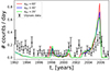 |
Fig. 5. Counts per day on Ulysses for a = 200 nm ISD particles computed with different global heliospheric models. The different colors correspond to different values of αBV in the heliospheric models: (1) 60° (red), (2) 40° (blue), and (3) 20° (green). |
Because the distributions of the ISD particles near the Sun are sensitive to the heliospheric model, the ISD data might therefore potentially be used as a new distant diagnostics of interstellar parameters. The upcoming missions that will study the ISD experimentally, such as Interstellar Mapping and Acceleration Probe (McComas et al. 2018) or Interstellar Probe (Brandt et al. 2023), will open opportunities for using this approach.
4. Conclusions
We have studied the effects of the heliospheric interface on the distribution of ISD particles near the Sun. For this purpose, we developed a Monte Carlo model of the ISD distribution based on the global heliospheric model of Izmodenov & Alexashov (2015, 2020). The conclusions are summarized below:
-
The heliospheric interface strongly modifies the distribution of small enough (a = 150 − 250 nm) astronomical silicates near the Sun but almost does not affect the distribution of larger particles (a = 500 nm). The reason is that the magnitude of the electromagnetic force, which is dominant in the heliospheric interface, is approximately inversely proportional to the squared radius of the grains.
-
The unexpected result is that the heliospheric interface facilitates the penetration of a = 150 nm particles into the inner heliosphere, which somewhat contradicts previous concepts that the heliospheric boundaries filter small dust particles out (Linde & Gombosi 2000; Slavin et al. 2012). The reason for this inconsistency is the fact that our ISD distribution model takes the time-dependent rippled shape of the HCS induced by the 22-year solar cycle and by the 25-day solar rotation into account, in contrast to previous modelers, who only considered the stationary focusing or defocusing configuration of the HMF. Penetrating the heliosphere, in the inner heliosheath, ISD particles move through regions with alternatively changing polarities of the HMF, so that the net effect of the electromagnetic force on the dust particle trajectories is weak. This allows dust grains to move almost freely from the heliopause up to the entrance into the inner heliosphere. Therefore, they are not filtered out at the heliospheric boundaries.
-
The effects of the heliospheric interface are mainly pronounced through the deflection of the ISD flow in the outer heliosheath under the influence of the interstellar magnetic field. For a = 150 nm ISD particles, this deflection reaches 15 − 20% of vLISM in the direction perpendicular to the BV plane. We showed that as a result of this deflection, the ISD particles approach to the Sun more closely, and in particular, cross the Ulysses trajectory. When the deflection in the outer heliosheath is not taken into account, small ISD particles almost entirely miss the Ulysses orbit.
-
The distribution of ISD particles near the Sun is sensitive to the interstellar plasma parameters. This fact provides a new independent approach for distant diagnostics of the LISM and heliospheric boundaries.
Acknowledgments
Authors thank D.B. Alexashov for providing the distributions of plasma parameters from the heliospheric model and discussions.
References
- Alexashov, D. B., Katushkina, O. A., Izmodenov, V. V., & Akaev, P. S. 2016, MNRAS, 458, 2553 [NASA ADS] [CrossRef] [Google Scholar]
- Altobelli, N., Postberg, F., Fiege, K., et al. 2016, Science, 352, 312 [NASA ADS] [CrossRef] [Google Scholar]
- Baranov, V. B., & Malama, Y. G. 1993, J. Geophys. Res., 98, 15157 [NASA ADS] [CrossRef] [Google Scholar]
- Brandt, P. C., Provornikova, E., Bale, S. D., et al. 2023, Space Sci. Rev., 219, 18 [NASA ADS] [CrossRef] [Google Scholar]
- Burlaga, L. F., Ness, N. F., Berdichevsky, D. B., et al. 2022, ApJ, 932, 59 [NASA ADS] [CrossRef] [Google Scholar]
- Burns, J. A., Lamy, P. L., & Soter, S. 1979, Icarus, 40, 1 [Google Scholar]
- Czechowski, A., Strumik, M., Grygorczuk, J., et al. 2010, A&A, 516, A17 [Google Scholar]
- Draine, B. T. 2003, ARA&A, 41, 241 [NASA ADS] [CrossRef] [Google Scholar]
- Godenko, E. A., & Izmodenov, V. V. 2021, Astron. Lett., 47, 50 [NASA ADS] [CrossRef] [Google Scholar]
- Godenko, E. A., & Izmodenov, V. V. 2023a, Adv. Space Res., 72, 5142 [NASA ADS] [CrossRef] [Google Scholar]
- Godenko, E. A., & Izmodenov, V. V. 2023b, Fluid Dyn., 58, 274 [NASA ADS] [CrossRef] [Google Scholar]
- Godenko, E. A., & Izmodenov, V. V. 2024, Fluid Dyn., 59, 521 [Google Scholar]
- Greenberg, J. M., & Li, A. 1996, A&A, 309, 258 [NASA ADS] [Google Scholar]
- Grün, E., Zook, H. A., Baguhl, M., et al. 1993, Nature, 362, 428 [Google Scholar]
- Gustafson, B. A. S. 1994, Annu. Rev. Earth Planet. Sci., 22, 553 [CrossRef] [Google Scholar]
- Hoeksema, J. T. 1995, Space Sci. Rev., 72, 137 [Google Scholar]
- Izmodenov, V. V., & Alexashov, D. B. 2015, ApJS, 220, 32 [NASA ADS] [CrossRef] [Google Scholar]
- Izmodenov, V. V., & Alexashov, D. B. 2020, A&A, 633, L12 [NASA ADS] [CrossRef] [EDP Sciences] [Google Scholar]
- Izmodenov, V. V., & Alexashov, D. B. 2023, MNRAS, 521, 4085 [CrossRef] [Google Scholar]
- Izmodenov, V., Alexashov, D., & Myasnikov, A. 2005, A&A, 437, L35 [NASA ADS] [CrossRef] [EDP Sciences] [Google Scholar]
- Kimura, H., & Mann, I. 1998, ApJ, 499, 454 [Google Scholar]
- Kimura, H., & Mann, I. 1999, in Meteroids 1998, eds. W. J. Baggaley, & V. Porubcan, 283 [Google Scholar]
- Kimura, H., Okamoto, H., & Mukai, T. 2002, Icarus, 157, 349 [NASA ADS] [CrossRef] [Google Scholar]
- Landgraf, M. 2000, J. Geophys. Res., 105, 10303 [NASA ADS] [CrossRef] [Google Scholar]
- Linde, T. J., & Gombosi, T. I. 2000, J. Geophys. Res., 105, 10411 [NASA ADS] [CrossRef] [Google Scholar]
- McComas, D. J., Alexashov, D., Bzowski, M., et al. 2012, Science, 336, 1291 [NASA ADS] [CrossRef] [Google Scholar]
- McComas, D. J., Christian, E. R., Schwadron, N. A., et al. 2018, Space Sci. Rev., 214, 116 [CrossRef] [Google Scholar]
- Mishchenko, A. V., Godenko, E. A., & Izmodenov, V. V. 2020, MNRAS, 491, 2808 [NASA ADS] [Google Scholar]
- Opher, M., Loeb, A., Drake, J., & Toth, G. 2020, Nat. Astron., 4, 675 [NASA ADS] [CrossRef] [Google Scholar]
- Osiptsov, A. N. 2000, Ap&SS, 274, 377 [NASA ADS] [CrossRef] [Google Scholar]
- Osiptsov, A. N. 2024, Fluid Dyn., 59, 1 [CrossRef] [Google Scholar]
- Pogorelov, N. V., Heerikhuisen, J., & Zank, G. P. 2008, ApJ, 675, L41 [NASA ADS] [CrossRef] [Google Scholar]
- Pogorelov, N. V., Fraternale, F., Kim, T. K., Burlaga, L. F., & Gurnett, D. A. 2021, ApJ, 917, L20 [NASA ADS] [CrossRef] [Google Scholar]
- Slavin, J. D., Frisch, P. C., Müller, H.-R., et al. 2012, ApJ, 760, 46 [NASA ADS] [CrossRef] [Google Scholar]
- Sterken, V. J., Altobelli, N., Kempf, S., et al. 2012, A&A, 538, A102 [NASA ADS] [CrossRef] [EDP Sciences] [Google Scholar]
- Sterken, V. J., Strub, P., Krüger, H., von Steiger, R., & Frisch, P. 2015, ApJ, 812, 141 [NASA ADS] [CrossRef] [Google Scholar]
- Strub, P., Krüger, H., & Sterken, V. J. 2015, ApJ, 812, 140 [NASA ADS] [CrossRef] [Google Scholar]
- Strub, P., Sterken, V. J., Soja, R., et al. 2019, A&A, 621, A54 [NASA ADS] [CrossRef] [EDP Sciences] [Google Scholar]
- Tielens, A. G. G. M. 2008, ARA&A, 46, 289 [NASA ADS] [CrossRef] [Google Scholar]
- Wang, S., Li, A., & Jiang, B. W. 2015, ApJ, 811, 38 [NASA ADS] [CrossRef] [Google Scholar]
- Weingartner, J. C., & Draine, B. T. 2001, ApJ, 548, 296 [Google Scholar]
- Witte, M. 2004, A&A, 426, 835 [NASA ADS] [CrossRef] [EDP Sciences] [Google Scholar]
Appendix A: Heliospheric model
As follows from Eq. (1), to compute the trajectories of dust particles in the heliosphere, the distributions of the surrounding plasma velocity vp and magnetic field B vectors should be provided from a model of the global heliosphere. We applied the global heliospheric model of Izmodenov & Alexashov (2015, 2020). The model is based on a self-consistent solution of the ideal MHD equations for plasma particles and the kinetic Boltzmann equation for neutrals. A summary of technical details and boundary conditions used for the heliospheric model can be found in Appendix A of Izmodenov & Alexashov (2020). For computation results presented in our study, the interstellar magnetic field parameters (boundary conditions) were: B = 3.75 μG, αBV = 60°, where αBV is the angle between the interstellar plasma velocity and magnetic field vectors. The only exception is Fig. 5, where the heliospheric models with other boundary conditions were probed.
Figures A.1 and A.2 demonstrate the distributions of plasma parameters (velocity and magnetic field components) from the model with B = 3.75 μG, αBV = 60° along the upwind direction and in the planes Y = 0 and X = 0, correspondingly. One can see that plasma parameters vary substantially in the global heliosphere, especially across the discontinuity surfaces. In particular, near the heliopause, the magnetic field increases in magnitude due to compression of the plasma flow in this region. This pile-up of the magnetic field determines the proposed effects of the heliospheric interface on the motion of charged particles.
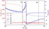 |
Fig. A.1. Plasma parameters (velocity and magnetic field components) distributions along the upwind direction from the heliospheric model. The vertical dotted lines match the location of discontinuity surfaces along the upwind direction. Although the interstellar plasma flow is supersonic (M ≈ 2), the existence of interstellar bow shock has been questioned so far because of the influence of the interstellar magnetic field (see, e.g. Izmodenov et al. 2005; McComas et al. 2012). However, the heliospheric model used provides the weak shock wave in the LISM. |
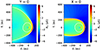 |
Fig. A.2. The Bx component distributions in the plane Y = 0 (left panel) and in the plane X = 0 (right panel) from the heliospheric model. The white lines match the location of discontinuity surfaces (TS and HP) in the corresponding planes. |
It is important to note that a self-consistent solution in the model of Izmodenov & Alexashov (2015, 2020) is obtained in the frame of a “monopole approach” which assumes a single polarity of the HMF in the entire heliosphere. This approach is chosen because the terms responsible for the influence of the magnetic field in the ideal MHD equations do not depend on the orientation of the magnetic field. Therefore, the ideal MHD solution does not depend on the magnetic field polarity. Also, in the frame of the ideal MHD, the HCS is assumed as a discontinuity, where the magnetic field changes its orientation. The structure and width of the HCS are not considered in the heliospheric model. This assumption has been confirmed so far by Voyager magnetic field measurements in the solar wind and in the inner heliosheath (see, e.g., Burlaga et al. 2022) that demonstrate a quick change of the magnetic field orientation rather than a thick (comparing to the size of the heliosheath) transition region.
However, the motion of interstellar dust strongly depends on the polarity of the HMF. In this Letter, we calculate the time evolution of the HCS in the entire heliosphere using the kinematic approach by Czechowski et al. (2010). In the frame of this approach, it is assumed that at the source surface (in our study, the sphere of three solar radii), the HCS is a circle that separates the regions of opposite polarities. Observations show that the inclination of this circle to the solar equatorial plane changes at an approximately constant rate throughout the 22-year solar cycle (Hoeksema 1995). From the source surface, the HCS expands with the solar wind velocity and acquires a rippled shape due to the 25-day solar rotation. To calculate the polarity of the HMF at any given point and moment of time, we trace the trajectory of the solar wind particle from this point and moment of time back to the source surface using the plasma bulk velocity from the global heliospheric model (for details, see Appendix A of Alexashov et al. 2016). Since in the ideal MHD the HMF is frozen into the solar wind plasma, polarity does not change along the solar wind trajectory. At the source surface, the polarity value is determined by the location of the point with respect to the HCS, which is the circle inclined to the solar equatorial plane and turned around the solar rotation axis. The inclination to the solar equatorial plane is obtained from the data of Wilcox Solar Observatory1.
Figure A.3 presents the HCS shape inside the TS in the plane Y = 0 for different moments of time throughout the solar cycle. The HCS in panel A corresponds to focusing configuration of the HMF for positively charged particles because, in this case, the electromagnetic force is directed toward the solar equatorial plane at any point. On the contrary, panel C demonstrates defocusing configuration where the electromagnetic force repels positively charged particles from the solar equatorial plane. In panels B and D, the transition phases of HCS are presented, during which particles move almost along straight lines because the multiple variations of the HMF polarity cancel the effects of electromagnetic force out (see, e.g., Godenko & Izmodenov 2024). Namely, the demonstrated variations of the rotating HCS make the distribution of ISD particles in the heliosphere essentially time-dependent.
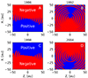 |
Fig. A.3. The HCS shape inside the TS in the plane Y = 0 for different moments of time throughout the solar cycle: 1986 (panel A), 1992 (panel B), 1998 (panel C), 2004 (panel D). The red and blue colored areas match the regions of negative and positive polarities, respectively. The boundary line between the red and blue areas is the HCS. |
After the termination shock, plasma decelerates, and as a result, the unipolar regions of the HMF start to alternatively change even more frequently. Figure A.4 demonstrates the unipolar regions separated by the HCS near the upwind direction in the inner heliosheath (between the TS and HP). When approaching the heliopause, the averaged distance between the consequent regions of the same polarity decreases, and therefore, the HCS loses its rippled structure, and, in particular, the dissipation of the HMF could appear. However, in this Letter, we studied the transport of ISD particles through the HMF, where the proposed dissipation near the heliopause is not considered.
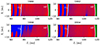 |
Fig. A.4. The unipolar regions of the HMF separated by the HCS in the inner heliosheath near the upwind direction. The white lines match the location of discontinuity surfaces from the heliospheric model. The domination of red colored regions in the inner heliosheath is an optical illusion. Actually, the total sizes of blue and red colored domains are almost the same. |
Thus, the magnetic field used for the modeling of ISD trajectories inside the heliosphere is a product of the corresponding component from the global heliospheric model of Izmodenov & Alexashov (2015, 2020) and the kinematically computed polarity function at the given point and moment of time.
Appendix B: Monte Carlo approach
In this Appendix, we present the details of Monte Carlo computations applied in this study to calculate the ISD distribution in the heliosphere.
We first specify the sampling procedure for the initial coordinates of grains. For each dust grain, we randomly sample the position in the plane Z = Z0, which is determined by two coordinates X0 and Y0, and the moment of time t0 when this particle crosses the plane Z = Z0 (since the electromagnetic force is time-dependent due to the rotating HCS). The coordinates X0 and Y0 are sampled uniformly from the rectangle [Xl, Xr]×[Yl, Yr]. To increase the statistical efficiency of computations, we adjust this rectangle in such a way that it accurately covers the region in the plane Z = Z0 from which the considered particles cross the domain of interest near the Sun. We ensure that the rectangles for different values of Z0 (50 AU and 1000 AU) and for particles of different sizes are located inside the [-70 AU, 70 AU] × [-100 AU, 40 AU] region. Since the electromagnetic force (and, therefore, the ISD distribution) is periodic due to the 22-year solar cycle, t0 can be sampled from any given 22-year period of time [tl, tr]. In this Letter, we use the 22-year period between the two focusing solar minima containing the operational time of the dust sensor on Ulysses: tl = 1986, tr = 2008.
To compute the characteristics of interest (number density, bulk velocity) at the centers of the computational domain cells, we carry out the following procedure N times:
-
In the plane Z = Z0, randomly sample the initial coordinates and the initial moment of time of the particle according to the algorithm described above.
-
Compute the trajectory of a particle numerically solving motion Eq. (1) by the 4-th order Runge-Kutta method.
-
From the computed trajectory, calculate the periods of time tij which this particle spent inside each computational cell (i is the id number of the dust particle, j is the id number of the computational cell). It should be noted that tij = 0 if the i-th particle does not cross the j-th computational cell.
Using the obtained periods of time tij, we calculate the ISD number density at j-th computational cell by the following expression:
 (B.1)
(B.1)
where:
 (B.2)
(B.2)
is the total amount of dust particles entering the computational domain through the rectangle [Xl, Xr]×[Yl, Yr] within the period [tl, tr],  is the ISD number density in the LISM, vLISM is the undisturbed LISM velocity with respect to the Sun (it is assumed, that the velocities of all ISD particles in the plane Z = Z0 are equal to this value), ΔVj = 1 AU × 1 AU × 1 AU × 1 yr is the volume of j-th computational cell. For any considered case, we simulated N = 25 × 106 particles, which allows us to reach the relative statistical uncertainty of 5%.
The components of ISD bulk velocity at j-th computational cell are calculated by the following expressions:
 (B.3)
(B.3)
where vx, ij, vy, ij, vz, ij are the velocity components of the i-th simulated particle when it is inside the j-th computational cell.
To compute counts per day along the Ulysses trajectory (Fig. 2 and 5), we used the obtained values of number density and bulk velocity at the corresponding computational cells containing the Ulysses orbit. The value  km−3 was applied, which provides the modeled counts per day comparable with the Ulysses experimental data, but, actually, the value of
  is uncertain so far. The analysis of Ulysses data provides a way to estimate correctly the value of
  , but it is beyond the scope of the paper.
Appendix C: The effects of the ISD flow modified at 50 AU on the dust distribution near the Sun
In this Appendix, we demonstrate how modifications of ISD distribution in the plane Z = 50 AU influence the ISD distribution near the Sun (in the plane Z = 0). Figure C.1 presents the distributions of number density and velocity components in the plane Z = 50 AU in 1995-1996 obtained from model 1 (Z0 = 1000 AU). The 1995-1996 period in the plane Z = 50 AU was chosen to be in accordance with the 2004-2005 period in the plane Z = 0 because ISD particles require approximately 9 years to cover the distance of 50 AU along the Z-axis direction. One can see that the number density and velocity components are both significantly modified in the heliospheric interface. For model 2 (Z0 = 50 AU), the distributions of number density and velocity components in the plane Z = 50 AU are uniform:  , v/vLISM = (0, −1, 0).
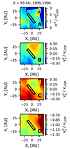 |
Fig. C.1. Number density (panel A) and velocity components (panels B-D) for a = 150 nm ISD particles in the plane Z = 50 AU in 1995 − 1996 obtained from model 1. The black rectangles correspond to the area from where particles cross the area [ − 10 AU, 10 AU]×[−10 AU, 10 AU] in the plane Z = 0. |
We first study the influence of the modified dust number density in the plane Z = 50 AU on the distribution in the plane Z = 0. For this purpose, we consider the motion of particles from the plane Z = 50 AU but take the inhomogeneous distribution of number density into account using the results from model 1 (panel A of Fig. C.1). The velocities of all ISD particles in the plane Z = 50 AU are assumed to be unmodified by the interface (that is, equal to the velocity of undisturbed LISM). Panel A of Fig. C.2 shows the computed number density in the plane Z = 0 in this case of modified number density. Panels B and C demonstrate the differences between the results from panel A and the results obtained by models 2 and 1, respectively. One can see that the results presented in panel A almost do not differ visually from the results obtained by model 2. The reason is that the particles that crossed the plane Z = 0 inside the area shown in Fig. C.2 come from the area in Fig. C.1 where differences in density are not strong. These areas in the plane Z = 50 AU are shown by black rectangles in Figure C.1.
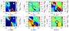 |
Fig. C.2. Number density distributions for a = 150 nm ISD particles in the plane Z = 0 in 2004 − 2005 when we start their motion from the plane Z = 50 AU with the given number density (panel A) or given velocity (panel D) distribution. Panels B and C correspond to the difference between the results from panel A and the results presented in Fig. 3 (models 2 and 1, respectively). Panels E and F show the analogical difference for the results from panel D. |
To study the influence of the ISD velocity deflection, we again consider the motion of ISD particles from the plane Z = 50 AU, but this time take the deflection of the ISD velocity vector into account using the results from model 1 (panels B-D of Fig. C.1). The ISD number density distribution in the plane Z = 50 AU is assumed to be unmodified by the interface (that is, uniform). Panel D of Fig. C.2 shows the computed number density in the plane Z = 0 in this case of modified velocity components. Panels E and F demonstrate the differences between the results from panel D and the results obtained by models 2 and 1, respectively. One can see that the distribution presented in panel D is visually similar to the distribution from model 1. Although there are some regions of nonzero differences, the results of computations show that the deflection of the ISD velocity vector reproduces the main effects of the heliospheric interface on the distribution of ISD grains near the Sun.
To find out how this deflection appears, we consider the evolution of velocity components for a typical a = 150 nm dust particle from the plane Z = 1000 AU up to the Z = 50 AU (Fig. C.3). Outside of BS, the velocity vector of the considered particle experiences visible deflection only along the Y-axis direction, but the deflection is weak (∼2 − 3% of vLISM). In the outer heliosheath (between the HP and BS), the particle starts to significantly deflect. For instance, the magnitude of the Y-velocity component reaches almost 20% of vLISM. Then, after crossing the heliopause (in the inner heliosheath), velocity components start to oscillate around the values reached after the passage through the outer heliosheath due to alternatively changed unipolar regions of the HMF. However, the amplitude of oscillations is relatively small (±5% of vLISM), so namely the deflection of particles in the outer heliosheath mainly produces the resulted deflection of the flow in the plane Z = 50 AU.
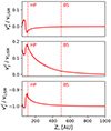 |
Fig. C.3. Velocity components along the trajectory of a typical a = 150 nm particle from the plane Z = 1000 AU up to the intersection with the plane Z = 50 AU. The vertical dotted red lines match the intersections with the heliopause and the weak interstellar bow shock. |
All Figures
|
Fig. 1. Schematic picture in the BV plane. Models 1 and 2 correspond to the models with Z0 = 1000 AU and Z0 = 50 AU, respectively. The black lines match the discontinuity surfaces from the global heliospheric model. The green arrows show the direction of the plasma velocity and the magnetic field vectors in the undisturbed LISM. |
| In the text | |
|
Fig. 2. Counts per day on Ulysses for particles of different sizes for the two models with (Z0 = 1000 AU, model 1; solid lines) and without (Z0 = 50 AU, model 2; dotted lines) the heliospheric interface. The different colors match particles of different sizes: a = 150 nm (red lines, β = 1.595), a = 250 nm (blue lines, β = 1.264), and a = 500 nm (green lines, β = 0.639). The black points are the Ulysses experimental counts. |
| In the text | |
|
Fig. 3. Number density distributions for a = 150 nm ISD particles in the plane Z = 0 in 2004 − 2005. Panels A and B correspond to models 1 and 2, respectively. Panel C shows the difference between the results from panels A and B. The black line matches the Ulysses orbit, and the white segment of the orbit corresponds to 2004 − 2005. |
| In the text | |
|
Fig. 4. Plasma (solid lines) and dust (dashed lines) velocity (top panel) and magnetic field (bottom panel) components along the trajectory of a typical a = 150 nm dust particle. The left boundary corresponds to the intersection with the heliopause (Z ≈ 112 AU). The vertical dotted black lines match the weak interstellar bow shock. |
| In the text | |
|
Fig. 5. Counts per day on Ulysses for a = 200 nm ISD particles computed with different global heliospheric models. The different colors correspond to different values of αBV in the heliospheric models: (1) 60° (red), (2) 40° (blue), and (3) 20° (green). |
| In the text | |
|
Fig. A.1. Plasma parameters (velocity and magnetic field components) distributions along the upwind direction from the heliospheric model. The vertical dotted lines match the location of discontinuity surfaces along the upwind direction. Although the interstellar plasma flow is supersonic (M ≈ 2), the existence of interstellar bow shock has been questioned so far because of the influence of the interstellar magnetic field (see, e.g. Izmodenov et al. 2005; McComas et al. 2012). However, the heliospheric model used provides the weak shock wave in the LISM. |
| In the text | |
|
Fig. A.2. The Bx component distributions in the plane Y = 0 (left panel) and in the plane X = 0 (right panel) from the heliospheric model. The white lines match the location of discontinuity surfaces (TS and HP) in the corresponding planes. |
| In the text | |
|
Fig. A.3. The HCS shape inside the TS in the plane Y = 0 for different moments of time throughout the solar cycle: 1986 (panel A), 1992 (panel B), 1998 (panel C), 2004 (panel D). The red and blue colored areas match the regions of negative and positive polarities, respectively. The boundary line between the red and blue areas is the HCS. |
| In the text | |
|
Fig. A.4. The unipolar regions of the HMF separated by the HCS in the inner heliosheath near the upwind direction. The white lines match the location of discontinuity surfaces from the heliospheric model. The domination of red colored regions in the inner heliosheath is an optical illusion. Actually, the total sizes of blue and red colored domains are almost the same. |
| In the text | |
|
Fig. C.1. Number density (panel A) and velocity components (panels B-D) for a = 150 nm ISD particles in the plane Z = 50 AU in 1995 − 1996 obtained from model 1. The black rectangles correspond to the area from where particles cross the area [ − 10 AU, 10 AU]×[−10 AU, 10 AU] in the plane Z = 0. |
| In the text | |
|
Fig. C.2. Number density distributions for a = 150 nm ISD particles in the plane Z = 0 in 2004 − 2005 when we start their motion from the plane Z = 50 AU with the given number density (panel A) or given velocity (panel D) distribution. Panels B and C correspond to the difference between the results from panel A and the results presented in Fig. 3 (models 2 and 1, respectively). Panels E and F show the analogical difference for the results from panel D. |
| In the text | |
|
Fig. C.3. Velocity components along the trajectory of a typical a = 150 nm particle from the plane Z = 1000 AU up to the intersection with the plane Z = 50 AU. The vertical dotted red lines match the intersections with the heliopause and the weak interstellar bow shock. |
| In the text | |
Current usage metrics show cumulative count of Article Views (full-text article views including HTML views, PDF and ePub downloads, according to the available data) and Abstracts Views on Vision4Press platform.
Data correspond to usage on the plateform after 2015. The current usage metrics is available 48-96 hours after online publication and is updated daily on week days.
Initial download of the metrics may take a while.