| Issue |
A&A
Volume 645, January 2021
|
|
|---|---|---|
| Article Number | A55 | |
| Number of page(s) | 49 | |
| Section | Interstellar and circumstellar matter | |
| DOI | https://doi.org/10.1051/0004-6361/201936534 | |
| Published online | 12 January 2021 | |
Physical properties of the ambient medium and of dense cores in the Perseus star-forming region derived from Herschel Gould Belt Survey observations★,★★
1
INAF – IAPS, Via Fosso del Cavaliere, 100,
00133 Roma, Italy
e-mail: This email address is being protected from spambots. You need JavaScript enabled to view it.
2
Department of Physics and Astronomy, University of Victoria,
Victoria,
BC, V8P 5C2, Canada
3
NRC Herzberg Astronomy and Astrophysics,
5071 West Saanich Road,
Victoria,
BC, V9E 2E7, Canada
4
Instituto de Astrofísica e Ciências do Espaço, Universidade do Porto, CAUP, Rua das Estrelas,
4150-762 Porto, Portugal
5
Department of Physics, Engineering Physics, and Astronomy, Queen’s University,
Kingston, ON K7L 3N6, Canada
6
Laboratoire AIM, CEA/DSM-CNRS-Université Paris Diderot, IRFU/Service d’Astrophysique, CEA Saclay, 91191 Gif-sur-Yvette, France
7
Université de Toulouse, UPS-OMP, IRAP, 31400 Toulouse, France
8
Laboratoire d’Astrophysique de Bordeaux, Univ. Bordeaux, CNRS, B18N, allée G. Saint-Hilaire,
33615 Pessac, France
9
INAF – Osservatorio Astronomico di Roma,
Via di Frascati 33,
00078
Monte Porzio Catone, Italy
10
Dipartimento di Fisica, Università di Roma Tor Vergata, Via della Ricerca Scientifica 1,
00133
Roma, Italy
11
ESO/European Southern Observatory,
Karl-Schwarzschild-Str. 2,
85748 Garching bei Munchen, Germany
12
Jeremiah Horrocks Institute, University of Central Lancashire, Preston, Lancashire PR1 2HE, UK
13
Université Grenoble Alpes, CNRS, Institut de Planétologie et d’Astrophysique de Grenoble,
38000 Grenoble, France
14
Observatorio Astronómico Ramón María Aller, Universidade de Santiago de Compostela,
Santiago de Compostela,
15782
Galiza, Spain
15
Instituto de Matemáticas and Departamento de Matemática Aplicada, Universidade de Santiago de Compostela,
Santiago de Compostela,
15782
Galiza, Spain
16
I. Physik. Institut, University of Cologne, Germany
17
Department of Physics and Astronomy, McMaster University,
Hamilton Ontario L8S 4H7, Canada
Received:
20
August
2019
Accepted:
31
October
2020
Abstract
The complex of star-forming regions in Perseus is one of the most studied due to its proximity (about 300 pc). In addition, its regions show variation in star-formation activity and age, with formation of low-mass and intermediate-mass stars. In this paper, we present analyses of images taken with the Herschel ESA satellite from 70 μm to 500 μm. From these images, we first constructed column density and dust temperature maps. We then identified compact cores in the maps at each wavelength, and characterised the cores using modified blackbody fits to their spectral energy distributions (SEDs): we identified 684 starless cores, of which 199 are bound and potential prestellar cores, and 132 protostars. We also matched the Herschel-identified young stars with Gaia sources to model distance variations across the Perseus cloud. We measure a linear gradient function with right ascension and declination for the entire cloud. This function is the first quantitative attempt to derive the gradient in distance across Perseus, from east to west, in an analytical form. We derived mass and temperature of cores from the SED fits. The core mass function can be modelled with a log-normal distribution that peaks at 0.82 M⊙ suggesting a star formation efficiency of 0.30 for a peak in the system initial mass function of stars at 0.25 M⊙. The high-mass tail can be modelled with a power law of slope ~−2.32, which is close to the Salpeter’s value. We also identify the filamentary structure of Perseus and discuss the relation between filaments and star formation, confirming that stars form preferentially in filaments. We find that the majority of filaments with ongoing star formation are transcritical against their own internal gravity because their linear masses are below the critical limit of 16 M⊙ pc−1 above which we expect filaments to collapse. We find a possible explanation for this result, showing that a filament with a linear mass as low as 8 M⊙ pc−1 can already be unstable. We confirm a linear relationship between star formation efficiency and the slope of dust probability density function, and we find a similar relationship with the core formation efficiency. We derive a lifetime for the prestellar core phase of 1.69 ± 0.52 Myr for the whole Perseus complex but different regions have a wide range in prestellar core fractions, suggesting that star formation began only recently in some clumps. We also derive a free-fall time for prestellar cores of 0.16 Myr.
Key words: stars: formation / circumstellar matter / stars: protostars / dust, extinction / submillimeter: ISM
Full Tables A.1–A.6 are only available at the CDS via anonymous ftp to cdsarc.u-strasbg.fr (130.79.128.5) or via http://cdsarc.u-strasbg.fr/viz-bin/cat/J/A+A/645/A55
Herschel is an ESA space observatory with science instruments provided by European-led Principal Investigator consortia and with important participation from NASA.
© ESO 2021
1 Introduction
The aim of this paper is to derive a catalogue of cold compact cores of condensed dust and gas of ≲0.1 pc in size in the Perseus molecular complex and to present and discuss their physical properties. This work uses Herschel observationsand is part of the Herschel Gould Belt Survey (HGBS, André et al. 2010), which aims to probe the origin of the stellar initial mass function (IMF) by finding the physical mechanisms influencing star formation at its earliest stages. The HGBS team has already published core catalogues for many clouds: Aquila (Könyves et al. 2015, the reference paper for HGBS); L1495 in Taurus (Marsh et al. 2016); Lupus (Benedettini et al. 2018); Corona Australis (Bresnahan et al. 2018); Orion B (Könyves et al. 2020), Ophiuchus (Ladjelate et al. 2020); Cepheus (Di Francesco et al. 2020); and Serpens (Fiorellino et al. 2021).
The analysis of these data has led to the idea that gravitational fragmentation of the cloud filaments is the dominant physical mechanism generating prestellar cores within interstellar filaments (see André et al. 2014, and references therein). It has been suggested inthe past that the filamentary structure of the interstellar medium is fragmenting to form cores (see, e.g. Román-Zúñiga et al. 2009), but only with Herschel did it become clear that filament fragmentation is the dominant mode of (solar-type) star formation, because the physical properties and the spatial distribution of both the diffuse dust and the compact cold cores in the clouds can be derived simultaneously, with sufficiently high spatial resolution, namely of 36′′. Moreover, the large areas observed, combined with the high sensitivity of Herschel instruments, allow the construction of catalogues containing between two and nine times more cores than in previous ground-based surveys (e.g. Johnstone et al. 2000; Stanke et al. 2006; Enoch et al. 2006; Nutter & Ward-Thompson 2007; Alves et al. 2007).
The first prestellar core mass functions (CMFs) in star-forming regions, (e.g. Motte et al. 1998; Testi & Sargent 1998) revealed a similarity between the shape of the CMF and the initial mass function (IMF) of the stars. The system IMF shows (Chabrier 2005) a log-normal distribution with a peak at 0.25 M⊙, and a high-mass tail for M ≥ 1 M⊙ modelled with a power-law function dN∕d log(M) ∝ M−1.35, also known as the Salpeter slope (Salpeter 1955).
A quantitative assessment of the similarity between CMF and IMF was carried out for the Pipe nebula by Alves et al. (2007) who found that the peak of the CMF was about three times higher than the peak of the IMF. Assuming a one-to-one correspondence between cores and stars, the shift in the respective peaks of the CMF and the IMF was interpreted by Alves et al. (2007) as an indication of a star formation efficiency (SFE) per single core of about 0.3, meaning that 30% of the core mass eventually becomes star mass. Later studies confirmed that values around 0.3–0.4 are typical in many other star-forming regions even if different values are also reported (see Sect. 5.1). The similarity between CMF and IMF led to the hypothesis that the IMF is a consequence of the physical mechanisms that produce the prestellar core population. Testing this hypothesis requires derivation of the CMF in many star-forming regions in the most uniform way possible with respect to how observations are executed as well as to how cores are detected and their intensities are measured. Only in this way can the different CMFs be compared consistently (see, e.g. Swift & Beaumont 2010).
Another issue on a proper CMF derivation is that it is very important to assign each core its temperature rather than using a constant temperature for all the cores in a cloud, an assumption that leads to inaccurate core masses. Unless we determine both mass and temperature at the same time, the stability of cores cannot be investigated on a purely photometric basis, and the derived CMF can contain collapsing cores and transient structures that are not forming stars, as pointed out 20 yr ago by Johnstone et al. (2000). Deriving the CMF for the most important nearby star-forming regions in a robust and uniform way is the main aim of the HGBS.
The Gould Belt is a complex of neutral gas and star-forming molecular clouds covering an area of ~ 2.6 × 10⁵ pc2 (e.g. Bobylev 2016); the molecular clouds are located within distances of d≲500 pc of the Sun, which are close enough to observe individual cores. Among them, the system of clouds in Perseus (Fig. 1) are at distances in the range of ~230–320 pc (Hirota et al. 2008, 2011; Strom et al. 1974) with many sites of active low-mass and intermediate-mass star formation. The review by Bally et al. (2008) gives a complete presentation of the region, including its surroundings, with a long list of references; here we limit the literature references to papers that are pertinent to our work or when their results are used in this study.
Perseus was observed as part of the Spitzer Cores to Disks (c2d) program (Evans et al. 2009) with the InfraRed Array Camera(IRAC, Jørgensen et al. 2006) and the Multiband Imaging Photometer (MIPS, Rebull et al. 2007). The analysis of both datasets was later presented by Young et al. (2015). Perseus was also mapped at sub-millimetre (sub-mm) wavelengths with SCUBA (Hatchell et al. 2005) and later with SCUBA-2 (Chen et al. 2016), and at 1.1 mm with BOLOCAM (Enoch et al. 2006).
Examples of previous publications related to HGBS data are the study of B1-E (Sadavoy et al. 2012) and of the relation between Spitzer Class 0 and the distribution of dense gas (Sadavoy et al. 2014, see also Sect. 3.2.4 of this work); Pezzuto et al. (2012) discussed the properties of two sources, B1-bN and B1-bS, that were proposed to be first hydrostatic core candidates (see Sect. 4.3).
The present paper is organised as follows. In Sect. 2, we give an overview of the observations of Perseus and present our data reduction and analysis. In Sect. 3, we derive a first quantitative estimate of the distance gradient across the cloud using Gaia Data Release 2 (DR2) results. We then derive and discuss the column density and temperature maps, and the filamentary structure of the region. In Sect. 4, we present the source extraction and the physical properties of the cores derived via SED fitting. We also discuss the stability of cores against their internal gravity. In Sect. 5, we present the CMF and link the cores to the filaments. We also analyse the core and star formation efficiencies and estimate the lifetimes of the different phases of star formation. In Sect. 6, we summarise our conclusions. We include several appendices with the full source catalogue, completeness testing, region definitions, and the catalogue of sources found in our maps that are not related to star formation, such as galaxies for example.
It is worth concluding this section by introducing some of the terms that are used in the following sections. We define a core as a compact over-density of gas and dust that is round in shape and exceeds the density of its local diffuse background emission appearing as a local maximum in an intensity image or in a column density map. Cores are most easily identified using mid-infrared to mm wavelengths (di Francesco et al. 2007; Ward-Thompson et al. 2007; André et al. 2014).
A core is defined as starless if there is no internal source of energy (e.g. a protostar). Starless cores are instead warmed by the interstellar radiation field and their spectral energy distribution (SED) can be modelled as a single modified blackbody Iν ∝ νβBν(T) at temperatureT. We use our source extraction technique and the modified blackbody fits to derive the radius R, mass M, and temperatureT of the cores, and we use these physical properties to determine the dynamical state of the cores. If the core self-gravity exceeds its pressure support, we consider the source to be bound. We define bound, starless cores as prestellar cores. These objects can collapse, or are collapsing, and will likely form one or more stars. If the self-gravity of a core is insufficient to balance its internal pressure, the core is classified as unbound and may be a transient structure that will dissipate in the future unless it is confined by another mechanism (e.g. pressure confined).
Once a star forms, it warms up the surrounding envelope, whose emission in the first phases still resembles a modified blackbody for λ≳100 μm while at shorter wavelengths the SED is no longer compatible with such a model. For this reason, a core with compact 70 μm emission is considered protostellar because a central source must be present to warm the dust. However, we note that in principle a starless core can be detected at 70 μm if it is sufficiently warm (T≳20 K), and so the shape of the SED at short wavelengths determines if the object is already a protostar. On the other hand, an object undetected at 70 μm is always considered a starless core even if the lack of detection in the PACS band(s) may be just a matter of sensitivity.
The focus of this paper is on starless cores. Protostars are mentioned here when necessary, for instance to derive star formation efficency in Sect. 5.3, but a full discussion on the protostars in Perseus is postponed to a forthcoming paper.
2 Observations and data reduction
Perseus was observed with Herschel (Pilbratt et al. 2010) as part of the HGBS (André et al. 2010) in two overlapping mosaics: the western field (mainly NGC 1333, B1, L1448, L1455) and the eastern field (L1468, IC348, B5). Results from these observations were initially presented in Sadavoy et al. (2012, 2014), Pezzuto et al. (2012), and Zari et al. (2016). Both fields were observed with PACS (Poglitsch et al. 2010) at 70 μm (blue) and 160 μm (red), and with SPIRE (Griffin et al. 2010), at 250 μm (PSW), 350 μm (PMW), and 500 μm (PLW) in parallel mode with the telescope scanning at a speed of 60′′ s−1. The total area common to both instruments is about 13 square degrees. Table 1 gives the observation log.
A composite image using PACS bands and the SPIRE PSW band is shown in Fig. 1. All maps are reported to the same spatial resolution as the 70 μm map by using the method presented in Li Causi et al. (2016).
Each field was observed twice along two almost orthogonal directions to remove better instrumental 1∕f noise. The Herschel raw data were reduced with HIPE (Ott 2010) version 10. For PACS, we reduced the data to Level 1 with HIPE using version 45 of the set of calibration files. Level 1 data consist of the calibrated timelines of the detectors to which the celestial coordinates were added. Afterwards, the data were exported outside HIPE and maps were generated with Unimap (Piazzo et al. 2015) version 6.5.3. The adopted spatial grid is 3′′ and 4′′ for the blue and red bands, respectively.
For SPIRE, we used the calibration files version 10.1 and maps were generated with the destriper module in HIPE. We adopted the default values for the spatial grids: 6′′, 10′′, and 14′′ for PSW, PMW, and PLW bands, respectively. The SPIRE maps are given in Jy beam−1, which we converted to MJy sr−1 using the nominal beamsizes of426 arcsec2, 771 arcsec2, and 1626 arcsec2, respectively. Additional details on the PACS and SPIRE data processing can be found in Könyves et al. (2015).
The alignment of each image was checked by comparing the Herschel position at 70 μm of 22 bright and isolated sources, with their corresponding positions reported in the Spitzer catalogue at 24 μm (Evans et al. 2009), that is, 11 from both the western and eastern parts. For the western field, we found a shift in RA of Δα = 4′′.82 ± 0′′.56 which was added to our coordinates. We also applied a similar shift to the red map. SPIRE maps required no correction. The final residuals in the five maps run from −1/4 of a pixel in the PSW map to +1/5 of a pixel in the red map for right ascension, and from 1/10 of a pixel in the PSW map to 1/3 of a pixel in the blue map for declination.
The PACS and SPIRE maps were made using a common coordinates system, at each band, for both Perseus east and west. A zero-level offset was applied to each map, obtained by correlating the Herschel data with Planck and IRAS data (Bernard et al. 2010). All five maps shown in Appendix D are available on the HGBS archive1.
 |
Fig. 1 Composite image of the star-forming region in Perseus. Blue is PACS 70 μm; green is PACS 160 μm; red is SPIRE250 μm; north is up, east is to the left. The latter two maps have been processed to simulate having the highest resolution of the 70 μm. The resulting image is therefore not meant to be used for scientific analysis. Labels on the map identify the approximate position of main subregions. Monochromatic Herschel intensity maps are reproduced in Appendix D with coordinate grids. |
Log of the observations.
3 Data analysis
3.1 Distance to Perseus
Given that physical parameters such as mass and radius depend on the distance to the sources, we start this section with a discussion on the distance to Perseus. For IC 348, in the eastern part of the complex, Herbig (1998) discussed a variety of distance measurements in the literature and concluded that the value 316 ± 22 pc derived by Strom et al. (1974) is the most reliable. This distance was later confirmed indirectly by Ripepi et al. (2002) who detected δ-Scuti oscillations in one star of IC 348, and concluded that the derived star properties were not compatible with distances ≲260 pc, but were compatible with 316 pc. On the other hand, the western half of the Perseus region is known to be closer, which led to the conclusion that the molecular clouds in Perseus form a chain with increasing distance from west to east (see Černis 1993). This conjecture was definitively confirmed with the measure of maser parallaxes for a couple of sources in NGC 1333 and L1448 (Hirota et al. 2008, 2011) giving a distance of ~ 240 pc.
To gain some insight into this gradient in distance, we exploited the Gaia archive second data release (DR2) of astrometric data (Gaia Collaboration 2016). We looked for sources in our protostar catalogue (see Appendix A) that are spatially close to a source in the Gaia archive with an angular separation of less than 10′′. Objects with negative parallax were excluded. All sources had spatial correspondences of < 8′′, with only two having separations > 6′′ (6.5′′ and 7.4′′). Conversely, 18 are spatially separated by < 2′′ and 7 are separated by < 1′′. Parallaxes were converted into distances following Luri et al. (2018). In particular, we used the DistanceEstimatorApplication.py tool2 with the median of the Exponentially Decreasing Space Density Prior distribution option. The tool also returns the 5% and 95% quantiles that are not symmetrical around the median (this reflects the obvious prior that the distance must be positive). As the difference between the median minus 5% quantile and the 95% quantile minus the median is negligible, we adopted the latter for the distance uncertainty which is slightly larger than the former. No attempt was made to exclude projection effects. Therefore, some associations between our sources and Gaia stars may not be physical. On the other hand, it is unlikely that a proximity of a few arcseconds between a Gaia source at the distance expected for Perseus and a protostar is only due to projection.
In Table 2 we show distances and uncertainties for the 28 sources possibly associated with our protostars. We also report the distances for the maser sources in L1448 (Hirota et al. 2011, h1 in the table) and NGC 1333 (Hirota et al. 2008, h2) derived using the python tool reported above to convert the parallax to distance.
In Fig. 2 the 30 distances are plotted as a function of their right ascension. Starting from the observational finding that a distance gradient exists going from west to east, and noting that a gradient also exists going from south to north (see the different symbols of the points in the figure), we made a multivariate linear fit to the data and found the following relation:
 (1)
(1)
where α0 = 51. °27800 and δ0 = 30. °20121 are the smallest right ascension and declination of sources 1 and 5 in Table 2, respectively. Such a relation, namely d ≡ d(α, δ), is the first quantitative estimate of the distance gradient in Perseus even if the large scatter in distances could be due to false associations between our protostars and Gaia sources. In particular, if all the associations in NGC 1333 are physical, an exceptional depth of more than 100 pc is implied, or an overlap along the line of sight of at least two different clouds (see also Appendix C). Further, there are no data points (no associations) in the range 53. °14 ≤ α ≤55. °20, and so the middle part of the fit is not constrained. A refinement of Eq. (1) will be attempted in a forthcoming paper on protostars, where Class II pre-main sequence stars – which are more easily detected by Gaia – will be distinguished from younger sources, that is, Class 0 objects. The latter, being heavily obscured in the visible light, are more difficult to detect with Gaia and thus an association between a Class 0 source and a Gaia object may be due to a projection effect.
Distance measurements to the main Perseus clouds were recently reported by Zucker et al. (2018) and Ortiz-León et al. (2018). Table 3 compares these distances: column “P” gives the distance based on our Eq. (1) using right ascension and declination from Zucker et al. (2018), column “Z” gives the Zucker et al. (2018) distances, and column “O” gives the Ortiz-León et al. (2018) values. The distances from Zucker et al. (2018) are derived by combining data from PAN-STARRS1, 2MASS, Gaia and the 12CO data from the COMPLETE survey (Ridge et al. 2006a) (we use the 13 CO data in Sect. 3.2.2 and Appendix C). Ortiz-León et al. (2018) measure distances using VLBA and Gaia data. Uncertainties in column P, derived through error propagation from Eq. (1), can be misleading. These are small because they give the (estimated) distance of each point in the sky assuming a 2D geometry for Perseus. These uncertainties do not take into account the dispersion in distance caused by the depth of each cloud, and they do not take into account the fact that there are no protostars in the region with right ascension between ~ 53° and ~ 55°, and therefore we do not have an indication of the distance. Uncertainties in column Z are the sum in quadrature of the random and systematic errors given by Zucker et al. (2018).
We find excellent agreement (<3% differences) between our measurements and those of Zucker et al. (2018) and Ortiz-León et al. (2018). Only IC348 and B5 show more significant differences but still <10% and, in any case, within the uncertainties. Zucker et al. (2019) derived a distance map of Perseus and other molecular clouds through star-specific distance-extinction estimates improved with Gaia parallaxes. The result for a small set of lines of sight is reported in Table 4 where we compare their distances with ours: the agreement is very good, better than 5% in all cases.
The full set of distances derived by Zucker et al. (2019) is shown in Fig. 3 where we give a graphical representation of Eq. (1): our distance was computed for each point of the column density map (see Sect. 3.2) and colour-coded according to the bar on the right of the figure. Zucker et al. (2019) give the distance averaged over boxes of 0.84 deg2, and these are shown in green at the position of the centre of each box in Fig. 3.
While Zucker et al. (2019) computed accurate distances to Perseus that are more precise than those given by our Eq. (1), it is nevertheless not easy to extract a distance for a given point in space from their map; for instance, B5 is seen to be at 302 pc in Zucker et al. (2018), a distance that can hardly be derived from the grid of distances shown in Fig. 3. Conversely, our Eq. (1) has been derived in a less rigorous way, but it immediately gives a reference distance at any point (α, δ) in space, a distance that captures the distance gradient in the complex, and closely matches the distances derived by other authors.
For the rest of the paper, we adopted the mean of the 30 sources, 300 pc, as a representative value of the distance for the whole Perseus complex (294 pc in Zucker et al. 2019). However, below we show how the physical description of the whole region changes when distances are varied according to our formula.
Sources from our protostar catalogue with a Gaia counterpart within 10′′.
Comparison between distances, in pc, derived by different author.
Comparison between the distance, in parsecs, derived in this paper (column P) and that derived by Zucker et al. (2019) (column Z) for the four lines of sight reported in their Table 3 for the Perseus cloud.
3.2 Dust temperature and column density maps
Dust emission in the far-infrared can be modelled as a modified blackbody Iν = κνΣBν(Td), where κν is the dust opacity per unit mass expressed as a power law normalised to the value κ0 at a reference frequency ν0, such that  cm2 g−1. Here, Σ is the gas surface-density distribution
  with
with  being the molecular weight, mH the mass of the hydrogen atom, and N(H2) the column density assuming the gas is fully molecular hydrogen. Finally, Bν (Td) is the Planck function at the dust temperature Td. Following the conventions of the HGBS (Könyves et al. 2015), we adopted an opacity of 0.1 cm2g−1 at 300 μm (gas-to-dust ratio of 100), a dust opacity index β = 2, and
  representing the mean weight per hydrogen molecule (Kauffmann et al. 2008).
We used the four intensity maps from 160 μm to 500 μm to derive N(H2) and Td maps. The 70 μm map was not included because emission at this wavelength may include contributions from very small grains (VSGs), which cannot be modelled with a simple single-temperature modified blackbody. Indeed, Schnee et al. (2008) found that in Perseus contribution from VSGs may elevate the 70 μm emission by 70% at 17 K and by 90% below 14 K. Contribution from VSGs is not expected for λ > 100 μm (Li & Draine 2001).
The three intensity maps shortwards of 500 μm were degraded to the spatial resolution of the PLW band (36′′. 1), and then the four maps were regridded onto a common coordinate system using 14′′ pixels at all wavelengths.
The SED fitting procedure was executed pixel by pixel with a code that takes the four images in FITS format as input. The code creates a grid of models, as in Pezzuto et al. (2012), by varying only the temperature in the range 5 ≤ Td(K) ≤ 50 in steps of 0.01 K. For each temperature Tj, the code computes the intensity at far-infrared wavelengths for a fixed column density of 1 cm−2.
As Iν is linear with N(H2), we can compute the column density at each pixel using a straightforward application of the least-squares technique,
 (2)
(2)
where fi is the observed SED Iν at each frequency i, and qi (Tj) is the synthetic SED model at frequency i and temperature Tj. The uncertainty σi is 10 and 20% for SPIRE and PACS respectively (Könyves et al. 2015). Index i runs from 1 to 4, index j runs from 1 to 4501, which is the number of models in the grid.
At each pixel of the intensities maps, the model j with the smallest residuals is kept as the best-fit model. To be consistent with the other HGBS papers, we ran the code without applying colour corrections but in Sect. 3.2.2 we show how much the results depend on this assumption and on the choice of β = 2. The code, available on request, outputs the column density map, the temperature map, and the map of the uncertainty of N(H2).
Another column density map at higher spatial resolution (i.e. 18′′. 2 corresponding to the SPIRE 250 μm band) was also obtained using the method described in Palmeirim et al. (2013). The procedure is based on a multi-scale decomposition technique. The high-resolution column density map used to optimise the source extraction described in Sect. 4.1 is available for download from the HGBS website. This map, shown in Appendix D, has a higher spatial resolution than those previously obtained with the same Herschel data at 36′′. 1 (Sadavoy et al. 2014; Zari et al. 2016).
The column density and temperature maps of Perseus at the PLW spatial resolution are shown in the two panels of Fig. 4. The top panel shows the column density map and the bottom panel shows the temperature map. Contour levels in the column density map are 3 × 1021 cm−2 and 1022 cm−2. The first level follows the border of the known main regions relatively well, even if B3 and B4 form a single complex with IC348, while the other marks the densest part of the clouds.
The histogram of Td is shown in Fig. 5. There are two peaks seen at 16.4 K and 17.1 K, and a third, very broad one, indeed a plateau, at 19.2 K. The first two peaks correspond to the temperatures of the diffuse medium in west and east Perseus, respectively. In other words, the dust temperature is slightly lower in the western half of Perseus than in the eastern half. The peak at19.2 K reflects the inner parts of NGC 1333 and IC 348, and a few other regions that we discuss below.
To checkour results, we compared the Herschel N(H2) map with the all-sky Planck map of the optical depth τP at 850 μm (Planck Collaboration XI 2014)3. First we convolved our map to the Planck resolution of 5′ and projected the result onto the Planck grid. We then computed the ratio r = τH∕τP where  . Because of the convolution, the Herschel column density and, as a consequence, the optical depth, have very low values close to map borders, with τH as low as 6 × 10⁻²¹. To exclude these points, we made the comparison in the region where τH ≥ 1.38 × 10−5 = min(τP).
In Fig. 6 we show the ratio r versus τP; we also highlight the small values of r corresponding to τH < 1.38 × 10⁻⁵ (green points). The blue histogram shows the mean ratios, averaged in bins of 10−4, excluding the green points. The weighed mean of the histogram values is  . The blue points are compatible with a constant ratio for r. On the other hand, an increasing trend of r with τP seems present in the figure, with r≲1.05 for τP < 3 × 10⁻⁴, and increasing up to 1.30 when τP ~ 8 × 10⁻⁴. In particular, 98% of the points of the optical depth map have 1.38 × 10⁻⁵ ≤ τP ≤ 3 × 10⁻⁴, and for them the ratio r is 1.05 ± 0.15. A change in r might be evidence of a change in opacity at high column density.
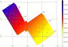 |
Fig. 3 Color-coded 2D visualisation of Eq. (1). Color bar is in parsec, coordinates grid in degrees. Black dashed lines connect points at the same distance, shown in the labels. The coordinates grid, in blue, is in steps of 2°. Green labels are the distances derived by Zucker et al. (2019) in boxes of 0.84 |

3.2.1 Possible contribution of very small grains
As written, the 70 μm map was not used to derive the column density map, because of possible VSG emission at this wavelength. However, we can estimate this contribution by computing the intensity map at 70 μm from the column density and temperature maps obtained for λ ≥ 160 μm. Figure 7 compares the extrapolated 70 μm map with the difference map between the extrapolated and observed data. All maps have been convolved to 36′′. 1 resolution. The most striking feature of Fig. 7 is that the dense subregions in Perseus are expected to be dark against the brighter diffuse background emission if observed with an instrument of high-enough sensitivity. Such 70 μm dark clouds are typically classified as infrared dark clouds (IRDCs, Carey et al. 1998). However, the observed data (see Appendix D) do not show the subregions as silhouettes.
The right panel of Fig. 7 shows the difference between the observed 70 μm map, degraded in spatial resolution and projected onto the 500 μm spatial grid, and the computed 70 μm map. If the far-infrared dust emission can be extrapolated by a modified blackbody distribution, then the difference map should approach zero everywhere. This is indeed true for most of Perseus with the exception of NGC 1333 and the complex IC348/B3/B4/L1468, with differences as high as 103 MJy sr−1 in NGC 1333.
As a first hypothesis we suppose that there is not a population of VSGs and that the differences in observed and computed 70 μm flux are due to poor estimation of Td. In fact, for a modified blackbody, T, β, and the wavelength where the SED peaks λpeak are related through the relation (Elia & Pezzuto 2016)
 (3)
(3)
If T = 18.7 K, the SED peaks at λpeak = 160 μm if β = 2. At higher temperatures, λpeak moves shortwards of 160 μm, meaning that the peak wavelength, and therefore T, is poorly determined from our dataset built for λ ≥ 160 μm. To quantify this effect, we derived the column density and temperature maps using only PACS data. To this aim we used an additional PACS intensity map at 100 μm, also observed as part of the HGBS and that will be the subject of a future paper focused on Class 0 objects.
The 70 μm and 100 μm maps were degraded to the red band spatial resolution, projected onto the spatial grid of the latter image, and then fitted following the same pixel-by-pixel technique described previously. As the 100 μm observation covered a smaller area than the PACS/SPIRE parallel-mode observations, and because the PACS intensities have larger uncertainties in the zero-level of the diffuse emission, the resulting N(H2) and T maps offer less coverage and higher noise when compared to the “nominal” maps obtained for λ ≥ 160 μm.
The new temperature map, TPACSonly, was then degraded to the 500 μm spatial resolution and projected onto the spatial grid of the nominal T map, T160+SPIRE. Figure 8 shows the mean of the ratio TPACSonly∕T160+SPIRE as a function of TPACSonly in bins of 1° K. At low temperatures, TPACSonly is a poor estimate of T, as expected. However, the trend for TPACSonly > 20 K is more interesting. In this regime, corresponding to λpeak≲150 μm, the peak of the SED falls outside the range of wavelengths used to derive T160+SPIRE. On the other hand, the PACS bands span the SED peak, making TPACSonly a more reliable measurement of the dust temperature, at least as long as T≲43 K (above this temperature the SED peak moves at λ < 70 μm). From the figure, we see that T160+SPIRE starts being colder than TPACSonly for T > 20 K (for TPACSonly > 28 K, the value of the mean is likely affected by the small number of points).
The blue contours in the right panel of Fig. 7 show the regions where TPACSonly ≥ 20 K. These regions are confined to the inner parts of IC348 and NGC 1333. Clearly, underestimation of Td cannot explain the large difference where the observed emission at 70 μm is higher than that computed from the 160 + SPIRE column density and temperature maps. The VSG population in Perseus may be the cause ofthis excess. However, if so, it is clear that VSGs are detected primarily in the eastern field. We also note that the bubble CPS5 (Arce et al. 2011), for which Ridge et al. (2006b) derived T ~29 K with IRAS 60 and 100 μm data, is notvisible in the right panel of Fig. 7, suggesting that its 70 μm emission seen by Herschel is, rather, compatible with a modified blackbody at lower temperatures, that is, those less than ~20 K. HD 278942, thought to be the driving source of the bubble, has a distance of ~520 pc (Gaia Collaboration 2016), excluding that this star can indeed be related to the shell.
The factthat T can be underestimated when T > 20 K could in principle have an impact on the core temperature derived from SED fits when a source is not visible in the PACS blue band. However, for the starless cores, almost all of their temperatures are <20 K with only a few exceptions. Sources with temperatures >20 K are detected at 70 μm, meaning that the observed SED covers the region of the peak intensity.
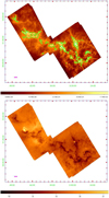 |
Fig. 4 Top panel: column density map with contours at 3 × 1021 cm−2 and 1022 cm−2. Bottom panel: dust temperature map. In both panels, the magenta line in the bottom-left corner shows the angular scale corresponding to 1 pc at 300 pc; J2000.0 coordinates grid is shown. Both maps have a spatial resolution of 36′′. 1. The anticorrelation between N(H2) and Td is evident: regions at high/low column density are cold/warm, with few exceptions in IC348 and NGC 1333. |
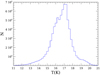 |
Fig. 5 Histogram of dust temperature in the range 11–21 K (minimum is 10.1 K, maximum is 28.3 K). |
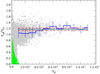 |
Fig. 6 Ratio of τH, the optical depth derived from our Herschel observations, to τP, the opticaldepth derived from Planck observations (Planck Collaboration XI 2014) (grey points), with both τ values computed at 850 μm. The ratio is plotted vs. τP. Green pointscorrespond to low values of τH due to the convolution applied to the Herschel column density map (see text). Mean values ± one standard deviation of the grey points, excluding the green ones, are shown with the blue histogram. The dark green and the two red lines show the weighted mean of the ratio: 1.174 ± 0.040. |
3.2.2 Masses and temperatures of the Perseus subclouds
From the intensity maps at the different wavelengths or the column density map, it is not clear how to define the borders of individual subregions of Perseus. The contour at 3 × 1021 cm−2 shown in Fig. 4 provides a good first-order estimate of the dense material, but it does not separate the individual subregions well. Further, our choice of 3 × 1021 cm−2 does not have a physical meaning and it may be possible to adopt another level of N(H2) and measure a different mass.
To find a solution for the border definition, we started drawing a polygon enclosing each 3 × 1021 cm−2 contour. Indeed, a polygon is much easier to handle in a computer code given the fact that it is defined with much fewer vertices. We therefore used such polygons to obtain a first guess for the borders. Then we visualised the 13 CO 1–0 (Ridge et al. 2006a) spectrum inside each area, the perimeters of which were varied manually to find locations with one velocity component. However, this approach was only possible in a few cases because most of regions have multiple CO components. In the end, we therefore defined the different subclouds in an attempt to obtain one bright line with few contaminants. The areas thus defined are shown in Fig. 9 while in Figs. C.1 and C.2 they are overplotted onto the 13 CO intensity maps at different velocity components to make it clear why a certain region was defined with that border. We introduced additional zones not associated with already known subregions, naming them HPZ#, that is, Herschel Perseus Zone number #. In Appendix C we also give the coordinates of the corners for all regions in DS9 format.
In Table 5 we report the main physical properties of each identified subregion. Columns labelled RA and Dec give, in degrees, the position of the peak in column density reported in the fourth column (for HPZ1, the peak is located on the far-east side of the subregion, and so we computed the geometrical centroid of the zone). In the next columns we give mass, area, and median temperature for the whole region and within the denser part where N(H2) > 3 × 1021 cm−2. The last twocolumns show the effect of assigning a different distance to each point of the column density map, following Eq. (1). Specifically, Md(α,δ) shows how the total mass of the cloud is affected, and column “ ” gives the distance at which
  , where
  , with i running over all the pixels of each subregion. The total mass, area, median temperature, and the mean distance for the entire cloud within specific column density ranges are given in Table 6. From the values of
  in this table we conclude that our choice of 300 pc as representative distance is reasonable.
The mass for N(H2) > 1 × 1022 cm−2 is 954 M⊙ at 300 pc. With the same set of data, Sadavoy et al. (2014) found 1171 M⊙ when adopting 235 pc, which translates into 1908 M⊙ at our distance of 300 pc, a factor of two higher than our value. The main difference between the two analyses is that we adopted a newer version of the calibration files with slightly different SPIRE beamsizes. As the mass enclosed within a certain contour scales with the area defined by that contour, small variations in column density can cause large variations in mass. In particular, scaling the column density derived by Sadavoy et al. (2014) by 30%, the area decreases from 600 arcmin2 to 303 arcmin2 and the mass reduces to 944 M⊙, in agreement with the values we derive.
We also compare the Herschel-derived column density maps with the near-infrared extinction maps based on star counts (see, e.g. Cambrésy 1999; Schneider et al. 2011). However, such a comparison is not immediate. Benedettini et al. (2015) found large discrepancies between the masses derived in Lupus with these two methods, which they attributed to uncertainties on the opacity law used to compute the Herschel column density map. The situation is more difficult for Perseus because of the known variability of R ≡AV∕E(B − V). Foster et al. (2013) found a strong correlation between R and AV in Perseus, with the former increasing from ~3 to ~5 when the latter goes from 2 to 10 mag. Without a priori knowledge of the relation R = R(AV), it is not possible to translate N(H2) to AV. Moreover, AV maps are also subject to a zero-level uncertainty, in the sense that stars must be counted relative to a fiducial zone where AV = 0 mag. As Perseus is a large cloud, it is difficult to find such a clean region.
To investigate further, we derived the mass enclosed within a certain contour of AV using both our column density map and a 2MASS-based extinction map (Cambrésy 2015, priv. comm.), taking into account the different spatial resolution and pixel size. We use the nominal conversion N(H2) = 9.4 × 10²⁰AV mag−1 cm−2 from Bohlin et al. (1978), which assumes fully ionised hydrogen and R = 3.1. The mass found for AV > 3 mag is 3620 M⊙ in our map and 9980 M⊙ in the extinction map, a factor 2.76 higher. However, for AV > 5 mag, the ratio decreases to 2.35 (1830 M⊙ and 4290 M⊙). The comparison improves if we derive the mass enclosed within the same area instead of the same AV. The area is found projecting the AV contour derived on the extinction map onto our column density map. In this way, we measure in our map 5523 M⊙ and 2548 M⊙ for AV > 3 mag and 5 mag, respectively, with a ratio mass(extinction map)/mass(column density map) of 1.81 and 1.68 for the two contours. A qualitatively similar trend is found in Orion B (Könyves et al. 2020). Overall, the masses derived from our Herschel-based column density map are accurate to within a factor of ~ 1.5−2 for AV > 3 mag. At low column densities, AV < 3 mag, we may overestimate the dust opacity and consequently underestimate the masses by a factor of ~ 2−3 (Benedettini et al. 2015).
To test the hypothesis that R can play a role in causing column density discrepancies, we varied R until good agreement was found between the extinction map and the thermal dust map. We chose a fiducial extinction level of AV = 7 mag to make this comparison, so that any uncertainties in both maps from the zero-point corrections are negligible relative to the measured column of dust. We then searched iteratively for the value of R that equalises the masses found from the two maps. We find a best match for R = 3.95 which implies N(H2) = 7.34 × 10²⁰AV mag−1 cm−2. With this conversion, the cloud mass for AV > 7 mag is roughly 1600 M⊙ from both maps. Assuming the nominal value R = 3.1, the thermal dust map gives a mass of 1213 M⊙ and the extinction map gives 2046 M⊙.
Another study of the extinction in the Perseus molecular cloud has been done by Zari et al. (2016) using the same set of Herschel images. These latter authors give the mass enclosed within a set of AK contours based on the relation AK = 1.67 × 10²²[2N(H2) + N(H)] mag cm−2, which becomes AK = 8.35 × 10²¹ N(H2) mag cm−2 assuming fully molecular hydrogen. To take into account the different mean molecular weight (1.37 × 2 instead of our value 2.8) and the different adopted distance (240 pc instead of 300 pc), we increased their masses by 1.53.
Finally, we had to consider the different dust opacity, which was more difficult. By combining Eq. (9) from Zari et al. (2016), namely the relation between AK and N(H2), with Eq. (4) from the same paper, which relates AK with the optical depth at 850 μm, we derived
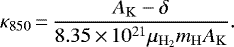 (4)
(4)
The fact that in the above equation the zero-point δ is not zero makes κ850 a function of AK; on the other hand, if AK ≫∥δ∥ = 0.05 mag, then κ850 → 0.0065 cm2 g−1. As we have assumed a dust opacity index β = 2, κ300 = 0.052 cm2 g−1. Also, because Iν ∝ κνΣ, lowering κν by a factor 0.052∕.1 = 0.52 implies increasing our values of N(H2) by the factor 1∕0.52 = 1.92.
We downloaded the τ850 map of Zari et al. (2016) from the CDS and converted it into AK following their prescription. Our N(H2) was projected onto that of Zari et al. (2016) in order to take into account the different pixel size, and then we computed the mass enclosed within the AK contours used by Zari et al. (2016). For AK > 0.2 mag, the ratio between the mass MZ derived by Zari et al. (2016) and the mass estimated from our column density map, MP, is 1.72 instead of the expected value of 1.92. This small difference of 10% in mass could be due to the different way in which the zero-level of the intensity maps is derived, combined with the fact that for 0.6 mag, the zero-point δ in Eq. (4) is not yet negligible. The ratio of the masses increases with increasing AK until, for AK > 6.4 mag, it reaches 1.93, as expected.
We finish this section by showing how the mass derived from the intensity maps depends on the spatial resolution of the column density map, on the dust opacity index β fixed to a value of 2, and on the fact that colour corrections are neglected. In Table 7, we report the masses enclosed within different N(H2) levels and for AV > 7 mag converted into column density values using R = 3.1. The first set of columns show the masses from our data for β = 2 and the second set show our data for β = 1.7, which is the peak of the distribution of β in the Perseus region (Planck Collaboration XI 2014). For each β case, we measure masses before (No CC) and after applying a colour correction (see below for details). Finally, in the middle column for the β = 2 set, we also give the mass when the column densities are convolved to the Planck resolution (5′) with a 90′′ pixel size.
In general, smoothing the map decreases the column density in the densest parts and increases the column density in the more diffuse regions surrounding the denser material. For example, at N(H2) > 1022 cm−2, we recover only 62% of the mass measured in the smoothed Herschel map at 5′ resolution compared to the original map at 36′′ resolution, whereas for N(H2) < 3 × 1021 cm−2, we find a slightly higher mass in the 5′ resolution map. With β = 1.7, the column density and cloud mass decreases substantially. We find values that are roughly 75–80% of what was obtained with β = 2.
Table 7 shows that the colour corrections (CC) decrease the estimated masses by 70–90%. Such corrections are in general necessary because the flux calibration of PACS and SPIRE was performed assuming that the SED of a source displays a flat νFν spectrum4. For all other kinds of SEDs, the derived fluxes must be colour-corrected according to the intrinsic source spectrum. To compute the column density with colour corrections applied, our fitting code integrates the synthetic SEDs over the PACS and SPIRE response filters during the generation of the grid. In this way, each model has its own CC built in. In the remainder of this paper, we use the maps at the spatial resolution of 500 μm derived as in the other HGBS works: no CC applied and β fixed to a value of 2.
 |
Fig. 7 Left panel: inferred 70 μm intensity map extrapolated from the column density and temperature maps obtained for λ ≥ 160 μm. The green circle shows the bubble found by Ridge et al. (2006b) (CPS5 in the list by Arce et al. 2011). Right panel: difference between the observed 70 μm map and the extrapolated map. Green contours are 20 and 200 MJy sr−1; blue contours show the region where TPACSonly ≥ 20 K (see text). Colour bars are in MJy sr−1. |
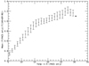 |
Fig. 8 Change in dust temperature when only PACS data are used (70, 100 and 160 μm) instead of PACS 160 μm plus SPIRE bands. Error bars are one standard deviation. The point at T ~ 30 K is not reliable because only a few values are available to compute the mean. |
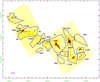 |
Fig. 9 Regions identified in Perseus overplotted on the column density map. The magenta line in the bottom left corner shows the angular scale corresponding to 1 pc at 300 pc. The J2000.0 coordinates grid is also shown. Coordinates of the regions are given in Appendix C. |
Properties of the sub-regions of the Perseus molecular cloud.
Properties of the Perseus molecular cloud as a whole in three different regimes of column density.
Mass cloud derived with two dust emissivity indices β, without and with colour corrections applied, and with a different spatial sampling of the column density map.
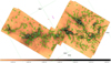 |
Fig. 10 Network of filaments overplotted on the column density map. Red lines show the spine of the filaments, white lines show the branches, and the green contours show the width of the filaments and branches. The map has been rotated by 28°. The magenta line in the centre shows the angular scale corresponding to 1 pc at 300 pc. The J2000.0 coordinates grid is shown. |
3.2.3 Filamentary structure of Perseus
One of the main results of Herschel in the field of star formation is the discovery of the deep link between the filamentary structure of molecular clouds and the sites where stars form. In particular, star-forming cores are found preferentially in denser filaments (André et al. 2010; Molinari et al. 2010; Rayner et al. 2017).
Based on Herschel data, Polychroni et al. (2013) derived two distinct core mass functions in L1641, part of the Orion A complex, forsources inside and outside of filaments. The mass distribution of the sources on the filaments was found to peak at 4 M⊙ with a CMF at higher masses modelled with a power law dN∕d logM ∝ M−1.4. The mass distribution of the off-filament sources has a peak at 0.8 M⊙ and a flat CMF at masses lower than ~4 M⊙.
Roy et al. (2015) found a possible link between the 1D power spectrum of filaments and the origin of the high-mass tail in the core mass function (very close to the Salpeter law dN∕dM ∝ M−2.5).
A complete study of the filaments in Perseus is not within the scope of this paper; nevertheless, given the aforementioned results, it is important to give here at least a short summary of the main properties of the filaments, which are discussed in Sect. 5 where the relation with the core population is addressed.
We used the filament-detection algorithm5 of Schisano et al. (2020, 2014) to identify filamentary structures and their properties across our column density map. Here we summarise how the algorithm works, adopting the nomenclature described in those papers.
By thresholding the minimum eigenvalue of the Hessian of the column density map, the code is able to find and encompass regions where there are maximum variations of the contrast, that is, the bright features on the map. Filamentary structures are picked among these features through selection criteria on the elongation and coverage of the regions of interest. Once the regions of interest are identified, the IDL6 morphological operator “THIN” is applied to them. The result of the operator is the “skeleton” region. Because of the nested morphology of filamentary features, the skeleton in each region is composed by one or more “branches”. The spine of the filament is defined as the group of consecutive branches, which are connected to each other and trace the longest possible path over the filamentary region.
Schisano et al. (2014) found that the area of the filament is underestimated by a mere thresholding of the eigenvalue, which only traces where the emission is concave downwards. These latter authors also found that by enlarging the border by three pixels in both directions perpendicular to the spine gives a better estimate of the position where filaments merge with the background. We verified that such an approach is valid also for our case and we applied it to our filament sample.
The code was run on the 36′′-resolution column density map. Among the identified features, we selected as filaments the elongated regions having a spine longer than 12 pixels, corresponding to 0.24 at 300 pc, or about four times the spatial resolution at 500 μm.
The result of the extraction is shown in Fig. 10 where the filaments are overlapped on the column density map. Green lines show the filament borders, and red and white lines are the spines and the branches, respectively.
In the left panel of Fig. 11 we show the details of all the features previously defined: the filament border (thin grey line), the main spine (white line), and the system of branches (short black lines), for the case of the L1448 cloud. The identified filament runs along almost the entire cloud. The thick black line defines an arbitrary region R used in the right panel of Fig. 11 to show the radial profile of the filament, averaged along the filament itself, and to assess, at least in one case, the validity of the three-pixel border expansion.
The filament-detection code expands the filament border radially by three pixels to identify the positionwhere the filament merges with the surroundings. The average radial profile inside R is shown in the right panel of Fig. 11. The error bars are the standard deviation of the column density for each bin of distance from the spine. Because of the irregular shape of expansion, which reflects the irregular filament profile, the border does not have a constant offset from the spine. The minimum and the maximum radial distance from the spine reached by the filament border over R, r1 and r2, respectively, are shown with thin black lines, running parallel to the spine, in the left panel of Fig. 11. For distances |r| ≤ r1, within the two vertical dashed black lines in the right panel of Fig. 11, all the pixels of the map belong to the filament area, while for distances |r|≥ r2, marked with the two dotted black lines, all the pixels are external to the filament which contains only background pixels. At intermediate distances r1 ≤|r|≤ r2, to be part of the filament or not becomes a local property, depending on the position along the spine.
The background is estimated from linear interpolation of the pixels that are outside the filament area, where |r| ≥ r2, or locally where r1 ≤|r|≤ r2. This estimated background is shown with a thick grey line in the right panel of Fig. 11. The blue line in the same figure is the Gaussian fit to the radial profile. The filament width is estimated as the FWHM of the fit. The Gaussian fit gives another estimate of the background, but we prefer to use the linear interpolation because the Gaussian fit is less suited to catching possible asymmetries, as is visible in our example. These asymmetries are stronger in the wings of the profile than in the inner part, meaning that it is reasonable to use the Gaussian FWHM to estimate the width.
In Fig. 12 we show the filament widths averaged over the spine and deconvolved by the FWHM at 500 μm, 36′′. The width is given in parsecs assuming a distance of 300 pc. The peak of the distribution is ~ 0.08 pc, consistent with the finding of Arzoumanian et al. (2019) of a characteristic width of 0.10 ± 0.03 pc for the filaments in eight HGBS regions.
An important physical parameter for filaments is the mass per unit length. Theoretical models of isothermal infinite cylindrical filaments confined by the external pressure of the ambient medium predict the existence of a maximum equilibrium value to the mass per unit length (Ostriker 1964):
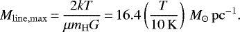 (5)
(5)
Above this value the filament is unstable and can fragment to form cores.
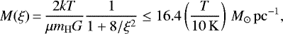
In our case, Mline = M∕L where the mass M of the filament is μmH ∑ini(H2)A with A the area of one pixel in cm2, and the sum is over all the pixels in the filament area, while L is the spine length. We note that A depends on the distance as d2 while L depends on d, and so M∕L increases with d, and, for a constant d = 300 pc, is likely overestimated in the western half of Perseus, and underestimated in the eastern half.
In Fig. 13 we show the distribution of the mass per unit length for all the filaments we find in Perseus that contain at least one core of any type (for core definition and extraction, see Sect. 4.1 below). The mass per unit length distribution peaks at ~ 1.7 M⊙ pc−1, well below the typical value of 16 M⊙ pc−1 of Eq. (5). If we consider that 10 K is not representative of the dust temperature and that we should adopt T≳12 K (see Fig. 5; see also Arzoumanian et al. 2019, where a range between 11 and 30 K is found for the dust temperature of filaments in many HGBS regions) the peak in the distribution is more than a factor of ten smaller than the maximum linear mass.
An important issue here is the background subtraction because, if the background is overestimated, the linear mass of the filament is underestimated. To address this problem we made use of the results found by Hacar et al. (2017). They derive 14 kinematically coherent structures in NGC 1333 through observations of the N2 H+ (1–0) line. These structures, named fibres, are similar to what we call branches. However, the comparison between fibres and branches is not easy because of the different tracers used (molecular gas vs. dust emission), and because of the different algorithm used to derive the structures. Only in one case did we find a fibre and a branch that have a reasonable spatial overlap with a similar length. This happens for fibre number 9: Hacar et al. (2017) derived a length of 0.47 pc and Mlin = 58.5 M⊙ pc−1, while we find a length of 0.50 pc and Mlin = 62.5 M⊙ pc−1, and so, at least for this case, the background estimate appears to be reliable.
As only prestellar cores are likely star-forming in nature (see Sect. 4.3), it is perhaps more reasonable to consider the filaments that contain prestellar cores instead of the filaments that contain only unbound cores. In this case (blue histogram in Fig. 13), the peak of the distribution increases to ~ 7 M⊙ pc−1. This value isstill less than the value Mlin∕Mlin,max. Adding the candidate prestellar cores (see again Sect. 4.3) to enlarge the samples of bound cores changes the shape of thehistogram (dashed red line), but only in the region of smaller masses. In any case, the majority of filaments are below Mlin,max. However, we note that Fischera & Martin (2012) found that fragmentation and core formation can occur in filaments when Mlin∕Mlin,max > 0.5, that is, close to our value.
Similarly, Benedettini et al. (2018) found that the majority of filaments with bound cores in Lupus have Mlin < Mlin,max. These latter authors suggest that the mass per unit length of a filament should be considered locally instead of giving one value for a whole filament. Indeed, if we compute Mlin for the single branches instead of considering the entire filament, we derive a much broader distribution toward high values, ≳130 M⊙ pc−1, of Mlin. Nonetheless, the median of the distribution is ~ 1.5 M⊙ pc−1 with a peak at less than 1 M⊙ pc−1.
Nevertheless, we note that the formula given in Eq. (5) gives the maximum line mass for isothermal equilibrium when the non-dimensional radius ξ of a filament goes to infinity. However, in the more general case of finite ξ, Eq. (5) reads (Ostriker 1964)
 (6)
(6)
where the equality holds only for ξ →∞. Therefore, in the more general case of finite ξ, the mass M(ξ) of a self-gravitating cylinder in thermal equilibrium is smaller than the asymptotic Mlin,max for the same temperature.
The non-dimensional radius ξ can be transformed back to a physical radius once we know T and ρ0, the temperature and central density of the filament, respectively. Alternatively, one can estimate ρ0 from the observed values. For example, if we assume T = 16 K and Mlin,max = 8 M⊙ pc−1, Eq. (6) solved for ξ gives ξ ~ 2.15. Subsequently, if we assume 0.08 pc to be the typical filament radius, solving Eq. (45) in Ostriker (1964) for the central density yields ρ0 ~ 4.3 × 10⁻²⁰ g cm−3 or n0 ~ 9 × 103 cm−3 for μ = 2.8. Strictly speaking, 0.08 pc is the width of the filament, defined as the FWHM of the Gaussian fit. If instead we define the radius as 1.29 × FWHM (Pezzuto et al. 2012), then the typical filament radius becomes ~0.10 pc and n0 ~ 5.5 × 103 cm−3. In any case, we conclude that as long as n≳n0, a filament with radius 0.08 pc and T = 16 K has Mlin,max = 8 M⊙ pc−1, similar to the peak value we find in the histogram of Fig. 13.
 |
Fig. 11 Left panel: zoom-in of the filament in the region of L1448. The white line is the spine, while the grey line is the border of the filament. The short black lines are branches. To explain how the radial profile of the filament is derived, we defined, with the thick black line, an arbitrary region. Right panel: radial profile of the filament averaged longitudinally within the black region shown in the left panel. The error bars are the standard deviation of the column density averaged within ten pixels. The blue line is the Gaussian fit, and the grey line the estimated background. The dashed and dotted vertical lines are explained in the text. |
 |
Fig. 12 Histogram of the filament widths averaged over the spine (bin size 1 pixel or 0.02 pc at d = 300 pc). |
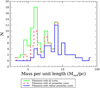 |
Fig. 13 Histograms of mass per unit length for filaments with cores (green line) and prestellar cores (blue and red lines, see text). |
3.2.4 The probability density function of the column density map
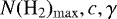
The probability density function (PDF) derived from the column density map has previously been used to probe the physics governing the diffuse medium (see Schneider et al. 2015, for a review on PDF). Briefly, the PDF shows a log-normal behaviour at low densities due to the turbulence in the cloud, while a power-law tail develops at higher densities as a consequence of self-gravity and star-formation activity.
In Fig. 14, we present the PDF for the whole molecular cloud. We model the observed distribution with log-normal and power-law functions, fitting each curve independently. The brown line shows the best log-normal fit to the low-column density part of the distribution. The peak is at N(H2) = (9.738 ± 0.061) × 1020 cm−2. However, the significance of this fit is limited by the fact that the smallest value for column density with a closed contour in our map is N(H2) ~ 1.6 × 1021 cm−2. As a consequence, the shape of the PDF in the region where the log-normal fit is derived can be distorted by incompleteness in the data (Alves et al. 2017 argued that the overall log-normal shape is created rather than distorted by incompleteness).
Moving now to the high-column-density tail in the PDF, Federrath & Klessen (2013) showed that the following relation exists between s, the power-law slope in the PDF, and q, the power-law slope ρ(r) ∝ r−q of the volume density for cores:
 (7)
(7)
meaning that if s is derived, information can be obtained on how the star-formation process in a cloud is proceeding.
To find the exponent of a power law, the easiest and most often used solution is to linearise the problem in log-log space, obtaining an equation of the kind logy = logc − γlogx. The unknowns c and γ are immediately found by fitting a straight line to the dataset. Nevertheless, this procedure should be avoided for many reasons (Bauke 2007; Clauset et al. 2009); for instance, it violates the assumption that uncertainties on the dependent variable follow a Gaussian distribution. This assumption is the basis for a least-square fit.
Our strategy instead was to directly fit a function y = cxγ using a non-linear fitting routine. We used the linearisation scheme described above to obtain only a first estimate of the parameters. As we do not know the extent of the interval over which the fit should be applied, we treated the interval extremes,  and
and  , as free parameters.
In this way, it is not possible to directly compare the χ2 corresponding to each model, because the number of data points is not constant. Furthermore, the use of the reduced χ2 with non-linear models is questionable because the degrees of freedom in this case are generally not known7. To derive the best model we adopted the cross-validation method (Andrae et al. 2010). Namely, for a given  and
and  , we computed the best c, γ excluding one point of the dataset, and from the derived best-fit model we computed the difference between the expected value and the model-derived value. This procedure is repeated for all the points in the dataset and the product of all the differences gives an estimate of the likelihood for that model. We then looked for the maximum likelihood value among all the models (
 ,
, ).
).
The validity of this strategy is limited by the fact that the PDF often does not show a clear power-law trend. As a consequence, the fit procedure tends to minimise the interval  –
– . To impose physical constraints on the fit, we varied
  around the value reported in column “N(H2)” of Table 10, which is discussed below. This value in column density is the smallest background column density8 found for prestellar cores in each sub-cloud. As the power-law tail should trace the region where gravity is strong enough for cores to form, it seems reasonable to impose that
  is not much different from the minimum background column density.
To derive an uncertainty for  and
and  , dubbed x1 and x2 in Fig. 14, we created the PDF histogram with five different bin sizes from 0.8 to 1.2, in steps of 0.1, in units of 1020 cm−2 (the one shown in the figure corresponds to the choice 1 × 1020 cm−2). The power-law slopes and limits were found for the five histograms and similar solutions were sought. The red line in Fig. 14 shows the power-law whose slope is the weighted average of the five slopes and is measured over an interval of 7.935 × 10²¹ and 1.54 × 1022 cm−2. These intervals are the mean of the five starting and end points over which the fit extends.
For the whole Perseus cloud, the minimum background column density for prestellar cores is 9.4 × 1020 cm−2 (see Table 10). We were not able to find any good power-law fit starting from such small values. Indeed, the best fit we found (slope –3.190) is limited to 7.9 × 1021 cm−2 but it is nonetheless a good solution down to ~ 4 × 1021 cm−2, as can be seen from the green line that extends the best fit to smaller column densities.
Our slope − 3.190 ± 0.033 is in good agreement with the value –3 found by Zari et al. (2016), and translates into q = 1.6269 ± 0.0065, similar to the 1.5 slope expected for spherically symmetric free-fall collapse. According to Schneider et al. (2015), this slope should be relatively insensitive to the spatial resolution and to the histogram bin size.
Sadavoy et al. (2014) found a correlation between the slope of the PDFs and the star formation efficiency. We discuss this topic below. Here, we show the results for the individual subregions defined in Fig. 9. Figure 15 shows the PDFs for each of the subregions that hosts at least one protostar. In many cases, the low-density portion cannot be fit with a log-normal function, while the high-density tail shows a wide range of values (labels s in Fig. 15). The slopes s for the single clouds are different from the one found for the whole Perseus region, as predicted by Chen et al. (2018). Through Eq. (7), the interval in slopes translates into an interval for q, limited by 1.5 in IC348, and by 2.3 in HPZ6 (however, for this region the result of the fit is not meaningful).
It is notpossible to directly compare our slopes with those found by Sadavoy et al. (2014), given the different strategy adopted. To make the comparison, we derived the slope of the power law following the method of these latter authors: first, we fixed  to 7 × 1021 cm−2, which is 30% (see Sect. 3.2.2) of 1 × 1022 cm−2, the value adopted by Sadavoy et al. Second, we made a linear fit in the log-log plane. The slopes are compared in Table 8.
In this table we report both the slopes found with our data according to the procedure written above (column P) and the slopes found with our data but following the same procedure as in Sadavoy et al. (2014) (column PS). Naming the values reported in columns S and PS, s ± σs and p ± σp, respectively, we see that s > p always. In three cases s − σs < p < s and in another three case the intervals s − σs and p + σp overlap. Only for L1448 do we find a difference that is slightly larger than 1σs, namely p = s− 1.4σs. We conclude that the slopes reported in Fig. 15 differ from those reported in Sadavoy et al. (2014) because of the different strategy adopted to fit the power-law tail in the PDF. When used in the rest of this paper, the slopes of the PDFs are those reported in Fig. 15.
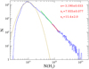 |
Fig. 14 Column density PDF for the whole Perseus molecular cloud: s is the slope of the power-law fit, shown in red, over the interval x1–x2, both in 1021 cm−2. As shown with the green line, the fit can be extended down to ~4 × 1021 cm−2. The brownline is a log-normal fit to the low-density PDF whose parameters are given in the text. Note that N(H2) ~ 1.6 × 1021 cm−2 is the smallest column density having a closed contour in our map. |
 |
Fig. 15 Probability density functions for the subregions identified in Perseus where protostars were detected. In each panel, s gives the slope of the power-law fit, shown in red, in the interval delimited by x1 and x2, both in 1021 cm−2; the fitting procedure is detailed in the text. The x-axis is N(H2) in cm−2. Green lines extend the best fit over the interval of column densities where protostars were found (see Col. N(H2) in Table 9). |
4 Physical properties of the cores
4.1 Source extraction
Sources were extracted from the intensity images using release 1.140127 of getsources (Men’shchikov et al. 2012; Men’shchikov 2013), a multi-scale, multi-wavelength source-extraction algorithm. Its application to the fields of the HGBS is described in Könyves et al. (2015). We followed their strategy to detect starless cores and protostars by running getsources twice with two separate sets of parameters to optimise the extraction. In the following we summarise the extraction procedure.
For starless cores, we extracted sources on the SPIRE intensity maps and the high-spatial-resolution column density map (Palmeirim et al. 2013, see also Sect. 3.2). We also use the 160 μm data via a temperature-corrected map, which is obtained by convolving the PACS red image to the resolution of the SPIRE 250 μm band and then combining them to derive a two-colour column density map (Könyves et al. 2015). The purpose of this approach is to avoid strong gradients of intensity that can be found in proximity to photon-dominated regions or hot sources. For protostars, only the 70 μm band was used for detection.
After source detection is completed, flux intensity, or simply flux, is measured for each source by getsources at all Herschel wavelengths. In particular, at 160 μm we use the intensity map, and not the colour-corrected map which is only used for detection. To both catalogues, we applied the selection criteria used for Aquila (Könyves et al. 2015). Starless cores were selected using the following criteria:
-
column density detection significance greater than 5;
-
global detection significance over all wavelengths greater than 10;
-
global “goodness” ≥ 1;
-
column density measurement with S/N greater than 1 in the high-resolution column density map;
-
monochromatic detection significance greater than 5 in at least two bands between 160 μm and 500 μm;
-
flux measurement with S∕N >1 in at least one band between 160 μm and 500 μm for which the monochromatic detection significance is simultaneously greater than 5.
Prostostars were selected using the following criteria:
-
monochromatic detection significance greater than 5 in the 70 μm band;
-
positive peak and integrated flux densities at 70 μm;
-
global “goodness” ≥ 1;
-
flux measurement with S∕N > 1.5 in the 70 μm band;
-
FWHM source size at 70 μm smaller than 1.5 times the 70 μm beam size (i.e., <12′′.6);
-
estimated source elongation <1.30 at 70 μm.
The two catalogues were cross-matched to look for associations within 6′′. We found 60 sources present in both catalogues. These sources were removed from the core analysis, as they are considered as candidate protostars. In Appendix A we explain in more detail how the SEDs were built for the objects detected in both catalogues. Sources with no counterpart at 70 μm were classified as tentative starless cores. We then visually inspected the intensity maps and column density map toward each candidate to be sure that the source is not an artefact. This step removes non-existent sources due to local fluctuations in the maps and also finds candidate protostars present only in the starless cores catalogue (e.g. protostars that are not well detected at 70 μm). The reason for this depends on the slightly different criteria used to build the catalogues (see Appendix A for details). To remove known galaxies we queried the NED9 and SIMBAD10 archives.
Starless cores not visible at 70 μm but with a SIMBAD counterpart at shorter wavelengths were removed from the catalogue because starless cores are not expected to be detected ≲160 μm. We use a distance criterion of 6′′. As the association with a SIMBAD source may be only spatial and not physical when a starless core with no detection at 70 μm also has a submm counterpart within 6′′ beside a counterpart at short wavelengths, the source was left in our catalogue.
We also scanned the WISE11 (Wright et al. 2010) archive within a radius of 6′′ from our objects, requiring a S/N greater than 0 in bands 3 and 4. This approach is relatively conservative because the threshold of S/N is very low. Moreover, there remains the possibility that two different sources appear close to each other in projection. In any case, sources with a WISE counterpart were removed. All the starless cores removed from our catalogue are reported in Appendix E.
In the end, we were left with 816 candidates: 684 starless cores and 132 protostars. A search for counterparts within 6′′ in the c2d archive (Evans et al. 2009)12 shows no associations for the starless cores, while about 70% of our prostostars have a possible counterpart. The catalogue, presented in Appendix A and available at the CDS, reports data for all 816 sources, both starless cores and protostars. In the following we discuss the physical properties of the starless cores while the protostars will be the subject of a forthcoming paper.
As an additional check on the reliability of the detected sources, we made a second extraction with a completely different source-identification algorithm, namely CuTEx (Molinari et al. 2011). This method identifies sources via second-order differentiation of the signal image in four different directions, looking for minima of the curvature. Since CuTEx makes detection and measurements on single band images, it is not straightforward to make comparisons with extractions by getsources, which builds its catalogue by combining the results of monochromatic detections. Given that the peak of the SED of cold cores is expected around 250 μm, we looked for agreement between getsources and PSW CuTEx catalogues. Indeed, we find that 467 (68%) of getsources cores have a CuTEx-detected object located within the 250 μm elliptical extent measured by getsources.
We find excellent agreement (98%) between the protostar catalogues derived with getsources and CuTEx. As both algorithms use only the 70 μm data to extract the candidate protostars, where diffuse emission is less intense, it is not surprising that the two methods find similar objects.
Comparison of the PDF power-law slopes found by Sadavoy et al. (2014) (column S) and in this paper (column P).
4.2 SED fitting
Once the source catalogue had been produced, we fitted the measured SEDs using a grid of theoretical models. This approach, already used in Benedettini et al. (2018) and equivalent to that used in Sect. 3.2, consists of generating a number of modified blackbodies
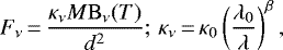 (8)
(8)
where M is the mass of the isothermal emitting dusty envelope at temperature T and distance d. For the dust opacity, we used the same parametrisation as for the column density map: κ0 = 0.1 cm2g−1 at λ0 = 300 μm with β = 2.
The grid of models was constructed fixing M = 1 M⊙ and d = 1 pc, while T was varied in the range 5–50 K in steps of 0.01 K (4501 models). The distance is scaled to the required value, namely of 300 pc for Perseus, during the fitting procedure.
Using a grid instead of a non-linear fitting procedure confers two advantages. First, it is not necessary to give initial guesses of the parameters, which are more or less arbitrary. Second, as long as the grid is large and dense, we can be sure to find the global minimum and not a local one.
As Eq. (8) is linear in M, the mass can be found with straightforward application of the least squares method when comparing a given SED to the grid of models, as shown in Eq. (2). Among the 4501 models, the best fit corresponds to the pair (T, M) with the minimum χ2. Uncertainty on T is derived considering all the models that have  (Andrae 2010). Then, if T1 and T2 are minimum and maximum temperatures of these models we give
  .
.
Uncertainty in M was derived both according to the least squares method, and from the variation in mass corresponding to T1 and T2. Clearly, if T1 < T2 then M2 < M1. The larger of thetwo uncertainties was then adopted.
The fitting procedure was not applied for SEDs with less than three significant flux measurements (see Appendix A). We also did not look for the best fit in cases where Fν (350 μm) < Fν(500 μm). For all these cases, we adopted a fiducial temperature equal to 10.4 ± 1.0 K, the median temperature of all the reliable SEDs, excluding the protostars. The uncertainty on this median is arbitrarily large (the median ΔT∕T for reliable sources is ~3%). For these sources, the mass was computed from the measured integrated flux density at the longest significant wavelength, assuming T = 10.4 K. The numberof sources with reliable SEDs is 519 cores and 85 protostars. However, for the latter Eq. (8) is not an appropriate model, even if it can provide an estimate of the envelope properties. As noted earlier, discussion of the protostars catalogue is beyond the scope of this paper.
4.3 Core classification and stability
As explained in Sect. 4.1, we classify a core as protostellar if it is in emission at 70 μm. This approach is physically plausible because in general cold cores are not visible at this wavelength, often not even at 160 μm. On the contrary, once the source isvisible at 70 μm, a star has already formed, warming up its surrounding envelope. However, this rule does not always apply. In principle, all cores emit in the PACS bands, and their detection at 70 μm depends on its physical properties combined with the sensitivity of the instrument. Indeed, we find seven objects (ID #48, 692, 745, 754, 756, 761, 769 in the catalogue) with 70 μm emission that is either uncertain or at a level compatible with or below the best-fit SED found with Eq. (8). These sources were classified post facto as starless cores.
First hydrostatic cores (FHSC) are expected to have excess 70 μm with respect to a modified blackbody, even if they cannot be considered genuine Class 0 objects. They have masses comparable to those of giant planets and radii of only a few astronomical units (Larson 1969). Source #500 is indeed such a candidate (B1-bS, Pezzuto et al. 2012). However, in our catalogue we classified this source as a protostar because its properties are not compatible with those of the starless cores.
Finally, source #777 was first classified as starless because its 70 μm emission was an upper limit. From visual inspection this source is visible at 70 μm, but as the uncertainty on the flux is higher than the flux itself, the code used to make the SED fitting classified it as starless, putting an upper limit on the blue band. We re-define this source as a protostar.
Among the starless sources, we want to identify cores that are not stable against their own gravity. As a result, they are likely to be collapsing or on the verge of collapse, forming one or more stars in the near future. As in other HGBS studies (e.g. Könyves et al. 2015), we adopted the Bonnor-Ebert (BE) critical mass as an indicator of the maximum mass a core can have whilst remaining stable against gravitational collapse. For an isothermal sphere consisting of particles of mass m, the BE mass is (Bonnor 1956):
 (9)
(9)
where μ = 2.33 is the mean molecular weight per free particle (Kauffmann et al. 2008), RBE is the BE radius estimated as the deconvolved geometrical mean radius of each source measured in the high-resolution column density map, k is the Boltzmann constant, and G is the gravitational constant. We imposed a deconvolved radius of 6′′.1, which is one-third of the FWHM at 250 μm, to sources that are unresolved. We note that in the above equation, non-thermal effects like turbulence or magnetic fields are not taken into account. If the source mass is M, we define an object as bound (or prestellar) if it has MBE,crit∕M ≡ αBE ≤ 2 (see Könyves et al. 2015). We also note that in the catalogue tables presented in Appendix A, we used the short name prestellar for bound cores and starless for unbound cores, even if both are starless, for consistency with the other HGBS catalogues.
For unresolved cores, the deconvolved radius tends to zero, causing MBE,crit → 0, and therefore Könyves et al. (2015) used a set of simulated bound cores to find that bound, unresolved cores can be identified if  , where FWHM is the non-deconvolved source radius estimated in the high-resolution column density map and HPBW is the linear map resolution, 18′′.2. Sources that fulfilled this criterion were named candidate bound cores while cores with αBE ≤ 2 were named robust. In this paper we adopt the same nomenclature.
We simulated bound cores as in Könyves et al. (2015) to derive the completeness limit in mass of our survey. In Appendix B we present our simulations. We find that, for sources with masses greater than ~ 0.32 M⊙, our survey is complete at ≳90% in general, but this limit depends on the contrast between source intensity and background level. We also used the simulations to verify that the above formula for candidate bound cores also works in our case.
4.4 Mass, temperature, and radius
Figure 16 shows the relationship between mass and radius for the whole population of 519 cores. At any radius, bound cores are more massive than unbound cores: this is not a consequence of using Eq. (9) as the stability criterion. A massive starless core can be unbound if sufficiently warm and, conversely, a low-mass starless core can be bound if sufficiently cold. The fact that bound cores are more massive implies some relation between M and T, an anticorrelation that is in fact present in our data (see below Fig. 18).
For the population of unbound cores, we find M ∝ R1.28, shown with the red line in Fig. 16, while for candidate bound cores, we find M ∝ R1.32, the solid black line in the same figure. Bound cores do not show a clear relation between mass and radius: indeed, the best-fit slope is M ∝ R0.25. The lack of correlation is not surprising given that: (i) Eq. (9) is a relation between mass, temperature, and radius. When, as in our case, T is not assumed constant, as it generally was before Herschel, there is not an obvious relation between M and R; (ii) If a bound core is collapsing, it is not even expected to be described by Eq. (9). In fact, our stability criterion is not that M is equal to MBE, but rather that M is greater than MBE by some factor. Coming back to the original paper by Bonnor, in particular the plot p − V in Fig. 1 of Bonnor (1956), bound cores should populate the curve on the left of point A, where instability is dominating. Equation (9) of the present article, on the contrary, describes the condition of a core that is found exactly on point A.
In Fig. 16 the dashed blue line shows the M− R relation for cores at T = 6.7 K with αBE = 2. This temperature is the lowestwe derived for prestellar cores. We consider this line to be the lower-limit for bound cores in our sample. However, we note that for T = 6.7 K and β = 2, the modified black body distribution peaks at λ > 430 μm, which means that we may lack colder, bound cores in our data because we imposed that Fν (350 μm) > Fν(500 μm) in Sect. 4.2.
The smallest radius in our sample, 0.0089 pc or 6′′.1 at 300 pc, simply reflects our choice to impose a deconvolved radius of one third of the FWHM at 250 μm to sources that are unresolved. The largest observed radius is 0.11 pc for bound cores. During the detection and measurement of the sources with getsources, we imposed a maximum radius of 220′′ (0.32 pc), which is three to four times larger than the largest core size that we detect. Therefore, this size constraint does not affect our results. Instead, we find that the cores in Perseus have a maximum size of ~ 0.1 pc. This limiting size could be physical or may reflect another, unaccounted for bias. For instance, larger cores may have smaller density contrasts between their peaks and the background, which makes them more difficult to detect.
In Fig. 17 we show the relation between the temperature T of the cores and their mean column density N(H2) (defined as M∕πR2, where T, M, and R are derived from source SED fitting). We modelled the trend seen with the equation T = slogN(H2) + b. Two different slopes are found for prestellar and unbound cores: − 1.27 ± 0.21 and − 4.32 ± 0.41 for bound and unbound, respectively. This result is in contrast with what was found by Marsh et al. (2016) in L1495. These latter authors found that the trend from the unbound populations continues smoothly when entering thebound region, with a single slope being enough to describe the overall trend. Their slope itself, of − 3.6, is different from the value of − 4.32 we find for unbound cores. Such a difference could be due to the different environments in which cores are embedded.
In deriving the M − T slope for the unbound cores, we excluded seven objects that are clearly warmer than other cores, namely those with T >20 K. Including these points gives s = −5.43 ± 0.67. These sources are the seven starless cores that show emission at 70 μm (see Sect. 4.3). As noted earlier, detection in the PACS blue band does not necessarily mean that a source has evolved into a protostar. In fact, a starless core with T >20 K has the peak of the SED approaching the PACS blue band (λ < 144 μm for β = 2, Elia & Pezzuto 2016) while at low T the peak moves at longer wavelengths so that the emission at 70 μm becomes too faint to be detected. Moreover, the SED increases at higher T as L ∝ T4+β (see Elia & Pezzuto 2016). In principle, one could have bright enough starless core emission at 70 μm by also increasing the mass, but the intensity depends only linearly on M, meaning that huge masses are required to make an unbound and cold core visible at short λ. The seven sources described here are warm and have small masses (see black triangles in Fig. 17).
In principle, there is no reason why warm unbound cores should not exist. However, their position in Fig. 17 seems to define a class of sources that are independent from the other unbound cores. It is possible that these sources have poorly determined intensities, which means that T was not estimated correctly. For example, they could be objects falling very close to strong sources, meaning that their envelope is unusually warm. Alternatively, these sources could have some intrinsic properties that make them different from the others. As our goal here is a statistical description of the cold core population in Perseus, we do not further investigate this small sample.
Finally, in Fig. 18 we show the relationship between M and T, which shows similar distinctions between the populations to those seen in Fig. 17. The anticorrelation between M and T is evident (see the discussion about Fig. 16).
For anygiven temperature, there is a mass below which cores are not detected. To investigate this phenomenon from a quantitative point of view, we studied whether or not, and to what extent, the sensitivity of the Herschel instruments plays any role. First we constructed a SED with the SPIRE-PACS Parallel Mode 1-σ instrument sensitivity for a point source13 divided by  because of the two directions. The sensitivities are then 14.8 and 33.2 mJy for PACS, and 8.91, 7.42, and 10.6 mJy for SPIRE. We then made a fit to this SED with the same routine and grid of models used for the detected cores, and the same distance of 300 pc. The best fit model has T = 23.9 K and M = 1.7 × 10⁻⁴ M⊙. For each T, we then derived the mass that scales the model to the SED of sensitivities. For instance, at 20 K the mass is M = 3.4 × 10⁻⁴ M⊙, at 10 K M = 5.3 × 10⁻³ M⊙, and so on. Clearly, the match between models and sensitivity-based SED is increasingly poor as T decreases, but to first approximation, and without considering measurement uncertainties, these values give an estimate of the smallest detectable mass for a given T compatible with Herschel sensitivities.
All these values give the magenta line in Fig. 18, which is accurately described by M ∝ T−4. This line, derived from Herschel sensitivities for a point source, can be considered as the locus of the smallest detectable mass of a compact source as a function of temperature. The line is well below the detected masses: indeed, in star forming regions it is well known that the Herschel detection of cores is not driven by the sensitivity but by the contrast between core and diffuse medium emission. Interestingly, a simple scaling by the arbitrary factor of 15, which was found by eye, gives the black line that accurately reproduces the smallest detected mass of starless cores for T≳8 K.
We can see that for T≲9 K, unbound cores are not detected; indeed, the minimum temperature in our catalogue for an unbound core is 9.5 K. This could be an observational bias, because at low temperatures, MBE decreases while the smallest detectable mass of a source increases. Therefore, an unbound cold core must have high mass to be detected and large radius so as not to be unbound, but low T and high R equate to a faint and diffuse object that could remain undetected.
The magenta line does not work with bound cores for T≲8 K. The smallest detected mass scales as T−12.2, shown in Fig. 18 with a red line. This slope was found by choosing two arbitrary bound cores by eye, with T = 8.9 K and M = 0.13 M⊙, and with T = 7.2 K, M = 1.73 M⊙. A possible explanation for this behaviour is based on the finding that more massive prestellar cores are found in regions of high column density (see Fig. 21 in Sect. 5.2). As a consequence, a bound core is detected if massive enough to show up against the bright diffuse medium, and the minimum mass no longer reflects the law M ∝ T−4 which is more related to the instrument sensitivity. This conclusion is consistent with the result shown in Appendix sectionlinking B.2 where we discuss the completeness in mass.
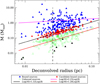 |
Fig. 16 Relation between mass and radius for all the 519 detected cores: vertical dashed line corresponds to 0.026 pc, the linear distance corresponding to the FWHM (18′′. 2) of the high-resolution column density map at 300 pc. The three power laws are fit to our data. Black triangles are hot starless cores discussed in the text; also the blue dashed line is discussed in the text. |
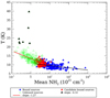 |
Fig. 17 Relation between T and mean column density of the sources, where symbols are defined as in the previous figure. The two lines are linear fits of the form T = slogN(H2) + b. The slopes s are given inthe legend and in the text where we also report the uncertainties. Black triangles are hot starless cores discussed in the text. |
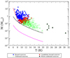 |
Fig. 18 Relation between T and M of the sources. The warmest unbound source at ~40 K is not shown to limit the extension of the x-axis. Bound sources are shown in blue, unbound sources in green, and candidate bound sources in red. |
5 Discussion
5.1 Core mass function
The histograms in Fig. 19 show the CMFs for robust prestellar cores (blue line), and for robust and candidate prestellar cores (red line) in Perseus in the form dN/d logM. The histograms use logarithmic bin sizes of 0.1. The most massive candidate prestellar core has M = 1.24 M⊙, meaning that blue and red lines overlap at high masses.
The results found by Swift & Beaumont (2010) show that with 199 sources it is difficult to discern between a power-law tail and a log-normal to model the CMF shape. Therefore, we separately fit both a power law and a log-normal function to the CMF shown in Fig. 19.
The high-mass tail was fit with a power law for M > 1 M⊙. Given the limited number of sources, the size of the bin of the histogram may play a role. We therefore followed the prescription of Maíz Apellániz & Úbeda (2005) and used a variable bin size with a fixed number of values in each bin. In this procedure, N values, here representing the core masses, are arranged in m bins whose size is chosen such that each bin contains n = N∕m values. This means that each bin will have its own specific size. Maíz Apellániz & Úbeda (2005) showed that this procedure is robust even when n = 1, that is, when each bin contains one single value, or the number m of bins is as low as 3.
There are 96 prestellar cores with M > 1 M⊙. We constructed different histograms, with 4, 6, 8, 12, 16 or 24 sources per bin. For the fit we adopted the functional form dN/dM ∝ Mα for the CMF, shown as dN/d logM ∝ Mα+1 in Fig. 19, and we find mean of the slope for the six cases to be α = − 2.321 ± 0.035, in agreement at the 1σ level with the Salpeter slope of −2.35.
Anothersurvey of cold cores in Perseus was performed by Enoch et al. (2006) at 1.1 mm at CSO using BOLOCAM, with a spatial resolution of31′′. These latterauthors fitted the high-mass part of their CMF with two power laws merging at 2.5 M⊙. They also tried a fit with only one slope for M > 0.8 M⊙. Although they find a single power-law slope for dN/dM of − 2.1 ± 0.1, which is close to the Salpeter value, they note that the CMF is better fit with two power laws. In this respect, it is worth mentioning that the three most massive cores in the survey of Enoch et al. (2006), namely Bolo 48, Bolo 8, and Bolo 43 with masses of 25.6 M⊙, 11.3 M⊙, and 10.8 M⊙ (for an assumed dust temperature of 10 K, distance of 250 pc, and a different opacity law), respectively, were detected by PACS in its blue band (ID 330, 68 and 303 in our catalogue; see Appendix A). For this reason, we classified them as protostars, and did not include them in our CMF. It is possible that removing these sources would have made the BOLOCAM-derived CMF better described with a single slope.
Sadavoy et al. (2010) also produced CMFs of Perseus using SCUBA observations at 850 μm from the SCUBA Legacy Survey. These latter authors found a dN/d logM slope of − 0.95 ± 0.20, which is within 2-σ of Salpeter. Like Enoch et al. (2006), Sadavoy et al. (2010) also assumed a fixed dust temperature (11 K based on NH3 observations of cores in Perseus).
Nevertheless, the SCUBA Legacy catalogue was incomplete. The sample did not include B5 and also missed several other high-density regions. To account for the missing areas, Sadavoy et al. (2010) produced predicted CMFs. The predicted CMF was still consistent with Salpeter, and Sadavoy et al. (2010) estimated the number of predicted starless cores to be 232, which is not far from the number of prestellar cores that we find. Even if the predicted number of 232 were to include some unbound cores, SCUBA 850 μm data are most sensitive to dense cores that are likely to be bound rather than fluffy unbound objects.
Our CMF in Fig. 19 for robust prestellar cores (blue histogram) can be fit with a log-normal function (green line) with peak at − 0.086 ± 0.028 (or Mpeak = 0.820 ± 0.053 M⊙ and width 0.347 ± 0.028). The system IMF for field stars in the Galaxy disc was parametrised by Chabrier (2005) in terms of a log-normal function with a peak at 0.25 M⊙ and σ = 0.55. If we assume that the IMF of Perseus resembles that of field stars, we derive a star formation efficiency per single core, ϵcore, of 0.30. Adding the 199 candidate prestellar cores gives the CMF shown as the red histogram in Fig. 19. As these cores have M < 1.2 M⊙, the effect is to enlarge the distribution and shift the peak to a smaller value. The log-normal function (dashed grey line) has a peak at − 0.314 ± 0.033 (or Mpeak = 0.485 ± 0.037 M⊙) and a width of 0.471 ± 0.036; ϵcore increases to 0.52. In case not all 199 candidate prestellar cores are indeed bound, especially at low masses, we can reasonably estimate ϵcore in the range 0.3–0.4. A similar value, 0.4, was found in Aquila (Könyves et al. 2015), but higher values are also reported in HGBS regions (e.g. Marsh et al. 2016; Benedettini et al. 2018, with ϵcore ~ 1).
Another estimate of ϵcore in Perseus was derived by Mercimek et al. (2017) using data from the literature. These latter authors found ϵcore ~ 0.16, about half of what we find, but using a different method: they estimated ϵcore as the ratio between the total mass of protostars (Class 0 and Class I objects) and the total mass of starless cores. To compare these two values for ϵcore is not easy because the two methods depend on different assumptions. Here we simply note that, on one side, Mercimek et al. (2017) considered their value a lower limit; on the other side, our value can be lowered if the peak of the IMF is chosen differently.
In fact, instead of using the peak of the IMF for field stars, we can compare the peak of our CMF with the IMF derived in two regions in Perseus: Alves de Oliveira et al. (2013) fit the IMF of IC348 with a log-normal function finding Mpeak = 0.21 ± 0.02 M⊙ and σ = 0.52 ± 0.03; Scholz et al. (2013) derived instead the median mass of the IMF for IC348 and NG C1333, finding 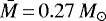 for both clouds. Since the IMF has a high-mass tail, clearly
  , but even assuming
  we conclude that 0.26≲ϵcore≲0.56.
Enoch et al. (2006) also fit their CMF with a log-normal distribution for M > 0.8 M⊙. They gave two values for Mpeak, namely 0.9 M⊙ and 0.3 M⊙, corresponding to Td = 10 K and 20 K, respectively, because they could not derive the dust temperature of each core, as we did with our data. If we want to compare their Mpeak with ours, we have to take into account both the different opacities (0.0074 cm2 g−1 following our opacity law instead of 0.0114 cm2g−1) and the different distance (300 pc here vs. 250 pc). Considering both differences, the two values for Mpeak become ~ 2 M⊙ and ~ 0.7 M⊙ for Td = 10 and 20 K, respectively. Our Mpeak is closer to the value corresponding to 20 K even if our range in Td (see Fig. 18) suggests that Td = 10 K should be more appropriate.
In Sect. 3.1, we derived a relation between distance and source coordinates. In Fig. 20, we show the resulting CMF for prestellar cores when each source is assigned a different distance. We note that physical radius increases with d while mass increases as d2, and therefore, in general, αBE ∝ d−1. As a consequence, objects that are closer will generally have lower αBE and objects that are further will have higher αBE. In any case, we find that changing the distance affects our prestellar core counts only minimally as the number of robust prestellar sources remains at 199 while the number of candidate bound cores increases by 1, from 100 to 101.
Including a varying distance, the log-normal fits do not change significantly: the peak for the robust prestellar cores is Mpeak = 0.816 ± 0.038 M⊙ while that for all the bound cores, that is both robust and candidate bound cores, is Mpeak = 0.464 ± 0.034 M⊙. The two sets of values (with fixed and varying distance) are equivalent within the uncertainties. On the contrary, the slope of the high-mass power law changes: for M > 1.03M⊙ there are 92 sources and the average of the slopes found with 4 and 23 bins becomes − 2.398 ± 0.026, different from the Salpeter value at 1.8σ. Even if Eq. (1) is only an approximation, it nevertheless highlights the importance of assuming a non-uniform distance for a complex like Perseus.
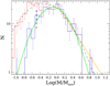 |
Fig. 19 Core mass function (dN/d logM) for the 199 robust prestellar cores (blue histogram), and for the 299 robust and candidateprestellar cores (red histogram) in Perseus. The two distributions overlap above M ~ 1.2. Histogramsuse a bin size of logM = 0.1. Green and dashed grey lines show a log normal fit, and the orange line shows a power-lawfit (see text for details). The dashed black line shows the completeness limit at ~ 0.32 M⊙. |
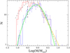 |
Fig. 20 Prestellar core mass function (dN/d logM) for sources in Perseus when each core is assigned a different distance based on Eq. (1). Lines as in Fig. 19. |
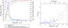 |
Fig. 21 Left panel: comparison of robust bound cores and starless cores. Histograms with the y-axis on the left show the distributions of all starless cores (blue) and all bound cores (green). The red and black lines (right y-axis) show cumulative surface density distributions for all bound cores and the off-filament bound cores, respectively. These distributions were derived by dividing the number of cores found at a certain N(H2) level by the total area in the image where the density is below that value. Right panel: prestellar core mass vs. background N(H2). Triangles are the mean mass averaged over bins of 1021 cm−2. The linear fit is shown as a red line. |
5.2 Link between filamentary structure and star formation
One of the key results from Herschel observations is the deep link between filamentary structures and the star formation in clouds. Numerous studies have shown that star formation preferentially occurs within filaments, with dense prestellar cores primarily in denser filaments (e.g. André et al. 2014, and references therein). This correlation has led to a possible paradigm, where filaments fragment into prestellar cores by gravitational instability (André et al. 2019).
We derived the number of robust prestellar cores inside a filament in two ways: in the most conservative approach, a core is considered internal to the filament if its distance from the spine is less than the width of the filament, or, more precisely, 1.29 × FWHM. In the relaxed approach, we simply require that the core be inside the filament border (refer to Sect. 3.2.3 and Fig. 11). The first, conservative sample consists of 167 bound cores (84% of the total) with a median mass of 1.0 M⊙. The second, relaxed sample contains an additional 23 (12%) bound cores, with a median mass of 0.96 M⊙. The remaining 9 (4%) prestellar cores have a median mass of 0.47 M⊙. Bound coresare therefore preferentially found within filaments, where the more massive cores are found.
For the unbound cores, the percentages for the three samples (conservative, relaxed, and out of filaments) are 47%, 14%, and 39%, respectively, with median masses of 0.10 M⊙, 0.15 M⊙, and 0.073 M⊙.
Figure 21 compares the background column density measured by getsources for the 519 starless cores (blue line) and 199 robust prestellar cores (green line; adding the 100 candidate prestellar cores shifts the distribution upwards but does not change the conclusions). The low number of cores at high density reflects to some extent the fact that regions with high N(H2) have an intrinsically smaller area than regions at low density. To check for this geometrical bias, we also plot in the same figure the cumulative distribution of bound cores normalised to area. The red curve shows the distribution for all 199 robust prestellar cores and the black curve shows the distribution for the 9 off-filament prestellar cores.
This cumulative distribution shows a few interesting features. First, about 90% of prestellar cores are found above ~ 2 × 1021 cm−2, in line with the value of ~2 mag found in Lupus (Benedettini et al. 2018). Higher values are instead found in Aquila (7 mag, Könyves et al. 2015) and in L1495 (6 mag, Marsh et al. 2016). Second, we find two separate regimes in the distribution: an almost linear regime up to ~ 5 × 1021 cm−2 below which ~60% of bound sources are found, followed by a flatter distribution.
The distribution of the off-filament prestellar cores shows a different trend (clearly, the on-filament distribution overlaps almost perfectly with the cumulative distribution for all bound cores). For the off-filament cores, all but one of the sources are found at N(H2) < 5.5 × 1021 cm−2.
One might speculate that off-filament sources are less massive than on-filament sources because the former are found at lower background column density than the latter. However, this is not the case because if we consider the median of the mass for sources that have N(H2) < 5.5 × 1021 cm−2, we find ~0.9 M⊙ for on-filament sources. For off-filament sources, the median of the mass is only 0.24 M⊙.
The right panel of Fig. 21 shows the mass of prestellar cores as a function of the background column density. We find a relatively flat mass distribution up to a threshold of 15 × 1021 cm−2. Above this threshold, sources are found only on-filament (more precisely 8 out of 9 off-filament bound cores are below 5.5 × 1021 cm−2) and their masses grow with the background column density with a slope 1.06 ± 0.23 M⊙ 10−21 cm2, if a linear trend is assumed (red line in figure).
The distributions shown in Fig. 21 raise the question of why we do not detect prestellar cores below 0.9 × 1021 cm−2. For example, the prestellar core with the smallest level of column density has a mass of 0.87 M⊙, which is 2.7 times above the completeness limit. The area of the map at column densities lower than this limit is 40% of the total map. If cores were distributed randomly, we would expect 90 prestellar cores of any mass to be found at low column density values14. The fact that we do not find bound cores at such low column densities implies that column densities N(H2)≳1021 cm−2 or AV≳1 are necessary for prestellar cores to form.
The possible existence of an AV threshold for star formation in Perseus was already investigated in the past with contrasting results. Hatchell et al. (2005) found no column density cutoff for dense cores based on C 18 O (1–0) observations, whereas Kirk et al. (2006) found that submillimetre clumps were detected only at AV > 5–7 mag. Sadavoy et al. (2010) found that 94% of SCUBA-identified sources were located at N(H2) > 3 × 1021 cm−2. Above the same level of column density, we find 63% of our sources.
In Fig. 22 we show the histogram of the minimum distance between cores. For robust bound cores, the distribution has a median value of 0.29 pc with a broad peak in the range 0.15–0.37 pc. However, for unbound cores the distribution has a median of 0.47 pc with a broad peak shifted to slightly larger separations than in the previous case, namely between 0.23 and 0.73 pc. For the tentative bound cores the median is 0.74 pc.
If cores were distributed uniformly across the observed region, one would expect a mean distance among bound cores of 0.69 pc, a factor 2.4 larger than the observed value of 0.29 pc. For starless cores, the mean distance is 0.65 pc, a factor 1.4 larger than 0.47 pc. This difference implies that prestellar cores cluster to some extent. This clustering is evident in Fig. 23, which shows the position of all the prestellar cores (red crosses) and of the unbound cores (green crosses). We find that sources do not appear uniformly distributed, but with few exceptions they are confined inside the regions defined in Fig. 9.
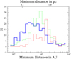 |
Fig. 22 Minimum distance between bound cores (blue), unbound cores (green), and tentative bound cores (red). |
Slope of the PDF and SFE for the subregions with known protostars.
5.3 Star-formation rate and efficiency, and core formation efficiency
The star formation rate (SFR) and star formation efficiency (SFE) are two fundamental properties derived from observationsthat any star-formation theory has to address, explain, and predict. The former is usually estimated as the total mass of young stellar objects (YSOs) divided by the mean duration of star formation (e.g. 2 Myr, Evans et al. 2009).
The total mass of YSOs is usually computed as the number N of YSOs multiplied by the representative value of 0.5 M⊙. It is clearly necessary to determine N as precisely as possible. Indeed, Herschel observations aimed to achieve better completeness for starless cores rather than YSOs, and so from our data alone we cannot derive a reliable SFR for Perseus.
The SFE is defined as the total mass of YSOs divided by the total mass Mcloud of the cloud, that is, the mass of protostars plus gas. For each subcloud, the SFE depends on how the border is defined. As we have already discussed in Sect. 3.2.2, defining such borders is not obvious. Sadavoy et al. (2014) computed dense cloud masses for the Perseus subclouds using a column density threshold of N(H2) = 1022 cm−2, chosen to select material primarily found in the high-column-density power-law tail. Here we follow another approach based on the local properties of each subcloud. Namely, we find for each subcloud the minimum background column density at the positions of the protostars in each region and compute Mcloud for N(H2) >min. In Table 9, we report for each zone the number of protostars, the minimum background column density where a protostar is found, the mass of the subcloud within this minimum value, the exponent s of the power-law fit to the associated PDF (see Sect. 3.2.4), and the respective SFE(%) = ∑ MYSO∕(∑ MYSO + Mcloud). The number of protostars associated to the whole Perseus cloud is 126 instead of 132 because five sources fall in the region observed with PACS only, and one source is in a region masked out for 250 μm extraction because of its close proximity to the border of the SPIRE map. In both cases the column density was not computed. L1451, B1E, and L1468 were not included because no protostars were found.
For the whole Perseus cloud, the minimum column density associated with a protostar is 0.64 × 1021 cm−2, below the limit of 1.6 × 1021 cm−2 that defines the last closed contour in the density column map. For this reason, the total mass of the cloud for N(H2) >min is likely underestimated. If we consider only protostars above the last closed column density contour, we find 113 protostars whose minimum N(H2) is 1.65 × 1021 cm−2. The total mass is now 6198 M⊙ and the SFE becomes 0.9%.
Sadavoy et al. (2014) found a linear correlation between SFE and slope s of the PDF, SFE ∝ 0.02s, and they discussed the implications of such correlation. These latter authors identified candidate Class 0 sources through their detectability at 70 μm, excluding objects that could be more evolved, namely Class I and Class II sources. As our column density map and slopes s are different from those derived by Sadavoy et al. (2014), as discussed in Sects. 3.2.2 and 3.2.4, one may wonder whether or not their result still holds with our data. This question cannot be properly addressed in this paper because in our work we used the criterion of 70 μm visibility to pick up potential protostars in our catalogue, without separating sources into Class 0, I, or II (see Sect. 4.1). Nonetheless, to give at least an indication of whether or not the Sadavoy et al. (2014) linear correlation is also present in our data, we made a linear fit using fifth and sixth columns of Table 9, finding SFE ∝ 0.013s; see Fig. 24. Therefore, even with the caveat on the used sample, we confirm the correlation between SFE and s.
As the Herschel-based catalogue is more complete in starless cores than in YSOs, it is more reliable to derive from our sample the core formation efficiency (CFE) than the SFE. Similarly to the latter, the former is computed as CFE(%) = ∑ Mpre∕(∑ Mpre + Mcloud) where we use only prestellar cores because unbound cores are less likely to form stars. For the CFE, we used the core masses computed during SED fitting instead of assuming a constant 0.5 M⊙ value as done for SFE. The results are reported in Table 10. Column N gives the number of prestellar cores per subcloud. In a few cases there is also an uncertainty for N, which we explain below. NII is the number of Class II objects given by Young et al. (2015). These latter authors also counted NII for the rest of the cloud (RC) defined as the whole of Perseus without IC348 and NGC 1333. In Table 10 we define RC as the whole of Perseus but without the four subregions for which the number of Class II objects was found. Column N(H2) has the same meaning as in Table 9: the minimum background column density at the position of the prestellar cores in each region. Mass M, CFE, and area are then computed for N(H2) >min. The ratio M/area gives the surface density reported in the Σ(gas) column. Finally, tpre is the estimated lifetime of the prestellar core phase, derived by scaling the number of bound cores to the number of Class II objects, and assuming a constant SFR: tpre = Npre∕NII × tII. As before, we fixed tII to the usually adopted value of 2 Myr for the duration of the Class II.
The uncertainty in tpre was derived based on αBE, the criterion used to define bound a core (see Sect. 4.3). We first derived the uncertainty ΔαBE from the uncertainties on mass and temperature for each source. Amoung the bound cores we then counted the number of sources with αBE + ΔαBE > 2: within the uncertainty, these sources could be unbound cores. Let us call this number N−. Similarly, unbound or candidate bound sources with a reliable SED and with αBE − ΔαBE ≤ 2 could be potential prestellar cores. We define N+ as the number of these sources. Table 10 provides the number of prestellar cores as  for the subclouds for which NII has been estimated. Here, tpre was not computed for the other subclouds for which an estimate of NII is not available. The uncertainty on N is assumed as max(N+, N−). This uncertainty is then propagated to tpre. The resulting lifetime for the whole Perseus cloud is tpre = 1.69 ± 0.52 Myr, which overlaps, within 1σ, with the value 1.2 ± 0.3 Myr found in Aquila by Könyves et al. (2015).
We see that for L1455 and B1, tpre is much higher than for the other regions. This could be explained if both clouds were very young, such that star formation started very recently. In this case, the number of Class II objects is less than expected assuming a constant SFR (for a similar case reported in Lupus I and Lupus IV, see Rygl et al. 2013). On the contrary, in NGC 1333 and IC348 we observe a deficit of prestellar cores compared to Class II objects. This can be interpreted as a decelerating SFR in these two regions, with IC348 having the shortest lifetime, in line with the known fact that this cloud is the oldest of the Perseus complex. We do not have the number of Class II stars for the other regions, but the relatively high tpre for RC might suggest that star formation also started recently in the other subclouds.
In Fig. 25 we show the CFE as a function of the PDF power-law exponent. Similarly to the case of SFE, for CFE we can also consider the threshold in column density of 1.6 × 1021 cm−2. In doing so, N decreases to 196 with a CFE of 4.5%, which is the value used in Fig. 25. The red line is a linear fit to all the data with a slope of 2.4. Here, HPZ6 appears to be an outlier; if its value is not used in the fit then the result is the black line, with a slope 1.22.
The mean value of all the subclouds excluding Perseus as a whole is 8.2 ± 4.8% or 7.2 ± 2.8% if we exclude the HPZ6 zone: the CFE of the whole cloud is within 1σ of these values. Another important timescale to compare with our estimate of the prestellar phase duration is the free-fall time, that is, the time required for a uniform sphere of density ρ and pressureless gas, i.e. gas at zero temperature, to collapse to infinite density (e.g. Krumholz 2015):
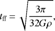 (10)
(10)
where G is the gravitational constant and ρ is the uniform density.
In Fig. 26 we show the distribution of tff for the 199 robust bound cores. The Gaussian fit to the distribution, plotted in red, shows a peak at 0.16 ± 0.01 Myr and σ = 0.06 ± 0.01 Myr, where we assigned an uncertainty of 0.01 Myr (half the size of the histogram bin) to both parameters. For a star of 0.25 M⊙, corresponding to the peak of the IMF, this implies a mean mass accretion rate of Ṁ ~ 1.6 × 10⁻⁶ M⊙ yr−1. Our peak of 0.16 Myr is close to the value of 0.10 Myr derived by Mercimek et al. (2017) using the sample of 69 cores defined by Sadavoy et al. (2010).
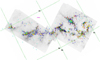 |
Fig. 23 Column density map overlaid with the positions of the 299 prestellar cores (yellow crosses and red crosses are robust and tentative cores, respectively), 220 unbound cores (blue hashes), and 132 protostars (cyan asterisks; we note that these sources were detected on the 70 μm map, which does not overlap completely with the SPIRE field of view, and so five cores are found outside the column density map). The map is rotated by 28°, with the top and bottom corners cut out. The magenta line in the centre shows the angular scale corresponding to 1 pc at 300 pc; J2000.0 coordinates grid is shown. |
 |
Fig. 24 Star formation efficiency as a function of the PDF slope for the different subclouds in Perseus, and for the whole cloud. The red point is an alternative SFE for Perseus (see text). The cyan line is a linear fit without taking into account uncertainties on the x-axis. |
CFE for all the subregions in Perseus with at least one bound starless core; where protostars are observed, the lifetime of the prestellar phase is also shown.
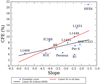 |
Fig. 25 Coreformation efficiency as a function of the power-law slope of the PDFs for the different subclouds in Perseus, and for the whole cloud. |
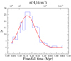 |
Fig. 26 Distribution of free-fall time for robust prestellar cores. Top-axis is the uniform density for spherical cores (3M∕4πR3). The red lineis a Gaussian fit. |
6 Conclusions
In this paper, we analyse photometric observations of the Perseus complex executed with PACS at 70 and 160 μm, and SPIRE at 250 μm, 350 μm, and 500 μm. We can summarise our main conclusions as follows.
- 1.
Using distances to protostars from Gaia DR2, we find a linear correlation between coordinates (α, δ) in the cloud and distance across the whole Perseus cloud. Although qualitatively already suspected, this correlation is the first estimate of such a trend. Distances estimated from our relation do not take into account the depth of the region at any point and are meant to give representative values; but they are not limited to a few lines of sight and are in very good agreement with other recent and more statistically robust estimates reported in the literature. We confirm that 300 pc is a good mean distance value for Perseus.
- 2.
We produce dust-temperature and column density maps. We find dust temperature to be in the range 10–28 K. Two main peaks in Td distribution are present at 16.4 and 17.1 K, corresponding to the average temperature of the diffuse medium in western and eastern halves of Perseus, respectively. A small bump is present at 19.2 K, which is associated with the inner part of NGC 1333 and IC348. The column density range is 2.5 × 10²⁰–1.4 × 1023 cm−2 with the smallest closed contour at 1.6 × 1021 cm−2. Td and N(H2) are found to be anticorrelated throughout the complex, with the exception of the inner parts of NGC 1333 and IC348, which are both warm and dense. We also show that a lack of data at λ < 160 μm causes Td to be underestimated by more than 10% for Td > 22 K.
- 3.
Extrapolating the column density and temperature maps to 70 μm shows that most of the cloud would appear as infrared dark clouds if observed with enough sensitivity. We also find excess emission at 70 μm above the extrapolated fluxes, which we attribute to very small dust grains.
- 4.
We find that the optical depth derived from our column density map, and extrapolated at 850 μm, agrees with that measured with Planck for τP < 3 × 10⁻⁴, where τP is the optical depth measured by Planck. At higher τP, the optical depth found with Herschel is higher than that found with Planck data. This could be due to a change in the dust opacity. On the contrary, our column density map disagrees with the column density maps derived from near-infrared extinction maps if masses within the same AV contour are compared; better agreement is found when masses are derived from the same areas in the two maps. In any case, the comparison is not easy because of the varying dust opacity, or because in star-forming regions R ≡ AV∕E(B − V) > 3.1 and in Perseus it is also variable throughout the complex.
- 5.
We find a typical filament width of 0.08 pc for an assumed distance of 300 pc, confirming the general result of previous HGBS studies that a characteristic filament width of 0.1 pc exists in star-forming regions.
- 6.
On average, star-forming filaments in Perseus have mean line masses significantly below the critical value of 16 M⊙ pc−1, above which an isothermal filament at 10 K and infinite radius becomes unstable to radial collapse. However, we suggest that with a proper internal volume density, a filament with a line mass as low as 8 M⊙ pc−1, which is half the critical line mass, can fragment.
We extracted compact cores from the intensity maps and used SED fitting to determine their masses and temperatures. Our findings are as follows.
- 7.
We find 199 starless cores have greater masses than their corresponding Bonnor-Ebert masses, above which an isothermal sphere of gas cannot provide sufficient support against gravity. These cores are therefore thoughtto be collapsing, or to be close to collapse, and to be forming stars. We define these sources as robust bound or prestellar cores. Another 100 cores may also be collapsing and we define these as candidate prestellar cores. On the other hand, 220 sources have masses below their corresponding Bonnor-Ebert threshold and so they are not thought to be dominated by gravity. We name these objects unbound cores. We also declare 132 cores as protostars, because they show, through emission at 70 μm, that an internal source of energy should already be present. Finally, the remaining 165 sources cannot be satisfactorily fit with a modified blackbody because their SEDs are too uncertain.
- 8.
On the M − R plane, starless cores do not trace a clear path but show a large scatter with a faint hint of a correlation between M and R. Ignoring the scatter and fitting a power law anyway, we find M ∝ R1.28 for unbound sources. A similar relation is found for candidate prestellar cores: M ∝ R1.32. However, for bound sources, we find M ∝ R0.25, a relation that is shallower than expected for Bonnor-Ebert spheres (M ∝ R). We suggest that our slope of 0.25 likely reflects the lack of a correlation for the prestellar cores as a whole, which is probablya hint that these sources are indeed collapsing. From M and R, we derive a mean column density for sources that appears anticorrelated with temperature, with different exponents for bound and unbound sources.
- 9.
We find that M and T are also anticorrelated. We show that, for a given T, the smallest detectable mass of an unbound core is given by a combination of the Herschel instruments sensitivity, which gives a relation M ∝ T−4, scaled by an empirical factor that is likely due to the presence of the bright diffuse medium in which cores are embedded. However, for bound cores, the relation is much steeper M ∝ T−12, which is probably a consequence of the fact that more massive and colder bound cores are found in brighter regions of the clouds.
- 10.
The prestellar CMF can be modelled with a log-normal curve with a peak at M ~ 0.82 M⊙, which is above the completeness limit in mass estimated at 0.32 M⊙. Assuming a one-to-one mapping of the CMF over the IMF, this peak implies a core mass efficiency of 0.30. The high-mass tail of the CMF can be modelled with a power law with a slope of − 2.321 ± 0.035, which is in agreement, at 1σ, with the Salpeter IMF value of –2.35. The two distributions, log-normal and power law, were modelled separately because the number of bound cores is not large enough to make a combined fit; for the same reason, we cannot decipher whether or not one distribution alone can fit the whole dataset.
- 11.
More than 84% of robust bound cores are found within filaments versus 47% for unbound cores. On-filament bound sources are on average more massive than the off-filament ones. No bound cores are found below 0.9 × 1020 cm−2. Should sources be distributed uniformly on the map, 90 prestellar cores of any mass should have been found at column densities lower than that value. We propose that a limit of ~1 × 1021 cm−2 in column density is required to form bound cores.
- 12.
We find a correlation between SFE and the slope of the column density PDF for different Perseus subclouds. The correlation has a slope of 1.3%. We also find a correlation between SFE and CFE, with a slope of between 1.2 and 2.4%, depending on wether we use all the subclouds or exclude one extreme value from the sample.
- 13.
Assuming a constant SFR we derive a lifetime for the prestellar phase tpre of 1.69 Myr for Perseus but with significant scatter for the individual subclouds.
- 14.
We find a typical free fall time of 0.16 Myr, which implies a mean mass accretion rate of Ṁ ~ 1.6 × 10⁻⁶ M⊙ yr−1 to form a star of 0.25 M⊙, which is at the peak of the IMF.
The catalogue of all 816 detected sources is presented in the Appendix A where we give an example of a protostar, a prestellar core, and an unbound core. The full catalogue can be found at the CDS.
We also list in Appendix E sources that were excluded from our analysis, such as galaxies for example. This catalogue is not part of the HGBS official products, and is presented here in its entirety.
Acknowledgements
We thank the anonymous referee for the valuable comments that improved the readability of the paper. S.B. and N.S. ackowledge support by the french ANR and the german DFG through the project “GENESIS” (ANR-16-CE92-0035-01/DFG1591/2-1). P.P. and D.A. acknowledge support by FCT/MCTES through national funds (PIDDAC) by this grant UID/FIS/04434/2019. P.P. also acknowledge the support from the fellowship SFRH/BPD/110176/2015 funded by FCT (Portugal) and POPH/FSE (EC). PACS has been developed by a consortium of institutes led by MPE (Germany) and including UVIE (Austria); KU Leuven, CSL, IMEC (Belgium); CEA, LAM (France); MPIA (Germany); INAF-IFSI/OAA/OAP/OAT, LENS, SISSA (Italy); IAC (Spain). This development has been supported by the funding agencies BMVIT (Austria), ESA-PRODEX (Belgium), CEA/CNES (France), DLR (Germany), ASI/INAF (Italy), and CICYT/MCYT (Spain). SPIRE has been developed by a consortium of institutes led by Cardiff University (UK) and including Univ. Lethbridge (Canada); NAOC (China); CEA, LAM (France); IFSI, Univ. Padua (Italy); IAC (Spain); Stockholm Observatory (Sweden); Imperial College London, RAL, UCL-MSSL, UKATC, Univ. Sussex (UK); and Caltech, JPL, NHSC, Univ. Colorado (USA). This development has been supported by national funding agencies: CSA (Canada); NAOC (China); CEA, CNES, CNRS (France); ASI (Italy); MCINN (Spain); SNSB (Sweden); STFC (UK); and NASA (USA). HIPE are joint developments by the Herschel Science Ground Segment Consortium, consisting of ESA, the NASA Herschel Science Center, and the HIFI, PACS and SPIRE consortia. Part of this workhas received support from the European Research Council (ERC Advanced Grant Agreement no. 291294 – ORISTARS) and from the French national programs of CNRS/INSU on stellar and ISM physics (PNPS and PCMI). This research has made use of: the SIMBAD database, operated at CDS, Strasbourg, France; the NASA/IPAC Extragalactic Database (NED) and Infrared Science Archive which are operated by the Jet Propulsion Laboratory, California Institute of Technology, under contract with the National Aeronautics and Space Administration; data from the ESA mission Gaia (https://www.cosmos.esa.int/gaia), processed by the Gaia Data Processing and Analysis Consortium (DPAC, https://www.cosmos.esa.int/web/gaia/dpac/consortium). Funding for the DPAC has been provided by national institutions, in particular the institutions participating in the Gaia Multilateral Agreement. Figures showing the column density and temperature maps were done with DS9 (Joye & Mandel 2003).
Appendix A The catalogue
The CDS material provides data for all 816 candidate cores in the form of an atlas, one page per object. Figure A.1shows an example for a prestellar core (#49) and Fig. A.2 shows an example for a protostellar core (#55). For each core we provide the following:
-
A figure showing a 2′ × 2′ cutout around each source at 70 μm (top left), 160 μm (top middle), 250 μm (top right), 350 μm (bottom left), 500 μm (bottommiddle), and from the high-resolution column density map (bottom right). If the source is detected by getsources, a green ellipse shows the source size from the extraction. We note that some sources were not observed at all wavelengths, because PACS and SPIRE have slightly different fields of view.
-
Below the six cutouts, the figure on the left shows the observed SED (blue points) and its best-fit modified black body function (cyan curve). On the right we give the best-fit value for dust temperature (T) and mass (M) from the SED fit. Then, the source radius (R), that is the geometrical mean of major and minor FWHMs both measured from the high-resolution column density map, is given in arcseconds, before and after the deconvolution with the instrumental FWHM (18′′); the deconvolved radius is given also in parsecs in the third row. If a source is unresolved, we use a source size of <6′′.1 (or one-third of the beam). In this case the physical radius in parsecs is computed assuming R = 6′′.1.
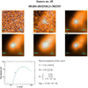 |
Fig. A.1 An example of the atlas of the Perseus cores showing the prestellar core #49. The original size of the page is A4, here thepage has been shrunk to one third. |
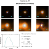 |
Fig. A.2 An example of the atlas of the Perseus cores showing the protostar core #55. Also in this case the page has been shrunk. |
Protostars were detected using the 70 μm intensity map only. As a residual misalignment may remain among the maps (see Sect. 2), the 70 μm coordinates of the centre may appear offset in the SPIRE intensity maps. The misalignment is smaller than the instrument spatial resolution, but before running getsources all the maps are reprojected onto a grid with pixel size 3′′, and so the displacement, if present, appears enhanced. Adopting the coordinates derived during the starless core detection the protostar would appear well centred at the SPIRE wavelengths but offset in the PACS bands. To show this effect, we use Fig. A.3 where the background image in both panels is the 250 μm cutout. In the upper panel, we show the ellipse and centre from the protostar catalogue (obtained from the PACS extraction), whereas in the bottom panel, we show the ellipse and centre from the starless core catalogue (obtained from the SPIRE extraction). Clearly, at 250 μm the source is better centred in the SPIRE extraction. Therefore, for protostars, data in the PACS bands were taken from the prostostars catalogue, while data in the SPIRE bands were taken from the starless catalogue.
A similar problem occurs at 160 μm for starless cores. In this case, the detection is done in the SPIRE maps, in the high-resolution column density map and in the 160 μm temperature-corrected map, but not in the 160 μm intensity map that is used for photometry extraction at the position found in the other maps. This strategy could be what causes many of the sources to have only an upper limit at 160 μm and in somecases the upper limit poses a problem when fitting the SED. In Fig. A.4 we show such an example. The top-left panel shows the cutout in the PACS red band where getsources could not detect any source. However, even by eye it is possible to see that some emission is present at the position of the source that was not recognised as a real object. The bottom-left panel shows the corresponding SED with the 3σ upper limit estimated with getsources.
We testour strategy by performing an alternative extraction using all five Herschel intensity maps simultaneously. The benefit of this approach is that the direct detection at 160 μm may help toextract photometry at this wavelength for weak sources. This alternative catalogue was used only to see if we could assign a measurement to sources with a stringent upper limit at 160 μm, like the one in Fig. A.4, with the conventional strategy. We found measurements for 12 sources using the alternative extraction. The top-right panel of Fig. A.4 shows that now the starless core is detected also at 160 μm. In the bottom-right panel we show how the SED fitting benefits from this measurement.
The new 160 μm measurement has a large impact on the source physical parameters, with the temperature increasing from 10.42 K to 16.14 K and the mass decreasing from 0.627 M⊙ to 0.073 M⊙. As there are 22 sources in the final catalogue with masses 0.6 ≤ M∕M⊙ < 0.7, two of which have no reliable SED fit, it is clear that removing even one single source may have some impact on the CMF.
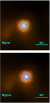 |
Fig. A.3 Coordinates of source #55 at 250 μm as derived in the protostars (top) and starless cores (bottom) catalogues, respectively. |
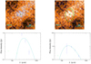 |
Fig. A.4 Effects on the SED when using an alternative extraction strategy (see text). Top panels: undetected and detected source at 160 μm. Bottom panels: SEDs with an upper limit and measure at 160 μm. |
Another approach with which we tried to solve the problem of the upper limits at 160 μm was to exclude this value during the fitting procedure. When getsources cannot detect a source found in other images at a certain wavelength, it sets the so-called monochromatic significance to the special value 9.999E-31. When we found it evident that the upper limit at 160 μm was influencing the SED fit much more than the SPIRE measures, we changed this value to 9.999E-30. In this case the fitting code uses the “extracted” 160 μm intensity as if it is reliable, but assigns it a very low weight such that this band is not used to constrain the fit. This strategy was already used in a study of Lupus (Benedettini et al. 2018). We show the result of this procedure when applied to source #58 in Fig. A.5.
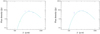 |
Fig. A.5 Effects on the SED when the measurement at 160 μm is used instead of the upper limit for undetected sources (see text). Left panel: best-fit with upper limit; right panel: best-fit witha measure. |
In the left panel we show the SED and best-fit modified blackbody function of this core as derived by getsources: it is clear that the upper limit in the red band forces the best-fit to have a low temperature. The best-fit has T = 7.74 ± 0.02 K and M = 8.59 ± 0.45 M⊙, a large mass indeed. On the other hand, using the total flux density at 160 μm that getsources measured at the position of the core in the other bands gives the SED shown in the right panel of Fig. A.5. The 160 μm value has a very low weight and so the best-fit is now determined by the SPIRE intensities only and the parameters become 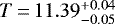 K and M = 0.330 ± 0.014 M⊙, much more reasonable values for Perseus.
We usedthis method to “correct” the SED of 139 unbound cores with reliable SED fitting, 51 prestellar, and 5 likely bound sources. A much more simple approach would be to completely ignore the upper limit, but we find that in some cases the best-fit model agrees well with the 160 μm measurement even if it is not relevant during the fitting procedure. This means that in this case getsources is able to produce a reasonable measurement even without directly detecting the source. The reader will recognise the ‘corrected’ sources because in these cases the ellipse showing the size of the core (see Figs. A.1 and A.2) is drawn in red instead of green.
In the following section on the completeness limit, we provide a precise assessment of the validity of these two approaches to the problem of the 160 μm upper limit, because in that case we deal with simulated sources for which we know the true values of the physical parameters.
The master catalogue listing the observed properties of all the cores is available at the CDS. A template is provided in Table A.1 to illustrate its form and content which follows Könyves et al. (2015). There are cases in which two Spitzer sources can be associated with one Herschel protostar. In this case we chose the Spitzer source detected at 70 μm, exploiting the fact that in no case both sourceshad detections at 70 μm. If none wasrevealed in this band, we associated the source with the higher 24 μm detection.
The derived properties (physical radius, mass, SED dust temperature, peak column density at the resolution of the 500 μm data, average column density, peak volume density, and average density) are given in another table also available at the CDS. Table A.2 gives an example. We note that for protostars the derived properties refer to the external envelope. A more detailed SED fitting will be the object of a forthcoming paper.
Catalogue of dense cores identified in the HGBS maps of Perseus molecular complex.
Catalogue of dense cores identified in the HGBS maps of the Perseus molecular complex.
Catalogue of dense cores identified in the HGBS maps of the Perseus molecular complex.
In a third table we provide additional data for each source; see the sample in Table A.3. Columns (2) and (3) give the source luminosity in two ways. First, for a modified blackbody the bolometric luminosity Lbol, can be computed analytically as shown by Elia & Pezzuto (2016). For β = 2,
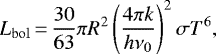
where σ is the Stefan-Boltzmann constant, k and h are the Boltzmann and Planck constants, T is the dust temperature, and ν0 = c∕λ0 where λ0 is the wavelength above which the model becomes optically thin. For a given dust opacity parametrised with a power law of parameters (λref, κref, β), λ0 is (Pezzuto et al. 2012)
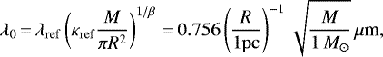 (A.1)
(A.1)
with R and M being the radius and mass of the (spherical) source.
The bolometric luminosity then becomes
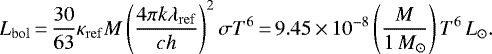 (A.2)
(A.2)
Equation (A.2) implies an integration of the whole SED, even at λ < λ0 where the modified blackbody becomes optically thick. However, Elia & Pezzuto (2016) showed that the SED does not necessarily have to be optically thin at all wavelengths for Eq. (A.2) to be valid, and that it is enough that optical depth is less than 1 for λ = λ⋆ where λ⋆ is defined by the condition
 (A.3)
(A.3)
with x⋆ = hc∕kλ⋆T. For β = 2 the integral becomes negligible (< 0.01) at x⋆ = 15. This implies that the dusty envelope should already be optically thin at λ⋆ = 960∕T μm.
Columns (4) and (5) in Table A.3 report λ0 and λ⋆ for each model, while Col. (3) gives the luminosity obtained by numerical integration of the SED at Herschel wavelengths. For the first source in the table, the model becomes optically thin at 82 μm, while λ⋆ is 131 μm. In other words, the analytical formula for Lbol is efficient as long as the model is optically thin at 131 μm which is correct given that λ0 = 82 μm.
The second source is a protostar. In this case Lbol cannot be computed with Eq. (A.2), meaning that Col. (2) is not correct and one can use Col. (3) as a measure of the FIR luminosity. The third source does not have a reliable SED fit, meaning that M and T were not derived from the SED. In this case, Cols. (2), (4), and (5) report a zero while Col. (3) gives a more precise FIR luminosity.
Column (6) reports the kind of core: “0” is unbound, “1” is prestellar, “2” is protostellar, and “3” is candidate. Column (7) gives the reliability of the SED fitting: “1” means that the SED could be fit with a modified blackbody, “0” otherwise. Column (8) gives the region to which each source is associated, the numerical correspondence is given in the caption. These last three columns allow us to make selections on the sample of cores easily: for instance, to select prestellar cores in IC348 one can look for sources with (1,1,9) in these columns.
Appendix B Simulation of prestellar cores
A total of 432 simulated prestellar cores with Bonnor-Ebert density profile and mass between 0.05 M⊙ and 0.96 M⊙ were injected into the source-free intensity maps to verify the correctness of our extraction procedure and to derive the mass completeness limit. The simulations were performed as in previous HGBS studies (Könyves et al. 2015; Marsh et al. 2016; Benedettini et al. 2018). The extraction of the simulated sources was performed nominally and the post-selection checks for cores described in Sect. 4.1 were executed. This catalogue was then cross-checked against the truth table of the synthetic cores and 315 sources out of the 432 were recovered.
B.1 Restoring the 160 μm intensity
As discussed in the previous section, we found some problems when dealing with the 160 μm upper limit often found in the standard extraction. To prevent the upper limit from forcing the SED fitting to overly low temperatures, we adopted two different strategies previously described and here we discuss their validity.
First, we carried out an alternative extraction using all five of the Herschel bands simultaneously. Compared to the nominal extraction, two sources with only upper limits at 160 μm ended up with intensity measurements in the alternative extraction. For one source, the mass derived from the SED fitting using the upper limit at 160 μm is 1.46 timesthe true mass. Using the measurement from the alternative catalogue, the derived mass is 1.36 times the true mass, which is slightly better. For the second source, using the upper limit causes the derived mass to be overestimated by more than a factor of three. Using the measured flux density in the alternative catalogue, the ratio is 0.75, which means that the mass is only underestimated by 25%, which is a better result in any case.
The second approach was to pretend that the upper limit in the nominal extraction is indeed a real measurement but with a negligible weight during the SED fitting so that it does not force the fitting. For 96 sources out of 147 simulated cores with an upper limit, nothing changed because the best-fit model fullfilled the upper limit, or because the SED could not be fit anyway. For the remaining 51 sources, the mean ratio between the SED-fitting derived mass and true mass is 1.5 ± 1.1 when using the upper limit, and 0.92 ± 0.78 when the 160 μm intensity is weighted down in the SED fit. A comparison between the two means show that the upper limit causes, on average, an overestimation of the mass by 50% while weighing down the 160 μm intensity ensures an agreement with the input mass within 8% on average. We conclude that the SED fitting improves in both approaches, even if in the second approach the large standard deviation of the means shows that the results are valid for the whole sample and not applicable to single sources.
B.2 Completeness limit in mass
In Fig. B.1 we show the fraction of detected sources with respect to the number of simulated sources as a function of the true core mass. To improve the statistics we summed the number of detected sources in three adjacent bins with similar masses, while the mass of each bin was the average of the three masses. The last two points are the sum/average of four bins.
The horizontal dashed line shows the 90% level of completeness while the vertical line corresponds to a mass of 0.323 M⊙, found by linear interpolation of the two bins at 0.290 M⊙ and 0.420 M⊙. The trend at high-mass in Fig. B.1 is also interesting, where the number of detected sources decreases. As shown by Könyves et al. (2015), the likelihood of detecting a sources does not only depend on its intensity, but also on the contrast, i.e. how wellthe source stands out above the emission of the diffuse medium. In general, high-mass cores are found in high-column-density regions which are very bright. To estimate the contrast we used the signal-to-noise ratio (S/N) expressed asthe peak intensity of the simulated sources over the standard deviation of the local background, both in MJy sr−1. This ratio, for the fiducial wavelength of 250 μm, is shown in Fig. B.2: blue and red triangles refer to detected/undetected sources, respectively. We can see that for S∕N ≥ 3 we detect ~98% of the sources independent on their mass. The percentage is as low as 31% for S∕N ≤ 1. At high mass we explored low levels of S/N that resulted in a small fraction of detected sources. This figure shows that high-mass cores are not necessarily found easier than low-mass cores. The interested reader is invited to read the in-depth discussion on this topic in Könyves et al. (2015).
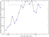 |
Fig. B.1 Number of detected sources over number of simulated sources vs. true core mass. The completeness limit is defined as the mass at which completeness is 90%: in our case this happens at 0.323 M⊙, the limit shown as intersection between the two dashed lines. The decrease in the number of detected sources at high mass is discussed in the text (see also next figure). |
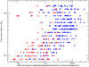 |
Fig. B.2 Contrast level (see text) for detected sources (blue triangles) and undetected sources (red triangles). |
Appendix C Definition of Perseus subregion borders through 13CO observations
The Perseus molecular complex is known to host different regions with distances varying between ≳200 pc and ≲350 pc. From our intensity maps, because the dust emission is optically thin, it is not possible to estimate which regions are closer or further. Also, their borders are arbitrarily defined.
To obtain some insight into these problems, especially for tracing the borders, we combined our column density map (Sect. 3.2) with the 13CO map of Perseus (COMPLETE team 2012). In particular, we started from the N(H2) contour at 3 × 1021 cm−2 and modified it in order to maximise one single velocity component in each region wherever possible. The result of this exerciseis visualised in Figs. C.1–C.2, where we show how the borders have been defined to accommodate the observed velocity components, and in Fig. C.3 which shows the 13 CO spectra within these borders. The regions are shown over the column density map in Fig. 9.
From these figures it is clear that only in a few cases is a region associated to one single 13 CO component; in general, two or even three components are present, often in the form of broad bump. The most complex case is NGC 1333 which appears bright from 6 to 10 km s−1. It is not possible to assess whether these different velocity components are associated to different distances or simply reflect the presence of complex motions of gas at the same distance.
Border coordinates are reported here in DS9 format.
# Region file format: DS9 version 4.1
global color=green dashlist=8 3 width=1 font=
"helvetica 10 normal roman" select=1 highlite=1 dash=0
fixed=0 edit=1 move=1 delete=1 include=1 source=1
image
# text(1487.4314,333.61838) color=blue
font="helvetica 10 bold roman" text={L1451}
polygon(1333.8089,437.23983,1440.7546,458.68454,
1470.8901,400.07136,1379.8181,321.59092,1318.014,
336.61325) # color=blue width=2
# text(1502.1189,499.27846) color=blue
font="helvetica 10 bold roman" text={L1448}
polygon(1356.7824,546.66324,1434.3763,539.49322,
1439.1677,463.43743,1310.8333,436.43609,1308.4301,
509.10723) # color=blue width=2
# text(1190.5906,242.44105) color=blue
font="helvetica 10 bold roman" text={L1455}
polygon(1157.7149,533.49812,1193.5852,541.55673,
1201.6303,532.283,1215.238,531.67128,1246.7729,
549.00541,1283.1111,422.1613,1327.4841,411.09164,
1304.5877,251.04107,1145.3085,315.92795,1158.7509,
368.22467,1165.0377,472.01562) # color=blue width=2
# text(1126.212,879.76219) color=blue
font="helvetica 10 bold roman" text={NGC1333}
polygon(1071.1585,853.15932,1132.7315,852.35554,
1230.2714,722.39349,1259.8445,725.13296,1277.862,
676.20236,1230.1883,669.20757,1240.7268,553.33499,
1203.1152,535.40696,1193.8331,545.29856,1168.4754,
541.57477) # color=blue width=2
# text(984.80575,409.03949) color=blue
font="helvetica 10 bold roman" text={Per6}
polygon(1036.4774,468.77807,1159.281,466.4625,
1156.1584,374.55727,1035.721,398.26535,1015.8924,
441.03821) # color=blue width=2
# text(925.20483,769.29545) color=blue
font="helvetica 10 bold roman" text={B1}
polygon(1044.0405,774.40647,1086.8576,705.50003,
1124.9583,562.11768,1054.5893,474.75889,1032.5161,
469.56833,980.24576,429.13633,935.86235,461.59737,
908.00317,506.37669,840.6034,618.84583,839.77572,
690.94226) # color=blue width=2
# text(805.68456,485.18367) color=blue
font="helvetica 10 bold roman" text={B1E}
polygon(746.29823,669.50423,771.72844,651.05987,
808.98863,653.10202,840.60823,610.13084,877.69561,
550.77242,804.47781,506.58305,696.42301,591.8366,
709.0804,630.66426,736.00938,648.1077) # color=blue
width=2
# text(489.66258,695.47969) color=blue
font="helvetica 10 bold roman" text={L1468}
polygon(627.59045,765.79554,668.84339,729.81106,
737.21644,796.78156,758.23062,698.28841,684.74148,
712.86762,652.8725,643.16733,617.50019,632.44604,
531.17747,534.78311,482.46366,598.33846,550.86898,
686.697,536.24192,701.54936) # color=blue width=2
# text(422.30564,920.67911) color=blue
font="helvetica 10 bold roman" text={IC348}
polygon(239.96759,887.13841,252.9806,907.15254,
274.84348,925.7651,306.5413,955.20126,347.81727,
930.38764,380.28695,871.58782,467.83656,900.06909,
495.59982,884.78731,515.42993,905.80607,613.92733,
913.78255,636.89789,891.3492,613.76131,834.94829,
610.25222,781.98471,564.80593,745.37937,363.56661,
721.83811,327.29322,675.35843,266.47791,722.34789,
279.74514,781.64591,345.61729,808.68617,250.32306,
816.90053,300.46231,842.71522,317.67854,875.81041,
263.01753,887.93356,251.07107,885.34014) # color=blue
width=2
# text(231.55717,1080.3695) color=blue
font="helvetica 10 bold roman" text={B5}
polygon(131.84123,1149.1204,204.32139,1146.0994,
199.21689,1063.8127,368.68022,1016.0499,227.01718,
963.66495,101.94755,1020.7039,123.39263,1035.5521,
78.991784,1084.8691,115.25351,1089.8388) # color=blue
width=2
# text(1458.7042,766.89968) color=blue
font="helvetica 10 bold roman" text={HPZ1}
polygon(1259.8775,743.24297,1331.4864,780.605,1438.2509,
703.67412,1504.4839,566.14416,1288.6928,658.07238)
# color=blue width=2
# text(944.78788,261.33954) color=blue
font="helvetica 10 bold roman" text={HPZ2}
polygon(979.47848,380.01503,1009.5859,377.65325,
1091.2147,328.57301,1091.2463,264.39894,1030.2487,
250.1076,979.51784,301.58003) # color=blue width=2
polygon(269.65329,875.23531,314.0925,875.68734,
296.44116,841.19846,249.80269,820.81436) # color=blue
width=2
# text(811.58094,726.68431) color=blue
font="helvetica 10 bold roman" text={HPZ3}
polygon(801.04278,684.50226,828.78401,698.12952,
828.70223,652.90765,774.89423,659.87374,777.25972,
684.49736) # color=blue width=2
# text(638.77426,606.92082) color=blue
font="helvetica 10 bold roman" text={HPZ4}
polygon(688.10315,706.15275,740.73908,694.85417,
736.00504,655.23816,697.21552,630.51863,684.53517,
623.01812,653.71632,634.77201) # color=blue width=2
# text(685.39798,440.72586) color=blue
font="helvetica 10 bold roman" text={HPZ5}
polygon(587.24505,484.82277,660.47976,537.87714,
709.20818,522.27317,700.28996,493.47845,604.90108,
444.89766) # color=blue width=2
# text(197.62231,846.05505) color=blue
font="helvetica 10 bold roman" text={HPZ6}
polygon(269.65329,875.23531,314.0925,875.68734,
296.44116,841.19846,249.80269,820.81436) # color=blue
width=2
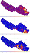 |
Fig. C.1 Maps of 13CO in three velocity channels: 1.1 Km s−1 (top), 4.35 Km s−1 (centre), 6.0 Km s−1 (bottom); colour bars are uncorrected antenna temperature in K. Green labels mark the position of Gaia sources (see Table 2); h labels show the position of Hirota et al. (2008) and Hirota et al. (2011) sources (SVS13 is in the cloud of sources 6-10). The magenta lines at the centre of each map show the angular scale corresponding to 1 pc at 300 pc; J2000.0 coordinates grid is shown. |
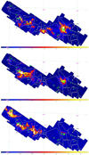 |
Fig. C.2 Maps of 13CO in three velocity channels: 7.9 Km s−1 (top), 8.8 Km s−1 (centre), 10.0 Km s−1 (bottom). In the latter panel, north of B5 and slightly covered by label 28, the bubble CPS12 (Arce et al. 2011) is evident. The magenta lines at the centre of each map show the angular scale corresponding to 1 pc at 300 pc; J2000.0 coordinates grid is shown. Labels as in Fig. C.1. |
 |
Fig. C.3 13CO spectra for all the subregions we defined in Perseus. Whenever possible we made a Gaussian fit to one or two profiles; forthe broad bumps we simply derived the position of the maximum and assigned it an uncertainty of 0.066 km s−1, which is equal to the step in the velocity grid. |
Appendix D Herschel intensity maps
In this Appendix we show the PACS intensity maps at 70 μm and 160 μm in Fig. D.1; SPIRE intensity map at 250 μm and the high-resolution column density map with a resolution of 18′′. 2 in Fig. D.2 (the column density map shown in Fig. 4 is at 36′′. 1); and SPIRE intensity maps at 350 μm and 500 μm in Fig. D.3. To help to localise the region of Perseus in other surveys, we provide a grid of coordinates in different systems: FK5 (equatorial) for 70 μm and 250 μm, Galactic for 160 μm, 350 μm and for the high-resolution column density map, ecliptic for 500 μm.
Maps centres, as given in FITS header and converted to the specific coordinate system are: (3h 36m43s,+31°35′27′′), or (54. °1775,+31. °5908) for blue band; (159.5082,–19.3010) for red band; (3h 35m06s,+31°31′20′′), or (53. °7732,+31. °5221) for PSW band; (159.3639,–19.4821) for the column density map; (159.4321,–19.5946) for PMW band; (59. °3449,+11. °7751) for PLW band.
From Figs. D.1–D.3 it is evident that the diffuse emission intensity increases at longer wavelengths, being marginally visible at λ = 70 μm.
Zero-levels of the diffuse emission for each map.
The zero-level intensities for the diffuse emission were found through comparison with the predicted Planck+IRAS emission (Bernard et al. 2010) for the same region. For each map and wavelength, the zero-level intensity was found separately for west and east Perseus and the offset added to the map. Finally, the two maps were combined with a simple pixel-by-pixel mean (the two maps were created on the same spatial grid). The offsets are reported in Table D.1.
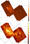 |
Fig. D.1 Combined maps of Perseus at 70 μm (top, grid of equatorial J2000.0 coordinates, HPBW 8′′.4) and 160 μm (bottom, grid of Galactic coordinates, HPBW 13′′.5). Colour bars in MJy sr−1. |
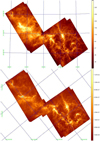 |
Fig. D.2 SPIRE intensity map of Perseus at 250 μm (top, grid of equatorial J2000.0 coordinates) and the high-resolution column density map (bottom, grid of Galactic coordinates). For both maps the HPBW is 18′′. 2. Colour bars are in MJy sr−1 (top) and cm−2 (bottom). |
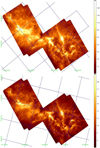 |
Fig. D.3 SPIRE intensity maps of Perseus at 350 μm (top, grid of Galactic coordinates, HPBW 24′′.9) and 500 μm (bottom, grid of ecliptic coordinates, HPBW 36′′.1). Colourbars in MJy sr−1. |
Appendix E Additional catalogue of sources
Here we report basic data for sources eliminated from the main catalogue; as these data are not part of the official HGBS delivered products they are reported here. The columns in the following tables are a subset of the columns in Table A.1, and the numbering is kept the same as for that table: e.g. the contents of Col. (12) in Table E.1 is the same as Col. (12) in Table A.1. The only difference is units in Col. (55): 1021 cm−2 in Table A.1 and 1020 cm−2 here.
The other difference is Col. (2) in this table: here an identifier is given that explains why a source was removed (acronyms ass in Simbad database): G – galaxy; W – counterpart in WISE catalogue; 2 – counterpart in 2MASS; HH – Herbig-Haro object; M – star from catalogue MBO; HL – candidate YSO from [HL2013]; DS – source in [DS95]; LRL – source in “Cl* IC 348 LRL”; PSZ – source in [PSZ2003]; NTC – source in “Cl* IC 348 NTC”; U – W UMa star; δ – δ Scuti star.
In particular, “W” and “2” means that an infrared sources was found in WISE or 2MASS catalogues within 6′′ of an Herschel source not detected at 70 μm nor in the millimetre band. No attempt was made to distinguish between physical and projected associations.
Catalogue of additional sources excluded from the main catalogue.
Same as Table E.1 for 250 μm and 350 μm.
Same as Table E.1 for 500 μm and high-resolution column density map.
References
- Alves, J., Lombardi, M., & Lada, C. J. 2007, A&A, 462, L17 [NASA ADS] [CrossRef] [EDP Sciences] [Google Scholar]
- Alves de Oliveira, C., Moraux, E., Bouvier, J., et al. 2013, A&A, 549, A123 [NASA ADS] [CrossRef] [EDP Sciences] [Google Scholar]
- Alves, J., Lombardi, M., & Lada, C. J. 2017, A&A, 606, L2 [NASA ADS] [CrossRef] [EDP Sciences] [Google Scholar]
- Andrae, R. 2010, ArXiv e-prints [arXiv:1009.2755] [Google Scholar]
- Andrae, R., Schulze-Hartung, T., & Melchior, P. 2010, ArXiv e-prints [arXiv:1012.3754] [Google Scholar]
- André, P., Men’shchikov, A., Bontemps, S., et al. 2010, A&A, 518, L102 [NASA ADS] [CrossRef] [EDP Sciences] [Google Scholar]
- André, P., Di Francesco, J., Ward-Thompson, D., et al. 2014, Protostars and Planets VI, eds. H. Beuther, R. S. Klessen, C. P. Dullemond, & T. Henning (Tucson, AZ: University of Arizona Press), 27 [Google Scholar]
- André, P., Arzoumanian, D., Könyves, V., Shimajiri, Y., & Palmeirim, P. 2019, A&A, 629, L4 [CrossRef] [EDP Sciences] [Google Scholar]
- Arce, H. G., Borkin, M. A., Goodman, A. A., Pineda, J. E., & Beaumont, C. N. 2011, ApJ, 742, 105 [NASA ADS] [CrossRef] [Google Scholar]
- Arzoumanian, D., André, P., Könyves, V., et al. 2019, A&A, 621, A42 [NASA ADS] [CrossRef] [EDP Sciences] [Google Scholar]
- Bally, J., Walawender, J., Johnstone, D., Kirk, H., & Goodman, A. 2008, Handbook of Star Forming Regions, ed. B. Reipurth (San Franciso: ASP), 4, 308 [Google Scholar]
- Bauke, H. 2007, Eur. Phys. J. B, 58, 167 [CrossRef] [EDP Sciences] [Google Scholar]
- Benedettini, M., Schisano, E., Pezzuto, S., et al. 2015, MNRAS, 453, 2036 [NASA ADS] [CrossRef] [Google Scholar]
- Benedettini, M., Pezzuto, S., Schisano, E., et al. 2018, A&A, 619, A52 [NASA ADS] [CrossRef] [EDP Sciences] [Google Scholar]
- Bernard, J.-P., Paradis, D., Marshall, D. J., et al. 2010, A&A, 518, L88 [NASA ADS] [CrossRef] [EDP Sciences] [Google Scholar]
- Bobylev, V. V. 2016, Astron. Lett., 42, 544 [CrossRef] [Google Scholar]
- Bohlin, R. C., Savage, B. D., & Drake, J. F. 1978, ApJ, 224, 132 [NASA ADS] [CrossRef] [Google Scholar]
- Bonnor, W. B. 1956, MNRAS, 116, 351 [CrossRef] [Google Scholar]
- Bresnahan, D., Ward-Thompson, D., Kirk, J. M., et al. 2018, A&A, 615, A125 [NASA ADS] [CrossRef] [EDP Sciences] [Google Scholar]
- Cambrésy, L. 1999, A&A, 345, 965 [NASA ADS] [Google Scholar]
- Carey, S. J., Clark, F. O., Egan, M. P., et al. 1998, ApJ, 508, 721 [NASA ADS] [CrossRef] [Google Scholar]
- Černis, K. 1993, Balt. Astron., 2, 214 [Google Scholar]
- Chabrier, G. 2005, Astrophys. Space Sci. Lib., 327, 41 [NASA ADS] [CrossRef] [Google Scholar]
- Chen, M. C.-Y., Di Francesco, J., Johnstone, D., et al. 2016, ApJ, 826, 95 [NASA ADS] [CrossRef] [Google Scholar]
- Chen, H. H.-H., Burkhart, B., Goodman, A., & Collins, D. C. 2018, ApJ, 859, 162 [NASA ADS] [CrossRef] [Google Scholar]
- Clauset, A., Rohilla Shalizi, C., & Newman, M. E. J. 2009, SIAM Rev., 51, 661 [NASA ADS] [CrossRef] [MathSciNet] [Google Scholar]
- COMPLETE team 2012, FCRAO Perseus 13CO cubes and map [Google Scholar]
- di Francesco, J., Evans, N. J., I., Caselli, P., et al. 2007, in Protostars and Planets V, eds. B. Reipurth, D. Jewitt, & K. Keil (Tucson, AZ: University of Arizona Press), 17 [Google Scholar]
- Di Francesco, J., Keown, J., Fallscheer, C., et al. 2020, ApJ, 904, 172 [CrossRef] [Google Scholar]
- Elia, D., & Pezzuto, S. 2016, MNRAS, 461, 1328 [NASA ADS] [CrossRef] [Google Scholar]
- Enoch, M. L., Young, K. E., Glenn, J., et al. 2006, ApJ, 638, 293 [NASA ADS] [CrossRef] [Google Scholar]
- Evans, II, N. J., Dunham, M. M., Jørgensen, J. K., et al. 2009, ApJS, 181, 321 [NASA ADS] [CrossRef] [Google Scholar]
- Federrath, C., & Klessen, R. S. 2013, ApJ, 763, 51 [NASA ADS] [CrossRef] [Google Scholar]
- Fiorellino, E., Elia, D., André, P., et al. 2021, MNRAS, 500, 4257 [CrossRef] [Google Scholar]
- Fischera, J., & Martin, P. G. 2012, A&A, 542, A77 [NASA ADS] [CrossRef] [EDP Sciences] [Google Scholar]
- Foster, J. B., Mandel, K. S., Pineda, J. E., et al. 2013, MNRAS, 428, 1606 [NASA ADS] [CrossRef] [Google Scholar]
- Gaia Collaboration (Prusti, T., et al.) 2016, A&A, 595, A1 [NASA ADS] [CrossRef] [EDP Sciences] [Google Scholar]
- Griffin, M. J., Abergel, A., Abreu, A., et al. 2010, A&A, 518, L3 [EDP Sciences] [Google Scholar]
- Hacar, A., Tafalla, M., & Alves, J. 2017, A&A, 606, A123 [NASA ADS] [CrossRef] [EDP Sciences] [Google Scholar]
- Hatchell, J., Richer, J. S., Fuller, G. A., et al. 2005, A&A, 440, 151 [NASA ADS] [CrossRef] [EDP Sciences] [Google Scholar]
- Herbig, G. H. 1998, ApJ, 497, 736 [NASA ADS] [CrossRef] [Google Scholar]
- Hirota, T., Bushimata, T., Choi, Y. K., et al. 2008, PASJ, 60, 37 [NASA ADS] [CrossRef] [Google Scholar]
- Hirota, T., Honma, M., Imai, H., et al. 2011, PASJ, 63, 1 [NASA ADS] [CrossRef] [Google Scholar]
- Johnstone, D., Wilson, C. D., Moriarty-Schieven, G., et al. 2000, ApJ, 545, 327 [NASA ADS] [CrossRef] [Google Scholar]
- Jørgensen, J. K., Harvey, P. M., Evans, II, N. J., et al. 2006, ApJ, 645, 1246 [NASA ADS] [CrossRef] [Google Scholar]
- Joye, W. A., & Mandel, E. 2003, ASP Conf. Ser., 295, 489 [Google Scholar]
- Kauffmann, J., Bertoldi, F., Bourke, T. L., Evans, N. J., I., & Lee, C. W. 2008, A&A, 487, 993 [NASA ADS] [CrossRef] [EDP Sciences] [Google Scholar]
- Kirk, H., Johnstone, D., & Di Francesco, J. 2006, ApJ, 646, 1009 [NASA ADS] [CrossRef] [Google Scholar]
- Könyves, V., André, P., Men’shchikov, A., et al. 2015, A&A, 584, A91 [NASA ADS] [CrossRef] [EDP Sciences] [Google Scholar]
- Könyves, V., André, P., Arzoumanian, D., et al. 2020, A&A, 635, A34 [CrossRef] [EDP Sciences] [Google Scholar]
- Krumholz, M. R. 2015, ArXiv e-prints [arXiv:1511.03457] [Google Scholar]
- Ladjelate, B., André, P., Könyves, V., et al. 2020, A&A, 638, A74 [CrossRef] [EDP Sciences] [Google Scholar]
- Larson, R. B. 1969, MNRAS, 145, 271 [NASA ADS] [CrossRef] [Google Scholar]
- Li, A., & Draine, B. T. 2001, ApJ, 554, 778 [Google Scholar]
- Li Causi, G., Schisano, E., Liu, S. J., Molinari, S., & Di Giorgio, A. 2016, Proc. SPIE, 9904, 99045V [CrossRef] [Google Scholar]
- Luri, X., Brown, A. G. A., Sarro, L. M., et al. 2018, A&A, 616, A9 [NASA ADS] [CrossRef] [EDP Sciences] [Google Scholar]
- Maíz Apellániz, J., & Úbeda, L. 2005, ApJ, 629, 873 [NASA ADS] [CrossRef] [Google Scholar]
- Marsh, K. A., Kirk, J. M., André, P., et al. 2016, MNRAS, 459, 342 [NASA ADS] [CrossRef] [Google Scholar]
- Men’shchikov, A. 2013, A&A, 560, A63 [NASA ADS] [CrossRef] [EDP Sciences] [Google Scholar]
- Men’shchikov, A., André, P., Didelon, P., et al. 2012, A&A, 542, A81 [NASA ADS] [CrossRef] [EDP Sciences] [Google Scholar]
- Mercimek, S., Myers, P. C., Lee, K. I., & Sadavoy, S. I. 2017, AJ, 153, 214 [NASA ADS] [CrossRef] [Google Scholar]
- Molinari, S., Swinyard, B., Bally, J., et al. 2010, A&A, 518, L100 [NASA ADS] [CrossRef] [EDP Sciences] [Google Scholar]
- Molinari, S., Schisano, E., Faustini, F., et al. 2011, A&A, 530, A133 [NASA ADS] [CrossRef] [EDP Sciences] [Google Scholar]
- Motte, F., Andre, P., & Neri, R. 1998, A&A, 336, 150 [NASA ADS] [Google Scholar]
- Nutter, D., & Ward-Thompson, D. 2007, MNRAS, 374, 1413 [NASA ADS] [CrossRef] [Google Scholar]
- Ortiz-León, G. N., Loinard, L., Dzib, S. A., et al. 2018, ApJ, 865, 73 [NASA ADS] [CrossRef] [Google Scholar]
- Ostriker, J. 1964, ApJ, 140, 1056 [NASA ADS] [CrossRef] [MathSciNet] [Google Scholar]
- Ott, S. 2010, ASP Conf. Ser., 434, 139 [Google Scholar]
- Palmeirim, P., André, P., Kirk, J., et al. 2013, A&A, 550, A38 [NASA ADS] [CrossRef] [EDP Sciences] [Google Scholar]
- Pezzuto, S., Elia, D., Schisano, E., et al. 2012, A&A, 547, A54 [NASA ADS] [CrossRef] [EDP Sciences] [Google Scholar]
- Piazzo, L., Calzoletti, L., Faustini, F., et al. 2015, MNRAS, 447, 1471 [NASA ADS] [CrossRef] [Google Scholar]
- Pilbratt, G. L., Riedinger, J. R., Passvogel, T., et al. 2010, A&A, 518, L1 [CrossRef] [EDP Sciences] [Google Scholar]
- Planck Collaboration XI. 2014, A&A, 571, A11 [NASA ADS] [CrossRef] [EDP Sciences] [Google Scholar]
- Poglitsch, A., Waelkens, C., Geis, N., et al. 2010, A&A, 518, L2 [NASA ADS] [CrossRef] [EDP Sciences] [Google Scholar]
- Polychroni, D., Schisano, E., Elia, D., et al. 2013, ApJ, 777, L33 [NASA ADS] [CrossRef] [Google Scholar]
- Rayner, T. S. M., Griffin, M. J., Schneider, N., et al. 2017, A&A, 607, A22 [NASA ADS] [CrossRef] [EDP Sciences] [Google Scholar]
- Rebull, L. M., Stapelfeldt, K. R., Evans, II, N. J., et al. 2007, ApJS, 171, 447 [NASA ADS] [CrossRef] [Google Scholar]
- Ridge, N. A., Di Francesco, J., Kirk, H., et al. 2006a, AJ, 131, 2921 [NASA ADS] [CrossRef] [Google Scholar]
- Ridge, N. A., Schnee, S. L., Goodman, A. A., & Foster, J. B. 2006b, ApJ, 643, 932 [NASA ADS] [CrossRef] [Google Scholar]
- Ripepi, V., Palla, F., Marconi, M., et al. 2002, A&A, 391, 587 [NASA ADS] [CrossRef] [EDP Sciences] [Google Scholar]
- Román-Zúñiga, C. G., Lada, C. J., & Alves, J. F. 2009, ApJ, 704, 183 [NASA ADS] [CrossRef] [Google Scholar]
- Roy, A., André, P., Arzoumanian, D., et al. 2015, A&A, 584, A111 [NASA ADS] [CrossRef] [EDP Sciences] [Google Scholar]
- Rygl, K. L. J., Benedettini, M., Schisano, E., et al. 2013, A&A, 549, L1 [NASA ADS] [CrossRef] [EDP Sciences] [Google Scholar]
- Sadavoy, S. I., Di Francesco, J., Bontemps, S., et al. 2010, ApJ, 710, 1247 [NASA ADS] [CrossRef] [Google Scholar]
- Sadavoy, S. I., di Francesco, J., André, P., et al. 2012, A&A, 540, A10 [NASA ADS] [CrossRef] [EDP Sciences] [Google Scholar]
- Sadavoy, S. I., Di Francesco, J., André, P., et al. 2014, ApJ, 787, L18 [NASA ADS] [CrossRef] [Google Scholar]
- Salpeter, E. E. 1955, ApJ, 121, 161 [Google Scholar]
- Schisano, E., Rygl, K. L. J., Molinari, S., et al. 2014, ApJ, 791, 27 [NASA ADS] [CrossRef] [Google Scholar]
- Schisano, E., Molinari, S., Elia, D., et al. 2020, MNRAS, 492, 5420 [NASA ADS] [CrossRef] [Google Scholar]
- Schnee, S., Li, J., Goodman, A. A., & Sargent, A. I. 2008, ApJ, 684, 1228 [NASA ADS] [CrossRef] [Google Scholar]
- Schneider, N., Bontemps, S., Simon, R., et al. 2011, A&A, 529, A1 [NASA ADS] [CrossRef] [EDP Sciences] [Google Scholar]
- Schneider, N., Ossenkopf, V., Csengeri, T., et al. 2015, A&A, 575, A79 [NASA ADS] [CrossRef] [EDP Sciences] [Google Scholar]
- Scholz, A., Geers, V., Clark, P., Jayawardhana, R., & Muzic, K. 2013, ApJ, 775, 138 [NASA ADS] [CrossRef] [Google Scholar]
- Stanke, T., Smith, M. D., Gredel, R., & Khanzadyan, T. 2006, A&A, 447, 609 [NASA ADS] [CrossRef] [EDP Sciences] [Google Scholar]
- Strom, S. E., Strom, K. A., & Carrasco, L. 1974, PASP, 86, 798 [NASA ADS] [CrossRef] [Google Scholar]
- Swift, J. J., & Beaumont, C. N. 2010, PASP, 122, 224 [NASA ADS] [CrossRef] [Google Scholar]
- Testi, L., & Sargent, A. I. 1998, ApJ, 508, L91 [NASA ADS] [CrossRef] [Google Scholar]
- Ward-Thompson, D., André, P., Crutcher, R., et al. 2007, Protostars and Planets V, eds. B. Reipurth, D. Jewitt, & K. Keil (Tucson, AZ: University of Arizona Press), 33 [Google Scholar]
- Wright, E. L., Eisenhardt, P. R. M., Mainzer, A. K., et al. 2010, AJ, 140, 1868 [Google Scholar]
- Young, K. E., Young, C. H., Lai, S.-P., Dunham, M. M., & Evans, II, N. J. 2015, AJ, 150, 40 [NASA ADS] [CrossRef] [Google Scholar]
- Zari, E., Lombardi, M., Alves, J., Lada, C. J., & Bouy, H. 2016, A&A, 587, A106 [NASA ADS] [CrossRef] [EDP Sciences] [Google Scholar]
- Zucker, C., Schlafly, E. F., Speagle, J. S., et al. 2018, ApJ, 869, 83 [NASA ADS] [CrossRef] [Google Scholar]
- Zucker, C., Speagle, J. S., Schlafly, E. F., et al. 2019, ApJ, 879, 125 [NASA ADS] [CrossRef] [Google Scholar]
HFI_CompMap_ThermalDustModel_2048_R1.20.fits available at http://pla.esac.esa.int/pla
This is a common assumption when calibrating a photometer.
The code is freely available at the following URL http://vialactea.iaps.inaf.it/vialactea/eng/tools.php
IDL is registered trademark of Harris Corporation.
The usual assumption of N − n degrees of freedom if N is the number of data and n is the number of parameters may be valid, but in general is not.
The background column density is computed by getsources at the position of each core in the high-resolution column density map, and reported in the catalogue, see Table A.1.
http://herschel.esac.esa.int/Docs/PMODE/html/ch02s03.html. We adopted the sensitivities when scanning in the nominal direction, which were slightly poorer than those in the orthogonal direction.
Strictly speaking, background column density and column density are not the same thing in the sense that the former is estimated at the position where a source is found and the latter is measured in regions where there are no sources.
All Tables
Comparison between the distance, in parsecs, derived in this paper (column P) and that derived by Zucker et al. (2019) (column Z) for the four lines of sight reported in their Table 3 for the Perseus cloud.
Properties of the Perseus molecular cloud as a whole in three different regimes of column density.
Mass cloud derived with two dust emissivity indices β, without and with colour corrections applied, and with a different spatial sampling of the column density map.
Comparison of the PDF power-law slopes found by Sadavoy et al. (2014) (column S) and in this paper (column P).
CFE for all the subregions in Perseus with at least one bound starless core; where protostars are observed, the lifetime of the prestellar phase is also shown.
Catalogue of dense cores identified in the HGBS maps of Perseus molecular complex.
Catalogue of dense cores identified in the HGBS maps of the Perseus molecular complex.
Catalogue of dense cores identified in the HGBS maps of the Perseus molecular complex.
All Figures
|
Fig. 1 Composite image of the star-forming region in Perseus. Blue is PACS 70 μm; green is PACS 160 μm; red is SPIRE250 μm; north is up, east is to the left. The latter two maps have been processed to simulate having the highest resolution of the 70 μm. The resulting image is therefore not meant to be used for scientific analysis. Labels on the map identify the approximate position of main subregions. Monochromatic Herschel intensity maps are reproduced in Appendix D with coordinate grids. |
| In the text | |
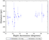 |
Fig. 2 Relation between distance and right ascension for the 30 sources in Table 2. |
| In the text | |
|
Fig. 3 Color-coded 2D visualisation of Eq. (1). Color bar is in parsec, coordinates grid in degrees. Black dashed lines connect points at the same distance, shown in the labels. The coordinates grid, in blue, is in steps of 2°. Green labels are the distances derived by Zucker et al. (2019) in boxes of 0.84 |
| In the text | |
|
Fig. 4 Top panel: column density map with contours at 3 × 1021 cm−2 and 1022 cm−2. Bottom panel: dust temperature map. In both panels, the magenta line in the bottom-left corner shows the angular scale corresponding to 1 pc at 300 pc; J2000.0 coordinates grid is shown. Both maps have a spatial resolution of 36′′. 1. The anticorrelation between N(H2) and Td is evident: regions at high/low column density are cold/warm, with few exceptions in IC348 and NGC 1333. |
| In the text | |
|
Fig. 5 Histogram of dust temperature in the range 11–21 K (minimum is 10.1 K, maximum is 28.3 K). |
| In the text | |
|
Fig. 6 Ratio of τH, the optical depth derived from our Herschel observations, to τP, the opticaldepth derived from Planck observations (Planck Collaboration XI 2014) (grey points), with both τ values computed at 850 μm. The ratio is plotted vs. τP. Green pointscorrespond to low values of τH due to the convolution applied to the Herschel column density map (see text). Mean values ± one standard deviation of the grey points, excluding the green ones, are shown with the blue histogram. The dark green and the two red lines show the weighted mean of the ratio: 1.174 ± 0.040. |
| In the text | |
|
Fig. 7 Left panel: inferred 70 μm intensity map extrapolated from the column density and temperature maps obtained for λ ≥ 160 μm. The green circle shows the bubble found by Ridge et al. (2006b) (CPS5 in the list by Arce et al. 2011). Right panel: difference between the observed 70 μm map and the extrapolated map. Green contours are 20 and 200 MJy sr−1; blue contours show the region where TPACSonly ≥ 20 K (see text). Colour bars are in MJy sr−1. |
| In the text | |
|
Fig. 8 Change in dust temperature when only PACS data are used (70, 100 and 160 μm) instead of PACS 160 μm plus SPIRE bands. Error bars are one standard deviation. The point at T ~ 30 K is not reliable because only a few values are available to compute the mean. |
| In the text | |
|
Fig. 9 Regions identified in Perseus overplotted on the column density map. The magenta line in the bottom left corner shows the angular scale corresponding to 1 pc at 300 pc. The J2000.0 coordinates grid is also shown. Coordinates of the regions are given in Appendix C. |
| In the text | |
|
Fig. 10 Network of filaments overplotted on the column density map. Red lines show the spine of the filaments, white lines show the branches, and the green contours show the width of the filaments and branches. The map has been rotated by 28°. The magenta line in the centre shows the angular scale corresponding to 1 pc at 300 pc. The J2000.0 coordinates grid is shown. |
| In the text | |
|
Fig. 11 Left panel: zoom-in of the filament in the region of L1448. The white line is the spine, while the grey line is the border of the filament. The short black lines are branches. To explain how the radial profile of the filament is derived, we defined, with the thick black line, an arbitrary region. Right panel: radial profile of the filament averaged longitudinally within the black region shown in the left panel. The error bars are the standard deviation of the column density averaged within ten pixels. The blue line is the Gaussian fit, and the grey line the estimated background. The dashed and dotted vertical lines are explained in the text. |
| In the text | |
|
Fig. 12 Histogram of the filament widths averaged over the spine (bin size 1 pixel or 0.02 pc at d = 300 pc). |
| In the text | |
|
Fig. 13 Histograms of mass per unit length for filaments with cores (green line) and prestellar cores (blue and red lines, see text). |
| In the text | |
|
Fig. 14 Column density PDF for the whole Perseus molecular cloud: s is the slope of the power-law fit, shown in red, over the interval x1–x2, both in 1021 cm−2. As shown with the green line, the fit can be extended down to ~4 × 1021 cm−2. The brownline is a log-normal fit to the low-density PDF whose parameters are given in the text. Note that N(H2) ~ 1.6 × 1021 cm−2 is the smallest column density having a closed contour in our map. |
| In the text | |
|
Fig. 15 Probability density functions for the subregions identified in Perseus where protostars were detected. In each panel, s gives the slope of the power-law fit, shown in red, in the interval delimited by x1 and x2, both in 1021 cm−2; the fitting procedure is detailed in the text. The x-axis is N(H2) in cm−2. Green lines extend the best fit over the interval of column densities where protostars were found (see Col. N(H2) in Table 9). |
| In the text | |
|
Fig. 16 Relation between mass and radius for all the 519 detected cores: vertical dashed line corresponds to 0.026 pc, the linear distance corresponding to the FWHM (18′′. 2) of the high-resolution column density map at 300 pc. The three power laws are fit to our data. Black triangles are hot starless cores discussed in the text; also the blue dashed line is discussed in the text. |
| In the text | |
|
Fig. 17 Relation between T and mean column density of the sources, where symbols are defined as in the previous figure. The two lines are linear fits of the form T = slogN(H2) + b. The slopes s are given inthe legend and in the text where we also report the uncertainties. Black triangles are hot starless cores discussed in the text. |
| In the text | |
|
Fig. 18 Relation between T and M of the sources. The warmest unbound source at ~40 K is not shown to limit the extension of the x-axis. Bound sources are shown in blue, unbound sources in green, and candidate bound sources in red. |
| In the text | |
|
Fig. 19 Core mass function (dN/d logM) for the 199 robust prestellar cores (blue histogram), and for the 299 robust and candidateprestellar cores (red histogram) in Perseus. The two distributions overlap above M ~ 1.2. Histogramsuse a bin size of logM = 0.1. Green and dashed grey lines show a log normal fit, and the orange line shows a power-lawfit (see text for details). The dashed black line shows the completeness limit at ~ 0.32 M⊙. |
| In the text | |
|
Fig. 20 Prestellar core mass function (dN/d logM) for sources in Perseus when each core is assigned a different distance based on Eq. (1). Lines as in Fig. 19. |
| In the text | |
|
Fig. 21 Left panel: comparison of robust bound cores and starless cores. Histograms with the y-axis on the left show the distributions of all starless cores (blue) and all bound cores (green). The red and black lines (right y-axis) show cumulative surface density distributions for all bound cores and the off-filament bound cores, respectively. These distributions were derived by dividing the number of cores found at a certain N(H2) level by the total area in the image where the density is below that value. Right panel: prestellar core mass vs. background N(H2). Triangles are the mean mass averaged over bins of 1021 cm−2. The linear fit is shown as a red line. |
| In the text | |
|
Fig. 22 Minimum distance between bound cores (blue), unbound cores (green), and tentative bound cores (red). |
| In the text | |
|
Fig. 23 Column density map overlaid with the positions of the 299 prestellar cores (yellow crosses and red crosses are robust and tentative cores, respectively), 220 unbound cores (blue hashes), and 132 protostars (cyan asterisks; we note that these sources were detected on the 70 μm map, which does not overlap completely with the SPIRE field of view, and so five cores are found outside the column density map). The map is rotated by 28°, with the top and bottom corners cut out. The magenta line in the centre shows the angular scale corresponding to 1 pc at 300 pc; J2000.0 coordinates grid is shown. |
| In the text | |
|
Fig. 24 Star formation efficiency as a function of the PDF slope for the different subclouds in Perseus, and for the whole cloud. The red point is an alternative SFE for Perseus (see text). The cyan line is a linear fit without taking into account uncertainties on the x-axis. |
| In the text | |
|
Fig. 25 Coreformation efficiency as a function of the power-law slope of the PDFs for the different subclouds in Perseus, and for the whole cloud. |
| In the text | |
|
Fig. 26 Distribution of free-fall time for robust prestellar cores. Top-axis is the uniform density for spherical cores (3M∕4πR3). The red lineis a Gaussian fit. |
| In the text | |
|
Fig. A.1 An example of the atlas of the Perseus cores showing the prestellar core #49. The original size of the page is A4, here thepage has been shrunk to one third. |
| In the text | |
|
Fig. A.2 An example of the atlas of the Perseus cores showing the protostar core #55. Also in this case the page has been shrunk. |
| In the text | |
|
Fig. A.3 Coordinates of source #55 at 250 μm as derived in the protostars (top) and starless cores (bottom) catalogues, respectively. |
| In the text | |
|
Fig. A.4 Effects on the SED when using an alternative extraction strategy (see text). Top panels: undetected and detected source at 160 μm. Bottom panels: SEDs with an upper limit and measure at 160 μm. |
| In the text | |
|
Fig. A.5 Effects on the SED when the measurement at 160 μm is used instead of the upper limit for undetected sources (see text). Left panel: best-fit with upper limit; right panel: best-fit witha measure. |
| In the text | |
|
Fig. B.1 Number of detected sources over number of simulated sources vs. true core mass. The completeness limit is defined as the mass at which completeness is 90%: in our case this happens at 0.323 M⊙, the limit shown as intersection between the two dashed lines. The decrease in the number of detected sources at high mass is discussed in the text (see also next figure). |
| In the text | |
|
Fig. B.2 Contrast level (see text) for detected sources (blue triangles) and undetected sources (red triangles). |
| In the text | |
|
Fig. C.1 Maps of 13CO in three velocity channels: 1.1 Km s−1 (top), 4.35 Km s−1 (centre), 6.0 Km s−1 (bottom); colour bars are uncorrected antenna temperature in K. Green labels mark the position of Gaia sources (see Table 2); h labels show the position of Hirota et al. (2008) and Hirota et al. (2011) sources (SVS13 is in the cloud of sources 6-10). The magenta lines at the centre of each map show the angular scale corresponding to 1 pc at 300 pc; J2000.0 coordinates grid is shown. |
| In the text | |
|
Fig. C.2 Maps of 13CO in three velocity channels: 7.9 Km s−1 (top), 8.8 Km s−1 (centre), 10.0 Km s−1 (bottom). In the latter panel, north of B5 and slightly covered by label 28, the bubble CPS12 (Arce et al. 2011) is evident. The magenta lines at the centre of each map show the angular scale corresponding to 1 pc at 300 pc; J2000.0 coordinates grid is shown. Labels as in Fig. C.1. |
| In the text | |
|
Fig. C.3 13CO spectra for all the subregions we defined in Perseus. Whenever possible we made a Gaussian fit to one or two profiles; forthe broad bumps we simply derived the position of the maximum and assigned it an uncertainty of 0.066 km s−1, which is equal to the step in the velocity grid. |
| In the text | |
|
Fig. D.1 Combined maps of Perseus at 70 μm (top, grid of equatorial J2000.0 coordinates, HPBW 8′′.4) and 160 μm (bottom, grid of Galactic coordinates, HPBW 13′′.5). Colour bars in MJy sr−1. |
| In the text | |
|
Fig. D.2 SPIRE intensity map of Perseus at 250 μm (top, grid of equatorial J2000.0 coordinates) and the high-resolution column density map (bottom, grid of Galactic coordinates). For both maps the HPBW is 18′′. 2. Colour bars are in MJy sr−1 (top) and cm−2 (bottom). |
| In the text | |
|
Fig. D.3 SPIRE intensity maps of Perseus at 350 μm (top, grid of Galactic coordinates, HPBW 24′′.9) and 500 μm (bottom, grid of ecliptic coordinates, HPBW 36′′.1). Colourbars in MJy sr−1. |
| In the text | |
Current usage metrics show cumulative count of Article Views (full-text article views including HTML views, PDF and ePub downloads, according to the available data) and Abstracts Views on Vision4Press platform.
Data correspond to usage on the plateform after 2015. The current usage metrics is available 48-96 hours after online publication and is updated daily on week days.
Initial download of the metrics may take a while.