| Issue |
A&A
Volume 571, November 2014
Planck 2013 results
|
|
|---|---|---|
| Article Number | A31 | |
| Number of page(s) | 25 | |
| Section | Cosmology (including clusters of galaxies) | |
| DOI | https://doi.org/10.1051/0004-6361/201423743 | |
| Published online | 29 October 2014 | |
Planck 2013 results. XXXI. Consistency of the Planck data
1
APC, AstroParticule et Cosmologie, Université Paris Diderot, CNRS/IN2P3,
CEA/lrfu, Observatoire de Paris, Sorbonne Paris Cité, 10 rue Alice Domon et Léonie Duquet,
75205
Paris Cedex 13,
France
2
Aalto University Metsähovi Radio Observatory and Dept of Radio
Science and Engineering, PO Box
13000, 00076
Aalto,
Finland
3
African Institute for Mathematical Sciences, ,
6-8 Melrose Road, 7945 Muizenberg,
Cape Town, South
Africa
4
Agenzia Spaziale Italiana Science Data Center, ,
Via del Politecnico snc,
00133
Roma,
Italy
5
Agenzia Spaziale Italiana, Viale Liegi 26, Roma, Italy
6
Astrophysics Group, Cavendish Laboratory, University of
Cambridge, J J Thomson
Avenue, Cambridge
CB3 0HE,
UK
7
Astrophysics & Cosmology Research Unit, School of Mathematics,
Statistics & Computer Science, University of KwaZulu-Natal, ,
Westville Campus, Private Bag
X54001, 4000
Durban, South
Africa
8
CITA, University of Toronto, 60 St. George St., Toronto, ON
M5S 3H8,
Canada
9
CNRS, IRAP, 9 Av.
Colonel Roche, BP
44346, 31028
Toulouse Cedex 4,
France
10
California Institute of Technology, Pasadena, California, USA
11
Centre for Theoretical Cosmology, DAMTP, University of
Cambridge, Wilberforce
Road, Cambridge
CB3 0WA,
UK
12
Computational Cosmology Center, Lawrence Berkeley National
Laboratory, Berkeley,
California,
USA
13
DSM/Irfu/SPP, CEA-Saclay, 91191
Gif-sur-Yvette Cedex,
France
14
DTU Space, National Space Institute, Technical University of
Denmark, Elektrovej
327, 2800
Kgs. Lyngby,
Denmark
15
Département de Physique Théorique, Université de
Genève, 24 quai E.
Ansermet, 1211
Genève 4,
Switzerland
16
Departamento de Física, Universidad de Oviedo, ,
Avda. Calvo Sotelo s/n,
33007
Oviedo,
Spain
17
Department of Astrophysics/IMAPP, Radboud University
Nijmegen, PO Box
9010, 6500 GL
Nijmegen, The
Netherlands
18
Department of Electrical Engineering and Computer Sciences,
University of California, Berkeley, California, USA
19
Department ofPhysics & Astronomy, University of British
Columbia, 6224 Agricultural Road,
Vancouver, British
Columbia, Canada
20
Department of Physics and Astronomy, Dana and David Dornsife College
of Letter, Arts and Sciences, University of Southern California, ,
Los Angeles, CA
90089,
USA
21
Department of Physics and Astronomy, University College
London, London
WC1E 6BT,
UK
22
Department of Physics, Florida State University, ,
Keen Physics Building, 77 Chieftan
Way, Tallahassee,
Florida,
USA
23
Department of Physics, Gustaf Hällströmin katu 2a, University of
Helsinki, 00014
Helsinki,
Finland
24
Department of Physics, Princeton University, ,
Princeton, New Jersey, USA
25
Department of Physics, University of California, ,
Santa Barbara, California, USA
26
Department of Physics, University of Illinois at
Urbana-Champaign, 1110 West Green
Street, Urbana,
Illinois,
USA
27
Dipartimento di Fisica e Astronomia G. Galilei, Università degli
Studi di Padova, via Marzolo
8, 35131
Padova,
Italy
28
Dipartimento di Fisica e Scienze della Terra, Università di
Ferrara, Via Saragat
1, 44122
Ferrara,
Italy
29
Dipartimento di Fisica, Università La Sapienza, ,
P.le A. Moro 2, 00185
Roma,
Italy
30
Dipartimento di Fisica, Università degli Studi di
Milano, via Celoria,
16, 20133
Milano,
Italy
31
Dipartimento di Fisica, Università degli Studi di
Trieste, via A. Valerio
2, 34127
Trieste,
Italy
32
Dipartimento di Fisica, Università di Roma Tor
Vergata, via della Ricerca Scientifica,
1, 00133
Roma,
Italy
33
Discovery Center, Niels Bohr Institute, Blegdamsvej 17, 2100
Copenhagen,
Denmark
34
Dpto. Astrofísica, Universidad de La Laguna (ULL), ,
38206, La Laguna, Tenerife,
Spain
35
European Space Agency, ESAC, Planck Science Office, Camino bajo del
Castillo, s/n, Urbanización
Villafranca del Castillo, 28691 Villanueva de la Cañada, Madrid, Spain
36
European Space Agency, ESTEC, Keplerlaan 1, 2201 AZ
Noordwijk, The
Netherlands
37
Finnish Centre for Astronomy with ESO (FINCA), University of
Turku, Väisäläntie
20, Piikkiö
21500,
Finland
38
Haverford College Astronomy Department, 370 Lancaster Avenue, Haverford, Pennsylvania, USA
39
Helsinki Institute of Physics, Gustaf Hällströmin katu 2, University
of Helsinki, 00014
Helsinki,
Finland
40
INAF – Osservatorio Astronomico di Padova, ,
Vicolo dell’Osservatorio 5,
35122
Padova,
Italy
41
INAF – Osservatorio Astronomico di Roma, ,
via di Frascati 33, 00040
Monte Porzio Catone,
Italy
42
INAF – Osservatorio Astronomico di Trieste, ,
via G.B. Tiepolo 11, 34143
Trieste,
Italy
43
INAF/IASF Bologna, via Gobetti 101, 40129
Bologna,
Italy
44
INAF/IASF Milano, via E. Bassini 15, 20133
Milano,
Italy
45
INFN, Sezione di Bologna, via Irnerio 46, 40126
Bologna,
Italy
46
INFN, Sezione di Roma 1, Università di Roma Sapienza, ,
P.le Aldo Moro 2, 00185
Roma,
Italy
47
INFN/National Institute for Nuclear Physics, ,
Via Valerio 2, 34127
Trieste,
Italy
48
IPAG: Institut de Planétologie et d’Astrophysique de Grenoble,
Université Joseph Fourier, Grenoble
1/CNRS-INSU, UMR 5274, 38041
Grenoble,
France
49
IUCAA, Post Bag 4, Ganeshkhind, Pune University
Campus, 411 007
Pune,
India
50
Imperial College London, Astrophysics group, Blackett
Laboratory, Prince Consort
Road, London,
SW7 2AZ,
UK
51
Infrared Processing and Analysis Center, California Institute of
Technology, Pasadena,
CA
91125,
USA
52
Institut Universitaire de France, 103 bd Saint-Michel, 75005
Paris,
France
53
Institut d’Astrophysique Spatiale, CNRS (UMR 8617) Université
Paris-Sud 11, Bâtiment
121, 91405
Orsay,
France
54
Institut d’Astrophysique de Paris, CNRS (UMR 7095), ,
98bis boulevard Arago,
75014
Paris,
France
55
Institute for Space Sciences, Bucharest-Magurale,
Romania
56
Institute of Astronomy, University of Cambridge, ,
Madingley Road, Cambridge
CB3 0HA,
UK
57
Institute of Theoretical Astrophysics, University of
Oslo, Blindern,
0315
Oslo,
Norway
58
Instituto Nacional de Astrofísica, Óptica y Electrónica
(INAOE), Apartado Postal 51 y
216, 72000
Puebla,
México
59
Instituto de Astrofísica de Canarias, C/Vía Láctea s/n, 38200, La
Laguna, Tenerife, Spain
60
Instituto de Física de Cantabria (CSIC-Universidad de
Cantabria), Avda. de los Castros
s/n, 39005
Santander,
Spain
61
Jet Propulsion Laboratory, California Institute of
Technology, 4800 Oak Grove
Drive, Pasadena,
California,
USA
62
Jodrell Bank Centre for Astrophysics, Alan Turing Building, School
ofPhysics and Astronomy, The University of Manchester, Oxford Road, Manchester, M13
9PL, UK
63
Kavli Institute for Cosmology Cambridge, ,
Madingley Road, Cambridge, CB3 0HA, UK
64
LAL, Université Paris-Sud, CNRS/IN2P3, Orsay, France
65
LERMA, CNRS, Observatoire de Paris, 61 avenue de l’Observatoire, 75014
Paris,
France
66
Laboratoire AIM, IRFU/Service d’Astrophysique – CEA/DSM – CNRS –
Université Paris Diderot, Bât. 709,
CEA-Saclay, 91191
Gif-sur-Yvette Cedex,
France
67
Laboratoire Traitement et Communication de l’Information, CNRS (UMR
5141) and Télécom ParisTech, 46 rue
Barrault, 75634
Paris Cedex 13,
France
68
Laboratoire de Physique Subatomique et de Cosmologie, Université
Joseph Fourier Grenoble I, CNRS/IN2P3, Institut National Polytechnique de
Grenoble, 53 rue des
Martyrs, 38026
Grenoble Cedex,
France
69
Laboratoire de Physique Théorique, Université Paris-Sud 11 &
CNRS, Bâtiment 210,
91405
Orsay,
France
70
Max-Planck-Institut für Astrophysik, Karl-Schwarzschild-Str. 1, 85741
Garching,
Germany
71
McGill Physics, Ernest Rutherford Physics Building, McGill
University, 3600 rue
University, Montréal,
QC, H3A 2T8, Canada
72
National University of Ireland, Department of Experimental
Physics, Maynooth,
Co. Kildare,
Ireland
73
Niels Bohr Institute, Blegdamsvej 17, 2100
Copenhagen,
Denmark
74
Observational Cosmology, Mail Stop 367-17, California Institute of
Technology, Pasadena,
CA, 91125, USA
75
SB-ITP-LPPC, EPFL, 1015, Lausanne, Switzerland
76
SISSA, Astrophysics Sector, via Bonomea 265, 34136
Trieste,
Italy
77
School of Physics and Astronomy, Cardiff University, ,
Queens Buildings, The Parade,
Cardiff, CF24 3AA, UK
78
School of Physics and Astronomy, University of
Nottingham, Nottingham
NG7 2RD,
UK
79
Space Sciences Laboratory, University of California, ,
Berkeley, California, USA
80
Special Astrophysical Observatory, Russian Academy of
Sciences, Nizhnij Arkhyz,
Zelenchukskiy region, 369167
Karachai-Cherkessian Republic,
Russia
81
Theory Division, PH-TH, CERN, 1211
Geneva 23,
Switzerland
82
UPMC Univ Paris 06, UMR7095, 98bis boulevard Arago, 75014
Paris,
France
83
Université de Toulouse, UPS-OMP, IRAP, 31028
Toulouse Cedex 4,
France
84
University of Granada, Departamento de Física Teórica y del Cosmos,
Facultad de Ciencias, 18071
Granada,
Spain
85
University of Granada, Instituto Carlos I de Física Teórica y
Computacional, Granada,
Spain
86
Warsaw University Observatory, Aleje Ujazdowskie 4, 00-478
Warszawa,
Poland
Received: 2 March 2014
Accepted: 29 July 2014
Abstract
The Planck design and scanning strategy provide many levels of redundancy that can be exploited to provide tests of internal consistency. One of the most important is the comparison of the 70 GHz (amplifier) and 100 GHz (bolometer) channels. Based on different instrument technologies, with feeds located differently in the focal plane, analysed independently by different teams using different software, and near the minimum of diffuse foreground emission, these channels are in effect two different experiments. The 143 GHz channel has the lowest noise level on Planck, and is near the minimum of unresolved foreground emission. In this paper, we analyse the level of consistency achieved in the 2013 Planck data. We concentrate on comparisons between the 70, 100, and 143 GHz channel maps and power spectra, particularly over the angular scales of the first and second acoustic peaks, on maps masked for diffuse Galactic emission and for strong unresolved sources. Difference maps covering angular scales from 8° to 15′ are consistent with noise, and show no evidence of cosmic microwave background structure. Including small but important corrections for unresolved-source residuals, we demonstrate agreement (measured by deviation of the ratio from unity) between 70 and 100 GHz power spectra averaged over 70 ≤ ℓ ≤ 390 at the 0.8% level, and agreement between 143 and 100 GHz power spectra of 0.4% over the same ℓ range. These values are within and consistent with the overall uncertainties in calibration given in the Planck 2013 results. We also present results based on the 2013 likelihood analysis showing consistency at the 0.35% between the 100, 143, and 217 GHz power spectra. We analyse calibration procedures and beams to determine what fraction of these differences can be accounted for by known approximations or systematicerrors that could be controlled even better in the future, reducing uncertainties still further. Several possible small improvements are described. Subsequent analysis of the beams quantifies the importance of asymmetry in the near sidelobes, which was not fully accounted for initially, affecting the 70/100 ratio. Correcting for this, the 70, 100, and 143 GHz power spectra agree to 0.4% over the first two acoustic peaks. The likelihood analysis that produced the 2013 cosmological parameters incorporated uncertainties larger than this. We show explicitly that correction of the missing near sidelobe power in the HFI channels would result in shifts in the posterior distributions of parameters of less than 0.3σ except for As, the amplitude of the primordial curvature perturbations at 0.05 Mpc-1, which changes by about 1σ. We extend these comparisons to include the sky maps from the complete nine-year mission of the Wilkinson Microwave Anisotropy Probe (WMAP), and find a roughly 2% difference between the Planck and WMAP power spectra in the region of the first acoustic peak.
Key words: cosmology: observations / cosmic background radiation / instrumentation: detectors
Corresponding author: C. R. Lawrence, e-mail: This email address is being protected from spambots. You need JavaScript enabled to view it.
© ESO, 2014
1. Introduction
This paper, one of a set associated with the 2013 release of data from the Planck1 mission (Planck Collaboration I 2014), describes aspects of the internal consistency of the Planck data in the 2013 release not addressed in the other papers. The Planck design and scanning strategy provide many levels of redundancy, which can be exploited to provide tests of consistency (Planck Collaboration I 2014), most of which are carried out routinely in the Planck data processing pipelines (Planck Collaboration II 2014; Planck Collaboration VI 2014; Planck Collaboration XV 2014; Planck Collaboration XVI 2014). One of the most important consistency tests for Planck is the comparison of the LFI and HFI channels, and indeed this was a key feature of its original experimental concept. Based on different instrument technologies, with feeds located differently in the focal plane, and analysed independently by different teams, these two instruments provide a powerful mutual assessment and test of systematic errors. This paper focuses on comparison of the LFI and HFI channels closest in frequency to each other and to the diffuse foreground minimum, namely the 70 GHz (LFI) and 100 GHz (HFI) channels2, together with the 143 GHz HFI channel, which has the greatest sensitivity to the cosmic microwave background (CMB) of all the Planck channels.
Quantitative comparisons involving different frequencies must take into account the effects of frequency-dependent foregrounds, both diffuse and unresolved. Planck processing for the 2013 results proceeds along two main lines, depending on the scientific purpose. For non-Gaussianity and higher-order statistics, and for the ℓ< 50 likelihood, diffuse foregrounds are separated at map level (Planck Collaboration XII 2014). Only the strongest unresolved sources, however, can be identified and masked from the maps, and the effects of residual unresolved foregrounds must be dealt with statistically. They therefore require corrections later in processing (e.g., Planck Collaboration XXIII 2014; Planck Collaboration XXIV 2014). For power spectra, the ℓ ≥ 50 likelihood, and parameters, both diffuse and unresolved source residuals are handled in the power spectra with a combination of masking and fitting of a parametric foreground model (Planck Collaboration XVI 2014).
In this paper, we compare Planck channels for consistency in two different ways. First, in Sects. 2 and 3, we compare frequency maps from the Planck 2013 data release – available from the Planck Legacy Archive (PLA)3 and referred to hereafter as PLA maps – and power spectra calculated from them, looking first at the effects of noise and foregrounds (both diffuse and unresolved), and then, in Sect. 4, at calibration and beam effects. This comparison based on publicly released maps ties effects in the data directly to characteristics of the instruments and their determination. This examination has provided important insights into our calibration and beam determination procedures even since the 2013 results were first released publicly in March 2013, confirming the validity of the 2013 cosmological results, resolving some issues that had been contributing to the uncertainties, and suggesting future improvements that will reduce uncertainties further.
Second, in Sect. 5, we compare power spectra again, this time from the “detector set” data at 100, 143, and 217 GHz (see Table 1 in Planck Collaboration XV 2014) used in the likelihood analysis described in Planck Collaboration XV (2014), but extending that analysis to include 70 GHz as well. These detector-set/likelihood comparisons give a measure of the agreement between frequencies in the data used to generate the Planck 2013 cosmological parameter results in Planck Collaboration XVI (2014). Taking into account differences in the data and processing, the same level of consistency is seen as in the comparison based on PLA frequency maps in Sect. 3. We then show that the small changes in beam window functions discussed in Sect. 4 have no significant effect on the 2013 parameter results other than the overall amplitude of the primordial curvature perturbations at 0.05 Mpc-1, As.
After having established consistency within the Planck data, specifically agreement between 70, 100, and 143 GHz over the first acoustic peak to better than 0.5% in the power spectrum, in Sect. 6 we compare Planck with WMAP, specifically the WMAP9 release4. The absolute calibration of the Planck 2013 results is based on the “solar dipole” (i.e., the motion of the Solar System barycentre with respect to the CMB) determined by WMAP7 (Hinshaw et al. 2009), whose uncertainty leads to a calibration error of 0.25% (Planck Collaboration V 2014). For the Planck channels considered in this paper, the overall calibration uncertainty is 0.6% in the 70 GHz maps and 0.5% in the 100 and 143 GHz maps (1.2% and 1.0%, respectively, in the power spectra; Planck Collaboration I 2014, Table 6). When comparing Planck and WMAP calibrated maps, however, one should remove from these uncertainties in the Planck maps the 0.25% contribution from the WMAP dipole, since it was the reference calibrator for both LFI and HFI. In the planned 2014 release, the Planck absolute calibration will be based on the “orbital dipole” (i.e., the modulation of the solar dipole due to the Earth’s orbital motion around the Sun), bypassing uncertainties in the solar dipole.
Throughout this paper we refer to frequency bands by their nominal designations of 30, 44, 70, 100, 143, 217, 353, 545, and 857 GHz for Planck and 23, 33, 41, 61, and 94 GHz for WMAP; however, we take bandpasses into account in all calculations. The actual weighted central frequencies determined by convolution of the bandpass response with a CMB spectrum are 28.4, 44.1, 70.4, 100.0, 143.0, 217.0, 353.0, 545.0, and 857.0 GHz for Planck, and 22.8, 33.2, 41.0, 61.4, and 94.0 GHz for WMAP. These correspond to the effective frequencies for CMB emission. For emission with different spectra, the effective frequency is slightly shifted.
The maps discussed in this paper are structured according to the HEALPix5 scheme (Górski et al. 2005) displayed in Mollweide projections in Galactic coordinates.
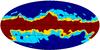 |
Fig. 1 Sky masks used for spectral analysis of the Planck 70, 100, and 143 GHz maps. The light blue, yellow, and red masks leave observable sky fractions fsky of 39.7%, 59.6%, and 69.4%, respectively, and are named GAL040, GAL060, and GAL070 in the PLA. These masks are extended by exclusion of unresolved sources in the PCCS 70, 100, and 143 GHz source lists above the 5σ flux density cuts. |
2. Comparison of frequency maps
The Planck 2013 data release includes maps based on 15.5 months of data, as well as maps of subsets of the data that enable tests of data quality and systematic errors. Examples include (see Planck Collaboration I 2014 for complete descriptions) single survey maps and half-ring difference maps, made by splitting the data from each pointing period of the satellite into halves, making separate sky maps from the two halves, and taking the difference of the two maps. Half-ring maps are particularly useful in characterizing the noise, and also enable signal estimation based on cross-spectra, with significant noise reduction compared to auto-spectra.
The 100 and 143 GHz maps are released at HEALPix resolution Nside = 2048, with
 pixels of approximately 1.́7. Although the
LFI maps are generally released at Nside = 1024, the 70 GHz maps are also
released at Nside =
2048. All mapmaking steps except map binning at the given pixel
resolution are the same for the two resolutions. In this paper we use the 70 GHz maps made
at Nside =
2048 for comparison with the 100 and 143 GHz sky maps.
pixels of approximately 1.́7. Although the
LFI maps are generally released at Nside = 1024, the 70 GHz maps are also
released at Nside =
2048. All mapmaking steps except map binning at the given pixel
resolution are the same for the two resolutions. In this paper we use the 70 GHz maps made
at Nside =
2048 for comparison with the 100 and 143 GHz sky maps.
2.1. Sky masks
Comparison of maps at different frequencies over the full sky is quite revealing of foregrounds, as will be seen. For most purposes in this paper we need to mask regions of strong foreground emission. We do this using the publicly-released6 Galactic masks GAL040, GAL060, and GAL070, shown in Fig. 1. These leave unmasked fsky = 39.7%, 59.6%, and 69.4% of the full sky. We mask unresolved (“point”) sources detected above 5σ in the 70, 100, and 143 GHz channels, as described in the Planck Catalogue of Compact Sources (PCCS; Planck Collaboration XXVIII 2014). The point source masks are circular holes centred on detected sources with diameter 2.25 times the FWHM beamsize of the frequency channel in question. The masks are unapodized, as the effect of apodization on large angular scales is primarily to improve the accuracy of covariance matrices.
2.2. Monopole/dipole removal
The Planck data have an undetermined absolute zero level, and the Planck maps contain low-amplitude offsets generated in the process of mapmaking, as well as small residual dipoles that remain after removal of the kinematic dipole anisotropy. We remove the ℓ = 0 and ℓ = 1 modes from the maps using χ2-minimization and the GAL040 mask, extended where applicable to a constant latitude of ± 45°. Diffuse Galactic emission at both low and high frequencies is still present even at high latitude, so this first step can leave residual offsets that become visible at the few microkelvin level in the difference maps smoothed to 8° shown in Appendix A. In those cases, a small offset adjustment, typically no more than a few microkelvin, is made to keep the mean value very close to zero in patches of sky visually clear of foregrounds.
2.3. Comparisons
Figure 2 shows the monopole- and dipole-removed maps at 70, 100, and 143 GHz, along with the corresponding half-ring difference maps. Figure 3 shows the difference maps between these three frequencies. The strong frequency-dependence of foregrounds is obvious. Equally obvious, and the essential point of the comparison, is the nearly complete nulling of the CMB anisotropies. This shows that these three channels on Planck are measuring the same CMB sky.
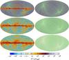 |
Fig. 2 Sky maps used in the analysis of Planck data consistency. Top row: 70 GHz. Middle row: 100 GHz. Bottom row: 143 GHz. Left column: signal maps. Right column: noise maps derived from half-ring differences. All maps are Nside = 2048. These are the publicly-released maps corrected for monopole and dipole terms as described in the text. The impression of overall colour differences between the maps is due to the interaction between noise, the colour scale, and display resolution. For example, the larger positive and negative swings between pixels in the 70 GHz noise map pick up darker reds and blues farther from zero. Smaller swings around zero in the 100 and 143 GHz noise maps result in pastel yellows and blues in adjacent pixels, which when displayed at less than full-pixel resolution give an overall impression of green, a colour not used in the colour bar. |
 |
Fig. 3 Difference maps. Top: 100 GHz minus 70 GHz. Middle: 143 GHz minus 100 GHz. Bottom: 143 GHz minus 70 GHz. All sky maps are smoothed to angular resolution FWHM = 15′ by a filter that accounts for the difference between the effective beam response at each frequency and a Gaussian of FWHM 15′. These maps illustrate clearly the difference in the noise level of the individual maps, excellent overall nulling of the CMB anisotropy signal, and frequency-dependent foregrounds. The 100–70 difference shows predominantly CO (J = 0 → 1) emission (positive) and free-free emission (negative). The 143–100 difference shows dust emission (positive) and CO emission (negative). The 143–70 difference shows dust emission (positive) and free-free emission (negative). The darker stripe in the top and bottom maps is due to reduced integration time in the 70 GHz channel in the first days of observation (see Planck Collaboration II 2014, Sect. 9.5). |
For a quantitative comparison, we calculate root mean square (rms) values of unmasked regions of the frequency and difference maps shown in Figs. 2 and 3, for the three masks shown in Fig. 1. To avoid spurious values caused on small scales by the differing angular resolution of the three frequencies, and on large scales by diffuse foregrounds, we first smooth the maps to a common resolution of 15′. We then smooth them further to 8° resolution, and subtract the 8° maps from the 15′ maps. This leaves maps that can be directly compared for structure on angular scales from 8° to 15′. We calculate rms values for half-ring sum (“Freq.”) and half-ring difference (“Diff.”) maps at 70, 100, and 143 GHz, and for the frequency-difference maps 70 GHz−100 GHz, 70 GHz−143 GHz, and 100 GHz−143 GHz. The rms values are given in Table 1. The maps are shown in Fig. A.1. Histograms of the frequency maps and difference maps are shown in Fig. 4.
 |
Fig. 4 Signal and noise for the frequency maps of Fig. 2 (left panel) and the difference maps of Fig. 3 (right panel), with the 59.6% mask in all cases. The broader, signal+noise curves are nearly Gaussian due to the dominant CMB anisotropies. The 70 GHz curve is broader than the 100 and 143 GHz curves because of the higher noise level, but is still signal-dominated for | dT/T | ≳ 50 μK. The narrower noise curves, derived from the half-ring difference maps, are not Gaussian because of the scanning-induced spatial dependence of pixel noise in Planck maps. The considerably higher noise level of the 70 GHz map is again apparent. The histograms of the difference maps show noise domination near the peak of each pair of curves (the signal+noise and noise curves overlap). The pairs involving 70 GHz are wider and dominated by the 70 GHz noise, but the wings at low pixel counts show the signature of foregrounds that exceed the noise levels, primarily dust and CO emission in the negative wing, and free-free and synchrotron emission in the positive wing. In the low-noise 100 minus 143 GHz pairs, the signal, due mostly to dust emission in the negative wing and to free-free and CO residuals in the positive wing, stands out clearly from the noise. |
Except for obvious foreground structures and noise, the difference maps lie close to zero, showing the excellent agreement between the three Planck frequencies for the CMB anisotropies.
The map comparisons give a comprehensive view of consistency between 70, 100, and 143 GHz, but the two-dimensional nature of the comparisons makes it somewhat difficult to grasp the key similarities. To make this easier, we turn now to comparisons at the power spectrum level.
3. Comparison of power spectra from 2013 results frequency maps
Power spectra of the unmasked regions of the maps are estimated as follows.
-
Starting from half-ring maps (Sect. 5.1 of PlanckCollaboration I 2014), cross-spectra arecomputed on the masked, incomplete sky using the HEALPixroutine anafast with ℓ = 0, 1 removal. These are so-called “pseudo-spectra”.
-
The MASTER spectral coupling kernel (Hivon et al. 2002), which describes spectral mode coupling on an incomplete sky, is calculated based on the mask used. The pseudo-spectra from the previous step are converted to 4π-equivalent amplitude using the inverse of the MASTER kernel.
-
Beam and pixel smoothing effects are removed from the spectra by dividing out the appropriate beam and pixel window functions. Beam response functions in ℓ space are required. We use the effective beam window functions derived using FEBeCoP (Mitra et al. 2011).
3.1. Spectral analysis of signals and noise
Figure 5 shows the signal (half-ring map cross-spectra), and noise (half-ring difference map auto-spectra) of the 70, 100, and 143 GHz channels. As stated earlier, the 70–100 GHz channel comparison quantifies the cross-instrument consistency of Planck.
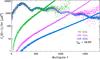 |
Fig. 5 Planck 70, 100, and 143 GHz CMB anisotropy power spectra computed
for the GAL060 mask. Mask- and beam-deconvolved cross-spectra of the half-ring maps
show the signal; auto-correlation spectra of the half-ring difference maps show the
noise. Points show single multipoles up to ℓ = 1200 for 70 GHz
and ℓ =
1700 for 100 and 143 GHz. Heavy solid lines show Δℓ = 20 boxcar
averages. The S/N near the first peak (ℓ = 220) is approximately 80, 1900, and 6000
for 70, 100, and 143 GHz, respectively. Noise power is calculated according to the
large-ℓ approximation, i.e., as a
|


![Mathematical equation: \hbox{$2 C_{\ell}^{\rm noise}[f_{\rm sky}(2\ell+1)]^{-1/2}$}](/articles/aa/full_html/2014/11/aa23743-14/aa23743-14-eq43.png)
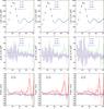 |
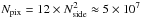
Fig. 6 Spectral analysis of the Planck 70, 100, and 143 GHz maps. Columns show results computed using the three sky masks in Fig. 1, with, from left to right, fsky = 69.4%, 59.6%, and 39.7%. Top row: CMB anisotropy spectra binned over a range of multipoles Δℓ = 40, for ℓ ≥ 30, with (2ℓ + 1)-weighting applied within the bin. Error bars are computed as a measure of the rms-power within each bin, and hence comprise both the measurement inaccuracy and cosmic variance. The grey curve is the best-fit Planck 6-parameter ΛCDM model from Planck Collaboration XVI (2014). Noise spectra computed from the half-ring-difference maps are shown: for the 70 GHz channel, the S/N ≈ 1 at ℓ ≈ 650. Middle row: residuals of the same power spectra with respect to the Planck best-fit model. Bottom row: power ratios for the 70 vs. 100 GHz and 143 vs. 100 GHz channels of Planck. The ratios are calculated ℓ by ℓ, then binned. The error bars show the standard error of the mean for the bin. The effect of diffuse foregrounds is clearly seen in the changes in the 143/100 ratio with sky fraction at ℓ ≈ 100. Bin-to-bin variations in the exact values of the ratios with sky fraction emphasize the importance of making such comparisons precisely. |
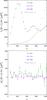 |
Fig. 7 Same as the top two panels of the middle column of Fig. 6, but without inclusion of signal cosmic variance in the uncertainties. Both signal × noise and noise × noise terms are included. |
This description of the statistics of noise contributions to the empirical cross-spectra derived from the Planck sky maps sets up the analysis of inter-frequency consistency of Planck data. The pure instrumental noise contribution to the empirical cross-spectra is very small over a large ℓ-range for the HFI channels, and at 70 GHz over the ℓ-range of the first peak in the spectrum, where we now focus our analysis. Cosmic variance is irrelevant for our discussion because we are assessing inter-frequency data consistency, and the instruments observe the same CMB anisotropy. Any possible departures from complete consistency of the measurements must be accounted for by frequency-dependent foreground emission, accurate accounting of systematic effects, or (at a very low level) residual noise.
3.2. Spectral consistency
Figure 6 shows spectra of the 70, 100, and 143 GHz maps for the three sky masks, differences with respect to the Planck 2013 best-fit model, and ratios of different frequencies. In the ℓ-range of the first peak and below, the 143/100 ratio shows the effects of residual diffuse foreground emission outside the masks. The largest mask reduces the detected amplitude, but does not remove it completely. The frequency dependence of the ratios conforms to what is well known, namely, that diffuse foreground emission is at a minimum between 70 and 100 GHz. The 143/100 pair is more affected by diffuse foregrounds than the 70/100 pair, as the dust emission gets brighter at 143 GHz. The effects of residual unresolved foregrounds in Fig. 6 are discussed in the next section.
Near the first acoustic peak, measurements in the three Planck channels agree to better than one percent of the CMB signal, and to much better than their uncertainties, which are dominated by the effects of cosmic/sample variance (see Fig. 6). Inclusion of cosmic/sample variance is essential for making inferences about the underlying statistical processes of the Universe; however, since the receivers at all frequencies are observing a single realization of the CMB, cosmic variance is irrelevant in the comparison of the measurements themselves. Figure 7 is the same as the top two middle panels of Fig. 6 (i.e., over 60% of the sky), but without inclusion of cosmic/sample variance in the uncertainties. As can be seen, cosmic/sample variance completely dominates the measurement uncertainties up to multipoles of 400, after which noise dominates.
3.3. Residual unresolved sources
Figure 6 shows that while diffuse foregrounds are significant for low multipoles, they are much less important on smaller angular scales. To see clearly the intrinsic consistency between frequencies, however, we must remove the effects of unresolved sources.
Discrete extragalactic foregrounds comprise synchrotron radio sources, Sunyaev-Zeldovich (SZ) emission in clusters, and dust emission in galaxies. These have complicated behaviour in ℓ and ν. All have a Poisson part, but the SZ and cosmic infrared background sources also have a correlated part. These are the dominant foregrounds (for a 39.7% Galactic mask) for ℓ ≳ 200. For frequencies in the range 70–143 GHz and multipoles in the range 50–200, they stay below 0.2%. The minimum in unresolved foregrounds remains at 143 GHz, with less than 2% contamination up to ℓ = 1000.
Discrete sources detected above 5σ in the PCCS (Planck Collaboration XXVIII 2014) are individually masked, as described in Sect.
2. Corrections for residual unresolved radio
sources are determined by fitting the differential Euclidean-normalized number counts
S5/2dN/dS in Jy1.5 sr-1 at each frequency with a
double power law plus Euclidean term:
![Mathematical equation: \begin{equation} S^{5/2}\,{\rm d}N/{\rm d}S = {A_{\rm f} S^{5/2} \over \left[ (S/S_1)^{b_{\rm f1}} + (S/S_2)^{b_{\rm f2}}\right] + A_{\rm E} \, (1 - {\rm e}^{-S/S_{\rm E}})}, \end{equation}](/articles/aa/full_html/2014/11/aa23743-14/aa23743-14-eq58.png) (1)where Af is the
amplitude at faint flux density levels, S1 is the first faint flux density
level, bf1 is the exponent of the first power law
at faint flux densities, S2 is the second faint flux density
level, bf2 is the exponent of the second power
law at faint flux densities, AE is the amplitude of the Euclidean
part, i.e., at large flux density, and SE is the flux density level for the
Euclidean part (≳ 1 Jy). These
are then integrated from a cutoff flux density corresponding to the 5σ selection limit in the
PCCS at 143 GHz, and the equivalent levels for a radio source with S ∝
ν-0.7 at 100 and 70 GHz. Thermal SZ and CIB
fluctuations are fitted as part of likelihood function determination described in Planck Collaboration XV (2014); the values found there
are used here. Figure 8 shows the level of these
corrections, while Fig. 9 shows the ratios of power
spectra after the corrections are made.
(1)where Af is the
amplitude at faint flux density levels, S1 is the first faint flux density
level, bf1 is the exponent of the first power law
at faint flux densities, S2 is the second faint flux density
level, bf2 is the exponent of the second power
law at faint flux densities, AE is the amplitude of the Euclidean
part, i.e., at large flux density, and SE is the flux density level for the
Euclidean part (≳ 1 Jy). These
are then integrated from a cutoff flux density corresponding to the 5σ selection limit in the
PCCS at 143 GHz, and the equivalent levels for a radio source with S ∝
ν-0.7 at 100 and 70 GHz. Thermal SZ and CIB
fluctuations are fitted as part of likelihood function determination described in Planck Collaboration XV (2014); the values found there
are used here. Figure 8 shows the level of these
corrections, while Fig. 9 shows the ratios of power
spectra after the corrections are made.
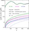 |
Fig. 8 Estimates of the residual thermal SZ and unresolved radio and infrared source residuals that must be removed. |
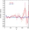 |
Fig. 9 Same as the bottom middle panel of Fig. 6, but corrected for differences in unresolved-source residuals (see text). We have not tried to account for uncertainties in the foreground correction itself; however, since the correction is small, the effect on the uncertainties would be small. |
3.4. Assessment
The 70/100 and 143/100 ratios in Fig. 9, for 59.6% of the sky, averaged over the range 70 ≤ ℓ ≤ 390 where the 70 GHz signal-to-noise ratio (S/N) is high, are 1.0080 and 1.0045, respectively. Over the range 70 ≤ ℓ ≤ 830, the ratios are 1.0094 and 1.0043, respectively. Table 2 collects these ratios and following ones for easy comparison.
Section 7.4 of Planck Collaboration VI (2014) uses the SMICA code to intercalibrate on the common CMB anisotropies themselves, with results given in Fig. 35 of that paper. For 40% of the sky, the 70/100 and 143/100 power ratios are 1.006 and 1.002 over the range 50 ≤ ℓ ≤ 300, and 1.0075 and 1.002 over the range 300 ≤ ℓ ≤ 700. (These gain ratios from Fig. 35 of Planck Collaboration VI 2014 must be squared for comparison with the power ratios discussed in this section and given in Table 2.) The SMICA equivalent power ratios are systematically about 0.2% closer to unity than those calculated in this section; however, in broad terms the two methods give remarkably similar results. Moreover, the absolute gain calibration uncertainties given in Planck Collaboration V (2014, Table 8) and Planck Collaboration VIII (2014) are 0.62% for 70 GHz and 0.54% for 100 GHz and 143 GHz. The agreement at the power spectrum level between 70, 100, and 143 GHz is quite reasonable in terms of these overall uncertainties. We will return to comparisons of spectra in Sects. 4 and 5.
Summary of ratios of Planck 70, 100, and 143 GHz power spectra appearing in this paper.
We are working continuously to refine our understanding of the instrument characteristics, implement more accurate calibration procedures, and understand and control systematic effects better. All of these will lead to reduced errors and uncertainties in 2014. In the next section we describe an analysis of beams and calibration procedures that has already been beneficial.
4. Beams, beam transfer functions, and calibration
The residual differences that we see in Sect. 3 are small but not negligible. We now address the question of whether they may be due to beam or calibration errors. Detailed descriptions and analyses of the LFI and HFI beams and calibration are contained in Planck Collaboration IV (2014), Planck Collaboration V (2014), Planck Collaboration VII (2014), and Planck Collaboration VIII (2014). In this section we summarize our present understanding of calibration and beam effects for the two instruments, explain the reasons for the approximations that have been made in data processing, provide estimates for the impact of these approximations on the resulting maps and power spectra, and outline plans for changes to be implemented in the 2014 data release. We will show that the small differences between LFI and HFI at intermediate ℓ seen in Fig. 9 are significantly reduced by improvements in our understanding of the near sidelobes in HFI, which affect the window functions in this ℓ range.
4.1. Beam definitions
Calibration of the CMB channels (30 to 353 GHz) is based on the dipole anisotropies produced by the motion of the Sun relative to the CMB and of the modulation of this dipole by the motion of the spacecraft relative to the Sun (which we refer to as the solar and orbital dipoles, respectively). For the 2013 data release and all LFI and HFI frequency channels considered in this paper, the time-ordered data have been fit to the solar dipole as measured by WMAP (Hinshaw et al. 2009). The present analysis aims to show that the LFI-HFI differences at intermediate ℓ seen in Fig. 9 are understood within the present uncertainties due to beams, calibration, and detector noise. Planck Collaboration IV (2014) and Planck Collaboration VII (2014) define three regions of the beam response (see Fig. 10, Fig. 1 of Planck Collaboration IV 2014, and Fig. 5 of Tauber et al. 2010), as follows.
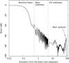 |
Fig. 10 Radial slice through a 70 GHz beam from the GRASP model, illustrating the nominal beam, near sidelobe, and far sidelobe regions. The exact choice of angular cutoff for the nominal beam is different for different frequencies. |
The nominal beam or main beam is that portion used to create the beam window functions for the 2013 data release. The nominal beam carries most of the beam shape information and more than 99% of the total solid angle, and therefore has most of the information needed for the 2013 cosmological analysis. The angle from the beam centre to the boundary of the nominal beam varies with frequency and instrument, and is 1.̊9, 1.̊3, and 0.̊9 for 30, 44, and 70 GHz, respectively, and 0.̊5 for 100 GHz and above.
The near sidelobes comprise any effective solid angle within 5° of the centre of the beam that is not included in the nominal beam. The response to the dipole from this region of the beam is very similar to that from the nominal beam, and unaccounted-for near sidelobe response leads to errors in the window function.
The far sidelobes comprise the beam response more than 5° from the centre. Because of the geometry of the telescope and baffles, the bulk of this solid angle is at large angles from the line of sight, not far from the spin axis, and not in phase with the dipole seen in the nominal beam, and therefore has little effect on the dipole calibration. However, the secondary mirror spillover, containing typically 1/3 of the total power in the far sidelobes, is in phase with the dipole, and affects the calibration signal. The inaccuracy introduced by approximating the optical response with the nominal beam normalized to unity is corrected to first order by our use of a pencil (δ-function) beam to estimate the calibration.
For reference, for the 2013 release we estimated a contribution to the solid angle from near sidelobes of 0.08%, 0.2%, and 0.2%, and from far sidelobes of 0.62%, 0.33%, and 0.31%, for 70, 100, and 143 GHz, respectively, of which 0.12%, 0.075%, and 0.055% is from the secondary spillover referred to above. Recent analysis, detailed in Appendix C, has resulted in a new estimate for the near sidelobe contribution for 100 and 143 GHz of 0.30 ± 0.2% and 0.35 ± 0.1%, respectively7. The impact of this is described below.
4.2. Nominal beam approximation
In the 2013 analysis, both LFI and HFI performed a “nominal beam” calibration, i.e., we
assumed that the detector response to the dipole can be approximated by the response of
the nominal beam alone, which in turn is modelled as a pencil beam (for details see
Appendix B). Clearly, if 100% of the power were
contained in the nominal beam, the window function would fully account for beam effects in
the reconstructed map and power spectrum. In reality, however, a fraction of the beam
power is missing from the nominal beam and appears in the near and far sidelobes,
affecting the map and power spectrum reconstruction in ways that depend on the level of
coupling of the sidelobes with the dipole. Accordingly, a correction factor is applied
that has the form (see Eq. (B.12))
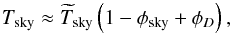 (2)where Tsky is the true
sky temperature,
(2)where Tsky is the true
sky temperature,  is the sky temperature estimated by the
“nominal beam” calibration, φD ≡
(Pside ∗
D)/(Pnominal ∗
D) is the coupling of the (near and far) sidelobes
with the dipole, and
is the sky temperature estimated by the
“nominal beam” calibration, φD ≡
(Pside ∗
D)/(Pnominal ∗
D) is the coupling of the (near and far) sidelobes
with the dipole, and 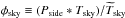 is a small term (of order 0.05%, see
Appendix C) representing the sidelobe coupling with
all-sky sources other than the dipole (mainly CMB anisotropies and Galactic emission). The
term φD is potentially
important, since dipole signals contributing to the near sidelobes may bias the dipole
calibration. Our current understanding of the value and uncertainty of the scale factors
η = (1 −
φsky +
φD) for LFI
and HFI is discussed in detail in Appendix C.
is a small term (of order 0.05%, see
Appendix C) representing the sidelobe coupling with
all-sky sources other than the dipole (mainly CMB anisotropies and Galactic emission). The
term φD is potentially
important, since dipole signals contributing to the near sidelobes may bias the dipole
calibration. Our current understanding of the value and uncertainty of the scale factors
η = (1 −
φsky +
φD) for LFI
and HFI is discussed in detail in Appendix C.
4.3. Key findings
There are two key findings or conclusions from the analyses in Appendices B and C.
-
For LFI, a complete accounting of the corrections using thecurrent full 4π beam model would lead to an adjustment of about 0.1% in the amplitude of the released maps (i.e., 0.2% of the power spectra). At present this is an estimate, and rather than adjusting the maps we include this in our uncertainty.
-
For HFI, recent work on a hybrid beam profile, including data from planet measurements and GRASP8 modelling, has led to improvements in the beam window function correction rising from 0 to 0.8, 0.8, 0.5, and 1.2% over the range ℓ = 1 to ℓ = 600, at 100, 143, 217, and 353 GHz, respectively. Uncertainties in these corrections have not been fully characterized, but are dominated by the intercalibration of Mars and Jupiter data and are comparable to the corrections themselves (see Fig. C.3).
Figure 11 shows the corrections to the beam window functions at 100, 143, and 217 GHz. Figure 12 shows the effect of those corrections on the 70/100 and 143/100 power spectrum ratios, uncorrected for unresolved source residuals. There is almost no effect on the 100/143 GHz ratio, as the differential beam window function correction between these two frequencies is small. The 70/100 ratio, however, is significantly closer to unity. In Sect. 5, we show that such a correction does not materially affect the 2013 cosmology results.
Figure 13 shows the power spectrum ratios corrected for both the beam window functions and unresolved source residuals (Sect. 3.3). The average ratios over the range 70 ≤ ℓ ≤ 390 are 1.0043 and 1.0046 for 70/100 and 143/100, respectively. For the range 70 ≤ ℓ ≤ 830, they are 1.0032 and 1.0043.
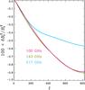 |
Fig. 11 Effective beam window function corrections from Fig. C.3, which correct for the effect of near-sidelobe power missing in the HFI beams used in the 2013 results (Sect. C.2.1). Uncertainties are not shown here for clarity, but are shown in Fig. C.3, and would be large on the scale of this plot. The 217 GHz correction is shown for illustration only. |
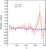 |
Fig. 12 Same as the bottom middle panel of Fig. 6, but corrected for the near-sidelobe power at 100 and 143 GHz that was not included in the 2013 results. Since the beam corrections for 100 and 143 GHz are nearly identical, the ratio 143/100 hardly changes. The ratio 70/100, however, changes significantly, moving towards unity. Uncertainties in the beam window function corrections are not included. |
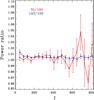 |
Fig. 13 Same as the bottom middle panel of Fig. 6, but corrected for both the near-sidelobe power at 100 and 143 GHz that was not included in the 2013 results and for unresolved source residuals (Sect. 3.3). Uncertainties in the beam window function corrections are not included. |
For the 2014 release, we expect internal consistency and uncertainties to further improve as more detailed models of the beam and correction factors are included in the analysis.
We have concentrated in this section on beam effects; however, the transfer function depends also on the residuals of the time transfer function, measured on planets and glitches, and deconvolved in the time-ordered data prior to mapmaking and calibration. For the HFI channels, the transfer function used for the 2013 cosmological analysis assumes that all remaining effects are contained within a 40′× 40′ map of a compact scanning beam and corresponding effective beam. Any residuals from uncorrected time constants longer than 1 s are left in the maps, and will affect the dipoles and thus the absolute calibration. This has been investigated since the 2013 data release; time constants in the 1–3 s range have been identified and shown to be the origin of difficulties encountered with calibration based on the orbital dipole. The 2014 data release will include a correction of these effects, and the absolute calibration will be carried out on the orbital dipole. A reduction in calibration uncertainties by a factor of a few can be anticipated.
5. Likelihood analysis
In the previous section we showed how work since release of the 2013 Planck results has led to an improved understanding of the beams and a small (and well within the stated uncertainties) revision to the near-sidelobe power in the HFI beams, which brings HFI and LFI into even closer agreement. In this section, we show that the revision in the HFI beams has little effect on cosmological parameters. To do this, we make use of the likelihood and parameter estimation machinery described in Planck Collaboration XV (2014) and Planck Collaboration XVI (2014). For both analytical and historical reasons there are differences (e.g., masks, frequencies, multipole ranges) in the analyses in this section and in previous sections; however, as will be seen, the effects of the differences are accounted for straightforwardly, and do not affect the conclusions about parameters.
The Planck 2013 cosmological parameter results given in Planck Collaboration XVI (2014) are determined for ℓ ≥ 50 from 100, 143, and 217 GHz “detector set” data described in Planck Collaboration XV (2014, Table 1), by means of the CamSpec likelihood analysis described in the same paper that solves simultaneously for calibration, foreground, and beam parameters. This approach allows power spectrum comparisons to sub-percent level precision, using only cross-spectra (as in Sect. 3) to avoid the need for accurate subtraction of noise in auto-spectra.
In this section, we determine the ratios of the 100, 143, and 217 GHz spectra using this approach, and compare the 143/100 results to those found in Sect. 3. We show that the apparent difference in the results from the two different approaches is easily accounted for by differences in the sky used, the difference between the detector set data and full frequency channel data, and the use of individual detector recalibration factors in the detector set/likelihood approach. Having established essentially exact correspondence between the methods, we use the likelihood machinery to estimate the effect on cosmological parameters of the revision in the near-sidelobe power in the HFI beams.
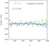 |
Fig. 14 Ratios of 100, 143, and 217 GHz power spectra calculated from detector sets with the likelihood method, including subtraction of the best-fitting foreground model (see text) and correction for the best-fit relative calibration factors for individual detectors. Solid symbols and lines show ratios for mask G22; open symbols and dotted or dashed lines show ratios for mask G35. The greater scatter in 217/143 for mask G35 is caused by CMB-foreground cross-correlations. |
In Planck Collaboration XVI (2014), we used mask G45 (fsky = 0.45) for 100 × 100 GHz, and mask G35 (fsky = 0.37) for 143 × 143 GHz and 217 × 217 GHz to control diffuse foregrounds. However, here we are interested in precise tests of inter-frequency power spectrum consistency, so (as before) we need to compute spectra using exactly the same masks to cancel the effects of cosmic variance from the primordial CMB. We have therefore recomputed all of the spectra using mask G22 (fsky = 0.22) and mask G35, restricting the sky area to reduce the effects of Galactic dust emission at 143 and 217 GHz. The spectra are computed from means of detector set cross-spectra Planck Collaboration XV (2014). For each spectrum, we subtract the best-fitting foreground model from the Planck+WP+high-ℓ solution for the base six-parameter ΛCDM model with parameters as tabulated in Planck Collaboration XVI (2014), and correct for the best-fit relative calibration factors of this solution. The convention adopted in the CamSpec likelihood fixes the calibration of 143 × 143 to unity, hence calibration factors multiply the 100 × 100 and 217 × 217 power spectra to match the 143 × 143 spectrum. The best fit values of these coefficients are c100 = 1.00058 and c217 = 0.9974 for mask G22, both very close to unity and consistent with the calibration differences between individual detectors at the same frequency (see Table 3 of Planck Collaboration XV 2014). The results are shown in Fig. 14.
The 143/100 ratio given by the dashed green line can be compared with the bottom right panel of Fig. 6, which is based on 40% of the sky, nearly the same as mask G35. As expected, they are not identical; Fig. 15 explains the differences. In Fig. 15, pairs of curves in the same colour show the difference between mask G22 and mask G35, as labelled. The cyan curves can be compared to the green curves in Fig. 14, which also have inter-frequency calibration and foreground corrections applied. The red curves show the effect of turning off detector-by-detector intercalibration. The blue curves show the effect of switching from detector sets to full-frequency half-ring cross spectra (as in Sect. 3). The progression from solid cyan to dashed blue in Fig. 15 shows the relationship between the PLA map-based results and the detector-set/likelihood results. As used in the likelihood analysis (Planck Collaboration XV 2014), the 143/100 ratio is 1.00058 over the full ℓ range used in the likelihood analysis, compared to the ratios between 1.0039 and 1.0046 seen in Table 2 over 70 ≤ ℓ ≤ 390 for Figs. 6, 9, 12, or 13. However, using mask G35 (fsky = 0.37), using half-ring cross-spectra of full-frequency detector sets, and turning off unresolved-source residual and detector-by-detector intercalibration factors, changes the ratio over 60 <ℓ< 390 to 1.0033, in good agreement with the 1.0039 calculated for the 143/100 comparison in the bottom right panel of Fig. 6.
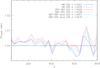 |
Fig. 15 Effects on the 143/100 ratio of changes in the mask, choice of detectors, and detector recalibration. Solid lines indicate ratios calculated with mask G22; dashed lines indicate mask G35. Use of detector sets gives the cyan curves with recalibration turned on and the red curves with recalibration turned off. Use of full-frequency half-ring cross spectra, as in Sect. 3, gives the blue curves. The cyan curves are comparable to the green curves in Fig. 14, which also have intra-frequency calibration and foreground corrections applied. The blue-dashed curve agrees extremely well with the blue curve in the bottom right panel of Fig. 6, as it should (see text). |
This agreement extends to the detailed shapes of the two curves (blue in the bottom right panel of Fig. 6 and blue-dashed in Fig. 15) as well. This is necessarily the case, since they are both cross-spectra of half-ring frequency maps, without corrections for unresolved-source residuals, and using the “2013” beams. The only difference in the data comes from the masks used, which are the GAL040 mask (fsky = 39.7%) and mask G35 (fsky = 37%), respectively. This agreement is nevertheless reassuring in showing that the differences in spectral ratios between the PLA map-based approach and the detector set likelihood approach are well-understood, and disappear for common data and masks.
We can now turn to the question of whether the small revision to the HFI beams affects cosmological parameters. A full revised beam analysis at the detector level that includes the 0.1% power in near sidelobes not taken into account directly in the 100 and 143 GHz beams in 2013 (Sect. 4) has not yet been completed; however, for an indicative test, we rescaled the averaged cross-spectra appearing in the likelihood by functions corresponding to the new beam shapes for the ℓ-ranges for which they have been calculated (presently up to ℓ = 2000). Where necessary the shapes were extrapolated as being flat up to higher ℓ. The 143 × 217 spectrum was rescaled by the geometric mean of the 143 and 217 rescalings. Then we performed a Monte Carlo Markov Chain (MCMC) analysis for the base ΛCDM model for the modified “high-ℓ” likelihood with an unmodified low-ℓ Planck likelihood and WMAP low-ℓ polarized likelihood (“WP”). To see any change in the beam error behaviour, we choose to sample explicitly over all twenty of the eigenmode amplitudes, rather than sampling over one and marginalizing over the other nineteen, as we did in the parameters paper (Planck Collaboration XVI 2014).
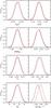 |
Fig. 16 Changes in cosmological parameters from the inclusion of the near sidelobe power discussed in the text. The black curves are the 2013 results for Planck plus the low-ℓ WMAP polarization (WP). The red curves are for Planck+WP using the revised HFI beams. The shifts in the posteriors are all less than 0.3σ except for the cosmological amplitude As and parameters related to it, as expected. |
The results are indicated in Figs. 16 and 17, showing a selection of cosmological parameters and the beam eigenmode amplitudes, respectively. As expected, we see a boost in the power spectrum amplitude, resulting in a change to the cosmological amplitude at about the 1σ level. However, the largest shift in any other cosmological parameter is 0.3σ. The uncertainty in the beam window function is described by a small number of eigenmodes in multipole space and their covariance matrix (Planck Collaboration VII 2014). The posteriors for the first beam eigenmodes for the 100, 143, and 217 effective spectra shift noticeably; others are practically unchanged. The beams used here are preliminary and the beam eigenmodes have not been generated self-consistently to match the beam calibration pipeline. No adjustment was made in the calibration of the low-ℓ likelihood. Nevertheless, from the results presented here, we can anticipate that the 2014 revisions to the beams will affect the overall calibration of the spectra, but will have little other impact on cosmology.
 |
Fig. 17 Changes in the beam eigenmode coefficients from the inclusion of the near-sidelobe power now established but not included in the processing for the 2013 results. Black curves are for Planck+WP; red curves are for Planck+WP with the revised beams. The superscript indicates the effective spectum (one to four for 100, 143, 217, and 143 × 217 respectively) while the subscript indicates eigenmode number. |
6. Comparison of Planck and WMAP
Planck and WMAP have both produced sky maps with excellent large-scale stability, as demonstrated by many null tests both internal to the data and external. In this section, we compare Planck and WMAP measurements in several different ways. In Sect. 6.1, we compare power spectra calculated from 70 and 100 GHz Planck maps available in the PLA, and from V- and W-band yearly maps in the WMAP9 data release. In Sect. 6.2, we perform a likelihood analysis similar to that in Sect. 5 and in Planck Collaboration XVI (2014), and show that the differences between the map-based and likelihood analyses are well-understood. In Sect. 6.3 we assess the results in the context of the uncertainties for the two experiments.
6.1. Map and power spectrum analysis
The WMAP9 data release includes Nside = 1024 yearly sky maps from individual differential assemblies (DAs), both corrected for foregrounds and uncorrected, as well as Nside = 512 frequency maps. WMAP uses somewhat different sky masks than Planck. In Sect. 3 we emphasized the importance of using exactly the same masks in comparing results. Accordingly, for Planck/WMAP comparisons we construct a joint mask, taking the union of the Planck GAL060 mask used in Sects. 3 and 4, the WMAP KQ85 mask, which imposes larger cuts for radio sources and some galaxy clusters, as required by the poorer angular resolution of WMAP, and the Planck joint 143, 100, 70 GHz point source mask. Fig. 18 shows the mask, which leaves fsky = 56.7% of the sky available for spectral analysis.
We use the same spectrum estimation procedure as in Sect. 3, evaluating the relevant cross-spectra, correcting for the mask with the appropriate kernel, and dividing out the relevant beam response and pixel smoothing functions. As the mask is different from the one used for Planck-only comparisons, so is the mask-correction kernel. All maps are analysed using the same mask.
For WMAP, there are nine yearly sky maps for each differential assembly V1, V2, W1, W2, W3, and W4, at Nside = 1024. Because the WMAP V band and the Planck 70 GHz band are so close in frequency, as are W band and 100 GHz, we use maps not corrected for foregrounds for the comparison. All possible cross spectra from the yearly maps and differential assemblies are computed (630 at W band, 153 at V), and corrected for the mask, beam (using WMAP beam response functions, different for each differential assembly), and pixel-smoothing. The corrected spectra are averaged, and the error on the mean is computed for each Cℓ. These average differential-assembly spectra are then co-added with inverse noise weighting to form one V band and one W band spectrum. These are binned (ℓmin = 30, Δℓ = 40), and rms errors in the bin values are computed. The resulting spectra are shown in Fig. 19.
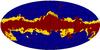 |
Fig. 18 Planckfsky ≈ 60% Galactic mask in yellow and WMAP KQ75 at Nside = 1024 in red. The mask used for comparative spectral analysis of the Planck 70, 100, and 143 GHz, and WMAP nine-year V- and W-band sky maps is the union of the two. The joint Planck 70, 100, and 143 GHz point source mask is also used, exactly as before. The final sky fraction is fsky = 56.7%. The Planck mask is degraded to the pixel resolution Nside = 1024, at which the yearly WMAP individual differential assembly maps are available. |
The 70, 100, and 143 GHz Planck spectra and spectral ratios in Figs. 19–21 are determined as before, but using the new mask, starting from the 70 GHz Nside = 1024 half-ring PLA maps and the 100 and 143 GHz Nside = 2048 maps degraded to Nside = 1024. Thus all spectra are evaluated with the identical mask, at the same resolution. Spectral binning and the estimation of rms bin errors proceed in exactly the same way as for the WMAP spectra and for previous Planck-only comparisons.
Figure 19 compares the Planck 70 GHz power spectrum with the WMAP V-band spectrum, and the Planck 100 GHz power spectrum with the WMAP W-band spectrum. The Planck 2013 best-fit model is shown for comparison. The Planck and WMAP9 spectra disagree noticeably in the ℓ-range of the first two peaks. Ratios of spectra in Fig. 20 show this disagreement directly. In Figs. 20–22 the 70/100 and 143/100 ratios are the same as in Sects. 3 and 4, except for the small change in the mask.
Figure 21 is the same as Fig. 20, but with the Planck 70/100 and 143/100 ratios corrected for the missing near sidelobe power in the 100 and 143 GHz channels, discussed in Sect. 4.
Figure 22 is the same as Fig. 21, but with all spectra additionally corrected for residual unresolved sources, as described in Sect. 3.3. Mean values of the ratios over specified multipole ranges are given in Table 3.
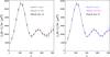 |
Fig. 19 Left: WMAP V band compared to Planck 70 GHz and best-fit model. Right: WMAP W band compared to Planck 100 GHz and best-fit model. The joint Planck/KQ75 sky mask + Planck point source mask (fsky = 56.7%; see Fig. 18) is used. Because the frequencies are so close, no corrections for foregrounds are made. |
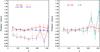 |
Fig. 20 Ratios of power spectra for Planck and WMAP over the joint Planck/KQ75+Planck point source mask with fsky = 56.7%. The Planck 70/100 and 143/100 ratios can be compared to the bottom middle panel in Fig. 6 for fsky = 59.6%. Here we limit the horizontal scale because the WMAP noise beyond ℓ = 400 makes the ratios uninformative. The general shape of the Planck ratios is the same; however, it is clear (as it was in Fig. 6) that changes in the sky fraction change the ratios significantly within the uncertainties. This underscores the importance of strict equality of all factors in such comparisons. |
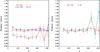 |
Fig. 21 Same as Fig. 20, but the Planck 70/100 and 143/100 ratios are corrected for beam power at 100 and 143 GHz that was not included in the effective beam window function used in the 2013 results. |
 |
Fig. 22 Same as Fig. 20, but including corrections for both Planck beams and for Planck and WMAP unresolved-source residuals. |
Summary of ratios of Planck 70 and 100 GHz and WMAP V- and W-band power spectra appearing in this paper.
6.2. Likelihood analysis
The likelihood analysis here is slightly different from the analysis presented in Sect. 5. First, we created a point source mask by concatenating the WMAP/70/100/143/217 point source catalogues. We present here only the results comparing WMAP, LFI 70 GHz, and HFI 100 GHz. Restricting the frequencies to a range close to the diffuse foreground minimum has the advantage that we can increase the sky area used. We therefore present results for mask G56 (unapodized), which leaves 56% of the sky. This mask, combined with the point source mask, is degraded in resolution from Nside = 2048 to the natural Nside for WMAP (512) and LFI (1024).
Beam-corrected spectra for the WMAP V, W, and V + W bands, and for the LFI 70 GHz bands were computed. Errors on these spectra were estimated from numerical simulations. At 70 GHz we have three maps of independent subsets of detectors, therefore we can estimate three pseudo-spectra by cross-correlating them by pairs. Pseudo-spectra are then mask- and beam-deconvolved. The final 70 GHz spectrum is obtained as a noise-weighted average of the cross-spectra. Noise variances are estimated from anisotropic, coloured noise MC maps for each set of detectors. We use the FEBeCoP effective beam window functions for each subset of detectors (the three pairs 18–23, 19–22, and 20–21 as defined in Planck Collaboration II 2014). In the present plots we do not show beam uncertainties, which are bounded to be ΔBℓ/Bℓ ≲ 0.2% in the multipole range considered here (Planck Collaboration VI 2014).
We also derive power spectra for the WMAP V and W bands, using coadded nine year maps per DA, for which no foreground cleaning has been attempted. There are two DA maps for V-band and four for W-band. The V-band spectrum is obtained by cross-correlating the two available maps, whereas the W spectrum is the noise-weighted average of the six spectra derived by correlating pairs of the four DA maps. We have produced Monte Carlo simulations of noise in order to assess the error bars of the WMAP spectra. We generate noise maps according to the pixel noise values provided by the WMAP team rescaled by the number of observations per pixel. Beam transfer functions per DA are those provided by the WMAP team. In the present error budget we did not include beam uncertainties, which would be ΔBℓ/Bℓ ≈ 0.4% for V and 0.5% for W, over ℓ< 400.
For LFI and WMAP, we subtract an unresolved thermal SZ template with the amplitude
derived from the CamSpec likelihood analysis, which we extrapolate to the central LFI and
WMAP frequencies. We also subtract a Poisson point source term with an amplitude chosen to
minimize the variance between the measured spectra and the best-fit theoretical model at
high multipoles. We then determine calibration factors cX for the WMAP and
70 GHz LFI spectrum relative to the 100 GHz HFI spectrum by minimizing 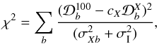 (3)until convergence, at each iteration
determining σI, an “excess scatter” term, by requiring
that the reduced χ2 be unity. (The excess scatter comes
primarily from foreground-CMB correlations, as discussed in Planck Collaboration XV 2014.) The sum extends over bins with central
multipole in the range 50 ≤ ℓ
≤ 400. The index X denotes the spectrum (70, V, W, or V + W),
and σXb is the noise
contribution to the error in band b. The spectra
(3)until convergence, at each iteration
determining σI, an “excess scatter” term, by requiring
that the reduced χ2 be unity. (The excess scatter comes
primarily from foreground-CMB correlations, as discussed in Planck Collaboration XV 2014.) The sum extends over bins with central
multipole in the range 50 ≤ ℓ
≤ 400. The index X denotes the spectrum (70, V, W, or V + W),
and σXb is the noise
contribution to the error in band b. The spectra
 in Eq. (3) are foreground-corrected.
Calibration factors cX and resulting
spectra for 70 GHz, V, W, and V + W-band relative to 100 GHz are
given in Fig. 23 and Table 3. The value of c70 = 0.994 seen in Fig. 23 is entirely consistent with the 70/100 ratios given
in Sect. 5, taking into account mask and dataset
variations as discussed in Sect. 5. A calibration
factor for V
relative to 70 GHz calculated the same way (
in Eq. (3) are foreground-corrected.
Calibration factors cX and resulting
spectra for 70 GHz, V, W, and V + W-band relative to 100 GHz are
given in Fig. 23 and Table 3. The value of c70 = 0.994 seen in Fig. 23 is entirely consistent with the 70/100 ratios given
in Sect. 5, taking into account mask and dataset
variations as discussed in Sect. 5. A calibration
factor for V
relative to 70 GHz calculated the same way ( is replaced by
 in Eq. (3)) is also included in Table 3.
To compare the likelihood results with the map-based ones, we need to identify the closest cases for which results are given. No correction for near sidelobes at 100 GHz (Sect. 4.3) was included in the likelihood results, but corrections for residual unresolved sources were. On the other hand, from the results shown in Table 3, residual-source corrections make negligible difference. In the likelihood approach, ℓ values beyond about 300 will be significantly down-weighted due to increased variance. Thus the most reasonable comparison is between the ratios from the map-based approach in the ℓ range 110 ≤ ℓ ≤ 310 with no corrections, and the corresponding calibration factors from the likelihood approach. Values in Table 3 show good agreement between the two analyses. We have furthermore noticed that using the WMAP full-mission maps at resolution Nside = 512 rather than the yearly maps at Nside = 1024, and Planck detector sets rather than full-frequency half-ring maps, can lower the spectral ratio by 0.2% in the multipole range 110 ≤ ℓ ≤ 310.
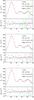 |
Fig. 23 Foreground-corrected spectra computed using mask G56, with calibration factors cX from Eq. (3) applied to 70 GHz, V, W, and V + W. The solid red lines in the upper panels show the best-fit model CMB spectrum (Planck Collaboration XVI 2014). The lower panels show the residuals with respect to this model. The error bars on the LFI and WMAP points show noise errors only. |
6.3. Assessment
Both the direct comparison of power spectra from the 2013 results maps and the likelihood analysis show a discrepancy between Planck and WMAP across the region of the first peak, where the S/N for WMAP is good. This difference is about 2% in power, corresponding to 1% in the maps. These numbers quantify what can be seen by eye in Fig. 19. The result is roughly the same for comparisons of 70 GHz with V-band and 100 GHz with W-band, where the frequency differences are small enough to rule out foregrounds as the cause. There is some variation of the ratio with ℓ (perhaps seen more easily in Fig. 23), suggesting that the cause is not simply a result of calibration errors, but neither does the shape correspond obviously to what would be expected from missing power in beams.
The 70/V and 100/W ratios differ from unity by more than expected from the uncertainties in absolute calibration determined for Planck and WMAP. Calibration of WMAP9 is based on the orbital dipole (i.e., the modulation of the solar dipole due to the Earth’s orbital motion around the Sun), with overall calibration uncertainty 0.2% (Bennett et al. 2013). The absolute calibration of the Planck 2013 results is based on the solar dipole (Sect. 1), assuming the WMAP5 value of (369.0 ± 0.9) km s-1, where the 0.24% uncertainty includes the 0.2% absolute calibration uncertainty (Hinshaw et al. 2009). The overall calibration uncertainty is 0.62% in the 70 GHz maps and 0.54% in the 100 and 143 GHz maps (Planck Collaboration I 2014, Table 6). When comparing Planck and WMAP calibrated maps, one must remove from these uncertainties the 0.2% contribution of the WMAP absolute calibration uncertainty to the WMAP dipole, which thus affects both LFI and HFI equally. The remaining 0.14% uncertainty in the WMAP dipole (mostly due to foregrounds; Hinshaw et al. 2009) affects Planck but not WMAP, because its absolute calibration is from the orbital dipole. In the planned 2014 release, the Planck absolute calibration will be based on the orbital dipole, bypassing uncertainties in the solar dipole. At the power spectrum level for comparison with WMAP, then, the Planck uncertainty would be between 2 × (0.54−0.2)% = 0.68% and 2 × (0.62−0.2)% = 0.84%, and the WMAP uncertainty 0.4%. The power spectrum ratios in Table 3 from Fig. 21 and Sect. 6.2 then represent a 1.5–2σ difference.
As the primary calibration reference used by Planck in the 2013 results is the WMAP solar dipole, the inconsistency between Planck and WMAP is unlikely to be the result of simple calibration factors. Reinforcing this conclusion is the fact that the intercalibration comparison given in Fig. 35 of Planck Collaboration VI (2014) for CMB anisotropies shows agreement between channels to better than 0.5% over the range 70–217 GHz, and 1% over all channels from 44 to 353 GHz, using 143 GHz as a reference. Problems with transfer functions are more likely to be the cause. The larger deviations at higher multipoles in the Planck intercalibration comparison just referred to also point towards transfer function problems.
Comparisons between WMAP- and LFI-derived brightness temperatures of Jupiter presented in Fig. 21 of Planck Collaboration V (2014) provide a potentially useful clue: the two instruments seem to agree (for a simple linear spectral model for Jupiter) within 1%, and much better than this at 70 GHz. The LFI points are derived from just two Jupiter transits. We now have eight transits in hand. If the full analysis of all the Jupiter crossings shows similar consistency with WMAP brightness temperatures, subtle effects from beam asymmetries and near sidelobes in the two instruments, rather than gross errors in main beam solid angles, may be the cause.
At present, we do not have an explanation for the ≈2% calibration difference between WMAP and Planck. The differences between WMAP and Planck are primarily multiplicative in the power spectra, and so have little impact on cosmological parameters other than on the amplitude of the primordial spectrum As. Figure 23 shows that after the spectra are rescaled by multiplicative factors, there is excellent point-to-point agreement between the LFI, HFI, and WMAP power spectra. Appendix A of Planck Collaboration XVI (2014) also shows explicitly that by restricting the Planck 2013 likelihood to ℓmax = 1000, we recover almost identical cosmological parameters to those from WMAP apart from a small shift in As reflecting the calibration differences between the two experiments. Any shape differences between the power spectra of the two experiments therefore have little impact on cosmological parameters.
7. Conclusions
Data consistency in CMB experiments is an important indicator of the validity of the results derived from these data. We have compared calibrated data from different Planck channels in three ways: (1) comparison of power spectra calculated on masked, publicly-released maps at 70, 100, and 143 GHz, including corrections for residual unresolved sources; (2) comparison of calibration factors determined to minimize differences between the CMB in the maps; and (3) comparison of power spectra and calibration factors obtained in the likelihood analysis used to determine cosmological parameters. We have emphasized particularly the comparison of 70 GHz and 100 GHz, as these frequencies come from different instruments and are analysed independently, and are near the diffuse foreground minimum. The internal consistency of the Planck data is remarkable (relative calibration inconsistencies between CMB channels of only a few tenths of a percent), and is at a level consistent with the uncertainties based on the 2013 solar dipole calibration scheme. In the future, calibration based on the orbital dipole should lead to more accurate absolute calibration.
The estimate of the contribution of the near sidelobes to the HFI beam solid angles in March 2013 implicitly assumed azimuthal symmetry of the near sidelobes. Subsequent analyses of the beam and calibration procedures suggest that this assumption underestimated near-sidelobe power by as much as 0.1%. Corrections for this missing power result in improved agreement between 70 and 100 GHz, measured by ratios of power spectra, at a level of typically 0.3%, well below the levels of uncertainty estimated for LFI and HFI calibration, and therefore having little effect on the cosmological parameters determined from the 2013 data.
Similar analysis applied to WMAP data shows a roughly 2% difference between Planck and WMAP over the region of the first acoustic peak. At present, the explanation for this discrepancy with WMAP is not known.
Precision calibration is an ongoing challenge. Future analyses will incorporate the lessons of this study of consistency, further reducing the size of uncertainties and errors on the scientific results from Planck.
Planck (http://www.esa.int/Planck) is a project of the European Space Agency (ESA) with instruments provided by two scientific consortia funded by ESA member states (in particular the lead countries France and Italy), with contributions from NASA (USA) and telescope reflectors provided by a collaboration between ESA and a scientific consortium led and funded by Denmark.
The frequency at which extragalactic foregrounds are at a minimum level depends on angular scale, shifting from around 65 GHz at low ℓ to 143 GHz at ℓ ≈ 200.
Available from the LAMBDA site: http://lambda.gsfc.nasa.gov
Available from the Planck Legacy Archive: http://archives.esac.esa.int/pla2
The nominal beam solid angle statistical errors are 0.53% and 0.14% at 100 and 143 GHz, respectively.
Developed by TICRA (Copenhagen, DK) for analysing general reflector antennas (http://www.ticra.it).
Note that these angles should include the change to the dipole induced by the satellite motion with respect to the Sun, in addition to that induced by the Sun’s motion with respect to the CMB. We have neglected such boosting effects so far – see Planck Collaboration XXVII (2014).
Acknowledgments
The development of Planck has been supported by: ESA; CNES and CNRS/INSU-IN2P3-INP (France); ASI, CNR, and INAF (Italy); NASA and DoE (USA); STFC and UKSA (UK); CSIC, MICINN and JA (Spain); Tekes, AoF and CSC (Finland); DLR and MPG (Germany); CSA (Canada); DTU Space (Denmark); SER/SSO (Switzerland); RCN (Norway); SFI (Ireland); FCT/MCTES (Portugal); and DEISA (EU). A description of the Planck Collaboration and a list of its members, including the technical or scientific activities in which they have been involved, can be found at http://www.rssd.esa.int/Planck. Some of the results in this paper have been derived using the HEALPix package. We acknowledge the use of the Legacy Archive for Microwave Background Data Analysis (LAMBDA), part of the High Energy Astrophysics Science Archive Center (HEASARC); HEASARC/LAMBDA is a service of the Astrophysics Science Division at the NASA Goddard Space Flight Center.
References
- Bennett, C. L., Larson, D., Weiland, J. L., et al. 2013, ApJS, 208, 20 [Google Scholar]
- Górski, K. M., Hivon, E., Banday, A. J., et al. 2005, ApJ, 622, 759 [NASA ADS] [CrossRef] [Google Scholar]
- Hinshaw, G., Weiland, J. L., Hill, R. S., et al. 2009, ApJS, 180, 225 [NASA ADS] [CrossRef] [Google Scholar]
- Hivon, E., Górski, K. M., Netterfield, C. B., et al. 2002, ApJ, 567, 2 [NASA ADS] [CrossRef] [Google Scholar]
- Mitra, S., Rocha, G., Górski, K. M., et al. 2011, ApJS, 193, 5 [NASA ADS] [CrossRef] [Google Scholar]
- Planck Collaboration I. 2014, A&A, 571, A1 [NASA ADS] [CrossRef] [EDP Sciences] [Google Scholar]
- Planck Collaboration II. 2014, A&A, 571, A2 [NASA ADS] [CrossRef] [EDP Sciences] [Google Scholar]
- Planck Collaboration III. 2014, A&A, 571, A3 [NASA ADS] [CrossRef] [EDP Sciences] [Google Scholar]
- Planck Collaboration IV. 2014, A&A, 571, A4 [NASA ADS] [CrossRef] [EDP Sciences] [Google Scholar]
- Planck Collaboration V. 2014, A&A, 571, A5 [NASA ADS] [CrossRef] [EDP Sciences] [Google Scholar]
- Planck Collaboration VI. 2014, A&A, 571, A6 [NASA ADS] [CrossRef] [EDP Sciences] [Google Scholar]
- Planck Collaboration VII. 2014, A&A, 571, A7 [NASA ADS] [CrossRef] [EDP Sciences] [Google Scholar]
- Planck Collaboration VIII. 2014, A&A, 571, A8 [NASA ADS] [CrossRef] [EDP Sciences] [Google Scholar]
- Planck Collaboration IX. 2014, A&A, 571, A9 [NASA ADS] [CrossRef] [EDP Sciences] [Google Scholar]
- Planck Collaboration X. 2014, A&A, 571, A10 [NASA ADS] [CrossRef] [EDP Sciences] [Google Scholar]
- Planck Collaboration XI. 2014, A&A, 571, A11 [NASA ADS] [CrossRef] [EDP Sciences] [Google Scholar]
- Planck Collaboration XII. 2014, A&A, 571, A12 [NASA ADS] [CrossRef] [EDP Sciences] [Google Scholar]
- Planck Collaboration XIII. 2014, A&A, 571, A13 [NASA ADS] [CrossRef] [EDP Sciences] [Google Scholar]
- Planck Collaboration XIV. 2014, A&A, 571, A14 [NASA ADS] [CrossRef] [EDP Sciences] [Google Scholar]
- Planck Collaboration XV. 2014, A&A, 571, A15 [NASA ADS] [CrossRef] [EDP Sciences] [Google Scholar]
- Planck Collaboration XVI. 2014, A&A, 571, A16 [NASA ADS] [CrossRef] [EDP Sciences] [Google Scholar]
- Planck Collaboration XVII. 2014, A&A, 571, A17 [NASA ADS] [CrossRef] [EDP Sciences] [Google Scholar]
- Planck Collaboration XVIII. 2014, A&A, 571, A18 [NASA ADS] [CrossRef] [EDP Sciences] [Google Scholar]
- Planck Collaboration XIX. 2014, A&A, 571, A19 [NASA ADS] [CrossRef] [EDP Sciences] [Google Scholar]
- Planck Collaboration XX. 2014, A&A, 571, A20 [NASA ADS] [CrossRef] [EDP Sciences] [Google Scholar]
- Planck Collaboration XXI. 2014, A&A, 571, A21 [NASA ADS] [CrossRef] [EDP Sciences] [Google Scholar]
- Planck Collaboration XXII. 2014, A&A, 571, A22 [NASA ADS] [CrossRef] [EDP Sciences] [Google Scholar]
- Planck Collaboration XXIII. 2014, A&A, 571, A23 [NASA ADS] [CrossRef] [EDP Sciences] [MathSciNet] [PubMed] [Google Scholar]
- Planck Collaboration XXIV. 2014, A&A, 571, A24 [NASA ADS] [CrossRef] [EDP Sciences] [Google Scholar]
- Planck Collaboration XXV. 2014, A&A, 571, A25 [NASA ADS] [CrossRef] [EDP Sciences] [Google Scholar]
- Planck Collaboration XXVI. 2014, A&A, 571, A26 [NASA ADS] [CrossRef] [EDP Sciences] [Google Scholar]
- Planck Collaboration XXVII. 2014, A&A, 571, A27 [NASA ADS] [CrossRef] [EDP Sciences] [Google Scholar]
- Planck Collaboration XXVIII. 2014, A&A, 571, A28 [NASA ADS] [CrossRef] [EDP Sciences] [Google Scholar]
- Planck Collaboration XXIX. 2014, A&A, 571, A29 [NASA ADS] [CrossRef] [EDP Sciences] [Google Scholar]
- Planck Collaboration XXX. 2014, A&A, 571, A30 [NASA ADS] [CrossRef] [EDP Sciences] [Google Scholar]
- Planck Collaboration XXXI. 2014, A&A, 571, A31 [NASA ADS] [CrossRef] [EDP Sciences] [Google Scholar]
- Tauber, J. A., Norgaard-Nielsen, H. U., Ade, P. A. R., et al. 2010, A&A, 520, A2 [NASA ADS] [CrossRef] [EDP Sciences] [Google Scholar]
Appendix A: Difference maps
Figure A.1 shows the frequency maps and difference maps used to calculate the rms values given in Table 1. Frequency maps are half-ring sums. Difference maps are half-ring differences. The maps have been processed as described in Sect. 2 to retain structure between angular scales of 15′ and 8°. Figure 4 gives the corresponding histograms.
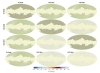 |
Fig. A.1 Frequency maps and difference maps using the GAL060 mask. Rms values are given in Table 1; histograms are shown in Fig. 4. In the top 3 × 3 group, the frequency maps are on the diagonal. The three frequency difference maps are in the upper right block. The noise difference maps are in the lower left block. The bottom row gives the single-frequency noise maps. The caption of Fig. 4 describes characteristics of the histograms that can also be seen quite clearly in these maps. The three upper right maps are the same as the three in Fig. 3, but with structure on scales larger than 8° removed, as described in the text. |
Appendix B: Nominal beam calibration: definitions, approximations, and rescaling factors
In the Planck scanning strategy, for each pointing period, the spin axis
remains fixed and the output voltage sees a spin-synchronous modulation as the telescope
points at direction  along a scan circle. The output signal (in arbitrary units) measured by a given
Planck detector, either LFI or HFI, can be written as
along a scan circle. The output signal (in arbitrary units) measured by a given
Planck detector, either LFI or HFI, can be written as  + M(\phat), \label{eq:Vout} \end{equation}](/articles/aa/full_html/2014/11/aa23743-14/aa23743-14-eq142.png) (B.1)where P is the angular response
(“beam”), normalized to unit solid angle (∫4πP dΩ =
1), D is the dipole signal (including the solar and
orbital terms), Tsky is the sky brightness temperature
(CMB and foregrounds, i.e., everything other than the dipole), and
M is a
small monopole term assumed to be constant for each pointing period
(B.1)where P is the angular response
(“beam”), normalized to unit solid angle (∫4πP dΩ =
1), D is the dipole signal (including the solar and
orbital terms), Tsky is the sky brightness temperature
(CMB and foregrounds, i.e., everything other than the dipole), and
M is a
small monopole term assumed to be constant for each pointing period
 .
We use the convolution notation A ∗ P =
∫4πAP dΩ.
.
We use the convolution notation A ∗ P =
∫4πAP dΩ.
For each pointing period, the output voltage measures a spin-synchronous modulation
dominated by the dipole, which is used to recover a gain calibration factor. The dipole
term, P ∗
D, is dominant (by two orders of magnitude) once
strong foreground regions are masked, so for calibration purposes we have Vout =
G(P ∗ D). For each
pointing period, calibration is performed by fitting Vout to a model
of the beam-convolved dipole: 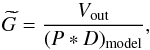 (B.2)where
  is the estimated gain, while
G =
Vout/ (P ∗
D) is the true gain. For the 2013 release, we rely on
the a priori knowledge of the solar dipole from WMAP (Hinshaw et al. 2009). Relative changes of the gain
is the estimated gain, while
G =
Vout/ (P ∗
D) is the true gain. For the 2013 release, we rely on
the a priori knowledge of the solar dipole from WMAP (Hinshaw et al. 2009). Relative changes of the gain
 between sky circles contribute to the monopole term
 ,
and are removed by destriping. Assuming an error-free knowledge of the true dipole and of
the full beam pattern, then Vout = (P ∗
D)model and
,
and are removed by destriping. Assuming an error-free knowledge of the true dipole and of
the full beam pattern, then Vout = (P ∗
D)model and
 , so one would recover the true value of
the gain, preserving the entire power entering the beam. However, full beam convolution
was not implemented in the LFI and HFI pipelines for the 2013 release, and we adopted a
“nominal beam approximation” approach.
, so one would recover the true value of
the gain, preserving the entire power entering the beam. However, full beam convolution
was not implemented in the LFI and HFI pipelines for the 2013 release, and we adopted a
“nominal beam approximation” approach.
Appendix B.1: Nominal beam approximation
We approximate the beam pattern with a “pencil beam”, i.e., a normalized
delta-function: 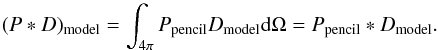 (B.3)Neglecting intrinsic errors in the model
dipole (Dmodel ≈
D), the estimated gain is
(B.3)Neglecting intrinsic errors in the model
dipole (Dmodel ≈
D), the estimated gain is
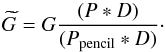 (B.4)We can write P as the sum of two
terms, P =
Pnominal +
Pside, where Pnominal
represents the contribution of the nominal beam (defined as the portion of the beam
defining the window function, see Sect. 4) and
Pside is the contribution from the (near
and far) sidelobes. We have
(B.4)We can write P as the sum of two
terms, P =
Pnominal +
Pside, where Pnominal
represents the contribution of the nominal beam (defined as the portion of the beam
defining the window function, see Sect. 4) and
Pside is the contribution from the (near
and far) sidelobes. We have 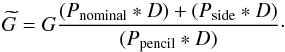 (B.5)The convolution of the nominal beam to the
dipole is nearly identical to an ideal pencil beam convolution, except that only a
fraction (1 −
fsl) of the antenna gain is contained in
the nominal beam, so we have
(B.5)The convolution of the nominal beam to the
dipole is nearly identical to an ideal pencil beam convolution, except that only a
fraction (1 −
fsl) of the antenna gain is contained in
the nominal beam, so we have  (B.6)where fsl is the
solid angle fraction of the sidelobes. For the 70, 100, and 143 GHz channels,
fsl ≈
0.7, 0.5, and 0.5% (see Sect. 4.1). In this formalism, we assume that the time response of the bolometers
has been accurately deconvolved; thus no additional time constant corrections are
needed. This approximation is true to high accuracy (<0.2%), since the dipole changes very
little within the nominal beam solid angle. Rearranging the terms, we find
(B.6)where fsl is the
solid angle fraction of the sidelobes. For the 70, 100, and 143 GHz channels,
fsl ≈
0.7, 0.5, and 0.5% (see Sect. 4.1). In this formalism, we assume that the time response of the bolometers
has been accurately deconvolved; thus no additional time constant corrections are
needed. This approximation is true to high accuracy (<0.2%), since the dipole changes very
little within the nominal beam solid angle. Rearranging the terms, we find 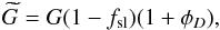 (B.7)where φD ≡
(Pside ∗
D)/(Pnominal ∗
D) represents the coupling of the dipole with
sidelobes and depends on the detailed structure of the sidelobes and the scanning
strategy. Equation (B.7) gives the
correction factor that one should apply to recover the proper gain factor if one models
the beam as a pencil beam.
(B.7)where φD ≡
(Pside ∗
D)/(Pnominal ∗
D) represents the coupling of the dipole with
sidelobes and depends on the detailed structure of the sidelobes and the scanning
strategy. Equation (B.7) gives the
correction factor that one should apply to recover the proper gain factor if one models
the beam as a pencil beam.
Appendix B.2: Rescaling factor
To obtain the reconstructed sky signal after calibration,
(),
the dipole term needs to be subtracted from the timelines (Eq. (B.1)). Since we are interested in the signal
from the sky entering the nominal beam, the coupling of Tsky with
sidelobes represents a spurious additive signal. So we write the timeline as
 (B.8)In the ideal case of an error-free,
full-convolution model, , one gets
(B.8)In the ideal case of an error-free,
full-convolution model, , one gets 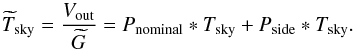 (B.9)For angular scales larger than the nominal
beam, a relation similar to Eq. (B.6)
holds for Tsky, i.e., Pnominal ∗
Tsky ≈ (1 −
fsl)Tsky.
With this and Eq. (B.9), we obtain
(B.9)For angular scales larger than the nominal
beam, a relation similar to Eq. (B.6)
holds for Tsky, i.e., Pnominal ∗
Tsky ≈ (1 −
fsl)Tsky.
With this and Eq. (B.9), we obtain
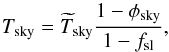 (B.10)where
 represents the coupling of the sidelobes
with the sky signal (other than the dipole), i.e., the straylight pickup.
represents the coupling of the sidelobes
with the sky signal (other than the dipole), i.e., the straylight pickup.
As mentioned, however, in the 2013 release both LFI and HFI used the nominal beam
approximation. In this case, the estimated gain is given by Eq. (B.7), and we have
 (B.11)Solving for the true sky temperature we
find
(B.11)Solving for the true sky temperature we
find ![Mathematical equation: \appendix \setcounter{section}{2} \begin{equation} \Tsky = \Tskyest \left[ 1 - {\phisky \over (1-\fsl)} + \phiD\right] \approx \Tskyest \left(1 - \phisky + \phiD\right). \label{eq:Tsky_corr--appendix} \end{equation}](/articles/aa/full_html/2014/11/aa23743-14/aa23743-14-eq179.png) (B.12)This expression does not contain the term
fsl to first order; however, the
(smaller) correction terms φD and
φsky need to be evaluated to derive the
proper normalization of the temperature maps and of the power spectra.
(B.12)This expression does not contain the term
fsl to first order; however, the
(smaller) correction terms φD and
φsky need to be evaluated to derive the
proper normalization of the temperature maps and of the power spectra.
In summary, to evaluate the true sky temperature from the estimated one, some correction factors need to be evaluated to properly account for the beam. These correction terms depend on the model assumptions. For a full convolution model, the rescaling factor is η = (1 − φsky)(1 − fsl). For a pencil beam approximation, currently applied by both Planck instruments, the rescaling factor is η = (1 − φsky + φD).
If one were to apply a correction, a rescaling factor η could be directly applied to the temperature map to give a properly calibrated map. Alternatively, the window function should be rescaled by η-2.
Appendix B.3: Semi-analytical expression for φD
A useful expression for φD can be obtained
as follows. The dipole seen through any particular line of sight (LOS) will be
proportional to the dot product of the dipole vector with that of the line of sight:
![Mathematical equation: \appendix \setcounter{section}{2} \begin{equation} D = D_0\left[ \sin \Theta_\mathrm{LOS}\cos\left(\Phi_\mathrm{LOS}-\Phi_{D}\right) + \cos \Theta_{D}\sin \Theta_\mathrm{LOS} \right], \label{eq:fullDipole} \end{equation}](/articles/aa/full_html/2014/11/aa23743-14/aa23743-14-eq186.png) (B.13)where D0 = 3.35 mK,
the amplitude of the dipole, ΘD and ΦD are the
polar and azimuthal angles of the direction of the dipole maximum on the sky9, and ΘLOS and ΦLOS are the same for the direction of the nominal beam
observation. For each ring, choosing a coordinate system for which the z-axis is aligned with
the satellite spin axis, and around which both the LOS and the dipole axis will rotate,
ensures that the last term in Eq. (B.13)
is constant. Since a constant is removed for each stable pointing period (Planck Collaboration VIII 2014), we ignore this and
write
(B.13)where D0 = 3.35 mK,
the amplitude of the dipole, ΘD and ΦD are the
polar and azimuthal angles of the direction of the dipole maximum on the sky9, and ΘLOS and ΦLOS are the same for the direction of the nominal beam
observation. For each ring, choosing a coordinate system for which the z-axis is aligned with
the satellite spin axis, and around which both the LOS and the dipole axis will rotate,
ensures that the last term in Eq. (B.13)
is constant. Since a constant is removed for each stable pointing period (Planck Collaboration VIII 2014), we ignore this and
write  (B.14)Specializing, when the line of sight (LOS)
is the nominal beam, the signal seen will be
(B.14)Specializing, when the line of sight (LOS)
is the nominal beam, the signal seen will be  (B.15)Similarly, when we observe a point on the
sky through a sidelobe, we have
(B.15)Similarly, when we observe a point on the
sky through a sidelobe, we have  (B.16)where ΔΦsl = Φsl −
Φmain is the difference in azimuthal angles between the
nominal beam and the sidelobe of interest. This yields:
(B.16)where ΔΦsl = Φsl −
Φmain is the difference in azimuthal angles between the
nominal beam and the sidelobe of interest. This yields:  (B.17)Because Planck calibrates
by “locking in” on, or fitting to, a sinusoidal signal of the form
(B.17)Because Planck calibrates
by “locking in” on, or fitting to, a sinusoidal signal of the form
 (Eq. (B.15)), the second term in Eq. (B.17) is irrelevant, and the far sidelobes will make a contribution
to the gain according to
(Eq. (B.15)), the second term in Eq. (B.17) is irrelevant, and the far sidelobes will make a contribution
to the gain according to  (B.18)Integrations over GRASP models of the HFI
far sidelobes indicate that φD ≈ fFSL/
3.
(B.18)Integrations over GRASP models of the HFI
far sidelobes indicate that φD ≈ fFSL/
3.
Appendix C: Assessment of LFI and HFI with respect to beams and calibration
Appendix C.1: LFI
Appendix C.1.1: Evaluation of φsky
The term φsky turns out to be small, but it is difficult to quantify because it requires a full convolution of a sky model with the full beam, and it is frequency dependent. We have performed a simplified simulation for a 70 GHz channel (LFI18M), and find values for φsky ranging between 0.05% and 0.2% throughout a full survey. More realistic simulations have been produced recently on an LFI 30 GHz channel (LFI27M), for both Survey 1 and Survey 2. We find:
Survey 1, ⟨ φsky ⟩ = 0.05%, 0.01% <φsky< 0.23%;
Survey 2, ⟨ φsky ⟩ = 0.06%, 0.01% <φsky< 1.11%.
(Differences between odd and even Surveys are to be expected, given the differences in scanning described in Planck Collaboration I 2014, Sect. 4.1.) These results are consistent with our preliminary findings, and indicate a typical value of φsky ≈ 0.05% at all Planck frequencies.
Appendix C.1.2: Evaluation of φD
We can estimate φD by taking average values of the convolutions involved in its definition in Eq. (B.12). The denominator ⟨ Pnominal ∗ D ⟩ = 3.35 mK is the dipole amplitude. To estimate ⟨ Pside ∗ D ⟩, we have computed the convolution of the LFI sidelobes, modelled with GRASP, with the dipole.
Note that φD contains the effects of both near and far sidelobes; however, it is the dipole modulation through the near sidelobes that contributes most to its value. Destriping removes the contribution from sidelobes nearly aligned with the spacecraft spin axis (such as the “primary spillover,” see Planck Collaboration I 2014), which produces a nearly constant offset for each pointing period. After destriping, we find that ⟨ Pside ∗ D ⟩ is approximately 3 μK at 70 GHz and 5 μK at 30 GHz, leading to ⟨ φD ⟩ ≈ 0.1% and ⟨ φD ⟩ ≈ 0.15%, respectively.
Figure C.1 shows the pixel histogram for a simulation where the value of φD was computed in every sky direction for an LFI 70 GHz channel. The median value, φD ≈ 0.16%, is in good agreement with our first-order estimate.
 |
Fig. C.1 φD for a simulation using a 70 GHz beam. |
In conclusion, the correction terms φD and φsky are of the same order (0.15% and 0.05%, respectively) and tend to cancel each other in Eq. (B.12), resulting in a net effect of ≈0.1% on the LFI calibrated map. For the 2013 release, we have not carried out a systematic simulation for all channels; rather we have assumed a conservative residual uncertainty of 0.2% in the LFI calibrated maps due to sidelobe convolution effects (Planck Collaboration V 2014, Table 8). More detailed analysis is planned for the 2014 release.
Appendix C.2: HFI
The effective beam window function, including the effects of both calibration and map reconstruction, is based on measurements of the scanning beam (Planck Collaboration VII 2014). These are obtained from Mars observations after deconvolution of the time response of the detection chain. The effective beam window function is used to correct the cross-power spectra used in the cosmological analysis. Figure 10 of Planck Collaboration VII (2014) shows this scanning beam, and provides estimates of the near sidelobe contribution to the solid angle between 0.1 and 0.2% at 100 and 143 GHz, respectively. In the subsections below, we estimate the impact of the approximations used in estimating the nominal beam and near sidelobe region (up to 5° from the beam centre) through the use of Saturn and Jupiter observations. We estimate the bias introduced by these approximations, as well as the bias in the calibration factor due to the far sidelobes. As previously stated, we make no attempt to recalibrate the 2013 data release, but only show that the LFI–HFI differences at intermediate multipoles are understood within the present uncertainties.
Appendix C.2.1: Nominal beam and near sidelobes
The nominal beam for HFI is measured to roughly 15′ with Mars observations. This provides most of the information needed for the high-ℓ analysis used to obtain the 2013 Planck cosmological results. Jupiter observations show shoulders extending to 20′ for all channels (see fogire 10 of Planck Collaboration VII 2014). Features in this region are small and difficult to measure. Their integrated contribution, however, is not negligible at the level of a few tenths of a percent. Table 2 and Fig. 10 of Planck Collaboration VII (2014) show estimates of the near sidelobe contribution to the solid angle of between 0.1 and 0.22%.
In addition, pre-launch optical calculations show that at a few FWHM from the beam centre, the HFI beam will have a diffraction pattern from the secondary mirror edges (the pupil of the Planck optical system). Figure 14 of Planck Collaboration VII (2014) shows that at 353 GHz there are near sidelobes with a diffraction signature, which have not been accounted for. These features are expected from optical calculations, and they were seen in the pre-launch test campaign. A reanalysis of Saturn and Jupiter data has been carried out for all frequencies, and the near sidelobe wing due to diffraction by the edge of the secondary is seen at least at 143 GHz and higher frequencies. Additionally, the sidelobe profiles of Planck Collaboration VII (2014) led to a removal of the residual time response effects with a weighting that also removed optical near sidelobe signal around 20′.
In order to assess the impact of a more refined accounting of the near sidelobes, we have constructed a new hybrid beam profile that consists of the nominal beam, azimuthally averaged Jupiter observations, and GRASP simulations. The azimuthally averaged Jupiter observations extend to 2°, and include all residual time response and mirror dimpling effects. The astrophysical background is subtracted from each observation, and we fit a baseline and a scaling factor to match the Jupiter profile to the Mars profile at an overlap angle. The GRASP simulations consist of all eight 100 GHz detectors simulated at five frequencies across the band. A 100 GHz full-frequency beam is constructed by weighting the simulations with the map-making weights, detector bandpass, and planet spectral energy distribution. At large angle, the GRASP calculations are dominated by diffraction around the secondary mirror. The diffraction pattern has a similar angular dependence at all HFI frequencies, and its normalization is set by the edge taper of the secondary. We therefore scale the 100 GHz simulations to higher frequencies by fitting to the Jupiter profile. Figure C.2 shows the radial profiles of the hybrid beams, compared with those given in Planck Collaboration VII (2014).
The Saturn-Jupiter combination (Fig. C.2) gives a diffraction pattern similar to that predicted and measured preflight (Tauber et al. 2010). This increases the estimate of the contribution of the near sidelobes to the total solid angle of beam, as given in Fig. 10 of Planck Collaboration VII (2014). However, the dominant contribution to the increase in solid angle at 100 and 143 GHz occurs around 20′, and is due to removing the assumption of azimuthal symmetry and applying no time response correction when computing the radial profile.
 |
Fig. C.2 HFI beam and planet measurement profiles. The grey shaded region shows the 1σ errors in the nominal beam profile used to make the effective beam window function. The dashed blue and red lines are the best-case and worst-case near sidelobe estimates from Jupiter, presented in Fig. 10 of Planck Collaboration VII (2014). The solid green curve is the hybrid beam profile used to derive correction factors here. The vertical dotted lines indicate the radial extent of each portion of the hybrid beam: the nominal beam is at small angles; at intermediate angles Jupiter data are used; and at large angles the scaled GRASP simulation is used. |
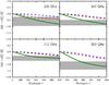 |
Fig. C.3 Effective beam window function corrections based on the hybrid beam profile. The green curve shows the correction based on the hybrid model presented here. The dashed blue and red lines are the best-case and worst-case near sidelobe estimates from Jupiter, as shown in Fig. 10 of Planck Collaboration VII (2014). The grey shaded region shows the ±1σ errors in the correction to the solid angle. |
This also affects the shape of the effective beam window function, with a decrease similar to that illustrated in the green curve in Fig. 19 of Planck Collaboration VII (2014), although with a larger amplitude and large error bars (Fig. C.3). The effect of these corrections for near-sidelobe power missing in the beams used in the 2013 results is illustrated in Fig. 12. The error in the integral of the beam profile is dominated by the background removal and inter-calibration of the Mars and Jupiter data.
Appendix C.2.2: Far sidelobes
Estimates from Tauber et al. (2010) put the integrated solid angle of the far sidelobes at roughly 0.3% of the total beam solid angle. While this is small, a significant fraction of this solid angle appears near the satellite spin axis. This means that the signal seen through this part of the sidelobes is not modulated by the satellite rotation, and therefore does not contribute to the calibration. Using calculations such as those in Sect. C.1.2, we estimate the far sidelobe effect on the calibration to be of order one-third the total solid angle for the far sidelobes. For HFI, this constitutes about 0.1% at 100 and 143 GHz.
All Tables
Summary of ratios of Planck 70, 100, and 143 GHz power spectra appearing in this paper.
Summary of ratios of Planck 70 and 100 GHz and WMAP V- and W-band power spectra appearing in this paper.
All Figures
|
Fig. 1 Sky masks used for spectral analysis of the Planck 70, 100, and 143 GHz maps. The light blue, yellow, and red masks leave observable sky fractions fsky of 39.7%, 59.6%, and 69.4%, respectively, and are named GAL040, GAL060, and GAL070 in the PLA. These masks are extended by exclusion of unresolved sources in the PCCS 70, 100, and 143 GHz source lists above the 5σ flux density cuts. |
| In the text | |
|
Fig. 2 Sky maps used in the analysis of Planck data consistency. Top row: 70 GHz. Middle row: 100 GHz. Bottom row: 143 GHz. Left column: signal maps. Right column: noise maps derived from half-ring differences. All maps are Nside = 2048. These are the publicly-released maps corrected for monopole and dipole terms as described in the text. The impression of overall colour differences between the maps is due to the interaction between noise, the colour scale, and display resolution. For example, the larger positive and negative swings between pixels in the 70 GHz noise map pick up darker reds and blues farther from zero. Smaller swings around zero in the 100 and 143 GHz noise maps result in pastel yellows and blues in adjacent pixels, which when displayed at less than full-pixel resolution give an overall impression of green, a colour not used in the colour bar. |
| In the text | |
|
Fig. 3 Difference maps. Top: 100 GHz minus 70 GHz. Middle: 143 GHz minus 100 GHz. Bottom: 143 GHz minus 70 GHz. All sky maps are smoothed to angular resolution FWHM = 15′ by a filter that accounts for the difference between the effective beam response at each frequency and a Gaussian of FWHM 15′. These maps illustrate clearly the difference in the noise level of the individual maps, excellent overall nulling of the CMB anisotropy signal, and frequency-dependent foregrounds. The 100–70 difference shows predominantly CO (J = 0 → 1) emission (positive) and free-free emission (negative). The 143–100 difference shows dust emission (positive) and CO emission (negative). The 143–70 difference shows dust emission (positive) and free-free emission (negative). The darker stripe in the top and bottom maps is due to reduced integration time in the 70 GHz channel in the first days of observation (see Planck Collaboration II 2014, Sect. 9.5). |
| In the text | |
|
Fig. 4 Signal and noise for the frequency maps of Fig. 2 (left panel) and the difference maps of Fig. 3 (right panel), with the 59.6% mask in all cases. The broader, signal+noise curves are nearly Gaussian due to the dominant CMB anisotropies. The 70 GHz curve is broader than the 100 and 143 GHz curves because of the higher noise level, but is still signal-dominated for | dT/T | ≳ 50 μK. The narrower noise curves, derived from the half-ring difference maps, are not Gaussian because of the scanning-induced spatial dependence of pixel noise in Planck maps. The considerably higher noise level of the 70 GHz map is again apparent. The histograms of the difference maps show noise domination near the peak of each pair of curves (the signal+noise and noise curves overlap). The pairs involving 70 GHz are wider and dominated by the 70 GHz noise, but the wings at low pixel counts show the signature of foregrounds that exceed the noise levels, primarily dust and CO emission in the negative wing, and free-free and synchrotron emission in the positive wing. In the low-noise 100 minus 143 GHz pairs, the signal, due mostly to dust emission in the negative wing and to free-free and CO residuals in the positive wing, stands out clearly from the noise. |
| In the text | |
|
Fig. 5 Planck 70, 100, and 143 GHz CMB anisotropy power spectra computed
for the GAL060 mask. Mask- and beam-deconvolved cross-spectra of the half-ring maps
show the signal; auto-correlation spectra of the half-ring difference maps show the
noise. Points show single multipoles up to ℓ = 1200 for 70 GHz
and ℓ =
1700 for 100 and 143 GHz. Heavy solid lines show Δℓ = 20 boxcar
averages. The S/N near the first peak (ℓ = 220) is approximately 80, 1900, and 6000
for 70, 100, and 143 GHz, respectively. Noise power is calculated according to the
large-ℓ approximation, i.e., as a
|
| In the text | |
|
Fig. 6 Spectral analysis of the Planck 70, 100, and 143 GHz maps. Columns show results computed using the three sky masks in Fig. 1, with, from left to right, fsky = 69.4%, 59.6%, and 39.7%. Top row: CMB anisotropy spectra binned over a range of multipoles Δℓ = 40, for ℓ ≥ 30, with (2ℓ + 1)-weighting applied within the bin. Error bars are computed as a measure of the rms-power within each bin, and hence comprise both the measurement inaccuracy and cosmic variance. The grey curve is the best-fit Planck 6-parameter ΛCDM model from Planck Collaboration XVI (2014). Noise spectra computed from the half-ring-difference maps are shown: for the 70 GHz channel, the S/N ≈ 1 at ℓ ≈ 650. Middle row: residuals of the same power spectra with respect to the Planck best-fit model. Bottom row: power ratios for the 70 vs. 100 GHz and 143 vs. 100 GHz channels of Planck. The ratios are calculated ℓ by ℓ, then binned. The error bars show the standard error of the mean for the bin. The effect of diffuse foregrounds is clearly seen in the changes in the 143/100 ratio with sky fraction at ℓ ≈ 100. Bin-to-bin variations in the exact values of the ratios with sky fraction emphasize the importance of making such comparisons precisely. |
| In the text | |
|
Fig. 7 Same as the top two panels of the middle column of Fig. 6, but without inclusion of signal cosmic variance in the uncertainties. Both signal × noise and noise × noise terms are included. |
| In the text | |
|
Fig. 8 Estimates of the residual thermal SZ and unresolved radio and infrared source residuals that must be removed. |
| In the text | |
|
Fig. 9 Same as the bottom middle panel of Fig. 6, but corrected for differences in unresolved-source residuals (see text). We have not tried to account for uncertainties in the foreground correction itself; however, since the correction is small, the effect on the uncertainties would be small. |
| In the text | |
|
Fig. 10 Radial slice through a 70 GHz beam from the GRASP model, illustrating the nominal beam, near sidelobe, and far sidelobe regions. The exact choice of angular cutoff for the nominal beam is different for different frequencies. |
| In the text | |
|
Fig. 11 Effective beam window function corrections from Fig. C.3, which correct for the effect of near-sidelobe power missing in the HFI beams used in the 2013 results (Sect. C.2.1). Uncertainties are not shown here for clarity, but are shown in Fig. C.3, and would be large on the scale of this plot. The 217 GHz correction is shown for illustration only. |
| In the text | |
|
Fig. 12 Same as the bottom middle panel of Fig. 6, but corrected for the near-sidelobe power at 100 and 143 GHz that was not included in the 2013 results. Since the beam corrections for 100 and 143 GHz are nearly identical, the ratio 143/100 hardly changes. The ratio 70/100, however, changes significantly, moving towards unity. Uncertainties in the beam window function corrections are not included. |
| In the text | |
|
Fig. 13 Same as the bottom middle panel of Fig. 6, but corrected for both the near-sidelobe power at 100 and 143 GHz that was not included in the 2013 results and for unresolved source residuals (Sect. 3.3). Uncertainties in the beam window function corrections are not included. |
| In the text | |
|
Fig. 14 Ratios of 100, 143, and 217 GHz power spectra calculated from detector sets with the likelihood method, including subtraction of the best-fitting foreground model (see text) and correction for the best-fit relative calibration factors for individual detectors. Solid symbols and lines show ratios for mask G22; open symbols and dotted or dashed lines show ratios for mask G35. The greater scatter in 217/143 for mask G35 is caused by CMB-foreground cross-correlations. |
| In the text | |
|
Fig. 15 Effects on the 143/100 ratio of changes in the mask, choice of detectors, and detector recalibration. Solid lines indicate ratios calculated with mask G22; dashed lines indicate mask G35. Use of detector sets gives the cyan curves with recalibration turned on and the red curves with recalibration turned off. Use of full-frequency half-ring cross spectra, as in Sect. 3, gives the blue curves. The cyan curves are comparable to the green curves in Fig. 14, which also have intra-frequency calibration and foreground corrections applied. The blue-dashed curve agrees extremely well with the blue curve in the bottom right panel of Fig. 6, as it should (see text). |
| In the text | |
|
Fig. 16 Changes in cosmological parameters from the inclusion of the near sidelobe power discussed in the text. The black curves are the 2013 results for Planck plus the low-ℓ WMAP polarization (WP). The red curves are for Planck+WP using the revised HFI beams. The shifts in the posteriors are all less than 0.3σ except for the cosmological amplitude As and parameters related to it, as expected. |
| In the text | |
|
Fig. 17 Changes in the beam eigenmode coefficients from the inclusion of the near-sidelobe power now established but not included in the processing for the 2013 results. Black curves are for Planck+WP; red curves are for Planck+WP with the revised beams. The superscript indicates the effective spectum (one to four for 100, 143, 217, and 143 × 217 respectively) while the subscript indicates eigenmode number. |
| In the text | |
|
Fig. 18 Planckfsky ≈ 60% Galactic mask in yellow and WMAP KQ75 at Nside = 1024 in red. The mask used for comparative spectral analysis of the Planck 70, 100, and 143 GHz, and WMAP nine-year V- and W-band sky maps is the union of the two. The joint Planck 70, 100, and 143 GHz point source mask is also used, exactly as before. The final sky fraction is fsky = 56.7%. The Planck mask is degraded to the pixel resolution Nside = 1024, at which the yearly WMAP individual differential assembly maps are available. |
| In the text | |
|
Fig. 19 Left: WMAP V band compared to Planck 70 GHz and best-fit model. Right: WMAP W band compared to Planck 100 GHz and best-fit model. The joint Planck/KQ75 sky mask + Planck point source mask (fsky = 56.7%; see Fig. 18) is used. Because the frequencies are so close, no corrections for foregrounds are made. |
| In the text | |
|
Fig. 20 Ratios of power spectra for Planck and WMAP over the joint Planck/KQ75+Planck point source mask with fsky = 56.7%. The Planck 70/100 and 143/100 ratios can be compared to the bottom middle panel in Fig. 6 for fsky = 59.6%. Here we limit the horizontal scale because the WMAP noise beyond ℓ = 400 makes the ratios uninformative. The general shape of the Planck ratios is the same; however, it is clear (as it was in Fig. 6) that changes in the sky fraction change the ratios significantly within the uncertainties. This underscores the importance of strict equality of all factors in such comparisons. |
| In the text | |
|
Fig. 21 Same as Fig. 20, but the Planck 70/100 and 143/100 ratios are corrected for beam power at 100 and 143 GHz that was not included in the effective beam window function used in the 2013 results. |
| In the text | |
|
Fig. 22 Same as Fig. 20, but including corrections for both Planck beams and for Planck and WMAP unresolved-source residuals. |
| In the text | |
|
Fig. 23 Foreground-corrected spectra computed using mask G56, with calibration factors cX from Eq. (3) applied to 70 GHz, V, W, and V + W. The solid red lines in the upper panels show the best-fit model CMB spectrum (Planck Collaboration XVI 2014). The lower panels show the residuals with respect to this model. The error bars on the LFI and WMAP points show noise errors only. |
| In the text | |
|
Fig. A.1 Frequency maps and difference maps using the GAL060 mask. Rms values are given in Table 1; histograms are shown in Fig. 4. In the top 3 × 3 group, the frequency maps are on the diagonal. The three frequency difference maps are in the upper right block. The noise difference maps are in the lower left block. The bottom row gives the single-frequency noise maps. The caption of Fig. 4 describes characteristics of the histograms that can also be seen quite clearly in these maps. The three upper right maps are the same as the three in Fig. 3, but with structure on scales larger than 8° removed, as described in the text. |
| In the text | |
|
Fig. C.1 φD for a simulation using a 70 GHz beam. |
| In the text | |
|
Fig. C.2 HFI beam and planet measurement profiles. The grey shaded region shows the 1σ errors in the nominal beam profile used to make the effective beam window function. The dashed blue and red lines are the best-case and worst-case near sidelobe estimates from Jupiter, presented in Fig. 10 of Planck Collaboration VII (2014). The solid green curve is the hybrid beam profile used to derive correction factors here. The vertical dotted lines indicate the radial extent of each portion of the hybrid beam: the nominal beam is at small angles; at intermediate angles Jupiter data are used; and at large angles the scaled GRASP simulation is used. |
| In the text | |
|
Fig. C.3 Effective beam window function corrections based on the hybrid beam profile. The green curve shows the correction based on the hybrid model presented here. The dashed blue and red lines are the best-case and worst-case near sidelobe estimates from Jupiter, as shown in Fig. 10 of Planck Collaboration VII (2014). The grey shaded region shows the ±1σ errors in the correction to the solid angle. |
| In the text | |
Current usage metrics show cumulative count of Article Views (full-text article views including HTML views, PDF and ePub downloads, according to the available data) and Abstracts Views on Vision4Press platform.
Data correspond to usage on the plateform after 2015. The current usage metrics is available 48-96 hours after online publication and is updated daily on week days.
Initial download of the metrics may take a while.