| Issue |
A&A
Volume 571, November 2014
Planck 2013 results
|
|
|---|---|---|
| Article Number | A7 | |
| Number of page(s) | 31 | |
| Section | Astronomical instrumentation | |
| DOI | https://doi.org/10.1051/0004-6361/201321535 | |
| Published online | 29 October 2014 | |
Planck 2013 results. VII. HFI time response and beams
1
APC, AstroParticule et Cosmologie, Université Paris Diderot,
CNRS/IN2P3, CEA/lrfu, Observatoire de Paris, Sorbonne Paris Cité, 10 rue Alice Domon et Léonie
Duquet, 75205
Paris Cedex 13,
France
2
Aalto University Metsähovi Radio Observatory,
Metsähovintie 114, 02540
Kylmälä,
Finland
3
African Institute for Mathematical Sciences,
6-8 Melrose Road, 7954 Muizenberg,
Cape Town, South
Africa
4
Agenzia Spaziale Italiana Science Data Center,
via del Politecnico snc,
00133
Roma,
Italy
5
Agenzia Spaziale Italiana, Viale Liegi 26, 00198
Roma,
Italy
6
Astrophysics Group, Cavendish Laboratory, University of
Cambridge, J J Thomson
Avenue, Cambridge
CB3 0HE,
UK
7
Astrophysics & Cosmology Research Unit, School of Mathematics,
Statistics & Computer Science, University of KwaZulu-Natal,
Westville Campus,Private Bag
X54001, 4000
Durban, South
Africa
8
Atacama Large Millimeter/submillimeter Array, ALMA Santiago Central
Offices, Alonso de Cordova 3107,
Vitacura, Casilla
763 0355
Santiago
Chile
9
CITA, University of Toronto, 60 St. George St., Toronto, ON
M5S 3H8,
Canada
10
CNRS, IRAP, 9 Av.
colonel Roche, BP
44346, 31028
Toulouse Cedex 4,
France
11
California Institute of Technology, Pasadena, California, USA
12
Centre for Theoretical Cosmology, DAMTP, University of
Cambridge, Wilberforce
Road, Cambridge
CB3 0WA,
UK
13
Centro de Estudios de Física del Cosmos de Aragón
(CEFCA), Plaza San Juan, 1, planta
2, 44001
Teruel,
Spain
14
Computational Cosmology Center, Lawrence Berkeley National
Laboratory, Berkeley,
California,
USA
15
DSM/Irfu/SPP, CEA-Saclay, 91191
Gif-sur-Yvette Cedex,
France
16
DTU Space, National Space Institute, Technical University of
Denmark, Elektrovej
327, 2800
Kgs. Lyngby,
Denmark
17
Département de Physique Théorique, Université de
Genève, 24 quai E.
Ansermet, 1211
Genève 4,
Switzerland
18
Departamento de Física Fundamental, Facultad de Ciencias,
Universidad de Salamanca, 37008
Salamanca,
Spain
19
Department of Astronomy and Astrophysics, University of
Toronto, 50 Saint George Street,
Toronto, Ontario,
Canada
20
Department of Astrophysics/IMAPP, Radboud University
Nijmegen, PO Box
9010, 6500 GL
Nijmegen, The
Netherlands
21
Department of Electrical Engineering and Computer Sciences,
University of California, Berkeley, California, USA
22
Department of Physics & Astronomy, University of British
Columbia, 6224 Agricultural Road,
Vancouver, British
Columbia, Canada
23
Department of Physics and Astronomy, Dana and David Dornsife College
of Letter, Arts and Sciences, University of Southern California,
Los Angeles, CA
90089,
USA
24
Department of Physics and Astronomy, University College
London, London
WC1E 6BT,
UK
25
Department of Physics, Florida State University, Keen Physics
Building, 77 Chieftan
Way, Tallahassee,
Florida,
USA
26
Department of Physics, Gustaf Hällströmin katu 2a, University of
Helsinki, 00014
Helsinki,
Finland
27
Department of Physics, Princeton University,
Princeton, New Jersey, USA
28
Department of Physics, University of California,
One Shields Avenue, Davis, California, USA
29
Department of Physics, University of California,
Santa Barbara, California, USA
30
Department of Physics, University of Illinois at
Urbana-Champaign, 1110 West Green
Street, Urbana,
Illinois,
USA
31
Dipartimento di Fisica e Astronomia G. Galilei, Università degli
Studi di Padova, via Marzolo
8, 35131
Padova,
Italy
32
Dipartimento di Fisica e Scienze della Terra, Università di
Ferrara, via Saragat
1, 44122
Ferrara,
Italy
33
Dipartimento di Fisica, Università La Sapienza,
P. le A. Moro 2, 00185
Roma,
Italy
34
Dipartimento di Fisica, Università degli Studi di
Milano, via Celoria,
16, 20133
Milano,
Italy
35
Dipartimento di Fisica, Università degli Studi di
Trieste, via A. Valerio
2, 34127
Trieste,
Italy
36
Dipartimento di Fisica, Università di Roma Tor
Vergata, via della Ricerca Scientifica,
1, 00133
Roma,
Italy
37
Discovery Center, Niels Bohr Institute, Blegdamsvej 17, 2100
Copenhagen,
Denmark
38
European Southern Observatory, ESO Vitacura, Alonso de Cordova 3107, Vitacura,
Casilla
19001
Santiago,
Chile
39
European Space Agency, ESAC, Planck Science Office, Camino bajo del
Castillo, s/n, Urbanización
Villafranca del Castillo, 28692 Villanueva de la Cañada, Madrid, Spain
40
European Space Agency, ESTEC, Keplerlaan 1, 2201 AZ
Noordwijk, The
Netherlands
41
Helsinki Institute of Physics, Gustaf Hällströmin katu 2, University of Helsinki,
00014
Helsinki,
Finland
42
INAF – Osservatorio Astrofisico di Catania,
via S. Sofia 78, 95123
Catania,
Italy
43
INAF – Osservatorio Astronomico di Padova,
Vicolo dell’Osservatorio 5,
35122
Padova,
Italy
44
INAF – Osservatorio Astronomico di Roma,
via di Frascati 33, 00040
Monte Porzio Catone,
Italy
45
INAF – Osservatorio Astronomico di Trieste,
via G.B. Tiepolo 11, 34143
Trieste,
Italy
46
INAF Istituto di Radioastronomia, via P. Gobetti 101, 40129
Bologna,
Italy
47
INAF/IASF Bologna, via Gobetti 101, 40129
Bologna,
Italy
48
INAF/IASF Milano, via E. Bassini 15, 20133
Milano,
Italy
49
INFN, Sezione di Bologna, via Irnerio 46, 40126
Bologna,
Italy
50
INFN, Sezione di Roma 1, Università di Roma Sapienza,
Piazzale Aldo Moro 2,
00185
Roma,
Italy
51
IPAG:Institut de Planétologie et d’Astrophysique de Grenoble,
Université Joseph Fourier, Grenoble 1/CNRS-INSU, UMR 5274, 38041
Grenoble,
France
52
IUCAA, Post Bag 4, Ganeshkhind, Pune University
Campus, 411 007
Pune,
India
53
Imperial College London, Astrophysics group, Blackett
Laboratory, Prince Consort
Road, London,
SW7 2AZ,
UK
54
Infrared Processing and Analysis Center, California Institute of
Technology, Pasadena,
CA
91125,
USA
55
Institut Néel, CNRS, Université Joseph Fourier Grenoble
I, 25 rue des
Martyrs, 38042
Grenoble,
France
56
Institut Universitaire de France, 103 bd Saint-Michel, 75005, Paris, France
57
Institut d’Astrophysique Spatiale, CNRS (UMR 8617) Université
Paris-Sud 11, Bâtiment
121, 91405
Orsay,
France
58
Institut d’Astrophysique de Paris, CNRS (UMR 7095),
98bis boulevard Arago,
75014
Paris,
France
59
Institute for Space Sciences, 077125
Bucharest-Magurale,
Romania
60
Institute of Astronomy and Astrophysics, Academia
Sinica, 10617
Taipei,
Taiwan
61
Institute of Astronomy, University of Cambridge,
Madingley Road, Cambridge
CB3 0HA,
UK
62
Institute of Theoretical Astrophysics, University of
Oslo, Blindern,
0315
Oslo,
Norway
63
Instituto de Física de Cantabria (CSIC-Universidad de
Cantabria), Avda. de los Castros
s/n, 39005
Santander,
Spain
64
Jet Propulsion Laboratory, California Institute of
Technology, 4800 Oak Grove
Drive, Pasadena,
California,
USA
65
Jodrell Bank Centre for Astrophysics, Alan Turing Building, School
of Physics and Astronomy, The University of Manchester, Oxford Road, Manchester, M13
9PL, UK
66
Kavli Institute for Cosmology Cambridge,
Madingley Road, Cambridge, CB3 0HA, UK
67
LAL, Université Paris-Sud, CNRS/IN2P3, 91898
Orsay,
France
68
LERMA, CNRS, Observatoire de Paris, 61 avenue de l’Observatoire, 75014
Paris,
France
69
Laboratoire AIM, IRFU/Service d’Astrophysique – CEA/DSM – CNRS –
Université Paris Diderot, Bât. 709,
CEA-Saclay, 91191
Gif-sur-Yvette Cedex,
France
70
Laboratoire Traitement et Communication de l’Information, CNRS (UMR
5141) and Télécom ParisTech, 46 rue
Barrault, 75634
Paris Cedex 13,
France
71
Laboratoire de Physique Subatomique et de Cosmologie, Université
Joseph Fourier Grenoble I, CNRS/IN2P3, Institut National Polytechnique de
Grenoble, 53 rue des
Martyrs, 38026
Grenoble Cedex,
France
72
Laboratoire de Physique Théorique, Université Paris-Sud 11 &
CNRS, Bâtiment 210,
91405
Orsay,
France
73
Lawrence Berkeley National Laboratory, Berkeley, California, USA
74
Max-Planck-Institut für Astrophysik, Karl-Schwarzschild-Str. 1, 85741
Garching,
Germany
75
McGill Physics, Ernest Rutherford Physics Building, McGill
University, 3600 rue
University, Montréal,
QC, H3A 2T8, Canada
76
National University of Ireland, Department of Experimental
Physics, Maynooth,
Co. Kildare,
Ireland
77
Niels Bohr Institute, Blegdamsvej 17, Copenhagen, Denmark
78
Observational Cosmology, Mail Stop 367-17, California Institute of
Technology, Pasadena,
CA
91125,
USA
79
Optical Science Laboratory, University College London,
Gower Street, London, UK
80
SB-ITP-LPPC, EPFL, CH-1015
Lausanne,
Switzerland
81
SISSA, Astrophysics Sector, via Bonomea 265, 34136
Trieste,
Italy
82
School of Physics and Astronomy, Cardiff University,
Queens Buildings, The Parade,
Cardiff, CF24 3AA, UK
83
Space Sciences Laboratory, University of California,
Berkeley, California, USA
84
Special Astrophysical Observatory, Russian Academy of
Sciences, Nizhnij Arkhyz,
Zelenchukskiy region, 369167
Karachai-Cherkessian Republic,
Russia
85
Stanford University, Dept of Physics, Varian Physics Bldg, 382 via Pueblo
Mall, Stanford,
California,
USA
86
Sub-Department of Astrophysics, University of Oxford,
Keble Road, Oxford
OX1 3RH,
UK
87
Theory Division, PH-TH, CERN, 1211
Geneva 23,
Switzerland
88
UPMC Univ Paris 06, UMR7095, 98bis boulevard Arago, 75014
Paris,
France
89
Université de Toulouse, UPS-OMP, IRAP, 31028
Toulouse Cedex 4,
France
90
University of Granada, Departamento de Física Teórica y del Cosmos,
Facultad de Ciencias, 18071
Granada,
Spain
91
Warsaw University Observatory, Aleje Ujazdowskie 4, 00-478
Warszawa,
Poland
Received:
21
March
2013
Accepted:
10
December
2013
Abstract
This paper characterizes the effective beams, the effective beam window functions and the associated errors for the Planck High Frequency Instrument (HFI) detectors. The effective beam is theangular response including the effect of the optics, detectors, data processing and the scan strategy. The window function is the representation of this beam in the harmonic domain which is required to recover an unbiased measurement of the cosmic microwave background angular power spectrum. The HFI is a scanning instrument and its effective beams are the convolution of: a) the optical response of the telescope and feeds; b) the processing of the time-ordered data and deconvolution of the bolometric and electronic transfer function; and c) the merging of several surveys to produce maps. The time response transfer functions are measured using observations of Jupiter and Saturn and by minimizing survey difference residuals. The scanning beam is the post-deconvolution angular response of the instrument, and is characterized with observations of Mars. The main beam solid angles are determined to better than 0.5% at each HFI frequency band. Observations of Jupiter and Saturn limit near sidelobes (within 5°) to about 0.1% of the total solid angle. Time response residuals remain as long tails in the scanning beams, but contribute less than 0.1% of the total solid angle. The bias and uncertainty in the beam products are estimated using ensembles of simulated planet observations that include the impact of instrumental noise and known systematic effects. The correlation structure of these ensembles is well-described by five error eigenmodes that are sub-dominant to sample variance and instrumental noise in the harmonic domain. A suite of consistency tests provide confidence that the error model represents a sufficient description of the data. The total error in the effective beam window functions is below 1% at 100 GHz up to multipole ℓ ~ 1500, and below 0.5% at 143 and 217 GHz up to ℓ ~ 2000.
Key words: cosmic background radiation / cosmology: observations / instrumentation: detectors / surveys
Corresponding author: B. P. Crill, e-mail: This email address is being protected from spambots. You need JavaScript enabled to view it.
© ESO, 2014
1. Introduction
This paper, one of a set associated with the 2013 release of data from the Planck1 mission (Planck Collaboration I 2014), describes the impact of the optical system, detector response, analogue and digital filtering and the scan strategy on the determination of the High Frequency Instrument (HFI) angular power spectra. An accurate understanding of this response, and the corresponding errors, is necessary in order to extract astrophysical and cosmological information from cosmic microwave background (CMB) data (Hill et al. 2009; Nolta et al. 2009; Huffenberger et al. 2010).
Bolometers, such as those used in the HFI on Planck, are phonon-mediated thermal detectors with finite response time to changes in the absorbed optical power. The observations are affected by attenuation and the phase shift of the signal resulting from a detector’s thermal response, as well as the analogue and digital filtering in the associated electronics.
In the small signal regime (appropriate for CMB fluctuations and Galactic emission), the receiver response can be well approximated by a complex Fourier domain transfer function, termed the time response. The time-ordered data (also referred to as time-ordered information, or TOI) are approximately deconvolved by the time response function prior to calibration and mapmaking (for recent examples of CMB observations with similar semiconductor bolometers see Tristram et al. 2005; Masi et al. 2006).
Ideally, the deconvolved TOIs represent the true sky signal convolved with the optical response of the telescope (or physical beam) and filtered by the TOI processing. The combination of time domain processing and physical beam convolution is, in practice, degenerate, due to the nature of the scan strategy; the Planck spacecraft scans at 1 rpm, with variations less than 0.1% (Planck Collaboration I 2011). The beams reconstructed from the deconvolved planetary observations are referred to as the scanning beam.
These deconvolved data are then projected into a pixelized map, as discussed in Sect. 6. of Planck Collaboration VI (2014). To a good approximation, the effect of the mapmaking algorithm is to average the beam over the observed locations in a given pixel. This average is referred to as the effective beam, which will vary from pixel to pixel across the sky. The mapmaking procedure implicitly ignores any smearing of the input TOI; no attempt is made to deconvolve the optical beam and any remaining electronic time response. Thus, any further use of the resulting maps must take the effective beam into account.
To obtain an unbiased estimate of the angular power spectrum of the CMB, one must determine the impact of this effective beam pattern on a measurement of an isotropic Gaussian random signal in multipole (ℓ) space. The filtering effect is well approximated by a multiplicative effective beam window function, derived by coupling the scan history with the scanning beam profile, which is used to relate the angular power spectrum of the map to that of the underlying sky (Hivon et al. 2002).
The solar and orbital motion of Planck with respect to the surface of last scattering provides a 60-s periodic signal in the time ordered data that is used as a primary calibrator (Planck Collaboration V 2014; Planck Collaboration VIII 2014). This normalizes the window function at a multipole ℓ = 1; the effective beam window function is required to transfer this calibration to smaller angular scales.
These successive products (the scanning beam, the effective beam and the effective beam window function) must be accompanied by an account of their errors, which are characterized through ensembles of dedicated simulations of the planetary observations. The error on the effective beam window function is found to be sub-dominant to other errors in the cosmological parameter analysis (Planck Collaboration XVI 2014).
The scanning beam is thus measured with on-orbit planetary data, coupling the response of the optical system to the deconvolved time response function and additional filters in the TOI processing. As shown in the following, the main effect of residual deconvolution errors is a bias in the beam window function of order 10-4 at ℓ > 100, due to a residual tail in the beam along the scan direction.
The scanning beam can be further separated into the following components;
-
1.
The main beam, which is defined as extending to30′ from the beam centroid.
-
2.
The near sidelobes, which extend between 30′ and 5°. These are typically features below −30 dB, and include the optical effects of phase errors, consisting of both random and periodic surface errors and residuals due to the imperfect deconvolution of the time response.
-
3.
The far sidelobes, which extend beyond 5°. These features are dominated by spillover: power coupling from the sky to the feed antennas directly, or via a single reflection around the mirrors and baffles. The minimum in the beam response between the main beam and direct spillover of the feed over the top of the secondary mirror falls at roughly 5°, making such a division natural (Tauber et al. 2010).
This paper describes the main beam and the near sidelobes, the resulting effective beam patterns on the sky and the effective beam window function used for the measurement of angular power spectra, along with their errors. The effects of the far sidelobes are mainly discussed in Planck Collaboration VI (2014) and Planck Collaboration XIV (2014), and their effects on calibration described in Planck Collaboration X (2014). A companion paper (Planck Collaboration IV 2014) computes the effective beams and window functions for Planck’s Low Frequency Instrument (LFI). Despite using very different methods which depend more strongly on optical modelling, the two instruments produce compatible power spectra, providing a cross-check of both approaches (Planck Collaboration XXXI 2014).
The signal-to-noise ratio of Jupiter observations with HFI allows the measurement of near sidelobes to a noise floor of − 45(−55) dB relative to the forward gain at 100 (857) GHz. The HFI analysis does not rely on a physical optics model to constrain the behaviour of the beam in this regime.
On-orbit measurements of the Planck HFI scanning beam and temporal transfer function have been previously reported in Planck HFI Core Team (2011a) for the Early Release Compact Source Catalog (ERCSC; Planck Collaboration VII 2011) and early science from Planck. Section 2 presents an improved model for the time response and explains how its parameters are derived using on-orbit data, and how it is deconvolved from the data. Figure 1 provides a flowchart of the determination of the time response parameters. Figure 2 is the flowchart of the steps that lead from planet measurements to effective beams, effective beam window functions and assessment of uncertainties. Section 3 describes how the scanning beams are reconstructed from planet observations. Section 3.4 specifically describes the effects of long time scale residuals in the data due to imperfect deconvolution of the time response. Section 4 describes the propagation of the scanning beams to effective beams and effective beam window functions using the scanning history of Planck. Section 5 describes the techniques used to propagate statistical and systematic errors and to check the consistency of the beams and window functions. Section 6 describes the final error budget and the eigenmode decomposition of the errors in the effective beam window function.
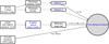 |
Fig. 1 Data flow for fitting time response model parameters. |
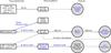 |
Fig. 2 Data flow for determining the HFI beams. |
2. Time response
In Planck’s early data release, a 10-parameter model TF10 describes the time response of the bolometer/electronics system (Planck HFI Core Team 2011a). This section describes an improved model of the time response based on the HFI readout electronics schematics which more accurately reproduces phase shifts in the system close to the Nyquist frequency. The improved model also provides more degrees of freedom for the bolometer’s thermal response in order to describe more accurately the low frequency response of the bolometer.
2.1. Model
The new model is named LFER4 (Low Frequency Excess Response with four time constants) and
consists of an analytic model of the HFI readout electronics (Lamarre et al. 2010) and four thermal time constants and associated
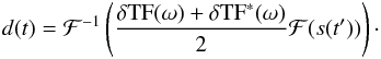
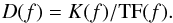
amplitudes for the bolometer:  (1)where TF(ω) represents the full
time response as a function of angular frequency ω. The time response of the
bolometer alone is modelled by
(1)where TF(ω) represents the full
time response as a function of angular frequency ω. The time response of the
bolometer alone is modelled by 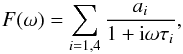 (2)and H′(ω;Sphase,τstray)
is the analytic model of the electronics transfer function (whose detailed equations and
parameters are given in Appendix A) with two
parameters.
(2)and H′(ω;Sphase,τstray)
is the analytic model of the electronics transfer function (whose detailed equations and
parameters are given in Appendix A) with two
parameters.
The overall normalization of the transfer function is forced to be 1.0 at the signal frequency of the dipole, leaving a total of 9 free parameters for each bolometer.
The sum of single-pole low-pass filters represents a lumped-element thermal model with four elements. The thermal model underlying the temporal transfer function is described elsewhere (Spencer et al., in prep.); this work adopts an empirical approach to correcting the data.
The two parameters of H′ mainly affect the high frequency portion of the time response. Sphase represents the phase difference between the bias and the lock-in summation, and is fixed in the model as a readout electronics setting. The second parameter τstray is the time constant of the bolometer resistance and the parasitic capacitance of the wiring and is measured independently during the checkout and performance verification (CPV) phase of the mission prior to the sky survey. All resistance and capacitance values of the readout electronics chain are fixed at values from the circuit diagram.
The in-flight data are used to determine the remaining seven free parameters. Low frequency parameters are constrained by minimizing the difference between the first and second survey maps (Sect. 2.2), while planetary observations are used to constrain those parameters governing the high frequency portion of the time response (Sect. 2.3).
The fastest thermal time constants in the LFER4 model roughly correspond to the time constants measured during pre-launch tests of the bolometers (Holmes et al. 2008; Pajot et al. 2010). The slower time constants contribute lower frequency response at the several percent level. The time constants in the LFER4 model are not exactly identical to those measured on glitches (Planck Collaboration X 2014) due to additional filtering applied by the deglitching. A future publication (Spencer et al., in prep.) will relate the time constants and amplitudes to the thermal properties of the bolometer and module.
2.2. Fitting slow time constants with galaxy residuals
As Planck scans across the Galactic plane, the low frequency time response of HFI spreads Galactic signal away from the plane. Surveys 1 and 2 consist of roughly six months of data each and cover nearly the same sky, scanned at almost opposite angles. The difference between maps made with data from the two individual surveys highlights the effect since the Galactic power is spread in different directions in the two surveys, creating symmetric positive and negative residuals in the difference map. The LFER4 parameters are varied to minimize the difference between these surveys. For most bolometers, the fit is limited to the slowest time constant and its associated amplitude, and in others the fit is extended to the two slowest time constants and associated amplitudes.
Other systematic effects can confuse the measurement of LFER4 parameters by creating a similar positive/negative residual pattern in the survey difference. The philosophy employed here is to minimize the survey residuals fitting only for LFER4 parameters, but to use simulations and data selections to test the dependency of the results with other systematics.
2.2.1. Survey difference method 1
Two techniques are used to perform the fit. The first method is based on map
re-sampling in the time domain, using the pointing to generate synthetic TOI. The
synthetic TOI of each survey is compared with the synthetic TOI of both surveys
combined. Before the production of these synthetic TOI, the maps are smoothed to
30′. Given the fact that
in consecutive surveys the scan direction is nearly opposite, the survey 2 TOI is very
similar to the time-reversal of the survey 1 TOI. This symmetry is assumed to be exact,
ensuring that time reversal is equivalent to taking the complex conjugate in the
frequency domain. Since the sky signal has been convolved by the true transfer function,
TFtrue(ω), and deconvolved by the
estimated – not fully correct – transfer function TF0(ω), the
single survey re-sampled time-stream is
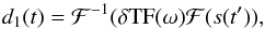
 (3)where ℱ is the Fourier transform operator,
s is the
true sky map observed at time t′, and d1 is the
synthetic TOI. This can be written as,
(3)where ℱ is the Fourier transform operator,
s is the
true sky map observed at time t′, and d1 is the
synthetic TOI. This can be written as,
 (4)having defined δTF(ω) =
TFtrue(ω)/TF0(ω)
as the corrective factor which should be applied to the estimated transfer function. The
synthetic TOI of survey 2, d2, is similarly defined. For the TOI
of both surveys combined, the average of the two maps is used.
(4)having defined δTF(ω) =
TFtrue(ω)/TF0(ω)
as the corrective factor which should be applied to the estimated transfer function. The
synthetic TOI of survey 2, d2, is similarly defined. For the TOI
of both surveys combined, the average of the two maps is used.
Using the time reversal property, the synthetic TOI d(t) of
the full sky map (survey 1 and survey 2 combined) may be written as
 In the Fourier domain, the ratio of the
TOIs is
In the Fourier domain, the ratio of the
TOIs is 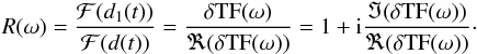 Since the real part of the transfer
function at low frequency is close to 1, the imaginary part of the ratio of the
synthetic beams is equal to the imaginary part of the corrective factor, δTF(ω):
Since the real part of the transfer
function at low frequency is close to 1, the imaginary part of the ratio of the
synthetic beams is equal to the imaginary part of the corrective factor, δTF(ω):
 The LFER4 model of the transfer function is
fitted to this measure of the imaginary part of the correction to infer the parameters
of the true transfer function, in the low frequency regime, typically below a few Hz.
The LFER4 model of the transfer function is
fitted to this measure of the imaginary part of the correction to infer the parameters
of the true transfer function, in the low frequency regime, typically below a few Hz.
2.2.2. Survey difference method 2
The second method looks at one-dimensional slices through the Galactic plane for each survey independently. A sky signal slice is obtained by resampling a sky map for a single survey and a single bolometer. The slices are taken along the scan direction and the sky signal is averaged over 5° in longitude. Only the sky region close to the Galactic plane is considered (10° above and below the Galactic plane and longitudes between −40° and 60°). The slice is convolved with the ratio of the transfer function used to create the map and a new LFER4 transfer function with trial parameter values. New sky survey maps are obtained by re-projecting the slices into pixelized maps. As for the previous method, parameters of the low-frequency part of the LFER4 transfer functions are chosen so that they minimize the residuals in the difference between surveys 1 and 2.
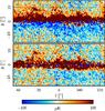 |
Fig. 3 Survey 2 minus Survey 1 residual close to the Galactic centre before (upper) and after (lower) fitting and deconvolving the low frequency part of the time response for bolometer 353-2. Remaining residuals are dominated by gain difference between the surveys due to ADC non-linearity (Planck Collaboration VIII 2014) and artifacts of the different scanning directions (beam asymmetry) and pixel coverage survey to survey. |
In practice, the first method is used for the 100–353 GHz bolometers, and at 545 GHz and 857 GHz the second method is used, being better adapted to the maps having the most structure in the Galactic difference residuals. Figure 3 shows an example of the residual remaining in a HEALPix2 map (Górski et al. 2005) of the survey difference, after fitting the long time response, showing reduced asymmetry in the Galactic plane.
2.2.3. Survey difference systematics
In the survey difference solution for the time response, any systematic effect that creates a residual in the survey difference can be confused with a time response effect, in particular affecting the low frequency time response. This section identifies a number of residual-producing systematics and quantifies the resulting bias in the transfer function. These residual-producing systematics include far sidelobes, zodiacal light, pointing offset uncertainty, gain drifts, main beam asymmetry and polarized sky signal.
Due to the very high signal-to-noise ratio of Galactic signal at sub-millimetre wavelengths, far sidelobe pickup of the Galactic plane is detected in the 545 GHz and 857 GHz channels. A physical optics model of the far sidelobe pickup is used to estimate the signal from the Galactic centre. The optical depth of the zodiacal dust cloud along the line of sight varies as Planck orbits the Sun, leaving a residual in the survey difference (Planck Collaboration XIV 2014). A model of the zodiacal dust emission is subtracted in the reconstruction of the time response. The reconstruction of the time response is then repeated without subtracting the models; these do not significantly affect the result (Fig. 4).
As a probe of the effect of far sidelobes on the time constant determination, the pipeline is run on a survey difference map obtained from the sidelobe model alone for each of the 100, 143, 217, and 353 GHz channels. The method did not find a long time constant, as the sidelobe effect on the survey map is very different from the time constant effect.
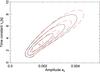 |
Fig. 4 68%, 95%, and 99% likelihood contours for the long time constant τ3 and associated amplitude a3 for a 545 GHz bolometer (545-4) with (black) and without (red) zodiacal emission and far sidelobe removal. The square and cross indicate the maximum likelihood values. |
A systematic offset in the pixel pointing creates a residual in the survey difference. The pointing solution reduces the pointing error to a few arcseconds RMS in both the co-scan and cross-scan direction. With the 6° s-1 scanning speed, this error corresponds to frequencies greater than 1 kHz, far from the range affected by the long time constant.
Gain variability can also bias the estimation; due to non-linearity in the analogue to digital converters (ADC), the HFI responsivity to the sky signal varies at a few tenths of a percent throughout the mission. As a probe of this effect, gain-corrected data for the 100, 143 and 217 GHz bolometers are used to reconstruct the long time response. This has a negligible impact on the fitted parameters. Residual gain errors tend to leave monopolar residuals that are not coupled to the long time constants in the fitting procedure.
Some residual is expected in the survey difference maps because the asymmetric beam scans the sky at different angles in the two surveys. This is especially an issue at 545 GHz where the beam is substantially asymmetric. To quantify the amplitude, simulated survey difference maps are generated using a realistic asymmetric beam model convolved with the Planck Sky Model (Delabrouille et al. 2013); the residuals in the Galactic plane at 545 GHz are dominated by the main beam asymmetry (see Fig. 5).
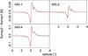 |
Fig. 5 Survey 1 minus survey 2 residual for the 545 GHz bolometers, averaged from Galactic longitude 0 through 20°. The black curves show the Planck data, and red is a simulation. |
Polarization sensitive bolometers (PSBs) show an additional residual in the survey difference maps because of polarized sky signal observed at slightly different crossing angles in the two surveys. For the PSBs, the low frequency time response is therefore determined using different levels of polarization masking. These studies do not suggest the presence of any significant level of bias from polarization, but only higher noise with wider masking. As an additional check on the contribution of residual polarization to the low frequency response, the survey difference of the sum of the two arms of each PSB pair is input to the pipeline. This sum is not sensitive to polarization, and no bias is found in the determination of the time response.
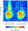 |
Fig. 6 Gridded Jupiter data for bolometer 143-3b before and after fitting for LFER4 parameters. The best fit Gaussian is subtracted from each plot to emphasize residuals. Residuals in the main beam show the deviation from a Gaussian shape, captured in the representations of the scanning beam, as described in Appendices B and C. |
2.3. Fitting fast time constants with planet crossings
Filtering of the TOIs and errors in the deconvolution kernel results in ringing along the scan direction. The planets Mars, Jupiter and Saturn are high signal-to-noise sources that can be used to minimize this smearing by adjusting the parameters of the LFER4 model. See Sect. 3.1 for a description of the planet data.
In solving for the high frequency portion of the time response, the beam profile is forced to be compact. The optical beam is modelled as a spline function on a two-dimensional grid (see Appendix C for details) and the LFER4 parameters are fit by forcing conditions on the resulting beam shape (Fig. 6).
The planet data are first deconvolved with a time response model derived from pre-launch data, to recover an initial estimate of the beam profile. Jupiter is used for the 100, 143 and 217 GHz channels, while Saturn is used for higher frequencies (see Sect. 3.4 for a discussion of the non-linearity of Jupiter at higher frequencies).
Rather than deconvolve the planet data, the model parameters are determined in the forward sense. Since the beam is decomposed into B-spline functions, this basis is convolved with the temporal transfer function to retrieve the coefficients for each basis function using the planet data. These coefficients are applied to the original deconvolved B-spline functions to recover an estimate of the optical beam. The convolution is made in the Fourier domain by re-sampling the B-spline function onto a timeline with a sample separation corresponding to 4.̋5. The typical knot separation length of the basis function is between 1′ and 2′.
In the Fourier domain, the convolution of the temporal transfer function with the planet
signal is 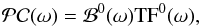 (5)where ℬ0(ω) is the
Fourier transform of the slice through the peak planet signal in the scan direction
b0(t), which is
obtained by de-convolving planet data using a fiducial estimate, TF0(ω) of the
transfer function. The slice b0(t) is then
symmetrized about the origin (defined by the location of the maximum of the
B-spline
representation)to obtain bsym(t), and its
Fourier transform ℬsym(ω). This operation aims to recover
a beam that, by construction, is symmetric, within the limits allowed by the model of the
temporal transfer function,
(5)where ℬ0(ω) is the
Fourier transform of the slice through the peak planet signal in the scan direction
b0(t), which is
obtained by de-convolving planet data using a fiducial estimate, TF0(ω) of the
transfer function. The slice b0(t) is then
symmetrized about the origin (defined by the location of the maximum of the
B-spline
representation)to obtain bsym(t), and its
Fourier transform ℬsym(ω). This operation aims to recover
a beam that, by construction, is symmetric, within the limits allowed by the model of the
temporal transfer function, 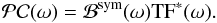 (6)Here ℬsym(ω) is
entirely defined by
(6)Here ℬsym(ω) is
entirely defined by  and TF0(ω) and the new estimate of the time
response TF∗(ω) is derived from Eq. (6). This function is parameterized in terms of
the three shortest time constants (τ1, τ2,
τ3) and their associated amplitudes
(a1,a2,a3).
and TF0(ω) and the new estimate of the time
response TF∗(ω) is derived from Eq. (6). This function is parameterized in terms of
the three shortest time constants (τ1, τ2,
τ3) and their associated amplitudes
(a1,a2,a3).
2.4. Stationarity of the time response
The time response of each HFI detector/readout channel is a function of the cryogenic temperature of the bolometers and the ambient-temperature components of the readout electronics. Both cryogenic and ambient temperatures change throughout the mission as the Galactic particle flux and the Planck spacecraft solar distance are modulated. The seasonal consistency of the scanning beam sets an upper limit on changes in the time response through the mission, shown below in Sect. 5.2.1.
2.5. Deconvolution of the data
The time response transfer function is deconvolved from the data and not included as part of the scanning beam, because the low frequency response of the bolometer would give an extended scanning beam, stretching many degrees from the main lobe along the scan direction.
Since the time response amplitude decreases as a function of frequency, the deconvolution operation increases the noise at high frequency to an unacceptably high fraction of the RMS. During the deconvolution stage of the TOI processing, a phaseless low-pass filter is applied in order to suppress the high frequency noise and keep pixel aliasing at a manageable level.
In the early data release, a finite impulse response low-pass filter was used for this
purpose (Planck HFI Core Team 2011b). In the 2013
cosmology data release, the low-pass filter is further tuned for the 100, 143, 217 and 353
GHz channels to reduce filter ripple produced by the lowpass filters used in the
early-release data. The filter is now implemented in the Fourier domain, with a kernel
consisting of the product of a Gaussian and a squared cosine,  (7)where
 (8)and
 (9)Here fmax =
fc +
k(fsamp/2 −
fc) and fsamp is the
sampling frequency of the data. The parameters of the filter are the same for all
bolometers in the bands 100–353 GHz: fGauss = 65 Hz; fc = 80 Hz; and
k = 0.9. To
first order, this filter widens the scanning beam along the scan in an equivalent way to
convolving the optical beam with a Gaussian with full-width at half-maximum (FWHM) of
2.́07. The filter introduces some rippling along the scan direction at the −40 dB level at 217 and 353 GHz, where the
beams allow harmonic signal content close to the filter edge. The rippling is captured by
the B-spline
beam representation (see Fig. 11).
(9)Here fmax =
fc +
k(fsamp/2 −
fc) and fsamp is the
sampling frequency of the data. The parameters of the filter are the same for all
bolometers in the bands 100–353 GHz: fGauss = 65 Hz; fc = 80 Hz; and
k = 0.9. To
first order, this filter widens the scanning beam along the scan in an equivalent way to
convolving the optical beam with a Gaussian with full-width at half-maximum (FWHM) of
2.́07. The filter introduces some rippling along the scan direction at the −40 dB level at 217 and 353 GHz, where the
beams allow harmonic signal content close to the filter edge. The rippling is captured by
the B-spline
beam representation (see Fig. 11).
The 3-point finite impulse response filter is still used for the 545 and 857 GHz channels3. This extends the scanning beams along the scan direction more than the Gaussian-cosine Fourier filter (the 545/857 GHz filter time scale corresponds to 3.́0 on the sky), but has the advantage of reducing rippling and signal aliased from above the Nyquist frequency.
The deconvolution kernel multiplied by the data in the Fourier domain is the product of
the lowpass filter with the inverse of the bolometer/electronics time response,
 (10)Figure 7
shows a comparison of the deconvolution functions resulting from the LFER4 model and from
the TF10 model used in the ERCSC data. The differences between the two models appear
mainly in the phase at high frequency, mostly above the signal frequency corresponding to
the beam size. Although the phase of LFER4 is a more accurate description of the system,
in practice replacing LFER4 with TF10 had little effect on the data, because of the
lowpass filter applied at the time of deconvolution and the empirical determination of an
overall sample offset in the pointing reconstruction.
(10)Figure 7
shows a comparison of the deconvolution functions resulting from the LFER4 model and from
the TF10 model used in the ERCSC data. The differences between the two models appear
mainly in the phase at high frequency, mostly above the signal frequency corresponding to
the beam size. Although the phase of LFER4 is a more accurate description of the system,
in practice replacing LFER4 with TF10 had little effect on the data, because of the
lowpass filter applied at the time of deconvolution and the empirical determination of an
overall sample offset in the pointing reconstruction.
In the HFI data processing (Planck Collaboration VI 2014), data chunks of length 219(≈5 × 10⁵) samples are Fourier transformed at a time, overlapping by half with the subsequent chunk to avoid edge effects.
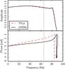 |
Fig. 7 Phase and amplitude as a function of signal frequency of the deconvolution function of bolometer 217-1. The solid black curve is the LFER4 model, while the dashed red curve shows the TF10 model used in the earlier Planck papers. The vertical dotted line marks the signal frequency corresponding to the half power point of the average effective beam. |
3. Scanning beams
The filtering of the TOI and the accuracy of the deconvolution kernel affect the angular response of the HFI detectors. An accurate estimate of the scanning beam, resulting from the filtering of the physical (optical) beam by these time domain convolutions, is required to relate the angular power spectra of the maps to that of the underlying sky. As described in Planck HFI Core Team (2011a) and Planck HFI Core Team (2011b), the HFI scanning beam profiles are measured using the planetary observations. HFI uses two flat sky representations of the two-dimensional scanning beams, one using Gauss-Hermite polynomials, and another using B-spline functions.
Three selections of planetary data are used to derive estimates of different aspects of the beam:
-
1.
the first two observing seasons of Mars (main beam, andwindow functions);
-
2.
all available seasons of Mars [3], Jupiter [5] and Saturn [4] (near sidelobe); and
-
3.
all five Jupiter observations (residual time response).
The effective beam window functions used in the CMB analysis are ultimately derived from the first of these. In each case, the statistical properties of the beam representations and the choice of planetary data are studied using ensembles of simulated planet observations (Sect. 5).
While the signal-to-noise ratio of the Jupiter and Saturn data is significantly greater than the Mars data, at this stage of the analysis a reconstruction bias results in the main beams recovered from simulated Jupiter and Saturn observations that is not present in the simulations of Mars. Additionally, the non-linear response of some HFI detectors to the Jupiter signal (Planck HFI Core Team 2011a) makes the normalization of the planet peak response uncertain at the few percent level (see Sect. 3.4). Therefore the main beam model is established using Mars data, while observations of Jupiter and Saturn are used only to estimate the near sidelobes and residuals in the deconvolution of the transfer function.
The B-spline representation of the joint Mars observations is used as input for the calculation of the effective beam and the effective beam window function. Simulations have shown the B-spline representation to better capture the features outside of the main lobe, due to the necessarily finite order of the Gauss-Hermite decomposition. However, the Gauss-Hermite model is used for other systematics checks, including the consistency of the planets and observing seasons.
Because the Jupiter and Saturn data allow measurement of the beam response below −45 dB from the peak, there is no need to rely on a model of the telescope to determine the main beam or near sidelobe structure.
3.1. Planetary data handling
The JPL Horizons package4 (Giorgini et al. 1996) is programmed with Planck’s orbit to calculate the positions of the planets. Table 1 shows the dates when the planets were within 2° of the centre of the focal plane. By the end of HFI operations Mars was observed three times, Saturn four times, and Jupiter five.
The planets Jupiter, Saturn and Mars are among the brightest compact objects seen by Planck HFI; the signal amplitude affects the data handling in a number of ways. Moving solar system objects are flagged and removed from the TOI in the standard processing pipeline. Specialized processing for the planet data is required, with two major differences from the nominal processing (see Planck Collaboration VI 2014 for details).
Observation seasons of the planets observed by Planck: date range and position in Galactic coordinates.
While the pickup from the 4He-JT cooler is removed from the data as usual, pointing periods containing very bright sources such as the planets cannot be used to reliably estimate the line amplitude. Instead, during the planet observations, these are extrapolated from neighbouring pointing periods.
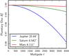 |
Fig. 8 Window functions of the planetary discs of Jupiter, Saturn, and Mars, equivalent to the bias in the inferred effective beam window function if the beam is reconstructed from observations of one of these planets alone. The labels show the corresponding angular radius of each disc. |
To better detect glitches near the extremely bright planet crossings, an estimate of the planet signal is subtracted from the data prior to glitch detection. Glitch template subtraction is performed on the signal-subtracted timeline in the same way as during nominal observations.
In order to remove the (quasi-stationary) astrophysical background from the planetary data, a bilinear interpolation of the frequency averaged map is subtracted. The full mission map is used for the five-season Jupiter data, while the nominal survey sky maps are used in the processing of the other planetary data.
The planets are oblate spheroids, and appear as ellipses slightly extended along the direction of the ecliptic. The Planck planet range and Planck sub-latitude calculated by JPL Horizons are used in combination with the polar and equatorial radii of the planets reported by Horizons to compute the angular size and ellipticity of each planet. During HFI observations, the mean angular radii of Jupiter, Saturn and Mars are 20.̋44, 8.̋542, and 4.̋111, respectively. The ratio of the equatorial to polar radii are 1.069, 1.109 and 1.006, respectively.
The finite planetary disc size increases the apparent size of the scanning beam and
biases the inferred effective beam window function. The filtering in multipole space of a
circular disc of angular radius R can be written as Bdisc(ℓ) =
2J1(ℓR)
/(ℓR), where J1(x) is the Bessel
function of order 1. Figure 8 shows the
 for the three planetary discs. In
practice, the effects of the disc size are mitigated by merging observations from the
three brightest planets. The effects of the large Jupiter disc size are greatest where the
spatial gradient of the beam is greatest, between the –3 to −10 dB contours of the beam. By excluding
the Jupiter observations above −
10 dB, the disc size smearing is reduced, and setting a −20 dB threshold results in a bias in the
window function below 10-3 at all multipoles.
for the three planetary discs. In
practice, the effects of the disc size are mitigated by merging observations from the
three brightest planets. The effects of the large Jupiter disc size are greatest where the
spatial gradient of the beam is greatest, between the –3 to −10 dB contours of the beam. By excluding
the Jupiter observations above −
10 dB, the disc size smearing is reduced, and setting a −20 dB threshold results in a bias in the
window function below 10-3 at all multipoles.
Planck observes Saturn at a range of ring inclination angles: 6.̊03, 2.̊45, 12.̊6 and 9.̊4 for seasons 1, 2, 3 and 4, respectively. While emission from the solid angle of the ring increases the effective planetary disc area, the brightness temperature of the ring tends to be much less than the planetary disc temperature for the Planck bands. For example Weiland et al. (2011) fit a single 90 GHz ring brightness temperature 14% that of the Saturn disc. In our beam reconstruction the average of the first three Planck observations of Saturn is used, and even in the extreme limit where the ring brightness temperature is the same and only Saturn data are used, the multipole space correction is 2 × 10⁻³ at ℓ = 3000; this correction is ignored.
The elliptical shape of the planetary disc gives a further bias in the inferred window function, depending on whether the long axis of the beam is aligned with or perpendicular to the long axis of the planet. In this case the planetary disc is approximated as an elliptical Gaussian with σ = 0.5R. The worst case is a 10-3 effect in the case of 100 GHz beams measured on Jupiter at ℓ = 3000 (where the 100 GHz window function is vanishingly small). At 143 and 217 GHz, the 10-3 level is reached only at ℓ = 4000. The effect is negligible in the range of Planck’s sensitivity. With Saturn and Mars, the ellipticity effects are <10-4 and <10-6, respectively, at all multipoles; the ellipticity of the planetary discs has a negligible effect on the estimate of the scanning beam.
3.2. Main beam model
Two representations are used to describe the (two dimensional) main beam; a Gauss-Hermite basis (described in Appendix B following Huffenberger et al. 2010 and Planck HFI Core Team 2011a) and a B-spline basis (Appendix C).
The Gauss-Hermite (GH) and B-spline bases have very different characteristics. The GH representation uses a relatively small number of parameters and, in practice, amounts to a perturbative expansion about a Gaussian shape. The B-spline is quite general, using many more degrees of freedom to fit the data on a defined grid, with the spline controlling the behaviour in between. The bias and correlation structure of the noise of these two representations are characterized using Monte Carlo simulations of the planetary data which include all the details of the beam-processing pipeline used on the data (these simulations are described more completely in Sect. 5). In each case, the parameters of the representation are derived directly from the time-ordered data, without recourse to a pixelized map.
Figure 9 shows the B-spline scanning beams for the entire HFI focal plane, as reconstructed from the Jupiter and Saturn data. Figure 10 shows the radially binned, frequency averaged beam profile for the HFI channels, comparing the B-spline representation of the Mars data (solid black lines) with the combined Mars, Jupiter and Saturn data (filled and open points, and the blue dashed line). The B-spline maps are apodized with a Gaussian at a radius beyond the signal-to-noise floor of the Mars data: 13.́4, 13.́0, 11.́4, 12.́9, 17.́8, 17.́8 on average at 100, 143, 217, 353, 545,and 857 GHz respectively.
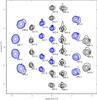 |
Fig. 9 B-spline scanning beams reconstructed from Mars, Saturn, and Jupiter seasons 1, 2 and 3 data for near sidelobe studies. The beams are plotted in logarithmic contours of − 3, − 10, − 20 and − 30 dB from the peak. PSB pairs are indicated with the a bolometer in black and the b bolometer in blue. |
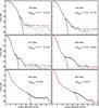 |
Fig. 10 Azimuthally- and band-averaged main beam profiles (black solid curve) derived from the B-spline representation of the first and second Mars observations compared to that derived from a combination of Mars, Jupiter and Saturn observations (filled and open markers represent positive and negative data respectively). The red dashed line is defined as the joint envelope of the main beam and near sidelobe dataset, the integral of which represents the maximal solid angle that is compatible with these data. A nominal near lobe model, provided as a reasonable extrapolation of the data below the noise floor, is shown as the blue dashed line. The fractional increase in solid angle, relative to the Mars-alone derived beam profile, is displayed in each panel. The black dotted line shows the GRASP physical optics model averaged over a subset of detectors that have been simulated (100–353 GHz). The data show a clear excess in power over the model at 143, 217 and 353 GHz that is consistent with a spectrum of surface errors on scales between 2 and 12 cm, with an RMS of order 10 μm. Table 2 contains an estimate of the fraction of the solid angle in the near sidelobes that is not captured in the B-spline representation. For clarity, the figure extends only to 45′. In all cases the solid angle is derived from the profile extending out to 5°. Due to the high signal-to-noise of the Jupiter data (− 40 to − 55 dB, depending on the frequency), and the rapidly falling response of the beam, the solid angle estimates are insensitive to the limit of integration. |
The azimuthally averaged beam window function,  , from each of these models is compared to
the known input beam model. At 100, 143 and 217 GHz the two methods perform comparably,
with the B-spline having slightly smaller bias and variance; at
the higher frequencies the B-spline performs demonstrably better, especially at
545 and 857 GHz, as expected due to the highly non-Gaussian shape of these multi-mode
detectors.
, from each of these models is compared to
the known input beam model. At 100, 143 and 217 GHz the two methods perform comparably,
with the B-spline having slightly smaller bias and variance; at
the higher frequencies the B-spline performs demonstrably better, especially at
545 and 857 GHz, as expected due to the highly non-Gaussian shape of these multi-mode
detectors.
3.3. Near sidelobes
While the HFI beams are Gaussian at the −25 dB level, non-trivial structure in the beam is captured in the data at lower power. There are two distinct components to the near lobe response: a discrete pattern of secondary lobes evident at frequencies of 217 GHz and above; and a diffuse shoulder consistent with phase errors in the aperture plane.
The Planck reflectors suffer from print-through of the honeycomb
structure that supports the carbon-fiber face sheets. The size of the deformation has been
measured during thermal testing to be less than 20 μm (Tauber et al.
2010). While small in amplitude, the strict periodicity of this pattern results
in a correspondingly periodic structure in the near lobes, seen clearly in Fig. 12, which is slightly larger than predicted based on the
pre-launch measurements. A simple grating equation describes the angular positions of the
resulting contributions to the near sidelobes, 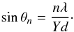 (11)where θn is the angular
position of the order n lobe from the central beam peak, λ is the wavelength of the
radiation, d
is the grating periodicity and Y is a factor that describes the position of each
reflector along the optical path, with Y = 1.00 for the primary reflector and
Y = 1.80
for the secondary reflector. Three possible periodicities (19.6 mm, 30 mm, 52 mm) in the
honeycomb array dominate the Planck dimpling pattern for the 857 GHz
detectors, though only those for the 52 mm periodicity can be seen for the 545 GHz and 353
GHz detectors. For the highest frequency detectors, only the weaker lobes due to the 19.6
mm and 30 mm periodicities are seen outside the 40′ main beam model, but they contribute at
most (0.050 ± 0.008)% to the
integrated beam solid angle. A forthcoming publication (Oxborrow et al., in prep.) will
present an in-depth study of the mirror surface.
(11)where θn is the angular
position of the order n lobe from the central beam peak, λ is the wavelength of the
radiation, d
is the grating periodicity and Y is a factor that describes the position of each
reflector along the optical path, with Y = 1.00 for the primary reflector and
Y = 1.80
for the secondary reflector. Three possible periodicities (19.6 mm, 30 mm, 52 mm) in the
honeycomb array dominate the Planck dimpling pattern for the 857 GHz
detectors, though only those for the 52 mm periodicity can be seen for the 545 GHz and 353
GHz detectors. For the highest frequency detectors, only the weaker lobes due to the 19.6
mm and 30 mm periodicities are seen outside the 40′ main beam model, but they contribute at
most (0.050 ± 0.008)% to the
integrated beam solid angle. A forthcoming publication (Oxborrow et al., in prep.) will
present an in-depth study of the mirror surface.
The second component is a beam shoulder becoming significant near the −30 dB contour, and extending to 2–4 FWHM from the beam centre. This shoulder is consistent with scattering from random surface errors on the primary and secondary reflectors, and is reasonably well-described by a spectrum of surface errors with correlation lengths ranging from 2 to 12 cm, with an RMS of order 10 μm (Ruze 1966). The contribution of each of these components is included in the radially binned profiles shown in Fig. 10.
While the B-spline parameterization captures both the main beam and near sidelobe structure, the extended features must be separately included in the Gauss-Hermite beam representation. Figure 11 shows contour plots of a B-spline beam using Mars, Jupiter and Saturn data at each frequency.
The B-spline representation of the scanning beam used to compute the window function includes only that portion of the near sidelobe structure that falls within the signal-to-noise of the Mars data; the Jupiter and Saturn data provide an estimate of the beam solid angle that is neglected in the scanning beam product. The near sidelobe solid angle, and the resulting window function error, are sensitive to the details of the analysis, including the sky subtraction, offset removal and masking of in-scan ringing at the part-per-million level. Although a comprehensive study of these effects in the Jupiter and Saturn data are underway, a conservative, and model independent upper limit is obtained by taking the envelope of the noise floor to define the maximum solid angle allowed by the data (the red dashed line in Fig. 10). A reasonable estimate of the true solid angle in the near lobes can be obtained by extrapolating the data below the noise floor (the blue dashed line in Fig. 10). By either measure, the grating lobes and diffuse shoulder account for a small fraction of the total beam solid angle; for the 100, 143 and 217 GHz channels this contribution represents less than 0.15% of the total solid angle (see Table 2). The amplitude of the impact on the window function is estimated by comparing the Legendre transform of the maximal envelope of the Jupiter and Saturn data with that of the nominal Mars derived scanning beam. The result is shown as the family of green curves in Fig. 19. Because the Monte Carlo ensembles that are used to derive the error envelope neglect this near sidelobe structure in the beam that is input to the simulations, the window function error amplitudes have been scaled to accomodate the upper limit defined by the noise floor of the Jupiter and Saturn data.
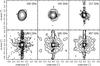 |
Fig. 11 One scanning beam at each HFI frequency (100-3b, 143-6, 217-1, 353-7, 545-1, and 857-3). Contours are in dB from the peak in steps of −5 dB. The lowest contours are set at −30 dB, −35 dB, −40 dB, −45 dB, −45 dB, −45 dB at 100 GHz, 143 GHz, 217 GHz, 353 GHz, 545 GHz, and 857 GHz, respectively. |
Scanning beam solid angle (ΩSB) error budget, showing the bias and fractional error due to the residual time response (ΔΩτ), near sidelobes (ΔΩNSL) and solid angle colour correction (ΔΩCC).
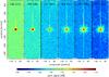 |
Fig. 12 Gridded data from all five seasons of Jupiter. The colour scale shows the absolute value of the peak signal. |
3.4. Residual time response
The Planck spacecraft spin rate is constant to 0.1%, making the time response of the electronics and the bolometer degenerate with the angular response of the optical system.
The B-spline beam model extends ±20′ from the centre of the beam. An error in the time response on fast timescales will thus be exactly compensated by the scanning beam. However, errors in the time response beyond the limit of the scanning beam reconstruction will not be accounted for, and will bias the recovered beam window function.
To look for residual long tails due to incomplete deconvolution of the time response, all five seasons of Jupiter observations are binned into a 2D grid of 2′ pixel size extending 6° from the planet (Fig. 12). These are background-subtracted using the Planck maps and stacked by fitting a Gaussian to estimate the peak amplitude and centroid of each observation. The data are binned as a function of pointing relative to the planet centre.
While a static non-linearity correction is included in the TOI processing, partial ADC saturation and dynamical non-linearity bias the normalization of these tails by underestimating the Jupiter peak signal. An estimate of the non-linear correction is derived by fitting a gridded map of all three Mars observations to a map of all five Jupiter observations for each detector. A signal reduction at the peak of Jupiter is ruled out at the 1% level at 100 and 143 GHz, but detected at higher frequencies. Relative to Mars, the peak Jupiter signal is reduced by non-linearity on average by 3 ± 3%, 12 ± 3%, 12 ± 4% and 65 ± 20% at 217, 353, 545 and 857 GHz, respectively. The tail normalizations are scaled by these factors.
An example of the residual tail is shown in Fig. 13. As well as a tail following the planet due to imperfect deconvolution of the time response, there is also a tail preceding the planet crossing; this is due to the lowpass filter applied in the Fourier domain. The residual beam tails have amplitudes typically at the level of 10-4 of the peak but extend several degrees from the centre of the beam. The response beyond 6° on the sky is consistent with noise for all detectors.
The signal to noise of the tail measurement greater than 6° from Jupiter sets a model-independent limit on the knowledge of the time response at signal frequencies from 0.016 Hz to 0.1 Hz at <10-4.
These stacked Jupiter data are integrated to determine the expected bias in total beam solid angle from this remaining uncorrected time response (see Table 2). The mean integral values are typically a few times 10-4 of the main beam solid angle, an order of magnitude lower than the error in the beam solid angle due to noise and other systematics.
The residual scanning beam tails can also bias the effective beam window function. The
spherical harmonic transform of the residual that is not included in the model for the
main scanning beam is computed,  , where
 is the multipole space representation of
the main scanning beam model and
is the multipole space representation of
the main scanning beam model and  is the multipole space representation of
the long tail model. In all cases, the m = 0 (symmetric) mode of the ratio of
is the multipole space representation of
the long tail model. In all cases, the m = 0 (symmetric) mode of the ratio of
 to dominates higher order modes by at least a
factor of 1000, meaning that the coupling to the scan strategy is negligible and the bias
in the effective beam window function can be approximated by
to dominates higher order modes by at least a
factor of 1000, meaning that the coupling to the scan strategy is negligible and the bias
in the effective beam window function can be approximated by
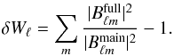 (12)The main effect on the effective beam window
function is that at low ℓ, the bias δWℓ
approaches a value of twice the fractional contribution to the total solid angle. When the
window function is normalized to unity at the dipole frequency, the effect is a roughly
constant bias in the window function at a level of a few × 10-4 for ℓ > 100. The contribution
of the residual tail to the window function is neglected in the error budget.
(12)The main effect on the effective beam window
function is that at low ℓ, the bias δWℓ
approaches a value of twice the fractional contribution to the total solid angle. When the
window function is normalized to unity at the dipole frequency, the effect is a roughly
constant bias in the window function at a level of a few × 10-4 for ℓ > 100. The contribution
of the residual tail to the window function is neglected in the error budget.
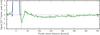 |
Fig. 13 A slice through stacked Jupiter data for bolometer 143-6, illustrating residual long time response after deconvolution. The vertical dotted line shows the extent of the scanning beam map (plotted in blue). |
3.5. Far sidelobes
The far sidelobes (FSL) are defined as the response of the instrument at angles more than 5° from the main beam centroid. Tauber et al. (2010) describes the pre-launch measurements and predictions of the far sidelobe response using physical optics models. Figure 14 compares the measured beam profile of detector 353-1 with the FSL physical optics model. The way the FSL are treated in the dipole calibration and in the scanning beam model affects the effective beam window function, and care is needed to check whether the off-axis response could bias the window function at ℓ > 40 (angular scales 5°) relative to ℓ< 40. To the extent that the physical optics simulations correctly predict the far sidelobe response (which is shown to be roughly the case in the survey difference maps), they produce effects negligible in the effective beam window function of HFI. Appendix D presents the details of this calculation.
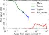 |
Fig. 14 Azimuthally averaged profiles of measured beams of channel 353-1 compared to the azimuthal average of the far sidelobe physical optics model. |
As a check of the quality of the physical optics model of the far sidelobes, Planck Collaboration XIV (2014) attempt a template fit of the physical optics model to the survey difference maps in combination with a zodiacal light model. The template fits are presented in Table 4 of Planck Collaboration XIV (2014). The FSL signature is clearly detected at 857 GHz at a level much higher than predicted. As these channels are multi-moded (Maffei et al. 2010), the differences are not that surprising; it is very difficult to perform the calculations necessary for the prediction. In addition, the specifications for the horn fabrication were quite demanding, and small variations, though still within the mechanical tolerances, could give large variations in the amount of spillover.
For the lower frequency, single-moded channels, there is no clear detection of primary (PR) spillover (i.e., pickup from close to the spacecraft spin axis; see Appendix D). While the significant negative values of the best fit template amplitude may indicate some low-level, large-scale systematic, there seems to be nothing with the distinctive signature of PR spillover at frequencies between 100 and 353 GHz. These values indicate that the PR spillover values in Table 2 of Tauber et al. (2010) may be overestimated.
For the direct contribution of the secondary (SR) spillover, the situation is similar at 353 GHz, but at 217 and 143 GHz there is a 3σ detection at about the level expected, while at 100 GHz the value is about 2.5 times higher than expected, though the signal-to-noise level of the detection is less than 2σ. The baffle contribution to the SR spillover appears higher than predicted, though Planck Collaboration XIV (2014) note that the baffle spillover is difficult to model and the diffuse signal is easily contaminated by other residuals in the survey difference.
Mean values of effective beam parameters for each HFI frequency.
4. Effective beams
Unlike WMAP (Jarosik et al. 2011), for large portions of the sky the scan strategy of Planck does not azimuthally symmetrize the effect of the beams on the CMB map. Treating the beams as azimuthally symmetric leads to a flawed power spectrum reconstruction. To remedy this, the effective beam takes the coupling between the azimuthal asymmetry of the beam and the uneven distribution of scanning angles across the sky into account.
The effective beam is computed for each HFI frequency scanning beam and scan history in real space using the FEBeCoP (Mitra et al. 2011) method, as in Planck’s early release (Planck HFI Core Team 2011b). A companion paper describes the details of the application of FEBeCoP to Planck data (Rocha et al., in prep.).
FEBeCoP calculates the effective beam at a position in the sky by
computing the real space average of the scanning beam over all crossings angles of that sky
position. The observed temperature sky  is a convolution of the true sky
T and the
effective beam ℬ,
is a convolution of the true sky
T and the
effective beam ℬ,
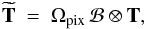 (13)where Ωpix is the solid angle of a pixel,
and the effective beam can be written in terms of the pointing matrix Ati and the scanning beam
(13)where Ωpix is the solid angle of a pixel,
and the effective beam can be written in terms of the pointing matrix Ati and the scanning beam
 as
as 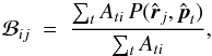 (14)where t is the time-ordered data
sample index and i is the pixel index. Ati is 1 if the pointing direction falls in pixel
number i, else
it is 0, pt represents
the pointing direction of the time-ordered data sample, and
(14)where t is the time-ordered data
sample index and i is the pixel index. Ati is 1 if the pointing direction falls in pixel
number i, else
it is 0, pt represents
the pointing direction of the time-ordered data sample, and
 is the centre of pixel number
j, where the
scanning beam
is the centre of pixel number
j, where the
scanning beam  is being evaluated (if the pointing
direction falls within the cut-off radius).
is being evaluated (if the pointing
direction falls within the cut-off radius).
The sky variation of the effective beam solid angle and the ellipticity of the best-fit Gaussian to the effective beam at HEALPix Nside = 16 pixel centres are shown for 100 GHz in Fig. 15. The effective beam is less elliptical near the ecliptic poles, where more scanning angles symmetrize the beam.
The mean and RMS variation of the effective beam solid angle across the sky for each HFI map are presented in Table 3.
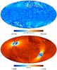 |
Fig. 15 Effective beam solid angle (upper panel) and the best-fit Gaussian ellipticity (lower panel) of the 100 GHz effective beam across the sky in Galactic coordinates. |
4.1. Effective beam window functions
The multipole space window function of one (or two) observed map(s) is defined, in the
absence of instrumental noise and other systematics, as the ratio of the ensemble averaged
auto- or cross-power spectrum of the map(s) to the true theoretical sky power spectrum
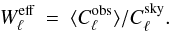 (15)It must account for the azimuthal asymmetry
of the scan history and the beam profile. This is done in the HFI data processing pipeline
using the harmonic space method Quickbeam (described in Appendix
E.2), which allows a quick determination of the
nominal effective beam window functions and of their Monte Carlo based
error eigenmodes (Sect. 6) for all auto- and cross-spectra pairs of HFI detectors, the
error determination being computationally intractable with FEBeCop.
(15)It must account for the azimuthal asymmetry
of the scan history and the beam profile. This is done in the HFI data processing pipeline
using the harmonic space method Quickbeam (described in Appendix
E.2), which allows a quick determination of the
nominal effective beam window functions and of their Monte Carlo based
error eigenmodes (Sect. 6) for all auto- and cross-spectra pairs of HFI detectors, the
error determination being computationally intractable with FEBeCop.
In the FEBeCoP approach, many (approximately 1000) random
realizations of the CMB sky are generated starting from a given fiducial power spectrum
 . For each beam model, the maps are
convolved with the pre-computed effective beams, and the pseudo-power spectra
. For each beam model, the maps are
convolved with the pre-computed effective beams, and the pseudo-power spectra
 of the resulting maps are computed and
corrected by the mode coupling kernel matrix M (Hivon et al.
2002) for a given sky mask:
of the resulting maps are computed and
corrected by the mode coupling kernel matrix M (Hivon et al.
2002) for a given sky mask:  The Monte Carlo average of
kernel-corrected power spectra compared to the input power spectrum then gives the
effective beam window function (Eq. (15),
with replacing
The Monte Carlo average of
kernel-corrected power spectra compared to the input power spectrum then gives the
effective beam window function (Eq. (15),
with replacing
 ).
).
In addition, another harmonic space method (FICSBell; Appendix E.1) was also tested and all three methods give consistent results for the nominal window functions at 100–353 GHz (see Fig. E.1).
For two different maps obtained with different detectors or combination of detectors
X and
Y, because
of the optical beam non-circularity and Planck’s scanning strategy, the
cross-beam window function is not the geometrical mean of the respective auto-beam window
functions, i.e., ![Mathematical equation: \begin{equation} W^{XY}(\ell) \ne \left[W^{XX}(\ell) W^{YY}(\ell)\right]^{1/2} \quad\text{if}\ X \ne Y, \label{eq:crossbeam} \end{equation}](/articles/aa/full_html/2014/11/aa21535-13/aa21535-13-eq164.png) (16)as illustrated in Fig. 16, while of course WXY =
WYX for any
X and
Y.
(16)as illustrated in Fig. 16, while of course WXY =
WYX for any
X and
Y.
The effective beam window functions for the 2013 maps are shown in Fig. 17. Variations in the effective beam window function from place to place on the sky are significant; the published window functions have been appropriately weighted for the analysis of the nominal mission on the full sky. Analyses requiring effective beam data for more restricted data ranges or for particular regions of the sky should refer to the specialized tools provided in Planck Collaboration (2013).
5. Uncertainties and robustness
Ensembles of simulated planetary observations are used to propagate noise and other systematic effects in the time-ordered data into errors in the beam reconstruction. These simulations are also used to estimate bias in the reconstruction of the beam by comparing the ensemble average beam with the input beam.
To assess the completeness of the statistical and systematic noise model, the consistency of the beam reconstruction derived from different planetary observations is measured against corresponding Monte Carlo ensembles. The MC-derived beam statistics, including both the bias and the correlation structure of the errors, have been found to be somewhat sensitive to the near lobe structure that is included in the beam used as an input to the simulations. An investigation of this effect is ongoing.
In addition, several sources of systematic error that can potentially impact the beam determination, but are not included in the current simulation pipeline, have been investigated. The most significant of these are the beam colour correction and distortion due to ADC non-linearity. These errors are estimated separately and found to be small in comparison to the error bars estimated in the eigenmode analysis described in Sect. 6.
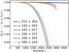 |
Fig. 16 Ratios of the cross-beam window functions |

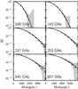 |
Fig. 17 Effective beam window functions (solid lines) for each HFI frequency. The shaded region shows the ± 1σ error envelope. Dashed lines show the effective beam window function for Gaussian beams with FWHM 9.́65, 7.́25, 4.́99, 4.́82, 4.́68, and 4.́33 for 100, 143, 217, 353, 545 and 857 GHz, respectively. |
5.1. Simulation of planet observations
The bias and uncertainty in the scanning beams are determined using ensembles of simulated planet observations. The simulation pipeline uses the LevelS Planck simulation code (Reinecke et al. 2006) to generate simulations of the first two observations of Mars and the first three observations of Jupiter and Saturn for each bolometer. This pipeline is used to generate 100 simulations for each bolometer at 353 GHz, 545 GHz and 857 GHz, 200 at 143 GHz and 217 GHz, and 400 at 100 GHz. Each simulation is reconstructed into a beam model using the identical procedure and software as for the real data.
The components of the simulations are as follows.
-
1.
The scanning beams used as input to the simulations are thesame Mars beams used to calculate the effective beam windowfunction. As shown in Appendix B, thereconstruction bias depends more on the beam representationthan the exact input beam used in a simulation.
-
2.
The Planck spacecraft pointing and the Horizons ephemerides are used to calculate the pointing relative to the planets for the simulation. An additional random 2.̋5 RMS per sample pointing error is added in both the in-scan and cross-scan directions with a power spectral density given by the pointing error estimate, consistent with the estimated error in the spacecraft pointing (see Sect. 4, and Fig. 7 of Planck Collaboration VI 2014). Error in the beam centroid determination is not simulated.
-
3.
Detector noise is generated in the timeline by a random realization of Gaussian noise with a power spectral density as reported in Planck Collaboration VI (2014).
For a small number of the simulations, cosmic ray glitches are added to the simulation with the energy spectrum and rate measured in the data (Planck Collaboration X 2014), and the deglitching procedure from the standard pipeline is applied to detect samples contaminated by glitch transients and to subtract the long tails (Planck Collaboration VI 2014).
Each simulation in the ensemble provides an estimate of the scanning beam, which is then used as input to Quickbeam (Appendix E.2) to estimate an effective beam window function (EBWF). The resulting ensemble of EBWFs are then used to compute the bias and errors on the EBWF derived from the data; the mean of the ensemble provides a measure of the reconstruction bias, and the distribution of the ensemble gives the uncertainty. The bulk of the RMS of the ensemble can be captured with a small number of eigenmodes (Sect. 6).
This procedure allows for the direct determination of the EBWF and associated errors for each of the detector cross-correlations input to the angular power spectrum likelihood, described in Planck Collaboration XV (2014).
5.2. Absolute consistency: comparison of systematics against simulations
5.2.1. Seasonal consistency
One important test of the consistency of the scanning beam measurement is the stability over time, as measured in different seasons and on different objects over the course of the mission. The difference of the scanning beam window function between the first two observations of Mars is shown in Fig. 18. The residuals are well within the estimated uncertainty that is derived from the simulation ensemble for 100–353 GHz. Due to the sparse cross-scan sampling, the B-spline beam representation does not converge for a single planetary observation; for this test the Gauss-Hermite (GH) formalism is used.
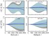 |
Fig. 18 Seasonal consistency of the beams at four HFI frequencies.Thick blue lines show the difference of the Mars season 1 and Mars season 2 window functions normalized to the band-average full window function. The grey shaded band is the ±1σ error for Mars 1 and the blue shaded band is the ±1σ error for Mars 2. |
5.2.2. Time variability of planet flux density
Mars is known to have diurnal variability at HFI frequencies due to the non-uniformity of the surface albedo5. A single detector scans Mars on time scales of a few hours, during which the brightness temperature of Mars can vary by several percent. Additionally, the Mars planetary disc area varies by several percent during an observation as it moves relative to Planck. To assess the impact of Mars variability on the scanning beam determination, GH representations of the beam are derived for each bolometer, with and without a model for the diurnal variability of Mars. Using χ2 tests for goodness of fit, these results are indistinguishable.
5.2.3. Beam colour correction
The scanning beams are measured using planets, whose spectral energy distribution (SED) roughly follows the Rayleigh-Jeans spectrum. However, the beam window functions from these measurements are used to correct the angular power spectra of CMB anisotropies, which is characterized by a very different spectrum, one that is falling in power as a function of frequency relative to a Rayleigh-Jeans spectrum across the HFI bands.
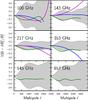 |
Fig. 19 An estimate of known biases in the effective beam window function compared to the RMS statistical error including the additional factor 2.7 (grey shaded region) for each HFI frequency band. Green is the bias due to near sidelobes, blue is the colour-correction bias, and magenta shows an upper limit on the effect of ADC non-linearity. |
Physical optics simulations, using the GRASP6 software, are used to investigate this effect. For each HFI channel from 100–353 GHz, monochromatic simulations are generated at five frequencies across each band using the pre-launch telescope model (Maffei et al. 2010; Tauber et al. 2010). The solid angle of these simulated beams varies across the band, due to diffraction and focussing effects. For 100–217 GHz, the beam size comes to a minimum near the band centre, while at 353 GHz the beam size rises with frequency.
No attempt is made to colour-correct the planet-derived window functions, because a telescope solution has not yet been determined that agrees with the measured solid angles. Spot checks at 143 and 353 GHz with a defocussed telescope model improve agreement between the data and the model, but does not change the trend of solid angle with frequency across the band. The investigation of these effects suggests that numerical models can bound the uncertainty, but cannot reliably predict a bias. Rayleigh-Jeans-weighted average and CMB anisotropy-weighted average beams are produced and used to compute an effective beam window function (blue curves in Fig. 19). The largest bias results at 353 GHz. For the frequencies 100, 143, and 217 GHz, however, the band average effect is less than 0.1% across the entire multipole range used in the CMB likelihood.
The beam solid angle also varies as a function of source SED; the GRASP simulations constrain the size of the beam solid angle colour correction from a ν2 source SED (like the planets) to the IRAS convention ν-1. At 545 and 857 GHz, the GRASP models of Murphy et al. (2010) provide a measure of the effect, which is found to be significant at 353 GHz, but not at the other frequencies, at the level of a few tenths of a percent (Table 2).
5.2.4. ADC non-linearity
Non-linearity in the ADC in the HFI readout electronics mainly manifests itself as an apparent gain drift (Planck Collaboration VI 2014; Planck Collaboration VIII 2014), however, the measured beam shapes are also biased by the effect.
Correcting the ADC non-linearity relies on a model that predicts which ADC codes contribute to each data sample. The presence of large signal gradients, such as a planet, or pickup from the 4He-JT cooler, make modelling difficult. A model for correcting every detector is still under development.
A model of the behaviour of the ADCs is used to apply non-linearity to simulated Mars observations. The B-spline scanning beams reconstructed from these simulations predict biases that are typically under 2% at ℓ ≤ 2000, less than the RMS error (see the magenta curves in Fig. 19 for simulated bias of the 100 through 353 GHz channels).
Using the brighter planets in future Planck main beam models will tend to reduce the effect, as the higher signal amplitudes sample a broader range of the ADC, tending to average down the resulting bias (Mather et al. 1993).
5.2.5. Pointing errors
While the simulated planet observations account for random pointing errors, pointing
drifts remain at the level of a few arcseconds per pointing period in the co-scan and
cross-scan directions common to all detectors (Planck
Collaboration I 2014; Planck Collaboration VI
2014). These have the effect of widening the beam. Even in the worst case, if
remaining errors are Gaussian-distributed with a 2.̋5 residual, the window function
is 0.2% biased at multipole
ℓ = 3000.
Since this is a very small effect relative to the other beam errors, it is considered
negligible.
5.2.6. Glitches
The HFI data are affected by transient signals due to interactions with high energy particles. The planet simulation tools allow for the addition of a random population of glitches to simulated Mars observations with a realistic rate and energy spectrum (Planck Collaboration X 2014), testing the performance of the deglitching algorithm near planet signals and the effects of undetected low energy glitches in the channel with the highest glitch rate at each frequency band.
The RMS of the noise increases by at most 20% in the bolometer with the highest glitch rate, but more typically less than 10%, and the reconstruction bias changes by a negligible amount. The effects are small enough that they are not included in the error budget.
5.3. Relative consistency: window function ratios vs. spectral ratios
The CMB sky itself allows an additional, and statistically powerful, check on the relative consistency (but not the absolute accuracy) of the effective beam window functions within a frequency band. See Fig. 33, and the associated discussion in Sect. 7.3 of Planck Collaboration VI (2014), showing the self-consistency of the window functions at a level better than 0.4%, across the full range of multipoles employed in cosmological parameter estimation.
6. Total error budget
The distribution of beam solid angles reconstructed from simulated planet reconstructions provides the statistical error budget for the beam solid angles (Table 2). Other systematic effects are small in comparison.
The uncertainty in the effective beam window function is determined with the distribution of window functions computed from the simulated beams. These errors are highly correlated in multipole space, and we find that they can be fully described by a small number of eigenmodes and their covariance matrix (Appendices G.1 and G.2), which can be retrieved, together with the nominal beam window functions, from Planck Collaboration (2013) and the Planck Legacy Archive7. These simulations also allow us to determine the bias induced by the beam reconstruction pipeline, and correct the final beam window functions from it (Appendix G.3).
Studies have been performed to probe the impact of assumptions regarding the near sidelobe response of the beam. These studies suggest the potential that the Monte Carlo ensembles used to derive the error eigenmodes may not capture aspects of the bias and the correlation structure of the errors. A visual summary of the total error budget, including the impact of the near sidelobe response, is provided in Fig. 19. For the initial data release a conservative scaling of the MC-derived beam errors, a factor of 2.7 in power, is applied in order to accommodate the maximum extent of the bias that is allowable, given the signal-to-noise ratio of the Jupiter and Saturn data.
7. Conclusion
A combination of Jupiter and Saturn observations, survey difference maps, and checkout and performance verification (CPV) phase data is used to derive the bolometer/readout electronics time response transfer function. This transfer function is deconvolved from the HFI time-ordered data. Residuals can be detected as long tails, stretching up to 6° from compact sources, but are at a level less than 10-4 of the beam peak, and so are insignificant for the scanning beams.
The effective beams and window functions are estimated for all HFI detectors using a scanning beam derived from a combination of the first two seasons of Mars observations. The effective beam products account for the partial symmetrization of the scanning beam which results from the scan strategy. The FEBeCoP algorithm produces effective beams in real space, while the Quickbeam method is used to produce the effective beam window functions and errors in harmonic space.
The final error budget for each effective beam window function (both auto- and cross-beams) is well-described by five eigenmodes for each beam and a correlation matrix of eigenvalues. The error parameters are estimated with an ensemble of simulated Mars observations. The simulations are based on random realizations of noise and pointing errors.
No significant time variation of the scanning beam or the time response is found. Cross-power window functions are also produced that describe the beam filtering effects in cross-correlations between independent HFI maps.
The high signal-to-noise ratio of the Jupiter and Saturn data limit the contribution of the near sidelobe response (between 30′ and 5° of the beam centroid) to the total beam solid angle to less than 0.2% at 100 to 217 GHz. This portion of the beam, which is beyond the signal-to-noise of the Mars data, is not fully represented in the beam simulations. The Monte Carlo derived error amplitudes are scaled by a factor of 2.7 to account for the contribution of the near sidelobe response to the beam window function.
Far sidelobes contribute negligibly to the window function, but may potentially impact the primary calibration and result in pickup from bright Galactic sources. Improved physical optics models for the far sidelobes will be forthcoming for future releases.
The impact of non-linearity in the ADC, the sensitivity of beam shape to the spectral intensity of the source, and residual cosmic ray transients are found to be insignificant sources of systematic error.
Knowledge of the beam window functions allows Planck HFI to extrapolate the dipole calibration over more than three orders of magnitude in angular scale. For the current data release, beam errors are subdominant to noise, foreground marginalization and sample variance in cosmological parameter estimation. Future Planck data releases will fully exploit all of the available planetary data and create wide-field beam maps, allowing an even more precise, and accurate, measurement of the main beams and near sidelobes.
Planck is a project of the European Space Agency – ESA – with instruments provided by two scientific Consortia funded by ESA member states (in particular the lead countries: France and Italy) with contributions from NASA (USA), and telescope reflectors provided in a collaboration between ESA and a scientific Consortium led and funded by Denmark.
The data are convolved with the kernel [ 0.25,0.5,0.25 ] in the time domain.
TICRA, http://www.ticra.com
Acknowledgments
The development of Planck has been supported by: ESA; CNES and CNRS/INSU-IN2P3-INP (France); ASI, CNR, and INAF (Italy); NASA and DoE (USA); STFC and UKSA (UK); CSIC, MICINN, JA and RES (Spain); Tekes, AoF and CSC (Finland); DLR and MPG (Germany); CSA (Canada); DTU Space (Denmark); SER/SSO (Switzerland); RCN (Norway); SFI (Ireland); FCT/MCTES (Portugal); and PRACE (EU). A description of the Planck Collaboration and a list of its members, including the technical or scientific activities in which they have been involved, can be found at http://www.sciops.esa.int/index.php?project=planck&page=Planck_Collaboration.
References
- Armitage-Caplan, C., & Wandelt, B. D. 2009, ApJS, 181, 533 [NASA ADS] [CrossRef] [Google Scholar]
- Cox, M. 1972, J. Instit. Math. Appl., 10, 134 [Google Scholar]
- de Boor, C. 1972, J. Approx. Theor., 6, 50 [CrossRef] [Google Scholar]
- Delabrouille, J., Betoule, M., Melin, J.-B., et al. 2013, A&A, 553, A96 [NASA ADS] [CrossRef] [EDP Sciences] [Google Scholar]
- Dierckx, P. 1993, Curve and Surface Fitting with Splines (Oxford University Press) [Google Scholar]
- Dvorkin, C., & Smith, K. M. 2009, Phys. Rev. D, 79, 043003 [NASA ADS] [CrossRef] [Google Scholar]
- Giorgini, J. D., Yeomans, D. K., Chamberlin, A. B., et al. 1996, in BAAS, 28, 1158 [Google Scholar]
- Górski, K. M., Hivon, E., Banday, A. J., et al. 2005, ApJ, 622, 759 [NASA ADS] [CrossRef] [Google Scholar]
- Hanson, D., Lewis, A., & Challinor, A. 2010, Phys. Rev. D, 81, 103003 [NASA ADS] [CrossRef] [Google Scholar]
- Hill, R. S., Weiland, J. L., Odegard, N., et al. 2009, ApJS, 180, 246 [NASA ADS] [CrossRef] [Google Scholar]
- Hinshaw, G., Nolta, M. R., Bennett, C. L., et al. 2007, ApJS, 170, 288 [NASA ADS] [CrossRef] [Google Scholar]
- Hivon, E., Górski, K. M., Netterfield, C. B., et al. 2002, ApJ, 567, 2 [NASA ADS] [CrossRef] [Google Scholar]
- Holmes, W. A., Bock, J. J., Crill, B. P., et al. 2008, Appl. Opt., 47, 5996 [NASA ADS] [CrossRef] [PubMed] [Google Scholar]
- Hu, W. 2000, Phys. Rev. D, 62, 043007 [NASA ADS] [CrossRef] [Google Scholar]
- Huffenberger, K. M., Crill, B. P., Lange, A. E., Górski, K. M., & Lawrence, C. R. 2010, A&A, 510, A58 [NASA ADS] [CrossRef] [EDP Sciences] [Google Scholar]
- Jarosik, N., Bennett, C. L., Dunkley, J., et al. 2011, ApJS, 192, 14 [NASA ADS] [CrossRef] [Google Scholar]
- Lamarre, J., Puget, J., Ade, P. A. R., et al. 2010, A&A, 520, A9 [NASA ADS] [CrossRef] [EDP Sciences] [Google Scholar]
- Lewis, A., & Challinor, A. 2006, Phys. Rep., 429, 1 [Google Scholar]
- Maffei, B., Noviello, F., Murphy, J. A., et al. 2010, A&A, 520, A12 [NASA ADS] [CrossRef] [EDP Sciences] [Google Scholar]
- Masi, S., Ade, P. A. R., Bock, J. J., et al. 2006, A&A, 458, 687 [NASA ADS] [CrossRef] [EDP Sciences] [Google Scholar]
- Mather, J. C., Fixsen, D. J., & Shafer, R. A. 1993, in SPIE Conf. Ser. 2019, ed. M. S. Scholl, 168 [Google Scholar]
- Mitra, S., Rocha, G., Górski, K. M., et al. 2011, ApJS, 193, 5 [NASA ADS] [CrossRef] [Google Scholar]
- Murphy, J. A., Peacocke, T., Maffei, B., et al. 2010, J. Instrum., 5, 4001 [Google Scholar]
- Nolta, M. R., Dunkley, J., Hill, R. S., et al. 2009, ApJS, 180, 296 [NASA ADS] [CrossRef] [Google Scholar]
- Pajot, F., Ade, P. A. R., Beney, J., et al. 2010, A&A, 520, A10 [NASA ADS] [CrossRef] [EDP Sciences] [Google Scholar]
- Planck Collaboration I. 2011, A&A, 536, A1 [NASA ADS] [CrossRef] [EDP Sciences] [Google Scholar]
- Planck Collaboration VII. 2011, A&A, 536, A7 [NASA ADS] [CrossRef] [EDP Sciences] [Google Scholar]
- Planck Collaboration 2013, The Explanatory Supplement to the Planck 2013 results, http://www.sciops.esa.int/wikiSI/planckpla/index.php?title=Main_Page (ESA) [Google Scholar]
- Planck Collaboration I. 2014, A&A, 571, A1 [NASA ADS] [CrossRef] [EDP Sciences] [Google Scholar]
- Planck Collaboration II. 2014, A&A, 571, A2 [NASA ADS] [CrossRef] [EDP Sciences] [Google Scholar]
- Planck Collaboration III. 2014, A&A, 571, A3 [NASA ADS] [CrossRef] [EDP Sciences] [Google Scholar]
- Planck Collaboration IV. 2014, A&A, 571, A4 [NASA ADS] [CrossRef] [EDP Sciences] [Google Scholar]
- Planck Collaboration V. 2014, A&A, 571, A5 [NASA ADS] [CrossRef] [EDP Sciences] [Google Scholar]
- Planck Collaboration VI. 2014, A&A, 571, A6 [NASA ADS] [CrossRef] [EDP Sciences] [Google Scholar]
- Planck Collaboration VII. 2014, A&A, 571, A7 [NASA ADS] [CrossRef] [EDP Sciences] [Google Scholar]
- Planck Collaboration VIII. 2014, A&A, 571, A8 [NASA ADS] [CrossRef] [EDP Sciences] [Google Scholar]
- Planck Collaboration IX. 2014, A&A, 571, A9 [NASA ADS] [CrossRef] [EDP Sciences] [Google Scholar]
- Planck Collaboration X. 2014, A&A, 571, A10 [NASA ADS] [CrossRef] [EDP Sciences] [Google Scholar]
- Planck Collaboration XI. 2014, A&A, 571, A11 [NASA ADS] [CrossRef] [EDP Sciences] [Google Scholar]
- Planck Collaboration XII. 2014, A&A, 571, A12 [NASA ADS] [CrossRef] [EDP Sciences] [Google Scholar]
- Planck Collaboration XIII. 2014, A&A, 571, A13 [NASA ADS] [CrossRef] [EDP Sciences] [Google Scholar]
- Planck Collaboration XIV. 2014, A&A, 571, A14 [NASA ADS] [CrossRef] [EDP Sciences] [Google Scholar]
- Planck Collaboration XV. 2014, A&A, 571, A15 [NASA ADS] [CrossRef] [EDP Sciences] [Google Scholar]
- Planck Collaboration XVI. 2014, A&A, 571, A16 [NASA ADS] [CrossRef] [EDP Sciences] [Google Scholar]
- Planck Collaboration XVII. 2014, A&A, 571, A17 [NASA ADS] [CrossRef] [EDP Sciences] [Google Scholar]
- Planck Collaboration XVIII. 2014, A&A, 571, A18 [NASA ADS] [CrossRef] [EDP Sciences] [Google Scholar]
- Planck Collaboration XIX. 2014, A&A, 571, A19 [NASA ADS] [CrossRef] [EDP Sciences] [Google Scholar]
- Planck Collaboration XX. 2014, A&A, 571, A20 [NASA ADS] [CrossRef] [EDP Sciences] [Google Scholar]
- Planck Collaboration XXI. 2014, A&A, 571, A21 [NASA ADS] [CrossRef] [EDP Sciences] [Google Scholar]
- Planck Collaboration XXII. 2014, A&A, 571, A22 [NASA ADS] [CrossRef] [EDP Sciences] [Google Scholar]
- Planck Collaboration XXIII. 2014, A&A, 571, A23 [NASA ADS] [CrossRef] [EDP Sciences] [MathSciNet] [PubMed] [Google Scholar]
- Planck Collaboration XXIV. 2014, A&A, 571, A24 [NASA ADS] [CrossRef] [EDP Sciences] [Google Scholar]
- Planck Collaboration XXV. 2014, A&A, 571, A25 [NASA ADS] [CrossRef] [EDP Sciences] [Google Scholar]
- Planck Collaboration XXVI. 2014, A&A, 571, A26 [NASA ADS] [CrossRef] [EDP Sciences] [Google Scholar]
- Planck Collaboration XXVII. 2014, A&A, 571, A27 [NASA ADS] [CrossRef] [EDP Sciences] [Google Scholar]
- Planck Collaboration XXVIII. 2014, A&A, 571, A28 [NASA ADS] [CrossRef] [EDP Sciences] [Google Scholar]
- Planck Collaboration XXIX. 2014, A&A, 571, A29 [NASA ADS] [CrossRef] [EDP Sciences] [Google Scholar]
- Planck Collaboration XXX. 2014, A&A, 571, A30 [NASA ADS] [CrossRef] [EDP Sciences] [Google Scholar]
- Planck Collaboration XXXI. 2014, A&A, 571, A31 [NASA ADS] [CrossRef] [EDP Sciences] [Google Scholar]
- Planck HFI Core Team. 2011a, A&A, 536, A4 [NASA ADS] [CrossRef] [EDP Sciences] [Google Scholar]
- Planck HFI Core Team. 2011b, A&A, 536, A6 [NASA ADS] [CrossRef] [EDP Sciences] [Google Scholar]
- Prezeau, G., & Reinecke, M. 2010, ApJS, 190, 267 [NASA ADS] [CrossRef] [Google Scholar]
- Reinecke, M., Dolag, K., Hell, R., Bartelmann, M., & Enßlin, T. A. 2006, A&A, 445, 373 [NASA ADS] [CrossRef] [EDP Sciences] [Google Scholar]
- Ruze, J. 1966, IEEE Proc., 54, 633 [Google Scholar]
- Sallen, R. P., & Key, E. L. 1955, Circuit Theory, IRE Trans., 2, 74 [Google Scholar]
- Tauber, J. A., Norgaard-Nielsen, H. U., Ade, P. A. R., et al. 2010, A&A, 520, A2 [NASA ADS] [CrossRef] [EDP Sciences] [Google Scholar]
- Tristram, M., Filliard, C., Perdereau, O., et al. 2011, A&A, 534, A88 [NASA ADS] [CrossRef] [EDP Sciences] [Google Scholar]
- Tristram, M., Patanchon, G., Macías-Pérez, J. F., et al. 2005, A&A, 436, 785 [NASA ADS] [CrossRef] [EDP Sciences] [Google Scholar]
- Wandelt, B. D., & Gorski, K. M. 2001, Phys. Rev. D, 63, 123002 [NASA ADS] [CrossRef] [Google Scholar]
- Weiland, J. L., Odegard, N., Hill, R. S., et al. 2011, ApJS, 192, 19 [Google Scholar]
Appendix A: Electronics model
HFI electronics filter sequence; here s = iω.
Parameters for LFER4 model that are deconvolved from the data.
This Appendix derives the effect of the HFI electronics filtering on the TOI. If the
input signal (power) on a bolometer is  (A.1)the bolometer physical impedance can be
written as:
(A.1)the bolometer physical impedance can be
written as:  (A.2)where ω is the angular frequency
of the signal and F(ω) is the complex intrinsic
bolometer transfer function. For HFI the bolometer transfer function is modelled as the
sum of 4 single pole low pass filters,
(A.2)where ω is the angular frequency
of the signal and F(ω) is the complex intrinsic
bolometer transfer function. For HFI the bolometer transfer function is modelled as the
sum of 4 single pole low pass filters,  (A.3)The modulation of the signal is done with a
square wave, written here as a composition of sine waves of decreasing amplitude,
(A.3)The modulation of the signal is done with a
square wave, written here as a composition of sine waves of decreasing amplitude,
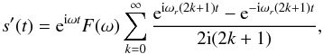 (A.4)where the Euler relation sinx =
(eix−e−ix)
/2i is used, and ωr is the angular
frequency of the square wave. The modulation frequency is fmod =
ωr/2π
and was set to fmod
= 90.18759 Hz in flight. This signal is then filtered by the complex
electronic transfer function H(ω). Setting
(A.4)where the Euler relation sinx =
(eix−e−ix)
/2i is used, and ωr is the angular
frequency of the square wave. The modulation frequency is fmod =
ωr/2π
and was set to fmod
= 90.18759 Hz in flight. This signal is then filtered by the complex
electronic transfer function H(ω). Setting
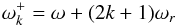 and
and 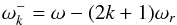 gives
gives ![Mathematical equation: \appendix \setcounter{section}{1} \begin{equation} \label{sigele} \Sigma(t)=\sum_{k=0}^\infty\frac{F(\omega)}{2{\rm i}(2k+1)}\left[H(\omega_k^+){\rm e}^{{\rm i}\omega_k^+t}-H(\omega_k^-){\rm e}^{{\rm i}\omega_k^-t}\right]. \end{equation}](/articles/aa/full_html/2014/11/aa21535-13/aa21535-13-eq209.png) (A.5)This signal is then sampled at high frequency
(2fmodNsamp).
Nsamp is a parameter of the HFI
electronics corresponding to the number of high frequency samples in each modulation
semi-period. In order to obtain an output signal sampled every π/ωr
seconds, the waveform is integrated on a semi-period, as done in the HFI readout. To also
include a time shift Δt, the integral is calculated between
nπ/ωr +
Δt and (n +
1)π/ωr +
Δt (with T =
2π/ωr
period of the modulation). The time shift Δt is encoded in the HFI electronics by the
parameter Sphase, with the relation Δt =
Sphase/Nsamp/fmod.
(A.5)This signal is then sampled at high frequency
(2fmodNsamp).
Nsamp is a parameter of the HFI
electronics corresponding to the number of high frequency samples in each modulation
semi-period. In order to obtain an output signal sampled every π/ωr
seconds, the waveform is integrated on a semi-period, as done in the HFI readout. To also
include a time shift Δt, the integral is calculated between
nπ/ωr +
Δt and (n +
1)π/ωr +
Δt (with T =
2π/ωr
period of the modulation). The time shift Δt is encoded in the HFI electronics by the
parameter Sphase, with the relation Δt =
Sphase/Nsamp/fmod.
After integration, a sample of a bolometer at time tn can be written as
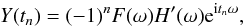 (A.6)where
 ![Mathematical equation: \appendix \setcounter{section}{1} \begin{eqnarray} \label{tfele} H'(\omega) = \frac 12 \sum_{k=0}^\infty {\rm e}^{-{\rm i}(\frac{\pi\omega}{2\omega_r}+\omega\Delta t)} \Bigg[ \frac{H(\omega_k^+){\rm e}^{{\rm i}\omega_k^+ \Delta t}}{(2k+1)\omega_k^+} \left(1-{\rm e}^{\frac{{\rm i}\omega_k^+\pi}{\omega_r}}\right) &&\nonumber\\ - \frac{H(\omega_k^-){\rm e}^{{\rm i}\omega_k^- \Delta t}}{(2k+1)\omega_k^-} \left(1-{\rm e}^{\frac{{\rm i}\omega_k^-\pi}{\omega_r}}\right)&& \Bigg]. \end{eqnarray}](/articles/aa/full_html/2014/11/aa21535-13/aa21535-13-eq220.png) (A.7)The output signal in Eq. (A.6) can be demodulated (thus removing the
(−
1)n) and compared to the input signal in
Eq. (A.1). The overall transfer function
is composed of the bolometer transfer function and the effective electronics transfer
function, H′(ω),
(A.7)The output signal in Eq. (A.6) can be demodulated (thus removing the
(−
1)n) and compared to the input signal in
Eq. (A.1). The overall transfer function
is composed of the bolometer transfer function and the effective electronics transfer
function, H′(ω),
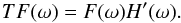 (A.8)The shape of H(ω) is
obtained by combining low and high-pass filters with Sallen Key topologies (Sallen & Key 1955), with their respective time
constants, and accounting also for the stray capacitance low pass filter given by the
bolometer impedance combined with the stray capacitance of the cables. The sequence of
filters that define the electronic band-pass function H(ω) =
h0 ∗ h1 ∗
h2 ∗ h3 ∗
h4 ∗ h5 are
listed in Table A.1, with parameters listed in
Table A.2.
(A.8)The shape of H(ω) is
obtained by combining low and high-pass filters with Sallen Key topologies (Sallen & Key 1955), with their respective time
constants, and accounting also for the stray capacitance low pass filter given by the
bolometer impedance combined with the stray capacitance of the cables. The sequence of
filters that define the electronic band-pass function H(ω) =
h0 ∗ h1 ∗
h2 ∗ h3 ∗
h4 ∗ h5 are
listed in Table A.1, with parameters listed in
Table A.2.
Appendix B: Gauss-Hermite beams
HFI’s scanning beams are described by an elliptical Gaussian shape to an accuracy of 2–5% in solid angle. A Gauss-Hermite representation of the beam uses Hermite polynomials to provide higher-order corrections to a Gaussian model (Huffenberger et al. 2010). There are fewer degrees of freedom than in a gridded beam map, allowing higher signal-to-noise on each mode. However, because the order of the decomposition is truncated, in practice the description is ill suited to a description of features much beyond the extent of the main beam. Larger scale features of the beam, including a beam shoulder (Ruze 1966) or the effect of the print-through of the backing structure (grating lobes), must be included separately.
The initial two-dimensional Gaussian is parametrized as ![Mathematical equation: \appendix \setcounter{section}{2} \begin{equation} \label{eq:2dGaussian} P(x_1,x_2) = \frac{A}{|2\pi\vec{\Sigma}|^{1/2}}\exp\left[-\frac12\sum_{i,j=1}^{2}(x_i-{\bar x}_i)\Sigma^{-1}_{ij}(x_j-{\bar x}_j)\right], \end{equation}](/articles/aa/full_html/2014/11/aa21535-13/aa21535-13-eq225.png) (B.1)where A is an overall amplitude,
(x1,x2) are
two-dimensional Cartesian coordinates (the pointing is projected to a flat sky),
(B.1)where A is an overall amplitude,
(x1,x2) are
two-dimensional Cartesian coordinates (the pointing is projected to a flat sky),
 are the coordinates of the beam centre, and the correlation matrix is given by
 (B.2)Hence, the Gaussian model parameters
 are fitted. These can also be expressed in terms of the ellipticity, e (defined here as the
ratio between the major and minor axes), and rotation angle α, of the Gaussian ellipse.
are fitted. These can also be expressed in terms of the ellipticity, e (defined here as the
ratio between the major and minor axes), and rotation angle α, of the Gaussian ellipse.
The coefficients to the Gauss-Hermite polynomials multiplying the elliptical Gaussian are
then fitted. The basis functions are defined as
 (B.3)where Hn(x)
is the order-n Hermite polynomial and the primed coordinates
x′ rotates
into a system aligned with the axes of the Gaussian and scaled to the major and minor axes
σi (i.e., to the
principle axes of the correlation matrix Σ). Having determined the elliptical Gaussian
separately, the subsequent Gauss-Hermite polynomial fit is a generalized least-squares
procedure, solvable by the usual matrix techniques, under the assumption of white noise.
Because the full data model includes further effects such as pointing error, glitch
effects, etc, a full error analysis requires a broad suite of simulations, described in
Sect. 5.
(B.3)where Hn(x)
is the order-n Hermite polynomial and the primed coordinates
x′ rotates
into a system aligned with the axes of the Gaussian and scaled to the major and minor axes
σi (i.e., to the
principle axes of the correlation matrix Σ). Having determined the elliptical Gaussian
separately, the subsequent Gauss-Hermite polynomial fit is a generalized least-squares
procedure, solvable by the usual matrix techniques, under the assumption of white noise.
Because the full data model includes further effects such as pointing error, glitch
effects, etc, a full error analysis requires a broad suite of simulations, described in
Sect. 5.
Appendix C: B-spline beams
In this model of the scanning beam, a two-dimensional B-spline surface is fit to the time-ordered planet data. A smoothing criterion is applied during the fit to minimize the effects of high spatial frequency variations due to noise. This representation of the beam is superior to a simple two-dimensional binning of the data in its ability to capture large signal gradients.
B-splines are a linear combination of polynomials of degree k and order k + 1. They are defined by the location of their control points (called knots) of which there are 5 for 3rd degree polynomials.
The k-degree
B-spline
built using the knots {λi,...,λi
+ k + 1} (de
Boor 1972; Cox 1972) is given by
![Mathematical equation: \appendix \setcounter{section}{3} \begin{equation} P_{i,1}(x) = \left\{ \begin{array}{l} 1, \mbox{ if } x \in \mbox{[} \lambda_{i}, \lambda_{i+1} \mbox{]}\\ 0, \mbox{ if } x \notin \mbox{[} \lambda_{i}, \lambda_{i+1} \mbox{]} \end{array} \right. \end{equation}](/articles/aa/full_html/2014/11/aa21535-13/aa21535-13-eq241.png) (C.1)with recursion relations
(C.1)with recursion relations
 (C.2)where the index l runs from 1 through the
B-spline
degree k. The
B-spline
knots {λi,...,zλi
+ k + 1} are located on a regularly spaced
grid in the detector coordinate frame. At the edge of the reconstructed beam map area, 4
coincident knots are added to avoid vanishing basis functions, allowing a unique
decomposition.
(C.2)where the index l runs from 1 through the
B-spline
degree k. The
B-spline
knots {λi,...,zλi
+ k + 1} are located on a regularly spaced
grid in the detector coordinate frame. At the edge of the reconstructed beam map area, 4
coincident knots are added to avoid vanishing basis functions, allowing a unique
decomposition.
In the solution to the B-spline coefficients Pi,l(x), a smoothing criterion is introduced as a constraint on the sum of the derivatives of the beam at each knot, motivated by the assumption that the true beam does not contain very high spatial frequencies and prevents noise from biasing the reconstruction at spatial frequencies smaller than the smoothing scale.
A smoothing criterion η (Dierckx
1993) is related to the sum of the order k derivative of the beam model (Pk) evaluated at the knot
locations λi: ![Mathematical equation: \appendix \setcounter{section}{3} \begin{equation} \eta = \displaystyle{\sum_{i=1}^{g}\left[P^{k}(\lambda_{i+})-P^{k}(\lambda_{i-})\right]^2} \label{eq:smoothcrit} \end{equation}](/articles/aa/full_html/2014/11/aa21535-13/aa21535-13-eq248.png) (C.3)where g is the total number of
distinct knots and λi + and
λi
− are the left and right derivative of the beam model evaluated
at the knot location. The smoothing criterion is introduced as an extra term in the score
function ζ in
the least-squares minimization of the beam map with respect to the data,
(C.3)where g is the total number of
distinct knots and λi + and
λi
− are the left and right derivative of the beam model evaluated
at the knot location. The smoothing criterion is introduced as an extra term in the score
function ζ in
the least-squares minimization of the beam map with respect to the data,
 (C.4)where δ is the usual squared
difference between the data points yr and the model
P(xr)
at pointings xr,
(C.4)where δ is the usual squared
difference between the data points yr and the model
P(xr)
at pointings xr,
![Mathematical equation: \appendix \setcounter{section}{3} \begin{equation} \delta = \displaystyle{\sum_{r=1}^{m}}\left[y_{r} - P(x_{r})\right]^2. \end{equation}](/articles/aa/full_html/2014/11/aa21535-13/aa21535-13-eq258.png) (C.5)and p is a relative weighting
factor for the smoothing criterion. The knot spacing and the smoothing criterion weight
p are
determined separately for each frequency band based on physical optics simulations and the
coverage of the two Mars transits given by the scanning strategy (see Table C.1). Simulated planet observations (see Sect. 5) show that the choice of B-spline knot spacing and
smoothing parameters do not significantly bias the beam reconstruction.
(C.5)and p is a relative weighting
factor for the smoothing criterion. The knot spacing and the smoothing criterion weight
p are
determined separately for each frequency band based on physical optics simulations and the
coverage of the two Mars transits given by the scanning strategy (see Table C.1). Simulated planet observations (see Sect. 5) show that the choice of B-spline knot spacing and
smoothing parameters do not significantly bias the beam reconstruction.
Summary of B-spline knot spacing and smoothing criterion weight p used in the beam reconstruction.
Appendix D: Far sidelobe effects on the effective beam window function
The far sidelobes (FSL) are defined as the response of the instrument at angles >5° from the main beam centroid. The FSL affect both 1. the gain calibration of the instrument with the dipole, and 2. how the calibration is transfered to higher multipoles with the effective beam window function. Here we discuss the interplay of these effects.
The FSL can be separated into three main components (see Fig. 5 of Tauber et al. 2010):
-
1.
Primary Reflector Spillover (PR Spillover) is the response ofthe instrument to radiation from just above the primary mirror thatreflects off the secondary mirror and arrives at the feed horns. Thisresponse is nearly aligned with the spin axis of the spacecraft, andtherefore scans very little of the sky on 1 min time-scales.
-
2.
Secondary Reflector Direct Spillover(SR Direct Spillover, or SRD) is the response from directly above the secondary mirror. The sidelobe peaks roughly 10° from the main beam, and as such scans the sky in nearly the same way as the main beam as the satellite rotates. The azimuthal extent is roughly 30°.
-
3.
Secondary Reflector Baffle Spillover (SR Baffle Spillover, or SRB) is response from radiation reflecting off the baffles. This is difficult to model, being diffuse radiation reflecting off the poorly known inner baffle surfaces. It is spread over a large fraction of the sky.
The HFI dipole calibration is performed assuming a delta-function (pencil) beam (Planck Collaboration VIII 2014). This leads to a bias
in the calibration described by the ratio of the dipole convolved with the full-sky beam
to the dipole convolved by a pencil beam, 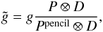 where
where  is the estimated gain, g is the true gain,
P is the
true full-sky beam, Ppencil is the assumed pencil beam, and
D is the
dipole. The true full-sky beam is taken to consist of three portions,
is the estimated gain, g is the true gain,
P is the
true full-sky beam, Ppencil is the assumed pencil beam, and
D is the
dipole. The true full-sky beam is taken to consist of three portions,
 the main beam Pmain (within
20′ of the centroid), the
near sidelobes PNSL (between 20′ and 5°), and the far sidelobes PFSL (response
further than 5° from the
centroid). The quantity
the main beam Pmain (within
20′ of the centroid), the
near sidelobes PNSL (between 20′ and 5°), and the far sidelobes PFSL (response
further than 5° from the
centroid). The quantity  is defined as the beam within
5° of the centroid (the
main lobe and near sidelobes). The bias in the calibration can be rewritten as
is defined as the beam within
5° of the centroid (the
main lobe and near sidelobes). The bias in the calibration can be rewritten as
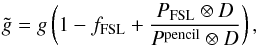 (D.1)where fFSL is the
integral of the far sidelobe response relative to the full beam integral. The first term,
1 −
fFSL, is due to the loss in response of the
main lobe and near sidelobes to far sidelobes, while the second term represents the
coupling of the dipole into the sidelobes.
(D.1)where fFSL is the
integral of the far sidelobe response relative to the full beam integral. The first term,
1 −
fFSL, is due to the loss in response of the
main lobe and near sidelobes to far sidelobes, while the second term represents the
coupling of the dipole into the sidelobes.
For each pointing period the convolution of the pencil beam with the dipole is
approximated by  (D.2)where θmain is the
angle between the main beam centroid and the spin axis, and dpencil is the
dipole amplitude that would be observed with a pencil beam. The components of the far
sidelobes enter into Eq. (D.1)
differently, and assuming the majority of the response to the dipole in each component
comes from one direction on the sky, can be approximated as
(D.2)where θmain is the
angle between the main beam centroid and the spin axis, and dpencil is the
dipole amplitude that would be observed with a pencil beam. The components of the far
sidelobes enter into Eq. (D.1)
differently, and assuming the majority of the response to the dipole in each component
comes from one direction on the sky, can be approximated as
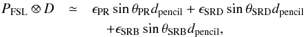 where ϵPR,
ϵSRD, and ϵSRB are the
fraction of the total solid angle in the PR spillover, the SR direct spillover, and the SR
baffle spillover, respectively, and θPR, θSRD,
θSRB are the angles between the spin axis
and the peak of the PR spillover response, the SR direct spillover response, and the SR
baffle spillover response respectively. Equation (D.1) then simplifies to
where ϵPR,
ϵSRD, and ϵSRB are the
fraction of the total solid angle in the PR spillover, the SR direct spillover, and the SR
baffle spillover, respectively, and θPR, θSRD,
θSRB are the angles between the spin axis
and the peak of the PR spillover response, the SR direct spillover response, and the SR
baffle spillover response respectively. Equation (D.1) then simplifies to 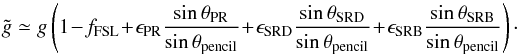 (D.3)From Tauber
et al. (2010), θpencil ≃ 85°, θPR ≃ 10°,
θSRD ≃
75°, and θSRB ≃ 45° making the PR spillover and
SR baffle spillover negligible. Equation (D.3) reduces further to
(D.3)From Tauber
et al. (2010), θpencil ≃ 85°, θPR ≃ 10°,
θSRD ≃
75°, and θSRB ≃ 45° making the PR spillover and
SR baffle spillover negligible. Equation (D.3) reduces further to 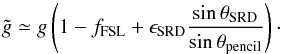 (D.4)SR direct spillover scans the dipole, but
with a slightly different amplitude, since it is offset by 10° from the main lobe. The PR spillover
does not modulate the dipole; aligned with the spin axis, the PR spillover contributes a
nearly constant signal during each stable pointing period. The predicted values of the
solid angle fractions are fFSL = 3.3 × 10⁻³ and
ϵSRD = 1.9 ×
10-3 at 100 GHz (Tauber et
al. 2010), making the measured gain
(D.4)SR direct spillover scans the dipole, but
with a slightly different amplitude, since it is offset by 10° from the main lobe. The PR spillover
does not modulate the dipole; aligned with the spin axis, the PR spillover contributes a
nearly constant signal during each stable pointing period. The predicted values of the
solid angle fractions are fFSL = 3.3 × 10⁻³ and
ϵSRD = 1.9 ×
10-3 at 100 GHz (Tauber et
al. 2010), making the measured gain  .
.
However, the effect of the gain bias on the angular power spectrum is further reduced by
corrections to the effective beam window function due to the FSL. Not including the FSL in
the beam model tends to bias the window function at very low multipoles relative to high
multipoles. Considering the measured sky signal at small scales
 as compared to the true sky
Tsky one has
as compared to the true sky
Tsky one has
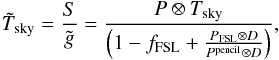 where S is the signal measured by
the bolometer. Solving for the true sky signal gives
where S is the signal measured by
the bolometer. Solving for the true sky signal gives  Considering that PMNSL ⊗
Tsky ≃ (1 −
fFSL)Tsky,
Considering that PMNSL ⊗
Tsky ≃ (1 −
fFSL)Tsky,
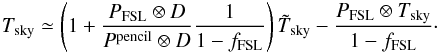 Now also considering that PMNSL ⊗ D ≃ (1 −
fFSL)Ppencil ⊗
D, the true sky signal can be written as
Now also considering that PMNSL ⊗ D ≃ (1 −
fFSL)Ppencil ⊗
D, the true sky signal can be written as
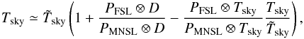 or
or  (D.5)where the second-order correction term
 is dropped, and the following factors are
defined:
is dropped, and the following factors are
defined:  and
and  Here φsky represents
the relative pickup of anisotropy in the sidelobe beam as compared to the main beam and
near sidelobes. The response of the FSL to CMB anisotropy is negligible, but Galactic
response may not be. The PR spillover contributes only a constant value per pointing
period, because it is not modulated with the scan. Only the SR direct spillover enters
into the formula. Since the SR direct spillover is nearly aligned with the main beam,
Galactic signal is not picked up in the CMB anisotropy except close to the Galactic plane.
So for foreground-clean regions of the sky, φsky ≪ fFSL.
Here φsky represents
the relative pickup of anisotropy in the sidelobe beam as compared to the main beam and
near sidelobes. The response of the FSL to CMB anisotropy is negligible, but Galactic
response may not be. The PR spillover contributes only a constant value per pointing
period, because it is not modulated with the scan. Only the SR direct spillover enters
into the formula. Since the SR direct spillover is nearly aligned with the main beam,
Galactic signal is not picked up in the CMB anisotropy except close to the Galactic plane.
So for foreground-clean regions of the sky, φsky ≪ fFSL.
The quantity φD is the bias due to
the ratio of dipole response in the far sidelobes to dipole response in the main beam.
Again the PR spillover contributes only an offset per pointing period, which is removed by
the polkapix destriping algorithm (Tristram et al. 2011; Planck Collaboration VIII
2014), so we are left with the SR direct spillover and SR baffle spillover.
Applying the same approximation as in Eq. (D.2) gives  and Eq. (D.5) becomes
  (D.6)This result implies that FSL bias of the
effective beam window function tends to cancel the gain bias (Eq. (D.4)), and the response to CMB anisotropy is
unaffected to first order.
(D.6)This result implies that FSL bias of the
effective beam window function tends to cancel the gain bias (Eq. (D.4)), and the response to CMB anisotropy is
unaffected to first order.
Simulations of the sky scanned with the far sidelobe physical optics model (Planck Collaboration XIV 2014; Planck Collaboration VI 2014) confirm this.
Appendix E: Harmonic space computation of the effective beam window function
Two harmonic space techniques (FICSBell and Quickbeam), developed independently but closely related in their formalism, have been used to compute the effective beam window functions. They provide a valuable cross-check of the pixel-based results obtained with FEBeCoP (Fig. 2) and their low computational requirements allow fast calculation of the window function errors through the processing of Monte Carlo simulations of planet observations.
Appendix E.1: FICSBell
FICSBell is a harmonic space method for computing the effective beam window function directly from the scanning beam and the scan history. The steps of this method are as follows.
-
1.
The statistics of the orientation of each detec-tor d within each map pixel p is computed first, andonly once for a given observation campaign:
 (E.1)where ψj is the
orientation of the detector with respect to the local meridian during the
measurement j occurring in the direction rp.
Note that the s =
0 moment is simply the hit count map. The orientation hit
moments are computed up to degree s = 4. At the same time, the first two
moments of the distribution of samples within each pixel (i.e., the centre of mass
and moments of inertia) are computed and stored.
(E.1)where ψj is the
orientation of the detector with respect to the local meridian during the
measurement j occurring in the direction rp.
Note that the s =
0 moment is simply the hit count map. The orientation hit
moments are computed up to degree s = 4. At the same time, the first two
moments of the distribution of samples within each pixel (i.e., the centre of mass
and moments of inertia) are computed and stored. -
2.
The scanning beam map of each detector d is transformed into spherical harmonics:
 (E.2)where Bd(r)
is the beam map centred on the north pole, and the Yℓs(r)
are the spherical harmonic basis functions. Higher s indices describe
higher degrees of departure from azimuthal symmetry and, for HFI beams, the
coefficients
(E.2)where Bd(r)
is the beam map centred on the north pole, and the Yℓs(r)
are the spherical harmonic basis functions. Higher s indices describe
higher degrees of departure from azimuthal symmetry and, for HFI beams, the
coefficients  are decreasing functions of
s
at most multipoles considered. It also appears that, for ℓ< 3000, the
coefficients with |s
| > 4 account for much less than 1% of the beam solid angle.
Spot checks where window functions are computed with |s| ≤ 6 show a
difference of less than 10-4 for ℓ< 2000 at 100 GHz and for
ℓ<
3000 at 143 and 217 GHz. For these reasons, only modes with
|s| ≤
4 are considered in the present analysis. Armitage-Caplan & Wandelt (2009) reached a similar
conclusion in their deconvolution of LFI beams.
are decreasing functions of
s
at most multipoles considered. It also appears that, for ℓ< 3000, the
coefficients with |s
| > 4 account for much less than 1% of the beam solid angle.
Spot checks where window functions are computed with |s| ≤ 6 show a
difference of less than 10-4 for ℓ< 2000 at 100 GHz and for
ℓ<
3000 at 143 and 217 GHz. For these reasons, only modes with
|s| ≤
4 are considered in the present analysis. Armitage-Caplan & Wandelt (2009) reached a similar
conclusion in their deconvolution of LFI beams. -
3.
For a given CMB sky realization t, described by its spherical harmonics coefficients aℓm = ∫drt(r)Yℓm(r), the
coefficients computed above are
used to generate s-spin weighted maps,
 (E.3)as well as the first and second
derivatives, using standard HEALPix tools.
(E.3)as well as the first and second
derivatives, using standard HEALPix tools. -
4.
The spin-weighted maps and orientation hit moments of the same order s are combined for all detectors involved, to provide an “observed” map
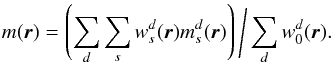 (E.4)Similarly the local spatial
derivatives are combined with the location hit moments to describe the effect of
the non-ideal sampling of each pixel (see Appendix F). In this combination, the respective number of hits of each detector
in each pixel is considered, as well as the detector weighting (generally
proportional to the inverse noise variance).
(E.4)Similarly the local spatial
derivatives are combined with the location hit moments to describe the effect of
the non-ideal sampling of each pixel (see Appendix F). In this combination, the respective number of hits of each detector
in each pixel is considered, as well as the detector weighting (generally
proportional to the inverse noise variance). -
5.
The power spectrum of this map can then be computed, and compared to the input CMB power spectrum to estimate the effective beam window function over the whole sky, or over a given region of the sky.
Monte Carlo (MC) simulations in which the sky realizations are changed can be performed by repeating steps 3, 4 and 5. The impact of beam model uncertainties can be studied by including step 2 in the MC simulations.
Appendix E.2: Quickbeam
By decomposing the scanning beam into harmonic coefficients Bℓm, each TOI sample
can be modelled as (neglecting the contribution from instrumental noise, which is
independent of beam asymmetry) 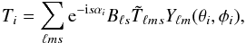 (E.5)where the TOI samples are indexed by
i, and
(E.5)where the TOI samples are indexed by
i, and
 is the underlying sky signal. The spin
spherical harmonic
is the underlying sky signal. The spin
spherical harmonic  rotates the scanning beam to the
pointing location (θ,φ), while the e−
isαi
factor gives it the correct orientation. Equation (E.5)may be evaluated using techniques developed for convolution in
Wandelt & Gorski (2001) and Prezeau & Reinecke (2010), although manipulating
a TOI-sized object is necessarily slow.
rotates the scanning beam to the
pointing location (θ,φ), while the e−
isαi
factor gives it the correct orientation. Equation (E.5)may be evaluated using techniques developed for convolution in
Wandelt & Gorski (2001) and Prezeau & Reinecke (2010), although manipulating
a TOI-sized object is necessarily slow.
On the small angular scales comparable to the size of the beam, it is a good
approximation to assume that the procedure of mapmaking from TOI samples is essentially
a process of binning: 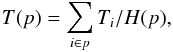 (E.6)where H(p) is
the total number of hits in pixel
(E.6)where H(p) is
the total number of hits in pixel  .
.
Given a normalized, rescaled harmonic transform of the beam Bℓm, sky multipoles
and a scan history object
 given by
 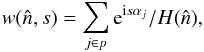 (E.7)where the sum is over all hits
j of
pixel p at
location
(E.7)where the sum is over all hits
j of
pixel p at
location  ,
and αj is the scan angle
for observation j. The harmonic transform of this scan-strategy
object is given by
,
and αj is the scan angle
for observation j. The harmonic transform of this scan-strategy
object is given by 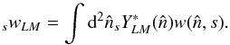 (E.8)The beam-convolved observation is then
given by
(E.8)The beam-convolved observation is then
given by 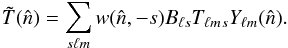 (E.9)Taking the ensemble average of the
pseudo-Cℓ power spectrum
of these Tlm gives (Hanson et al. 2010; Hinshaw et al. 2007)
(E.9)Taking the ensemble average of the
pseudo-Cℓ power spectrum
of these Tlm gives (Hanson et al. 2010; Hinshaw et al. 2007)
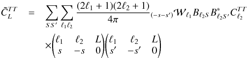 (E.10)where
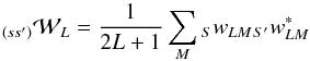 (E.11)is a cross-power spectrum of scan history
objects. Note that the w(n,s) used here can also
incorporate a position dependent weighting to optimize the pseudo-Cℓ estimate, such as
inverse-noise or a mask, the equations are unchanged. Writing the pseudo-Cℓ in position space
(following Dvorkin & Smith 2009) with Wigner-d
matrices gives
(E.11)is a cross-power spectrum of scan history
objects. Note that the w(n,s) used here can also
incorporate a position dependent weighting to optimize the pseudo-Cℓ estimate, such as
inverse-noise or a mask, the equations are unchanged. Writing the pseudo-Cℓ in position space
(following Dvorkin & Smith 2009) with Wigner-d
matrices gives ![Mathematical equation: \appendix \setcounter{section}{5} \begin{eqnarray} \tilde{C}_{L}^{{TT}} &=& \frac{1}{8\pi} \sum_{S S'} \int_{-1}^{1} {\rm d}z \ d^{L}_{00}(z) \nonumber\\&&\quad \times \left[\sum_{\ell_1} d^{\ell_1}_{-s -s'}(z) {}_{(-s -s')}{\cal W}_{\ell_1} (2\ell_1+1) \right] \nonumber\\&&\quad \times \left[ \sum_{\ell_2} d^{\ell_2}_{s s'}(z) B_{\ell_2 S} B_{\ell_2 S'}^* C^{{TT}}_{\ell_2}(2\ell_2+1) \right]. \end{eqnarray}](/articles/aa/full_html/2014/11/aa21535-13/aa21535-13-eq350.png) (E.12)This integral can be implemented exactly
using Gauss-Legendre quadrature, at a cost of
(E.12)This integral can be implemented exactly
using Gauss-Legendre quadrature, at a cost of  . For simplicity, the equations here are
written for the auto-spectrum of a single detector, but the generalization to a map made
by adding several detectors with different weightings is straightforward. The cost to
compute all of the necessary terms exactly in that case becomes
. For simplicity, the equations here are
written for the auto-spectrum of a single detector, but the generalization to a map made
by adding several detectors with different weightings is straightforward. The cost to
compute all of the necessary terms exactly in that case becomes
 .
.
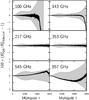 |
Fig. E.1 Difference between effective beam window functions computed with a real space method (FEBeCoP) and a harmonic space method (Quickbeam). The shaded region denotes the RMS error at each mutipole. |
On the flat sky, beam convolution is multiplication in Fourier space by a beam rotated onto the scan direction. Multiple hits with different scan directions are incorporated by averaging (as the scan history objects above encapsulate).
A scan strategy which is fairly smooth across the sky is nearly equivalent to observing
many independent flat-sky patches at high L. There is a fairly good approximation to the
beam convolved pseudo-power spectrum which is essentially a flat-sky approximation. In
the limit that L ≫
ℓ1, with Cℓ2 and
Bℓ2 is a
slowly-varying function in ℓ2, and using the equality
 (E.13)the pseudo-Cℓ sum above can be
approximated as
(E.13)the pseudo-Cℓ sum above can be
approximated as  (E.14)where the average ⟨⟩p is taken
over the full sky. It is illustrative to consider two limits of this equation. Firstly,
for a “raster” scan strategy in which each pixel is observed with the same
direction:
(E.14)where the average ⟨⟩p is taken
over the full sky. It is illustrative to consider two limits of this equation. Firstly,
for a “raster” scan strategy in which each pixel is observed with the same
direction: (E.15)and the predicted transfer function is just
the power spectrum of the beam. Secondly, for a “best-case” scan strategy, in which each
pixel is observed many times with many different orientation angles,
(E.15)and the predicted transfer function is just
the power spectrum of the beam. Secondly, for a “best-case” scan strategy, in which each
pixel is observed many times with many different orientation angles,
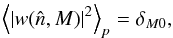 (E.16)and the transfer function is the
azimuthally symmetric part of the beam. Note that this is for a full-sky observation; in
the presence of a mask, the average above produces an fsky factor,
as expected but neglects the coupling between L multipoles (which can be calculated with the
more complete equations above).
(E.16)and the transfer function is the
azimuthally symmetric part of the beam. Note that this is for a full-sky observation; in
the presence of a mask, the average above produces an fsky factor,
as expected but neglects the coupling between L multipoles (which can be calculated with the
more complete equations above).
Appendix F: Pixelization artefacts
PlanckHFI maps are produced at HEALPix resolution 11 (Nside = 2048), corresponding to pixels with a typical dimension of 1.́7. With the resolution comparable to the spacing between scanning rings (Planck Collaboration I 2011) there is an uneven distribution of hits within pixels, introducing a complication in the analysis and interpretation of the Planck maps. A sample of the Planck distribution of sample hits within pixels is illustrated in Fig. F.
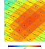 |
Fig. F.1 Illustration of TOI samples near the Galactic plane (grey dots), over-plotted on a simulated CMB realization which has been convolved with a Gaussian 7′ FWHM beam and pixelized at (Nside = 2048). Associated scanning rings (grey lines) as well as centres of mass for the hit distribution (black arrows) are also plotted. |
The three effective beam codes may also be used to simulate the effect of pixelization on the observed sky: LevelS/TotalConvoler/Conviqt (Reinecke et al. 2006; Wandelt & Gorski 2001; Prezeau & Reinecke 2010); FEBeCoP (Mitra et al. 2011; and FICSBell (Appendix E).
For the measurement of CMB fluctuations, the effects of pixelization may be studied
analytically. On the small scales relevant to pixelization, the observed CMB is smooth,
both due to physical damping and the convolution of the instrumental beam. Taylor
expanding the CMB temperature about a pixel centre to second order, the typical gradient
amplitude is given by 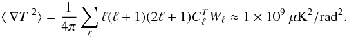 (F.1)Here the approximate value is calculated for
a ΛCDM cosmology with a
7′ FWHM Gaussian beam. The
typical curvature of the observed temperature, on the other hand is given by
(F.1)Here the approximate value is calculated for
a ΛCDM cosmology with a
7′ FWHM Gaussian beam. The
typical curvature of the observed temperature, on the other hand is given by
![Mathematical equation: \appendix \setcounter{section}{6} \begin{equation} \langle|\nabla^2 T|^2 \rangle = \frac{1}{4\pi} \sum_{\ell} [\ell(\ell+1)]^2(2\ell+1) C_\ell^{T} W_\ell \approx 7\times10^{14} ~\mu K^2/{\rm rad}^4. \end{equation}](/articles/aa/full_html/2014/11/aa21535-13/aa21535-13-eq367.png) (F.2)On the scales relevant to the maximum
displacement from the centre of a 1.7′ pixel, the maximum displacement is of order 1′(3 × 10⁻⁴rad)), and so the gradient term tends to dominate,
although the curvature term is still non-negligible. For each observation of a pixel, the
displacement from the pixel centre can be denoted as d =
dθ +
idφ. The average over
all hits within a pixel gives an overall deflection vector for a pixel centre located at
denoted as
(F.2)On the scales relevant to the maximum
displacement from the centre of a 1.7′ pixel, the maximum displacement is of order 1′(3 × 10⁻⁴rad)), and so the gradient term tends to dominate,
although the curvature term is still non-negligible. For each observation of a pixel, the
displacement from the pixel centre can be denoted as d =
dθ +
idφ. The average over
all hits within a pixel gives an overall deflection vector for a pixel centre located at
denoted as  .
This represents the centre of mass of the hit distribution; Fig. F shows these average deflections using black arrows. The deflection
field
may be decomposed into spin-1 spherical harmonics as
.
This represents the centre of mass of the hit distribution; Fig. F shows these average deflections using black arrows. The deflection
field
may be decomposed into spin-1 spherical harmonics as
 (F.3)With a second-order Taylor expansion of the
CMB temperature about each pixel centre, it is then possible to calculate the average
pseudo-Cℓ power spectrum of
the pixelized sky. This is given by
(F.3)With a second-order Taylor expansion of the
CMB temperature about each pixel centre, it is then possible to calculate the average
pseudo-Cℓ power spectrum of
the pixelized sky. This is given by ![Mathematical equation: \appendix \setcounter{section}{6} \begin{eqnarray} C_\ell^{T} = \left[1-\ell(\ell+1)R^d\right] {C}_\ell^{T} W_\ell + \frac{1}{2} \sum_{\ell_1 \ell_2} \frac{\ell_1(\ell_1+1)(2\ell_1+1)(2\ell_2+1)}{4\pi} &&\nonumber\\ \times \threej{\ell_1}{\ell_2}{\ell}{1}{-1}{0}^2 C_{\ell_1}^{T} W_{\ell_1} \left[ C_{\ell_2}^{d+} + (-1)^{\ell + \ell_1 + \ell_2} C_{\ell_2}^{ d-} \right],&& \label{eqn:clt_pixelized} \end{eqnarray}](/articles/aa/full_html/2014/11/aa21535-13/aa21535-13-eq373.png) (F.4)where Rd = ⟨|d|2 ⟩ /2 is half the mean-squared
deflection magnitude (averaged over hits within a pixel, as well as over pixels),
(F.4)where Rd = ⟨|d|2 ⟩ /2 is half the mean-squared
deflection magnitude (averaged over hits within a pixel, as well as over pixels),
 is the sum of the gradient and curl power
spectra of dℓm, and
is the sum of the gradient and curl power
spectra of dℓm, and
 is the gradient spectrum minus the curl
spectrum. The Rd term describes a
smearing of the observed sky due to pixelization. For uniform pixel coverage of
Nside =
2048 pixels ⟨|d|2 ⟩ 1/2 =
(2Rd)1/2 =
0.725′, while, for the hit distribution of Planck
frequency maps, Rd is within 0.2% of
this value for CMB channels, and 0.4% for all channels. This term is therefore accurately
described by the HEALPix pixel window function, which is derived
under the assumption of uniform pixel coverage, and the resulting relative error on the
beam window function is at most 4 ×
10-4 for ℓ ≤ 3000.
is the gradient spectrum minus the curl
spectrum. The Rd term describes a
smearing of the observed sky due to pixelization. For uniform pixel coverage of
Nside =
2048 pixels ⟨|d|2 ⟩ 1/2 =
(2Rd)1/2 =
0.725′, while, for the hit distribution of Planck
frequency maps, Rd is within 0.2% of
this value for CMB channels, and 0.4% for all channels. This term is therefore accurately
described by the HEALPix pixel window function, which is derived
under the assumption of uniform pixel coverage, and the resulting relative error on the
beam window function is at most 4 ×
10-4 for ℓ ≤ 3000.
The effect of pixelization is degenerate with that of gravitational lensing of the CMB, with the difference that it: (1) acts on the beam-convolved sky, rather than the actual sky; and (2) produces a curl-mode deflection field as well as a gradient mode. This is discussed further in Planck Collaboration XVII (2014), where the sub-pixel deflection field constitutes a potential source of bias for the measured Planck lensing potential. Indeed, Eq. (F.4) is just a slightly modified version of the usual first order CMB lensing power spectrum (Hu 2000), Lewis & Challinor (2006) to accommodate curl modes.
A useful approximation to Eq. (F.4) which
is derived in the unrealistic limit that the deflection vectors are uncorrelated between
pixels, but in practice gives a good description of the power induced by the pixelization,
is that the
couples the CMB gradient into a source of noise with an effective level given by
 (F.5)where the average is taken over all pixels
and RT is half the mean-squared power in the
CMB gradient:
(F.5)where the average is taken over all pixels
and RT is half the mean-squared power in the
CMB gradient:  (F.6)For frequency-combined maps,
 is typically on the order of 0.́1, and so
the induced noise σN is approximately
2 μK′. This
is small compared to the instrumental contribution, although it does not disappear when
taking cross-spectra, depending on the coherence of the hit distributions of the two maps
in the cross-spectra.
is typically on the order of 0.́1, and so
the induced noise σN is approximately
2 μK′. This
is small compared to the instrumental contribution, although it does not disappear when
taking cross-spectra, depending on the coherence of the hit distributions of the two maps
in the cross-spectra.
Appendix G: Beam window function error
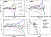 |
Fig. G.1 Beam window function error modes. Panels a), b) and
c) show the first six eigenmodes defined in Eq. (G.11) for respectively the effective
auto-beam 100ds1 and 143ds2 and the effective cross-beam 217-1 × 217-2. The first five modes used in
the current beam error modelling are shown as solid coloured curves, while the 6th
mode (the first one to be ignored) appears as yellow dashes. The grey dashes show
the ±1 σ envelope obtained
by adding the first five modes in quadrature, while the solid grey curve is the
±1 σ envelope estimated
from the simulations (therefore including all eigenmodes). The black dashes show the
relative difference between |

Appendix G.1: Error eigenmodes
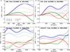 |
Fig. G.2 Effect of ℓ truncation on beam error modes for frequency-averaged beam window functions at 100, 143, 217 GHz and 143 × 217. For clarity, only the three leading modes are shown, respectively, in blue, green and red, while the solid grey line shows the 1 σ level, obtained by adding all modes in quadrature. Dotted lines are the original eigenmodes computed on a wide ℓ-range. Solid lines are the eigenmodes computed directly from the MC simulations on the truncated ℓ-range used for cosmological analysis. Dashed lines show the eigenmodes computed on the truncated ℓ-range with Eqs. (G.16) and (G.17), starting from the first five eigenmodes for the wide range. In all four cases considered, the first leading mode on the truncated range, which dominates the error budget, is perfectly reconstructed out of the information available, while the second leading mode is well estimated in all cases except for 217 GHz. |
Consider two individual detectors or detection units (weighted sum of detectors)
X and
Y for
which sky maps are available. Here X and Y can be the same or different. Putting aside the
instrumental noise and other contingencies for the time being, the cross- (or auto-)
angular power spectrum measured of the observed maps
 is on average related
to the real input signal
is on average related
to the real input signal  through
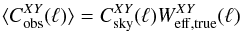 (G.1)where
 is the effective beam window function.
Note that because of the optical beam non-circularity and Planck
scanning strategy,
is the effective beam window function.
Note that because of the optical beam non-circularity and Planck
scanning strategy, ![Mathematical equation: \appendix \setcounter{section}{7} \begin{equation} W^{XY}(\ell) \ne \left[W^{XX}(\ell) W^{YY}(\ell)\right]^{1/2} \quad\text{if}\ X \ne Y, \end{equation}](/articles/aa/full_html/2014/11/aa21535-13/aa21535-13-eq402.png) (G.2)as illustrated in Fig. 16, while WXY =
WYX for any
X and
Y. It
also appears that in the ℓ range of interest, WXY(ℓ) ≥
0; therefore
(G.2)as illustrated in Fig. 16, while WXY =
WYX for any
X and
Y. It
also appears that in the ℓ range of interest, WXY(ℓ) ≥
0; therefore  , analogous to what is usually done for
simple (circular) beam models. In what follows, the XY pair superscript is
dropped except when they are required for clarity. In most cases, scientific analyses
will be conducted on a best guess Cest(ℓ) of the sky
power spectrum, in which the empirical Cobs(ℓ) is corrected
from a nominal effective window Weff,nom(ℓ)
, analogous to what is usually done for
simple (circular) beam models. In what follows, the XY pair superscript is
dropped except when they are required for clarity. In most cases, scientific analyses
will be conducted on a best guess Cest(ℓ) of the sky
power spectrum, in which the empirical Cobs(ℓ) is corrected
from a nominal effective window Weff,nom(ℓ) (G.3)therefore, on average,
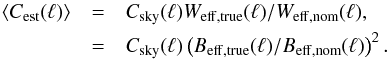 (G.4)The ratio Beff,true(ℓ)
/Beff,nom(ℓ) which
determines the uncertainties on the angular power spectrum originating from our beam
knowledge is studied using the planet transit MC simulations described in Sect. 5. The scanning beam map determined with the
B-Spline
code described in Appendix C on each of these
simulations is turned into an effective beam window function Wi(ℓ)
for i =
1,2,...,nMC (where
nMC =
100 is the number of MC simulations) using the Quickbeam
formalism described in Appendix E.2.
(G.4)The ratio Beff,true(ℓ)
/Beff,nom(ℓ) which
determines the uncertainties on the angular power spectrum originating from our beam
knowledge is studied using the planet transit MC simulations described in Sect. 5. The scanning beam map determined with the
B-Spline
code described in Appendix C on each of these
simulations is turned into an effective beam window function Wi(ℓ)
for i =
1,2,...,nMC (where
nMC =
100 is the number of MC simulations) using the Quickbeam
formalism described in Appendix E.2.
Defining the means Bmean(ℓ) and
Wmean(ℓ) as
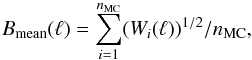 (G.5)and,
  (G.6)one can build the matrix of the deviations
around the mean
(G.6)one can build the matrix of the deviations
around the mean  (G.7)where the factor fs has been applied. As
discussed in Sect. 6, fs =
2.7. This scaling factor is applied throughout the rest of discussion
and is included in the delivered products and plotted error modes.
(G.7)where the factor fs has been applied. As
discussed in Sect. 6, fs =
2.7. This scaling factor is applied throughout the rest of discussion
and is included in the delivered products and plotted error modes.
Sect. G.3 contains a discussion of how the MC average Bmean and nominal beam Beff,nom are related and focus here on the dispersion around the mean.
Since the relative dispersion of the simulated Wi(ℓ)
generally is very small (less than 1%), then Wmean(ℓ) ≃
Bmean(ℓ)2
to a very good approximation (as illustrated in Fig. G.1) and the matrix Δ is well approximated by
![Mathematical equation: \appendix \setcounter{section}{7} \begin{eqnarray} \Delta_i(\ell) &\simeq& 1/2 \ \bsfudge \ln\left[W_i(\ell)/\Wmean(\ell)\right], \nonumber \\ \ &\simeq& 1/2 \ \bsfudge \left[W_i(\ell)/\Wmean(\ell) - 1\right]. \end{eqnarray}](/articles/aa/full_html/2014/11/aa21535-13/aa21535-13-eq424.png) (G.8)The quantity B(ℓ) was
preferred over W(ℓ) in order to remain
consistent with the usual description of the beam in linear map space, instead of
quadratic space.
(G.8)The quantity B(ℓ) was
preferred over W(ℓ) in order to remain
consistent with the usual description of the beam in linear map space, instead of
quadratic space.
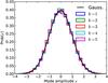 |
Fig. G.3 Distribution of the eigenmodes determined from MC simulations, for all HFI detector sets, for the first nmodes = 5 modes, compared to a Gaussian distribution of zero mean and unit variance. |
The statistical properties of the MC based beam window functions can be summarized in
the covariance of the deviations Δ, defined as 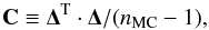 (G.9)where Δ is a matrix with
nMC rows and ℓmax + 1
columns, and C
is a square symmetric positive semi-definite matrix with ℓmax + 1 rows
and columns. It can be diagonalized into
(G.9)where Δ is a matrix with
nMC rows and ℓmax + 1
columns, and C
is a square symmetric positive semi-definite matrix with ℓmax + 1 rows
and columns. It can be diagonalized into 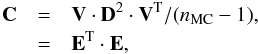 (G.10)where D is a diagonal matrix, with
at most nMC positive eigenvalues, and the
eigenmodes matrix
(G.10)where D is a diagonal matrix, with
at most nMC positive eigenvalues, and the
eigenmodes matrix  (G.11)of the beam uncertainty. Alternatively, one
can perform a singular value decomposition (SVD) of Δ, which reads
(G.11)of the beam uncertainty. Alternatively, one
can perform a singular value decomposition (SVD) of Δ, which reads  where M is an orthogonal
nMC ×
nMC matrix (i.e., MT·M = M·MT =
InMC),
D is a
diagonal matrix with nMC non-negative eigenvalues of
decreasing amplitude, and V is a matrix with ℓmax + 1 rows
whose nMC columns are orthonormal vectors
(i.e., VTV =
InMC), with
InMC being
the identity matrix of size nMC × nMC.
The diagonalization of the covariance matrix C (Eq. (G.10)) has a numerical complexity scaling like
where M is an orthogonal
nMC ×
nMC matrix (i.e., MT·M = M·MT =
InMC),
D is a
diagonal matrix with nMC non-negative eigenvalues of
decreasing amplitude, and V is a matrix with ℓmax + 1 rows
whose nMC columns are orthonormal vectors
(i.e., VTV =
InMC), with
InMC being
the identity matrix of size nMC × nMC.
The diagonalization of the covariance matrix C (Eq. (G.10)) has a numerical complexity scaling like
 , while the SVD of Δ (Eq. (G.12)) scales like
 . Since nMC ≪
ℓmax the latter approach was prefered
because it is much faster, and it naturally provides the mixing matrix M. Equation (G.12) has a degeneracy on the sign of
M and
V, which was
lifted by constraining the vectors of V (and therefore E) to all be positive at
ℓ = 200.
. Since nMC ≪
ℓmax the latter approach was prefered
because it is much faster, and it naturally provides the mixing matrix M. Equation (G.12) has a degeneracy on the sign of
M and
V, which was
lifted by constraining the vectors of V (and therefore E) to all be positive at
ℓ = 200.
It appears that most of the statistical content of Δ or C is described by the first few modes nmodes with the largest eigenvalues, in which case the E matrix is truncated to its first nmodes rows with little loss of information. For HFI, nmodes = 5 is chosen, as illustrated in Fig. G.1.
The statistics of the elements of the mixing matrix M, and therefore of the MC measured beam window function fluctuations, is shown in Fig. G.3 to be very close to Gaussian, justifying the current analysis in terms of a covariance matrix.
The beam uncertainty model therefore is 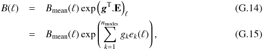 where g is a nmodes element
vector of independant Gaussian variates of zero mean and unit variance and
ek(ℓ)
is the kth
row of E.
where g is a nmodes element
vector of independant Gaussian variates of zero mean and unit variance and
ek(ℓ)
is the kth
row of E.
The SVD decomposition of the beam uncertainty was performed for the ℓ range [ ℓmin,ℓmax ] with ℓmin = 0 and ℓmax depending on the frequencies of the two detectors involved in the beam considered. Currently ℓmax = 2500 when the lowest frequency is 100 GHz, ℓmax = 3000 when that frequency is 143 GHz, and ℓmax = 4000 at higher frequency.
If orthogonal error eigenmodes are needed for the range
![Mathematical equation: \hbox{$[\lmin',\lmax']$}](/articles/aa/full_html/2014/11/aa21535-13/aa21535-13-eq456.png) , with
, with  and
and  , the provided E must first be truncated to
the new range to give the Et matrix with
nmodes rows and
, the provided E must first be truncated to
the new range to give the Et matrix with
nmodes rows and
 columns, and then singular value
decomposed into
columns, and then singular value
decomposed into  (G.16)where the new set of orthogonal eigenmodes is
 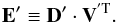 (G.17)This is illustrated in Fig. G.2,
where the eigenmodes are truncated to the frequency dependent ℓ ranges used in the
PlanckC(ℓ) likelihood (Planck Collaboration XV 2014).
(G.17)This is illustrated in Fig. G.2,
where the eigenmodes are truncated to the frequency dependent ℓ ranges used in the
PlanckC(ℓ) likelihood (Planck Collaboration XV 2014).
Appendix G.2: Eigenmode covariance
The previous approach, dedicated to the study of the uncertainty on the beam window
function associated with a single pair of detectors (or maps), can be generalized to the
simultaneous characterization of any number of pairs. For instance, for the three
disjoint pairs, a = {
UV }, b = { XY } and c = { ZT
}, one writes
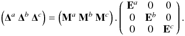 (G.18)and the covariance matrix reads
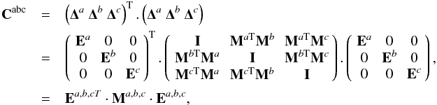 (G.19)where Ma,b,c is a square
symmetric matrix with 3nmodes rows, and if one denotes
La,b,c its Cholesky
“root,” such that Ma,b,c =
La,b,c·La,b,cT,
then
(G.19)where Ma,b,c is a square
symmetric matrix with 3nmodes rows, and if one denotes
La,b,c its Cholesky
“root,” such that Ma,b,c =
La,b,c·La,b,cT,
then 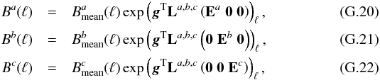 where g is the
3nmodes element vector of independent
Gaussian deviates and is the same for Eqs. (G.20) to (G.22).
where g is the
3nmodes element vector of independent
Gaussian deviates and is the same for Eqs. (G.20) to (G.22).
The Planck-HFI Reduced Instrument Model (RIMO) available at Planck Legacy Archive8 and described in Planck Collaboration (2013) contains the correlation matrix Ma,b,c,d,..., where a,b,c,d... each are a different element of the set of pairs that can be built out of the detection units available. So, for nd detection units, the number of pairs will be nd(nd + 1)/2 and the correlation matrix will be square and symmetric, with the value “1” on its diagonal and have nmodesnd(nd + 1)/2 rows and as many columns. The nmodes relative to the same detector pair form adjacent rows and columns in the matrix, and the order of appearance of the pairs in the matrix is specified in the header of the FITS extension containing the matrix. The nominal Bℓ and eigenmodes E are provided for each pair in a different extension.
The results above were obtained in the basis of eigenmodes provided, if one wants to
obtain a beam correlated model on a different ℓ-range, with the eigenmodes E′ defined in Eq. (G.17), then the covariance matrix becomes
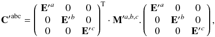 (G.23)with
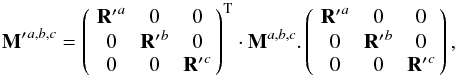 (G.24)where the R′ matrices are obtained from
the SVD in Eq. (G.16).
(G.24)where the R′ matrices are obtained from
the SVD in Eq. (G.16).
Appendix G.3: Monte Carlo bias
As discussed in Sect. 3.2, the Monte Carlo
average of the B-Spline reconstructed effective beam window
function Bmean(ℓ) can be
different from the effective beam that would be obtained directly out of the simulation
input beam map Beff,in(ℓ),
introduces a bias  (G.25)which is interpreted as a consequence of
the imperfect sampling of the beam map by the planet, the effect of the instrumental
noise and pointing uncertainty and the smoothing feature of the B-spline functions. It is
found that |εbias(ℓ = 500)| ≤ 2 ×
10-4 and |εbias(ℓ = 1000)| < 5 ×
10-4 for all effective beams, making it smaller than the
relative dispersion on the beam window function described above. It is assumed that the
beam reconstruction on the real data suffers from the same bias, and its beam window
function Beff,raw(ℓ) is
corrected for this to provide the nominal beam
(G.25)which is interpreted as a consequence of
the imperfect sampling of the beam map by the planet, the effect of the instrumental
noise and pointing uncertainty and the smoothing feature of the B-spline functions. It is
found that |εbias(ℓ = 500)| ≤ 2 ×
10-4 and |εbias(ℓ = 1000)| < 5 ×
10-4 for all effective beams, making it smaller than the
relative dispersion on the beam window function described above. It is assumed that the
beam reconstruction on the real data suffers from the same bias, and its beam window
function Beff,raw(ℓ) is
corrected for this to provide the nominal beam ![Mathematical equation: \appendix \setcounter{section}{7} \begin{eqnarray} B_{\rm eff, nom}(\ell) &=& B_{\rm eff, raw}(\ell) \,/\, \left[1 + \bias(\ell)\right], \\ \ &=& B_{\rm eff, raw}(\ell)\, B_{\rm eff, in}(\ell) \,/\, \Bmean(\ell). \end{eqnarray}](/articles/aa/full_html/2014/11/aa21535-13/aa21535-13-eq490.png) In doing so, εbias is
assumed to be perfectly determined by the simulations, and no error is associated with
this correction.
In doing so, εbias is
assumed to be perfectly determined by the simulations, and no error is associated with
this correction.
All Tables
Observation seasons of the planets observed by Planck: date range and position in Galactic coordinates.
Scanning beam solid angle (ΩSB) error budget, showing the bias and fractional error due to the residual time response (ΔΩτ), near sidelobes (ΔΩNSL) and solid angle colour correction (ΔΩCC).
Summary of B-spline knot spacing and smoothing criterion weight p used in the beam reconstruction.
All Figures
|
Fig. 1 Data flow for fitting time response model parameters. |
| In the text | |
|
Fig. 2 Data flow for determining the HFI beams. |
| In the text | |
|
Fig. 3 Survey 2 minus Survey 1 residual close to the Galactic centre before (upper) and after (lower) fitting and deconvolving the low frequency part of the time response for bolometer 353-2. Remaining residuals are dominated by gain difference between the surveys due to ADC non-linearity (Planck Collaboration VIII 2014) and artifacts of the different scanning directions (beam asymmetry) and pixel coverage survey to survey. |
| In the text | |
|
Fig. 4 68%, 95%, and 99% likelihood contours for the long time constant τ3 and associated amplitude a3 for a 545 GHz bolometer (545-4) with (black) and without (red) zodiacal emission and far sidelobe removal. The square and cross indicate the maximum likelihood values. |
| In the text | |
|
Fig. 5 Survey 1 minus survey 2 residual for the 545 GHz bolometers, averaged from Galactic longitude 0 through 20°. The black curves show the Planck data, and red is a simulation. |
| In the text | |
|
Fig. 6 Gridded Jupiter data for bolometer 143-3b before and after fitting for LFER4 parameters. The best fit Gaussian is subtracted from each plot to emphasize residuals. Residuals in the main beam show the deviation from a Gaussian shape, captured in the representations of the scanning beam, as described in Appendices B and C. |
| In the text | |
|
Fig. 7 Phase and amplitude as a function of signal frequency of the deconvolution function of bolometer 217-1. The solid black curve is the LFER4 model, while the dashed red curve shows the TF10 model used in the earlier Planck papers. The vertical dotted line marks the signal frequency corresponding to the half power point of the average effective beam. |
| In the text | |
|
Fig. 8 Window functions of the planetary discs of Jupiter, Saturn, and Mars, equivalent to the bias in the inferred effective beam window function if the beam is reconstructed from observations of one of these planets alone. The labels show the corresponding angular radius of each disc. |
| In the text | |
|
Fig. 9 B-spline scanning beams reconstructed from Mars, Saturn, and Jupiter seasons 1, 2 and 3 data for near sidelobe studies. The beams are plotted in logarithmic contours of − 3, − 10, − 20 and − 30 dB from the peak. PSB pairs are indicated with the a bolometer in black and the b bolometer in blue. |
| In the text | |
|
Fig. 10 Azimuthally- and band-averaged main beam profiles (black solid curve) derived from the B-spline representation of the first and second Mars observations compared to that derived from a combination of Mars, Jupiter and Saturn observations (filled and open markers represent positive and negative data respectively). The red dashed line is defined as the joint envelope of the main beam and near sidelobe dataset, the integral of which represents the maximal solid angle that is compatible with these data. A nominal near lobe model, provided as a reasonable extrapolation of the data below the noise floor, is shown as the blue dashed line. The fractional increase in solid angle, relative to the Mars-alone derived beam profile, is displayed in each panel. The black dotted line shows the GRASP physical optics model averaged over a subset of detectors that have been simulated (100–353 GHz). The data show a clear excess in power over the model at 143, 217 and 353 GHz that is consistent with a spectrum of surface errors on scales between 2 and 12 cm, with an RMS of order 10 μm. Table 2 contains an estimate of the fraction of the solid angle in the near sidelobes that is not captured in the B-spline representation. For clarity, the figure extends only to 45′. In all cases the solid angle is derived from the profile extending out to 5°. Due to the high signal-to-noise of the Jupiter data (− 40 to − 55 dB, depending on the frequency), and the rapidly falling response of the beam, the solid angle estimates are insensitive to the limit of integration. |
| In the text | |
|
Fig. 11 One scanning beam at each HFI frequency (100-3b, 143-6, 217-1, 353-7, 545-1, and 857-3). Contours are in dB from the peak in steps of −5 dB. The lowest contours are set at −30 dB, −35 dB, −40 dB, −45 dB, −45 dB, −45 dB at 100 GHz, 143 GHz, 217 GHz, 353 GHz, 545 GHz, and 857 GHz, respectively. |
| In the text | |
|
Fig. 12 Gridded data from all five seasons of Jupiter. The colour scale shows the absolute value of the peak signal. |
| In the text | |
|
Fig. 13 A slice through stacked Jupiter data for bolometer 143-6, illustrating residual long time response after deconvolution. The vertical dotted line shows the extent of the scanning beam map (plotted in blue). |
| In the text | |
|
Fig. 14 Azimuthally averaged profiles of measured beams of channel 353-1 compared to the azimuthal average of the far sidelobe physical optics model. |
| In the text | |
|
Fig. 15 Effective beam solid angle (upper panel) and the best-fit Gaussian ellipticity (lower panel) of the 100 GHz effective beam across the sky in Galactic coordinates. |
| In the text | |
|
Fig. 16 Ratios of the cross-beam window functions |
| In the text | |
|
Fig. 17 Effective beam window functions (solid lines) for each HFI frequency. The shaded region shows the ± 1σ error envelope. Dashed lines show the effective beam window function for Gaussian beams with FWHM 9.́65, 7.́25, 4.́99, 4.́82, 4.́68, and 4.́33 for 100, 143, 217, 353, 545 and 857 GHz, respectively. |
| In the text | |
|
Fig. 18 Seasonal consistency of the beams at four HFI frequencies.Thick blue lines show the difference of the Mars season 1 and Mars season 2 window functions normalized to the band-average full window function. The grey shaded band is the ±1σ error for Mars 1 and the blue shaded band is the ±1σ error for Mars 2. |
| In the text | |
|
Fig. 19 An estimate of known biases in the effective beam window function compared to the RMS statistical error including the additional factor 2.7 (grey shaded region) for each HFI frequency band. Green is the bias due to near sidelobes, blue is the colour-correction bias, and magenta shows an upper limit on the effect of ADC non-linearity. |
| In the text | |
|
Fig. E.1 Difference between effective beam window functions computed with a real space method (FEBeCoP) and a harmonic space method (Quickbeam). The shaded region denotes the RMS error at each mutipole. |
| In the text | |
|
Fig. F.1 Illustration of TOI samples near the Galactic plane (grey dots), over-plotted on a simulated CMB realization which has been convolved with a Gaussian 7′ FWHM beam and pixelized at (Nside = 2048). Associated scanning rings (grey lines) as well as centres of mass for the hit distribution (black arrows) are also plotted. |
| In the text | |
|
Fig. G.1 Beam window function error modes. Panels a), b) and
c) show the first six eigenmodes defined in Eq. (G.11) for respectively the effective
auto-beam 100ds1 and 143ds2 and the effective cross-beam 217-1 × 217-2. The first five modes used in
the current beam error modelling are shown as solid coloured curves, while the 6th
mode (the first one to be ignored) appears as yellow dashes. The grey dashes show
the ±1 σ envelope obtained
by adding the first five modes in quadrature, while the solid grey curve is the
±1 σ envelope estimated
from the simulations (therefore including all eigenmodes). The black dashes show the
relative difference between |
| In the text | |
|
Fig. G.2 Effect of ℓ truncation on beam error modes for frequency-averaged beam window functions at 100, 143, 217 GHz and 143 × 217. For clarity, only the three leading modes are shown, respectively, in blue, green and red, while the solid grey line shows the 1 σ level, obtained by adding all modes in quadrature. Dotted lines are the original eigenmodes computed on a wide ℓ-range. Solid lines are the eigenmodes computed directly from the MC simulations on the truncated ℓ-range used for cosmological analysis. Dashed lines show the eigenmodes computed on the truncated ℓ-range with Eqs. (G.16) and (G.17), starting from the first five eigenmodes for the wide range. In all four cases considered, the first leading mode on the truncated range, which dominates the error budget, is perfectly reconstructed out of the information available, while the second leading mode is well estimated in all cases except for 217 GHz. |
| In the text | |
|
Fig. G.3 Distribution of the eigenmodes determined from MC simulations, for all HFI detector sets, for the first nmodes = 5 modes, compared to a Gaussian distribution of zero mean and unit variance. |
| In the text | |
Current usage metrics show cumulative count of Article Views (full-text article views including HTML views, PDF and ePub downloads, according to the available data) and Abstracts Views on Vision4Press platform.
Data correspond to usage on the plateform after 2015. The current usage metrics is available 48-96 hours after online publication and is updated daily on week days.
Initial download of the metrics may take a while.