| Issue |
A&A
Volume 699, July 2025
|
|
|---|---|---|
| Article Number | A183 | |
| Number of page(s) | 34 | |
| Section | Extragalactic astronomy | |
| DOI | https://doi.org/10.1051/0004-6361/202553897 | |
| Published online | 08 July 2025 | |
Spatially resolved spectrophotometric SED modeling of NGC 253’s central molecular zone
I. Star formation in extragalactic giant molecular clouds
1
Departamento de Astronomia, Instituto de Astronomia, Geofísica e Ciências Atmosféricas da USP, Cidade Universitária, 05508-090 São Paulo, SP, Brazil
2
Astronomical Observatory of the Jagiellonian University, Orla 171, 30-244 Kraków, Poland
3
National Center for Nuclear Research, ul. Pasteura 7, 02-093 Warsaw, Poland
4
Scuola Internazionale Superiore di Studi Avanzati (SISSA), Via Bonomea 265, IT-34136 Trieste, Italy
5
Institute for Fundamental Physics of the Universe (IFPU), Via Beirut 2, IT-34151 Trieste, Italy
6
INAF – Osservatorio di Astrofisica e Scienza dello Spazio (OAS), Via Gobetti 93/3, I-40127 Bologna, Italy
7
ICSC – Centro Nazionale di Ricerca in High Performance Computing, Big Data e Quantum Computing, Via Magnanelli 2, Bologna, Italy
8
Universidade Federal de Santa Catarina, Campus Universitário Reitor João David Ferreira Lima, 88040-900 Florianópolis, SC, Brazil
9
European Southern Observatory, Alonso de Córdova, 3107, Vitacura, Santiago 763-0355, Chile
10
Joint ALMA Observatory, Alonso de Córdova, 3107, Vitacura Santiago 763-0355, Chile
11
Centro de Estudios de Física del Cosmos de Aragón (CEFCA), Plaza San Juan 1, E–44001 Teruel, Spain
12
Centro de Astrobiología (CAB), CSIC-INTA, Carretera de Ajalvir km 4, Torrejón de Ardoz, 28850 Madrid, Spain
13
National Radio Astronomy Observatory, 520 Edgemont Road, Charlottesville, VA 22903-2475, USA
14
Max-Planck-Institut für Radioastronomie, Auf-dem-Hügel 69, 53121 Bonn, Germany
15
Xinjiang Astronomical Observatory, Chinese Academy of Sciences, 830011 Urumqi, China
16
National Astronomical Observatory of Japan, 2-21-1 Osawa, Mitaka, Tokyo 181-8588, Japan
17
Institute of Astronomy and Astrophysics, Academia Sinica, 11F of AS/NTU Astronomy-Mathematics Building, No.1, Sec. 4, Roosevelt Rd, Taipei 106319, Taiwan
18
Department of Astronomy, School of Science, The Graduate University for Advanced Studies (SOKENDAI), 2-21-1 Osawa, Mitaka, Tokyo 181-1855, Japan
19
Institute of Astrophysics, Facultad de Ciencias Exactas, Universidad Andrés Bello, Sede Concepción, Talcahuano, Chile
20
New Mexico Institute of Mining and Technology, 801 Leroy Place, Socorro, NM 87801, USA
21
International Gemini Observatory/NSF NOIRLab, Casilla 603, La Serena, Chile
22
Instituto de Astrofísica de La Plata, CONICET-UNLP, Paseo del Bosque s/n, La Plata B1900FWA, Argentina
23
Department of Space, Earth and Environment, Chalmers University of Technology, Onsala Space Observatory, SE-43992 Onsala, Sweden
24
Department of Physics, Faculty of Science and Technology, Keio University, 3-14-1 Hiyoshi, Yokohama, Kanagawa 223–8522, Japan
25
Institute of Astronomy, Graduate School of Science, The University of Tokyo, 2-21-1 Osawa, Mitaka, Tokyo 181-0015, Japan
26
NOAO, 950 North Cherry Ave., Tucson, AZ 85719, United States
27
GMTO Corporation, N. Halstead Street 465, Suite 250, Pasadena, CA 91107, United States
⋆ Corresponding author: This email address is being protected from spambots. You need JavaScript enabled to view it.
Received:
25
January
2025
Accepted:
14
May
2025
Abstract
Context. Studying the interstellar medium in nearby starbursts is essential for gaining insights into the physical mechanisms driving these extreme objects, which are thought to be analogs of young, primeval, star-forming galaxies. This task is now feasible due to deep spectro-photometric data enabled by rapid advancements in ground- and space-based facilities. To fully leverage this wealth of information, extracting insights from the spectral line properties and the spectral energy distribution (SED) is imperative.
Aims. This study aims to produce and analyze the physical properties of the first spatially resolved multiwavelength SED of an extragalactic source that covers six decades in frequency (from near-ultraviolet, NUV, to centimeter, cm, wavelengths) at an angular resolution of 3″, which corresponds to a linear scale of ∼51 pc at the distance of NGC 253. We focus on the central molecular zone (CMZ) of this starburst galaxy, which contains giant molecular clouds (GMCs) responsible for half of the galaxy’s star formation.
Methods. We retrieved archival data from near-UV to centimeter wavelengths, covering six decades of spectral range. We computed the SEDs to fit the observations, using the GalaPy code and confronting the results with the CIGALE code for validation. We also employed the STARLIGHT code to analyze the stellar optical spectra of the GMCs.
Results. Our results reveal significant differences between internal and external GMCs in terms of stellar and dust masses, star formation rates (SFRs), and bolometric luminosities, among others, with internal GMCs doubling maximum values of the external ones in most of the cases. We obtained tight relations between monochromatic stellar tracers and star-forming conditions obtained from panchromatic emission. We find that the best SFR tracers are radio continuum bands at 33 GHz, radio recombination lines (RRLs), and the total infrared (IR) luminosity range (LIR; 8–1000 μm) as well as the IR emission at 60 μm. The emission line diagnostics based on the BPT and WHAN diagrams suggest that the nuclear region of NGC 253 exhibits shock signatures, placing it in the composite zone typically associated with hybrids of active galactic nucleus (AGN) hosting and star-forming regions, while the AGN fraction from panchromatic emission is negligible (≤7.5%).
Conclusions. Our findings demonstrate the significant heterogeneity within the CMZ of NGC 253, with central GMCs exhibiting high densities, elevated SFRs, and greater dust masses compared to their external counterparts. We confirm the effectiveness of certain centimeter photometric bands as a reliable method to estimate the global SFR, in accordance with previous studies – this time on GMC scales.
Key words: stars: formation / evolution / galaxies: individual: NGC 253 / galaxies: starburst / galaxies: star formation
Gemini Science Fellow.
© The Authors 2025
 Open Access article, published by EDP Sciences, under the terms of the Creative Commons Attribution License (https://creativecommons.org/licenses/by/4.0), which permits unrestricted use, distribution, and reproduction in any medium, provided the original work is properly cited.
This article is published in open access under the Subscribe to Open model. This email address is being protected from spambots. You need JavaScript enabled to view it. to support open access publication.
1. Introduction
The panchromatic spectral energy distribution (SED) of an astrophysical system encapsulates the intricate interplay among its various components, including stars in different evolutionary phases and their remnants: molecular, atomic, and ionized gas; along with dust and compact objects such as supermassive black holes (SMBHs). It contains the imprints of baryonic processes that drive its formation and evolution across cosmic times. A comparison of SEDs across different wavebands provides crucial constraints into the physical mechanisms governing the system’s radiation, including the relative contributions of stellar, nebular, and dust emission, as well as the processes that regulate its energy balance. Therefore, modeling the SED is one of the most effective tools, if not the most effective, for estimating the specific star formation rate (sSFR) from which the star formation rate (SFR) and the stellar mass (M⋆) can be derived. This method relies on reconstructing the stellar emission through star formation history (SFH) models, which can be either purely theoretical or non-parametric (the latter refers to models that do not assume a specific functional form and rely on templates to infer the SFH; see, e.g., Cid Fernandes et al. 2005; da Cunha et al. 2008; Conroy 2013). SED fitting allows for a detailed analysis of the light emitted across different wavelengths, providing insights into the age, metallicity, and dust content of the stellar population (e.g., Bruzual & Charlot 2003).
While SEDs have been extensively applied to high-redshift galaxies, there are inherent resolution limitations, particularly at far-infrared (FIR) wavelengths. For example, the Herschel SPIRE beam has a resolution of 36″ at 500 μm, corresponding to roughly 1 kpc at z ≈ 0.0013, meaning that the observed SEDs often conflate contributions from recent star formation, active galactic nucleus (AGN), and/or stellar outflows, as well as sub-thermally excited gas, among other effects. Considering also that a photometric aperture of 2.5 times the beam, assuming a Gaussian profile for the emission source, ensures the capture of extended emission, the problem becomes more critical. Given these constraints, to gain a deeper understanding of the relevant processes affecting galaxies, such as epochs with galaxy-galaxy interactions or times when their star formation began to decline (e.g., Hopkins & Beacom 2006; Hopkins et al. 2010), it is imperative to focus on local analogs. In this regard, the extensively studied nearby starburst galaxy NGC 253 serves as an ideal target due to its proximity and intense nuclear star formation, which mirrors conditions seen in distant galaxies (Leroy et al. 2015). Focusing on spatially resolved objects, such as giant molecular clouds (GMCs), allows us to take a significant step forward in producing SED fittings with unprecedented detail, overcoming the aforementioned limitations.
NGC 253 is a nearby starburst galaxy about 3.5 Mpc away with a steep inclination ranging from approximately 70° to 79° (Rekola et al. 2005; Pence 1980; Iodice et al. 2014). Its inner kiloparsec (kpc) region is a hub of vigorous star formation, generating a rate of roughly 1.7 solar masses per year, which constitutes about half of the galaxy’s total star formation activity (Bendo et al. 2015; Leroy et al. 2015). This active star-forming core encompasses a central molecular zone (CMZ), spanning around 300 parsecs in length and 100 parsec in width projection (Sakamoto et al. 2011) and hosting ten GMCs discerned through molecular and continuum emissions at high resolution (Leroy et al. 2015). Notably, studies indicate that an active galactic nucleus (AGN) has minimal impact on the molecular gas within NGC 253’s CMZ (Fernández-Ontiveros et al. 2009; Müller-Sánchez et al. 2010; Pérez-Beaupuits et al. 2018), making it an excellent test-bed to study pure star-forming conditions.
The CMZ of NGC 253, along with its GMCs, has been the focus of the ALMA Comprehensive High-resolution Extragalactic Molecular Inventory (ALCHEMI) program (Martín et al. 2021). This project delves into chemical changes caused by shocks or cosmic ray flux density variations, some of them also aiming for a direct comparison with galaxy conditions, the discovery of new molecules, and the characterization of the GMCs that highlights differences between the very central part of the CMZ and its outskirts (Holdship et al. 2021, 2022; Harada et al. 2021, 2022, 2024; Martín et al. 2021; Behrens et al. 2022, 2024; Humire et al. 2022; Butterworth et al. 2024; Huang et al. 2023; Bouvier et al. 2024; Tanaka et al. 2024).
Previous studies of the NGC 253 spectral energy distribution (SED) have focused on specific wavelength regimes like optical/IR (Fernández-Ontiveros et al. 2009), mid-IR to (sub-)millimeter (Pérez-Beaupuits et al. 2018), far-UV to far-IR (Beck et al. 2022), the Rayleigh-Jeans tail (Martín et al. 2021), radio (1 GHz) to sub-mm (350 GHz) (Belfiori et al. 2025), and low-frequency radio (MHz to 11 GHz) regimes (Kapińska et al. 2017). However, there is significant potential in extending these investigations across a broader wavelength regime. This extension can provide valuable insights into various physical processes, including attenuation levels, the (s)SFR, and the mass-to-dust rates, and so on.
In the present article, we aim to create the first extragalactic panchromatic SED in the near-ultraviolet (NUV) to centimeter (cm) wavelengths, performed at a linear resolution of 51 pc or 3″ at the typical physical size of a GMC. For the specific case of this article, given the massive amount of information extracted, we primarily focus on the stellar processes derived per GMC, such as the SFRs and SFHs.
Along with the acquisition of our new results, we also highlight the importance of testing tracers or proxies that focus on a single wavelength range against the values provided by the full SED to understand the scope of the former in terms of luminosity, ages, object classifications, and calculated SFRs. In this way, we can gauge their effectiveness on a larger spectro-photometric wavelength scale.
In the following sections, we present the collected observations (Sect. 2), along with our SED and spectroscopic modeling (Sect. 3), our results and a brief discussion (Sect. 4), and a general discussion on common limitations of our methods and the placement of our findings from a high-z perspective (Sect. 5). We provide our conclusions in Sect. 6.
2. Observations
To ensure consistency in the physical scales analyzed, we extracted the fluxes using a uniform aperture size with a 3″ diameter, despite the varying angular resolutions across the sample. The coordinates of all GMCs are listed in Table 1. A summary of the dataset used in this study is provided in Table 2. An overview of the full information used in this work is presented in Fig. 1. Below, we provide a detailed description of the observations conducted with each facility.
GMC positions.
Extracted fluxes for sampled GMCs.
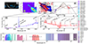 |
Fig. 1. Work overview. From left to right and top to bottom: Labeled panels show: a) S-PLUS footprint scan over the southern hemisphere, where each light blue square represents a single S-PLUS observation (FoV of 1.4 × 1.4 deg2). b) Zoom-in on the S-PLUS field where NGC 253 is located, called field −s20s09, where an inset provides a closer view into the nuclear regions of this galaxy. Within the latter inset, there is another inset zooming in toward NGC 253’s CMZ, which is shown in the next panel. c) Here, we indicate the Hα (MUSE) emission as red contours and shaded areas, showing the strong stellar outflow observed at optical wavelengths. Complementing the latter, in the same panel, we show mainly in blue and white the integrated intensity of the CN 1–0 line at ∼113.4 GHz taken from ALCHEMI observations at 1 |

2.1. S-PLUS
The Southern Photometric Local Universe Survey (S-PLUS; Mendes de Oliveira et al. 2019) will cover ∼9300 deg2 of the southern hemisphere (currently 80% complete), employing seven narrow-band and five broad-band filters, encompassing a wavelength range from 3533 Å (u filter) to 8941 Å (z filter). The survey uses a dedicated robotic telescope of 0.8 m called T80-South, at the Cerro Tololo Inter-American Observatory (CTIO) in Chile. The angular resolution is subject to weather conditions, with a typical seeing range of 0 8 to 2
 0 and an average of 1
 5.
5.
For this work, we used images in all 12 available filters from the S-PLUS fifth data release (available for internal collaboration), maintaining a consistent angular resolution of 1 5 (∼25.4 pc). For further details on the S-PLUS survey, we refer to Mendes de Oliveira et al. (2019) and Herpich et al. (2024).
2.2. VLT and HST
This study incorporates the dataset presented in Fernández-Ontiveros et al. (2009), including Adaptive Optics images from the Very Large Telescope/NaCo (VLT/NaCo) and diffraction-limited images from VLT/VISIR and the Hubble Space Telescope (HST). We refer to Fernández-Ontiveros et al. (2009) for further details.
The VLT/NaCo observations were conducted on December 2 and 4, 2005, utilizing the IR wavefront sensor (dichroic N90C10) for atmospheric correction. The observation included the following filters and integration times: J (600 s; 3% Strehl ratio1), Ks (500 s; 20% SR), L (4.375 s; 40% SR), and NB_4.05 (8.75 s, centered on Brα; 40% SR). The resulting images achieved different FWHM resolutions: 0 29 (J), 0
 24 (Ks), 0
 13 (L), and 0
 14 (NB_4.05). Images from VLT/VISIR, captured on December 1, 2004, and October 9, 2005, encompassed the N (PAH2_2, λ11.88 μm, δλ0.37 μm; 2826 s) and Q (Q2, λ18.72 μm, δλ0.88 μm; 6237 s) bands. The achieved FWHM resolutions were 0
 4 (N) and 0
 74 (Q). Furthermore, HST images were utilized within the central ∼300 pc region of NGC 253, employing the F555W (V band, FWHM = 0
 11), F656N (Hα, 0
 22), F675W (R band, 0
 20), F814W (I band, 0
 13), and F850LP (0
 13) filters.
2.3. Spitzer/IRAC
We retrieved Spitzer/IRAC mosaic images from the Spitzer Heritage Archive2. The mean FWHM of the point spread function (PSF) of the four IRAC bands at 3.6, 4.5, 5.8, and 8.0 μm are 1 66, 1
66, 1 72, 1
72, 1 88, and 1
 98, respectively (Fazio et al. 2004, their Table 3). Thanks to the large field of view (FoV) of Spitzer, which covers the entire emission from NGC 253, we were able to use data from these four IRAC filter images in all our GMCs.
2.4. ALMA
ALMA observations of NGC 253 were conducted during Cycles 5 and 6 as part of the ALCHEMI large program. The observations consisted of an unbiased complete spectral scan across the ALMA bands 3 to 7 (84–373 GHz, λ = 3.6–0.8 mm) across the whole CMZ region (inner 500 pc; Sakamoto et al. 2006) of the galaxy. The observations were carried out using both 12m and 7m antenna arrays aiming to retrieve extended emission, and the data were imaged to common angular and spectral resolutions of 1 6 and ∼8–9 km s−1, respectively. The flux density root-mean-square (RMS) noise ranges from 0.18 to 5.0 mJy beam−1 in the 8–9 km s−1 channels. In Fig. 2, we provide the integrated intensity maps of the continuum emission (in mJy) of the CMZ of NGC 253 at ALMA bands 3, 4, 6, and 7 (100, 144, 243, and 324 GHz, respectively).
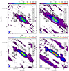 |
Fig. 2. Integrated intensity maps of NGC 253’s CMZ showing its ten GMCs at the central frequencies of ALMA bands 3, 4, 6, and 7 (i.e., at 100, 144, 243, and 324 GHz). Data from ALMA band 5 are not shown as its central frequency of 187 GHz is strongly affected by telluric absorption from a water line at ∼183 GHz, as can be inferred from Fig. 1. The ALCHEMI 1 |


The absolute flux density uncertainty was reported to be of order 10 to 15%. We assumed a conservative uncertainty of 15% for our extracted ALCHEMI fluxes. However, the relative flux uncertainty within the individual ALCHEMI observations is 2 − 3% after the alignment performed on the data enabled by the continuous frequency coverage. A full description of the dataset, calibration, and imaging is provided by Martín et al. (2021).
2.5. EVLA
We obtained archival data from the Expanded Karl G. Jansky Very Large Array (EVLA) in two different ways. The first approach was to directly search the VLA archive. In this way, we obtained the reduced NGC 253’s CMZ image in the X band at 3 cm (PI: N. Harada), which has been observed in A configuration mode, leading to a largest angular scale (LAS) of 5 3 according to the EVLA documentation3. We applied a cleaning to these data using tclean with a standard gridder and a hogbom deconvolver inside the Common Astronomy Software Applications (CASA) package4. In addition, we used a 1 cm (33 GHz; Ka band) continuum image presented in Kepley et al. (2011). These observations were done at DnC hybrid configuration, which leads to a LAS of 44″5. We used CASA imsmooth to convolve the X band EVLA continuum image to a common circular beam of 1
 6, matching that of ALCHEMI. In the same way, for the Ka band (26.5–40.0 GHz) image, we chose a slightly larger (1
 8) beam due to an original beam of 1
 76 × 1
 38. Since the images are in Jy/beam, we converted them into Janskys by dividing their flux by the beam area in pixels [pix/beam] available in the CASA Viewer (Statistics/BeamArea) panel. We note that the LAS, θLAS (see Table 2), is smaller than the aperture size for the Ka band observations. However, we did not see significant deviations of these observations with respect to the rest of the dataset. In fact, the model fits the observations quite well when they are available (GMCs 3–7). Any expected departure or uncertainty in flux is compensated for by the added uncertainties in our SED models, which is up to 30% for the case of GalaPy (Ronconi et al. 2024).
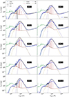 |
Fig. 3. SED models obtained with the GalaPy software for the ten GMCs studied in this work, each of them covering a diameter of 3″ (∼50 pc; see Sect. 3.1). Points correspond to the photometric measurements obtained from the sample (Sects. 2 and 4.1), while solid lines correspond to the unattenuated stellar emission (green), molecular cloud component (MC, purple), stellar emission considering extinction (extinct, red), and diffuse dust (DD, yellow). Best-fitting modeling results from CIGALE, devoid of an AGN component, are overlaid as solid blue lines (see also Fig. A.1 for a detailed view). Detailed information about the CIGALE modeling is given in Appendix A. |
2.6. VLA
We retrieved Karl G. Jansky Very Large Array (VLA) continuum maps processed with the AIPS VLA pipeline by Lorant Sjouwerman (NRAO) from the webpage6. Of those, VLA band L (VLA A conf.) is the only one where all the ten GMCs studied in this work are detectable. Details on the wavelengths, fluxes per GMC, array configurations, and FWHMs are summarized in Table 2. We find very good consistency between VLA and EVLA points, delivering similar fluxes within 1 or 2σ of the SED fitting. There is a noticeable missing flux in L-band for GMC 5 (see Fig. 3), which can be associated to the free-free absorption effect (e.g., Kellermann & Pauliny-Toth 1969) observed in compact IR-bright starbursts (Condon et al. 1991; Clemens et al. 2010; Dey et al. 2022).
Since we are considering flux densities, we decided not to convolve our VLA continuum maps, as we noticed that it can produce artifacts that may show up in GMC positions without clear emission, leading to false positives. Upon examining the summed fluxes within 3″ diameter apertures before and after convolution with CASA imsmooth, we observed differences of less than 10% (i.e., less than the instrumental uncertainties).
2.7. GMC positions
The selection of GMC positions to be analyzed in this study is driven by the ALMA data from the ALCHEMI project. Thus, we use the GMC positions determined by Harada et al. (2024), which incorporate both the continuum and molecular emission peaks – except for GMC 3, GMC 4, and GMC 10. For these three clouds, and given the similarity between the dataset used in Leroy et al. (2015) and the ALCHEMI data, A. K. Leroy (private communication) provided modified GMC coordinates tailored to the ALCHEMI data for the collaboration, which were retained for GMCs 3, 4, and 10. These three GMC positions were derived using CPROPS (Rosolowsky & Leroy 2006) considering intensity peaks of the CS J = 2 − 1 and H13CN J = 1 − 0 transitions.
Our region coordinates are close to those used by Leroy et al. (2015), whose reference coordinates are clarified in Behrens et al. (2022), specifically in their Appendix A. The differences between their coordinates and the ones we used in this study, listed in Table 1, are up to ∼1 3 in right ascension and ∼1
 4 in declination, corresponding to spatial offsets of up to 23 pc and 24 pc, respectively, at the assumed distance of NGC 253 of 3.5 Mpc. These variations fall within our photometric aperture radius of 25 pc.
The general reason for this selection is to avoid, as much as possible, overlapping between our apertures of 3″, while at the same time extracting most of the intensity in each aperture. We note that the variation in the GMC positions from different source extraction criteria is relatively marginal (∼0 2) compared to the apertures used in this paper. Alongside the course of this work, we will compare our GMC characteristics with those of the GMCs in previous ALCHEMI works with the same numbering, unless it is explicitly mentioned.
3. Analysis: SED and spectroscopic modeling
The main results from this study come from two methods used to explore in detail the spectroscopic and photometric information of the CMZ of NGC 253. We employed GalaPy for the photometry information, from NUV to centimeter (cm) wavelengths. To cross-validate the results obtained from GalaPy, we compared them with those from the broadly used Code Investigating GALaxy Emission (CIGALE). While CIGALE provides a refined treatment from the UV to the submillimeter (submm) regimes, it models the radio centimeter luminosities from star formation using the FIR/radio correlation coefficient (qIR) scaling relations. In contrast, GalaPy incorporates a full model based on the theoretical simple stellar population (SSP) approach from Bressan et al. (2002). It self-consistently incorporates nebular and synchrotron emission within the chosen star formation history (SFH) model. This makes GalaPy a powerful tool for gaining deeper insights into the link between radio emission andstellar populations. Given that our study relies on extensive radio data, we selected GalaPy as the primary tool for SED modeling, in particular, for testing the radio-SF correlation.
As we explain in Sect. 4.1, despite differences between the SED modeling codes (e.g., in our Fig. 3), we can confirm the nature of GMCs and many of their main physical properties; for example, the SFR and the stellar mass in the studied GMCs is higher toward the inner regions of the CMZ, independently of the code used. Nevertheless, we have found certain differences among the codes’ results, which reflects the range of possibilities one can obtain when depending on the used SFH model, mass-luminosity relation, and IMF, among other assumptions.
Additionally, to complement this study, we applied STARLIGHT for the spectral MUSE data plus photometric (S-PLUS) information in the NUV to NIR range. Below, we elaborate on our procedures. In Fig. 3 we provide our best-fit models to the extracted flux densities summarized in Table 2. This Figure primarily shows GalaPy results but also presents the CIGALE best-fit models (solid blue lines). CIGALE best-fitting results are further provided in detail (i.e., with all the considered components) in Fig. A.1.
3.1. GalaPy photometric SED fitting
We performed the SED fitting of our selected GMCs with GalaPy (Ronconi et al. 2024), an open-source application programming interface developed in Python/C++ across a range from X-ray to radio frequencies. GalaPy assumes a Chabrier initial mass function (IMF; Chabrier 2003) and a flat ΛCDM cosmology with approximate parameters: matter density around 0.3, baryonic density around 0.05, and a Hubble constant H0 = 100 h km s−1 Mpc−1, where h is roughly 0.7 (Planck Collaboration VI 2020). GalaPy is expected to include tools for optical spectroscopy and an AGN component on top of its SED fitting algorithm, although these modules were not available at the time this work was initiated. In the subsequent subsections, we detail the relevant configurations pertinent to the objectives of this study.
3.1.1. The in situ model
GalaPy allows the user to choose among a range of SFH models, both empirical and non-parametric. For our models, we used the default in situ SFH model, which has proven successful in predicting the emission from both late and early type galaxies in the local Universe as well as for young highly star-forming systems up to high redshift (Pantoni et al. 2019; Giulietti et al. 2023; Ronconi et al. 2024; Gentile et al. 2024). The physically motivated in situ model, developed by Lapi et al. (2018), adopts a SFR (ψ(t)) of:
 (1)
(1)
with x ≡ τ/sτ⋆, where τ is the galactic age, τ⋆ is the characteristic star-formation timescale, s ≈ 3 is related to the gas condensation, and γ is related to the gas dilution, recycling, and stellar feedback (see Lapi et al. 2020, for more details).
In the in situ model, the evolution of the gas and dust masses and of the gas and stellar metallicities can be followed analytically as a function of the galactic age, and self-consistently with respect to the evolution of the SFR. This means that an isolated system is assumed for each molecular cloud (MC), implying an interdependence among parameters. For example, a correspondence between metallicities and ages. This approach guarantees that the derived physical properties that directly result from the evolution of the stellar population (e.g., the components’ masses and metallicities), are consistently propagated to the other models contributing to the overall emission of the object.
3.1.2. Simple stellar populations
Among the available Simple Stellar Population (SSP) libraries in GalaPy, we have selected the “refined” version of parsec22.NTL (Bressan et al. 2012; Yan et al. 2019; Ronconi et al. 2024) as our preferred choice. This library ensures a dense wavelength grid with a minimum of 128 values per order of magnitude within its 2189-point grid. It incorporates emission from dusty Asymptotic Giant Branch (AGB) stars and accounts for nebular emission and free-free continuum in addition to the stellar continuum and non-thermal synchrotron radiation from core-collapse supernovae.
For the purposes of our study, the parsec22.NTL SSP library was modified to correctly process the photometric points obtained from the narrow bands of the VLT/VISIR instrument (see Sect. 2.2). This adjustment will be available in the next release of GalaPy.
3.1.3. Dust model
GalaPy implements an age-dependent two component dust model which is constructed in order not to assume an attenuation curve but to derive it instead from structural parameters (e.g. density and extension) which can be obtained by tuning the model to best represent an observed dataset.
The two different components comprise the contribution of (1) a hot molecular cloud phase (normally referred in the literature as a “birth-molecular cloud;” see, e.g., Charlot & Fall 2000) of new stellar populations and (2) a diffuse and extended dusty medium which further attenuates the stellar emission. Both components also contribute to the IR emission which is then the combination of two separate modified graybodies.
GalaPy common inputs.
GalaPy varying inputs.
Among the several possible free parameters on which this dust model depends, we chose to fix some known values and ranges, in order to both ensure physically plausible results and speed up the computing process. This consists in setting a range of reliable physical terms, such as the total number of molecular clouds to NMC = 1, as in this work we are assuming isolated GMCs, and their dusty and molecular radii, which were set to be within a 10–100 pc range, although they will likely be closer to the lower limit considering the 30 pc diameter inferred from their sub-mm emission (Leroy et al. 2015). A list of all common parameter ranges and individual values used to model the SEDs in the ten GMCs is provided in Table 3. There, the redshift was taken from the SIMBAD Astronomical Database (Wenger et al. 2000). These ranges are fixed for all GMCs. On the other hand, the parameters that were fine-tuned for specific GMCs along with their corresponding adjusted ranges are presented in Table 4. The parameters listed in this second table vary across different GMCs, with their respective ranges for each GMC. For example, the range of the molecular cloud radius, RCM (pc), was fine-tuned and is set between 0.0 and 1.7 for GMCs 2 and 8, while for the other GMCs, this radius remains between 0.0 and 2.0 (in log10 scale).
We use different initial conditions for unknown parameter ranges such as the GMC ages (age), the time of maximum star-formation (sfh.tau_star), the time that stars need to escape from its parental molecular cloud (ism.tau_esc), the maximum SFR (sfh.psi_max), and the average radius of the molecular cloud (ism.R_MC). We mainly modified the R_MC, ism.R_MC, and sfh.psi_max in cases where the results were bimodal, in order to achieve a single result in the parameter space distribution. For example, the R_MC was fixed to not exceed 50 pc in GMCs 2 and 8, motivated by Table 3 in Leroy et al. (2015), where their molecular radii are expected to be around 52 and 44 pc, respectively. Interestingly, these two GMCs are the largest in the sample, according to the mentioned study.
We recommend consulting Table B.3 in Ronconi et al. (2024) for a complete description of all GalaPy parameters. This table is also described on the project’s ReadtheDocs web page7. The information there goes beyond what is covered in the present work, which is limited to the in situ model.
3.2. CIGALE photometric SED fitting
In addition to the main results obtained from GalaPy, for comparison we also provide simultaneous UV-to-radio SED modeling with the CIGALE 2022.1 version (Yang et al. 2022). This software operates on the principle of energy balance, where energy attenuation in the UV-to-optical range is re-emitted in the infrared in a self-consistent manner. Its modular and parallelized design, along with its user-friendly interface, has made it a popular choice in the literature for estimating the astrophysical characteristics of various targets. Below, we provide a brief overview of the models employed to simulate the galaxy emission.
To construct the SEDs with CIGALE, we utilized the full photometric coverage available for our GMCs. The modeling was based on the widely-used Bruzual & Charlot (2003) SSPs, adopting the IMF of Chabrier (2003) and assuming a solar-like metallicity. The stellar populations evolved using a delayed SFH, a model in which the SFR initially rises, peaks after a delay, and then declines exponentially, with an additional burst component (Ciesla et al. 2015). This SFH approach is more realistic compared to the simple delayed model and has been demonstrated to minimize biases in the estimation of SFR and stellar mass (Schreiber et al. 2018). Additionally, the inclusion of the burst is consistent with the ALMA detections (Hamed et al. 2021, 2023). For the SFH parameters, we maintained flexibility in the age and the e-folding time of the main stellar population to avoid introducing artificial biases in the efficiency of the initial burst.
Dust attenuation was modeled following the Calzetti et al. (2000) attenuation law, allowing for the color excess of the young stellar population to vary as a free parameter. Dust emission was a critical component of our SED modeling, given the extensive IR coverage, particularly from ALMA. We used the models provided by Draine et al. (2014). To ensure a good fit, we explored the parameter space for PAH fractions and the radiation field, Umin, aiming to minimize χ2 while keeping the models physically realistic. Considering the rich radio data available for the GMCs, we extended our UV-IR modeling to the radio regime taking into account the power-law nature of the synchrotron spectrum and the ratio of the FIR/radio (qIR) correlation in the CIGALE fitting.
CIGALE minimizes χ2 by measuring the difference between observed data and the model predictions, weighted by the uncertainties in the observations. The goal of minimization is to find the best-fitting model parameters that reduce this difference (Boquien et al. 2019). Additional details, including the addition of AGN-related parameters, are provided in Appendix A.
3.3. Stellar population fitting with STARLIGHT
GalaPy and CIGALE are used in the full SED fits (all wavelengths from UV to radio), while STARLIGHT will be used for the optical data only to fit stellar population models. STARLIGHT has been successfully applied to fit the stellar component of a diverse range of galaxy types, such as low-luminosity AGN, Seyfert nuclei, and normal galaxies (Cid Fernandes et al. 2005, 2013; Krabbe et al. 2017).
While it has traditionally been used for optical spectra, we applied the latest version of the code, described by Werle et al. (2019), to fit simultaneously the combined MUSE and S-PLUS data, thereby covering the 3500–10 000 Å range. The combination of these datasets provides a comprehensive view of the galaxy’s stellar populations, spanning a wide range of wavelengths. In particular, the S-PLUS bands densely cover the highly informative region around the 4000 Å break which falls outside the range of MUSE spectra that start at 4600 Å.
GalaPy results for star-formation-related properties.
STARLIGHT uses a chi-squared minimization technique to find the best-fit non-parametric combination of stellar populations of different ages and metallicities from a pre-defined library. This analysis allows us to estimate a number of properties, such as mean age, metallicity, and extinction, as well as the velocity dispersion of the stellar component. The base is built from SSP models from the Charlot & Bruzual 2019 library models (Martínez-Paredes et al. 2023) using PARSEC (PAdova T Rieste Stellar Evolution Code) evolutionary tracks (Bressan et al. 2012; Chen et al. 2015) and a Chabrier IMF. A base of composite stellar population is built from the SSP models assuming constant SFRs in 16 logarithmically spaced age bins with 5 different metallicities. Extinction is modeled with two components: one applied to all populations (AV) and an extra one applied exclusively to ≤10 Myr old stars (δAV). The list of parameters to fit includes the flux (or mass) fractions of the different populations, global and selective extinction, the velocity shift, and velocity dispersion.
We adjusted the weight scheme for the code used to extract residuals for Hα, [N II], [O III], and Hβ by augmenting them around those lines. This modification allows for a detailed examination on the contribution of stellar absorption features to these emission lines, compared to a general fit to the MUSE+S-PLUS spectra/photometry. These lines will subsequently serve as input for diagnostic diagrams and to estimate the extinction affecting the emission line regions.
4. Results
In the following, we supplement our SED analysis with existing results from the literature, including those obtained by the ALCHEMI collaboration. Since the GMC selection was based on ALMA observations, our primary sources of information are the ALCHEMI results (Martín et al. 2021). After detailing the characteristics of the ten GMCs by dividing them in two main groups, we will compare our panchromatic results – derived from SED fitting – on SFRs and SFHs with those obtained from pure-optical and pure-sub-mm/cm observations, that is, from monochromatic tracers such as the Hα and H40α emission lines and different infrared and radio continuum regimes or bands. This approach will help us understand the key limitations to consider when working with mono-wavelength datasets. For a more detailed description of our results in light of previous literature information and for each of the ten GMCs, we refer to our Appendix B.
4.1. SED fitting
The wealth of archival data described in Sect. 2 does not always cover the ten GMCs. Only the S-PLUS, Spitzer/IRAC, ALCHEMI, VLA L (1.5 GHz), and Ku (15 GHz) bands fully cover the NGC 253’s CMZ (see Table 2). EVLA band X does not detect emission outside GMCs 3 to 6, similar to the case in VLA K (23.6 GHz) band observation, which also detects emission only in GMCs 3 to 6. Also, the VLA C (4.9 GHz) band does not detect emission in GMCs 1 and 2, and our aperture of 3″ is not fully covered by emission in GMCs 8–10, hence we discarded the latter contribution. From the above, we can say that the best-studied GMCs are GMCs 3 to 6, corresponding to the core of NGC 253 and encapsulating most of the star formation activity across the central starburst region (Bendo et al. 2015). It is worth saying that, in addition to the possible lack of continuum emission, the not imaged/detected GMCs may fall below the detection limit of our ALMA band 3 observations and the different centimeter bands mentioned above. The detection limit at 3σ of EVLA band X, and VLA bands K and C are 2.4 × 10⁻², 5.4 × 10⁻³, and 6.6 × 10⁻⁴ Jy, respectively.
In general, the GMC’s SED shapes (shown in Fig. 3) are similar to what is found in local and high-redshift starbursts (e.g., Swinbank et al. 2010). These SEDs exhibit significant absorption in the NUV and optical wavelength regimes (∼3 × 10³–104 Å), caused by an exceptionally large amount of dust. This leads to a substantial difference between the predicted and observed emissions (i.e., stellar emission with and without extinction), illustrated by the red and green lines in Fig. 3. At the mentioned wavelengths, the flux difference can reach up to four orders of magnitude (e.g., from ∼103 mJy down to ∼10−1 mJy in GMCs 4–6 at 104 Å). The total extinction (Av) derived from the stellar component exceeds 5.0 magnitudes in GMCs 3-6, based on analyses from GalaPy, CIGALE, and the Balmer lines (Hα and Hβ; see Sect. 4.2.2).
Tables 5 and 6 respectively contain GalaPy and CIGALE results related to star-formation processes, such as the SFR, the stellar mass (M★), the characteristic timescale (τ★), or the stellar age (Age). In addition, results on the gas and dust characteristics, the attenuation, the radiation field (Umin), the time for stars to escape from their parental MC (ism.tau_esc), and uncertainties of the model, to mention a few, are given in Tables B.1 and A.3 for GalaPy and CIGALE, respectively.
CIGALE results for star-formation-related properties.
We summarize below the main characteristics of the molecular clouds studied here by dividing them into two groups: the central GMCs, numbered from 3 to 6, and the external ones, GMCs 1, 2, and 7–10. We find strong differences among them in terms of stellar and dust masses, and SFRs. Appendix B provides detailed information of individual GMCs.
4.1.1. GMC characteristics
The CMZ of NGC 253 can be divided into two primary groups based on the physical and chemical properties found in their GMCs: internal and external GMCs. The internal GMCs, corresponding to GMCs 3, 4, 5, and 6, are located in the very nuclear region of the CMZ, about 120 pc extension (see, e.g., the scale bar in Fig. 11), and are characterized by a large occurrence of molecular tracers indicating high densities (ngas > 107 cm−3), elevated temperatures (Tkin > 100 K), and strong and fast shocks (vshock ≳ 15–20 km s−1) likely triggered by a tremendous star formation activity (Meier et al. 2015; Bouvier et al. 2024; Bao et al. 2024).
Conversely, the external GMCs encompass GMCs 1, 2, 7, 8, 9, and 10, located near (GMC 7) or fully immersed in the periphery of the internal bar. We note that, unlike some ALCHEMI studies (e.g., Huang et al. 2023) but in line with others (e.g., Harada et al. 2024), based on the findings of the current study (i.e., SFR, dust (Mdust), and stellar (M★) mass), GMC 7 is better defined as an external region (see the text below and also Fig. 4). Due to their locations, these external GMCs may experience the effect of orbital intersections such as inner Lindblad resonances (Iodice et al. 2014), bar/spiral arm interactions –also known as x1/x2 interactions (e.g., Kim et al. 2012)–, and cloud-cloud collisions (Ellingsen et al. 2017, see their Sect. 4.3) take place (see, e.g., ellipses in Fig. 2). These GMCs are dominated by a lower-density molecular gas, as compared to the internal GMCs, and exhibit signatures of slow shocks (up to ∼15 km s−1) rather than intense stellar feedback. This division reflects significant dynamical and chemical variations across the CMZ, previously noted by ALCHEMI studies (e.g., Tanaka et al. 2024; Behrens et al. 2024; Harada et al. 2024).
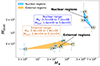 |
Fig. 4. Stellar and dust masses of the analyzed GMCs derived by GalaPy (see Subsect. 4.1.1). Their different ranges are indicated in the central labels. |
The study by Harada et al. (2024) utilized ALMA observations to conduct a detailed survey of molecular lines, applying principal component analysis (PCA) to distinguish patterns of chemical excitation and physical conditions across the CMZ. Their results indicate that the internal GMCs (GMCs 3–6) exhibit strong emissions from dense gas tracers such as HCN and HC3N, along with radio recombination lines (RRLs), which are associated with active star formation and high-excitation regions (e.g., Bendo et al. 2015). In contrast, the external GMCs (GMCs 1, 2, and 7 to 9 in the work of Harada et al. (2024), which did not account for GMC 10) are characterized by tracers of slow shocks, such as CH3OH and an increment of HNCO over SiO (Meier et al. 2015; Humire et al. 2022), reflecting less energetic dynamical processes. The PCA revealed that molecular emission correlates strongly with dynamical features, with high-excitation species dominating the central regions, while shock tracers are more prevalent in the outskirts.
In the current analysis, the differentiation between internal and external GMCs is further supported by variations in SFR, stellar mass, and dust mass. The internal GMCs exhibit SFRs above 0.087 M⊙ yr−1, as found by GalaPy, which provides an instantaneous SFR listed in the second column of Table 5. They also have greater stellar masses (third column; Table 5) and dust masses (Mdust; Table B.1) compared to the external GMCs. This is consistent with the high-density, high-excitation environments described by Harada et al. (2024).
For the sake of clarity, we provide a plot showing the dust mass, Mdust versus stellar mass Mstar in Fig. 4, from GalaPy. In the latter figure, we label the ranges for these quantities for nuclear and external regions or GMCs. The internal or nuclear GMCs (GMCs 3–6) display stellar masses in the 3.7 –7.1
–7.1 range, and dust masses in the 1.6
 –5.8
–5.8 range, in strong contrast to the external GMCs, where the stellar and dust masses range between 0.034
 –1.4
–1.4 and 2.6
 –4.8
–4.8 104 M⊙, respectively.
The above indicates that the dust mass is the clearest distinction between the two primary groups, while the stellar mass, although enhanced in the internal GMCs, is only a factor of two larger in GMC 6 (internal) with respect to GMC 7 (external).
The external GMCs are also characterized by a lower SFR than the inner ones, with values in the 0.005–0.022 M⊙ yr−1 range. These findings align with the chemical and dynamical distinctions previously observed in multiple ALCHEMI studies (e.g., Tanaka et al. 2024; Behrens et al. 2024; Harada et al. 2024), reinforcing the conclusion that the physical properties of the CMZ are tightly coupled with its molecular and dynamical characteristics.
4.2. Optical spectral fitting
We fit archival MUSE data (ID:0102.B-0078(A), PI: Laura Zschaechner) in the 4600–9350 Å range with S-PLUS photometric data using STARLIGHT (Cid Fernandes et al. 2005) in its latest version which is capable to fit spectra and photometry simultaneously (López Fernández et al. 2016; Werle et al. 2019).
To correct for the mismatch between spectroscopic and photometric fluxes, we scale MUSE spectra to match the iSDSS band flux of S-PLUS. The S-PLUS bands used for the fits are uJAVA, J0395, J0410 and J0430, iSDSS. The filter F0378 was not used to avoid contamination by [O II] 3727 emission. Of these, the blue ones are the most important, because they extend the MUSE coverage to the age sensitive 4000 Å region.
The STARLIGHT fits to the MUSE spectra and the fitted S-PLUS photometric points for the ten GMCs are shown by the blue lines and the cyan points, respectively, in Fig. 5. Some important stellar absorption features are labeled in the top panels and indicated by vertical dashed green lines for all the GMCs. The outputs of the fitting are summarized in Table 7.
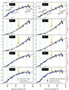 |
Fig. 5. STARLIGHT fits (shown by blue lines) are applied to the MUSE spectra (represented in black, with yellow lines indicating masked data) along with S-PLUS photometry fits (depicted with black and red circles, depending on whether they were used in the fit, with red points marking the masked data, and cyan points for the S-PLUS photometric data fitted by STARLIGHT). Vertical dashed lines indicate the position of the stellar features labeled in the top panels. |
Best-fitting results derived for each studied GMC by STARLIGHT.
As is commonly known (see, e.g., Conroy 2013), low-mass stars dominate both the total mass and the number of stars in a galaxy, but they contribute only a small fraction to the overall light output, or bolometric luminosity, since young stars outshine older stars. This can be seen in the star formation histories per GMC, which are plotted in Fig. 6. Independent of the molecular cloud, the light fraction is always shifted toward young stars, while the mass fraction is concentrated in old stars. For example, in GMC 5, nearly 100% of the stellar mass was already formed 10 Gyr ago while ∼50% of the light comes from stars younger than 30 Myr.
Also in Fig. 6, for GMC 5, we have over-plotted (in magenta) the normalized skewed Gaussian derived from the age-metallicity relation (AMR; see Appendix C). This same distribution was adapted to be cumulative (cAMR) and plotted (in yellow). GMCs 3 to 6 also show the estimated ages from super star clusters derived by Butterworth et al. (2024) in vertical dashed blue lines.
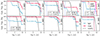 |
Fig. 6. STARLIGHT and GalaPy star-formation histories for the GMCs studied in this work. STARLIGHT discriminates between light and mass contributions to the total emission, contribution mainly coming from recent (blue) and old (red) stellar populations, respectively. GalaPy (black) generally provides ages between STARLIGHT’s light- and mass-weighted ages. For GMC 5, we have over-plotted the cumulative (in yellow) and normalized (in magenta) skewed Gaussian derived from the age-metallicity relation (see Appendix C). GMCs 3 to 6 also show the estimated ages from super star clusters derived by Butterworth et al. (2024) in vertical dashed blue lines surrounded by 1σ uncertainties as shaded areas; the remaining cumulative fraction (Cum. Frac.) to reach 100% of the emission at those ages, that is to say, the percentage of stellar formation that these radio observations account for, are denoted as r.l.f. and r.m.f. for remaining light and mass fractions, respectively. |
In most cases (GMCs 1–9), GalaPy yields stellar age estimates that are consistent with those from STARLIGHT, falling between the young and old stellar populations that best reproduce the optical stellar contribution modeled by STARLIGHT. This is more clearly seen in Fig. D.2, where we plot, for all ten GMCs studied in this work, the average old and young stellar population ages from STARLIGHT, and the global stellar ages from GalaPy. Both codes agree in that GMC 4 is the youngest in the sample, with younger stellar populations in GMCs 3 to 7 and older ones located in GMCs 1, 2, and 8 to 10. In addition, in the same plot we added results from CIGALE, whose output delivers youngest ages in general with the youngest stellar burst in GMC 5, very close to the youngest burst in GMC 4 derived by GalaPy.
4.2.1. Emission line diagnostic diagrams
The fluxes of emission lines from the MUSE spectra were measured in the pure nebular spectra, which were obtained by subtracting the stellar population continuum from the observed spectra. The contribution of the stellar population was determined using the stellar population synthesis code STARLIGHT (Cid Fernandes et al. 2005).
We show our results in Fig. 7, where we extract the emission lines in our common 3″ diameter aperture using archival MUSE observations (PI: Laura Zschaechner). Fig. 7 displays two diagnostic diagrams to analyze the dominant ionization mechanism of the emitting gas in the galaxy:
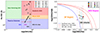 |
Fig. 7. WHAN (left) and BPT (right) diagnostic diagrams (see Sect. 4.2.1) for the ten GMC studied using emission line ratios of the optical spectra from MUSE. We prefer the term “starburst+shocks” (SB+Shocks) over the commonly used “composite” given the findings highlighted in Sect. 4.2.1. |
-
The [O III] λ5007/Hβ versus [N II] λ6584/Hα diagnostic diagram proposed by Baldwin et al. (1981), commonly known as the BPT diagram. This diagram includes the theoretical separation between H II-like and AGN-like objects proposed by Kewley et al. (2001a) [K01], and the empirical star-forming limit proposed by Kauffmann et al. (2003) [K03]. The region between the theoretical and empirical limits is commonly referred to as the “composite region,” although there are claims against this designation (see below).
-
The WHAN diagram, namely, log(EW Hα) versus log([N II]λ6584) (Cid Fernandes et al. 2010), which is used to differentiate the nature of the ionization sources, classifying objects as star-forming, strong AGNs, weak AGNs, or retired galaxies. The line at log(EW Hα) = 6 Å represents the limit between weak and strong AGN emission. We note that in this diagram, the chosen log10([N II]λ6584/Hα; x-axis) limit to disentangle between SF and AGN gaseous ionization origin is normally taken from Stasińska et al. (2006) [S06] in the literature, although for NGC 253’s CMZ we can rely on K03 as there are no GMCs between S06 and K03 limits.
Although molecular gas and star-forming regions are known to spatially decorrelate at sub-100 pc scales (e.g., Kruijssen & Longmore 2014; Chevance et al. 2020), in the CMZ of NGC 253, we do observe gas and dust in regions where star formation is taking place, especially in the inner regions (e.g., Bendo et al. 2015; Ando et al. 2017; Rico-Villas et al. 2020) (see also the super star clusters in Fig. 2). Nevertheless, our GMCs do not occupy the regions in these diagnostic diagrams that are typically associated with star-forming regions. Instead, they are located in what is often referred to as the “composite” zone, lying between star-forming and AGN-dominated areas. According to some studies, this behavior can occur in starbursts where stellar shocks are strong (e.g., Kewley et al. 2001b), and we consider this as the most likely scenario for the CMZ of NGC 253, which is also consistent with recent ALCHEMI studies on shocks (e.g., Bao et al. 2024; Bouvier et al. 2024). However, we cannot completely discard a decorrelation between star-forming regions and molecular gas in our line of sight given the large inclination (70°–79°; e.g., Pence 1980) of NGC 253.
However, given the lack of evidence for an actual AGN in NGC 253, and the fact that these line-ratios are observed well away from the nucleus, our GMCs are most likely not starburst+AGN composites. Instead, we prefer to describe them as “starburst+shocks” composites, where the observed line ratios are a mixture of star-formation and shocks from stellar winds and supernovae. Shocks are indeed known to be present in NGC 253 (Meier et al. 2015; Holdship et al. 2022; Humire et al. 2022; Behrens et al. 2022; Harada et al. 2022; Huang et al. 2023; Behrens et al. 2024; Bouvier et al. 2024; Bao et al. 2024), whereas there is extensive literature arguing against the presence of an AGN (e.g., Fernández-Ontiveros et al. 2009; Brunthaler et al. 2009; Müller-Sánchez et al. 2010).
From the SED perspective, a clear argument against the existence of an AGN is provided in Appendix A, where the AGN fraction, fAGN in Table A.4, is negligible (< 7.5%) and also does not peak at the centrally located GMC 5 as one might expect in the presence of an AGN. Although this behavior could potentially suggest the presence of a low-luminosity AGN (LLAGN), it is more plausibly interpreted as an artifact of CIGALE’s attempt to accurately fit the AGN-free SED. Further arguments specifically against the presence of an LLAGN can be found, for instance, in Mangum et al. (2019, their Sect. 7.1).
4.2.2. Attenuation estimations
The attenuation from dust in H II regions can be estimated using the Balmer lines Hα and Hβ by contrasting their observed ratios with their expected ratios without attenuation. The intrinsic Hα/Hβ flux ratio is 2.86 under typical conditions of electron density (ne ∼ 100 cm−3) and temperature (Te ∼ 10 000 K), although variations in these conditions can change the ratio by up to 4% (Osterbrock & Ferland 2006). The so called Balmer extinction is given by
 (2)
(2)
where AHβ/AV = 1.14 and AHα/AV = 0.82 for a Calzetti et al. (2000) reddening law. In the following, we will apply this method to the GMCs studied in this work by measuring (FHα/FHβ)obs for each region and estimating their respective attenuations.
For comparison, we also considered the attenuation model proposed by Charlot & Fall (2000), a widely used approach for estimating dust extinction in stellar populations. This method distinguishes between the contributions of young and old stellar populations, assigning different power-law attenuation slopes to each. The attenuation for young populations, attributed to birth clouds, is represented by αBCs, while that for older populations, associated with the ISM, is denoted as αISM, as described in Eq. (4). According to this framework, stars are initially formed within interstellar birth clouds (BCs) and migrate to the ISM after approximately 107 years. The transition between these two attenuation regimes occurs at a wavelength of 5500 Å. In CIGALE, this model can be adopted using the dustatt_2powerlaws module. The functional form of the law is commonly expressed in the literature as:
 (3)
(3)
where Aλ is the wavelength-dependent attenuation expressed as  , with λV = 5500 @@@, and AV represents the attenuation in the V band. In practice, this translates to the following expression:
![Mathematical equation: $$ \begin{aligned} A(\lambda ) = A_\mathrm{V} \left[ \left( \frac{\lambda }{\lambda _0} \right)^{\alpha _{\rm {BCs}}} (\lambda < 5500 \, {\AA }) + \left( \frac{\lambda }{\lambda _0} \right)^{\alpha _{\rm {ISM}}} (\lambda \ge 5500 \, {\AA }) \right], \end{aligned} $$](/articles/aa/full_html/2025/07/aa53897-25/aa53897-25-eq109.gif) (4)
(4)
where AV is the overall attenuation at 5500 Å that we assume to be unity for simplicity. The exponents αBCs and αISM describe the slopes for the birth clouds and the ISM, respectively. In the implementation, the values for αBCs range from –0.69 to −0.9, while αISM ranges from –0.75 to –0.3. We find these values starting from those commonly used in Charlot & Fall (2000) and also being influenced by other works that assume a –0.7 (an original assumption from C&F 2000) value for both stellar populations. Then, looking at our GalaPy-derived curves from the SED, we set values that better reproduce the observations.
We compute the attenuation curves over a wide wavelength range, from the NUV to the NIR, using these parameter ranges. The curves are normalized at 5500 Å to allow for a consistent comparison. As shown in Fig. 8, the model’s attenuation curves are sensitive to the chosen values of RV for the Calzetti et al. (2000) attenuation law, which assumes a single attenuation slope for all stellar populations, and the values of αBCs and αISM in the case of the Charlot & Fall (2000) models. The better agreement of our model-inferred attenuation laws with the Charlot & Fall (2000) prescription compared to Calzetti et al. (2000) stems from fundamental differences in their treatment of the star-dust geometry, which are particularly critical in the dense, young stellar environments of NGC 253’s GMCs. While Calzetti et al. (2000) provided a robust empirical description for homogeneous starburst systems by assuming a single attenuation component with a gray slope (RV ∼ 4.05) and suppressed 2175 Å UV bump (Conroy 2013; Salim & Narayanan 2020), it fails to capture the spatially segregated attenuation effects expected in galaxies with distinct birth clouds and diffuse ISM components. Our results align with theoretical studies demonstrating that the two-component Charlot & Fall (2000) models – which separate the attenuation between optically thick birth clouds and a diffuse ISM with shallower attenuation – better reproduces the observed SEDs of systems with ongoing star formation in dense environments. This is consistent with NGC 253’s molecular clouds, where young stars remain embedded in their natal dusty clouds, creating a non-uniform attenuation geometry that the Calzetti law’s simplified single-screen approximation cannot adequately model. The widespread adoption of the Calzetti law in literature reflects its utility for global galaxy-scale attenuation in starburst-dominated systems, but our findings emphasize that its limitations become pronounced in resolved studies of individual star-forming regions.
Table 8 lists the measured Balmer decrement, the corresponding  , as well as the AV values obtained with CIGALE and STARLIGHT. As expected from the extremely red shape of the optical spectra (see Fig. 5), we obtain large values of
  : from 1 to 6 mag. The largest values are found for GMCs 3, 4, 5, and 6, which are closer to the galactic bar and in dense star-forming areas. We note, however, the very substantial uncertainties in (FHα/FHβ)obs (ranging from 10 to nearly 90%). These happen because of the weak Hβ emission, which is barely visible in most cases in Fig. 5.
GMC attenuations.
Table 8 further lists the STARLIGHT results for the extinction. In the case of STARLIGHT the table gives  , which we define as the average of the extinctions affecting all populations (AV) and that affecting only those younger than 10 Myr (AV + δAV), weighting them by the fluxes of the respective components as derived from the fits. Again, the extinction values are large (1.8–5.7 mag), as expected from the redness of the optical continuum. The derived values are close to, but in general somewhat smaller than those derived from the Balmer decrement. CIGALE values of AV are, in median, 16% lower than those from the Balmer decrement,
  . On the other hand, STARLIGHT-based values also differ from those of
  by a median value of 27%.
The only GMC where  exceeds
  is GMC 1. This discrepancy may suggest additional sources of attenuation, potentially linked to warm or dense dust. One possible explanation is the influence of strong shocks, which could sputter dust grains and enhance local dust densities. Supporting evidence for the presence of shocks in GMC 1 comes from its elevated SiO J = 5–4/HNCO (100, 10–90, 9) transition ratios observed at about 220 GHz (ALMA band 6). This region shows the highest ratio values, averaging around 1.3, as noted in the right panel of Fig. 11 in Humire et al. (2022). In contrast, the mean ratio in other regions is 0.5, excluding GMC 10, where this ratio cannot be measured. The above values have been derived using an aperture of 3
 0 and the coordinates from this work, listed in Table 1. These elevated ratios are well-known tracers of strongly shocked gas, indicating a prevalence of strong (traced by SiO) over weak/mild shocks (traced by HNCO). Additionally, GMC 1 hosts methanol masers with the strongest deviations from LTE expectations among the ten GMCs, as illustrated in the left panel of Fig. 13 in Humire et al. (2022). While these observations strongly point to the presence of shocks, they are not direct indicators of warm or dense dust. However, shocks may indirectly affect the dust environment by altering its spatial distribution or properties. Future studies are needed to assess whether gas and dust are tightly coupled in this region and to determine the extent to which shocks influence the observed attenuation.
We compared the stellar continuum attenuation in the V-band, AV, with the corresponding stellar color excess, E(B − V)s (represented by the attenuation.E_BVs parameter), both derived from the CIGALE spectral energy distribution fitting results (Tables 8 and A.2). We find that the ratio AV/E(B − V)s ranges from ∼4.0 to 6.3 across our sample. Notably, this ratio systematically differs from the value RV = 3.1 that was set as an input parameter in our CIGALE configuration.
This apparent discrepancy arises from the specific implementation within the dustatt_modified_starburst module used in our analysis. This module employs distinct attenuation laws for the stellar continuum and the nebular emission lines. The input parameter RV = 3.1, characteristic of the diffuse interstellar medium in the Milky Way (e.g., Cardelli et al. 1989), governs the shape of the Cardelli et al. extinction curve applied specifically to the nebular emission lines (as we selected Ext_law_emission_lines = 1). However, the attenuation affecting the stellar continuum (from which AV and E(B − V)s are primarily determined) is modeled using the empirical starburst attenuation law from Calzetti et al. (2000), which can be further modified by a power-law slope (δ) and a UV bump. The baseline Calzetti law itself possesses an effective ratio AV/E(B − V)≈4.05, inherently different from the Milky Way value. The flexibility introduced by the allowed modifications (δ and the UV bump) within the module accounts for the observed range of AV/E(B − V)s extending above this baseline value, consistent with the methodology described in Boquien et al. (2019, Sect. 3.4.2). Therefore, the AV and E(B − V)s values derived for the stellar component are not expected to follow the relation AV = 3.1 ⋅ E(B − V)s, but rather reflect the properties of the modified Calzetti law applied to the integrated starlight.
GalaPy derived attenuation curves are shown in Fig. 8, where curves indicate the attenuation in the visible band and legends show its value at 5500 Å, on a linear scale, to be compared with STARLIGHT outputs (Table 7). The results from this code are normalize at that wavelength value. RV values following Calzetti et al. (2000) are also included for comparison. These values describe the relationship between the total amount of dust extinction and the amount of reddening it causes in the context of the Milky Way’s dust extinction curve and corresponds to the ratio between the total extinction AV and the color excess E(B − V). Considering the ten GMCs studied, most RV values range between 6 and 9, far beyond the Galactic value of 3.1. Surprisingly, the extreme values are found in clouds located at the boundaries of the CMZ, with the highest RV values in GMCs 2 and 9. These clouds are closer to the modeled curves (dashed lines in the left panel of Fig. 8) corresponding to RV ∼ 8–9. In contrast, the lowest RV value is found in GMC 1, which is best matched by a modeled curve with RV ∼ 4.
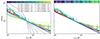 |
Fig. 8. Attenuation curves normalized at A(λ)/AV = 1 when λ = 5500 Å over wavelength in the rest frame, as derived by GalaPy SED fittings. The A(λ) value at 5500 Å is labeled in the legend of the left panel in linear scale and per GMC. This legend also indicates the color corresponding to each GMC in the solid lines. Curves based on RV values according to the methodology of Calzetti et al. (2000) are included for comparison (as dotted curves) in the left panel, following the colorbar. On the other hand, the dotted curves on the right panel show the attenuation curves from the models of Charlot & Fall (2000), which differentiate between young and old stellar populations, providing different exponential factors to the attenuation coming from birth clouds (BCs) and the ISM (ISM), related to these populations (see Sect. 4.2.2), which are labeled in the colorbar. |
As a final remark, when comparing the different attenuation estimates, it is important to recognize that the gas attenuation (from the Balmer decrement) and stellar attenuation (from GalaPy, CIGALE, and STARLIGHT in our case) have distinct origins. Recent studies suggest that these two types of attenuation should become increasingly similar as the observed region ages (Li & Li 2024).
However, we do not see a clear trend for attenuation differences between the ones derived from the Balmer decrement and those obtained from CIGALE, namely  , taken from Table 8, versus derived stellar ages from either GalaPy or CIGALE (last columns of Tables 5 and 6, respectively), we do see a trend when comparing attenuation differences between Balmer lines and the gas attenuation derived from the stellar continuum by STARLIGHT, namely
  , versus stellar ages derived by CIGALE. For an easy visualization of that finding, in Fig. 9 we present such a relation.
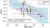 |
Fig. 9. Relation between absolute attenuation differences, |Δ AV|, obtained from the Balmer decrement, |

4.2.3. Linear regression
The procedure for all linear regressions in this work, including Fig. 9, followed two main steps. First, we used the linregress function from the scipy Python library to obtain initial priors. For power-law relationships, we performed the regression in log-space when required (using log10 values as inputs), with results either maintained in logarithmic form (log y = mlog x + c) or converted back to linear space depending on the analysis.
The second step applied Bayesian inference through a Markov chain Monte Carlo (MCMC) sampling using the emcee Python package (Foreman-Mackey et al. 2013). Unlike linregress, MCMC incorporates uncertainties in both axes (x and y), which were rigorously included in our modeling. We ran 1000 iterations per fit with 50 walkers, discarding the first 100 as burn-in to ensure convergence. The resulting posterior distributions provided robust estimates of the slope and intercept, with their 1σ uncertainties represented as shaded regions in all plots.
4.3. Star formation rates
4.3.1. Kennicutt (1998): Hα–SFR calibration
There are many ways to obtain the SFR from monochromatic emission. One of the most commonly used is the relation found by Kennicutt (1998) regarding Hα, which we will hereafter refer to as the “Kennicutt relation” as follows:
![Mathematical equation: $$ \begin{aligned} \mathrm {SFR}\ [\mathrm M_{\odot }\,year^{-1}] = 7.9 \times 10^{-42} L(\mathrm H\alpha )\ [\mathrm {erg\,s}^{-1}]. \end{aligned} $$](/articles/aa/full_html/2025/07/aa53897-25/aa53897-25-eq124.gif) (5)
(5)
where L(Hα) is corrected for extinction using  .
.
In Fig. 10, we show a comparison between the SFRs obtained from the above considerations and the one obtained from the SED fitting using GalaPy and CIGALE, while the dashed-black line indicates a one-to-one proportion. To create this plot we considered the attenuation of the Hα emission line derived SFR considering the  , since it is expected to be the most accurate method: STARLIGHT and SED derived attenuation rely on the continuum level.
 |
Fig. 10. Star formation rate (SFR) obtained from Hα, SFRHα, following Eq. (5) versus the ones obtained from our SED fittings using GalaPy (red points; SFR in Table 5) and CIGALE (blue points; SFR10 Myr in Table 6), following the legend. The numbers correspond to the identification of the GMCs. Shaded areas indicate the 1σ dispersion for GalaPy (red) and CIGALE (SFRs averaged over 10 Myr in blue and over 100 Myr in gray) datapoints. The dashed black line shows the 1:1 expected correlation (Kennicutt 1998). The SFR obtained from the Hα emission line has been corrected by Balmer inferred attenuations |

We notice that SFRs derived by GalaPy (red symbols in Fig. 10) tend to be larger than expected by the Kennicutt relation. This result is expected if the instantaneous SFR is greater than the average SFR over 10 Myr, as the SFR derived from Hα corresponds to the stellar formation averaged over that period of time (see, e.g., Stroe et al. 2015). When considering the 10 Myr and 100 Myr averaged SFRs from CIGALE (blue and gray symbols in Fig. 10, respectively), the Kennicutt relation is followed more closely at 100 Myr than at 10 Myr (see Table 6). However, the slope which is closer to 1 is obtained from CIGALE’s SFR10 Myr, in line with what is expected from deriving the SFR from Hα emission.
4.3.2. Radio recombination lines
There are several methods to estimate the SFR of an astronomical source. One of the most accurate techniques, unaffected by dust extinction, relies on radio recombination lines (RRLs). Following the approach of Bendo et al. (2015), who used the H40α line at 99.02 GHz, we derived the SFR for the nuclear GMCs (specifically GMCs 3 to 6). Figure 11 displays the SFR density in units of M⊙ yr−1 spaxel−1, after selecting the free-free emission only, namely, after applying a correction of 70% to H40α’s total emission, as described in Bendo et al. (2015).
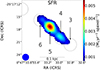 |
Fig. 11. SFR of the inner regions of NGC 253’s CMZ as accounted from the H40α RRL. The original ALCHEMI beam of 1 |

To contextualize our results, we compared our SED-based estimates (GalaPy; Table 5) with those derived from the H40α line in Bendo et al. (2015) with observations at a similar resolution. While our aperture is larger than theirs (see their Fig. 1, leftmost panel), the regions are comparable: their West, Central, and East regions correspond to our GMCs 4, 5, and 6, respectively. The SFRs derived from the H40α line in Bendo et al. (2015) (their Table 1) are on average between 6% (total H40α) and 25% (free-free corrected) lower than the ones derived by GalaPy, and this can be due to our larger apertures.
Eliminating the effect of different aperture sizes by taking the total emission in NGC 253’s CMZ, we conciliate the results: Bendo et al. (2015) reported a total SFR of 1.73 ± 0.12 M⊙ yr−1 for NGC 253’s CMZ within a 20 × 10 arcsec region. A separate 9″-radius SED (GalaPy) analysis (including Herschel PACS data) encompassing GMCs 4–6 (Fig. E.1, bottom inset in the left panel) yields a SFR of  . Including the contribution from GMCs 3 (
 ) and 7 (
 ), which also fall within the mentioned region, the total SFR raises to
  , consistent with Bendo et al. (2015)’s (free-free) value within uncertainties.
Since the H40α line is only detectable in the inner regions of the studied CMZ, at SFRs larger than about 0.870 M⊙ yr−1 (GalaPy) or 0.262 M⊙ yr−1 (CIGALE), considering GMC 3’s SFR as the lower limit, we wanted to probe its derived SFR at spaxel levels. With that aim, we decided to consider the EVLA Ka band, at 32.8 GHz, which is the band that better correlates with our SED analysis, as we will see in the next subsection (Section 4.3.3). To derive the SFR from that band, we applied the best-fit from the linear regression labeled in Fig. 13 upper panels, which for the case of the mentioned band is:
![Mathematical equation: $$ \begin{aligned} \mathrm {SFR}_{\mathrm {SED}} [M_{\odot }\ \mathrm{yr} ^{-1}] = L_{32.8\ \mathrm{GHz} }^{1.06}\ [\mathrm {erg\,s}^{-1}\,Hz^{-1} ] \cdot 10^{-29.27}, \end{aligned} $$](/articles/aa/full_html/2025/07/aa53897-25/aa53897-25-eq131.gif) (6)
(6)
in linear scale. The resulting SFR value is what we used in the y-axis of Fig. 12; whereas on the x-axis, we plot the same values as shown in Fig. 11.
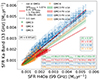 |
Fig. 12. Star formation rate (SFR) of the inner regions of NGC 253’s CMZ. In the x-axis, the SFR is obtained from the H40α RRL (see Subsect. 4.3.2). In the y-axis, the SFR was obtained from the Ka EVLA band, applying the best-fitting relation from our linear regression, presented in Eq. (6). The resulting fit considering all data points (all) and per GMC (color-coded) are labeled along with the Pearson correlation coefficient, ⟨R⟩. All points include 10% uncertainties, with regression handling errors in both axes via Markov Chain Monte Carlo, as described in our Subsect. 4.2.3. |
Figure 12 shows a variety of fits, the best fit found considering all spaxels is shown as a solid red line while the best-fitting values per GMCs are color-coded. In general, the correlations are very strong, with the largest Pearson correlation coefficient (⟨R⟩) and the closest slope to unity found for GMC 5. Taking the dashed black line, which denotes a 1:1 correspondence (“corr.” in the Fig.), as a reference, we find that the H40α derived SFR tends to be slightly overestimated in GMC 5 and slightly underestimated in the other GMCs. In general, the correlation is strong (⟨R⟩ = 0.97) and the values tend to be slightly lower than the derived ones from the 33 GHz band, with a general slope of 1.07 ± 0.01.
We note that GalaPy measures the instantaneous SFR, whereas RRLs trace star formation over the last ∼5–10 Myr (Scoville & Murchikova 2013; Emig et al. 2020). The tight correlation between the Ka-band and H40α SFRs (Figure 12) suggests that both tracers reliably probe recent star formationactivity, and that the comprised timescales should be similar.
4.3.3. Radio cm continuum and FIR
As summarized in Murphy et al. (2011), there are several SFR tracers in the wavelength range considered in this work. According to these authors, the 33 GHz continuum emission is a reliable indicator of current star formation, as it primarily arises from thermal free-free emission. Although this frequency can sometimes be affected by rotating dust, this is not the case for NGC 253 at the studied scales, as shown in the SEDs. We indeed find a strong correlation between the emission in the EVLA Ka band, as originally published in Kepley et al. (2011), and the total SFR computed by GalaPy. Furthermore, accounting for scaling offsets, we also observe generally good correlations (close to a 1:1 correspondence) between cm tracers and the GalaPy results, as seen in Fig. 13. The latter was obtained using the same approach as for the 33 GHz data, namely, by performing a linear regression in logarithmic space with all retrieved (E)VLA continuum images that detect at least four GMCs (see Table 2), aiming to obtain the best-fit assembly valid for the GMCs in the starburst galaxy NGC 253. A caveat should be noted, as different galaxy types (e.g., MW-like, dwarf galaxies, AGN hosts) may present different relationships. In this regard, an immediate prospect for the current work is to evaluate the different relations between SFR tracers.
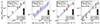 |
Fig. 13. SFR from our SED fitting using GalaPy versus fluxes from our retrieved (E)VLA continuum images, using apertures of 3″ in available GMCs (see Table 2). Best-fit linear regressions in the logarithmic scale are indicated in the top leftmost corners of each subplot, this best-fit is indicated with a dashed red line. The 1σ dispersion from the best fit to the different measurements is indicated in the bottom right corners of each subplot and also as shaded blue areas around the linear regression. (E)VLA band names are labeled with black background legends. GMCs are numbered and also color-coded following legend in Fig. D.1. We assume a conservative 10% flux uncertainty for (E)VLA observations. |
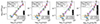 |
Fig. 14. Same as in Fig. 13, but using IR SED fitting values, both from monochromatic fluxes (at 24, 60, and 100 μm) and from integrating the total infrared luminosity range (LIR; 8–1000 μm). GMCs are numbered and also color-coded following the legend in Fig. D.1. |
Accounting for IR points as SFR tracers, as can be seen in Fig. 14, we generally find a comparable dispersion and quality of fit (in terms of mean R) to that obtained with radio bands. However, it is important to note that, since these IR data points are directly derived from the GalaPy SED fitting employed to estimate the SFR, they are not entirely independent of the latter. On the other hand, while the flux uncertainties (along the x-axis) associated with the IR data are considerably larger than those of the radio bands, this is compensated by the availability of IR points for all ten GMCs. Notwithstanding this potential interdependence, the general conclusion drawn from the IR tracers is that the best ones correspond to the integrated IR emission between 8 and 1000 μm, commonly referred to as total IR emission, and the IR emission at 60 μm.
For the radio bands, unlike optical lines, we do not assume a relation factor a priori, we only convert our mJy measurements to erg s−1 Hz−1 for an easy comparison between this study and the literature. For the mJy to erg s−1 Hz−1 conversion we have assumed a distance of 3.5 Mpc to NGC 253 (Rekola et al. 2005). For the IR bands, we retained the original units of mJy or mJy Å to allow for straightforward comparison with other studies.
5. Discussion
5.1. Reliability of our SED model along the FIR window
One of the critical, if not the most critical, challenges that astronomers have to face when attempting to fit a panchromatic SED at high angular resolution is the impossibility to acquire far infrared (FIR) observations at resolutions below 6″. Current facilities in the regime, such as the James Webb (JWST) and Euclid telescopes, cover mainly the near-IR and mid-IR parts of the electromagnetic spectrum, with the largest wavelength window ranging from 0.5 (Euclid) to 28 μm (JWST). Indeed, only the JWST can keep angular resolutions below ∼0.8″ at 28 μm. However, the FIR bump primarily occurs at wavelengths larger than those, mainly from about 50 to 300 μm.
While we made use of our well covered sub-mm regime, with ALCHEMI data, to finetune the Rayleigh-Jeans tail, at the emergence of the FIR bump on the radio side. We also used VLT/NACO data at 11 and 18.7 μm on the MIR side for GMCs 3–7, we are aware of the caveat that it is likely not enough to properly ensure the fit on the IR bump itself by solely relying on our SED model extrapolations. This is why we further retrieved archival Herschel PACS observations selecting level 2.5 PACS images at 70, 100, and 160 μm. While these FIR observations are not sufficient to resolve the targeted GMCs, they are sufficient to fit emission from the inner part of the CMZ, covering at most GMCs 3 to 6 in the worst-case scenario (at 11.3″), and partially covering GMCs 4 to 6 at 6 and 9″ (see Appendix E for more information on the latter).
In Fig. E.1, it can be noted that the far infrared peak agrees between the 3″ aperture SED, devoid of FIR photometric points and the SED at 9″, whose diffuse dust temperature, TDD, of 68.8 K is in agreement to the ones of the covered GMCs (GMCs 4–6), as noted in Table 5. Specifically, we get TDD estimations of 84.5
 , 67.9
 , and 63.3
 K for GMCs 4, 5, and 6, respectively. All in all, this arguments in favor of our 3″ apertures as the FIR bump and the SED shape in general peak at a very similar point. It is worth noting that the SED shape is responsible for sSFR estimates and, thus, for the stellar mass and SFR estimates as well (Conroy 2013).
Given the lack of FIR photometric points in the FIR regime at 3″, our SED models experienced considerable freedom in this specific wavelength range. We found that GalaPy produced SED shapes that were closer, compared to CIGALE’s models, to those observed at 9″, where Herschel PACS observations are available. Nevertheless, it is worth emphasizing that CIGALE performs well in fitting the SED of GMC 5 at 9″ (which also includes GMCs 4 and 6), both with and without an AGN component, as discussed in Appendix A.
5.2. Comparison to high-z dusty starbursts
The question of whether local starbursts can serve as analogues of primeval dusty galaxies at high redshifts (z > 4 − 8) remains a topic of active debate. A useful parameter in this context is the dust-to-stellar mass ratio, which provides insight into the balance between dust production and destructive processes such as supernova-driven shocks and astration (Nanni et al. 2020; Donevski et al. 2020; Kokorev et al. 2021; Donevski et al. 2023; Witstok et al. 2023; Palla et al. 2024; Sawant et al. 2025).
To place the ISM conditions of NGC 253 into perspective against those of distant dusty galaxies, we compare the dust-to-stellar mass ratios (Mdust/M⋆) derived in this work to those inferred from ALMA observations of high-z starbursts (Donevski et al. 2020; Salak et al. 2024; Sawant et al. 2025). Regardless of the SED fitting code used, all GMCs in NGC 253 exhibit relatively high dust-to-stellar mass ratios, with a median value of log(Mdust/M⋆) = − 2.32 ± 0.29 (values from CIGALE), or log(Mdust/M⋆) = − 2.89 ± 0.45, if values from GalaPy are considered. These ratios are close to those observed in young dusty starburst galaxies in the distant Universe. Specifically, the average dust-to-stellar mass ratio is log(Mdust/M⋆) = − 2.13 ± 0.3 at z ∼ 2 − 5 (Donevski et al. 2020) and log(Mdust/M⋆) = − 2.58 ± 0.4 at z ∼ 4 − 6 (Sawant et al. 2025). A caveat in comparing the dust-to-stellar mass ratio found here with literature is in the method used to derive galaxy properties. Both in Donevski et al. (2020) and Sawant et al. (2025), the SED fitting is performed using CIGALE, which results in average lower values with respect to GalaPy, as also reported above.
Moreover, inferred attenuation values in the GMCs of NGC 253 are comparable to those observed in high-z dusty starbursts but also significantly higher than those typically found in JWST-detected galaxies at z > 6 − 8 (e.g., Nanni et al. 2020; Álvarez-Márquez et al. 2023; Markov et al. 2025). It is important to note that, despite their comparable “dustiness”, GMCs in NGC 253 have M⋆, SFR and sSFR several orders of magnitude lower than their high-z counterparts. In such low stellar mass regimes, dust production is generally expected to be dominated solely by stellar sources, such as Type II supernovae (Galliano et al. 2018; Sommovigo et al. 2020).
However, recent models suggest that dust production in young starbursts may be significantly diminished due to ISM removal in the presence of strong stellar outflows, similar to those observed in NGC 253. To reconcile the high dust-to-stellar mass ratios, these models propose efficient growth of large dust grains through ISM accretion in rapidly cooling gas within stellar outflows (Hirashita & Chen 2023; Donevski et al. 2023; Romano et al. 2024; Palla et al. 2024). While a detailed exploration of this intriguing possibility lies beyond the scope of this work, we note that the high dust-to-stellar mass ratios and attenuations observed in the GMCs may signal that NGC 253 is undergoing a shift in the dominant dust production mechanisms, as proposed by recent simulations (see e.g., Narayanan et al. 2025, also Schneider & Maiolino 2024 for a review).
6. Conclusions and prospects
This study represents a significant step forward in understanding the CMZ of NGC 253, utilizing the first panchromatic SED analysis at a 51-pc resolution toward extragalactic regions. The integration of diverse modeling approaches, from GalaPy to CIGALE and STARLIGHT on the stellar continuum features, enabled a thorough characterization of physical properties such as SFRs, dust and stellar masses, and attenuation effects across ten GMCs using both parametric and non-parametric models.
The integration of multiwavelength SED modeling tools, such as GalaPy and CIGALE plus the integration of mono-wavelength tracers in the optical using STARLIGHT and the sub-mm using ALMA observations, provided detailed insights into star formation histories, attenuation, and stellar population properties at different timescales. High extinction values (e.g., AV exceeding 5 magnitudes in internal GMCs) were robustly derived, aligning well with other methods and showcasing the importance of panchromatic approaches. We summarize our main findings below.
-
Dynamical and chemical diversity: The CMZ of NGC 253 exhibits significant dynamical and chemical distinctions between internal (nuclear) and external GMCs. Internal GMCs (e.g., GMCs 3–6) are characterized by higher SFRs, stellar masses, and dust masses, consistent with active star formation, high-excitation regions, and higher metallicities. External GMCs (e.g., GMCs 1, 2, 7–10) display lower density, slower and weaker shocks, and chemical signatures indicative of less energetic processes as compared to the internal GMCs.
-
Comparison of internal versus external GMCs: Internal GMCs exhibit stellar masses in the range of
 –
– and dust masses in the range of
  –
– , both greatly surpassing (even doubling) the maximum values observed in external GMCs. The sSFR results further underscore these differences, exhibiting a trend of enhanced values in the nuclear regions.
 -
Insights from age-metallicity relations: Differences in stellar ages and metallicities highlight the varied evolutionary states of the studied GMCs. Depending on the adopted software, these values can vary by up to two orders of magnitude in age (STARLIGHT; Table 7) and one order of magnitude in metallicity (GalaPy; Table 5).
-
Emission line diagnostics: The BPT and WHAN diagrams indicate shock signatures in the nuclear region of NGC 253, placing it in the composite zone. However, these shocks likely result from stellar winds and supernovae in the starburst environment and not from AGN activity.
-
Caveats on Hα’s derived SFR: While Hα remains a popular SFR tracer, our analysis reveals its significant limitations in NGC 253’s dust-obscured CMZ, where attenuation causes large discrepancies compared to more robust radio (e.g., the band at 33 GHz) and panchromatic SED tracers. This suggests that Hα should be supplemented with dust-insensitive indicators in similar environments.
-
Star formation, panchromatic versus monochromatic results: We have found a strong 1:1 correlation between cm tracers and SED derived SFR values, with the Ka-band (at 33 GHz) found to be the best among the available dataset. This is in line with previous works based on entire galaxy properties (e.g., Murphy et al. 2011) and is now confirmed at GMC scales. Additionally, we validate the effectiveness of RRLs (H40α) as a SF tracer, although it is limited to the brightest sources (GMCs 3–6).
The current study provides a robust framework for leveraging spatially resolved multiwavelength datasets to investigate the interplay between star formation, gas dynamics, and attenuation in starburst galaxies. In addition, this work not only advances our knowledge of starburst environments but also serves as a benchmark for studying high-redshift galaxies, where similar extreme conditions prevail.
In the future, we plan to focus on several key directions to broaden the applicability of these findings. These include utilizing JWST instead of Spitzer observations, achieving aperture diameters as fine as 1″ in the mid-IR, enabling more detailed analyses of star-forming regions and/or augmenting the redshift regime for our potential targets. We plan to apply the same approach to other well-known starburst such as M 82. Alternatively, we want to improve the robustness of our fit by restricting ourselves to very nearby galaxies where FIR data from Herschel can still resolve GMC-scale structures; that is, if we assume a GMC size of 50 pc, and a Herschel aperture of 9″, we can utilize Herschel/PACS FIR observations of Milky Way’s and Andromeda’s satellites, yielding approximately 20 objects.
Additionally, this framework has the potential to be extended to diverse systems, including Milky Way-like galaxies, LINERs, ULIRGs, and AGN, to explore differences in star formation processes across various galactic environments. Furthermore, focused studies of GMCs in our Galaxy will offer a critical baseline for contrasting extragalactic GMC properties, contributing to a thorough understanding of star formation under varying conditions. As a final remark, we also aim to provide future GalaPy users with a full set of priors that are well suited for GMC scales in extreme, intensively star-forming and highly obscured environments. This will also be helpful in studies of Galactic analogues such as Sgr B2 mini-starbursting system (Belloche et al. 2013; Schwörer et al. 2019) and the distant (high-z) universe.
The Strehl ratio (SR) is a measure of the quality of adaptive optics correction, indicating the ratio of the peak intensity of the observed point spread function to the ideal diffraction-limited one.
According to the smaller array extension of the hybrid configuration, configuration C for this case.
Acknowledgments
We thank the anonymous referee for their helpful comments, questions, and suggestions on revising the manuscript. P.K.H. gratefully acknowledges the Fundação de Amparo à Pesquisa do Estado de São Paulo (FAPESP) for the support grant 2023/14272-4. P.K.H. acknowledges L. Barcos for discussions on the project’s initial scope, E. Caux for insights into the FIR cross-validation methodology, G. Ortiz-León for support with the EVLA X-band data reduction, and D. Hazarika for guidance on the proper implementation of the MCMC algorithm for the linear regression analysis. We thank A. Kepley for providing us with the 33 GHz (Ka-band) EVLA image. S.D has been supported by the Polish National Science Center project UMO-2023/51/D/ST9/00147 TR is supported by the Italian Research Center on High Performance Computing Big Data and Quantum Computing (ICSC), project funded by European Union – NextGenerationEU – and National Recovery and Resilience Plan (NRRP) – Mission 4 Component 2 within the activities of Spoke 3 (Astrophysics and Cosmos Observations). D.D. acknowledges support from the National Science Center (NCN) grant SONATA (UMO-2020/39/D/ST9/00720). JAFO acknowledges financial support by the Spanish Ministry of Science and Innovation (MCIN/AEI/10.13039/501100011033), by “ERDF A way of making Europe” and by “European Union NextGenerationEU/PRTR” through the grants PID2021-124918NB-C44 and CNS2023-145339; MCIN and the European Union – NextGenerationEU through the Recovery and Resilience Facility project ICTS-MRR-2021-03-CEFCA. M.H. acknowledges the support by the National Science Centre, Poland (UMO-2022/45/N/ST9/01336). V.M.R. and L.C. acknowledge support from the grant PID2022-136814NB-I00 by the Spanish Ministry of Science, Innovation and Universities/State Agency of Research MICIU/AEI/10.13039/501100011033 and by ERDF, UE. V.M.R also acknowledges support from the grant RYC2020-029387-I funded by MICIU/AEI/10.13039/501100011033 and by “ESF, Investing in your future”, and from the Consejo Superior de Investigaciones Científicas (CSIC) and the Centro de Astrobiología (CAB) through the project 20225AT015 (Proyectos intramurales especiales del CSIC); and from the grant CNS2023-144464 funded by MICIU/AEI/10.13039/501100011033 and by “European Union NextGenerationEU/PRTR”. A.R.L. acknowledges financial support from Consejo Nacional de Investigaciones Científicas y Técnicas (CONICET), Agencia I+D+i (PICT 2019–03299) and Universidad Nacional de La Plata (Argentina). A.C.K thanks Fundação de Amparo à Pesquisa do Estado de São Paulo (FAPESP) for the support grant 2024/05467-9. SP is supported by the international Gemini Observatory, a program of NSF NOIRLab, which is managed by the Association of Universities for Research in Astronomy (AURA) under a cooperative agreement with the U.S. National Science Foundation, on behalf of the Gemini partnership of Argentina, Brazil, Canada, Chile, the Republic of Korea, and the United States of America. R.D. gratefully acknowledges support by the ANID BASAL project FB210003 For the near-UV, optical, and near-IR regimes, this work utilizes data from the S-PLUS collaboration (Mendes de Oliveira et al. 2019), as well as VLT and HST observations reported by Fernández-Ontiveros et al. (2009). Additionally, this study is partially based on archival data obtained with the Spitzer Space Telescope, which was operated by the Jet Propulsion Laboratory, California Institute of Technology, under a contract with NASA. For radio observations, this work includes the following ALMA data: : ADS/JAO.ALMA#2017.1.00161.L and ADS/JAO.ALMA#2018.1.00162.S. ALMA is a partnership of ESO (representing its member states), NSF (USA) and NINS (Japan), together with NRC (Canada), MOST and ASIAA (Taiwan), and KASI (Republic of Korea), in cooperation with the Republic of Chile. The Joint ALMA Observatory is operated by ESO, AUI/NRAO and NAOJ. This study also made use of (extended) Karl G. Jansky Very Large Array archival observations provided by the National Radio Astronomy Observatory (NRAO), a facility of the National Science Foundation operated under cooperative agreement by Associated Universities, Inc. In constructing the SED fitting at 9″ resolution, this work incorporates observations from the ESA Herschel Space Observatory (Pilbratt et al. 2010), specifically using the PACS instrument (Poglitsch et al. 2010).
References
- Allard, E. L., Peletier, R. F., & Knapen, J. H. 2005, ApJ, 633, L25 [NASA ADS] [CrossRef] [Google Scholar]
- Allard, E. L., Knapen, J. H., Peletier, R. F., & Sarzi, M. 2006, MNRAS, 371, 1087 [CrossRef] [Google Scholar]
- Álvarez-Márquez, J., Crespo Gómez, A., Colina, L., et al. 2023, A&A, 671, A105 [NASA ADS] [CrossRef] [EDP Sciences] [Google Scholar]
- Anantharamaiah, K. R., & Goss, W. M. 1996, ApJ, 466, L13 [NASA ADS] [CrossRef] [Google Scholar]
- Ando, R., Nakanishi, K., Kohno, K., et al. 2017, ApJ, 849, 81 [CrossRef] [Google Scholar]
- Baes, M., Verstappen, J., De Looze, I., et al. 2011, ApJS, 196, 22 [Google Scholar]
- Baldwin, J. A., Phillips, M. M., & Terlevich, R. 1981, PASP, 93, 5 [Google Scholar]
- Bao, M., Harada, N., Kohno, K., et al. 2024, A&A, 687, A43 [NASA ADS] [CrossRef] [EDP Sciences] [Google Scholar]
- Beck, A., Lebouteiller, V., Madden, S. C., et al. 2022, A&A, 665, A85 [NASA ADS] [CrossRef] [EDP Sciences] [Google Scholar]
- Behrens, E., Mangum, J. G., Holdship, J., et al. 2022, ApJ, 939, 119 [NASA ADS] [CrossRef] [Google Scholar]
- Behrens, E., Mangum, J. G., Viti, S., et al. 2024, ApJ, 977, 38 [Google Scholar]
- Belfiori, D., Paladino, R., Hughes, A., et al. 2025, A&A, 697, A24 [NASA ADS] [CrossRef] [EDP Sciences] [Google Scholar]
- Belloche, A., Müller, H. S. P., Menten, K. M., Schilke, P., & Comito, C. 2013, A&A, 559, A47 [NASA ADS] [CrossRef] [EDP Sciences] [Google Scholar]
- Bendo, G. J., Beswick, R. J., D’Cruze, M. J., et al. 2015, MNRAS, 450, L80 [NASA ADS] [CrossRef] [Google Scholar]
- Boquien, M., Burgarella, D., Roehlly, Y., et al. 2019, A&A, 622, A103 [NASA ADS] [CrossRef] [EDP Sciences] [Google Scholar]
- Bouvier, M., Viti, S., Behrens, E., et al. 2024, A&A, 689, A64 [NASA ADS] [CrossRef] [EDP Sciences] [Google Scholar]
- Bressan, A., Silva, L., & Granato, G. L. 2002, A&A, 392, 377 [NASA ADS] [CrossRef] [EDP Sciences] [Google Scholar]
- Bressan, A., Marigo, P., Girardi, L., et al. 2012, MNRAS, 427, 127 [NASA ADS] [CrossRef] [Google Scholar]
- Brunthaler, A., Castangia, P., Tarchi, A., et al. 2009, A&A, 497, 103 [NASA ADS] [CrossRef] [EDP Sciences] [Google Scholar]
- Bruzual, G., & Charlot, S. 2003, MNRAS, 344, 1000 [NASA ADS] [CrossRef] [Google Scholar]
- Bulatek, A., Ginsburg, A., Darling, J., Henkel, C., & Menten, K. M. 2023, ApJ, 956, 78 [Google Scholar]
- Butterworth, J., Viti, S., Van der Werf, P. P., et al. 2024, A&A, 686, A31 [NASA ADS] [CrossRef] [EDP Sciences] [Google Scholar]
- Calzetti, D., Armus, L., Bohlin, R. C., et al. 2000, ApJ, 533, 682 [NASA ADS] [CrossRef] [Google Scholar]
- Cardelli, J. A., Clayton, G. C., & Mathis, J. S. 1989, ApJ, 345, 245 [Google Scholar]
- Chabrier, G. 2003, PASP, 115, 763 [Google Scholar]
- Charlot, S., & Fall, S. M. 2000, ApJ, 539, 718 [Google Scholar]
- Chen, Y., Bressan, A., Girardi, L., et al. 2015, MNRAS, 452, 1068 [Google Scholar]
- Chevance, M., Kruijssen, J. M. D., Hygate, A. P. S., et al. 2020, MNRAS, 493, 2872 [NASA ADS] [CrossRef] [Google Scholar]
- Cid Fernandes, R., Mateus, A., Sodré, L., Stasińska, G., & Gomes, J. M. 2005, MNRAS, 358, 363 [Google Scholar]
- Cid Fernandes, R., Stasińska, G., Schlickmann, M. S., et al. 2010, MNRAS, 403, 1036 [Google Scholar]
- Cid Fernandes, R., Pérez, E., García Benito, R., et al. 2013, A&A, 557, A86 [NASA ADS] [CrossRef] [EDP Sciences] [Google Scholar]
- Ciesla, L., Charmandaris, V., Georgakakis, A., et al. 2015, A&A, 576, A10 [NASA ADS] [CrossRef] [EDP Sciences] [Google Scholar]
- Clemens, M. S., Scaife, A., Vega, O., & Bressan, A. 2010, MNRAS, 405, 887 [NASA ADS] [Google Scholar]
- Cohen, D. P., Turner, J. L., & Consiglio, S. M. 2020, MNRAS, 493, 627 [NASA ADS] [CrossRef] [Google Scholar]
- Condon, J. J., Huang, Z. P., Yin, Q. F., & Thuan, T. X. 1991, ApJ, 378, 65 [Google Scholar]
- Conroy, C. 2013, ARA&A, 51, 393 [NASA ADS] [CrossRef] [Google Scholar]
- da Cunha, E., Charlot, S., & Elbaz, D. 2008, MNRAS, 388, 1595 [Google Scholar]
- Dey, S., Goyal, A., Małek, K., et al. 2022, ApJ, 938, 152 [NASA ADS] [CrossRef] [Google Scholar]
- Dey, S., Goyal, A., Małek, K., & Díaz-Santos, T. 2024, ApJ, 966, 61 [Google Scholar]
- Donevski, D., Lapi, A., Małek, K., et al. 2020, A&A, 644, A144 [NASA ADS] [CrossRef] [EDP Sciences] [Google Scholar]
- Donevski, D., Damjanov, I., Nanni, A., et al. 2023, A&A, 678, A35 [NASA ADS] [CrossRef] [EDP Sciences] [Google Scholar]
- Draine, B. T., Aniano, G., Krause, O., et al. 2014, ApJ, 780, 172 [Google Scholar]
- Ellingsen, S. P., Chen, X., Breen, S. L., & Qiao, H. H. 2017, MNRAS, 472, 604 [NASA ADS] [CrossRef] [Google Scholar]
- Emig, K. L., Bolatto, A. D., Leroy, A. K., et al. 2020, ApJ, 903, 50 [NASA ADS] [CrossRef] [Google Scholar]
- Fazio, G. G., Hora, J. L., Allen, L. E., et al. 2004, ApJS, 154, 10 [Google Scholar]
- Fernández-Ontiveros, J. A., Prieto, M. A., & Acosta-Pulido, J. A. 2009, MNRAS, 392, L16 [CrossRef] [Google Scholar]
- Foreman-Mackey, D., Hogg, D. W., Lang, D., & Goodman, J. 2013, PASP, 125, 306 [Google Scholar]
- Galliano, F., Galametz, M., & Jones, A. P. 2018, ARA&A, 56, 673 [Google Scholar]
- Galvin, T. J., Seymour, N., Marvil, J., et al. 2018, MNRAS, 474, 779 [Google Scholar]
- Gentile, F., Talia, M., Daddi, E., et al. 2024, A&A, 687, A288 [NASA ADS] [CrossRef] [EDP Sciences] [Google Scholar]
- Giulietti, M., Lapi, A., Massardi, M., et al. 2023, ApJ, 943, 151 [NASA ADS] [CrossRef] [Google Scholar]
- Gommers, R., Virtanen, P., Haberland, M., et al. 2025, https://doi.org/10.5281/zenodo.595738 [Google Scholar]
- Gorski, M. D., Ott, J., Rand, R., et al. 2019, MNRAS, 483, 5434 [NASA ADS] [CrossRef] [Google Scholar]
- Hamed, M., Ciesla, L., Béthermin, M., et al. 2021, A&A, 646, A127 [NASA ADS] [CrossRef] [EDP Sciences] [Google Scholar]
- Hamed, M., Małek, K., Buat, V., et al. 2023, A&A, 674, A99 [NASA ADS] [CrossRef] [EDP Sciences] [Google Scholar]
- Harada, N., Martín, S., Mangum, J. G., et al. 2021, ApJ, 923, 24 [NASA ADS] [CrossRef] [Google Scholar]
- Harada, N., Martín, S., Mangum, J. G., et al. 2022, ApJ, 938, 80 [NASA ADS] [CrossRef] [Google Scholar]
- Harada, N., Meier, D. S., Martín, S., et al. 2024, ApJS, 271, 38 [NASA ADS] [CrossRef] [Google Scholar]
- Hernández-Gómez, A., Sahnoun, E., Caux, E., et al. 2019, MNRAS, 483, 2014 [CrossRef] [Google Scholar]
- Herpich, F. R., Almeida-Fernandes, F., Oliveira Schwarz, G. B., et al. 2024, A&A, 689, A249 [NASA ADS] [CrossRef] [EDP Sciences] [Google Scholar]
- Hirashita, H., & Chen, C.-C. 2023, MNRAS, 526, 4710 [Google Scholar]
- Holdship, J., Viti, S., Martín, S., et al. 2021, A&A, 654, A55 [NASA ADS] [CrossRef] [EDP Sciences] [Google Scholar]
- Holdship, J., Mangum, J. G., Viti, S., et al. 2022, ApJ, 931, 89 [NASA ADS] [CrossRef] [Google Scholar]
- Hopkins, A. M., & Beacom, J. F. 2006, ApJ, 651, 142 [NASA ADS] [CrossRef] [Google Scholar]
- Hopkins, P. F., Bundy, K., Croton, D., et al. 2010, ApJ, 715, 202 [Google Scholar]
- Huang, K. Y., Viti, S., Holdship, J., et al. 2023, A&A, 675, A151 [NASA ADS] [CrossRef] [EDP Sciences] [Google Scholar]
- Humire, P. K., Thiel, V., Henkel, C., et al. 2020, A&A, 642, A222 [NASA ADS] [CrossRef] [EDP Sciences] [Google Scholar]
- Humire, P. K., Henkel, C., Hernández-Gómez, A., et al. 2022, A&A, 663, A33 [NASA ADS] [CrossRef] [EDP Sciences] [Google Scholar]
- Humire, P. K., Ortiz-León, G. N., Hernández-Gómez, A., et al. 2024, A&A, 688, L1 [NASA ADS] [CrossRef] [EDP Sciences] [Google Scholar]
- Iodice, E., Arnaboldi, M., Rejkuba, M., et al. 2014, A&A, 567, A86 [NASA ADS] [CrossRef] [EDP Sciences] [Google Scholar]
- Kapińska, A. D., Staveley-Smith, L., Crocker, R., et al. 2017, ApJ, 838, 68 [CrossRef] [Google Scholar]
- Kauffmann, G., Heckman, T. M., Tremonti, C., et al. 2003, MNRAS, 346, 1055 [Google Scholar]
- Kellermann, K. I., & Pauliny-Toth, I. I. K. 1969, ApJ, 155, L71 [NASA ADS] [CrossRef] [Google Scholar]
- Kennicutt, R. C., Jr 1998, ARA&A, 36, 189 [NASA ADS] [CrossRef] [Google Scholar]
- Kepley, A. A., Chomiuk, L., Johnson, K. E., et al. 2011, ApJ, 739, L24 [CrossRef] [Google Scholar]
- Kewley, L. J., Dopita, M. A., Sutherland, R. S., Heisler, C. A., & Trevena, J. 2001a, ApJ, 556, 121 [Google Scholar]
- Kewley, L. J., Heisler, C. A., Dopita, M. A., & Lumsden, S. 2001b, ApJS, 132, 37 [Google Scholar]
- Kim, W.-T., Seo, W.-Y., & Kim, Y. 2012, ApJ, 758, 14 [NASA ADS] [CrossRef] [Google Scholar]
- Kobayashi, C., Karakas, A. I., & Umeda, H. 2011, MNRAS, 414, 3231 [Google Scholar]
- Kobayashi, C., Karakas, A. I., & Lugaro, M. 2020, ApJ, 900, 179 [Google Scholar]
- Kokorev, V. I., Magdis, G. E., Davidzon, I., et al. 2021, ApJ, 921, 40 [NASA ADS] [CrossRef] [Google Scholar]
- Krabbe, A. C., Rosa, D. A., Pastoriza, M. G., et al. 2017, MNRAS, 467, 27 [NASA ADS] [CrossRef] [Google Scholar]
- Kruijssen, J. M. D., & Longmore, S. N. 2014, MNRAS, 439, 3239 [NASA ADS] [CrossRef] [Google Scholar]
- Lapi, A., Pantoni, L., Zanisi, L., et al. 2018, ApJ, 857, 22 [NASA ADS] [CrossRef] [Google Scholar]
- Lapi, A., Pantoni, L., Boco, L., & Danese, L. 2020, ApJ, 897, 81 [NASA ADS] [CrossRef] [Google Scholar]
- Leroy, A. K., Bolatto, A. D., Ostriker, E. C., et al. 2015, ApJ, 801, 25 [NASA ADS] [CrossRef] [Google Scholar]
- Li, N., & Li, C. 2024, ApJ, 975, 234 [Google Scholar]
- López Fernández, R., Cid Fernandes, R., González Delgado, R. M., et al. 2016, MNRAS, 458, 184 [CrossRef] [Google Scholar]
- Mangum, J. G., Ginsburg, A. G., Henkel, C., et al. 2019, ApJ, 871, 170 [NASA ADS] [CrossRef] [Google Scholar]
- Markov, V., Gallerani, S., Ferrara, A., et al. 2025, Nat. Astron., 9, 458 [Google Scholar]
- Martín, S., Mangum, J. G., Harada, N., et al. 2021, A&A, 656, A46 [NASA ADS] [CrossRef] [EDP Sciences] [Google Scholar]
- Martínez-Paredes, M., Bruzual, G., Morisset, C., et al. 2023, MNRAS, 525, 2916 [CrossRef] [Google Scholar]
- Meier, D. S., Walter, F., Bolatto, A. D., et al. 2015, ApJ, 801, 63 [NASA ADS] [CrossRef] [Google Scholar]
- Mendes de Oliveira, C., Ribeiro, T., Schoenell, W., et al. 2019, MNRAS, 489, 241 [NASA ADS] [CrossRef] [Google Scholar]
- Müller, H. S. P., Schlöder, F., Stutzki, J., & Winnewisser, G. 2005, J. Mol. Struct., 742, 215 [Google Scholar]
- Müller-Sánchez, F., González-Martín, O., Fernández-Ontiveros, J. A., Acosta-Pulido, J. A., & Prieto, M. A. 2010, ApJ, 716, 1166 [CrossRef] [Google Scholar]
- Murphy, E. J., Condon, J. J., Schinnerer, E., et al. 2011, ApJ, 737, 67 [Google Scholar]
- Nanni, A., Burgarella, D., Theulé, P., Côté, B., & Hirashita, H. 2020, A&A, 641, A168 [NASA ADS] [CrossRef] [EDP Sciences] [Google Scholar]
- Narayanan, D., Stark, D. P., Finkelstein, S. L., et al. 2025, ApJ, 982, 7 [Google Scholar]
- Osterbrock, D. E., & Ferland, G. J. 2006, Astrophysics of Gaseous Nebulae and Active Galactic Nuclei (Sausalito, CA: University Science Books) [Google Scholar]
- Palla, M., De Looze, I., Relaño, M., et al. 2024, MNRAS, 528, 2407 [NASA ADS] [CrossRef] [Google Scholar]
- Pantoni, L., Lapi, A., Massardi, M., Goswami, S., & Danese, L. 2019, ApJ, 880, 129 [NASA ADS] [CrossRef] [Google Scholar]
- Pence, W. D. 1980, ApJ, 239, 54 [NASA ADS] [CrossRef] [Google Scholar]
- Pérez-Beaupuits, J. P., Güsten, R., Harris, A., et al. 2018, ApJ, 860, 23 [Google Scholar]
- Pilbratt, G. L., Riedinger, J. R., Passvogel, T., et al. 2010, A&A, 518, L1 [NASA ADS] [CrossRef] [EDP Sciences] [Google Scholar]
- Planck Collaboration VI. 2020, A&A, 641, A6 [NASA ADS] [CrossRef] [EDP Sciences] [Google Scholar]
- Poglitsch, A., Waelkens, C., Geis, N., et al. 2010, A&A, 518, L2 [NASA ADS] [CrossRef] [EDP Sciences] [Google Scholar]
- Rekola, R., Richer, M. G., McCall, M. L., et al. 2005, MNRAS, 361, 330 [NASA ADS] [CrossRef] [Google Scholar]
- Rico-Villas, F., Martín-Pintado, J., González-Alfonso, E., Martín, S., & Rivilla, V. M. 2020, MNRAS, 491, 4573 [NASA ADS] [CrossRef] [Google Scholar]
- Romano, M., Donevski, D., Junais, et al. 2024, A&A, 683, L9 [NASA ADS] [CrossRef] [EDP Sciences] [Google Scholar]
- Ronconi, T., Lapi, A., Torsello, M., et al. 2024, A&A, 685, A161 [NASA ADS] [CrossRef] [EDP Sciences] [Google Scholar]
- Rosolowsky, E., & Leroy, A. 2006, PASP, 118, 590 [NASA ADS] [CrossRef] [Google Scholar]
- Sakamoto, K., Ho, P. T. P., Iono, D., et al. 2006, ApJ, 636, 685 [NASA ADS] [CrossRef] [Google Scholar]
- Sakamoto, K., Mao, R.-Q., Matsushita, S., et al. 2011, ApJ, 735, 19 [CrossRef] [Google Scholar]
- Salak, D., Hashimoto, T., Inoue, A. K., et al. 2024, ApJ, 962, 1 [NASA ADS] [CrossRef] [Google Scholar]
- Salim, S., & Narayanan, D. 2020, ARA&A, 58, 529 [NASA ADS] [CrossRef] [Google Scholar]
- Salpeter, E. E. 1955, ApJ, 121, 161 [Google Scholar]
- Sawant, P., Nanni, A., Romano, M., et al. 2025, A&A, 694, A82 [NASA ADS] [CrossRef] [EDP Sciences] [Google Scholar]
- Schneider, R., & Maiolino, R. 2024, A&ARv, 32, 2 [NASA ADS] [CrossRef] [Google Scholar]
- Schreiber, C., Glazebrook, K., Nanayakkara, T., et al. 2018, A&A, 618, A85 [NASA ADS] [CrossRef] [EDP Sciences] [Google Scholar]
- Schwörer, A., Sánchez-Monge, Á., Schilke, P., et al. 2019, A&A, 628, A6 [NASA ADS] [CrossRef] [EDP Sciences] [Google Scholar]
- Scoville, N., & Murchikova, L. 2013, ApJ, 779, 75 [CrossRef] [Google Scholar]
- Sommovigo, L., Ferrara, A., Pallottini, A., et al. 2020, MNRAS, 497, 956 [NASA ADS] [CrossRef] [Google Scholar]
- Stalevski, M., Fritz, J., Baes, M., Nakos, T., & Popović, L. Č. 2012, MNRAS, 420, 2756 [Google Scholar]
- Stalevski, M., Ricci, C., Ueda, Y., et al. 2016, MNRAS, 458, 2288 [Google Scholar]
- Stasińska, G., Cid Fernandes, R., Mateus, A., Sodré, L., & Asari, N. V. 2006, MNRAS, 371, 972 [Google Scholar]
- Stroe, A., Oosterloo, T., Röttgering, H. J. A., et al. 2015, MNRAS, 452, 2731 [NASA ADS] [CrossRef] [Google Scholar]
- Swinbank, A. M., Smail, I., Longmore, S., et al. 2010, Nature, 464, 733 [Google Scholar]
- Tanaka, K., Mangum, J. G., Viti, S., et al. 2024, ApJ, 961, 18 [NASA ADS] [CrossRef] [Google Scholar]
- Turner, J. L., & Ho, P. T. P. 1985, ApJ, 299, L77 [NASA ADS] [CrossRef] [Google Scholar]
- van der Tak, F. F. S., Black, J. H., Schöier, F. L., Jansen, D. J., & van Dishoeck, E. F. 2007, A&A, 468, 627 [NASA ADS] [CrossRef] [EDP Sciences] [Google Scholar]
- Vastel, C., Bottinelli, S., Caux, E., Glorian, J. M., & Boiziot, M. 2015, in SF2A-2015: Proceedings of the Annual meeting of the French Society of Astronomy and Astrophysics, 313 [Google Scholar]
- Walmsley, C. 1989, in Interstellar Dust, eds. L. J. Allamandola, & A. G. G. M. Tielens, 135, 263 [Google Scholar]
- Walter, F., Bolatto, A. D., Leroy, A. K., et al. 2017, ApJ, 835, 265 [NASA ADS] [CrossRef] [Google Scholar]
- Wenger, M., Ochsenbein, F., Egret, D., et al. 2000, A&AS, 143, 9 [NASA ADS] [CrossRef] [EDP Sciences] [Google Scholar]
- Werle, A., Cid Fernandes, R., Vale Asari, N., et al. 2019, MNRAS, 483, 2382 [Google Scholar]
- Wirström, E. S., Bergman, P., Black, J. H., et al. 2010, A&A, 522, A19 [Google Scholar]
- Witstok, J., Jones, G. C., Maiolino, R., Smit, R., & Schneider, R. 2023, MNRAS, 523, 3119 [NASA ADS] [CrossRef] [Google Scholar]
- Xiang, M., & Rix, H.-W. 2022, Nature, 603, 599 [NASA ADS] [CrossRef] [Google Scholar]
- Yan, Y. T., Zhang, J. S., Henkel, C., et al. 2019, ApJ, 877, 154 [Google Scholar]
- Yang, G., Boquien, M., Brandt, W. N., et al. 2022, ApJ, 927, 192 [NASA ADS] [CrossRef] [Google Scholar]
- Zeng, S., Zhang, Q., Jiménez-Serra, I., et al. 2020, MNRAS, 497, 4896 [NASA ADS] [CrossRef] [Google Scholar]
- Zhao, J. Y., Zhang, J. S., Wang, Y. X., et al. 2023, ApJS, 266, 29 [Google Scholar]
Appendix A: CIGALE SED modeling with AGN component
To assess potential AGN contributions, we incorporated the SKIRTOR module (Stalevski et al. 2012, 2016). SKIRTOR is based on the 3D radiative transfer code SKIRT (Baes et al. 2011). It includes obscuration by dusty torus and obscuration by dust settled along with the polar directions. The 2022.1 version of CIGALE offers significant advancements over its predecessors, particularly through its enhanced radio module, which includes both thermal (free-free emission from nebular gas) and nonthermal (synchrotron emission from star formation and AGN activity) contributions. The updated module also incorporates a new AGN component, enabling us to estimate the radio loudness, RAGN, defined as the ratio of AGN luminosities measured at 5 GHz and 2500Å. Additionally, it provides the slope of the AGN power-law (PL) radiation, which is assumed to be isotropic (Yang et al. 2022).
CIGALE 2022.1 models the radio luminosities from star formation and AGN components using the FIR/radio correlation coefficient (qIR) and radio loudness (RAGN) parameters in scaling relations. At 1.4 GHz, the radio luminosity from star formation is predominantly nonthermal synchrotron emission, normalized using the qIR parameter. The qIR determines the normalization at this frequency, while a single power-law describes the synchrotron emission from star formation. Variations in the qIR parameter contribute to uncertainties in modeling the radio component with CIGALE. The nonthermal synchrotron emission from the AGN is also described using a single PL form governed by the RAGN parameter. However, the galaxy-averaged radio SEDs of starburst galaxies are rarely represented by single-PL models, showing low-frequency turnover due to free-free absorption (e.g., Galvin et al. 2018; Dey et al. 2022, 2024). It would be interesting to compare the physical conditions responsible for radio emission on the galaxy-wide scale to GMC scales, and that will be the aim of future studies using spatially-resolved radio SEDs of NGC 253. The list of input parameters to CIGALE analysis without and with AGN component is given in Table A.1. For the CIGALE modeling including the AGN component, we only added the AGN module to the existing input parameters. These CIGALE inputs have yielded a mean reduced χ2 of 2.2 for the ten GMCs studied in this work. The resulting SEDs are shown in Figs. A.1 (without an AGN component) and A.2 (considering an AGN component). These Figs. also include, in the bottom middle panel each, the SED fitting centered at GMC 5 at 9″ aperture diameter, which allows us to include Herschel PACS observations (see Appendix E). The results on the main physical properties for each GMC are shown in Table 6, those regarding attenuation effects are also in Table A.2 while additional results can be found in Tables A.3, and A.4.
List of input parameters for CIGALE modeling.
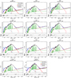 |
Fig. A.1. Best-fit CIGALE SEDs without an AGN component of the ten GMCs studied here plus a 9″ aperture SED for the nuclear region, also devoid of an AGN component, in the bottom middle panel. Open blue circles are the observed fluxes while filled red points indicate modeled fluxes whose observed values may or may not be fitted, depending on their availability (see Table 2). The goodness of fit is estimated by the reduced χ2 shown at the top of each panel, along with the name and redshift of the GMC. In almost all cases, SEDs are well modeled, giving reasonable estimates of astrophysical properties. In Fig. A.2 we show our best-fits CIGALE models considering an AGN component. |
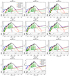 |
Fig. A.2. Best-fit CIGALE+AGN SEDs of the ten GMCs studied here plus a 9″ aperture SED for the nuclear region, also considering an AGN component, in the bottom middle panel. Open blue circles are the observed fluxes while filled red points indicate modeled fluxes whose observed values may or may not be fitted, depending on their availability (see Table 2). The goodness of fit is estimated by the reduced χ2 shown at the top of each panel, along with the name and redshift of the GMC. In almost all cases, SEDs are well modeled, giving reasonable estimates of astrophysical properties. |
The extinction-related results obtained from SED modeling with CIGALE, including the AGN component.
Dust and SFH related results obtained from SED modeling with CIGALE, including AGN component.
Results of AGN and radio SED modeling using CIGALE.
Appendix B: Individual GMC properties
GMC 1: Located at the boundaries of the CMZ, where x1/x2 interactions are present, GMC 1 traces weak shocks at low-frequency transitions (Humire et al. 2022; Harada et al. 2022; Huang et al. 2023) and strong shocks at high-J frequency transitions. Indeed, the strongest SiO(5–4)/HNCO(100, 10 − 90, 9) ratios are observed at this position (Humire et al. 2022). The whole picture may also be that weak and strong shocks are actually mixed over the entire CMZ (Bao et al. 2024). The shocked environment results in some of the more prominent Class I methanol masers (MMCIs) in the J−1 → (J− 1)0 − E and J0 → (J− 1)1 − A line series (Ellingsen et al. 2017; Gorski et al. 2019; Humire et al. 2022). Devoid of a strong continuum, but showing the strongest maser over LTE emission (Humire et al. 2022, their Fig. 13), GMC 1 appears to be an extragalactic example of what is seen in the Milky Way object GMC G+0.693 (Zeng et al. 2020). In line with the latter, this cloud possesses the lowest amount of dust and stellar masses in the sample, according to GalaPy (see Table B.1).
Contrary to the others GMCs in our sample, GMC 1 is the only one whose SED fitting could also deliver ages of the order of 105 years. However, since we observe CO emission, a molecule that needs a few million years to be produced (e.g., Walmsley 1989), a permitted range of 106 − 11 or 106 − 12 years was imposed to all GMCs. This restriction yielded SED shapes that are closer to the observed ones compared to those with an age of ∼105 years, and significantly improved the results at millimeter and centimeter wavelengths by better reproducing the observed flux densities.
Gas, star-formation (SF) related parameters and dust-related parameters for all SED results derived from GalaPy.
GMC 2: This molecular cloud also overlaps with x1/x2 interactions and presents physical and chemical conditions that are similar to GMC 1, although GMC 2 is more massive in terms of stellar and dust mass (Table B.1; see also Humire et al. 2022 and Bouvier et al. 2024), older (Table B.1), and shows weaker MMCIs exclusively in the J−1 → (J− 1)0 − E family (Humire et al. 2022). With slightly lower values than GMC 1, GMc 2 presents the lowest dusty radius, as calculated by GalaPy, and the lowest stellar mass, according to STARLIGHT, as indicated in Tables B.1 and 7, respectively.
GMC 3 appears to be the source of the stellar outflow best viewed by high-density tracers such as CN, HCN (Walter et al. 2017), or an increment in the CO/13CO J = 1–0 ratios owed to a more transparent environment (Bao et al. 2024). Although dense molecular gas possess a velocity dispersion of ∼40 km s−1 in the streamer (Walter et al. 2017), the stellar velocity dispersion is the lowest among the sample (see Table 7) at the GMC position. This corresponds to the depiction of cold/low-dispersion gas actively producing stars at the convergence of the ring and the bar, as observed in M 100 (Allard et al. 2005). A more evolved and therefore, more easily observed stellar stream is in line with this position being the oldest among the nuclear regions, as deduced from our SED fitting in Table B.1. In the same table, and also in Figure4, it can be seen than GMC 3 presents the largest dust reservoir and extension.
GMC 4 exhibits the highest SiO(2–1)/HNCO(40, 4 − 30, 3) ratio in the sample (Meier et al. 2015; Humire et al. 2022), indicative of strong shocks. It is also the second youngest molecular cloud in the sample according to GalaPy and the youngest according to STARLIGHT fits, respectively (see Table 5 and Figs. 6 and D.2). From CIGALE and GalaPy, it also possess the second largest SFR. This intense stellar formation, despite the absence of a distinct molecular stellar streamer, may be a consequence of its youthful nature or simply that radio emission is not strong enough to trace it (although the stellar streamers originating from the central GMCs is clearly seen in Hα; see second to last upper panel of Fig. 1). Additionally, and from GalaPy’s results, GMC 4 has the largest Mdust/Mgas ratio in the sample ( ; see Table B.1), which could suggest that material is being rapidly funneled toward the nucleus via the bar. Similarly, GMCs 5 and 6 are also among the youngest in the sample, with the second and third largest dust-to-gas mass ratios (
 and -1.988, respectively). A possible explanation is that material is being concentrated in these GMCs due to inner-inner Lindblad resonances caused by the nuclear bar (Anantharamaiah & Goss 1996; Cohen et al. 2020). Indeed, looking at the left panel of Fig. 11 in Humire et al. (2022), and after considering our 3″ photometric aperture and modified GMC positions, we can clearly see a peak in the SiO(2–1)/HNCO(40, 4 − 30, 3) ratios around GMC 5, this latter showing a gap due to SiO(2–1) self-absorption.
Our mid-IR data from NACO and VISIR at the VLT show the highest fluxes in the sample at this position (see Fig. 3). GMCs 2 and 4 are the only GMCs where 10–36% of the stellar mass was produced in the last ∼2 million years. In contrast, the bulk of stellar mass in the remaining GMCs was produced approximately 1 to 10 billion years ago (see Fig. 6).
GMC 5: Among our sample, GMC 5 has the best signal across the different wavelengths, being the most clearly observed at centimeter wavelengths, with its emission covering almost the entire aperture. It is closest to the strongest radio continuum source, TH2 (Turner & Ho 1985), which also produces some (self-)absorption features in methanol (Humire et al. 2022), in contrast to the outermost GMCs, where methanol absorption is primarily attributed to anti-inversion against the cosmic microwave background (CMB; Bulatek et al. 2023). The strong continuum emission also leads to self-absorption in other molecules, such as SiO J = 2–1, as inferred from Humire et al. (2022, their Fig. 11, left panel), although this has not been investigated in detail. According to GalaPy and CIGALE results, GMC 5 exhibits by far the largest instantaneous and time-averaged (over 10 and 100 Myr) SFRs in our sample (∼0.7 and 0.2M⊙ yr−1, according to GalaPy and CIGALE, respectively; see Tables 5 and 6), creating about three times more stars than GMC 4, which shows the closest characteristics among the ten GMCs studied.
GMC 6: Most species peak at this location, including CO isotopologues (Harada et al. 2024). Clear exceptions are the sub-mm continuum emissions at bands 3-7, RRLs, CN, HCN, and CO (J = 2–1, and J = 3–2), whose emission is strongest in GMC 5. It shows the highest column densities in both methanol symmetric types and presents the second highestSiO(2–1)/HNCO(40, 4 − 30, 3) ratios after GMC 4, indicative of a strongly perturbed environment due to the presence of strong shocks (Meier et al. 2015; Humire et al. 2022; Huang et al. 2023).
GMC 7 hosts the strongest methanol emission at 84.53 and 132.89 GHz, which is enhanced by maser emission. It also presents the strongest difference between E- and A-CH3OH from a single LTE component analysis, with a E/A ratio of 3.16 , which can only be related to shocks since theoretical values are not expected to surpass 1.0, unless methanol is not formed from CO on cold grain surfaces in NGC 253 (Wirström et al. 2010). We note that E/A ratios of up to 6.0 have been seen in massive star-forming regions in our galaxy (see, e.g., Zhao et al. 2023, their Fig. 10(a)).
GMC 8: Using a two-component LTE analysis, this GMC shows one of the largest E/A-CH3OH ratios in the cold layer (3.14±0.58). This may be due to low temperatures, where E-CH3OH is more populated as their upper level energies (Eup) are generally lower than its A-CH3OH counterparts (Humire et al. 2022, 2024). The above is in line with cold dust emission increments, as can be inferred from enhanced 100 GHz continuum emission, in contrast to its spurious signal in GMCs 1 and 2, as accounted for in our Fig. 2. A similar conclusion can also be obtained from the distribution of sulfurated molecules seen in ALMA band 3 (84–116 GHz), whose emission is also enhanced toward the northeast segment of NGC 253’s CMZ (Meier et al. 2015).
GMC 9 presents a mild stellar velocity dispersion (σ★; see Table 7) that may account for a relative low formation of stars (Allard et al. 2006) and be a result of its position in between the spiral arms and the inner bar, where (x1/x2) interactions and inner Lindblad resonances take place (see dashed gray ellipses in Fig. 2). A similar origin for the velocity dispersion can be inferred for GMCs 1, 2, and 8–9, in contrast to the larger σ★ measured at GMCs 3, 5, 6, and 7, that are possibly due to a vigorous stellar formation instead (Bouvier et al. 2024; Bao et al. 2024).
GMC 10: We do not see much high-excitation methanol lines in this region, that shows the lowest excitation temperatures and number of methanol lines, in addition to the lowest column density and line-widths (FWHM ∼23 km s−1) of both methanol symmetric types among the ten GMCs studied in this work. Using high density sulfured molecules, Bouvier et al. (2024) also determined the lowest line-widths (FWHM ∼20 km s−1) and rest velocities (100–150 km s−1) among the GMCs in the sample.
Appendix C: Sulfur ratios and Age-metallicity relation in GMC 5
While many simple abundant molecules are prone to undergo strong opacity effects, impeding a confident derivation of line ratios, isotopologues of less abundant elements are normally optically thin. Moreover, line ratios can be used to derive metallicities such as [Fe/H], defined concerning the Solar metallicity by the following relation:
![Mathematical equation: $$ \begin{aligned}{[\mathrm {Fe/H}]} = log_{10}([N_{\rm {Fe}/N_{\rm {H}}}])_{\rm {star}} - log_{10}([N_{Fe}/N_{\rm {H}}])_{\rm {Sun}}. \end{aligned} $$](/articles/aa/full_html/2025/07/aa53897-25/aa53897-25-eq266.gif) (C.1)
(C.1)
One way to obtain [Fe/H] through optically thin molecules is using the relation in Table 3 of Kobayashi et al. (2011), well defined across the -0.5≤[Fe/H]≤0.0 range:
![Mathematical equation: $$ \begin{aligned} \frac{ {N}\mathrm {(^{32}S})}{ {N}\mathrm {(^{34}S)}} = -19.8\times [\mathrm {Fe/H}]+23.2. \end{aligned} $$](/articles/aa/full_html/2025/07/aa53897-25/aa53897-25-eq267.gif) (C.2)
(C.2)
This equation relates the column densities, N, of sulfur isotopologues with the metallicities. With the purpose of obtaining the required column density ratio, we employed the 13CS and 13C34S isotopologues, of which 13C34S is only detectable in GMC 5 from our sub-mm data. Within the ALCHEMI frequency coverage (84.4–373.3 GHz), 13C34S is always close but not fully blended with HC3N (see Fig. C.1, bottom panels). Its transitions at Ju = 2 to 8, when present, fall ∼160 km s−1 away (redshifed) from HC3N at Ju = 2x to 8x, with x being equal to 5 and Ju being always the unity above the lower J; for example Ju = 4 being equal to the J = 4–3 transition.
Assuming LTE conditions, we fitted the observed spectra with a single component to account for the very dense regions that CS isotopologues trace. To this end, we employed the Centre d’Analyse Scientifique de Spectres Instrumentaux et Synthétiques (CASSIS), a software developed by CESR/IRAP8 (see, e.g., Vastel et al. 2015) and designed for the analysis and synthesis of molecular spectra in astrophysical research. It enables spectral modeling, line identification, and data interpretation for astronomical observations, with the capability of performing both local thermodynamic equilibrium (LTE) and non-LTE modeling. When performing non-LTE modeling, CASSIS functions as a wrapper for the RADEX code (van der Tak et al. 2007), facilitating its utilization for users. CASSIS is not restricted to the radio regime (e.g., Hernández-Gómez et al. 2019) as it has also been used to distinguish between LTE and non-LTE emission, enabling the discovery of new maser transitions (Humire et al. 2024). While originally designed to process single spectra, the code can be adapted to handle data cubes (Harada et al. 2022)
To produce the synthetic spectrum that better reproduces the CS-related lines, we have utilized the Cologne Database for Molecular Spectroscopy (CDMS; Müller et al. 2005) for spectroscopic data and restricted to LTE conditions, since these molecules are expected to trace dense gas. Our best-results are shown in Fig. C.1.
This way, we obtained different solutions ranging from 32S/34S rates much lower than expected in the Milky Way (∼5) to more reasonable values (∼17). We also find that the line intensities can be reproduced under a large range of excitation temperatures. Due to this degeneracy, we decided to limit the 32S/34S range to values fulfilling the criterion: [Fe/H]≤0.5, motivated by the metallicity values obtained from a sample of ∼247,000 sub-giant stars in the Milky Way (see Xiang & Rix (2022) and Fig. C.2). This way, we expect 32S/34S isotopologue ratios no lower than 13.3, namely, within the range of values measured in most of the galaxy (see Humire et al. 2020, their Fig. 5). Considering that Sgr B2(N) shows properties comparable to a mini-starburst system (Belloche et al. 2013; Schwörer et al. 2019), and that the best 32S/34S column density ratio measured there is 16.3 (Humire et al. 2020), our assumption of 32S/34S≥13.3 is well justified.
Our best-fit LTE modeling parameters from the spectra of 13CS and 13C34S are presented in Table C.1. The resulting 32S/34S column density ratio is 14.26 , and we set it to be 14.26
 considering our lowest threshold. Using Eq. C.2, the resulting [Fe/H] metallicity values are 0.45
 , namely, between 0.07 and 0.5. Comparing this latter result with the age-metallicity relation presented in Fig. 2a of Xiang & Rix (2022), reproduced in the left panel of Fig. C.2, we can estimate an age range. To this aim, we utilized a skewed Gaussian distribution model due to the uni-modal and asymmetric distribution of ages within our estimated metallicity range, as can be seen in the right panel of Fig. C.2. The fitting process involved optimizing the parameters of the skewed Gaussian function, including amplitude A, mean μ, standard deviation σ, and skewness α, using a least-squares approach. The skewed Gaussian distribution function is defined as:
 (C.3)
(C.3)
where the error function, erf(z), is defined as:
 (C.4)
(C.4)
Our analysis revealed a negative skewness parameter α, indicating a non-symmetric age distribution with a higher density toward young (∼2.5–7.5 Gyr) sub-giant stars, withing the age-metallicity relation distribution used here (Fig. C.2). The resulting estimated age, namely, the distribution peak and its FWHM, is 7.85 Gyrs, reflecting a stellar population 31 times older than the one traced by our SED fitting in GMC 5, summarized in Table B.1, whose value is of 108.40 or ∼251 Myr.
Best fit parameters from our LTE plus non-LTE modeling for CARMA-7.
Although magnetohydrodynamic models for sulfur may not yet be well constrained for the bulge of galaxies, the most likely explanation for sulfur ratios in the very center of our Milky Way is that its large-scale bar is funneling material from its edges toward the galaxy’s nucleus or bulge (Humire et al. 2020). Following this reasoning, the 32S/34S abundances can still be modeled according to Kobayashi et al. (2011) (C. Kobayashi, priv. comm.), by assuming that the origin of 32S/34S abundances occurs at a certain level in the disk of galaxies.
In a more recent paper, Kobayashi et al. (2020) presented an updated version of their age-metallicity relation (their Fig. 2b), which, as the SFH models used in GalaPy and CIGALE, also considers a single burst in its SFH model. This updated model integrates a bulge outflow component that is more suited for the NGC 253 CMZ, where stars drive material outside the bar through significant stellar outflows, likely originating from supernovae. Applying the 0.0–0.5 iron metallicity range to the bulge outflow model yields ages starting from one Gyr, while the bulge component alone provides a more restricted range of one to five Gyr, peaking at 3 Gyr (or 109.48 years). Both results are in good agreement with the AMR-derived estimations.
The discrepancy arises because metallicities measured by molecular emitters provide a broader perspective, reflecting the average contributions of all stellar populations that have expelled material to the interstellar medium (ISM). In contrast, values derived from SED fitting are predominantly influenced by recent star formation, which emits most of its radiation in the mid-infrared (MIR; 1.5–50μm). Consequently, we anticipate deriving an average age estimate from the sub-millimeter regime and a younger age estimate from SED fitting. Additionally, employing molecular tracers at higher vibrational modes (v = 1 or 2) and angular resolutions allows us to trace the youngest stellar population nicely tracing the last burst in the light-weighted SFHs of Fig. 6, representing up to 43% of the total stellar light emitted in the optical regime (see dashed blue vertical lines in Fig. 6) (Rico-Villas et al. 2020; Butterworth et al. 2024).
However, it might be that the MIR emission we account for in the SED fitting mainly originates from low-mass/old stellar populations. If that is the case, we do not have a clear answer for this discrepancy.
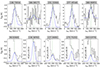 |
Fig. C.1. Top panel: 13CS. Bottom panel: 13C34S. Frequencies, in GHz, are labeled at the top of each sub-panel. Best-fit VLSR values (see Table C.1) are indicated by green-dashed vertical lines. The HC3N blending feature is indicated to the left of each 13CS transition. |
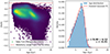 |
Fig. C.2. Metallicities and ages of the sample presented in Xiang & Rix (2022). Left panel: Metallicity-age relation color-coded by density with our derived metallicity range from sulfur isotopologue ratios. Right: Age distribution for the considered metallicity range indicating its mean value and 1σ uncertainty from a single Gaussian fit. |
Appendix D: Comparison among different methodologies
Results on the sSFRs
Given the different SED modeling approaches, that differ in terms of star formation histories and several other assumptions, here we provide a few comparison plots. Depending directly on the SED shape, we will obtain a sSFR (Conroy 2013). Then, each model assumes a certain mass-to-light ratio to derive the stellar mass and a specific SFH to derive the stellar ages, combining both results, mass and time, to obtain the SFR. Given the variation between GalaPy and CIGALE modeled SED shapes, as seen in Fig. 3, we expect dispersion in their resulting sSFRs, but a relative tendency to be a one-to-one relation. Such a tendency is seen in the bottom right panel of our Fig. D.1, whose values are listed in Table D.1, meaning that, at this level of comparison, both codes share similarities. From that same Figure it can be noted that GalaPy tends to produce larger SFRs and stellar masses, as also previously noted by Ronconi et al. (2024). The dust mass is mostly consistent between the GalaPy and CIGALE models within 1σ uncertainties for the less massive GMCs but systematically shifts toward the lower values of CIGALE compared to the higher values of GalaPy, as evidenced by the 1:1 red line in the bottom left panel of Fig. D.1. This trend becomes more pronounced in the more nuclear and massive regions, specifically GMCs 4–6 and also GMC 7.
In Fig. D.2, we compare the stellar population ages, burst ages, SF characteristic timescales, and ages weighted by light and mass, as provided by the different models utilized in this work. Specifically, CIGALE provides the main stellar population age, the late starburst age, the burst age, and the average age of the young and old stellar populations. From STARLIGHT, we include the averaged stellar ages weighted by light and by mass, which primarily correspond to the young and old stellar populations, respectively. Additionally, we present the stellar ages derived by GalaPy, along with the characteristic star-formation timescale, τ⋆, obtained from the same code.
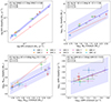 |
Fig. D.1. Comparison between the instantaneous SFR, the stellar mass (M★), the dust mass (Mdust), and sSFR derived from GalaPy (G; y-axes) and CIGALE (C; x-axes). GMCs are color-coded following the legend at the middle panel. All fits were performed on log-transformed data, except for the SFR, which was fitted using the linear scale. Linear regression was initially performed using the linregress function from the SciPy package (Gommers et al. 2025), followed by Bayesian inference through Markov chain Monte Carlo (MCMC) sampling implemented in the emcee package (Foreman-Mackey et al. 2013). |
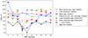 |
Fig. D.2. GMC stellar ages and burst estimations as traced by GalaPy, STARLIGHT, and CIGALE. SF peaks (SF characteristic timescale, τ⋆, from GalaPy in blue and last burst age from CIGALE in black) are also given for comparison. |
Appendix E: Testing the FIR bump accuracy
We have performed an SED fitting with both GalaPy and CIGALE considering a 9″ aperture diameter to include Herschel PACS data in the far infrared. This approach ensures that the infrared bump more accentuated in GalaPy than in CIGALE models (see Fig. 3 for a clear comparison) at around 100μm is properly fit without extrapolations. Additionally, it allows us to test whether our extrapolation was consistent with real observations, which cannot be verified at 3″ due to instrumental limitations. We found a similar dust temperature, which is a result driven by the FIR SED peak, in both cases, at 3 and 9″, as already pointed out in Sect. 5.1. Overall, the SED model used in GalaPy for GMC 5 correlates well with the one derived for the larger 9″ aperture centered at the same GMC.
In contrast, while CIGALE models underpredict the FIR bump in several GMCs compared to GalaPy, incorporating Herschel photometric points at 70, 100, and 160μm enables the code to fit all SED points accurately, regardless of whether an AGN component is assumed. The 9″ SED fitting using CIGALE is shown in the bottom middle panel of Figs. A.1 and A.2 for the cases without and with an AGN component, respectively. Interestingly, the SFRs differ by less than 5% between these models, reaffirming that the presence of an AGN is irrelevant from the SED perspective, as previously discussed inSect. 4.2.1.
Finally, the 3″ and 9″ SED models from GalaPy are shown in the right panel of Fig. E.1. The 3″ aperture SED corresponds to what was already presented in Fig. 3 for GMC 5.
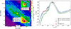 |
Fig. E.1. Testing the far infrared bump with Herschel PACS instruments. Left: Flux density of the S-PLUS R-filter band following the levels indicated in the colorbar. The two insets provide a closer look into the inner regions, where the CMZ is located. The upper inset shows the ten GMCs studied in this work, along with the ellipses where Lindblad resonances were detected by Iodice et al. (2014). The labeled apertures show how coarse (factor of 6–12 compared to the 3″ aperture used in this work) the angular resolution of Herschel SPIRE is from tracing our observations. The bottom inset performs a further 40% zooming on the nuclear regions, with Herschel PACS instrument apertures overlaid on the regions, and showing how GMCs 3 to 6 are partially or fully covered at 70, 100, and 160 μm observations beams. The contours show the L-band VLA observations (1.4 GHz) to indicate the maximum extent at which the rightmost point in our SEDs, namely, the largest wavelength, is available. Right: Visualization of Herschel PACS apertures and SED combined results. 3 and 9″ aperture SEDs obtained by GalaPy and centered at the GMC 5 position are in green and blue, respectively. We note that 6″ and 9″-aperture-extracted SED do not vary significantly (6″ SED is not shown) indicating that HST, VLT, and ALMA observations correspond to the central emission that does not increment with larger apertures. We consider only the 9″-aperture-extracted SED for comparison with the 3″ one as it better covers Herschel PACS observations at 70 and 100 μm bands, whose respective angular resolutions are of 5.6″ and 6.8″. Red points with an assumed 10% uncertainty correspond to the dataset used in Beck et al. (2022), their Table 4, to produce the SED of their Fig. 8, excluding GALEX observations as we have not used UV information for this work. |
All Tables
The extinction-related results obtained from SED modeling with CIGALE, including the AGN component.
Dust and SFH related results obtained from SED modeling with CIGALE, including AGN component.
Gas, star-formation (SF) related parameters and dust-related parameters for all SED results derived from GalaPy.
All Figures
|
Fig. 1. Work overview. From left to right and top to bottom: Labeled panels show: a) S-PLUS footprint scan over the southern hemisphere, where each light blue square represents a single S-PLUS observation (FoV of 1.4 × 1.4 deg2). b) Zoom-in on the S-PLUS field where NGC 253 is located, called field −s20s09, where an inset provides a closer view into the nuclear regions of this galaxy. Within the latter inset, there is another inset zooming in toward NGC 253’s CMZ, which is shown in the next panel. c) Here, we indicate the Hα (MUSE) emission as red contours and shaded areas, showing the strong stellar outflow observed at optical wavelengths. Complementing the latter, in the same panel, we show mainly in blue and white the integrated intensity of the CN 1–0 line at ∼113.4 GHz taken from ALCHEMI observations at 1 |
| In the text | |
|
Fig. 2. Integrated intensity maps of NGC 253’s CMZ showing its ten GMCs at the central frequencies of ALMA bands 3, 4, 6, and 7 (i.e., at 100, 144, 243, and 324 GHz). Data from ALMA band 5 are not shown as its central frequency of 187 GHz is strongly affected by telluric absorption from a water line at ∼183 GHz, as can be inferred from Fig. 1. The ALCHEMI 1 |
| In the text | |
|
Fig. 3. SED models obtained with the GalaPy software for the ten GMCs studied in this work, each of them covering a diameter of 3″ (∼50 pc; see Sect. 3.1). Points correspond to the photometric measurements obtained from the sample (Sects. 2 and 4.1), while solid lines correspond to the unattenuated stellar emission (green), molecular cloud component (MC, purple), stellar emission considering extinction (extinct, red), and diffuse dust (DD, yellow). Best-fitting modeling results from CIGALE, devoid of an AGN component, are overlaid as solid blue lines (see also Fig. A.1 for a detailed view). Detailed information about the CIGALE modeling is given in Appendix A. |
| In the text | |
|
Fig. 4. Stellar and dust masses of the analyzed GMCs derived by GalaPy (see Subsect. 4.1.1). Their different ranges are indicated in the central labels. |
| In the text | |
|
Fig. 5. STARLIGHT fits (shown by blue lines) are applied to the MUSE spectra (represented in black, with yellow lines indicating masked data) along with S-PLUS photometry fits (depicted with black and red circles, depending on whether they were used in the fit, with red points marking the masked data, and cyan points for the S-PLUS photometric data fitted by STARLIGHT). Vertical dashed lines indicate the position of the stellar features labeled in the top panels. |
| In the text | |
|
Fig. 6. STARLIGHT and GalaPy star-formation histories for the GMCs studied in this work. STARLIGHT discriminates between light and mass contributions to the total emission, contribution mainly coming from recent (blue) and old (red) stellar populations, respectively. GalaPy (black) generally provides ages between STARLIGHT’s light- and mass-weighted ages. For GMC 5, we have over-plotted the cumulative (in yellow) and normalized (in magenta) skewed Gaussian derived from the age-metallicity relation (see Appendix C). GMCs 3 to 6 also show the estimated ages from super star clusters derived by Butterworth et al. (2024) in vertical dashed blue lines surrounded by 1σ uncertainties as shaded areas; the remaining cumulative fraction (Cum. Frac.) to reach 100% of the emission at those ages, that is to say, the percentage of stellar formation that these radio observations account for, are denoted as r.l.f. and r.m.f. for remaining light and mass fractions, respectively. |
| In the text | |
|
Fig. 7. WHAN (left) and BPT (right) diagnostic diagrams (see Sect. 4.2.1) for the ten GMC studied using emission line ratios of the optical spectra from MUSE. We prefer the term “starburst+shocks” (SB+Shocks) over the commonly used “composite” given the findings highlighted in Sect. 4.2.1. |
| In the text | |
|
Fig. 8. Attenuation curves normalized at A(λ)/AV = 1 when λ = 5500 Å over wavelength in the rest frame, as derived by GalaPy SED fittings. The A(λ) value at 5500 Å is labeled in the legend of the left panel in linear scale and per GMC. This legend also indicates the color corresponding to each GMC in the solid lines. Curves based on RV values according to the methodology of Calzetti et al. (2000) are included for comparison (as dotted curves) in the left panel, following the colorbar. On the other hand, the dotted curves on the right panel show the attenuation curves from the models of Charlot & Fall (2000), which differentiate between young and old stellar populations, providing different exponential factors to the attenuation coming from birth clouds (BCs) and the ISM (ISM), related to these populations (see Sect. 4.2.2), which are labeled in the colorbar. |
| In the text | |
|
Fig. 9. Relation between absolute attenuation differences, |Δ AV|, obtained from the Balmer decrement, |
| In the text | |
|
Fig. 10. Star formation rate (SFR) obtained from Hα, SFRHα, following Eq. (5) versus the ones obtained from our SED fittings using GalaPy (red points; SFR in Table 5) and CIGALE (blue points; SFR10 Myr in Table 6), following the legend. The numbers correspond to the identification of the GMCs. Shaded areas indicate the 1σ dispersion for GalaPy (red) and CIGALE (SFRs averaged over 10 Myr in blue and over 100 Myr in gray) datapoints. The dashed black line shows the 1:1 expected correlation (Kennicutt 1998). The SFR obtained from the Hα emission line has been corrected by Balmer inferred attenuations |
| In the text | |
|
Fig. 11. SFR of the inner regions of NGC 253’s CMZ as accounted from the H40α RRL. The original ALCHEMI beam of 1 |
| In the text | |
|
Fig. 12. Star formation rate (SFR) of the inner regions of NGC 253’s CMZ. In the x-axis, the SFR is obtained from the H40α RRL (see Subsect. 4.3.2). In the y-axis, the SFR was obtained from the Ka EVLA band, applying the best-fitting relation from our linear regression, presented in Eq. (6). The resulting fit considering all data points (all) and per GMC (color-coded) are labeled along with the Pearson correlation coefficient, ⟨R⟩. All points include 10% uncertainties, with regression handling errors in both axes via Markov Chain Monte Carlo, as described in our Subsect. 4.2.3. |
| In the text | |
|
Fig. 13. SFR from our SED fitting using GalaPy versus fluxes from our retrieved (E)VLA continuum images, using apertures of 3″ in available GMCs (see Table 2). Best-fit linear regressions in the logarithmic scale are indicated in the top leftmost corners of each subplot, this best-fit is indicated with a dashed red line. The 1σ dispersion from the best fit to the different measurements is indicated in the bottom right corners of each subplot and also as shaded blue areas around the linear regression. (E)VLA band names are labeled with black background legends. GMCs are numbered and also color-coded following legend in Fig. D.1. We assume a conservative 10% flux uncertainty for (E)VLA observations. |
| In the text | |
|
Fig. 14. Same as in Fig. 13, but using IR SED fitting values, both from monochromatic fluxes (at 24, 60, and 100 μm) and from integrating the total infrared luminosity range (LIR; 8–1000 μm). GMCs are numbered and also color-coded following the legend in Fig. D.1. |
| In the text | |
|
Fig. A.1. Best-fit CIGALE SEDs without an AGN component of the ten GMCs studied here plus a 9″ aperture SED for the nuclear region, also devoid of an AGN component, in the bottom middle panel. Open blue circles are the observed fluxes while filled red points indicate modeled fluxes whose observed values may or may not be fitted, depending on their availability (see Table 2). The goodness of fit is estimated by the reduced χ2 shown at the top of each panel, along with the name and redshift of the GMC. In almost all cases, SEDs are well modeled, giving reasonable estimates of astrophysical properties. In Fig. A.2 we show our best-fits CIGALE models considering an AGN component. |
| In the text | |
|
Fig. A.2. Best-fit CIGALE+AGN SEDs of the ten GMCs studied here plus a 9″ aperture SED for the nuclear region, also considering an AGN component, in the bottom middle panel. Open blue circles are the observed fluxes while filled red points indicate modeled fluxes whose observed values may or may not be fitted, depending on their availability (see Table 2). The goodness of fit is estimated by the reduced χ2 shown at the top of each panel, along with the name and redshift of the GMC. In almost all cases, SEDs are well modeled, giving reasonable estimates of astrophysical properties. |
| In the text | |
|
Fig. C.1. Top panel: 13CS. Bottom panel: 13C34S. Frequencies, in GHz, are labeled at the top of each sub-panel. Best-fit VLSR values (see Table C.1) are indicated by green-dashed vertical lines. The HC3N blending feature is indicated to the left of each 13CS transition. |
| In the text | |
|
Fig. C.2. Metallicities and ages of the sample presented in Xiang & Rix (2022). Left panel: Metallicity-age relation color-coded by density with our derived metallicity range from sulfur isotopologue ratios. Right: Age distribution for the considered metallicity range indicating its mean value and 1σ uncertainty from a single Gaussian fit. |
| In the text | |
|
Fig. D.1. Comparison between the instantaneous SFR, the stellar mass (M★), the dust mass (Mdust), and sSFR derived from GalaPy (G; y-axes) and CIGALE (C; x-axes). GMCs are color-coded following the legend at the middle panel. All fits were performed on log-transformed data, except for the SFR, which was fitted using the linear scale. Linear regression was initially performed using the linregress function from the SciPy package (Gommers et al. 2025), followed by Bayesian inference through Markov chain Monte Carlo (MCMC) sampling implemented in the emcee package (Foreman-Mackey et al. 2013). |
| In the text | |
|
Fig. D.2. GMC stellar ages and burst estimations as traced by GalaPy, STARLIGHT, and CIGALE. SF peaks (SF characteristic timescale, τ⋆, from GalaPy in blue and last burst age from CIGALE in black) are also given for comparison. |
| In the text | |
|
Fig. E.1. Testing the far infrared bump with Herschel PACS instruments. Left: Flux density of the S-PLUS R-filter band following the levels indicated in the colorbar. The two insets provide a closer look into the inner regions, where the CMZ is located. The upper inset shows the ten GMCs studied in this work, along with the ellipses where Lindblad resonances were detected by Iodice et al. (2014). The labeled apertures show how coarse (factor of 6–12 compared to the 3″ aperture used in this work) the angular resolution of Herschel SPIRE is from tracing our observations. The bottom inset performs a further 40% zooming on the nuclear regions, with Herschel PACS instrument apertures overlaid on the regions, and showing how GMCs 3 to 6 are partially or fully covered at 70, 100, and 160 μm observations beams. The contours show the L-band VLA observations (1.4 GHz) to indicate the maximum extent at which the rightmost point in our SEDs, namely, the largest wavelength, is available. Right: Visualization of Herschel PACS apertures and SED combined results. 3 and 9″ aperture SEDs obtained by GalaPy and centered at the GMC 5 position are in green and blue, respectively. We note that 6″ and 9″-aperture-extracted SED do not vary significantly (6″ SED is not shown) indicating that HST, VLT, and ALMA observations correspond to the central emission that does not increment with larger apertures. We consider only the 9″-aperture-extracted SED for comparison with the 3″ one as it better covers Herschel PACS observations at 70 and 100 μm bands, whose respective angular resolutions are of 5.6″ and 6.8″. Red points with an assumed 10% uncertainty correspond to the dataset used in Beck et al. (2022), their Table 4, to produce the SED of their Fig. 8, excluding GALEX observations as we have not used UV information for this work. |
| In the text | |
Current usage metrics show cumulative count of Article Views (full-text article views including HTML views, PDF and ePub downloads, according to the available data) and Abstracts Views on Vision4Press platform.
Data correspond to usage on the plateform after 2015. The current usage metrics is available 48-96 hours after online publication and is updated daily on week days.
Initial download of the metrics may take a while.