| Issue |
A&A
Volume 697, May 2025
Euclid on Sky
|
|
|---|---|---|
| Article Number | A11 | |
| Number of page(s) | 45 | |
| Section | Extragalactic astronomy | |
| DOI | https://doi.org/10.1051/0004-6361/202450808 | |
| Published online | 30 April 2025 | |
Euclid: Early Release Observations – Overview of the Perseus cluster and analysis of its luminosity and stellar mass functions★
1
Université Paris-Saclay, Université Paris Cité, CEA, CNRS, AIM,
91191
Gif-sur-Yvette,
France
2
INAF-Osservatorio di Astrofisica e Scienza dello Spazio di Bologna,
Via Piero Gobetti 93/3,
40129
Bologna,
Italy
3
Aix-Marseille Université, CNRS, CNES, LAM,
Marseille,
France
4
INAF – Osservatorio Astronomico di Cagliari,
Via della Scienza 5,
09047
Selargius
(CA),
Italy
5
Universität Innsbruck, Institut für Astro- und Teilchenphysik,
Technikerstr. 25/8,
6020
Innsbruck,
Austria
6
Univ. Lille, CNRS, Centrale Lille,
UMR 9189 CRIStAL,
59000
Lille,
France
7
Université Paris-Saclay, CNRS, Institut d’astrophysique spatiale,
91405
Orsay,
France
8
Leibniz-Institut für Astrophysik (AIP),
An der Sternwarte 16,
14482
Potsdam,
Germany
9
Department of Physics, Université de Montréal,
2900 Edouard Montpetit Blvd, Montréal,
Québec
H3T 1J4,
Canada
10
Departamento de Física Teórica, Atómica y Óptica, Universidad de Valladolid,
47011
Valladolid,
Spain
11
Instituto de Astrofísica e Ciências do Espaço, Faculdade de Ciências, Universidade de Lisboa, Tapada da Ajuda,
1349-018
Lisboa,
Portugal
12
INAF – Osservatorio Astronomico d’Abruzzo, Via Maggini,
64100
Teramo,
Italy
13
Universitäts-Sternwarte München, Fakultät für Physik, Ludwig-Maximilians-Universität München,
Scheinerstrasse 1,
81679
München,
Germany
14
School of Physics and Astronomy, University of Nottingham,
University Park,
Nottingham
NG7 2RD,
UK
15
Centre de Recherche Astrophysique de Lyon, UMR5574, CNRS,
Université Claude Bernard Lyon 1, ENS de Lyon,
69230
Saint-Genis-Laval,
France
16
INAF-Osservatorio Astrofisico di Arcetri,
Largo E. Fermi 5,
50125
Firenze,
Italy
17
Université de Strasbourg, CNRS, Observatoire astronomique de Strasbourg,
UMR 7550,
67000
Strasbourg,
France
18
Kapteyn Astronomical Institute, University of Groningen,
PO Box 800,
9700
AV
Groningen,
The Netherlands
19
UK Astronomy Technology Centre, Royal Observatory,
Blackford Hill,
Edinburgh
EH9 3HJ,
UK
20
Department of Astronomy, University of Geneva,
ch. d’Ecogia 16,
1290
Versoix,
Switzerland
21
INAF – Osservatorio Astronomico di Capodimonte,
Via Moiariello 16,
80131
Napoli,
Italy
22
Institut universitaire de France (IUF),
1 rue Descartes,
75231
Paris CEDEX 05,
France
23
Laboratoire d’Astrophysique de Bordeaux, CNRS and Université de Bordeaux,
Allée Geoffroy St. Hilaire,
33165
Pessac,
France
24
NRC Herzberg,
5071 West Saanich Rd,
Victoria,
BC
V9E 2E7,
Canada
25
Max Planck Institute for Extraterrestrial Physics,
Giessenbachstr. 1,
85748
Garching,
Germany
26
European Space Agency/ESTEC,
Keplerlaan 1,
2201
AZ
Noordwijk,
The Netherlands
27
Max-Planck-Institut für Astronomie,
Königstuhl 17,
69117
Heidelberg,
Germany
28
Johns Hopkins University
3400 North Charles Street
Baltimore,
MD
21218,
USA
29
Sterrenkundig Observatorium, Universiteit Gent,
Krijgslaan 281 S9,
9000
Gent,
Belgium
30
INAF – Osservatorio Astronomico di Trieste,
Via G. B. Tiepolo 11,
34143
Trieste,
Italy
31
Jodrell Bank Centre for Astrophysics, Department of Physics and Astronomy, University of Manchester,
Oxford Road,
Manchester
M13 9PL,
UK
32
Institut d’Astrophysique de Paris, UMR 7095, CNRS, and Sorbonne Université,
98 bis boulevard Arago,
75014
Paris,
France
33
Universidad de La Laguna, Departamento de Astrofísica,
38206
La Laguna, Tenerife,
Spain
34
Instituto de Astrofísica de Canarias, Vía Láctea,
38205
La Laguna, Tenerife,
Spain
35
Aix-Marseille Université, CNRS/IN2P3, CPPM,
Marseille,
France
36
Institute of Physics, Laboratory of Astrophysics, Ecole Polytechnique Fédérale de Lausanne (EPFL), Observatoire de Sauverny,
1290
Versoix,
Switzerland
37
Université Paris Cité, CNRS, Astroparticule et Cosmologie,
75013
Paris,
France
38
Laboratoire de Physique de l’École Normale Supérieure, ENS, Université PSL, CNRS, Sorbonne Université,
75005
Paris,
France
39
STAR Institute, University of Liège, Quartier Agora,
Allée du six Août 19c,
4000
Liège,
Belgium
40
Space physics and astronomy research unit, University of Oulu,
Pentti Kaiteran katu 1,
90014
Oulu,
Finland
41
INAF-Osservatorio Astronomico di Roma,
Via Frascati 33,
00078
Monteporzio Catone,
Italy
42
Dipartimento di Fisica e Astronomia, Università di Firenze,
via G. Sansone 1,
50019
Sesto Fiorentino, Firenze,
Italy
43
University of Trento,
Via Sommarive 14,
38123
Trento,
Italy
44
Institute of Astronomy, University of Cambridge,
Madingley Road,
Cambridge
CB3 0HA,
UK
45
ESAC/ESA, Camino Bajo del Castillo, s/n., Urb. Villafranca del Castillo,
28692
Villanueva de la Cañada, Madrid,
Spain
46
School of Mathematics and Physics, University of Surrey, Guildford,
Surrey,
GU2 7XH,
UK
47
INAF-Osservatorio Astronomico di Brera,
Via Brera 28,
20122
Milano,
Italy
48
Dipartimento di Fisica e Astronomia, Università di Bologna,
Via Gobetti 93/2,
40129
Bologna,
Italy
49
INFN-Sezione di Bologna,
Viale Berti Pichat 6/2,
40127
Bologna,
Italy
50
INAF – Osservatorio Astronomico di Padova,
Via dell’Osservatorio 5,
35122
Padova,
Italy
51
IFPU, Institute for Fundamental Physics of the Universe,
via Beirut 2,
34151
Trieste,
Italy
52
INAF – Osservatorio Astrofisico di Torino,
Via Osservatorio 20,
10025
Pino Torinese
(TO),
Italy
53
Dipartimento di Fisica, Università di Genova,
Via Dodecaneso 33,
16146,
Genova,
Italy
54
INFN-Sezione di Genova,
Via Dodecaneso 33,
16146,
Genova,
Italy
55
Department of Physics “E. Pancini”, University Federico II,
Via Cinthia 6,
80126,
Napoli,
Italy
56
INFN section of Naples,
Via Cinthia 6,
80126
Napoli,
Italy
57
Instituto de Astrofísica e Ciências do Espaço, Universidade do Porto, CAUP, Rua das Estrelas,
4150-762
Porto,
Portugal
58
Faculdade de Ciências da Universidade do Porto, Rua do Campo de Alegre,
4150-007
Porto,
Portugal
59
Dipartimento di Fisica, Università degli Studi di Torino,
Via P. Giuria 1,
10125
Torino,
Italy
60
INFN-Sezione di Torino,
Via P. Giuria 1,
10125
Torino,
Italy
61
INAF-IASF Milano,
Via Alfonso Corti 12,
20133
Milano,
Italy
62
Centro de Investigaciones Energéticas, Medioambientales y Tecnológicas (CIEMAT),
Avenida Complutense 40,
28040
Madrid,
Spain
63
Port d’Informació Científica, Campus UAB, C. Albareda s/n,
08193
Bellaterra (Barcelona),
Spain
64
Institute for Theoretical Particle Physics and Cosmology (TTK), RWTH Aachen University,
52056
Aachen,
Germany
65
Institute of Space Sciences (ICE, CSIC), Campus UAB, Carrer de Can Magrans, s/n,
08193
Barcelona,
Spain
66
Institut d’Estudis Espacials de Catalunya (IEEC), Edifici RDIT, Campus UPC,
08860
Castelldefels, Barcelona,
Spain
67
Dipartimento di Fisica e Astronomia “Augusto Righi” – Alma Mater Studiorum Università di Bologna,
Viale Berti Pichat 6/2,
40127
Bologna,
Italy
68
Institute for Astronomy, University of Edinburgh, Royal Observatory,
Blackford Hill,
Edinburgh
EH9 3HJ,
UK
69
European Space Agency/ESRIN,
Largo Galileo Galilei 1,
00044
Frascati, Roma,
Italy
70
Université Claude Bernard Lyon 1, CNRS/IN2P3, IP2I Lyon,
UMR 5822,
Villeurbanne
69100,
France
71
UCB Lyon 1, CNRS/IN2P3, IUF, IP2I Lyon,
4 rue Enrico Fermi,
69622
Villeurbanne,
France
72
Mullard Space Science Laboratory, University College London,
Holmbury St Mary, Dorking,
Surrey
RH5 6NT,
UK
73
Departamento de Física, Faculdade de Ciências, Universidade de Lisboa,
Edifício C8, Campo Grande,
1749-016
Lisboa,
Portugal
74
Instituto de Astrofísica e Ciências do Espaço, Faculdade de Ciências, Universidade de Lisboa, Campo Grande,
1749-016
Lisboa,
Portugal
75
INAF – Istituto di Astrofisica e Planetologia Spaziali,
via del Fosso del Cavaliere, 100,
00100
Roma,
Italy
76
INFN-Padova,
Via Marzolo 8,
35131
Padova,
Italy
77
School of Physics, HH Wills Physics Laboratory, University of Bristol,
Tyndall Avenue,
Bristol
BS8 1TL,
UK
78
Istituto Nazionale di Fisica Nucleare, Sezione di Bologna,
Via Irnerio 46,
40126
Bologna,
Italy
79
FRACTAL S.L.N.E.,
calle Tulipán 2, Portal 13 1A,
28231,
Las Rozas de Madrid,
Spain
80
Dipartimento di Fisica “Aldo Pontremoli”, Università degli Studi di Milano,
Via Celoria 16,
20133
Milano,
Italy
81
Institute of Theoretical Astrophysics, University of Oslo,
PO Box 1029 Blindern,
0315
Oslo,
Norway
82
Leiden Observatory, Leiden University,
Einsteinweg 55,
2333
CC
Leiden,
The Netherlands
83
Jet Propulsion Laboratory, California Institute of Technology,
4800 Oak Grove Drive,
Pasadena,
CA
91109,
USA
84
Department of Physics, Lancaster University,
Lancaster
LA1 4YB,
UK
85
Felix Hormuth Engineering,
Goethestr. 17,
69181
Leimen,
Germany
86
Technical University of Denmark,
Elektrovej 327,
2800
Kgs. Lyngby,
Denmark
87
Cosmic Dawn Center (DAWN),
Denmark
88
NASA Goddard Space Flight Center,
Greenbelt,
MD
20771,
USA
89
Department of Physics and Helsinki Institute of Physics,
Gustaf Hällströmin katu 2,
00014
University of Helsinki,
Finland
90
Université de Genève, Département de Physique Théorique and Centre for Astroparticle Physics,
24 quai Ernest-Ansermet,
CH-1211
Genève 4,
Switzerland
91
Department of Physics,
PO Box 64,
00014
University of Helsinki,
Finland
92
Helsinki Institute of Physics,
Gustaf Hällströmin katu 2,
University of Helsinki, Helsinki,
Finland
93
Department of Physics and Astronomy, University College London,
Gower Street,
London
WC1E 6BT,
UK
94
NOVA optical infrared instrumentation group at ASTRON,
Oude Hoogeveensedijk 4,
7991PD
Dwingeloo,
The Netherlands
95
INFN-Sezione di Milano,
Via Celoria 16,
20133
Milano,
Italy
96
Universität Bonn, Argelander-Institut für Astronomie,
Auf dem Hügel 71,
53121
Bonn,
Germany
97
Dipartimento di Fisica e Astronomia “Augusto Righi” – Alma Mater Studiorum Università di Bologna,
via Piero Gobetti 93/2,
40129
Bologna,
Italy
98
Department of Physics, Centre for Extragalactic Astronomy, Durham University,
South Road,
Durham
DH1 3LE,
UK
99
Department of Physics, Institute for Computational Cosmology, Durham University,
South Road,
Durham
DH1 3LE,
UK
100
Université Côte d’Azur, Observatoire de la Côte d’Azur, CNRS, Laboratoire Lagrange,
Bd de l’Observatoire, CS 34229,
06304
Nice cedex 4,
France
101
University of Applied Sciences and Arts of Northwestern Switzerland, School of Engineering,
5210
Windisch,
Switzerland
102
Institut d’Astrophysique de Paris,
98bis Boulevard Arago,
75014
Paris,
France
103
Aurora Technology for European Space Agency (ESA), Camino bajo del Castillo, s/n, Urbanizacion Villafranca del Castillo, Villanueva de la Cañada,
28692
Madrid,
Spain
104
Institut de Física d’Altes Energies (IFAE), The Barcelona Institute of Science and Technology, Campus UAB,
08193
Bellaterra (Barcelona),
Spain
105
Department of Physics and Astronomy, University of Aarhus,
Ny Munkegade 120,
8000
Aarhus C,
Denmark
106
Waterloo Centre for Astrophysics, University of Waterloo, Waterloo,
Ontario
N2L 3G1,
Canada
107
Department of Physics and Astronomy, University of Waterloo, Waterloo,
Ontario
N2L 3G1,
Canada
108
Perimeter Institute for Theoretical Physics, Waterloo,
Ontario
N2L 2Y5,
Canada
109
Space Science Data Center, Italian Space Agency, via del Politecnico snc,
00133
Roma,
Italy
110
Centre National d’Etudes Spatiales – Centre spatial de Toulouse,
18 avenue Edouard Belin,
31401
Toulouse Cedex 9,
France
111
Institute of Space Science,
Str. Atomistilor, nr. 409 Măgurele,
Ilfov,
077125,
Romania
112
Dipartimento di Fisica e Astronomia “G. Galilei”, Università di Padova,
Via Marzolo 8,
35131
Padova,
Italy
113
Departamento de Física, FCFM, Universidad de Chile, Blanco Encalada
2008,
Santiago,
Chile
114
Satlantis, University Science Park,
Sede Bld
48940,
Leioa-Bilbao,
Spain
115
Centre for Electronic Imaging, Open University,
Walton Hall,
Milton Keynes
MK7 6AA,
UK
116
Infrared Processing and Analysis Center, California Institute of Technology,
Pasadena,
CA
91125,
USA
117
Universidad Politécnica de Cartagena, Departamento de Electrónica y Tecnología de Computadoras,
Plaza del Hospital 1,
30202
Cartagena,
Spain
118
Institut de Recherche en Astrophysique et Planétologie (IRAP), Université de Toulouse, CNRS, UPS, CNES,
14 Av. Edouard Belin,
31400
Toulouse,
France
119
INFN-Bologna,
Via Irnerio 46,
40126
Bologna,
Italy
120
INAF, Istituto di Radioastronomia,
Via Piero Gobetti 101,
40129
Bologna,
Italy
121
ICL, Junia, Université Catholique de Lille, LITL,
59000
Lille,
France
122
Department of Physics and Astronomy, University of British Columbia,
Vancouver,
BC
V6T 1Z1,
Canada
★★ Corresponding author; jc.cuillandre@cea.fr
Received:
21
May
2024
Accepted:
13
March
2025
The Euclid Early Release Observations (ERO) programme targeted the Perseus cluster of galaxies, gathering deep data in the central region of the cluster over 0.7 deg2, including the cluster core up to 0.25 r200. The dataset reaches a point-source depth of IE = 28.0 (YE, JE, HE = 25.3), AB magnitudes at 5 σ with a 0′′.16 (0′′.48) full width at half maximum (FWHM), and a surface brightness limit of 30.1 (29.2) mag arcsec−2 for radially integrated galaxy profiles. The exceptional depth and spatial resolution of this wide-field multi-band data enable simultaneous detection and characterisation of both bright galaxies and low surface brightness ones, along with their globular cluster systems, from the optical to the near-infrared (NIR). Cluster membership was determined using several methods in order to maximise the completeness and minimise the contamination of foreground and background sources. We adopted a catalogue of 1100 dwarf galaxies, detailed in the corresponding ERO paper, that includes their photometric and structural properties. We identified all other sources in the Euclid images and obtained accurate photometric measurements using AutoProf or AstroPhot for 137 bright cluster galaxies and SourceExtractor for half a million compact sources. This study advances beyond previous analyses of the cluster and enables a range of scientific investigations, which are summarised here. We derived the luminosity and stellar mass functions (LF and SMF) of the Perseus cluster in the Euclid IE band thanks to supplementary u, g, r, i, z, and Hα data from the Canada-France-Hawai’i Telescope (CFHT). Our LF and SMF are the deepest recorded for the Perseus cluster, highlighting the groundbreaking capabilities of the Euclid telescope. We fit the LF and SMF with a Schechter plus Gaussian model. The LF features a dip at M(IE) ≃ −19 and a faint-end slope of αS ≃ −1.2 to −1.3. The SMF displays a low-mass-end slope of αS ≃ −1.2 to −1.35. These observed slopes are flatter than those predicted for dark matter halos in cosmological simulations, offering significant insights for models of galaxy formation and evolution.
Key words: galaxies: fundamental parameters / galaxies: clusters: individual: Perseus / galaxies: luminosity function, mass function
© The Authors 2025
 Open Access article, published by EDP Sciences, under the terms of the Creative Commons Attribution License (https://creativecommons.org/licenses/by/4.0), which permits unrestricted use, distribution, and reproduction in any medium, provided the original work is properly cited.
This article is published in open access under the Subscribe to Open model. Subscribe to A&A to support open access publication.
1 Introduction
The luminosity function (LF) and stellar mass function (SMF) have often been used in the literature to constrain cosmological simulations and semi-analytic models of galaxy evolution (e.g. Kauffmann et al. 1993; Kauffmann & Haehnelt 2000; Cole et al. 2000; Benson et al. 2003; Schaye et al. 2015; Pillepich et al. 2018). The number of objects detected in blind observations in given intervals of luminosity or mass can be easily compared to those predicted by simulations. When measured in the visible and NIR bands, the LF and the SMF trace the statistical weight of galaxies of different luminosities and stellar masses in relation to the total stellar emission of the Universe. Moreover, they can be measured in different intervals of redshift to study the evolution of galaxies with time (e.g. Efstathiou et al. 1988; Loveday et al. 1992; Lilly et al. 1995; Cole et al. 2001; Blanton et al. 2003; Bell et al. 2003; Faber et al. 2007; Pozzetti et al. 2010).
Comparison of observed LFs in the visible and NIR bands with the predictions of simulations has been crucial for understanding the importance of feedback in shaping galaxy evolution. The observed flat slope of the distribution compared to the steep rise at the faint end predicted by the first generation of cosmological simulations (the ‘missing satellite problem’) has been solved by including the contribution of feedback from supernovae. In low-mass systems, feedback is able to sweep away a considerable fraction of the cold interstellar medium (ISM) loosely bound to shallow gravitational potential wells, thus significantly reducing the star-formation activity in the disc. Feedback from an active galactic nucleus (AGN) has also been claimed to explain the observed abrupt decrease of luminous and massive galaxies at the bright end of the LF and SMF (e.g. White & Frenk 1991; Kauffmann et al. 1993; Somerville & Primack 1999; Benson et al. 2003; Somerville & Davé 2015), and in general the feedback processes and the interplay with the environment give rise to the different shape of the SMF compared to the halo mass function (Dekel & Birnboim 2006).
The LF and SMF are powerful statistical tools for characterising the properties of galaxies in different environments, from rich clusters to groups, filaments, and voids. Several studies seem to indicate that the properties of the LFs of galaxies in high-density regions are different than those derived in the field, where the slope at the faint end is generally flatter and the characteristic luminosity is lower than in rich clusters (Sandage et al. 1985; Balogh et al. 2001; De Propris et al. 2003; Lin et al. 2004; Hansen et al. 2005; Popesso et al. 2005; Boselli & Gavazzi 2006; Ferrarese et al. 2016). This systematic difference in the statistical distribution of galaxies has been explained as being related to the different evolutionary paths that they undergo in rich environments, where they suffer a large variety of perturbations (e.g Boselli & Gavazzi 2006, 2014; Boselli et al. 2022b). The brightest galaxies (centrals) are formed by multiple merging events in the most massive halos (Ostriker & Hausman 1977; De Propris et al. 2003; De Lucia & Blaizot 2007; Cappellari et al. 2011; Boselli et al. 2014), while dwarf systems can be formed in rich environments by galaxy harassment (Moore et al. 1998; Mastropietro et al. 2005b; Popesso et al. 2006; Barkhouse et al. 2007; de Filippis et al. 2011) or by the simple fading of the star-formation activity of galaxies undergoing a ram-pressure-stripping event (e.g. Boselli et al. 2008b,a; Boselli & Gavazzi 2014). The shape of the LF also changes as a function of wavelength, with redder galaxies being dominant in high-density regions and star-forming galaxies being dominant in the field (e.g. Blanton et al. 2005a), as expected for the well-known morphological segregation effect (e.g. Dressler 1980b; Whitmore et al. 1993; Dressler et al. 1997).
There are, however, several unclear questions that still need to be answered. The first of them concerns the contribution of low surface brightness (LSB) galaxies to the observed LF, particularly at the faint end where these systems can be dominant. Using a complete set of data extracted from the Sloan Digital Sky Survey (SDSS), Blanton et al. (2005a) showed that the faint end slope of the LF measured in the visible bands and parameterised with a Schechter (1976) function can drastically change from α ≃ −1 to α ≃ −1.5 (where α is the slope of the power-law distribution) when LSB galaxies are correctly accounted for. This steeper slope is still far from the one predicted for the dark matter halo mass function by cosmological simulations (α ≃ −2, e.g. Somerville & Davé 2015). It is rather similar to the one often observed in rich clusters where the LFs are measured using deep and very sensitive imaging data gathered using wide-field cameras coupled with 4–8 m class telescopes (e.g. Sandage et al. 1985; Popesso et al. 2006; Ferrarese et al. 2016). Presently, studies of the faint end of the LF and SMF can only be conducted on nearby clusters with deep imaging data able to detect LSB systems (e.g. van Dokkum et al. 2015b; Koda et al. 2015; Mihos et al. 2015; Venhola et al. 2017; van der Burg et al. 2017; Lim et al. 2020; Zöller et al. 2024) and in field and group environments Marleau et al. 2021). Further study of systems of varying halo mass should allow any possible dependence of the LF on the mass of the host dark matter halo to be traced and at the same time minimise the impact of sampling variance on our results.
The Euclid space mission (Euclid Collaboration: Mellier et al. 2025) has been designed to map with extraordinary sensitivity and image quality most of the extragalactic sky, Euclid Wide Survey (EWS), 14 000 deg2, in the visible and NIR wavelength range. In particular, the visible instrument (VIS) (Euclid Collaboration: Cropper et al. 2025) and the Near-Infrared Spectrometer and Photometer (NISP) (Euclid Collaboration: Jahnke et al. 2025) instruments are the first wide-field cameras sensitive to surface brightness levels of 29.8 and 28.4 mag arcsec−2 (Euclid Collaboration: Scaramella et al. 2022) in the visible and NIR bands, respectively, which are values never achieved before over such a wide area. The EWS will provide a unique set of photometric data to explore the LSB Universe and thus quantify, through solid statistical arguments, the contribution of LSB and ultra diffuse galaxies (UDGs), and dwarf systems in general, at the faint end of the LF. The four Euclid photometric bands used during the observations (IE, YE, JE, and HE) are sensitive to the bulk of the stellar emission and are thus optimal to infer the SMF with extreme accuracy. Covering a wide fraction of the sky, the EWS will be perfectly suited to deriving these statistical functions for galaxies in different environments, from rich clusters to voids and at different redshifts, thus providing a unique reference for comparison with the predictions of cosmological simulations on the mass assembly process in the Universe. The improvement with respect to SDSS will be substantial, while the synergy with the Ultraviolet Near Infrared Optical Northern Survey (UNIONS) in the northern hemisphere and Legacy Survey of Space and Time (LSST) in the south will be extremely useful for deriving photometric redshifts and physical properties of galaxies, hence enabling the study of the wavelength dependence of these statistical functions, which is fundamental for reconstructing the stellar evolution across time (Guy et al. 2022).
This paper presents the results obtained by the analysis of the data gathered during the Euclid Early Release Observations (ERO, Euclid Early Release Observations 2024) programme for the Perseus cluster of galaxies. This unique dataset is used to derive the LF and SMF of galaxies located within R ≃ 0.25 r200 of the cluster centre. Here, r200 is the radius within which the cluster density is 200 times the Universe’s critical density, a proxy for the virial radius. Being a nearby rich cluster of galaxies dominated by LSB early-type objects, Perseus is an excellent target for testing the unique capabilities of the telescope in the study of the LSB Universe. Located at a relatively low Galactic latitude (b ~ −13°), Perseus is also an optimal target to quantify the possible contamination of Galactic cirrus emission in these bands, providing us with a unique reference for all future Euclid extragalactic studies.
The comprehensive range of science cases explored by the ERO Perseus science team using this dataset is detailed in Appendix A. Each scientific programme demands high-quality data that preserve both resolution and photometric integrity for various astronomical objects, from compact sources such as stars, globular clusters, and field galaxies, to extended sources including large galaxies. Details of the specific efforts undertaken to process the ERO dataset are documented in Cuillandre et al. (2025), while this report focuses solely on the performance achieved for the Perseus field.
Accompanying this report on the LF and SMF of the Perseus cluster are two papers focusing on how these data have transformed our understanding of intra-cluster light (ICL) and intracluster globular clusters (ICGCs) and cluster dwarf galaxies (Kluge et al. 2025; Marleau et al. 2025).
This paper is structured as follows. We describe in Sect. 2 the main properties of the Perseus cluster. In Sect. 3, we detail the data used in the analysis. In Sect. 4, we present the multi-wavelength catalogues, and in Sect. 5, we show the methodology used to identify all cluster members. The LF and the SMF are derived in Sects. 6 and 7. The results are discussed in Sect. 8, and the conclusions are given in Sect. 9. In the following analysis, we used Galfit (Peng et al. 2010), AutoProf, and AstroPhot (Stone et al. 2021, 2023) to derive the structural parameters for galaxies identified as members of the Perseus cluster. We also used SourceExtractor to derive the multi-wavelength photometry for all the sources in the field. We adopted a standard flat ΛCDM cosmology with Ωm = 0.319 and H0 = 67 km s−1 Mpc−1 (Planck Collaboration VI 2020), and all magnitudes are given using the AB magnitude system.
2 The Perseus cluster
The Perseus cluster (Abell 426) is one of the most intensively studied high-density regions in the nearby Universe. Located at only 72 Mpc (Vc = 5258 km s−1, σc = 1040 km s−1; Aguerri et al. 2020) at the edge of the Taurus void (Batuski & Burns 1985), it belongs to the Perseus-Pisces supercluster, a large-scale structure in the southern sky extending more than 50 Mpc in the direction perpendicular to the line of sight (Chincarini et al. 1983; Wegner et al. 1993). Perseus is classified as a Bautz–Morgan type II-III cluster of richness class 2 (Bautz & Morgan 1970; Struble & Rood 1999), and hosts one of the most spectacular known core-cooling flows tightly connected with the central type-D giant elliptical galaxy NGC 1275 and its AGN activity (Conselice et al. 2001; Fabian et al. 2003b; Salomé et al. 2006). Perseus is also the brightest known X-ray cluster of galaxies (Edge et al. 1990), the target of several X-ray observations given its peculiar structure, with large-scale motions in the intragalactic medium (IGM) and complex metal enrichment history (e.g. Churazov et al. 2003; Sanders & Fabian 2007; Simionescu et al. 2012, 2019; Werner et al. 2013; Boyarsky et al. 2014; Aharonian et al. 2017; Lau et al. 2017; Sanders et al. 2020). X-ray observations also indicate that the cluster might not be fully relaxed (Ulmer et al. 1992; Churazov et al. 2003; Ichinohe et al. 2019). Additional peculiarities have been observed in the radio domain, with the presence of a mini-halo and cavities associated with radio-mode feedback from NGC 1275 (e.g. Soboleva et al. 1983; Boehringer et al. 1993; Gendron-Marsolais et al. 2017, 2020).
The cluster has been the target of several spectroscopic surveys aimed at identifying its galaxy members, including dwarf LSB systems (e.g. Chincarini & Rood 1971; Brunzendorf & Meusinger 1999; Penny & Conselice 2008; Wittmann et al. 2017, 2019; Aguerri et al. 2020; Meusinger et al. 2020). The spectroscopic data have also been used to derive the mean properties of the cluster, such as its radius and mass (r200 = 2.2 Mpc and M200 = 1.2 × 10¹⁵ M⊙, Aguerri et al. 2020). These values can be compared to the estimates of r200 = 1.79 Mpc and M200 = 6.65 × 10¹⁴ M⊙ derived from X-ray observations by Simionescu et al. (2012). The cluster population is dominated by earlytype systems with few spiral galaxies (Kent & Sargent 1983; Andreon 1994; Giovanelli et al. 1986), but it hosts a few star-forming galaxies with radio continuum morphologies witnessing an ongoing transformation (Roberts et al. 2022b, George et al., in prep.). The region analysed in this work covers 0.7 deg2 on the sky (1 Mpc2 at the Perseus distance), located within the inner ≃0.25 r200, where the density of galaxies is very high (around 3000 galaxies deg−2 at the distance of the cluster). Consistently with the other papers based on ERO data on the cluster, we assume a distance of 72 Mpc (m − M = 34.287, z = 0.0167).
3 Observations
The core of our dataset are the new deep Euclid observations of the Perseus cluster in the very broad filter IE (equivalent to r + i + z) in the optical from the VIS instrument (Cropper et al. 2016; Euclid Collaboration: Cropper et al. 2025) and the three broad filters YE, JE, and HE in the NIR from the NISP instrument (Maciaszek et al. 2016; Euclid Collaboration: Jahnke et al. 2025), combined in the image in Fig. 1.
To fully harness the scientific potential of the Euclid data, integrating complementary optical broad-band photometry is essential. This section briefly reviews the observations obtained with Euclid and their performance, alongside deep complementary MegaCam data acquired at the CFHT prior to the Euclid launch.
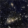 |
Fig. 1 Colour image of the Perseus cluster released worldwide by the ESA in November 2023. It was created by combining VIS and NISP Euclid images using the IE band in the blue, YE in the green, and HE in the red. The FoV of this image is 0.5 deg2, with the x- and y-axes aligned with the Euclid camera native pixel geometry (see Fig. 13 for an equatorial projection). The three brightest galaxies are NGC 1265 (top of the image), NGC 1272, and NGC 1275 (bottom, from right to left). Credit: ESA/Euclid/Euclid Consortium/NASA, image processing by J.-C. Cuillandre (CEA Paris-Saclay), G. Anselmi. |
3.1 Euclid VIS and NISP dataset
The Perseus cluster data were collected during the Euclid performance-verification phase in September 2023 (Cuillandre et al. 2025). All Euclid science observations adhere to a predetermined reference observing sequence (ROS, Euclid Collaboration: Scaramella et al. 2022), which consists of four dithered exposures lasting 566 s each in the IE filter, and four dithered exposures of 87.2 s each in the YE, JE, and HE filters. Their passbands are shown in Fig. 2 (Euclid Collaboration: Schirmer et al. 2022; Cropper et al. 2016; Euclid Collaboration: Scaramella et al. 2022).
Four ROSs were obtained in total on the Perseus cluster, two ROSs on 9 September, with a 3′ offset between the two ROSs, along the x, y common axis of both instruments. Due to an inversion of the dither axis, this set was duplicated on 16 September to mitigate signal-to-noise ratio (S/N) ratio variations across the detector mosaic gaps. In total, with these four ROSs, the integration time over the common field of view (FoV) of 0.7 deg2 between the two instruments is 7456.0 s in the IE filter and 1392.2 s in the YE, JE, and HE filters (see Table 1). This combination achieves a depth that is 0.75 mag deeper than the EWS for the compact sources, which relies on a single ROS (Euclid Collaboration: Scaramella et al. 2022). The data are of exceptional quality, benefiting from being gathered in a nominal spacecraft configuration.
The ERO data are meticulously detrended, calibrated, resampled, and stacked, as detailed in Cuillandre et al. (2025). The relative internal photometric calibration accuracy is evaluated at 5% – this represents the internal scatter for stars matched with Gaia-DR3 (Gaia Collaboration 2023) – while the absolute photometric calibration (zero points) achieves precision at the percent level. Astrometric precision using Gaia-DR3 as a reference reaches 8 mas for VIS and 15 mas for NISP, both representing less than a tenth of a pixel for each instrument across the entire FoV.
The ERO pipeline (Cuillandre et al. 2025) produces two distinct types of stacks for each Euclid band: an LSB stack designed to preserve all extended emission; and a stack optimised for compact sources science, which suppresses all diffuse emission beyond approximately 6″. This latter stack is referred to as the ‘compact-sources stack’, and the comparison with the LSB stack is illustrated in Fig. 3.
The pixel sizes for the VIS and NISP data are ![$\[0^{\prime \prime}_\cdot1\]$](/articles/aa/full_html/2025/05/aa50808-24/aa50808-24-eq3.png) and
and ![$\[0^{\prime \prime}_\cdot3\]$](/articles/aa/full_html/2025/05/aa50808-24/aa50808-24-eq4.png) , respectively, while the FWHM in the IE, YE, JE, and HE science stacks measures
, respectively, while the FWHM in the IE, YE, JE, and HE science stacks measures ![$\[0^{\prime \prime}_\cdot16, ~0^{\prime \prime}_\cdot48,~0^{\prime \prime}_\cdot49,\]$](/articles/aa/full_html/2025/05/aa50808-24/aa50808-24-eq5.png) , and
, and ![$\[0^{\prime \prime}_\cdot50\]$](/articles/aa/full_html/2025/05/aa50808-24/aa50808-24-eq6.png) , respectively. At the distance of the Perseus cluster, these values correspond to approximately 56 pc for VIS and 171 pc for NISP.
, respectively. At the distance of the Perseus cluster, these values correspond to approximately 56 pc for VIS and 171 pc for NISP.
Figure 1 presents a red-green-blue (RGB) colour image of the Perseus cluster, where extended diffuse emission is easily seen. The image background of each stack is dominated by zodiacal light (Euclid Collaboration: Scaramella et al. 2022), measured here at 22.3 mag arcsec−2 in IE, and 22.1, 22.3, and 22.5 mag arcsec−2 in YE, JE, and HE, respectively.
Section 9 of Cuillandre et al. (2025) reports that the sensitivity to LSB features of both instruments is exceptional thanks to Euclid’s unique optical design, and based on a depth metric assuming the absence of contaminants in the sky background, such as high stellar density or Galactic cirrus. Due to the presence of cirrus in the Perseus field (see Fig. 4), the limiting surface brightness is slightly degraded and the values are in Table 1.
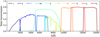 |
Fig. 2 Transmission of the Euclid and CFHT filters used in the present work. |
Properties of the Euclid dataset.
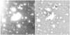 |
Fig. 3 Left: ERO pipeline LSB stack preserving all scales across the image. The pipeline is optimised for the photometry of extended objects such as these Perseus cluster galaxies. Right: ERO pipeline for compact-sources removing most of the LSB signal. The stack with internal background subtraction suppresses much of the signal from the large galaxies. The field size is 3′ by 3′. |
Properties of the CFHT-MegaCam dataset.
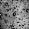 |
Fig. 4 Galactic cirrus contamination in the Perseus field. This illustration, particularly around UGC 2621 (located at the centre of the image), demonstrates the non-uniformity of the sky background in the IE filter. Here, the cirrus shines at surface brightness levels from 26.3 mag arcsec−2 (maximum) to 27.5 mag arcsec−2 (median), affecting the LSB detection performance. This contamination limits our ability to detect other extended emission, such as the outskirts of diffuse stellar halos. The FoV here is 5′ by 5′. |
3.2 CFHT-MegaCam dataset
In the context of the Euclid Surveys (Euclid Collaboration: Scaramella et al. 2022), complementary ground-based optical data are crucial for enhancing the Euclid dataset, particularly for deriving colours and computing photometric redshifts and physical properties of galaxies. Observations were conducted using MegaCam at the CFHT atop Maunakea, employing the u, g, r, i, and z filters, along with the Hα ‘off’ filter (CFHT ID 9604). This filter is centred on λc = 6719 Å with a width of Δλ = 109 Å, corresponding to a heliocentric velocity range of 4660 ≲ vhel/km s−1 ≲ 9600, making it well-suited to cover the velocity range of the Perseus cluster. An example of the Hα+[N II] stellar-continuum-subtracted image of the galaxy NGC 1275 is shown in Fig. 5, and compared to the IE image.
The observations took place during January and February 2021, November 2021, and September 2022, under dark skies and photometric conditions at an airmass of 1.3. Table 2 details the main properties of this dataset.
A very large dithering approach was employed for these observations, moving objects by up to 10′ along both camera axes. This scale surpasses the size of all astronomical objects in the field, including the large elliptical galaxies that necessitated this dithering strategy. Such extensive dithering facilitates a clean median model of the background, although it results in a loss of FoV in the final stacked images. Only the central region, where the S/N is relatively uniform, is retained.
The native camera FoV is 1.1 deg2, with a pixel resolution of 0.187 arcsec pixel−1. The final MegaCam stacks cover 1.2 deg2 and overlap with 95% of the Euclid observation (Fig. 6).
All images were detrended and calibrated using the Elixir pipeline (Magnier & Cuillandre 2004), and further processed with the Elixir-LSB pipeline, specifically designed for the Next Generation Virgo Survey (NGVS, Ferrarese et al. 2012), to detect extended LSB features. This pipeline was also applied to the narrow-band imaging for the Virgo Environmental Survey Tracing Ionised Gas Emission (VESTIGE, Boselli et al. 2018). Thanks to MegaCam’s well-calibrated and stable performance, no significant challenges were encountered in preparing this dataset, which was captured under excellent sky conditions.
Exceptional image quality was achieved using the Hα filter (FWHM ![$\[0^{\prime \prime}_\cdot49\]$](/articles/aa/full_html/2025/05/aa50808-24/aa50808-24-eq7.png) ), comparable to the Euclid NIR bands, and in a subset of r-band images that matched the FWHM criteria. The r-band image was employed to subtract a stellar continuum, producing a Hα+[N II] line emission image used in this study to identify signs of star formation and assess the membership of some galaxies in the Perseus cluster.
), comparable to the Euclid NIR bands, and in a subset of r-band images that matched the FWHM criteria. The r-band image was employed to subtract a stellar continuum, producing a Hα+[N II] line emission image used in this study to identify signs of star formation and assess the membership of some galaxies in the Perseus cluster.
In Fig. 7 we compare the depths of Euclid and CFHT data, to show that they match well, enhancing the quality of the multiband catalogue described in the following section.
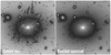 |
Fig. 5 Left: Image of Hα+[N II] emission from the galaxy NGC 1275 by CFHT. The filamentary structures show the cooling flow gas (e.g. Conselice et al. 2001). Right: Euclid IE image. The FoV per panel is 4′ by 4′. |
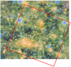 |
Fig. 6 Euclid Perseus area, marked in red and covering 0.7 deg2, shown against the broader coverage of the CFHT-MegaCam observations, which extend over 1.2 deg2. North is up, east is left. This high-contrast colour image is a composite RGB picture created from the MegaCam r, g, and u bands. The three brightest galaxies (NGC 1265, NGC 1272, and NGC 1275) can be spotted as large yellow blobs within the red footprint in the upper side and lower left corner of the Euclid FoV, with coordinates given in Fig. 24. The Galactic cirrus, which peaks in brightness in the g band, highlights the extent of contamination in this area, with an average E(B − V) of 0.156. While significantly fainter in the r band, the Galactic cirrus still impacts the VIS IE band, thereby limiting the low-surface brightness performance across the Euclid FoV. |
4 Compact sources multi-band photometric catalogue
The general effort for ERO processing and calibration (Cuillandre et al. 2025) was focused on providing all science teams with astrometrically and photometrically calibrated image stacks across all four Euclid bands, accompanied by comprehensive catalogues produced using the tool SourceExtractor (Bertin & Arnouts 1996). These versatile, science-ready catalogues are tailored exclusively for compact sources, utilising only the compact-sources stack while excluding the diffuse-emission stacks designed for tools such as AutoProf/AstroPhot used in this study. This processing enabled us to determine the depth of each band that we report in this work.
The VIS catalogue is stand-alone, reflecting its distinct depth and resolution compared to the NISP bands. For the YE, JE, and HE bands, a χ2 image combining these three bands is initially created by the ERO pipeline to optimise detection across all bands. A χ2 image is produced by SWarp (Bertin et al. 2002), which combines all available signals to create very deep images. These images match the position, scale, and input size of the YE, JE, and HE bands images. point spread function (PSF) models are derived for each band using PSFex (Bertin 2011) to facilitate PSF photometry by SourceExtractor. The detection threshold for both VIS and NISP is set at 5 pixels above 1.5 σ, resulting in a total of 546 562 sources in the VIS catalogue and 335 340 for each of the NISP bands. These catalogues are densely populated with physical parameters, featuring approximately 200 columns that leverage the latest advancements in SourceExtractor, including spheroid and disc models. The depths are reported in Table 1.
The need for photometric redshifts in the Perseus programme necessitated the creation of matching catalogues for all our CFHT-MegaCam bands. Custom stacks were constructed from the individual images using SWarp to resample individual frames just once – from the native ![$\[0^{\prime \prime}_\cdot187\]$](/articles/aa/full_html/2025/05/aa50808-24/aa50808-24-eq8.png) per pixel to the NISP pixel scale of
per pixel to the NISP pixel scale of ![$\[0^{\prime \prime}_\cdot3\]$](/articles/aa/full_html/2025/05/aa50808-24/aa50808-24-eq9.png) . This single resampling was mandated by the use of the NISP χ2 image for detection. Consequently, the MegaCam catalogues contain the same number of entries as the NISP catalogues and the fluxes are derived in the same apertures, to ensure the colours from the same physical regions are used when deriving photometric redshifts.
. This single resampling was mandated by the use of the NISP χ2 image for detection. Consequently, the MegaCam catalogues contain the same number of entries as the NISP catalogues and the fluxes are derived in the same apertures, to ensure the colours from the same physical regions are used when deriving photometric redshifts.
The multi-wavelength catalogue utilised in this analysis was constructed by matching the coordinates of NISP and VIS sources with a search radius of 1″. This method effectively removes most spurious detections resulting from cosmic rays or border effects, resulting in a catalogue of 263 196 sources.
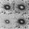 |
Fig. 7 Illustration of the comparative depth of the CFHT and Euclid Perseus cluster observations (the featured galaxy is PGC 12254). This image indicates that our ground-based optical data (r-band here) match the Euclid data well, both for compact sources and extended emission. The detection becomes challenging from the ground towards the NIR, where the Earth sky brightness increases rapidly (CFHT z-band observations versus Euclid HE-band here). The FoV per panel is 4′ by 4′. |
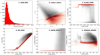 |
Fig. 8 Diagnostics used for star-galaxy separation. A source is classified as a star if it fulfils at least four selection criteria. The panels illustrate (1) the distance with the matched Gaia-DR3 stars; (2) the colour–colour diagnostic; (3) the stellarity criterion provided by SourceExtractor; (4) the relation between the magnitude in the Kron-aperture and the maximum surface brightness; (5) the size of the objects; and (6) the SPREAD_MODEL sequence for point-like objects. The objects selected in each criterion are highlighted in red. |
4.1 Star/galaxy separation
The availability of colours and morphological parameters from SourceExtractor1 allowed us to perform a thorough star-galaxy separation, combining different methods, with limits identified looking at positions of the matched SDSS and Gaia stars and extrapolating to fainter magnitudes. We applied the following six criteria (see e.g. Temporin et al. 2008; Estrada et al. 2023, for similar combinations of criteria):
match with Gaia DR3 (Gaia Collaboration 2016, 2023) stars: candidate stars are identified within a search radius of
![$\[0^{\prime \prime}_\cdot3\]$](/articles/aa/full_html/2025/05/aa50808-24/aa50808-24-eq10.png) ;
;colour–colour (g − z) versus (z − HE) diagram: with candidate stars characterised by (z − HE) < 0.3(g − z) − 0.2 (similar to the well known BzK criterion by Daddi et al. 2004);
stellarity classifier: high probability provided by CLASS_STAR, with CLASS_STAR > 0.95 in IE if MAG_AUTO > 16 or CLASS_STAR > 0.80 if MAG_AUTO ≤ 16 to include saturated objects;
compactness: the maximum surface brightness to be MU_MAX < 14.5 in IE if MAG_AUTO < 16 (to include saturated objects) or MU_MAX < 0.9 MAG_AUTO if MAG_AUTO > 16;
small size: KRON_RADIUS = 3.5 px in IE, corresponding to the minimum aperture adopted in SourceExtractor;
comparison with local PSF: SPREAD_MODEL < 0.01 in IE (see also Massari et al. 2025), with SPREAD_MODEL being a SourceExtractor parameter that compares the objects with the local PSF model, and providing values close to zero for point sources, positive for extended sources, and negative for detections smaller than the PSF.
The criteria and their selection regions are illustrated in Fig. 8, where in some of the panels the transition to bright saturated objects is producing discontinuities.
We considered as stars the objects fulfilling at least four of the six above criteria. To validate the procedure, we verified that all the objects identified as stars in SDSS are included in our sample. The final number of selected candidate stars is 49 922 and their number counts are in fairly good agreement with the Besançon model of stellar population synthesis of the Galaxy (Robin et al. 2003; Czekaj 2012; Lagarde et al. 2021) as shown in Fig. 9. We observe a mild overestimate of our star number counts at magnitudes between mi = 15 and 19, that can be due to either misidentification of globular clusters or of compact galaxies. Very compact or nucleated galaxies could be classified as stars with the above criteria: we verified that among the sample of dwarf galaxies in Marleau et al. (2025), only 4 out of 1100 were incorrectly assigned to the sample of stars candidates. The above validations indicate that the combination of criteria for star-galaxy separation is effective out to faint magnitudes, at the same time avoiding the failure of some criteria because of saturation issues. The remaining 212 975 objects are considered as galaxies in the following analysis.
4.2 Milky Way extinction
Intrinsic fluxes are derived by correcting for the MW extinction, which is significant in the Perseus FoV (see also Marleau et al. 2025). We adopted the Planck 2013 (Planck Collaboration XI 2014) dust opacity map2, from which we extracted the values of the colour excess E(B − V) to be associated to each galaxy in our catalogue. The colour excess is related to the magnitude absorbed at different wavelength through the MW extinction curve k(λ) = A(λ)/E(B − V) = RV A(λ)/AV, where A(λ) and AV are the magnitudes attenuated at the wavelength λ and in the V filter. We used the extinction curve by Gordon et al. (2023), assuming the extinction ratio RV = 3.1.
Since the extinction depends on the wavelength and can vary substantially, especially in the UV, the exact derivation of the absorbed magnitude in broad-band photometry depends also on the shape of the spectral energy distribution (SED) of the observed object (e.g. Galametz et al. 2017). The correction process is implemented in a consistent way in Phosphoros (Paltani et al. in prep.), the photometric redshift code used in Sect. 4.3, while we employed the SED of a 5700 K blackbody to derive an average correction in all the other cases. To this aim we derived a factor cx to derive the intrinsic magnitude in a filter x as mint = mobs − cxE(B − V). This parameter has been derived including the above ingredients and the total transmission of the filters Rx(λ) represented in Fig. 2 multiplied by λ to take into account the photon transmission:
![$\[c_x=2.5 ~\log _{10} \frac{\int R_x(\lambda) ~\lambda~ F_{\text {BB5700 }}(\lambda) 10^{0.4 k(\lambda)} ~\mathrm{d} \lambda}{\int R_x(\lambda) ~\lambda ~F_{\text {BB5700 }}(\lambda) ~\mathrm{d} \lambda}.\]$](/articles/aa/full_html/2025/05/aa50808-24/aa50808-24-eq11.png) (1)
(1)
The values we obtained are cx = 4.633, 3.552, 2.516, 1.919, 1.487, 2.122, 1.066, 0.726, and 0.470 in the u, g, r, i, z, IE, YE, JE, and HE bands, respectively. Given that the E(B − V) values range from 0.12 to 0.20, the magnitudes absorbed in the IE band range from 0.255 to 0.424. These corrections have been implemented for the objects not classified as stars.
The galaxy number counts compared to COSMOS2020 (Weaver et al. 2022) and literature data are shown in Fig. 10. Overall we see a quite good agreement in the whole range of optical and NIR magnitudes. At bright magnitudes the COSMOS2020 catalogue is incomplete because the COSMOS field was chosen to explore the distant Universe, while the decrement at faint magnitudes is due to the incompleteness beyond the limiting magnitudes.
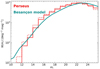 |
Fig. 9 Number counts in the MAG_AUTO iCFHT band compared to the Besançon model rendition in the same filter. The reference counts have been extracted at the centre of the Perseus field in an area of 1 deg2 and compared to the number counts of stars selected with the multiple criteria method. The solid histogram refers to the data not corrected for MW extinction, while the dashed histogram represents the corrected iCFHT. |
4.3 Full-sample photometric redshifts
The photometric parameters of all the detected sources have been extracted using SourceExtractor on the compact-source stacks. This extraction pipeline has been run in dual mode on all the CFHT and Euclid NISP images, while in an independent mode on the Euclid VIS image, producing a different number of detected sources, as mentioned in Sect. 4.
The photometric redshifts of all sources identified as galaxies in Sect. 4 have been derived using the SED fitting code Phosphoros3 (Euclid Collaboration: Desprez et al. 2020), and are denoted as zphot hereafter. We used the CFHT broad bands and NISP for which all the parameters have been derived within the same Kron aperture determined by SourceExtractor in the χ2 image (see Sect. 4), while the VIS catalogue has been derived separately, so as not to lose its superior resolution. For this reason the VIS photometry has not been used to derive photometric redshifts.
Photometric redshifts have been derived by comparing the observed photometry values with that derived from the templates used in COSMOS (Ilbert et al. 2009), suitable for high-redshift galaxies that need to be separated from the potential Perseus members. In template SED fitting, a grid of model photometry is generated for plausible amounts of the internal dust attenuation and the redshift, with finer redshift steps (three equally spaced binning schemes in three redshift ranges) at very low redshift. However, photometric redshifts derived from template fitting techniques inherently face challenges at low redshifts. The key features used to estimate the distance of a galaxy from broadband photometry are the slope of the SED and spectral breaks, notably the 4000 Å break. While this break can be bracketed by the u and g filters out to a redshift z ≃ 0.35, degeneracy in the properties regulating the slope of the blue part of the SED result in poor constraints at low redshift with this combination of broad-band filters.
Promising improvements have been obtained for bright and resolved objects when using machine-learning techniques complementing the flux measurements with the images (Treyer et al. 2024). Nonetheless template-fitting methods are still required for faint galaxies for which no training sample is available.
A compromise between the need to remove high-z sources without rejecting potential members has been achieved with the use of a prior. The luminosity function prior, implemented in a fully Bayesian manner in Phosphoros, adjusts the likelihood when a degenerate probability distribution function is encountered based on the probability of a galaxy having a given luminosity at the photometric redshift. For our prior, we adopted the LF in the B band derived by Giallongo et al. (2005) at a redshift of approximately 1.2 (chosen to avoid overly constraining the bright local galaxies).
The robustness of these photometric redshifts is tested here by comparing their values to those of the spectroscopic redshifts, where available, within the observed field (130 objects, see Fig. 11)4. Despite the very limited number of objects (the ERO Perseus field is the first deep field ever observed within the Euclid photometric bands), Fig. 11 shows that a selection of zphot ≲ 0.1 is appropriate to include all galaxies identified as Perseus members, thanks to their spectroscopic redshift. With this cut, the contamination of background galaxies is 17/130 (≃13%) with a limit on spectroscopic redshift (zspec ≲ 0.03) for cluster membership. We thus rejected in the following analysis all sources with zphot > 0.1.
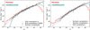 |
Fig. 10 Number counts of galaxies in the Perseus field compared to COSMOS2020 in HE and iCFHT, both corrected for MW extinction. Other data from the literature are taken from (Driver et al. 2016, D16), while the Durham Cosmology Group’s counts are from the compilation available at the dedicated web page (http://star-www.dur.ac.uk/~nm/pubhtml/counts/counts.html). Left: HE number counts. The COSMOS (from the Farmer catalogue described in Weaver et al. 2022, after removing masked regions and objects classified as stars) counts are derived from UltraVISTA H-band magnitudes converted to HE using the equation D. 22 in Euclid Collaboration: Schirmer et al. (2023, solid dark cyan line). Perseus galaxy number counts in HE are shown as a solid red line. The excess in the bright number counts can be explained by the contribution of Perseus cluster members. Right: i-band number counts. The COSMOS2020 data are from the HSC i-band, Perseus magnitudes are IE (red solid line). The same excess at bright magnitudes is also observed. |
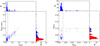 |
Fig. 11 Left: Comparison between the SDSS photometric redshift and the spectroscopic one for targets located within R ≤ r200 in the Perseus cluster with an r-band magnitude r ≲ 17.7. Right: Comparison between the photometric redshifts derived with Phosphoros and the spectroscopic ones for targets located within the Euclid field of the Perseus cluster (R ≤ 0.25 r200). The vertical black dotted line shows the adopted limit in spectroscopic redshift used for identifying Perseus members [zspec ≲ 0.03, corresponding to Vc + 3.5 σc = (5258 + 3.5 × 1040) km s−1]. The green dashed line shows the limit in photometric redshift to identify potential cluster candidates [zphot,SDSs ≲ 0.1, left; zphot ≲ 0.1, right]. The upper and right histograms show the spectroscopic and photometric redshift distribution, respectively, for all galaxies and for those objects classified as cluster members using their spectroscopic redshift (zspec ≲ 0.03, red). |
5 Identification of cluster galaxies
The major challenge in the determination of the LF and SMF in nearby clusters of galaxies is the accurate identification of all cluster members down to a given magnitude limit. The different criteria used to identify cluster members should also maximise the completeness and minimise the contamination of foreground and background sources. The analysis presented in this work is based on a selection performed on the VIS data, which are of higher image quality in terms of sensitivity and angular resolution than the NISP data. We also limit the identification of cluster members to resolved systems, that is, to objects with an optical extension exceeding 56 pc (corresponding to the size of the FWHM in VIS, ![$\[0^{\prime \prime}_\cdot16\]$](/articles/aa/full_html/2025/05/aa50808-24/aa50808-24-eq12.png) , see Sect. 3.1). We discuss in a following section how this assumption can affect the results. This identification of members without spectroscopic redshifts is first based on morphological arguments, as successfully done in the Virgo cluster (e.g. Binggeli et al. 1985). Despite the greater distance to Perseus (72 Mpc versus 16.5 Mpc for Virgo), this is possible thanks to the excellent image quality of the Euclid data versus the ground-based imaging data of the NGVS in terms of angular resolution (FWHM in the i band is approximately
, see Sect. 3.1). We discuss in a following section how this assumption can affect the results. This identification of members without spectroscopic redshifts is first based on morphological arguments, as successfully done in the Virgo cluster (e.g. Binggeli et al. 1985). Despite the greater distance to Perseus (72 Mpc versus 16.5 Mpc for Virgo), this is possible thanks to the excellent image quality of the Euclid data versus the ground-based imaging data of the NGVS in terms of angular resolution (FWHM in the i band is approximately ![$\[0^{\prime \prime}_\cdot6\]$](/articles/aa/full_html/2025/05/aa50808-24/aa50808-24-eq13.png) , Ferrarese et al. 2012, versus
, Ferrarese et al. 2012, versus ![$\[0^{\prime \prime}_\cdot16\]$](/articles/aa/full_html/2025/05/aa50808-24/aa50808-24-eq14.png) in Perseus) and sensitivity to LSB features (μg = 29.0 mag arcsec−2 versus μIE = 30.1 mag arcsec−2 in Perseus). More stringent statistical and quantitative methods, based on selected scaling relations, are then applied to reject background systems and reduce incompleteness. To this aim we adopt the methodology used by Ferrarese et al. (2016, 2020) and Boselli et al. (2016), which has already been shown to be efficient in the Virgo cluster.
in Perseus) and sensitivity to LSB features (μg = 29.0 mag arcsec−2 versus μIE = 30.1 mag arcsec−2 in Perseus). More stringent statistical and quantitative methods, based on selected scaling relations, are then applied to reject background systems and reduce incompleteness. To this aim we adopt the methodology used by Ferrarese et al. (2016, 2020) and Boselli et al. (2016), which has already been shown to be efficient in the Virgo cluster.
The sample of galaxies analysed in this work is the combination of dwarf Perseus members described in Marleau et al. (2025) and the bright Perseus members (Mondelin et al. in prep.). The process that lead to the final catalogue of Perseus members is illustrated in the flowchart in Fig. 12.
The structural parameters used in the present analysis have been derived with AutoProf and AstroPhot, as briefly described in Appendix B. These two tools, while demonstrating equivalent effectiveness for isolated galaxies, complement each other well within the highly diverse environment of the Perseus cluster. Together, they deliver quality photometry for all types of galaxy. For a detailed analysis see Marleau et al. (2025) and Mondelin et al. (in prep.).
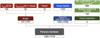 |
Fig. 12 Flowchart representing the process of selecting cluster members. The red branch in the left represents the steps described in Sect. 5.1. The blue boxes are for the dwarf galaxies in Sect. 5.2, and in green we illustrate the different steps we followed to check for any possible additional member, starting from the SourceExtractor (SE on the flowchart) catalogue, discussed in Sect. 5.4. Numbers in italic and between parentheses represent the galaxies brighter than the completeness limit we adopted for the LF, M(IE) ≤ −11.33. |
5.1 Bright members
Bright galaxies were first selected according to their spectroscopic redshifts taken from the SDSS catalogue5, but also from the NASA Extragalactic Database6. We defined as cluster members those with 0.005 ≤ zspec ≤ 0.03, with the higher limit corresponding to Vc + 3.5 σc7. The spectroscopic selection resulted in 105 galaxies.
SDSS photometric redshifts are available for galaxies with r-band magnitudes brighter than around 21 (Csabai et al. 2003, 2007). Being trained on a large sample of galaxies mainly located in the local Universe, these photometric redshifts are optimised to identify local systems with good accuracy8. This is particularly true for galaxies with magnitudes r ≲ 17.7, the redshift completeness limit of SDSS. Figure 11 shows the relationship between the SDSS photometric redshifts and the spectroscopic redshifts for all galaxies with available spectra within the Perseus cluster (R < r200). A cut in zphot(SDSS) ≲ 0.05 secures an identification of 88% of the spectroscopically identified cluster members defined as above, with a minor contamination (5%). However, given the bias and the dispersion characterising photometric redshifts in the low-z regime, we preferred to maximise the completeness, using a cut in zphot(SDSS) ≲ 0.10, reaching a completeness of 99% at the cost of an increase in the contamination (24%). We therefore selected all sources within the footprint of the Euclid observations with zphot(SDSS) ≲ 0.10 and r ≲ 17.7, and identified members using morphological criteria. We excluded from the analysis all stars and objects already identified as Perseus members or galaxies with spectroscopic redshifts zspec > 0.03. These candidates were then visually inspected and we confirmed as cluster members those galaxies with sizes exceeding several arcseconds and/or displaying visible substructures such as those observed in spectroscopically confirmed members. This includes another 20 objects. Finally, we reviewed the entire VIS image, overlaying the cluster member source catalogue to ensure no bright galaxies with sizes of a few arcseconds were overlooked, and identified another 12 members. Combining the three selection methods – spectroscopic, photometric, and visual – we obtained a sample of 137 bright cluster members.
5.2 Dwarf members
The dwarf systems have been identified as cluster members after visual inspection of the VIS and VIS+NISP colour images performed by seven independent (human) classifiers. A detailed description of the criteria used to identify and select the dwarf galaxy candidates, as well as the comparison with other samples of dwarf systems in this cluster, can be found in Marleau et al. (2025). Briefly, galaxies are identified as members whenever they have morphological properties such as diffuse and extended emission, colours, and structural properties (resolved nuclei, bars, spiral arms, etc.) as those observed in spectroscopically confirmed Perseus members. We recall that cluster membership based on morphological classification has been successfully used in the past (e.g. Binggeli et al. 1985, VCC catalogue), also in massive clusters such as Coma (Michard & Andreon 2008) and Perseus (Wittmann et al. 2019). A total of 1100 dwarf galaxies were counted. We then shift our focus to galaxies located at the periphery of the FoV captured by both the NISP and VIS instruments. The two FoVs do not perfectly overlap, as depicted in Cuillandre et al. (2025), causing some sky coverage area lost on either instrument. For the LF analysis requiring all photometric bands, we concentrate on the shared FoV between VIS and NISP. Thus, 17 dwarf galaxies were excluded from the catalogue of cluster members.
In the following analysis, we refer to galaxies identified using purely morphological criteria, either for the bright or the dwarf samples, as the ‘visual catalogue’. Adding those spectroscopically confirmed galaxies, the bright plus dwarf sample is composed of 1220 galaxies.
5.3 Completeness
We derived the catalogue of bright and dwarf galaxies through exhaustive visual scrutiny of the entire dataset, initially detecting galaxies from the high-resolution VIS IE-band image and using the VIS+NISP colour images for additional verification (Marleau et al. 2025). The manageable size of our Euclid FoV for the Perseus cluster allows this approach over a fully automated method (e.g. Ferrarese et al. 2020). This method ensures a comprehensive review of cluster galaxy candidates, yielding a nearly complete sample, although mastering the completeness function is essential to correct the LF.
Completeness loss occurs due to the finite depth of the dataset or the complex nature of the observed field, where high star density and dense interstellar matter, along with large, bright cluster galaxies, can obscure fainter galaxies. About 10% of the Euclid Perseus field is occupied by bright sources, complicating the detection process.
To analyse completeness, we simulated the injection of dwarf galaxies into the original Euclid IE image. We selected three square areas, each 1000″ × 1000″, representing a significant 44% of the whole image, while encompassing the three most diverse environments: one centred on the cluster core rich in large galaxies (Region 1); one in an area heavily affected by Galactic cirrus (Region 3); and one relatively free of these complexities, but with similar stellar density (Region 2). Figure 13 illustrates these regions, highlighting the variability in environmental conditions that affect light detection.
The initial step involved selecting an automated detection method capable of accurately identifying the majority of galaxies in our catalogue of members, while excluding most sources that do not share their morphological characteristics. This strategy ensures that the detection method can be confidently used to identify injected simulated galaxies without mistaking them for other compact sources.
Testing different image-filtering techniques revealed that the ring filter, recommended by Secker (1995) and Ferrarese et al. (2020) for this specific task, is near to optimal9. We utilised the background map created by the ICL team (Kluge et al. 2025) aimed at detecting compact sources. The parameters for the ring filter were set with an inner radius of 2 pixels and an outer radius of 4 pixels, with the VIS FWHM at 1.6 pixels. The resulting smoothed background map effectively meets our requirements for detecting faint extended structures.
Visual inspection showed that all faint galaxies (IE > 16) were significantly enhanced. SourceExtractor (Bertin & Arnouts 1996) was then configured to detect only objects exceeding a size of 500 pixels (DETECT_MINAREA), with a detection threshold above 2 σ (DETECT_THRESH), and using a 64-pixel mesh size (BACK_SIZE), along with a moderate smoothing filter (BACK_FILTERSIZE = 3) for internal background subtraction.
This approach achieved a recovery rate of 93% for all faint galaxies in our catalogue, which have a limited angular size on the sky and remain unaffected by the internal sky background subtraction – ensuring they are not partially erased. Figure 14 demonstrates these steps, from the original image through the ring-filtered version to the SourceExtractor segmentation map, confirming the effective detection of all dwarf galaxies.
While the SourceExtractor measurements are not as precise as those from AutoProf/AstroPhot for determining the total magnitude of these peculiar objects – being within 0.5 magnitude of accuracy – they still enable a fully automated method just for testing completeness. This is done by injecting simulated galaxies and verifying how many are successfully identified in the extracted catalogue10.
To ensure comprehensive statistics, we injected each simulated galaxy onto a grid every 25″ in both the x and y directions across our observational regions, resulting in 400 injections per region, totalling 1200 injections for each simulated galaxy. This process was replicated for 817 galaxies spanning nine magnitude bins from IE = 16 to IE = 24. Initially, we analyse the primary physical parameters of the dwarfs in our visual catalogue on the IE image: Sérsic index; effective radius Re; surface brightness at Re (Ie); ellipticity; position angle; and total magnitude IE (Marleau et al. 2025). An average of 90 galaxies per magnitude bin was sampled using a multivariate Gaussian fit to reflect the actual distribution of these parameters among the dwarf population.
Figure 15 illustrates the correlations between these six parameters in red. The total magnitude IE, which is closely linked to the Sérsic index n, Ie, and Re, was included for demonstration only, and was not directly used in the simulations. Instead, it was derived from n, Ie, Re, and the ellipticity. The blue dots in Fig. 15 represent the randomised parameters drawn to accurately depict the actual dwarf population in the Perseus cluster.
We utilised the image simulation tool makeimage from the Imfit package (Erwin 2015) to generate 817 250 pixel × 250 pixel stamps based on our five drawn parameters. The largest dwarfs in our visual catalogue do not exceed 20″ in diameter, as highlighted in the sub-panel for Re in Fig. 15.
Each stamp is replicated 400 times in a 20 × 20 grid and inserted into each of the three ring-filtered regions to streamline the process and conserve computing resources. This method is effective since these stamps, featuring flat and featureless profiles, are minimally impacted by the tight ring filter, with differences at the percent level.
There is no need to randomise the injection positions due to the automated detection scheme employed. Figure 16 demonstrates this process, where the SourceExtractor segmentation map shows that the simulated galaxies are often successfully recovered (indicated by red circles). Figure 17 displays two instances where recovery failed due to overlaps with a bright star and a background galaxy.
The recovery level, which assesses completeness for each galaxy, is determined by automatically comparing the extracted catalogue with the values in a catalogue generated by SourceExtractor from simulations using the same parameters. We use a matching radius of 1″, and a galaxy is considered lost if its recovered magnitude deviates by 5 σ from the expected value, based on the dispersion observed across 400 measurements without injections.
Overall, 980 400 simulated galaxies were processed by SourceExtractor to generate three completeness measurements per galaxy, corresponding to each of the three regions. To validate the method, we ran a matching code for each galaxy against the SourceExtractor catalogue produced for the three regions without any injected galaxies, ensuring that our tests were not influenced by existing sky data. The negligible matching level of 0.4% confirms that the completeness values accurately reflect the ability to recover the injected simulated galaxies, free from background contamination.
The correlation of the 2451 measurements with our key parameters is detailed in Fig. 18. Clear expected trends are evident with respect to the Sérsic index, Re, but it is the total magnitude Ie that shows the strongest correlation. We expand on this specific completeness relationship with the lower right panel of Fig. 18 turning into Fig. 19, now focusing on absolute magnitudes M(IE).
A polynomial fit (dashed red line) illustrates a slight decline in completeness from M(IE) = −18 to M(IE) = −12, beyond which completeness rapidly decreases, hitting 50% at M(IE) = −11 and nearly 12% at M(IE) = −10. Comparisons across the three regions (Fig. 13) reveal that only the presence of large galaxies in Region 1 slightly impacts completeness across all magnitude bins, reducing it by 7%. In consequence we adopt a unique completeness correction across the entire IE range. This polynomial fit in Fig. 19 incorporates all simulated dwarf measurements and thus represents the median completeness across the entire image, it is the adopted completeness function for this work.
The faintest members of the bright galaxies in our catalogue were tested using the same method as the dwarfs, with results depicted in green on Fig. 19. This approach is effective primarily for galaxies in the faintest magnitude bin at M(IE) = −18, where galaxies are also more compact. To accommodate their size and prevent truncation, the simulation and injection grid was expanded from 250 × 250 to 1000 pixels × 1000 pixels.
This testing shows that completeness stands at 96% for nondwarf galaxies at M(IE) = −18. However, completeness quickly decreases for brighter and more extended galaxies because our dwarf-focused measurement method unintentionally suppresses flux due to SourceExtractor’s background subtraction being influenced by the galaxy itself. This was visually confirmed, as even the faintest bright galaxies are distinguishable when near a star or adjacent to a larger galaxy. Given the few faint non-dwarf galaxies in the M(IE) = −18 bin, it is evident that a completeness correction for the luminosity function (LF) is unnecessary for the bright galaxies (M(IE) > −18).
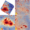 |
Fig. 13 Perseus field divided into three regions of 10 000 pixels × 10 000 pixels each (1000″ on a side) to investigate completeness under various conditions. Region 1 contains large galaxies, Region 2 has a regular field density composed of background galaxies and stars; and Region 3 shows Galactic cirrus. The Galactic cirrus manifests itself as a faint orange haze in frame 3, with the top-left thumbnail displaying an enhanced version of the image that highlights extended diffuse emission, cirrus, and intracluster light. Collectively, these three representative regions cover 44% of the total area. In all images, north is oriented upwards, and east is to the left. |
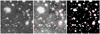 |
Fig. 14 Left: Section of the original VIS image (900 pixels × 900 pixels, 90″ on the side) displaying standard features, specifically extended cluster galaxies, stars, background galaxies, and optical ghosts near bright stars, which appear as faint round structures. Middle: Ring-filtered version enhancing extended sources and removing compact ones. The red circles (10″ in diameter) mark the dwarfs from our catalogue of members. Right: SourceExtractor segmentation map confirming detection of all dwarfs and maintaining a low count of other detected sources. |
5.4 Other possible members
The selection described in Sects. 5.1 and 5.2, which is mainly based on spectroscopic redshift, photometric redshift from SDSS, and morphological criteria, might be contaminated by a few background sources and at the same time might miss faint compact objects discarded for their small angular size. To quantify these possible effects we extend the analysis to all the sources detected by SourceExtractor within the field, described in Sect. 4.
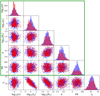 |
Fig. 15 Fits to model parameters for dwarf galaxies. A multivariate Gaussian fit (blue dots) was applied to the dwarf sample from the visual catalogue (red dots), ensuring the five defining parameters per galaxy – Sérsic index n, surface brightness Ie at the effective radius Re, ellipticity e, and position angle PA, indicated in the green box – are weighted proportionally to their occurrence in the real data. The total magnitude IE, dependent on Sérsic index, Ie, and Re, is not used in the simulation. |
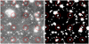 |
Fig. 16 Injection of simulated galaxies. Left: Simulated IE = 22.4 dwarf galaxy with specific physical parameters (Sérsic index = 0.61, Ie = 0.49 ADU per pixel, Re = 18.10 pixels, ellipticity = 0.14, and position angle = 72°) injected into a 250 pixel × 250 pixel grid (marked by red circles). Right: SourceExtractor segmentation map showing successful recovery of most injected sources. This example clearly demonstrates how completeness is compromised by crowding from nearby stars and galaxies. The image area is the same as in Fig. 14. |
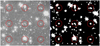 |
Fig. 17 Image of a 75″ wide area featuring nine injected dwarf galaxies (the same as shown in Fig. 16). Two galaxies are not recovered. The centre top red circle overlaps with a background galaxy, and the centre bottom overlaps with a bright star. The segmentation map on the right displays a single polygon at the location of each simulated dwarf, highlighting where recoveries succeeded and where they were hindered by overlapping objects. |
5.4.1 Scaling relations for the full SourceExtractor catalogue
Following Boselli et al. (2016) we use the output parameters of SourceExtractor to construct several scaling relations to identify all possible cluster members. Given that the completeness test shown in Sect. 5.3 has indicated that the catalogue is approximately 50% complete at IE ≃ 22.96 (including a mean Galactic attenuation of AIE ≃ 0.33), we limit the analysis to all detected sources satisfying this magnitude limit. These are 20 456 galaxies, of which 899 with zphot ≤ 0.1 are not already included in the bright or dwarf samples, and 30 222 stars.
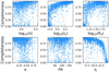 |
Fig. 18 Completeness covariance with respect to the main physical parameters. The total magnitude IE (lower right), which is derived from the Sérsic index n, the effective radius Re, Ie the surface brightness at Re, and the ellipticity e, shows the tightest relation to completeness. |
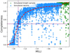 |
Fig. 19 Completeness estimates. The completeness of the Perseus dwarf galaxies is depicted in blue, based on 980 400 individual injections across three distinct Perseus regions, each containing 400 samples from each of the 817 simulated galaxies, resulting in 2451 completeness measurements shown on this plot. The dashed red line (a polynomial fit based on the median values) shows that completeness begins to decline at M(IE) = −12, dropping to 50% (horizontal dashed line) at −10.9. The green data points illustrate that even the faintest of our bright galaxy samples achieve 96% completeness when simulated similarly to the dwarfs, with completeness approaching 100% at M(IE) = −19. For brighter and larger galaxies, the testing method used here is not ideally suited, leading to an apparent drop in completeness (green dots on the right). However, our catalogue achieves 100% completeness for all bright galaxies. |
Surface brightness versus total magnitude
Figure 20 shows the relation between the mean model effective brightness (MU_MEAN_MODEL, representing the mean effective surface brightness above the background from the model-fitting photometry) and the proxy for the total magnitude (MAG_AUTO in the versus) both corrected for dust attenuation using the extinction law from Gordon et al. (2023) and the Planck 2013 dust map (Planck Collaboration XI 2014), as described in Marleau et al. (2025).
As already noticed in Boselli et al. (2016), this scaling relation well segregates stars from galaxies. If we arbitrarily define the relation ⟨μIE⟩ = 0.783 IE + 3 mag arcsec−2, indicated by the black solid line in Fig. 20, we notice that 217/30 224 (0.7%) of the sources identified as stars using four, five, or six independent methods (as described in Sect. 4) are located below this relation, while 886/899 of the cluster members (spectroscopically confirmed or visually identified and included in the SourceExtractor catalogue11) are above it (98.5% completeness). It is thus likely that the large majority of the sources with zphot smaller than or equal to 0.1 (green dots) located below this line are misclassified stars that can be removed. We thus adopted this cut to exclude the largest number of possible stars from the following analysis. Since some of them might still be present, we identify them by visual inspection at different stages of the selection using scaling relations.
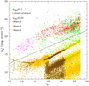 |
Fig. 20 Relation between the mean versus model effective surface brightness and the total magnitude for all sources in the full SourceExtractor catalogue with IE ≤ 22.96. Brown, orange, and yellow dots are for targets classified as stars consistently by six, five, and four independent criteria, respectively. Green dots are for galaxies with photometric redshifts from Phosphoros zphot ≤ 0.1, red dots for optically identified cluster members, and magenta dots for spectroscopically confirmed cluster members (zspec ≲ 0.03). The black solid line (⟨μIE⟩ = 0.783 IE + 3 mag arcsec−2) delimits the region where most (13/899, 1.4%) of the spectroscopically and visually identified members are located. |
Colour–colour and colour–magnitude relations
Again, following Boselli et al. (2016) we construct other diagnostic diagrams to identify background galaxies from those located within the Perseus cluster. Figure 21 shows the i − HE versus g − HE colour–colour diagram for the galaxies satisfying the previous criteria (i.e. with zphot ≲ 0.1 and identified as galaxies in Fig. 20). The figure compares the distribution of these objects to that of the galaxies identified as members using morphological criteria.
The spectroscopically and visually identified cluster members are well located along a very tight relation (see Figure 21), while the galaxies with a photometric redshift zphot ≲ 0.1 follow the same relation but with a substantially larger scatter, with on average redder i − HE colours than cluster members. Their distribution within this diagram suggests that some of them are background galaxies and can thus be removed from the following analysis. We did so by removing all objects located outside ±3 σ of the best-fit relation. We also excluded all objects with i − HE > 1.1, since all the massive and spectroscopically confirmed galaxies of the cluster have colours bluer than this value. This choice is justified by the fact that possible members are likely low-luminosity metal-poor objects, thus their colour is bluer than that of massive cluster members. The resulting sample of potential members missing from the catalogue of bright and dwarf galaxies drops to 300 candidates.
Finally, as is common in the literature, we use a colour–magnitude relation (e.g. Bower et al. 1992; Aguerri et al. 2020, for Perseus), g − HE versus IE in this case, to further reject background galaxies from the sample of potential members (Fig. 21). Most spectroscopically or visually identified cluster members are located along a tight colour–magnitude relation, as expected for a galaxy population highly dominated by quiescent early-type systems. Those located 3 σ above the relation12 (redder colours, 15 objects) are either galaxies with uncertain colours as given by SourceExtractor, which is optimised to derive photometric parameters for point sources, or background galaxies. Those located below the relation (16) are mainly background objects or star-forming systems, rare but still present in massive clusters of galaxies (e.g. Gavazzi et al. 2010; Boselli et al. 2014). Indeed, visual inspection of those already identified as cluster members show a spiral/irregular morphology typical of star-forming systems, some of which also host star-forming regions evident in the narrow-band Hα image (see next section). After removing the objects located above the colour–magnitude relation, the sample of potential members not included in our catalogue drops to 285 objects, 16 of which are located >3 σ below the relation traced by quiescent, early-type systems.
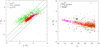 |
Fig. 21 Left: colour–colour diagram of i − HE versus g − HE for all sources in the full SourceExtractor catalogue. The points represent the objects with IE ≤ 22.96 identified as galaxies in Fig. 20 with zphot ≲ 0.1 (green dots), and optically identified (red dots) or spectroscopically confirmed (magenta dots) cluster members (zspec ≲ 0.03). Filled dots are for galaxies with uncertainty in the colour larger than 0.1 mag. The black dashed line shows the bisector fit to the data, (i − HE) = (0.99 ± 0.02) × (g − HE) − (1.06 ± 0.01), σ = 0.26, for galaxies with a colour uncertainty σcol ≲ 0.1, while the solid lines delimit the region within the 3 σ dispersion of the relation, where 99.7% of the spectroscopically and visually identified members are located. The black solid horizontal line shows the upper limit in colour observed in the spectroscopically confirmed cluster members (i − HE < 1.1). Right: colour–magnitude relation of i − HE versus IE for the same sample of galaxies but limited to those objects identified as potential cluster members in the i − HE versus g − HE colour–colour diagram (left panel). Galaxies are identified using the same symbols, with the exception of green dots within black circles, which are systems lying > 3 σ from the mean colour–magnitude relation, where 99.7% of the spectroscopically and visually identified cluster members are located. Those located below the colour–magnitude relation are possible star-forming cluster members. |
Hα+[N II] excess
Galaxies located more than 3 σ below the colour–magnitude relation traced by quiescent early-type systems (16 objects) are either blue background galaxies or star-forming systems within the Perseus cluster. In this second case, their ongoing starformation activity would produce ionising radiation detectable in the Balmer Hα emission line at 6563 Å. If present, this line emission can be detected in the narrow-band Hα image of the cluster, which has been taken within a filter covering the velocity range 4660 km s−1 ≲ vhel ≲ 9600 km s−1 thus perfectly matching that of the cluster. We visually inspected the continuum-subtracted images of these objects, and found that only one of the 16 objects has detectable Hα+[N II] emission. This source, however, is discarded because it is associated with the perturbed gas of the galaxy UGC 2665, which is already included among the spectroscopically confirmed Perseus members. The lack of any Hα+[N II] in the remaining 15 objects indicates that they are all background systems, which are thus excluded from the following analysis, producing a sample of 269 galaxies.
We then visually inspected all the remaining objects selected using the VIS IE-band images. Out of these, 67 are misclassified stars, seven are bright objects at the edge of the field where the image of the galaxy is truncated, 37 are problematic sources in low S/N regions at the periphery of the frame where only a few exposures are available, or sources close to very bright stars where the photometry cannot be accurately measured. One source is another part of the fragmented ram-pressure-stripped galaxy UGC 2665, four are different parts of two independent merging, star-forming systems. Since they do not have any associated emission in the Hα+[N II] continuum-subtracted image, these must be background systems. All 116 of these sources can be removed from the following analysis.
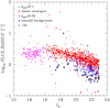 |
Fig. 22 Relation between the FLUX_RADIUS and the IE-band magnitude for all sources in the SourceExtractor catalogue with IE ≲ 22.96 identified as galaxies that satisfy the surface brightness-magnitude selection (Fig. 20), the colour–colour selection, and the colour–magnitude selection (Fig. 21, left and right panel) for potential cluster members. Filled and empty dots are for galaxies with uncertainty in the g − HE colour smaller or larger than 0.1, respectively. Magenta dots are for spectroscopically confirmed cluster members (zspec ≲ 0.03), red dots for optically identified members, and green dots potential members with zphot ≲ 0.1 after visual inspection of their VIS images. Blue dots are faint objects of small size considered as background systems. |
Size-magnitude relation
We then applied a new scaling relation, the size-magnitude relation, on the remaining 153 galaxies (see Fig. 22). Most of these are faint objects of small size when compared to those of the bright plus dwarf cluster catalogue. If we remove from the 153 those located at more than 3 σ from the scaling relation drawn by the cluster members in the visual catalogue, only 126 galaxies remain as potential candidates.
5.4.2 Visual inspection
A final visual inspection shows that the majority of the remaining 126 cluster candidates are tiny objects, with no obvious resolved structures or the presence of any globular clusters, suggesting that they could be members of the cluster. We thus consider them in the following analysis as background systems and we do not consider them in the determination of the luminosity and stellar mass functions.
To conclude, the selection based on SourceExtractor does not add any new objects; the final sample is therefore composed of 137 bright galaxies and 1083 dwarfs, for a total of 1220 objects inside the common FoV of VIS and NISP. This number drops to 1211 once the sample is cut to a completeness limit of IE ≲ 22.96 after correcting for the MW extinction.
Figure 23 illustrates the diversity of galaxy properties in the catalogue, with a cumulative light distribution showing that 90% of the light from the cluster originates from the top 7% of the most luminous galaxies. Fig. 24 is a map displaying the distribution of light across the cluster, superimposed on the adopted Planck dust map [average E(B − V) = 0.156].
5.5 Validation of cluster members
To further test the purity of the selected sample of cluster members, we determine some scaling relations but using a more accurate measure of different structural parameters derived for the Perseus galaxies by means of AutoProf, AstroPhot, and Galfit (Marleau et al. 2025, Mondelin et al. in prep.). Compared to those coming from SourceExtractor, where the different photometric parameters are derived automatically, here the ad-hoc extraction minimises the uncertainties, thus reducing any systematic scatter in the scaling relations. Figure 25 shows some typical scaling relations between several structural parameters (Sérsic index n, effective radius, central surface brightness, and mean effective surface brightness) as a function of the total magnitude. Surface brightness and magnitudes are corrected for Galactic dust attenuation as described in Marleau et al. (2025). Such scaling relations have been successfully used to identify cluster membership in Virgo by Ferrarese et al. (2020).
Figure 25 shows that all the selected galaxies are well distributed along tight relations, and consistently indicates that the selected galaxies are all likely cluster members. This suggests that the possible contamination of background galaxies in the selected catalogue, if present, is minimal and thus will not strongly affect the estimation of the LF.
5.6 The final catalogue
To conclude, after the different selection criteria adopted to identify cluster members we end up with 1172 galaxies of M(IE) ≲ −11 observed magnitude, or equivalently M(IE) ≲ −11.33 when corrected for Galactic attenuation, above a completeness limit of approximately 50%. Indeed, in this final step, 48 dwarf galaxies have corrected magnitudes M(IE) greater than −11.33. This is the sample of galaxies used to derive the LF.
To summarise, Perseus cluster members have been selected using the criteria illustrated in Fig. 12, and specifically morphology (from Marleau et al. 2024 and Mondelin et al. in prep.), or SDSS photometric redshift zSDSS ≤ 0.1. The possibility of adding missed members has been explored with a strict selection on the full catalogue of SourceExtractor detections with magnitude brighter than this limit, selecting sources satisfying the following criteria: Phosphoros photometric redshift zphot ≤ 0.1; ⟨μIE⟩ ≤ 0.783 IE + 3 mag arcsec−2; within 3 σ of the i − HE vs. g − HE, g − HE versus IE, and log10 FLUX_RADIUS vs. IE relation. This procedure would add only 123 possible cluster candidates, a number roughly comparable to the possible contamination of background objects selected using these standard relations. Thus, we did not include them in the following analysis. We recall that the completeness of the catalogue of members is ~90% (see Sect. 5.3). The one of possible Perseus members derived from the full catalogue using photometric redshifts and scaling relations is of the order of ~87%, 89% photometric redshifts, 98.3% the mean effective surface brightness versus total mag relation (Fig. 20), 99.7% in the colour–colour, colour–magnitude, and FLUX_RADIUS vs. magnitude relations (Figs. 21 and 22).
We also stress that the current selection, which is principally based on morphology, does not allow one to discriminate cluster members from foreground objects or from systems in the very close background from the cluster (vhel ≲ 12 000 km s−1). The possible contamination of these objects, however, is very marginal and can be estimated by integrating the i-band LF of the field derived at z = 0.1 by Blanton et al. (2003) using SDSS data in the range −25 ≤ Mi ≤ −11 and multiplying it by the sampled volume up to a distance of 170 Mpc (≃350 Mpc3, 15 objects in total).
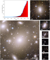 |
Fig. 23 Galaxy luminosity properties. Top left: Cumulative light distribution (blue line) for the Perseus cluster catalogue of 1220 galaxies, which reaches down to M(IE) = −10. The absolute magnitude of the galaxy at the centre of each image cutout is indicated in the IE band. While the 1083 dwarf galaxies dominate by number, 90% of the light in Perseus comes from the 83 galaxies brighter than M(IE) = −19.5 (the remaining 48 galaxies plus all dwarf galaxies account for just 10% of the light in Perseus). Image thumbnails: The top left diagram is illustrated with seven examples of relative brightness and physical size, all presented at the same pixel scale. The range spans from the giant elliptical NGC 1275 (bottom left), which alone contributes 10% of the light in Perseus, to a dwarf 12 magnitudes fainter (bottom right). The colour for each magnitude bin matches the colour used to represent galaxies on the map of Fig. 24. All dwarf galaxies are fainter than M(IE) = −18, while all other galaxies are brighter than M(IE) = −16. |
 |
Fig. 24 Perseus catalogue of 1220 galaxies plotted over the 0.7 deg2 sky coverage alongside the Planck dust map [average E(B − V) = 0.156]. The colour map for the galaxies is scaled from red to black according to the absolute magnitude ranging from M(IE) = −24 to −10 (Fig. 23). Measured ellipticity and angular size are depicted for the bright galaxies, while all 1083 dwarfs are represented as round dots, exaggerated in size relative to their physical dimensions. The three largest ellipses are NGC 1275 and NGC 1272 on the lower left, and NGC 1265 at the top. |
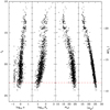 |
Fig. 25 Scaling relations between the Sérsic index n, the effective radius Re, the central surface brightness μIE, 0, and mean effective surface brightness within Re, ⟨μIE,e⟩, and the total magnitude measured using AutoProf/AstroPhot for all galaxies identified as cluster members. Magnitudes are corrected for Galactic attenuation. The red dashed line shows the 50% completeness of the sample, corresponding to M(IE) = −11.33, assuming a mean Galactic attenuation AIE = 0.33. The effective radius is in pixel units and surface brightness in mag arcsec−2. |
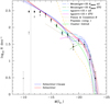 |
Fig. 26 Observed (grey dots) and corrected for completeness (black dots) IE-band LF derived excluding the three cD galaxies NGC 1275, NGC 1272, and NGC 1265. The solid red and blue lines and the associated dotted lines show the best-fit and 1 σ confidence regions of the Schechter and Schechter + Gaussian LF parametrisations, respectively. The vertical grey dashed line shows the 50% completeness limit. The two LFs are compared to those available in the literature for the Perseus cluster in the K band (Meusinger et al. 2020), in the r band (Aguerri et al. 2020), and in the B band (Penny & Conselice 2008), to the mean i-band LF of SDSS local clusters derived by Popesso et al. (2005) within 0.5 h−1 Mpc from the cluster centre, and to the Cluster-EAGLE simulations (Negri et al. 2022). The LFs of Perseus have been derived on different fractions of the cluster. They have been shifted to the IE band using the mean colour of galaxies in the cluster, and in the Y-axis direction to visually match the data. The best fit parameters are given in Table 3. |
6 The luminosity function
Luminosities and stellar masses used in this and the next sections have been derived for all identified Perseus members using the output of AutoProf and are thus total values. For presentation purposes, we derive a binned LF of the cluster by counting the number of objects per 1.0 dex bin of IE-band luminosity (corrected for Galactic extinction) and we correct it for completeness by dividing these numbers using the correction function shown in Fig. 19. The two LFs of the Perseus cluster, that have been measured within R ≲ 0.25 r200, are shown in Fig. 26.
The IE-band LF shows three clear regimes: a Gaussian distribution at the bright end with a clear dip at M(IE) ≃ −19; a steep rise out to M(IE) ≃ −14; and a flattening down to the completeness limit of M(IE) ≃ −11, with an abrupt decrease at fainter luminosity that is clearly due to incompleteness. The dip at M(IE) ≃ −19 seems real, since the number of objects in that magnitude bin (19) would need to be approximately double to reach those measured in the adjacent bins, which is impossible given that the survey is 100% complete at these luminosities. Indeed, the dip is 4.6 σ below the best-fit single Schechter function (see below), where σ is the Poisson uncertainty (for a critical discussion on the possible relation between incompleteness and the presence of the dip see Andreon et al. 2006). The flattening observed at M(IE) ≃ −14 might be partly due to incompleteness; however, the analysis presented in the previous sections suggests that the observed trend is real. Indeed, to keep the same slope observed in the −19 ≲ M(IE) ≲ −14 range (α ≃ −1.5, see below), the two following bins [M(IE) = −13 and −12] should be missing about 400 objects, which is very unlikely. The statistical analysis presented in Sect. 5 identified 123 potential cluster candidates that the selection might have missed, which includes the fainter magnitude bin M(IE) ≃ −11.
We fit the LF using a combination of parametric functions, specifically a Schechter (1976) function for faint objects and a Gaussian to reproduce the distribution of luminous galaxies:
![$\[\begin{aligned}\Phi(M) \mathrm{d} M= & \Phi_{\mathrm{S}}^* \\& \times\left\{0.4 ~\ln (10) 10^{-0.4\left(M-M_{\mathrm{S}}^*\right)\left(\alpha_{\mathrm{S}}+1\right)} \times ~\exp \left[-10^{-0.4\left(M-M_{\mathrm{S}}^*\right)}\right]\right. \\& \left.+A_{\mathrm{G}} ~\exp \left[-0.5\left(\frac{M-M_{\mathrm{G}}^*}{\sigma_{\mathrm{G}}}\right)^2\right]\right\} \mathrm{d} M,\end{aligned}\]$](/articles/aa/full_html/2025/05/aa50808-24/aa50808-24-eq40.png) (2)
(2)
where ![$\[\Phi_{\mathrm{S}}^{*}, M_{\mathrm{S}}^{*}\]$](/articles/aa/full_html/2025/05/aa50808-24/aa50808-24-eq41.png) , αS are the normalisation, the characteristic absolute magnitude and the faint-end slope of the Schechter function, while AG,
, αS are the normalisation, the characteristic absolute magnitude and the faint-end slope of the Schechter function, while AG, ![$\[M_{\mathrm{G}}^{*}\]$](/articles/aa/full_html/2025/05/aa50808-24/aa50808-24-eq42.png) , and σG are the normalisation relative to the Schechter, the mean absolute magnitude and the width of the Gaussian component. To derive the parameters of Eq. (2) we adopted the Maximum Likelihood Estimator, firstly described in Sandage et al. (1979, see also Ilbert et al. 2005; Johnston 2011). No binning is used here, instead a log-likelihood is computed for each galaxy magnitude and summed to return a joint log-likelihood. Following the formalism of Mehta et al. (2015) and Fossati et al. (2021), the fit is carried out by deriving the posterior distribution and the best-fit parameters using the MULTINEST Bayesian algorithm (Feroz & Hobson 2008; Feroz et al. 2019). Section 8.2 expends on the robustness of the derived parameters and associated errors. We limit the fit to galaxies above the completeness magnitude limit of M(IE) ≲ −11.33. The fit is performed using the full set of galaxies above this magnitude limit, or excluding the central cD (NGC 1275) and/or the two other cDs (NGC 1272 and NGC 1265), as often done in the literature (e.g. Lin et al. 2004; Meusinger et al. 2020). For comparison with previous results in the literature we also fit the data using a single Schechter function. The best fit to the data are shown in Fig. 26, and the best-fit parameters are given in Table 3. The Φ* parameters give characteristic numbers of objects of the fitted function within the surveyed region. The accurate volume of this region is hardly quantifiable given the complex structure of the cluster. Nevertheless, assuming a spherical distribution of size r200 = 2.2 Mpc (see Sect. 2), and considering that the surveyed region is of approximately 0.7 deg2, we can estimate that the corresponding volume is V ≃ 4.33 Mpc3.
, and σG are the normalisation relative to the Schechter, the mean absolute magnitude and the width of the Gaussian component. To derive the parameters of Eq. (2) we adopted the Maximum Likelihood Estimator, firstly described in Sandage et al. (1979, see also Ilbert et al. 2005; Johnston 2011). No binning is used here, instead a log-likelihood is computed for each galaxy magnitude and summed to return a joint log-likelihood. Following the formalism of Mehta et al. (2015) and Fossati et al. (2021), the fit is carried out by deriving the posterior distribution and the best-fit parameters using the MULTINEST Bayesian algorithm (Feroz & Hobson 2008; Feroz et al. 2019). Section 8.2 expends on the robustness of the derived parameters and associated errors. We limit the fit to galaxies above the completeness magnitude limit of M(IE) ≲ −11.33. The fit is performed using the full set of galaxies above this magnitude limit, or excluding the central cD (NGC 1275) and/or the two other cDs (NGC 1272 and NGC 1265), as often done in the literature (e.g. Lin et al. 2004; Meusinger et al. 2020). For comparison with previous results in the literature we also fit the data using a single Schechter function. The best fit to the data are shown in Fig. 26, and the best-fit parameters are given in Table 3. The Φ* parameters give characteristic numbers of objects of the fitted function within the surveyed region. The accurate volume of this region is hardly quantifiable given the complex structure of the cluster. Nevertheless, assuming a spherical distribution of size r200 = 2.2 Mpc (see Sect. 2), and considering that the surveyed region is of approximately 0.7 deg2, we can estimate that the corresponding volume is V ≃ 4.33 Mpc3.
Best-fit parameters of the LF.
7 The stellar mass function
The available multifrequency data allowed us to measure the stellar masses of all the detected sources. Thus, we were able to derive the SMF of the cluster.
Similarly to photometric redshifts, stellar masses ℳ13 have been derived with the SED-fitting technique, using the code hyperz (Bolzonella et al. 2000, 2010). To derive the physical properties of galaxies fitting their optical and NIR emission, the templates need to be derived from stellar population synthesis models (e.g. Fioc & Rocca-Volmerange 1997; Bruzual & Charlot 2003; Maraston 2005; Conroy & Gunn 2010). In the present work we have used the composite stellar populations derived from Bruzual & Charlot (2003) models revised in 2016,14 assuming the initial mass function of Chabrier (2003). We adopted different star-formation histories (exponentially declining and delayed) with different timescales and two stellar metallicities (Solar and subsolar) and let the code chose the best-fit age, provided that it is smaller than the age of the Universe at the given redshift. For the members of the Perseus cluster we have fixed the redshift at z = 0.0167 and determined the best-fit template.
The stellar mass, defined as in equation 2 of Longhetti & Saracco (2009), is determined for each galaxy by the best-fit model and its normalisation. It is therefore important to have an estimate of the integrated colours for each galaxy, since they are related to the stellar population, and they can largely vary from the inner regions to the outskirts, as seen from the spatially resolved analysis (see Appendix A.6). Moreover, the total stellar mass can only be recovered from the total flux. The photometry derived from the compact-sources stacks, despite being robust for the estimate of colours, does not match the requirement of representing a good fraction of the stellar light, especially for large galaxies. To estimate the total stellar masses we used instead the photometry derived from the ring-filtered images, described in Sect. 5.3, with the flux measured in larger apertures. We first checked that this photometry is in good agreement with the total fluxes derived with AutoProf (see Appendix B). The MAG_AUTO values in the different bands as measured in double image mode and using the ring-filtered IE image provides a better representation of the total flux, but it can still lack part of the flux for the brightest galaxies and not be accurate in the presence of close bright objects. We therefore rescaled the stellar mass output from hyperz with the IE magnitude derived by AutoProf, that is, log10(ℳ/M⊙) = log10(ℳbf/M⊙) − 0.4 (![$\[I_{\mathrm{E}}^{\text {bf }}\]$](/articles/aa/full_html/2025/05/aa50808-24/aa50808-24-eq43.png) −
− ![$\[I_\text{E} ^{\text {AutoProf}}\]$](/articles/aa/full_html/2025/05/aa50808-24/aa50808-24-eq44.png) ), where ℳbf is the stellar mass derived from the SED fitting applied to MAG_AUTO magnitudes,
), where ℳbf is the stellar mass derived from the SED fitting applied to MAG_AUTO magnitudes, ![$\[I_\text{E} ^{\text {bf}}\]$](/articles/aa/full_html/2025/05/aa50808-24/aa50808-24-eq45.png) is the magnitude derived from the best-fit template, and IE is the total magnitude derived from the AutoProf measured profile.
is the magnitude derived from the best-fit template, and IE is the total magnitude derived from the AutoProf measured profile.
Deriving the completeness in stellar mass is not straightforward. For extragalactic surveys characterised by a flux limit, the smallest stellar mass used to derive the SMF with negligible incompleteness is obtained by rescaling the stellar masses at the limiting magnitudes and checking their distributions in redshift bins (Pozzetti et al. 2010). This approach is not feasible in this case; instead we propagated the information on the incompleteness function derived in Sect. 5.3, taking into account that there is a scatter introduced by the different mass-to-light ratios. The median stellar mass at which we reach 90% completeness (M(IE) ≃ −14) is log10(ℳ/M⊙) ≃ 7, and in Sect. 7 we use this limit.
A typical uncertainty in stellar mass estimate is of the order of 0.2 dex (Pozzetti et al. 2007; Wuyts et al. 2009; Marchesini et al. 2009; Pforr et al. 2012; Roediger & Courteau 2015; Mobasher et al. 2015), depending on the assumptions on the SED fitting method, the star-formation history, and the model of stellar population synthesis. Besides these uncertainties, the statistical 1 σ error we derived from the SED fitting on Perseus galaxies is of the order of 0.05 dex (consistent with e.g. Roediger & Courteau 2015). In Sect. 7 we therefore adopt a binning larger than 0.25 dex to ensure our SMF does not depend on the scatter in the stellar mass estimate.
The SMF is shown in Fig. 27. It has a shape quite different to that of the LF. It has a steep rise at the bright end down to ℳ ≃ 1010 M⊙, then the number of objects moderately increases down to ℳ ≃ 107 M⊙ and rapidly decreases below this limit. In this range of stellar masses the increase of number of objects is not as smooth as observed in the LF, but quite noisy: a dip might be present at ℳ ≃ 109.5–10 M⊙, and the slope of the distribution changes significantly at lower stellar mass. We fit the SMF using a single Schechter function and show the non parametric function in bins of 0.4 dex. To avoid any complex completeness correction, as mentioned above, we fit the data down to stellar masses ℳ = 107 M⊙ (679 objects) where the completeness is near 100%.
The Schechter parametrisation has a slope αS ≃ −1.2 and flattens more rapidly than the data at ℳ ≃ 107 M⊙. In the stellar mass range 107 ≲ ℳ ≲ 109.5 M⊙ the distribution has a slope close to αS = −1.35. Below this stellar mass limit, the observed distribution might be not complete. The inclusion of the massive cD galaxies NGC 1272, NGC 1275, and NGC 1265, does not have any effect on the determination of the faint-end slope of the distribution.
Best-fit parameters of the SMF.
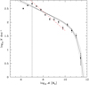 |
Fig. 27 SMF derived excluding the three cD galaxies NGC 1275, NGC 1272, and NGC 1265. The solid black and dotted black lines show the best-fit and ±1 σ confidence regions of the Schechter SMF parametrisation. The red dashed line, which is a reasonably good fit to the slope of the faint end of the distribution, has α = −1.35. The vertical grey dashed line shows the stellar mass limit used in the fit. The best-fit parameters are given in Table 4. |
8 Discussion
8.1 Compact sources
Studies of nearby clusters such as Virgo and Fornax indicate that, at the sensitivity of the Euclid observations, compact sources such as blue compact dwarfs (BCDs) and ultra compact dwarfs (UCDs) can be detected (Sandage et al. 1985; Boselli et al. 2016; Saifollahi et al. 2021). If reached, these particular populations of compact sources should thus be accounted for in the determination of the LF. The methods described above used to identify faint members of the Perseus cluster, and in particular those based on the positions of galaxies along several scaling relations, have been mainly defined to identify extended, LSB objects (e.g. Binggeli & Jerjen 1998). They might thus fail to recognise BCDs and UCDs, the former generally characterised by a relatively low luminosity but with a high surface brightness, which make them similar to background luminous star-forming systems, the latter by a point-like morphology similar to that of stars or globular clusters, which are generally poorly resolved in ground-based observations. To check whether these objects can be identified in the selection criteria mentioned in Sect. 4 we first derived the mean properties of approximately 40 BCDs in the Virgo cluster given in the Virgo Cluster Catalogue (VCC) of Binggeli et al. (1985). Using the full compilation of photometric data analysed in Boselli et al. (2014), we estimated that the mean B-band isophotal diameter of BCDs is D25.5(B) = 40″ ± 16″, while the H-band effective radius re(H) = ![$\[7^{\prime \prime}_\cdot4\]$](/articles/aa/full_html/2025/05/aa50808-24/aa50808-24-eq58.png) ±
± ![$\[4^{\prime \prime}_\cdot1\]$](/articles/aa/full_html/2025/05/aa50808-24/aa50808-24-eq59.png) . Scaled to the distance of the Perseus cluster (72 Mpc versus 16.5 Mpc for Virgo; Gavazzi & Boselli 1999; Mei et al. 2007; Cantiello et al. 2018) they are D25.5(b) = 10″ ± 4″ and re(H) =
. Scaled to the distance of the Perseus cluster (72 Mpc versus 16.5 Mpc for Virgo; Gavazzi & Boselli 1999; Mei et al. 2007; Cantiello et al. 2018) they are D25.5(b) = 10″ ± 4″ and re(H) = ![$\[1^{\prime \prime}_\cdot8\]$](/articles/aa/full_html/2025/05/aa50808-24/aa50808-24-eq60.png) ± 1″. BCDs are thus fully resolved in the Euclid data, even in the ring-filtered images which remove only star-like sources. They have B-, H-, and K-band absolute magnitudes MB ≥ −17 (Sandage et al. 1985) and MH ≥ −17.7 (Boselli et al. 2000), as well as MK ≥ −16.6 (Boselli et al. 1997), and have stellar masses ℳ ≲ 108 M⊙ (Boselli et al. 2014). They are, however, rare in rich environments where star formation is generally quenched due to the interaction of galaxies with their surroundings (e.g. Boselli & Gavazzi 2006). Those catalogued in the VCC and selected in the B band are 49/2096 (2.3%), and they are principally located at the periphery of the cluster. We checked the nature of all line emitters in the continuum-subtracted Hα narrow-band image to see whether we detected compact star-forming sources with morphological properties similar to those of local BCDs, but we did not detect any of them. BCDs are high-surface brightness objects with a very strong star-formation activity and are thus easily detectable in narrow-band imaging if present (Boselli et al. 2002, 2022a). Given that the Euclid observations concern only the inner ≲ 0.25 r200, that Perseus is a rich and massive cluster, and their very blue colour, we expect that the fraction of BCDs in the targeted region is significantly lower than the one observed in Virgo, as suggested by the analysis of the Hα data. We thus considered as negligible their possible contribution to our IE-band LF.
± 1″. BCDs are thus fully resolved in the Euclid data, even in the ring-filtered images which remove only star-like sources. They have B-, H-, and K-band absolute magnitudes MB ≥ −17 (Sandage et al. 1985) and MH ≥ −17.7 (Boselli et al. 2000), as well as MK ≥ −16.6 (Boselli et al. 1997), and have stellar masses ℳ ≲ 108 M⊙ (Boselli et al. 2014). They are, however, rare in rich environments where star formation is generally quenched due to the interaction of galaxies with their surroundings (e.g. Boselli & Gavazzi 2006). Those catalogued in the VCC and selected in the B band are 49/2096 (2.3%), and they are principally located at the periphery of the cluster. We checked the nature of all line emitters in the continuum-subtracted Hα narrow-band image to see whether we detected compact star-forming sources with morphological properties similar to those of local BCDs, but we did not detect any of them. BCDs are high-surface brightness objects with a very strong star-formation activity and are thus easily detectable in narrow-band imaging if present (Boselli et al. 2002, 2022a). Given that the Euclid observations concern only the inner ≲ 0.25 r200, that Perseus is a rich and massive cluster, and their very blue colour, we expect that the fraction of BCDs in the targeted region is significantly lower than the one observed in Virgo, as suggested by the analysis of the Hα data. We thus considered as negligible their possible contribution to our IE-band LF.
UCDs are much more compact than BCDs and for this reason are more difficult to be identified and distinguished from other point-like sources such as stars and globular clusters. Those identified in the Virgo cluster by Liu et al. (2020) have effective radii in the g and i bands of 10pc ≲ re(g, i) ≲ 100 pc, which at the distance of Perseus correspond to ![$\[0^{\prime \prime}_\cdot03\]$](/articles/aa/full_html/2025/05/aa50808-24/aa50808-24-eq61.png) ≲ re(g, i) ≲
≲ re(g, i) ≲ ![$\[0^{\prime \prime}_\cdot3\]$](/articles/aa/full_html/2025/05/aa50808-24/aa50808-24-eq62.png) , but most of them having re(g, i) ≲
, but most of them having re(g, i) ≲ ![$\[0^{\prime \prime}_\cdot1\]$](/articles/aa/full_html/2025/05/aa50808-24/aa50808-24-eq63.png) (see Penny et al. 2012). They are thus hardly resolved even at the excellent angular resolution of the Euclid VIS imaging data (FWHM =
(see Penny et al. 2012). They are thus hardly resolved even at the excellent angular resolution of the Euclid VIS imaging data (FWHM = ![$\[0^{\prime \prime}_\cdot16\]$](/articles/aa/full_html/2025/05/aa50808-24/aa50808-24-eq64.png) ). Their stellar mass is ℳ ≲ 107 M⊙, and their luminosity Mg ≥ −12 and MK ≥ −12.4 (Liu et al. 2020; Saifollahi et al. 2021). They are often associated with the central massive ellipticals (Liu et al. 2020; Saifollahi et al. 2021), and are thus potentially present in the Perseus field. The extraordinary quality of the Euclid data, however, allows the detection of these and other compact sources (globular clusters) associated with many massive galaxies. Their observed LF begins at IE ≃ 23 [M(IE) ~ −11.3] and steeply rises up to IE ≃ 25.5 or 26 [M(IE) ≃ −8.8 to −8.3], and drops below this. Being compact sources, we expect that the selection criteria mentioned in Sect. 4, and in particular the one used to discriminate stars from galaxies, have removed them from the sample of possible members. In any case, their contribution to the LF derived in this work, which is limited to galaxies with M(IE) > −11.3, is certainly negligible.
). Their stellar mass is ℳ ≲ 107 M⊙, and their luminosity Mg ≥ −12 and MK ≥ −12.4 (Liu et al. 2020; Saifollahi et al. 2021). They are often associated with the central massive ellipticals (Liu et al. 2020; Saifollahi et al. 2021), and are thus potentially present in the Perseus field. The extraordinary quality of the Euclid data, however, allows the detection of these and other compact sources (globular clusters) associated with many massive galaxies. Their observed LF begins at IE ≃ 23 [M(IE) ~ −11.3] and steeply rises up to IE ≃ 25.5 or 26 [M(IE) ≃ −8.8 to −8.3], and drops below this. Being compact sources, we expect that the selection criteria mentioned in Sect. 4, and in particular the one used to discriminate stars from galaxies, have removed them from the sample of possible members. In any case, their contribution to the LF derived in this work, which is limited to galaxies with M(IE) > −11.3, is certainly negligible.
8.2 Robustness of the derived parameters
The three cD galaxies in the core of the cluster (NGC 1275, NGC 1272, and NGC 1265) introduce a discontinuity in the LF that cannot be traced by our simple parametric function given in Eq. (2). We thus fit the data including all galaxies with an absolute magnitude M(IE) ≤ −11.33, or excluding either NGC 1275, or the three brightest objects NGC 1275, NGC 1272, and NGC 1265. The best fit to the data derived using these three different samples are given in Table 3. Figure 28 shows the probability distribution functions of the output parameters derived when the three cD galaxies are excluded.
As expected, the output parameters of the Gaussian function strongly depend on the adopted sample, that is, on the inclusion or exclusion of the brightest cD galaxies. This is due to the fact that the number of bright objects is very limited, thus any output parameter in this magnitude regime is statistically uncertain. More interesting, in the framework of galaxy formation and evolution, is the faint end of the LF. The faint end slope of the LF, αS, is robustly determined, as depicted in Fig. 28, and around αS = −1.2 to −1.3. This is significantly flatter than the slope of the dark matter halo mass function predicted by cosmological simulations (α ≃ −2, e.g. Somerville & Davé 2015). This is also the case if the fit is limited to the steep rise of the distribution [M(IE) ≲ −15], where αS ≃ −1.5, and drops to αS ≃ −1.1 in the −15 ≲ M(IE) ≲ −11.3 magnitude range. Any possible missed satellite, if it exists, must have a surface brightness at re (μIE,e) ≳ 29 mag arcsec−2.
8.3 Comparison with other works
The IE-band LF of the Perseus cluster measured within R ≲ 0.25 r200 is compared to those derived in other bands in Fig. 26. The faint-end slope of the fitted function is compared to those derived in these other works at different wavelengths in Fig. 29. These have been determined in the K band using WISE 2.4-μm data by Meusinger et al. (2020) and concern the inner R ~ r200, and in the r band by Aguerri et al. (2020, R ~ 1.4 r200). The IE-band LF is also compared with that of Penny & Conselice (2008) measured in the B band for a limited number of dwarfs in the very inner regions of the cluster. To compare LF derived in different photometric bands, we cross-matched the Euclid catalogue with those used in previous studies. We estimated the mean colour in the different bands, which we then used as a systematic correction on the X-axis. Since the Y-axis normalisation depends on the sampled volume, which varies across these studies, we arbitrarily chose the normalisation on this axis to match the distribution observed in the IE band.
The IE-band LF derived in this work is significantly deeper than those of Meusinger et al. (2020) and Aguerri et al. (2020), which are both limited to the bright end, M(IE) ≃ −18.3 and M(IE) ≃ −16.2, respectively, when these limiting magnitudes are derived using the mean colour of common galaxies in the different bands. It is also deeper than that of Penny & Conselice (2008, M(IE) ≃ −13.9), although that does not sample the bright end given the very limited sky region covered during the observations (173 arcmin2).
For a fair comparison, three things should be remembered. Firstly, the IE-band LF measured in this work concerns only the inner R ≲ 0.25 r200 which, for the well known morphology-segregation effect (Dressler 1980a; Whitmore et al. 1993), is highly dominated by early-type systems. Indeed, the number of star-forming galaxies is limited to a handful of objects, as depicted in the colour–magnitude diagram shown in Fig. 21. Secondly, the overall shape of the LF is known to change at different distances from the cluster centre (e.g. Beijersbergen et al. 2002; Popesso et al. 2006; de Filippis et al. 2011). Finally, the shape also changes as a function of the photometric band (e.g. Andreon & Cuillandre 2002; Popesso et al. 2005; Boselli et al. 2016).
The IE-band LF measured in this paper agrees with the decrease observed at M(IE) ≃ −19 by Meusinger et al. (2020) and Aguerri et al. (2020) when limited to the early-type galaxy population. This decrease is due to the presence of the dip, which corresponds to the relative decrease of objects at IE ~ 15 in the scaling relations shown in Fig. 25 (see also Figure 12 of Marleau et al. 2025). The faint end of the IE-band LF is comparable to the one observed in the B band by Penny & Conselice (2008) in the same magnitude range.
The IE-band LF of Perseus can also be compared to those derived for other nearby clusters of galaxies. Figure 26 shows the comparison with the i-band LF of composite SDSS clusters measured within R < 0.5 h−1 Mpc by Popesso et al. (2005). It shows a discontinuity at M(IE) ≃ −19, where the IE-band LF of Perseus has a dip, and is significantly steeper at fainter luminosities (α = −2.17; see also Fig. 29). The presence of the dip with properties similar to the one presented here has been observed in other very massive nearby clusters, such as Coma (Biviano et al. 1995; Lobo et al. 1997; de Propris et al. 1998; Adami et al. 2007; Milne et al. 2007) and Abell 85 (Durret et al. 1999). The slope of the LF in the −19 ≲ M(IE) ≲ −14 absolute magnitude range is α ≃ −1.5, and is significantly flatter than the one derived by Popesso et al. (2005, α ≃ −2.17). However, this difference should be considered with caution for several reasons. First of all, this luminosity range is generally lacking spectroscopic data; thus cluster membership is often derived using statistical arguments, such as a statistical subtraction of the background galaxy counts, as done in Popesso et al. (2005). This technique is obviously very sensitive to sampling variance, since in this luminosity regime the number of background galaxies largely exceeds that of cluster members. For the region analysed in this work, for instance, the number of galaxies detected by SourceExtractor with IE < 23.6 is about 33 000, most of which have faint luminosities (see Sect. 4), with only 1220 finally being identified as cluster members. As a consequence, the statistical subtraction of the background galaxy counts introduces large uncertainties at the faint end, as suggested by the very discrepant results obtained even on the same cluster when different techniques are used (see Fig. 29). In the Coma cluster, by far the most studied local massive cluster of galaxies, the results obtained so far give slopes ranging from α = −1.0 to α = −2.0 (see table 1 in Milne et al. 2007; Yamanoi et al. 2012), suggesting that the faint end slope of the LF is still poorly constrained whenever the identification of cluster members suffers from large uncertainties. This is also the case in other nearby clusters where different values of α are often derived when using different techniques to account for the background contamination (e.g. Boué et al. 2008). We will be able to test this statistical correction and compare the results to those found in this work once a robust estimate of the galaxy number counts is measured thanks to the Euclid mission.
A particular case is the Virgo cluster. Located at only 16.5 Mpc (Gavazzi & Boselli 1999; Mei et al. 2007; Cantiello et al. 2018), this is the closest cluster of galaxies and for this reason it has been the target of several multifrequency surveys. Thanks to its proximity, deep ground-based imaging surveys can easily sample the dwarf galaxy regime over a luminosity range comparable to the one reached by Euclid in Perseus. NGVS (Ferrarese et al. 2012) managed to detect and identify cluster members down to a stellar mass limit of ℳ ≃ 106 M⊙. The typical angular resolution of these data, ![$\[0^{\prime \prime}_\cdot6\]$](/articles/aa/full_html/2025/05/aa50808-24/aa50808-24-eq65.png) in the i band (49 pc), is comparable to the physical scales probed by VIS in the IE band at the distance of Perseus (
in the i band (49 pc), is comparable to the physical scales probed by VIS in the IE band at the distance of Perseus (![$\[0^{\prime \prime}_\cdot16\]$](/articles/aa/full_html/2025/05/aa50808-24/aa50808-24-eq66.png) , 56 pc, see Sect. 3.1). Ferrarese et al. (2016) derived the i-band LF of the cluster within R ≃ 0.2 r200 down to Mi ≃ −10, where the 336 cluster members have been identified with criteria very similar to those used in this work. The two sets of data can thus be directly compared. The bright part of i-band Virgo cluster LF is poorly constrained because of the very limited number of massive objects; it is thus impossible to see whether a dip is present also in this cluster. The faint end, however, is well represented by a Schechter function of slope α = −1.35, a value slightly steeper than the one found for Perseus (−1.30 ≲ α ≲ −1.20). This difference is not surprising given that Perseus is a very massive spiral-poor relaxed cluster (M200 = 1.2 × 10¹⁵ M⊙), while Virgo is a spiral-rich, intermediate mass unrelaxed system (M200 = 1–4 × 10¹⁴ M⊙, Ferrarese et al. 2012; Boselli et al. 2022b). A flattening of the B-band LF measured in selected regions out to R ≃ 1 r200 in the magnitude range −14 ≲ MB ≲ −11 has been claimed by Trentham & Hodgkin (2002, α = −1.3 to −1.0) with shallower INT data, and only partly confirmed by the deeper NGVS data in the inner region (α = −1.39 for −17.4 ≲ Mg ≲ −14.4 versus α = −1.26 for −14.4 ≲ Mg ≲ −9.13, Ferrarese et al. 2016).
, 56 pc, see Sect. 3.1). Ferrarese et al. (2016) derived the i-band LF of the cluster within R ≃ 0.2 r200 down to Mi ≃ −10, where the 336 cluster members have been identified with criteria very similar to those used in this work. The two sets of data can thus be directly compared. The bright part of i-band Virgo cluster LF is poorly constrained because of the very limited number of massive objects; it is thus impossible to see whether a dip is present also in this cluster. The faint end, however, is well represented by a Schechter function of slope α = −1.35, a value slightly steeper than the one found for Perseus (−1.30 ≲ α ≲ −1.20). This difference is not surprising given that Perseus is a very massive spiral-poor relaxed cluster (M200 = 1.2 × 10¹⁵ M⊙), while Virgo is a spiral-rich, intermediate mass unrelaxed system (M200 = 1–4 × 10¹⁴ M⊙, Ferrarese et al. 2012; Boselli et al. 2022b). A flattening of the B-band LF measured in selected regions out to R ≃ 1 r200 in the magnitude range −14 ≲ MB ≲ −11 has been claimed by Trentham & Hodgkin (2002, α = −1.3 to −1.0) with shallower INT data, and only partly confirmed by the deeper NGVS data in the inner region (α = −1.39 for −17.4 ≲ Mg ≲ −14.4 versus α = −1.26 for −14.4 ≲ Mg ≲ −9.13, Ferrarese et al. 2016).
The results obtained in this work are consistent with those available in the literature for Virgo, and extend those derived for other very massive clusters such as Perseus to a luminosity range never explored before. They provide a unique sample for comparison with the prediction of cosmological simulations to constrain galaxy evolution in a very rich environment.
Finally, we compare the observed LF to that predicted for cluster galaxies using the Cluster-EAGLE cosmological simulations in the SDSS i band (Negri et al. 2022). The two LFs are fairly different: the cosmological simulations do not show an obvious dip at M(IE) ≃ −19, but just a flattening of the curve, although they have a faint-end slope in the sampled magnitude range [M(IE) < −15] close (α = −1.3) to the observed one. The LF of Negri et al. (2022) has been derived combining 30 clusters of mass 1014 ≲ M200/M⊙ ≲ 1015.4 with galaxies located within R = r200. The difference with the observed one might partially be due to the fact that in Perseus we are sampling only the very innermost regions (R ≲ 0.25 r200) and that Perseus is a very massive cluster, where a dip at intermediate luminosity is generally observed.
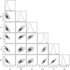 |
Fig. 28 Probability distribution function of the output parameters of the fit of the luminosity function for a Schechter + Gauss parametric function when the galaxies NGC 1275, NGC 1272, and NGC 1265 are excluded. |
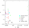 |
Fig. 29 Faint-end slope αS of the LF derived in this work [M(IE) ≤ −12; big filled cyan circle] compared to the values of the analogous Schechter parameters α available in the literature in different photometric bands for the Perseus cluster (green circles, references given in the text), for the Coma cluster (red boxes, taken from the compilation of Milne et al. 2007), the Virgo cluster (blue triangles, from the compilation of Ferrarese et al. 2016), and for the composite LF of clusters of Popesso et al. (2005, black hexagons, double Schechter functions, measured using two different background subtraction techniques within 0.5 Mpc). Empty symbols are for LF of the whole cluster, and filled symbols for the core region, as in the Euclid field. |
8.4 Implications of the results in an evolutionary picture
The field galaxy LF and SMF are generally considered to be composed of two different components, one for the quiescent population and one for the star-forming systems, dominant in low-density regimes (Bell et al. 2003; Baldry et al. 2012; Muzzin et al. 2013). They can both be represented by two functions. The former, generally characterised by a Gaussian or a Schechter function declining at faint luminosities (α > −1), is dominated in the high-luminosity, high-mass regime. The latter, mainly fitted with a Schechter function, is dominant at the faint end. In the cluster environment the relative weight of the two populations is significantly changed, in particular at the faint end where the dominant population consists of dwarf ellipticals (e.g. Sandage et al. 1985). Given the tight positive relation between the fraction of slow/fast rotators with stellar mass (Cappellari 2016) observed also in clusters such as Virgo (Boselli et al. 2014), it is likely that the Gaussian part of the luminosity and mass functions are dominated by massive ellipticals formed during major merging events, and those of lower luminosities/stellar masses by gentler mechanisms.
The steep rise of the dwarf elliptical galaxy population in the luminosity range −19 ≲ M(IE) ≲ −14 observed here and in other nearby clusters (e.g. Sandage et al. 1985) can be explained if the galaxies infalling into the cluster since its formation, which are preferentially star-forming objects, are quenched after their interaction with the hostile surrounding environment (e.g. Boselli & Gavazzi 2014). We recall that the field LF, when measured including the dominant LSB population, has a slope in the visible bands close to α = −1.5 (Blanton et al. 2005b). A simple fading of the star-formation activity, which might follow ram-pressure-stripping events (e.g. Boselli et al. 2022b), can transform blue galaxies into red systems (e.g. Gavazzi et al. 2010) without affecting their structural (e.g. Boselli et al. 2008b,a) and kinematic properties (e.g. Toloba et al. 2011, 2015), and more important the shape of the luminosity and mass functions. This evolutionary picture is consistent with the observed variation of the slope of the LF of the Virgo cluster derived using tracers sensitive to the youngest stellar populations (Hα, UV, Boselli et al. 2016, 2023) or to older populations (visible bands, Sandage et al. 1985; Ferrarese et al. 2016). It is also consistent with the observed increase of the fraction of red/blue galaxies with decreasing redshift at the faint end of the LF in clusters of galaxies (De Lucia et al. 2007, 2009; Stott et al. 2007, 2009; Gilbank et al. 2008; Boselli & Gavazzi 2014).
The flattening at lower luminosities should still be confirmed with more accurate spectroscopic observations. If borne out, lowest-mass objects gravitationally perturbed during their flyby encounters with other cluster members (galaxy harassment, Moore et al. 1996; Mastropietro et al. 2005a) might explain this flattening. In the most extreme cases a large fraction of the mass is removed during the interaction, leaving just the galaxy nucleus (Bekki et al. 2003; Drinkwater et al. 2003; Goerdt et al. 2008; Pfeffer & Baumgardt 2013). This mechanism, which has been often proposed to explain the formation of UCDs, might reduce the number of objects in this luminosity/mass regime, flattening the observed distribution. Interestingly, Kluge et al. (2025) have shown a significant contribution of dwarf galaxies to the intracluster globular cluster LF. These dwarf galaxies would be entirely disrupted to form the ICL so this could partly explain the observed difference between the steep faint-end slope of the dark matter halo distribution predicted by simulations with the flatter slope observed in the LF and SMF. This speculative interpretation should be tested by comparison with hydrodynamic cosmological simulations once they reach this very low-mass regime with sufficient statistics.
8.5 Perspectives
The analysis and results presented in this work demonstrate the extraordinary capabilities of Euclid in the study of galaxy evolution in rich environments. Although not reaching the spectacular angular resolution of Hubble Space Telescope (HST), Euclid will provide a homogeneous set of optical (and NIR) images with a typical FWHM ~ ![$\[0^{\prime \prime}_\cdot16\]$](/articles/aa/full_html/2025/05/aa50808-24/aa50808-24-eq67.png) (~
(~![$\[0^{\prime \prime}_\cdot49\]$](/articles/aa/full_html/2025/05/aa50808-24/aa50808-24-eq68.png) ) over more than 14 000 deg2. This resolution will be crucial for the identification of galaxies belonging to different local environments, from massive clusters such as Perseus down to groups and filaments, hundreds of which will be covered during the mission. Furthermore, the extraordinary quality of the images in terms of sensitivity to LSB regions will be crucial to studying different characteristic features associated with galaxies in rich environments, such as tails, filaments, shells of tidally perturbed objects (Duc et al. 2015), or the intracluster light present in the central regions of massive clusters (Kluge et al. 2025). These particular stellar features are formed only during gravitational perturbations that are able to displace the stellar component, while not in hydrodynamic interactions affecting only the gas (e.g. Boselli et al. 2022b). The Euclid observations will thus be of prime importance for the identification of the dominant perturbing mechanism in different environments, from filaments and groups, to massive clusters. It will also be extremely important to identify UDGs, a population seen in nearby clusters as well as in the field (Marleau et al. 2024; Koda et al. 2015; Mihos et al. 2015; van Dokkum et al. 2015b; Zöller et al. 2024), whose origin is still under debate (Di Cintio et al. 2017; Carleton et al. 2019; Tremmel et al. 2020; Junais et al. 2022).
) over more than 14 000 deg2. This resolution will be crucial for the identification of galaxies belonging to different local environments, from massive clusters such as Perseus down to groups and filaments, hundreds of which will be covered during the mission. Furthermore, the extraordinary quality of the images in terms of sensitivity to LSB regions will be crucial to studying different characteristic features associated with galaxies in rich environments, such as tails, filaments, shells of tidally perturbed objects (Duc et al. 2015), or the intracluster light present in the central regions of massive clusters (Kluge et al. 2025). These particular stellar features are formed only during gravitational perturbations that are able to displace the stellar component, while not in hydrodynamic interactions affecting only the gas (e.g. Boselli et al. 2022b). The Euclid observations will thus be of prime importance for the identification of the dominant perturbing mechanism in different environments, from filaments and groups, to massive clusters. It will also be extremely important to identify UDGs, a population seen in nearby clusters as well as in the field (Marleau et al. 2024; Koda et al. 2015; Mihos et al. 2015; van Dokkum et al. 2015b; Zöller et al. 2024), whose origin is still under debate (Di Cintio et al. 2017; Carleton et al. 2019; Tremmel et al. 2020; Junais et al. 2022).
9 Conclusions
The Euclid ERO programme gathered deep optical and NIR imaging data of the inner regions (R ≤ 0.25 r200) of the nearby Perseus cluster. We used this unique set of imaging data, which reached a point-source depth of IE = 27.3 and surface brightnesses μIE = 30.1 mag arcsec−2, to measure the LF and SMF of this cluster. We identified cluster members out of the roughly half-million detected sources using a combination of photometric redshifts, scaling relations, cross-matches with catalogues available in the literature, and visual inspection of the images. We identified 1220 cluster members. Using the observed distribution of their structural properties (total magnitude, surface brightness, extension, Sérsic parameter, and inclination), we accurately measured the completeness function of the sample, which reaches about 50% at M(IE) = −11.33. We derived the IE-band LF of the inner region of the cluster and fit it using a parametric Schechter plus Gaussian function, which reproduces the observed distribution well, particularly whenever the three brightest cD galaxies (NGC 1275, NGC 1272, and NGC 1265) are excluded. The fitted function, which is significantly deeper than those derived so far using ground-based data, has a dip at M(IE) ≃ −19 and a faint-end slope αS ≃ −1.2 to −1.3. We used the unique set of multifrequency data in hand, which also include deep unpublished ugriz and narrow-band Hα imaging data gathered at the CFHT, to measure the stellar mass of all the cluster members and thus derive the SMF of the cluster. The SMF can be represented by a Schechter function with a faint-end slope αS ≃ −1.2 to −1.35.
Despite the exceptional sensitivity of Euclid to LSB objects, which are expected to dominate at faint luminosities, the observed faint-end slope of the LF and SMF of Perseus are significantly flatter than those predicted for the dark matter halo distribution by cosmological simulations. The unique set of data that the Euclid mission will soon provide will be crucial to extending this analysis to a much larger sample of local galaxies in different environments, from the field to groups and rich clusters. These data will offer new stringent constraints to cosmological simulations on galaxy evolution and thus provide a unique opportunity to understand the processes that shape the LF and SMF in different environments.
Data availability
Full Tables C.3–C.9 are available at the CDS via anonymous ftp to cdsarc.cds.unistra.fr (130.79.128.5) or via https://cdsarc.cds.unistra.fr/viz-bin/cat/J/A+A/697/A11
Acknowledgements
This work has made use of the Early Release Observations (ERO) data from the Euclid mission of the European Space Agency (ESA), 2024, https://doi.org/10.57780/esa-qmocze3. The Euclid Consortium acknowledges the European Space Agency and a number of agencies and institutes that have supported the development of Euclid, in particular the Agenzia Spaziale Italiana, the Austrian Forschungsförderungsgesellschaft funded through BMK, the Belgian Science Policy, the Canadian Euclid Consortium, the Deutsches Zentrum für Luft- und Raumfahrt, the DTU Space and the Niels Bohr Institute in Denmark, the French Centre National d’Etudes Spatiales, the Fundação para a Ciência e a Tecnologia, the Hungarian Academy of Sciences, the Ministerio de Ciencia, Innovación y Universidades, the National Aeronautics and Space Administration, the National Astronomical Observatory of Japan, the Netherlandse Onderzoekschool Voor Astronomie, the Norwegian Space Agency, the Research Council of Finland, the Romanian Space Agency, the State Secretariat for Education, Research, and Innovation (SERI) at the Swiss Space Office (SSO), and the United Kingdom Space Agency. A complete and detailed list is available on the Euclid web site (http://www.euclid-ec.org). Based on observations obtained with MegaPrime/MegaCam, a joint project of CFHT and CEA/DAPNIA, at the Canada-France-Hawaii Telescope (CFHT) which is operated by the National Research Council (NRC) of Canada, the Institut National des Science de l’Univers of the Centre National de la Recherche Scientifique (CNRS) of France, and the University of Hawaii. The observations at the Canada-France-Hawaii Telescope were performed with care and respect from the summit of Maunakea which is a significant cultural and historic site. This work presents results from the European Space Agency (ESA) space mission Gaia. Gaia data are being processed by the Gaia Data Processing and Analysis Consortium (DPAC). Funding for the DPAC is provided by national institutions, in particular the institutions participating in the Gaia MultiLateral Agreement (MLA). Funding for the Sloan Digital Sky Survey V has been provided by the Alfred P. Sloan Foundation, the Heising-Simons Foundation, the National Science Foundation, and the Participating Institutions. SDSS acknowledges support and resources from the Center for High-Performance Computing at the University of Utah. SDSS telescopes are located at Apache Point Observatory, funded by the Astrophysical Research Consortium and operated by New Mexico State University, and at Las Campanas Observatory, operated by the Carnegie Institution for Science. The SDSS web site is www.sdss.org. SDSS is managed by the Astrophysical Research Consortium for the Participating Institutions of the SDSS Collaboration, including Caltech, The Carnegie Institution for Science, Chilean National Time Allocation Committee (CNTAC) ratified researchers, The Flatiron Institute, the Gotham Participation Group, Harvard University, Heidelberg University, The Johns Hopkins University, L’Ecole polytechnique fédérale de Lausanne (EPFL), Leibniz-Institut für Astrophysik Potsdam (AIP), Max-Planck-Institut für Astronomie (MPIA Heidelberg), Max-Planck-Institut für Extraterrestrische Physik (MPE), Nanjing University, National Astronomical Observatories of China (NAOC), New Mexico State University, The Ohio State University, Pennsylvania State University, Smithsonian Astrophysical Observatory, Space Telescope Science Institute (STScI), the Stellar Astrophysics Participation Group, Universidad Nacional Autónoma de México, University of Arizona, University of Colorado Boulder, University of Illinois at Urbana-Champaign, University of Toronto, University of Utah, University of Virginia, Yale University, and Yunnan University. CS acknowledges the support of the Natural Sciences and Engineering Research Council of Canada (NSERC). Cette recherche a été financée par le Conseil de recherches en sciences naturelles et en génie du Canada (CRSNG). CS also acknowledges support from the Canadian Institute for Theoretical Astrophysics (CITA) National Fellowship program. FB acknowledges support from the project PID2020-116188GA-I00, funded by MICIU/AEI /10.13039/501100011033. LQ acknowledges funding from CNES postdoctoral fellowship program.
Appendix A Overview of the science programme
The extraordinary data quality and richness of this ERO Perseus cluster programme opens the door to other exciting analyses. In the following subsections, we briefly present soon-to-be published research activities by the ERO Perseus science team beyond the primary focus of this paper.
Appendix A.1 Dwarf galaxies
Dwarf galaxies are the oldest and most numerous galaxy type in the Universe (Binggeli et al. 1990; Ferguson & Binggeli 1994), yet the driving mechanism(s) in their evolution and the transformation into the different types we see today remains elusive. The two main types are the dwarf irregular (dI) galaxies and the dwarf elliptical/spheroidal (dE/dSph) galaxies, but many other sub-classes make up this population of galaxies, such as UCDs and UDGs. The defining distinction between dwarf and giant galaxies is that dwarfs are extremely faint, with magnitudes fainter than −18 in the V band (Aaronson et al. 1985), although this magnitude limit varies greatly in the literature (see, for example, Hodge 1971). They are also defined by their typically low stellar masses (≤ 109 M⊙, Bullock & Boylan-Kolchin 2017) and small physical sizes, with sizes ranging from a few hundred parsecs to a few kiloparsecs. Dwarf galaxies often host globular clusters (GCs), which can be used to probe the underlying mechanisms driving galaxy assembly, the dynamics of stellar populations, and the influence of environment on star-formation processes.
In Marleau et al. (2025), we conduct a comprehensive census of the dwarf galaxies, their nuclei, and their globular cluster populations in the Perseus ERO programme. Our study maps their spatial distribution and visual morphologies, while also extracting their photometric and structural properties. Our analysis reveals a total of 1100 dwarf galaxy candidates, 630 of which are found to be new discoveries. The morphological mix consists of 96% dE, 53% nucleated, 26% GC-rich, and 6% with disturbed morphology. We classify a relatively high fraction of galaxies, 9%, as UDGs. The majority of the dwarf candidates follow the scaling relations of dwarf galaxies in the literature. However, our dwarf sample significantly extends the known scaling relation towards diffuse galaxies. In agreement with studies of nucleated populations, we find fewer nuclei in faint, small, and high-ellipticity dwarfs, with flatter surface brightness profiles. Globally, the GC specific frequency, S N, of the Perseus dwarf candidates is intermediate between those measured in the Virgo and Coma clusters. While the dwarf candidates with the largest GC counts are found throughout the Euclid FoV, the dwarfs located around the east-west strip, where most of the brightest cluster members are found, exhibit larger S N, on average.
Appendix A.2 Asymmetries in dwarf galaxies for studying environmental processes
Dwarf galaxies are excellent tracers of the effects of environment, due to their LSB signature. We analyse the morphology of dwarf galaxies in Perseus to study the role of the environment in this massive cluster, where strong gravitational forces shape the evolution of its galaxies. We concentrate on the asymmetries of early-type dwarfs (dE and dSph), which are a solid indicator of tidal forces (see Penny et al. 2011). We conducted such an analysis for the 564 dwarfs catalogued in the Fornax Deep Survey (Venhola et al. 2018). Penny et al. (2011) found strong asymmetries in 11 galaxies in HST data of the outer parts of Perseus. With the Euclid data on the Perseus cluster, strong of 1100 dwarf galaxies, we now have a 100-fold increase in the number of dwarf galaxies available, permitting a comprehensive analysis of their morphological evolution within the cluster.
Appendix A.3 Environmental dependence of the nucleation fraction in dwarf galaxies
nuclear star clusters (NSCs) are compact stellar systems with sizes (half-light radii) of 1–50 pc and stellar masses spanning several decades, from as low as 104 M⊙ to as high as 108 M⊙. This makes them, on average, larger and more massive than a typical GC, and their central stellar surface densities can be even more extreme. Sitting at the bottom of their host galaxy’s potential well, NSC stellar populations and dynamics encode a record of the formation and evolution of galactic inner regions (see Neumayer et al. 2020, and references therein) and inform us about the efficiency of high-pressure star formation at early times.
NSCs are found in galaxies spanning a wide range of masses, morphological types and environments, and nucleation seems to be a complex function of all these parameters. Recent studies in the nearby Universe have cemented the role of galaxy mass/luminosity as the main driver of NSC occurrence (Sánchez-Janssen et al. 2019). Remarkably, they have also uncovered an unambiguous secondary dependence on the environment at low galaxy masses [6 < log10(ℳ/M⊙) < 9], whereby more massive haloes feature higher nucleation fractions than lower density environments (Hoyer et al. 2021; Poulain et al. 2021; Zanatta et al. 2021, 2024). With a virial mass M200 ~ 1015 M⊙ Perseus is an ideal laboratory to study nucleation at extreme environmental densities, with over a thousand dwarfs already identified as candidate cluster satellites within the Euclid footprint (Marleau et al. 2025). We will take advantage of Euclid’s exquisite sensitivity for both extended and compact sources to carry out a comprehensive study of the phenomenon of nucleation down to the luminosity regime of the ‘classical’ Galactic satellites as well as to provide a thorough comparison with other relevant environments in the nearby Universe.
Appendix A.4 Globular clusters of dwarf galaxies
In this project, we use Euclid ERO data on the Perseus galaxy cluster and identify GCs around dwarf galaxies in this cluster. Given the observations of a number of GC-rich dwarf galaxies in nearby galaxy clusters (Amorisco et al. 2018; Prole et al. 2019; Lim et al. 2020; Saifollahi et al. 2022) and galaxy groups (Müller et al. 2021; Carlsten et al. 2022), the GC content of dwarf galaxies has become a topic of interest in the past few years. The GC-rich dwarfs host a few times more GCs compared to the general population of dwarf galaxies of the same stellar mass. It appears that the high-density environments within galaxy clusters, environments similar to the environment of the Perseus cluster, play a role in the formation of GC-rich dwarf galaxies. However, until now, most of the observations have focused on a sub-class of dwarf galaxies with large size and very low surface brightness, known as UDGs (van Dokkum et al. 2015a). In the meantime, the GC properties of the general population of dwarf galaxies have not been studied in detail, which potentially can lead to inconsistencies in interpretations of GC observations of UDGs.
However, now, with the ERO data of the Perseus cluster, we are able to have a uniform analysis and in-depth study of the GC properties of more than 1000 dwarf galaxies, including several UDGs. Given the spatial resolution, as well as the depth of the Euclid IE-band image of this ERO programme, we are able to identify GCs brighter than the turn-over magnitude of the GC luminosity function (GCLF) at the distance of the Perseus galaxy cluster (Kluge et al. 2025; Marleau et al. 2025). For the GCs, the combination of IE with the three Euclid NISP bands, YE, JE, and HE, help further clean the sample of GC candidates from possible contaminants (Saifollahi et al. 2025, Euclid Collaboration: Voggel et al. in prep.). As a result of our search for GCs, we produce catalogues of GC candidates for each dwarf galaxy identified within the ERO data. Then, using these catalogues, we examine the properties of GCs of dwarf galaxies in the Perseus cluster for a wide range of galaxy luminosities and sizes, and study the galaxy-GC scaling relations. Furthermore, given the correlation between GC numbers and galaxy halo mass (Spitler & Forbes 2009; Harris et al. 2013), we convert the estimated GC numbers to dwarf halo mass and further investigate their stellar-to-halo mass ratios.
Appendix A.5 Measuring distances to early-type and dwarf galaxies using surface brightness fluctuations
The surface brightness fluctuation (SBF) method is a robust technique for determining distances to early-type galaxies out to about 200 Mpc (and beyond, with JWST data, see Cantiello & Blakeslee 2023, and references therein). By measuring intrinsic variance in surface brightness distribution, it estimates distance with up to 5% accuracy for individual targets (Mei et al. 2007; Blakeslee et al. 2021; Jensen et al. 2021). The SBF signal arises from the stochastic stellar counts and luminosities in the host stellar population and corresponds to a quantity closely related to the luminosity-weighted mean brightness of the stars within the target galaxy (Tonry & Schneider 1988; Tonry et al. 1990).
To derive the distances from SBF, accurate knowledge of fluctuations of magnitude (![$\[\bar{m}\]$](/articles/aa/full_html/2025/05/aa50808-24/aa50808-24-eq69.png) ) and absolute magnitude (
) and absolute magnitude (![$\[\bar{M}\]$](/articles/aa/full_html/2025/05/aa50808-24/aa50808-24-eq70.png) ) in the same passband is crucial. Typically,
) in the same passband is crucial. Typically, ![$\[\bar{M}\]$](/articles/aa/full_html/2025/05/aa50808-24/aa50808-24-eq71.png) is calibrated in a two-step procedure: first using galaxies with known distances to establish the zero point, and then examining the dependence of
is calibrated in a two-step procedure: first using galaxies with known distances to establish the zero point, and then examining the dependence of ![$\[\bar{M}\]$](/articles/aa/full_html/2025/05/aa50808-24/aa50808-24-eq72.png) on stellar population properties (see e.g. Tonry et al. 2001; Cantiello et al. 2018). This is often done using galaxies at a common distance (e.g. in groups or clusters) and colour measurements to standardise the stellar population dependence of
on stellar population properties (see e.g. Tonry et al. 2001; Cantiello et al. 2018). This is often done using galaxies at a common distance (e.g. in groups or clusters) and colour measurements to standardise the stellar population dependence of ![$\[\bar{M}\]$](/articles/aa/full_html/2025/05/aa50808-24/aa50808-24-eq73.png) .
.
Euclid’s high-resolution imaging, depth, and wide sky survey area offer potential for precise SBF measurements for thousands of galaxies in the local Universe. This makes the Perseus ERO programme invaluable for testing and calibrating SBF measurement procedures using Euclid’s specific dataset.
SBF magnitudes (and colours) offer insights into unresolved stellar populations in targeted galaxies (Jensen et al. 2015). Despite lower angular resolution in NIR observations, NISP instrument will provide ample data for NIR SBF magnitude calibration, particularly beneficial for elliptical galaxies where red-giant-branch stars dominate NIR flux. Contemporary VIS and NISP fluctuation amplitudes aid in understanding potential sources of scatter, such as the impact of intermediate-age asymptotic giant branch stars on NIR SBF (Cantiello et al. 2003; Raimondo 2009).
The Perseus cluster, at 72 Mpc, is an ideal environment for SBF measurements. Its minimal depth effects enable precise characterisation of the SBF amplitude relative to galaxy colour, available from Euclid’s VIS and NISP imaging. We aim to conduct SBF measurements on all Perseus cluster galaxies with smooth morphology using VIS and NISP imaging data. Challenges include standardising ![$\[\bar{M}\]$](/articles/aa/full_html/2025/05/aa50808-24/aa50808-24-eq74.png) in the IE band (due to its wide wavelength range), and addressing undersampling of the PSF in NISP data. Preliminary tests are currently underway.
in the IE band (due to its wide wavelength range), and addressing undersampling of the PSF in NISP data. Preliminary tests are currently underway.
Appendix A.6 Spatially resolved stellar populations
The deep images and highly resolved, precise photometry obtained in the optical and NIR by Euclid on the Perseus cluster enable the mapping of spatially resolved stellar mass density of galaxies in the field via resolved SED fitting. Combining these datasets with UV and optical imaging from GALEX (Morrissey et al. 2007) and CFHT offers sufficient constraints on other important properties, including stellar age, metallicity, and even star-formation history. By deriving spatially resolved maps of stellar mass and other properties of the stellar populations, we can delve deeper into the understanding of the assembly of galaxy mass within the cluster, disentangling the roles of endogenous galaxy processes, environmental influences, and galaxy mergers. The mass profiles derived will be the benchmark for future kinematic and dynamical follow-up studies and high-resolution H I and H2 gas maps and masses to constrain the interplay of the small-scale physics of gas and star formation with galaxy-scale properties.
We used the piXedfit (Abdurro’uf et al. 2021, 2022a; Abdurro’uf, et al. 2022b) pipeline to perform spatially resolved SED fitting on the combined data from Euclid and CFHT. This code has been rigorously tested on galaxies simulated by the TNG collaboration (Abdurro’uf et al., in prep.). Leveraging synthetic spectral models (e.g. Bruzual & Charlot 2003), we determined the best-fitting template and its characteristic stellar population parameters for each pixel, thereby constructing stellar population maps for the target galaxies extending to their outer galactic regions. For NGC 1268, in Fig. A.1 we show the 2D maps of the fluxes in each band and mass density map obtained after SED fitting.
Appendix A.7 The mysterious origin of NGC 1277
NGC 1277 is the most extreme case of a relic galaxy, that is, a local counterpart of the massive ultra-compact galaxy population also known as ‘red nuggets’ common at z > 2 (Ferré-Mateu et al. 2017; Spiniello et al. 2024). How this object remains similar to those in the primeval Universe is a mystery. In addition, this galaxy appears to be deficient in dark matter (fdm(5re) < 0.05 at the 2 σ confidence level; see Comerón et al. 2023), and it is the first galaxy of this type found with a high stellar mass (ℳ ~ 1.6 × 10¹¹ M⊙). Our project aims at shedding light into these conundrums by looking for interactions of this galaxy, combining both HST and Euclid photometry, in the optical but crucially also in the NIR that better tracks stellar mass. Euclid’s LSB capabilities and unique spatial resolution is an asset for this kind of study. Finding asymmetries in the galaxy surface brightness profiles favours a scenario where it has lost some of its baryonic mass (and thus the lower-bound dark matter) via tidal interactions with the cluster or its neighbour giant elliptical NGC 1278. Conversely, the dearth of these features allows us to detect well-defined galaxy edges or truncations, a novel physically motivated galaxy size indicator related with the gas density threshold for enabling efficient star formation (e.g. Buitrago & Trujillo 2024; Fernández-Iglesias et al. 2024). In fact, because of NGC 1277’s very high formation redshift (Trujillo et al. 2014; Buitrago et al. 2018), our Euclid ERO data are in a position to prove that relic galaxies are those for which these truncations appear the sharpest.
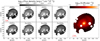 |
Fig. A.1 Left: Flux maps for NGC 1268 in various CFHT and Euclid bands. Right: Stellar mass density map obtained after SED fitting. |
Appendix A.8 Euclid view of known jellyfish galaxies in the Perseus cluster
Two star-forming perturbed galaxies, UGC 2665 (49:51:50.7, 41:38:07) and MCG +07-07-070 (50:05:30.9, 41:38:27) are included within the Euclid ERO images of the Perseus cluster. These objects are characterised by filamentary dusty and stellar structures escaping from their stellar discs, such as those observed in a few cluster objects with available HST data (Kenney et al. 2015; Abramson et al. 2016; Cramer et al. 2019). The two galaxies also have extended radio continuum tails of cometary shape (Roberts et al. 2022a). All this observational evidence suggests that the two galaxies are undergoing a ram-pressure-stripping event (Boselli et al. 2022b). We use the optical and NIR imaging data of extraordinary quality gathered during the Euclid ERO programme of the Perseus cluster to study the impact of the perturbing process on the galaxy properties down to scales of 50–100 pc. The data are first used to identify the dominant perturbing mechanism, hydrodynamical versus gravitational, since the two processes have different effects on the stellar component at very low surface brightness levels, such as those reached by Euclid. We then compare the observed colours of the filamentary structures formed during the interaction to date their epoch of formation with the purpose of posing strong observational constraints on models and simulations. Finally, we can discuss the possible impact that Euclid can have on local studies of galaxy evolution in rich environments thanks to its extraordinary image quality in terms of sensitivity to LSB emission and angular resolution.
Appendix A.9 The density and colour profiles of the far outskirts of galaxies
The high spatial resolution of Euclid offers an unprecedented view of the Perseus cluster with a FoV large enough to encompass a wide range of environments, from field galaxies to groups and galaxies in the cluster itself, each harbouring massive disc galaxies with stellar masses exceeding 1010 M⊙. Euclid’s advanced VIS and NISP cameras provide us with a unique opportunity to explore the detailed stellar structures of the galactic outer discs, thanks to their depth in the optical and NIR domains. The depth and uniformity of the imaging coverage is unequalled for a survey covering both a cluster and field galaxies. Traditionally, the luminosity profiles of disc galaxies have been described by a single exponential (de Vaucouleurs 1959), but over the years observations have been challenging this first model, revealing a more complex reality characterised (at the next level of approximation) by double exponentials (Erwin et al. 2005; Pohlen & Trujillo 2006). Simulations suggest that truncated profiles may stem from internal dynamical processes within the discs, such as Lindblad resonance or star-formation thresholds (Kennicutt 1989), while the origins of anti-truncations remain elusive. These outer disc profiles serve as cosmic fingerprints, offering insights into their late-stage assembly processes (Gutiérrez et al. 2011) and the influence of dark matter halos, sculpted by the surrounding cosmic environment.
The analysis of ERO images of the Perseus cluster – which lies within the gigantic Perseus-Pisces filament – unveils a spectrum of profile types, from truncated to anti-truncated, each providing clues about the disc’s composition and evolution. Preliminary studies conducted on clusters such as Coma (Head et al. 2015) and Virgo (Erwin et al. 2012), where evolved discs abound, have yielded ambiguous conclusions regarding the environmental influences. Within the framework of the ERO, Euclid’s resolution and its large FoV offer a promising avenue for pilot studies, providing limited yet sufficient statistics to delve into the intricate interplay between galaxies and their cosmic surroundings.
Appendix A.10 Analysis of the intracluster light and intracluster globular clusters
ICL is a ubiquitous feature in galaxy clusters (e.g. Feldmeier et al. 2004; Kluge et al. 2020; Golden-Marx et al. 2023). Its assembly history is central to understanding the global evolution of the cluster galaxy population, while it can also be a tool to infer the radius of the cluster and even its dark matter distribution (e.g. Montes & Trujillo 2019; Alonso Asensio et al. 2020; Gonzalez et al. 2021; Yoo et al. 2022; Contreras-Santos et al. 2024).
In Kluge et al. (2025), we make a comprehensive study of the ICL and ICGC in the Perseus ERO programme, mapping their distribution and properties out to a radius of 600 kpc from the brightest cluster galaxy (BCG). We estimate that the central 500 kpc of the Perseus cluster is host to 70 000 ± 2800 globular clusters (BCG+ICGCs), with half of them situated at a distance greater than (239 ± 16) kpc, as well as 1.6 × 10¹² L⊙ of BCG+ICL in HE. We use various properties of the ICL and ICGCs to determine that these intracluster stellar components are most likely to have been tidally stripped from the outskirts of massive elliptical galaxies and from the disruption of dwarf galaxies. The ICL and ICGCs share a coherent spatial distribution, and we find that the ICL and ICGC contours on the largest scales are not centred on the BCG, but rather are offset westwards of the BCG core by approximately 60 kpc, in the direction of several bright cluster members.
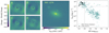 |
Fig. A.2 Left and middle: Example of AGN decomposition, performed with the new package GingaFit, featuring the NGC 1279 X-ray source galaxy. Fitting residuals from single Sérsic, double Sérsic (bulge+disc), PSF+Sérsic, and PSF+double Sérsic models are labelled from A to D. The residuals, shown in linear scale, are normalised to the original image and zoomed-in to show the central area of the galaxy, enclosed in half the Kron Radius. Right: IE AGN luminosity versus total AB magnitude of the host. The sub-populations of objects identified with properties that are similar to the X-ray sources are identified within the boundaries motivated by the faintest of the X-ray sources. |
Appendix A.11 Galaxy morphology from bulge and disc decomposition of galaxies at z < 1
The Hubble sequence has been observed to be in place as early as a billion years after the Big Bang (Ferreira et al. 2023). Thanks to its high spatial resolution and wide FoV, Euclid will enable the morphological analysis of billions of galaxies out to redshifts z ≃ 3 (Euclid Collaboration: Bretonnière et al. 2022), and the reconstruction of the history of the Hubble sequence over most of the age of the Universe.
The ERO Perseus data allow us to test the ability of Euclid images to characterise galaxy morphology for galaxies, mostly in the cluster background, out to redshifts of z ~ 1. In this study, we perform multi-band luminosity model-fitting of the VIS and NISP images with the SourceXtractor++ software (Bertin et al. 2020; Kümmel et al. 2022), whose efficiency was demonstrated in the Euclid Morphology Challenge (Euclid Collaboration: Bretonnière et al. 2023). We perform and analyse the results of several model-fitting runs, using either a single Sérsic profile (Sérsic 1963), or decomposing galaxies as the sum of a Sérsic bulge and an exponential disc. Examining multi-variate distributions of galaxy, bulge and disc properties, we examine the consistencies and biases between the various modelling configurations, and we assess the reliability of the derived structural parameters in these first Euclid data, in the light of the results obtained by the Euclid Morphology Challenge for synthetic galaxy images (Euclid Collaboration: Bretonnière et al. 2023). We are then able to provide robust model-fitting photometry and measure biases between adaptive aperture, single Sérsic, and bulge-disc model photometry, depending on the morphology of the galaxies.
Finally, to build upon the results of Quilley & de Lapparent (2022) that highlighted the Hubble sequence as an inverse evolutionary sequence, along which bulge growth and disc reddening are indicators of the quenching of galaxies, we derive preliminary variations of bulge and disc fluxes, colours, and sizes as a function of redshift out to z ~ 1.
Appendix A.12 Probing AGN activity and host galaxy morphology
The Perseus cluster provided the first and most spectacular example to date of radio-mode AGN feedback from a BCG on the surrounding intracluster medium (Fabian et al. 2003a, 2006; Sanders 2020; Reynolds et al. 2021; Veilleux et al. 2023). Such feedback is expected to be ubiquitous among galaxy clusters throughout the Universe, but is challenging to identify in large numbers. The high-resolution imaging of the EWS opens up the possibility of teasing out point-source AGN emission from host galaxies, and thereby building a census of AGN activity in the Euclid survey. We explore the reliability of this AGN-host decomposition on the members of the Perseus cluster, including the hosts of 13 known X-ray point sources (Santra et al. 2007), which serve as a reference sample. For the structural decomposition (Kim et al. 2008; Bruce et al. 2016; Wittmann et al. 2019; Peng et al. 2010) we carefully account for sources of bias, making sure that our measurements are robust against degeneracies in the multi-dimensional parameter space of galaxy structural properties (Tarsitano et al. 2018). We perform multiple fits of increasing complexity, combining one or multiple Sérsic profiles and PSF components, using our newly developed python package named GingaFit.15
In the fitting residuals (as those shown in the left panels of Fig. A.2), both the single Sérsic (panel A) and the bulge+disc (panel B) models leave a central concentration of light and structure at large radii, arising from the fact that galaxies do not have smooth, axi-symmetric light profiles. In each case, the addition of a point-source component significantly improves the fitting model, whilst also accounting for the point-source residual. In the right panel of Fig. A.2, we show the implied point-source luminosity for each cluster member galaxy, integrated over the IE band, against their host’s absolute magnitudes from the bulge and disc components. We are able to isolate two sub-samples, one within the same luminosity-magnitude range of the X-ray sources, and another low-mass sample with high luminosity. The measurement reliability and nature of the emission of all luminous point sources will be determined in a future paper.
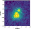 |
Fig. A.3 VIS image of the dual lensed AGN candidate SDSS J032023.93+412131.5 at z = 2.811, showing the nearby companion at |
![$\[0^{\prime \prime}_\cdot65\]$](/articles/aa/full_html/2025/05/aa50808-24/aa50808-24-eq75.png)
Appendix A.13 Dual/lensed QSO candidates at sub-arcsecond separations
During their life, galaxies experience a number of major and minor mergers with other galaxies. The supermassive black holes (SMBHs) present in the centres of most massive galaxies merge together with their hosts, creating a SMBH pair that slowly reduces its separation and eventually merges, creating a burst of gravitational waves (GW; e.g. Colpi 2014). During the in-spiralling phase, which can last gigayears (e.g. Volonteri et al. 2022), these pairs can be detected as dual AGN at kiloparsec separations.
The appearance of two or more QSOs at the same redshift and close separations can also be due to strong gravitational lensing of a single QSO due a foreground galaxy, producing multiple images of the background source. These are systems or great relevance in many fields of the astrophysics (e.g. Shajib et al. 2022).
Detecting these rare systems of dual or lensed QSOs is challenging because it requires high-resolution imaging over large parts of the sky, and only a small number of confirmed such systems have been discovered, especially outside the local universe (De Rosa et al. 2019; Mannucci et al. 2023). Recently, several techniques based on the ESA Gaia satellite have been proposed to select homogeneous samples of dual/lensed AGN candidates at sub-arcsecond separations (e.g. Lemon et al. 2017; Hwang et al. 2020; Mannucci et al. 2022). With its large FoV, superb spatial resolution, and high sensitivity, the Euclid VIS camera can outperform the previous techniques based on optical data and provide large samples of dual/lensed AGN candidates, that is, AGN with nearby companions.
One such system have already been discovered by examining the eight known QSO with z > 0.1 covered by the VIS image of the Perseus cluster. One of them, SDSS J032023.93+412131.5, a QSO at z = 2.811 discovered by the SDSS (Lyke et al. 2020), shows a nearby companion at ![$\[0^{\prime \prime}_\cdot65\]$](/articles/aa/full_html/2025/05/aa50808-24/aa50808-24-eq76.png) of separation and 3.1 magnitude fainter than the primary component, see Fig. A.3. This system in unresolved in the Euclid NISP image, characterised by a much lower spatial resolution. Preliminary highresolution NIR imaging with LBT (Ulivi et al., in prep), has revealed that the two objects have very similar optical-to-nearIR colours, indicating that the faint component is likely to be a secondary QSO in either a dual or a strongly lensed system. In the former case, the projected separation between the two component would be ~5.2 kpc.
of separation and 3.1 magnitude fainter than the primary component, see Fig. A.3. This system in unresolved in the Euclid NISP image, characterised by a much lower spatial resolution. Preliminary highresolution NIR imaging with LBT (Ulivi et al., in prep), has revealed that the two objects have very similar optical-to-nearIR colours, indicating that the faint component is likely to be a secondary QSO in either a dual or a strongly lensed system. In the former case, the projected separation between the two component would be ~5.2 kpc.
Appendix A.14 Properties of the interstellar medium: Albedo derivation from the optical to the NIR
The ERO Perseus data allow us to test the idea of using the Euclid images to study the structure of the Galactic interstellar medium (ISM) as well as the properties of interstellar dust. These micron-size solid particles absorb starlight, producing absorption, AV, and reddening, E(B − V), in the visible (and NIR), as well as a wide emission spectrum extending from the mid-IR to millimetre wavelengths. These signatures have been extensively used to understand the nature of interstellar dust, and also as tracers of the ISM structure. The underlying idea is that dust and gas are well mixed, in every phase of the ISM (Boulanger & Perault 1988).
In addition to absorption, a significant fraction of the starlight impinging on micron-size dust grains is scattered off their surfaces. Given their size and shape, the scattering is observed in the UV through the NIR, with an expected maximum around λ = 1 μm (Gordon 2004; Jones et al. 2017). This scattered light, historically dubbed diffuse Galactic light (DGL) has been known for several decades (Elvey & Roach 1937; Sandage 1976), but it is only recently that it has been used, such as absorption and emission, as a tracer of interstellar structure (Boissier et al. 2015; Miville-Deschênes et al. 2016; Mattila et al. 2018; Román et al. 2020; Liu et al. 2023). An important difference with emission and absorption is that the scattered light amplitude depends on the 3D structure of the radiation field because stellar photons are predominantly scattered in the forward direction. Therefore, in regions with very anisotropic radiation fields, the scattered light image will give a distorted picture of the interstellar density field. Fortunately most of the sky at high Galactic latitude is composed of diffuse interstellar clouds that are not forming stars and are illuminated by the general interstellar radiation field that can be considered to be close to isotropic. In this case, large area mapping of diffuse areas of the sky in the optical and NIR with very high angular resolution offers the opportunity to map the ISM structure down to AU scales over hundreds of parsecs.
The Perseus cluster field is a good test case for this. It is at intermediate latitude (b = −13°) with a moderate column density of NH ≃ 1.4 × 1021 cm−2 using the E(B − V) ≃ 0.16 estimate of Planck Collaboration XI (2014) in this area and the E(B − V)/NH conversion factor of Lenz et al. (2017). This corresponds to the translucent part of the interstellar medium (AV ≃ 0.5) where matter is expected to be mostly atomic. According to the THEMIS dust model (Jones et al. 2017), the dust scattering should be maximum in the Euclid JE band. However, these theoretical estimates are based on very little data (see the review by Gordon 2004) and the exact shape of the scattered light spectrum should vary locally, since it contains information about dust shape, composition, and sizes. The combination of Euclid’s four bands, coupled with deep complementary optical u, g, r, i, and z ground-based CFHT data, provides a powerful wavelength range to study the DGL. In particular, combining scattering and emission offers a great opportunity to improve current dust models (e.g. Zhang et al. 2023).
Appendix B Structural parameters
Appendix B.1 AutoProf and AstroPhot parameters
The photometry of galaxies identified as cluster members is carried out with AutoProf for the bright galaxies and a combination of AstroPhot and Galfit for the dwarf galaxies (Marleau et al. 2025). The codes are run on a limited portion of the image: the size of the cutouts varied for all the dwarfs depending on their effective radius, as described in Marleau et al. (2025). For the bright galaxies, the cutouts also varied in size, ranging from 1000 × 1000, 2000 × 2000, 4000 × 4000, and 8000 × 8000 VIS pixels, depending on their angular scale on the sky, the tile size being optimised to facilitate accurate sky background estimation. Only the two largest galaxies in the cluster, NGC 1272 and NGC 1275, required a tile size of 8000 × 8000 VIS pixels, as illustrated in Fig. B.1.
For the dwarf galaxies, the galaxy modelling was initially performed using AutoProf (Stone et al. 2021) to obtain a first estimate of the structural parameters. These initial estimates were then used as input to both Galfit (Peng et al. 2010) and AstroPhot (Stone et al. 2023). The details of the dwarf galaxy modelling procedure and results are presented in Marleau et al. (2025).
For the bright galaxy sample, after initially selecting galaxies based on their apparent size, a second sorting was conducted based on the proximity of the galaxies to each other. This proximity significantly influenced the choice of photometric extraction tool. AutoProf was utilised for relatively isolated galaxies, where their outermost isophotes do not significantly overlap with those of neighbouring galaxies. Conversely, AstroPhot is preferred for galaxies that are in close proximity to each other.
Once the tiles were extracted, the photometry of isolated galaxies was determined using the AutoProf tool. To minimise contamination from MW stars in the VIS photometry calculations, a star mask was created from each segmentation map generated by SourceExtractor. AutoProf then took this mask along with the galaxy image from the corresponding tile as inputs. AutoProf processed each galaxy to provide a detailed surface brightness profile, after fitting isophotes leading to an azimutally averaged profile averaging the pixels along the isophotes. Output products included characteristic fit parameters such as sky background estimation, position angle, and mean ellipticity, among others. Figure B.1 displays examples of profiles generated by AutoProf. Additionally, a Sérsic model fit to the 1D profile was performed to derive the Sérsic index. Other photometric parameters extracted include total magnitude and effective radius, providing a comprehensive picture of each galaxy.
The remaining galaxies found in a crowded environment (i.e. 34 of the 137 bright galaxies) were analysed using the AstroPhot tool, which provides a range of modelling options. For these galaxies, simple Sérsic profiles were initially fitted. Tiles of 4000 pixels × 4000 pixels were preferred, to ensure ample sky background for accurate photometry estimation in these complex areas. To initialise AstroPhot, star masking was conducted using the same approach as with AutoProf, employing segmentation maps and parameters from SourceExtractor, such as ellipticity, position angle, and estimated flux for each galaxy. Sérsic models were then initialised over 100 × 100 pixel windows, typically encompassing the galaxy’s core. The process began with a first iteration using an iterative method to refine the model. This was followed by a second iteration that utilised the parameters from the first iteration but expanded the analysis to a 1000 × 1000 pixel window. Ultimately, a Sérsic profile was fit for each galaxy, detailing associated morphological and photometric parameters, as depicted in Fig. B.2. The results of the photometric analysis for bright galaxies are described in the tables of the Appendix C.
Appendix B.2 Comparison with other codes
We first made a comparison of the SourceExtractor magnitudes extracted from the ring-filtered images and used in Sect. 7 with those measured using AutoProf/AstroPhot. The two sets of data agree within 0.1 mag, with a dispersion of 0.3. Since SourceExtractor magnitudes are consistently used to derive all the colours in the SED fitting procedure, we do not expect any major effect in the derivation of the stellar masses.
Other photometry software codes are available for comparison. In Stone et al. (2021), AutoProf has been compared to PHOTUTILS, XVISTA, and Galfit. In this appendix, an additional comparison is made with the Archangel pipeline (Schombert 2007; Schombert & Smith 2012) using the same specific Euclid ERO data. Previously, the Archangel software had been adapted for Spitzer space observations as described in detail in Sorce et al. (2012). For the comparisons in this appendix, it was further modified to be applied to Euclid data. Briefly, Archangel performs the masking of stars and flaws. Subsequently, it replaces masked regions by mean isophote values. Ellipses are then fit to isophotes with increasing radii. The 2D information is compressed into uni-dimensional surface brightness and magnitude growth curves. Other parameters such as extrapolated magnitudes, are finally derived. Archangel was run once on each galaxy of our test sample. We did not modify the parameters between elliptical, spiral, and dwarf galaxies so as not to bias the comparisons. In any case, Sorce et al. (2012) showed that the major contribution to the magnitude uncertainties for space-based observations is the setting of the sky level. Furthermore, Sorce et al. (2012) and Sorce et al. (2014) demonstrated the agreement between magnitudes obtained with the Spitzer-adapted version of Archangel and other alternative pipelines, such as the software developed for the GALEX Large Galaxy Atlas16 (GLGA, Seibert 2007) or for the Spitzer Survey of Stellar Structure in Galaxies (S4G, Sheth et al. 2010). The sky setting was identified as the cause of any difference between a few outliers.
Following the main analysis of the paper, the zero point is set to 30.13 (30) for the IE (YE, JE, HE) bands, the pixel size is ![$\[0^{\prime \prime}_\cdot1\]$](/articles/aa/full_html/2025/05/aa50808-24/aa50808-24-eq77.png) and magnitudes are given in the AB system. In this appendix, detailed comparisons are presented for an elliptical, a spiral, and a dwarf galaxy, to emphasise the agreement between both software codes. Figure B.3 shows the surface brightness profile (blue solid and dashed lines) and the curve of growth (red solid and orange dashed lines) obtained for the three galaxies using Archangel (solid lines) and AutoProf (dashed lines). There is an agreement between the surface brightness profiles out to the edges of the galaxies. The curves of growth tend to increase faster with AutoProf but converge asymptotically to the same magnitude as those obtained with Archangel. Axis ratios and position angles derived with both codes are similar though. The curves of growth thus differ only by the radius definition. Table B.1 summarises the magnitudes in the four Euclid bands obtained with both codes for the three galaxies, confirming the agreement.
and magnitudes are given in the AB system. In this appendix, detailed comparisons are presented for an elliptical, a spiral, and a dwarf galaxy, to emphasise the agreement between both software codes. Figure B.3 shows the surface brightness profile (blue solid and dashed lines) and the curve of growth (red solid and orange dashed lines) obtained for the three galaxies using Archangel (solid lines) and AutoProf (dashed lines). There is an agreement between the surface brightness profiles out to the edges of the galaxies. The curves of growth tend to increase faster with AutoProf but converge asymptotically to the same magnitude as those obtained with Archangel. Axis ratios and position angles derived with both codes are similar though. The curves of growth thus differ only by the radius definition. Table B.1 summarises the magnitudes in the four Euclid bands obtained with both codes for the three galaxies, confirming the agreement.
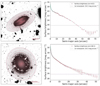 |
Fig. B.1 Examples of AutoProf radial profile extraction on VIS data to derive photometric and morphological properties. Top left: UGC 02665 isophote fitting on an 2000 pixel × 2000 pixel pixel cutout (200″ × 200″, red angular scale on the image: 30″). Top right: Radial surface brightness profile for UGC 02665, showing a dip at r = 60″ due to overlap with neighbours, marking the photometry’s limit. Bottom left: WISEAJ031858.26 +414208.7 isophote fitting on a 2000 pixel × 2000 pixel cutout (200″ × 200″, red angular scale on the image: 30″). Bottom right: Radial surface brightness profile for NGC 1281, reaching down to 30.1 mag arcsec−2 at r = 100″ despite the proximity of a bright star. Cyan and red points on the radial profiles refer to the colours of isophotes in the associated AutoProf visual, which help guide the eye when comparing plots. |
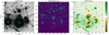 |
Fig. B.2 Example of an AstroPhot fitting process on VIS data to derive photometric and morphological properties. Left: Input image (4000 pixel × 4000 pixel pixel cutout, 400″ × 400″) featuring multiple overlapping galaxies from the Perseus cluster, namely NGC 1270, NGC 1268, NGC 1267, and CGCG540-089. Centre: Segmentation map of the image by SourceExtractor (scale in pixels). Right: Residual image (image minus models) for the initial fit, this gets substantially improved upon iterating. |
Magnitudes in the four Euclid bands.
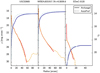 |
Fig. B.3 Surface-brightness profiles (red and orange lines, and left axis) and curves of growth (blue lines and right axis) obtained for three galaxies whose names are given at the top of each panel. The photometry has been performed with AutoProf (dashed lines) and Archangel (solid lines). There is a good agreement between both software codes. |
Appendix C Photometric tables of bright galaxies
This section presents nine tables offering a complete overview of the catalogue, which is available as supplementary material at the Strasbourg astronomical Data Centre (CDS). The tables are as follows.
Table C.1: Complete list of parameters extracted for Tables C.3 to C.5, along with their descriptions and associated table indexes.
Table C.2: Complete list of parameters extracted for Tables C.6–C.9, along with their descriptions and associated table indexes.
Table C.3: primary data from VIS photometry.
Table C.4: associated errors for the primary data catalogue.
Table C.5: redshift and extinction corrections.
Table C.6: magnitudes within one effective radius (Re) in VIS and NISP bands.
Table C.7: associated errors of the 1 Re magnitudes catalogue. Table C.8: magnitudes using VIS photometry to constrain NISP photometry.
Table C.9: associated errors of the forced magnitudes.
Primary data from VIS photometry.
Associated errors for the primary data catalogue
Redshift and extinction corrections.
Magnitudes within 1 effective radius in VIS and NISP bands.
Associated errors of the 1 Re magnitudes catalogue.
Magnitudes using VIS photometry to constrain NISP photometry.
Associated errors of the forced magnitudes.
Appendix D SourceExtractor parameters
We report in Table D.1 the main parameters of SourceExtractor on the CFHT i band. Similar files for the NISP and VIS bands are available with the public distribution of the catalogues.17. The list of output parameters is provided in the appendix of Cuillandre et al. (2025).
SourceExtractor input configuration for the CFHT i band.
References
- Aaronson, M., Gordon, G., Mould, J., Olszewski, E., & Suntzeff, N. 1985, ApJ, 296, L7 [Google Scholar]
- Abdurro’uf, Lin, Y.-T., Wu, P.-F., & Akiyama, M. 2021, ApJS, 254, 15 [CrossRef] [Google Scholar]
- Abdurro’uf, Lin, Y.-T., Hirashita, H., et al. 2022a, ApJ, 926, 81 [Google Scholar]
- Abdurro’uf, Lin, Y.-T., Wu, P.-F., & Akiyama, M. 2022b, piXedfit: Analyze spatially resolved SEDs of galaxies, Astrophysics Source Code Library [record ascl:2207.033] [Google Scholar]
- Abramson, A., Kenney, J., Crowl, H., & Tal, T. 2016, AJ, 152, 32 [Google Scholar]
- Adami, C., Durret, F., Mazure, A., et al. 2007, A&A, 462, 411 [NASA ADS] [CrossRef] [EDP Sciences] [Google Scholar]
- Aguerri, J. A. L., Varela, A. M., Prieto, M., & Muñoz-Tuñón, C. 2000, AJ, 119, 1638 [NASA ADS] [CrossRef] [Google Scholar]
- Aguerri, J. A. L., Girardi, M., Agulli, I., et al. 2020, MNRAS, 494, 1681 [NASA ADS] [CrossRef] [Google Scholar]
- Aharonian, F. A., Akamatsu, H., Akimoto, F., et al. 2017, ApJ, 837, L15 [NASA ADS] [CrossRef] [Google Scholar]
- Alonso Asensio, I., Dalla Vecchia, C., Bahé, Y. M., Barnes, D. J., & Kay, S. T. 2020, MNRAS, 494, 1859 [CrossRef] [Google Scholar]
- Amorisco, N. C., Monachesi, A., Agnello, A., & White, S. D. M. 2018, MNRAS, 475, 4235 [NASA ADS] [CrossRef] [Google Scholar]
- Andreon, S. 1994, A&A, 284, 801 [NASA ADS] [Google Scholar]
- Andreon, S., & Cuillandre, J. C. 2002, ApJ, 569, 144 [Google Scholar]
- Andreon, S., Cuillandre, J. C., Puddu, E., & Mellier, Y. 2006, MNRAS, 372, 60 [Google Scholar]
- Baldry, I. K., Driver, S. P., Loveday, J., et al. 2012, MNRAS, 421, 621 [NASA ADS] [Google Scholar]
- Balogh, M. L., Christlein, D., Zabludoff, A. I., & Zaritsky, D. 2001, ApJ, 557, 117 [NASA ADS] [CrossRef] [Google Scholar]
- Barkhouse, W. A., Yee, H. K. C., & López-Cruz, O. 2007, ApJ, 671, 1471 [Google Scholar]
- Batuski, D. J., & Burns, J. O. 1985, AJ, 90, 1413 [Google Scholar]
- Bautz, L. P., & Morgan, W. W. 1970, ApJ, 162, L149 [NASA ADS] [CrossRef] [Google Scholar]
- Beijersbergen, M., Hoekstra, H., van Dokkum, P. G., & van der Hulst, T. 2002, MNRAS, 329, 385 [NASA ADS] [CrossRef] [Google Scholar]
- Bekki, K., Couch, W. J., Drinkwater, M. J., & Shioya, Y. 2003, MNRAS, 344, 399 [NASA ADS] [CrossRef] [Google Scholar]
- Bell, E. F., McIntosh, D. H., Katz, N., & Weinberg, M. D. 2003, ApJS, 149, 289 [Google Scholar]
- Benson, A. J., Bower, R. G., Frenk, C. S., et al. 2003, ApJ, 599, 38 [NASA ADS] [CrossRef] [Google Scholar]
- Bertin, E. 2011, in Astronomical Society of the Pacific Conference Series, 442, Astronomical Data Analysis Software and Systems XX, eds. I. N. Evans, A. Accomazzi, D. J. Mink, & A. H. Rots, 435 [Google Scholar]
- Bertin, E., & Arnouts, S. 1996, A&AS, 117, 393 [NASA ADS] [CrossRef] [EDP Sciences] [Google Scholar]
- Bertin, E., Mellier, Y., Radovich, M., et al. 2002, in Astronomical Society of the Pacific Conference Series, 281, Astronomical Data Analysis Software and Systems XI, eds. D. A. Bohlender, D. Durand, & T. H. Handley, 228 [Google Scholar]
- Bertin, E., Schefer, M., Apostolakos, N., et al. 2020, in ASP Conference Series, 527, Astronomical Data Analysis Software and Systems XXIX, eds. R. Pizzo, E. R. Deul, J. D. Mol, J. de Plaa, & H. Verkouter, 461 [Google Scholar]
- Binggeli, B., & Jerjen, H. 1998, A&A, 333, 17 [NASA ADS] [Google Scholar]
- Binggeli, B., Sandage, A., & Tammann, G. A. 1985, AJ, 90, 1681 [Google Scholar]
- Binggeli, B., Tarenghi, M., & Sandage, A. 1990, A&A, 228, 42 [NASA ADS] [Google Scholar]
- Biviano, A., Durret, F., Gerbal, D., et al. 1995, A&A, 297, 610 [NASA ADS] [Google Scholar]
- Blakeslee, J. P., Jensen, J. B., Ma, C.-P., Milne, P. A., & Greene, J. E. 2021, ApJ, 911, 65 [NASA ADS] [CrossRef] [Google Scholar]
- Blanton, M. R., Hogg, D. W., Bahcall, N. A., et al. 2003, ApJ, 592, 819 [Google Scholar]
- Blanton, M. R., Eisenstein, D., Hogg, D. W., Schlegel, D. J., & Brinkmann, J. 2005a, ApJ, 629, 143 [Google Scholar]
- Blanton, M. R., Lupton, R. H., Schlegel, D. J., et al. 2005b, ApJ, 631, 208 [Google Scholar]
- Boehringer, H., Voges, W., Fabian, A. C., Edge, A. C., & Neumann, D. M. 1993, MNRAS, 264, L25 [NASA ADS] [CrossRef] [Google Scholar]
- Boissier, S., Boselli, A., Voyer, E., et al. 2015, A&A, 579, A29 [NASA ADS] [CrossRef] [EDP Sciences] [Google Scholar]
- Bolzonella, M., Miralles, J. M., & Pelló, R. 2000, A&A, 363, 476 [NASA ADS] [Google Scholar]
- Bolzonella, M., Kovač, K., Pozzetti, L., et al. 2010, A&A, 524, A76 [NASA ADS] [CrossRef] [EDP Sciences] [Google Scholar]
- Boselli, A., & Gavazzi, G. 2006, PASP, 118, 517 [Google Scholar]
- Boselli, A., & Gavazzi, G. 2014, A&A Rev., 22, 74 [CrossRef] [Google Scholar]
- Boselli, A., Tuffs, R. J., Gavazzi, G., Hippelein, H., & Pierini, D. 1997, A&AS, 121, 507 [NASA ADS] [CrossRef] [EDP Sciences] [Google Scholar]
- Boselli, A., Gavazzi, G., Franzetti, P., Pierini, D., & Scodeggio, M. 2000, A&AS, 142, 73 [NASA ADS] [CrossRef] [EDP Sciences] [Google Scholar]
- Boselli, A., Iglesias-Páramo, J., Vílchez, J. M., & Gavazzi, G. 2002, A&A, 386, 134 [NASA ADS] [CrossRef] [EDP Sciences] [Google Scholar]
- Boselli, A., Boissier, S., Cortese, L., & Gavazzi, G. 2008a, ApJ, 674, 742 [Google Scholar]
- Boselli, A., Boissier, S., Cortese, L., & Gavazzi, G. 2008b, A&A, 489, 1015 [CrossRef] [EDP Sciences] [Google Scholar]
- Boselli, A., Voyer, E., Boissier, S., et al. 2014, A&A, 570, A69 [NASA ADS] [CrossRef] [EDP Sciences] [Google Scholar]
- Boselli, A., Boissier, S., Voyer, E., et al. 2016, A&A, 585, A2 [Google Scholar]
- Boselli, A., Fossati, M., Ferrarese, L., et al. 2018, A&A, 614, A56 [NASA ADS] [CrossRef] [EDP Sciences] [Google Scholar]
- Boselli, A., Fossati, M., Longobardi, A., et al. 2022a, A&A, 659, A46 [NASA ADS] [CrossRef] [EDP Sciences] [Google Scholar]
- Boselli, A., Fossati, M., & Sun, M. 2022b, A&A Rev., 30, 3 [Google Scholar]
- Boselli, A., Fossati, M., Côté, P., et al. 2023, A&A, 675, A123 [NASA ADS] [CrossRef] [EDP Sciences] [Google Scholar]
- Boué, G., Adami, C., Durret, F., Mamon, G. A., & Cayatte, V. 2008, A&A, 479, 335 [NASA ADS] [CrossRef] [EDP Sciences] [Google Scholar]
- Boulanger, F., & Perault, M. 1988, ApJ, 330, 964 [NASA ADS] [CrossRef] [Google Scholar]
- Bower, R. G., Lucey, J. R., & Ellis, R. S. 1992, MNRAS, 254, 589 [NASA ADS] [CrossRef] [Google Scholar]
- Boyarsky, A., Ruchayskiy, O., Iakubovskyi, D., & Franse, J. 2014, Phys. Rev. Lett., 113, 251301 [NASA ADS] [CrossRef] [Google Scholar]
- Bruce, V. A., Dunlop, J. S., Mortlock, A., et al. 2016, MNRAS, 458, 2391 [CrossRef] [Google Scholar]
- Brunzendorf, J., & Meusinger, H. 1999, A&AS, 139, 141 [NASA ADS] [CrossRef] [EDP Sciences] [Google Scholar]
- Bruzual, G., & Charlot, S. 2003, MNRAS, 344, 1000 [NASA ADS] [CrossRef] [Google Scholar]
- Buitrago, F., & Trujillo, I. 2024, A&A, 682, A110 [NASA ADS] [CrossRef] [EDP Sciences] [Google Scholar]
- Buitrago, F., Ferreras, I., Kelvin, L. S., et al. 2018, A&A, 619, A137 [NASA ADS] [CrossRef] [EDP Sciences] [Google Scholar]
- Bullock, J. S., & Boylan-Kolchin, M. 2017, ARA&A, 55, 343 [Google Scholar]
- Cantiello, M., & Blakeslee, J. P. 2023, arXiv e-prints [arXiv:2307.03116] [Google Scholar]
- Cantiello, M., Raimondo, G., Brocato, E., & Capaccioli, M. 2003, AJ, 125, 2783 [Google Scholar]
- Cantiello, M., Blakeslee, J. P., Ferrarese, L., et al. 2018, ApJ, 856, 126 [Google Scholar]
- Cappellari, M. 2016, ARA&A, 54, 597 [Google Scholar]
- Cappellari, M., Emsellem, E., Krajnović, D., et al. 2011, MNRAS, 416, 1680 [Google Scholar]
- Carleton, T., Errani, R., Cooper, M., et al. 2019, MNRAS, 485, 382 [NASA ADS] [CrossRef] [Google Scholar]
- Carlsten, S. G., Greene, J. E., Beaton, R. L., & Greco, J. P. 2022, ApJ, 927, 44 [NASA ADS] [CrossRef] [Google Scholar]
- Chabrier, G. 2003, PASP, 115, 763 [Google Scholar]
- Chincarini, G., & Rood, H. J. 1971, ApJ, 168, 321 [NASA ADS] [CrossRef] [Google Scholar]
- Chincarini, G. L., Giovanelli, R., & Haynes, M. P. 1983, A&A, 121, 5 [Google Scholar]
- Churazov, E., Forman, W., Jones, C., & Böhringer, H. 2003, ApJ, 590, 225 [NASA ADS] [CrossRef] [Google Scholar]
- Cole, S., Lacey, C. G., Baugh, C. M., & Frenk, C. S. 2000, MNRAS, 319, 168 [Google Scholar]
- Cole, S., Norberg, P., Baugh, C. M., et al. 2001, MNRAS, 326, 255 [NASA ADS] [CrossRef] [Google Scholar]
- Colpi, M. 2014, Space Sci. Rev., 183, 189 [Google Scholar]
- Comerón, S., Trujillo, I., Cappellari, M., et al. 2023, A&A, 675, A143 [NASA ADS] [CrossRef] [EDP Sciences] [Google Scholar]
- Conroy, C., & Gunn, J. E. 2010, ApJ, 712, 833 [Google Scholar]
- Conselice, C. J., Gallagher, John S., I., & Wyse, R. F. G. 2001, AJ, 122, 2281 [NASA ADS] [CrossRef] [Google Scholar]
- Contreras-Santos, A., Knebe, A., Cui, W., et al. 2024, A&A, 683, A59 [NASA ADS] [CrossRef] [EDP Sciences] [Google Scholar]
- Cramer, W. J., Kenney, J. D. P., Sun, M., et al. 2019, ApJ, 870, 63 [Google Scholar]
- Cropper, M., Pottinger, S., Niemi, S., et al. 2016, SPIE Conf. Ser., 9904, 99040Q [NASA ADS] [Google Scholar]
- Csabai, I., Budavári, T., Connolly, A. J., et al. 2003, AJ, 125, 580 [Google Scholar]
- Csabai, I., Dobos, L., Trencséni, M., et al. 2007, Astron. Nachr., 328, 852 [NASA ADS] [CrossRef] [Google Scholar]
- Cuillandre, J.-C., Bertin, E., Bolzonella, M., et al. 2025, A&A, 697, A6 (Euclid on Sky SI) [Google Scholar]
- Czekaj, M. A. 2012, PhD thesis, University of Barcelona, Spain, Galaxy evolution: A new version of the Besançon galaxy model constrained with Tycho data [Google Scholar]
- Daddi, E., Cimatti, A., Renzini, A., et al. 2004, ApJ, 617, 746 [NASA ADS] [CrossRef] [Google Scholar]
- de Filippis, E., Paolillo, M., Longo, G., et al. 2011, MNRAS, 414, 2771 [Google Scholar]
- De Lucia, G., & Blaizot, J. 2007, MNRAS, 375, 2 [Google Scholar]
- De Lucia, G., Poggianti, B. M., Aragón-Salamanca, A., et al. 2007, MNRAS, 374, 809 [Google Scholar]
- De Lucia, G., Poggianti, B. M., Halliday, C., et al. 2009, MNRAS, 400, 68 [NASA ADS] [CrossRef] [Google Scholar]
- de Propris, R., Eisenhardt, P. R., Stanford, S. A., & Dickinson, M. 1998, ApJ, 503, L45 [NASA ADS] [CrossRef] [Google Scholar]
- De Propris, R., Colless, M., Driver, S. P., et al. 2003, MNRAS, 342, 725 [NASA ADS] [CrossRef] [Google Scholar]
- De Rosa, A., Vignali, C., Bogdanović, T., et al. 2019, New A Rev., 86, 101525 [NASA ADS] [CrossRef] [Google Scholar]
- Dekel, A., & Birnboim, Y. 2006, MNRAS, 368, 2 [NASA ADS] [CrossRef] [Google Scholar]
- de Vaucouleurs, G. 1959, Handbuch Phys., 53, 275 [Google Scholar]
- Di Cintio, A., Brook, C. B., Dutton, A. A., et al. 2017, MNRAS, 466, L1 [NASA ADS] [CrossRef] [Google Scholar]
- Dressler, A. 1980a, ApJS, 42, 565 [Google Scholar]
- Dressler, A. 1980b, ApJ, 236, 351 [Google Scholar]
- Dressler, A., Oemler, Augustus, J., Couch, W. J., et al. 1997, ApJ, 490, 577 [NASA ADS] [CrossRef] [Google Scholar]
- Drinkwater, M. J., Gregg, M. D., Hilker, M., et al. 2003, Nature, 423, 519 [CrossRef] [Google Scholar]
- Driver, S. P., Andrews, S. K., Davies, L. J., et al. 2016, ApJ, 827, 108 [CrossRef] [Google Scholar]
- Duc, P.-A., Cuillandre, J.-C., Karabal, E., et al. 2015, MNRAS, 446, 120 [Google Scholar]
- Durret, F., Gerbal, D., Lobo, C., & Pichon, C. 1999, A&A, 343, 760 [NASA ADS] [Google Scholar]
- Edge, A. C., Stewart, G. C., Fabian, A. C., & Arnaud, K. A. 1990, MNRAS, 245, 559 [NASA ADS] [Google Scholar]
- Efstathiou, G., Ellis, R. S., & Peterson, B. A. 1988, MNRAS, 232, 431 [Google Scholar]
- Elvey, C. T., & Roach, F. E. 1937, ApJ, 85, 213 [Google Scholar]
- Erwin, P. 2015, ApJ, 799, 226 [Google Scholar]
- Erwin, P., Beckman, J. E., & Pohlen, M. 2005, ApJ, 626, L81 [Google Scholar]
- Erwin, P., Gutiérrez, L., & Beckman, J. E. 2012, ApJ, 744, L11 [NASA ADS] [CrossRef] [Google Scholar]
- Estrada, N., Mercurio, A., Vulcani, B., et al. 2023, A&A, 671, A146 [NASA ADS] [CrossRef] [EDP Sciences] [Google Scholar]
- Euclid Collaboration (Desprez, G., et al.) 2020, A&A, 644, A31 [EDP Sciences] [Google Scholar]
- Euclid Collaboration (Bretonnière, H., et al.) 2022, A&A, 657, A90 [CrossRef] [EDP Sciences] [Google Scholar]
- Euclid Collaboration (Scaramella, R., et al.) 2022, A&A, 662, A112 [NASA ADS] [CrossRef] [EDP Sciences] [Google Scholar]
- Euclid Collaboration (Schirmer, M., et al.) 2022, A&A, 662, A92 [NASA ADS] [CrossRef] [EDP Sciences] [Google Scholar]
- Euclid Collaboration (Bretonnière, H., et al.) 2023, A&A, 671, A102 [NASA ADS] [CrossRef] [EDP Sciences] [Google Scholar]
- Euclid Collaboration (Schirmer, M., et al.) 2023, A&A, 675, A142 [Google Scholar]
- Euclid Collaboration (Cropper, M. S., et al.) 2025, A&A, 697, A2 (Euclid on Sky SI) [Google Scholar]
- Euclid Collaboration (Jahnke, K., et al.) 2025, A&A, 697, A3 (Euclid on Sky SI) [Google Scholar]
- Euclid Collaboration (Mellier, Y., et al.) 2025, A&A, 697, A1 (Euclid on Sky SI) [Google Scholar]
- Euclid Early Release Observations 2024, https://doi.org/10.57780/esa-qmocze3 [Google Scholar]
- Faber, S. M., Willmer, C. N. A., Wolf, C., et al. 2007, ApJ, 665, 265 [Google Scholar]
- Fabian, A. C., Sanders, J. S., Allen, S. W., et al. 2003a, MNRAS, 344, L43 [Google Scholar]
- Fabian, A. C., Sanders, J. S., Crawford, C. S., et al. 2003b, MNRAS, 344, L48 [Google Scholar]
- Fabian, A. C., Sanders, J. S., Taylor, G. B., et al. 2006, MNRAS, 366, 417 [NASA ADS] [CrossRef] [Google Scholar]
- Feldmeier, J. J., Mihos, J. C., Morrison, H. L., et al. 2004, ApJ, 609, 617 [Google Scholar]
- Ferguson, H. C., & Binggeli, B. 1994, A&A Rev., 6, 67 [NASA ADS] [CrossRef] [Google Scholar]
- Fernández-Iglesias, J., Buitrago, F., & Sahelices, B. 2024, A&A, 683, A145 [NASA ADS] [CrossRef] [EDP Sciences] [Google Scholar]
- Feroz, F., & Hobson, M. P. 2008, MNRAS, 384, 449 [NASA ADS] [CrossRef] [Google Scholar]
- Feroz, F., Hobson, M. P., Cameron, E., & Pettitt, A. N. 2019, Open J. Astrophys., 2, 10 [Google Scholar]
- Ferrarese, L., Côté, P., Cuillandre, J.-C., et al. 2012, ApJS, 200, 4 [Google Scholar]
- Ferrarese, L., Côté, P., Sánchez-Janssen, R., et al. 2016, ApJ, 824, 10 [NASA ADS] [CrossRef] [Google Scholar]
- Ferrarese, L., Côté, P., MacArthur, L. A., et al. 2020, ApJ, 890, 128 [Google Scholar]
- Ferré-Mateu, A., Trujillo, I., Martín-Navarro, I., et al. 2017, MNRAS, 467, 1929 [NASA ADS] [Google Scholar]
- Ferreira, L., Conselice, C. J., Sazonova, E., et al. 2023, ApJ, 955, 94 [NASA ADS] [CrossRef] [Google Scholar]
- Fioc, M., & Rocca-Volmerange, B. 1997, A&A, 326, 950 [NASA ADS] [Google Scholar]
- Fossati, M., Fumagalli, M., Lofthouse, E. K., et al. 2021, MNRAS, 503, 3044 [NASA ADS] [CrossRef] [Google Scholar]
- Gaia Collaboration (Prusti, T., et al.) 2016, A&A, 595, A1 [NASA ADS] [CrossRef] [EDP Sciences] [Google Scholar]
- Gaia Collaboration (Vallenari, A., et al.) 2023, A&A, 674, A1 [NASA ADS] [CrossRef] [EDP Sciences] [Google Scholar]
- Galametz, A., Saglia, R., Paltani, S., Apostolakos, N., & Dubath, P. 2017, A&A, 598, A20 [NASA ADS] [CrossRef] [EDP Sciences] [Google Scholar]
- Gavazzi, G., & Boselli, A. 1999, A&A, 343, 86 [NASA ADS] [Google Scholar]
- Gavazzi, G., Fumagalli, M., Cucciati, O., & Boselli, A. 2010, A&A, 517, A73 [NASA ADS] [CrossRef] [EDP Sciences] [Google Scholar]
- Gendron-Marsolais, M., Hlavacek-Larrondo, J., van Weeren, R. J., et al. 2017, MNRAS, 469, 3872 [NASA ADS] [CrossRef] [Google Scholar]
- Gendron-Marsolais, M., Hlavacek-Larrondo, J., van Weeren, R. J., et al. 2020, MNRAS, 499, 5791 [NASA ADS] [CrossRef] [Google Scholar]
- Giallongo, E., Salimbeni, S., Menci, N., et al. 2005, ApJ, 622, 116 [CrossRef] [Google Scholar]
- Gilbank, D. G., Yee, H. K. C., Ellingson, E., et al. 2008, ApJ, 673, 742 [Google Scholar]
- Giovanelli, R., Haynes, M. P., Myers, S. T., & Roth, J. 1986, AJ, 92, 250 [Google Scholar]
- Goerdt, T., Moore, B., Kazantzidis, S., et al. 2008, MNRAS, 385, 2136 [NASA ADS] [CrossRef] [Google Scholar]
- Golden-Marx, J. B., Zhang, Y., Ogando, R. L. C., et al. 2023, MNRAS, 521, 478 [Google Scholar]
- Gonzalez, A. H., George, T., Connor, T., et al. 2021, MNRAS, 507, 963 [NASA ADS] [CrossRef] [Google Scholar]
- Gordon, K. D. 2004, in ASP Conference Series, 309, Astrophysics of Dust, eds. A. N. Witt, G. C. Clayton, & B. T. Draine, 77 [Google Scholar]
- Gordon, K. D., Clayton, G. C., Decleir, M., et al. 2023, ApJ, 950, 86 [CrossRef] [Google Scholar]
- Gutiérrez, L., Erwin, P., Aladro, R., & Beckman, J. E. 2011, AJ, 142, 145 [CrossRef] [Google Scholar]
- Guy, L. P., Cuillandre, J.-C., Bachelet, E., et al. 2022, https://doi.org/10.5281/zenodo.5836022 [Google Scholar]
- Hansen, S. M., McKay, T. A., Wechsler, R. H., et al. 2005, ApJ, 633, 122 [Google Scholar]
- Harris, W. E., Harris, G. L. H., & Alessi, M. 2013, ApJ, 772, 82 [Google Scholar]
- Head, J. T. C. G., Lucey, J. R., & Hudson, M. J. 2015, MNRAS, 453, 3729 [Google Scholar]
- Hodge, P. W. 1971, ARA&A, 9, 35 [Google Scholar]
- Hoyer, N., Neumayer, N., Georgiev, I. Y., & et al. 2021, MNRAS, 507, 3246 [NASA ADS] [CrossRef] [Google Scholar]
- Hwang, H.-C., Shen, Y., Zakamska, N., & Liu, X. 2020, ApJ, 888, 73 [NASA ADS] [CrossRef] [Google Scholar]
- Ichinohe, Y., Simionescu, A., Werner, N., Fabian, A. C., & Takahashi, T. 2019, MNRAS, 483, 1744 [Google Scholar]
- Ilbert, O., Tresse, L., Zucca, E., et al. 2005, A&A, 439, 863 [NASA ADS] [CrossRef] [EDP Sciences] [Google Scholar]
- Ilbert, O., Capak, P., Salvato, M., et al. 2009, ApJ, 690, 1236 [NASA ADS] [CrossRef] [Google Scholar]
- Jensen, J. B., Blakeslee, J. P., Gibson, Z., et al. 2015, ApJ, 808, 91 [Google Scholar]
- Jensen, J. B., Blakeslee, J. P., Ma, C.-P., et al. 2021, ApJS, 255, 21 [Google Scholar]
- Johnston, R. 2011, A&A Rev., 19, 41 [Google Scholar]
- Jones, A. P., Köhler, M., Ysard, N., Bocchio, M., & Verstraete, L. 2017, A&A, 602, A46 [NASA ADS] [CrossRef] [EDP Sciences] [Google Scholar]
- Junais, Boissier, S., Boselli, A., et al. 2022, A&A, 667, A76 [NASA ADS] [CrossRef] [EDP Sciences] [Google Scholar]
- Kauffmann, G., & Haehnelt, M. 2000, MNRAS, 311, 576 [Google Scholar]
- Kauffmann, G., White, S. D. M., & Guiderdoni, B. 1993, MNRAS, 264, 201 [Google Scholar]
- Kenney, J. D. P., Abramson, A., & Bravo-Alfaro, H. 2015, AJ, 150, 59 [Google Scholar]
- Kennicutt, R. C. Jr. 1989, ApJ, 344, 685 [CrossRef] [Google Scholar]
- Kent, S. M., & Sargent, W. L. W. 1983, AJ, 88, 697 [NASA ADS] [CrossRef] [Google Scholar]
- Kim, M., Ho, L. C., Peng, C. Y., Barth, A. J., & Im, M. 2008, ApJS, 179, 283 [Google Scholar]
- Kluge, M., Neureiter, B., Riffeser, A., et al. 2020, ApJS, 247, 43 [Google Scholar]
- Kluge, M., Hatch, N. A., Montes, M., et al. 2025, A&A, 697, A13 (Euclid on Sky SI) [NASA ADS] [CrossRef] [EDP Sciences] [Google Scholar]
- Koda, J., Yagi, M., Yamanoi, H., & Komiyama, Y. 2015, ApJ, 807, L2 [NASA ADS] [CrossRef] [Google Scholar]
- Kümmel, M., Álvarez-Ayllón, A., Bertin, E., et al. 2022, arXiv e-prints [arXiv:2212.02428] [Google Scholar]
- Lagarde, N., Reylé, C., Chiappini, C., et al. 2021, A&A, 654, A13 [NASA ADS] [CrossRef] [EDP Sciences] [Google Scholar]
- Lau, E. T., Gaspari, M., Nagai, D., & Coppi, P. 2017, ApJ, 849, 54 [NASA ADS] [CrossRef] [Google Scholar]
- Lemon, C. A., Auger, M. W., McMahon, R. G., & Koposov, S. E. 2017, MNRAS, 472, 5023 [NASA ADS] [CrossRef] [Google Scholar]
- Lenz, D., Hensley, B. S., & Doré, O. 2017, ApJ, 846, 38 [NASA ADS] [CrossRef] [Google Scholar]
- Lilly, S. J., Tresse, L., Hammer, F., Crampton, D., & Le Fevre, O. 1995, ApJ, 455, 108 [NASA ADS] [CrossRef] [Google Scholar]
- Lim, S., Côté, P., Peng, E. W., et al. 2020, ApJ, 899, 69 [CrossRef] [Google Scholar]
- Lin, Y.-T., Mohr, J. J., & Stanford, S. A. 2004, ApJ, 610, 745 [NASA ADS] [CrossRef] [Google Scholar]
- Liu, C., Côté, P., Peng, E. W., et al. 2020, ApJS, 250, 17 [NASA ADS] [CrossRef] [Google Scholar]
- Liu, Q., Abraham, R., Martin, P. G., et al. 2023, ApJ, 953, 7 [Google Scholar]
- Lobo, C., Biviano, A., Durret, F., et al. 1997, A&A, 317, 385 [NASA ADS] [Google Scholar]
- Longhetti, M., & Saracco, P. 2009, MNRAS, 394, 774 [NASA ADS] [CrossRef] [Google Scholar]
- Loveday, J., Peterson, B. A., Efstathiou, G., & Maddox, S. J. 1992, ApJ, 390, 338 [NASA ADS] [CrossRef] [Google Scholar]
- Lyke, B. W., Higley, A. N., McLane, J. N., et al. 2020, ApJS, 250, 8 [NASA ADS] [CrossRef] [Google Scholar]
- Maciaszek, T., Ealet, A., Jahnke, K., et al. 2016, SPIE Conf. Ser., 9904, 99040T [NASA ADS] [Google Scholar]
- Magnier, E. A., & Cuillandre, J. C. 2004, PASP, 116, 449 [NASA ADS] [CrossRef] [Google Scholar]
- Mannucci, F., Pancino, E., Belfiore, F., et al. 2022, Nat. Astron., 6, 1185 [NASA ADS] [CrossRef] [Google Scholar]
- Mannucci, F., Scialpi, M., Ciurlo, A., et al. 2023, A&A, 680, A53 [NASA ADS] [CrossRef] [EDP Sciences] [Google Scholar]
- Maraston, C. 2005, MNRAS, 362, 799 [NASA ADS] [CrossRef] [Google Scholar]
- Marchesini, D., van Dokkum, P. G., Förster Schreiber, N. M., et al. 2009, ApJ, 701, 1765 [NASA ADS] [CrossRef] [Google Scholar]
- Marleau, F. R., Habas, R., Poulain, M., et al. 2021, A&A, 654, A105 [NASA ADS] [CrossRef] [EDP Sciences] [Google Scholar]
- Marleau, F. R., Duc, P.-A., Poulain, M., et al. 2024, A&A, 690, A339 [NASA ADS] [CrossRef] [EDP Sciences] [Google Scholar]
- Marleau, F. R., Cuillandre, J.-C., Cantiello, M., et al. 2025, A&A, 697, A12 (Euclid on Sky SI) [NASA ADS] [CrossRef] [EDP Sciences] [Google Scholar]
- Massari, D., Dalessandro, E., Erkal, D., et al. 2025, A&A, 697, A8 (Euclid on Sky SI) [Google Scholar]
- Mastropietro, C., Moore, B., Mayer, L., & Stadel, J. 2005a, in ASP Conference Series, 331, Extra-Planar Gas, ed. R. Braun, 89 [Google Scholar]
- Mastropietro, C., Moore, B., Mayer, L., Wadsley, J., & Stadel, J. 2005b, MNRAS, 363, 509 [Google Scholar]
- Mattila, K., Haas, M., Haikala, L. K., et al. 2018, A&A, 617, A42 [NASA ADS] [CrossRef] [EDP Sciences] [Google Scholar]
- Mehta, V., Scarlata, C., Colbert, J. W., et al. 2015, ApJ, 811, 141 [NASA ADS] [CrossRef] [Google Scholar]
- Mei, S., Blakeslee, J. P., Côté, P., et al. 2007, ApJ, 655, 144 [Google Scholar]
- Meusinger, H., Rudolf, C., Stecklum, B., et al. 2020, A&A, 640, A30 [NASA ADS] [CrossRef] [EDP Sciences] [Google Scholar]
- Michard, R., & Andreon, S. 2008, A&A, 490, 923 [NASA ADS] [CrossRef] [EDP Sciences] [Google Scholar]
- Mihos, J. C., Durrell, P. R., Ferrarese, L., et al. 2015, ApJ, 809, L21 [Google Scholar]
- Milne, M. L., Pritchet, C. J., Poole, G. B., et al. 2007, AJ, 133, 177 [Google Scholar]
- Miville-Deschênes, M. A., Duc, P. A., Marleau, F., et al. 2016, A&A, 593, A4 [Google Scholar]
- Mobasher, B., Dahlen, T., Ferguson, H. C., et al. 2015, ApJ, 808, 101 [NASA ADS] [CrossRef] [Google Scholar]
- Montes, M., & Trujillo, I. 2019, MNRAS, 482, 2838 [Google Scholar]
- Moore, B., Katz, N., Lake, G., Dressler, A., & Oemler, A. 1996, Nature, 379, 613 [Google Scholar]
- Moore, B., Lake, G., & Katz, N. 1998, ApJ, 495, 139 [Google Scholar]
- Morrissey, P., Conrow, T., Barlow, T. A., et al. 2007, ApJS, 173, 682 [Google Scholar]
- Müller, O., Durrell, P. R., Marleau, F. R., et al. 2021, ApJ, 923, 9 [CrossRef] [Google Scholar]
- Muzzin, A., Marchesini, D., Stefanon, M., et al. 2013, ApJ, 777, 18 [NASA ADS] [CrossRef] [Google Scholar]
- Negri, A., Dalla Vecchia, C., Aguerri, J. A. L., & Bahé, Y. 2022, MNRAS, 515, 2121 [Google Scholar]
- Neumayer, N., Seth, A., & Böker, T. 2020, A&A Rev., 28, 4 [NASA ADS] [CrossRef] [Google Scholar]
- Ostriker, J. P., & Hausman, M. A. 1977, ApJ, 217, L125 [Google Scholar]
- Peng, C. Y., Ho, L. C., Impey, C. D., & Rix, H.-W. 2010, AJ, 139, 2097 [Google Scholar]
- Penny, S. J., & Conselice, C. J. 2008, MNRAS, 383, 247 [Google Scholar]
- Penny, S. J., Conselice, C. J., de Rijcke, S., et al. 2011, MNRAS, 410, 1076 [NASA ADS] [CrossRef] [Google Scholar]
- Penny, S. J., Forbes, D. A., & Conselice, C. J. 2012, MNRAS, 422, 885 [Google Scholar]
- Pfeffer, J., & Baumgardt, H. 2013, MNRAS, 433, 1997 [NASA ADS] [CrossRef] [Google Scholar]
- Pforr, J., Maraston, C., & Tonini, C. 2012, MNRAS, 422, 3285 [NASA ADS] [CrossRef] [Google Scholar]
- Pillepich, A., Springel, V., Nelson, D., et al. 2018, MNRAS, 473, 4077 [Google Scholar]
- Planck Collaboration XI. 2014, A&A, 571, A11 [NASA ADS] [CrossRef] [EDP Sciences] [Google Scholar]
- Planck Collaboration VI. 2020, A&A, 641, A6 [NASA ADS] [CrossRef] [EDP Sciences] [Google Scholar]
- Pohlen, M., & Trujillo, I. 2006, A&A, 454, 759 [NASA ADS] [CrossRef] [EDP Sciences] [Google Scholar]
- Popesso, P., Böhringer, H., Romaniello, M., & Voges, W. 2005, A&A, 433, 415 [NASA ADS] [CrossRef] [EDP Sciences] [Google Scholar]
- Popesso, P., Biviano, A., Böhringer, H., & Romaniello, M. 2006, A&A, 445, 29 [NASA ADS] [CrossRef] [EDP Sciences] [Google Scholar]
- Poulain, M., Marleau, F. R., Habas, R., & et al. 2021, MNRAS, 506, 5494 [NASA ADS] [CrossRef] [Google Scholar]
- Pozzetti, L., Bolzonella, M., Lamareille, F., et al. 2007, A&A, 474, 443 [NASA ADS] [CrossRef] [EDP Sciences] [Google Scholar]
- Pozzetti, L., Bolzonella, M., Zucca, E., et al. 2010, A&A, 523, A13 [NASA ADS] [CrossRef] [EDP Sciences] [Google Scholar]
- Prole, D. J., Hilker, M., van der Burg, R. F. J., et al. 2019, MNRAS, 484, 4865 [Google Scholar]
- Quilley, L., & de Lapparent, V. 2022, A&A, 666, A170 [NASA ADS] [CrossRef] [EDP Sciences] [Google Scholar]
- Raimondo, G. 2009, ApJ, 700, 1247 [Google Scholar]
- Reynolds, C. S., Smith, R. N., Fabian, A. C., et al. 2021, MNRAS, 507, 5613 [Google Scholar]
- Roberts, I. D., Lang, M., Trotsenko, D., et al. 2022a, ApJ, 941, 77 [Google Scholar]
- Roberts, I. D., van Weeren, R. J., Timmerman, R., et al. 2022b, A&A, 658, A44 [NASA ADS] [CrossRef] [EDP Sciences] [Google Scholar]
- Robin, A. C., Reylé, C., Derrière, S., & Picaud, S. 2003, A&A, 409, 523 [NASA ADS] [CrossRef] [EDP Sciences] [Google Scholar]
- Roediger, J. C., & Courteau, S. 2015, MNRAS, 452, 3209 [NASA ADS] [CrossRef] [Google Scholar]
- Román, J., Trujillo, I., & Montes, M. 2020, arXiv e-prints [arXiv:2012.01465] [Google Scholar]
- Saifollahi, T., Janz, J., Peletier, R. F., et al. 2021, MNRAS, 504, 3580 [NASA ADS] [CrossRef] [Google Scholar]
- Saifollahi, T., Zaritsky, D., Trujillo, I., et al. 2022, MNRAS, 511, 4633 [NASA ADS] [CrossRef] [Google Scholar]
- Saifollahi, T., Voggel, K., Lançon, A., et al. 2025, A&A, 697, A10 (Euclid on Sky SI) [NASA ADS] [CrossRef] [EDP Sciences] [Google Scholar]
- Salomé, P., Combes, F., Edge, A. C., et al. 2006, A&A, 454, 437 [CrossRef] [EDP Sciences] [Google Scholar]
- Sánchez-Janssen, R., Côté, P., Ferrarese, L., & et al. 2019, ApJ, 878, 18 [CrossRef] [Google Scholar]
- Sandage, A. 1976, AJ, 81, 954 [Google Scholar]
- Sandage, A., Tammann, G. A., & Yahil, A. 1979, ApJ, 232, 352 [NASA ADS] [CrossRef] [Google Scholar]
- Sandage, A., Binggeli, B., & Tammann, G. A. 1985, AJ, 90, 1759 [NASA ADS] [CrossRef] [Google Scholar]
- Sanders, J. S. 2020, in Perseus in Sicily: From Black Hole to Cluster Outskirts, 342, eds. K. Asada, E. de Gouveia Dal Pino, M. Giroletti, H. Nagai, & R. Nemmen, 127 [Google Scholar]
- Sanders, J. S., & Fabian, A. C. 2007, MNRAS, 381, 1381 [Google Scholar]
- Sanders, J. S., Dennerl, K., Russell, H. R., et al. 2020, A&A, 633, A42 [EDP Sciences] [Google Scholar]
- Santra, S., Sanders, J. S., & Fabian, A. C. 2007, MNRAS, 382, 895 [Google Scholar]
- Schaye, J., Crain, R. A., Bower, R. G., et al. 2015, MNRAS, 446, 521 [Google Scholar]
- Schechter, P. 1976, ApJ, 203, 297 [Google Scholar]
- Schombert, J. 2007, arXiv e-prints [arXiv:astro-ph/0703646] [Google Scholar]
- Schombert, J., & Smith, A. K. 2012, PASA, 29, 174 [NASA ADS] [CrossRef] [Google Scholar]
- Secker, J. 1995, PASP, 107, 496 [Google Scholar]
- Seibert, M. 2007, The Galex Large Galaxy Atlas (glga), Galex Cycle 4, proposal 091 [Google Scholar]
- Sérsic, J. L. 1963, Bol. Asoc. Argentina Astron. Plata Argentina, 6, 41 [Google Scholar]
- Shajib, A. J., Vernardos, G., Collett, T. E., et al. 2022, arXiv e-prints [arXiv:2210.10790] [Google Scholar]
- Sheth, K., Regan, M., Hinz, J. L., et al. 2010, PASP, 122, 1397 [Google Scholar]
- Simionescu, A., Werner, N., Urban, O., et al. 2012, ApJ, 757, 182 [CrossRef] [Google Scholar]
- Simionescu, A., Nakashima, S., Yamaguchi, H., et al. 2019, MNRAS, 483, 1701 [Google Scholar]
- Soboleva, N. S., Temirova, A. V., Timofeeva, G. M., & Aliakberov, K. D. 1983, Sov. Astron. Lett., 9, 305 [Google Scholar]
- Somerville, R. S., & Davé, R. 2015, ARA&A, 53, 51 [Google Scholar]
- Somerville, R. S., & Primack, J. R. 1999, MNRAS, 310, 1087 [CrossRef] [Google Scholar]
- Sorce, J. G., Courtois, H. M., & Tully, R. B. 2012, AJ, 144, 133 [NASA ADS] [CrossRef] [Google Scholar]
- Sorce, J. G., Tully, R. B., Courtois, H. M., et al. 2014, MNRAS, 444, 527 [Google Scholar]
- Spiniello, C., D’Ago, G., Coccato, L., et al. 2024, MNRAS, 527, 8793 [Google Scholar]
- Spitler, L. R., & Forbes, D. A. 2009, MNRAS, 392, L1 [Google Scholar]
- Stone, C. J., Arora, N., Courteau, S., & Cuillandre, J.-C. 2021, MNRAS, 508, 1870 [NASA ADS] [CrossRef] [Google Scholar]
- Stone, C. J., Courteau, S., Cuillandre, J.-C., et al. 2023, MNRAS, 525, 6377 [Google Scholar]
- Stott, J. P., Smail, I., Edge, A. C., et al. 2007, ApJ, 661, 95 [NASA ADS] [CrossRef] [Google Scholar]
- Stott, J. P., Pimbblet, K. A., Edge, A. C., Smith, G. P., & Wardlow, J. L. 2009, MNRAS, 394, 2098 [NASA ADS] [CrossRef] [Google Scholar]
- Struble, M. F., & Rood, H. J. 1999, ApJS, 125, 35 [Google Scholar]
- Tarsitano, F., Hartley, W. G., Amara, A., et al. 2018, MNRAS, 481, 2018 [NASA ADS] [CrossRef] [Google Scholar]
- Temporin, S., Iovino, A., Bolzonella, M., et al. 2008, A&A, 482, 81 [NASA ADS] [CrossRef] [EDP Sciences] [Google Scholar]
- Toloba, E., Boselli, A., Cenarro, A. J., et al. 2011, A&A, 526, A114 [NASA ADS] [CrossRef] [EDP Sciences] [Google Scholar]
- Toloba, E., Guhathakurta, P., Boselli, A., et al. 2015, ApJ, 799, 172 [NASA ADS] [CrossRef] [Google Scholar]
- Tonry, J., & Schneider, D. P. 1988, AJ, 96, 807 [Google Scholar]
- Tonry, J. L., Ajhar, E. A., & Luppino, G. A. 1990, AJ, 100, 1416 [CrossRef] [Google Scholar]
- Tonry, J. L., Dressler, A., Blakeslee, J. P., et al. 2001, ApJ, 546, 681 [Google Scholar]
- Tremmel, M., Wright, A. C., Brooks, A. M., et al. 2020, MNRAS, 497, 2786 [Google Scholar]
- Trentham, N., & Hodgkin, S. 2002, MNRAS, 333, 423 [NASA ADS] [CrossRef] [Google Scholar]
- Treyer, M., Ait Ouahmed, R., Pasquet, J., et al. 2024, MNRAS, 527, 651 [Google Scholar]
- Trujillo, I., Ferré-Mateu, A., Balcells, M., Vazdekis, A., & Sánchez-Blázquez, P. 2014, ApJ, 780, L20 [Google Scholar]
- Ulmer, M. P., Wirth, G. D., & Kowalski, M. P. 1992, ApJ, 397, 430 [Google Scholar]
- van der Burg, R. F. J., Hoekstra, H., Muzzin, A., et al. 2017, A&A, 607, A79 [NASA ADS] [CrossRef] [EDP Sciences] [Google Scholar]
- van Dokkum, P. G., Abraham, R., Merritt, A., et al. 2015a, ApJ, 798, L45 [Google Scholar]
- van Dokkum, P. G., Romanowsky, A. J., Abraham, R., et al. 2015b, ApJ, 804, L26 [Google Scholar]
- Veilleux, S., Fabian, A. C., Mushotzky, R., & Reynolds, C. S. 2023, Probing the Cool, Warm, and Hot Gas at the Center of the Perseus Cluster with Deep Far-Ultraviolet Spectroscopy, HST Proposal. Cycle 31, 17536 [Google Scholar]
- Venhola, A., Peletier, R., Laurikainen, E., et al. 2017, A&A, 608, A142 [NASA ADS] [CrossRef] [EDP Sciences] [Google Scholar]
- Venhola, A., Peletier, R., Laurikainen, E., et al. 2018, A&A, 620, A165 [NASA ADS] [CrossRef] [EDP Sciences] [Google Scholar]
- Volonteri, M., Pfister, H., Beckmann, R., et al. 2022, MNRAS, 514, 640 [NASA ADS] [CrossRef] [Google Scholar]
- Wegner, G., Haynes, M. P., & Giovanelli, R. 1993, AJ, 105, 1251 [NASA ADS] [CrossRef] [Google Scholar]
- Weaver, J. R., Kauffmann, O. B., Ilbert, O., et al. 2022, ApJS, 258, 11 [NASA ADS] [CrossRef] [Google Scholar]
- Werner, N., Urban, O., Simionescu, A., & Allen, S. W. 2013, Nature, 502, 656 [Google Scholar]
- White, S. D. M., & Frenk, C. S. 1991, ApJ, 379, 52 [Google Scholar]
- Whitmore, B. C., Gilmore, D. M., & Jones, C. 1993, ApJ, 407, 489 [NASA ADS] [CrossRef] [Google Scholar]
- Wittmann, C., Lisker, T., Ambachew Tilahun, L., et al. 2017, MNRAS, 470, 1512 [Google Scholar]
- Wittmann, C., Kotulla, R., Lisker, T., et al. 2019, ApJS, 245, 10 [Google Scholar]
- Wuyts, S., Franx, M., Cox, T. J., et al. 2009, ApJ, 696, 348 [Google Scholar]
- Yamanoi, H., Komiyama, Y., Yagi, M., et al. 2012, AJ, 144, 40 [Google Scholar]
- Yoo, J., Ko, J., Sabiu, C. G., et al. 2022, ApJS, 261, 28 [NASA ADS] [CrossRef] [Google Scholar]
- Zanatta, E., Sánchez-Janssen, R., Chies-Santos, A. L., et al. 2021, MNRAS, 508, 986 [NASA ADS] [CrossRef] [Google Scholar]
- Zanatta, E., Sánchez-Janssen, R., de Souza, R. S., et al. 2024, MNRAS, submitted [arXiv:2403.14847] [Google Scholar]
- Zhang, J., Martin, P. G., Cloutier, R., et al. 2023, ApJ, 948, 4 [NASA ADS] [CrossRef] [Google Scholar]
- Zöller, R., Kluge, M., Staiger, B., & Bender, R. 2024, ApJS, 271, 52 [CrossRef] [Google Scholar]
See https://SExtractor.readthedocs.io/en/latest/index.html for the details on the used parameters.
The dynamic range in redshift sampled in right panel of Fig. 11 is limited to z ≤ 0.23 where spectroscopic redshifts of galaxies are available in the literature.
Aguerri et al. (2000) identified a group of galaxies in projection close to Perseus at a mean velocity of approximately 9000 km s−1. This group, however, is mainly located at a distance larger than 0.5 r200. Therefore, we do not expect a major contamination within our FoV.
We note that total magnitudes and structural parameters can still be safely derived using AutoProf/AstroPhot for galaxies in the vicinity of bright stars due to Euclid’s remarkably compact extended PSF (Cuillandre et al. 2025), an illustration can be found in the lower right panels of Figure 14 (see also Marleau et al. 2025).
All Tables
All Figures
|
Fig. 1 Colour image of the Perseus cluster released worldwide by the ESA in November 2023. It was created by combining VIS and NISP Euclid images using the IE band in the blue, YE in the green, and HE in the red. The FoV of this image is 0.5 deg2, with the x- and y-axes aligned with the Euclid camera native pixel geometry (see Fig. 13 for an equatorial projection). The three brightest galaxies are NGC 1265 (top of the image), NGC 1272, and NGC 1275 (bottom, from right to left). Credit: ESA/Euclid/Euclid Consortium/NASA, image processing by J.-C. Cuillandre (CEA Paris-Saclay), G. Anselmi. |
| In the text | |
|
Fig. 2 Transmission of the Euclid and CFHT filters used in the present work. |
| In the text | |
|
Fig. 3 Left: ERO pipeline LSB stack preserving all scales across the image. The pipeline is optimised for the photometry of extended objects such as these Perseus cluster galaxies. Right: ERO pipeline for compact-sources removing most of the LSB signal. The stack with internal background subtraction suppresses much of the signal from the large galaxies. The field size is 3′ by 3′. |
| In the text | |
|
Fig. 4 Galactic cirrus contamination in the Perseus field. This illustration, particularly around UGC 2621 (located at the centre of the image), demonstrates the non-uniformity of the sky background in the IE filter. Here, the cirrus shines at surface brightness levels from 26.3 mag arcsec−2 (maximum) to 27.5 mag arcsec−2 (median), affecting the LSB detection performance. This contamination limits our ability to detect other extended emission, such as the outskirts of diffuse stellar halos. The FoV here is 5′ by 5′. |
| In the text | |
|
Fig. 5 Left: Image of Hα+[N II] emission from the galaxy NGC 1275 by CFHT. The filamentary structures show the cooling flow gas (e.g. Conselice et al. 2001). Right: Euclid IE image. The FoV per panel is 4′ by 4′. |
| In the text | |
|
Fig. 6 Euclid Perseus area, marked in red and covering 0.7 deg2, shown against the broader coverage of the CFHT-MegaCam observations, which extend over 1.2 deg2. North is up, east is left. This high-contrast colour image is a composite RGB picture created from the MegaCam r, g, and u bands. The three brightest galaxies (NGC 1265, NGC 1272, and NGC 1275) can be spotted as large yellow blobs within the red footprint in the upper side and lower left corner of the Euclid FoV, with coordinates given in Fig. 24. The Galactic cirrus, which peaks in brightness in the g band, highlights the extent of contamination in this area, with an average E(B − V) of 0.156. While significantly fainter in the r band, the Galactic cirrus still impacts the VIS IE band, thereby limiting the low-surface brightness performance across the Euclid FoV. |
| In the text | |
|
Fig. 7 Illustration of the comparative depth of the CFHT and Euclid Perseus cluster observations (the featured galaxy is PGC 12254). This image indicates that our ground-based optical data (r-band here) match the Euclid data well, both for compact sources and extended emission. The detection becomes challenging from the ground towards the NIR, where the Earth sky brightness increases rapidly (CFHT z-band observations versus Euclid HE-band here). The FoV per panel is 4′ by 4′. |
| In the text | |
|
Fig. 8 Diagnostics used for star-galaxy separation. A source is classified as a star if it fulfils at least four selection criteria. The panels illustrate (1) the distance with the matched Gaia-DR3 stars; (2) the colour–colour diagnostic; (3) the stellarity criterion provided by SourceExtractor; (4) the relation between the magnitude in the Kron-aperture and the maximum surface brightness; (5) the size of the objects; and (6) the SPREAD_MODEL sequence for point-like objects. The objects selected in each criterion are highlighted in red. |
| In the text | |
|
Fig. 9 Number counts in the MAG_AUTO iCFHT band compared to the Besançon model rendition in the same filter. The reference counts have been extracted at the centre of the Perseus field in an area of 1 deg2 and compared to the number counts of stars selected with the multiple criteria method. The solid histogram refers to the data not corrected for MW extinction, while the dashed histogram represents the corrected iCFHT. |
| In the text | |
|
Fig. 10 Number counts of galaxies in the Perseus field compared to COSMOS2020 in HE and iCFHT, both corrected for MW extinction. Other data from the literature are taken from (Driver et al. 2016, D16), while the Durham Cosmology Group’s counts are from the compilation available at the dedicated web page (http://star-www.dur.ac.uk/~nm/pubhtml/counts/counts.html). Left: HE number counts. The COSMOS (from the Farmer catalogue described in Weaver et al. 2022, after removing masked regions and objects classified as stars) counts are derived from UltraVISTA H-band magnitudes converted to HE using the equation D. 22 in Euclid Collaboration: Schirmer et al. (2023, solid dark cyan line). Perseus galaxy number counts in HE are shown as a solid red line. The excess in the bright number counts can be explained by the contribution of Perseus cluster members. Right: i-band number counts. The COSMOS2020 data are from the HSC i-band, Perseus magnitudes are IE (red solid line). The same excess at bright magnitudes is also observed. |
| In the text | |
|
Fig. 11 Left: Comparison between the SDSS photometric redshift and the spectroscopic one for targets located within R ≤ r200 in the Perseus cluster with an r-band magnitude r ≲ 17.7. Right: Comparison between the photometric redshifts derived with Phosphoros and the spectroscopic ones for targets located within the Euclid field of the Perseus cluster (R ≤ 0.25 r200). The vertical black dotted line shows the adopted limit in spectroscopic redshift used for identifying Perseus members [zspec ≲ 0.03, corresponding to Vc + 3.5 σc = (5258 + 3.5 × 1040) km s−1]. The green dashed line shows the limit in photometric redshift to identify potential cluster candidates [zphot,SDSs ≲ 0.1, left; zphot ≲ 0.1, right]. The upper and right histograms show the spectroscopic and photometric redshift distribution, respectively, for all galaxies and for those objects classified as cluster members using their spectroscopic redshift (zspec ≲ 0.03, red). |
| In the text | |
|
Fig. 12 Flowchart representing the process of selecting cluster members. The red branch in the left represents the steps described in Sect. 5.1. The blue boxes are for the dwarf galaxies in Sect. 5.2, and in green we illustrate the different steps we followed to check for any possible additional member, starting from the SourceExtractor (SE on the flowchart) catalogue, discussed in Sect. 5.4. Numbers in italic and between parentheses represent the galaxies brighter than the completeness limit we adopted for the LF, M(IE) ≤ −11.33. |
| In the text | |
|
Fig. 13 Perseus field divided into three regions of 10 000 pixels × 10 000 pixels each (1000″ on a side) to investigate completeness under various conditions. Region 1 contains large galaxies, Region 2 has a regular field density composed of background galaxies and stars; and Region 3 shows Galactic cirrus. The Galactic cirrus manifests itself as a faint orange haze in frame 3, with the top-left thumbnail displaying an enhanced version of the image that highlights extended diffuse emission, cirrus, and intracluster light. Collectively, these three representative regions cover 44% of the total area. In all images, north is oriented upwards, and east is to the left. |
| In the text | |
|
Fig. 14 Left: Section of the original VIS image (900 pixels × 900 pixels, 90″ on the side) displaying standard features, specifically extended cluster galaxies, stars, background galaxies, and optical ghosts near bright stars, which appear as faint round structures. Middle: Ring-filtered version enhancing extended sources and removing compact ones. The red circles (10″ in diameter) mark the dwarfs from our catalogue of members. Right: SourceExtractor segmentation map confirming detection of all dwarfs and maintaining a low count of other detected sources. |
| In the text | |
|
Fig. 15 Fits to model parameters for dwarf galaxies. A multivariate Gaussian fit (blue dots) was applied to the dwarf sample from the visual catalogue (red dots), ensuring the five defining parameters per galaxy – Sérsic index n, surface brightness Ie at the effective radius Re, ellipticity e, and position angle PA, indicated in the green box – are weighted proportionally to their occurrence in the real data. The total magnitude IE, dependent on Sérsic index, Ie, and Re, is not used in the simulation. |
| In the text | |
|
Fig. 16 Injection of simulated galaxies. Left: Simulated IE = 22.4 dwarf galaxy with specific physical parameters (Sérsic index = 0.61, Ie = 0.49 ADU per pixel, Re = 18.10 pixels, ellipticity = 0.14, and position angle = 72°) injected into a 250 pixel × 250 pixel grid (marked by red circles). Right: SourceExtractor segmentation map showing successful recovery of most injected sources. This example clearly demonstrates how completeness is compromised by crowding from nearby stars and galaxies. The image area is the same as in Fig. 14. |
| In the text | |
|
Fig. 17 Image of a 75″ wide area featuring nine injected dwarf galaxies (the same as shown in Fig. 16). Two galaxies are not recovered. The centre top red circle overlaps with a background galaxy, and the centre bottom overlaps with a bright star. The segmentation map on the right displays a single polygon at the location of each simulated dwarf, highlighting where recoveries succeeded and where they were hindered by overlapping objects. |
| In the text | |
|
Fig. 18 Completeness covariance with respect to the main physical parameters. The total magnitude IE (lower right), which is derived from the Sérsic index n, the effective radius Re, Ie the surface brightness at Re, and the ellipticity e, shows the tightest relation to completeness. |
| In the text | |
|
Fig. 19 Completeness estimates. The completeness of the Perseus dwarf galaxies is depicted in blue, based on 980 400 individual injections across three distinct Perseus regions, each containing 400 samples from each of the 817 simulated galaxies, resulting in 2451 completeness measurements shown on this plot. The dashed red line (a polynomial fit based on the median values) shows that completeness begins to decline at M(IE) = −12, dropping to 50% (horizontal dashed line) at −10.9. The green data points illustrate that even the faintest of our bright galaxy samples achieve 96% completeness when simulated similarly to the dwarfs, with completeness approaching 100% at M(IE) = −19. For brighter and larger galaxies, the testing method used here is not ideally suited, leading to an apparent drop in completeness (green dots on the right). However, our catalogue achieves 100% completeness for all bright galaxies. |
| In the text | |
|
Fig. 20 Relation between the mean versus model effective surface brightness and the total magnitude for all sources in the full SourceExtractor catalogue with IE ≤ 22.96. Brown, orange, and yellow dots are for targets classified as stars consistently by six, five, and four independent criteria, respectively. Green dots are for galaxies with photometric redshifts from Phosphoros zphot ≤ 0.1, red dots for optically identified cluster members, and magenta dots for spectroscopically confirmed cluster members (zspec ≲ 0.03). The black solid line (⟨μIE⟩ = 0.783 IE + 3 mag arcsec−2) delimits the region where most (13/899, 1.4%) of the spectroscopically and visually identified members are located. |
| In the text | |
|
Fig. 21 Left: colour–colour diagram of i − HE versus g − HE for all sources in the full SourceExtractor catalogue. The points represent the objects with IE ≤ 22.96 identified as galaxies in Fig. 20 with zphot ≲ 0.1 (green dots), and optically identified (red dots) or spectroscopically confirmed (magenta dots) cluster members (zspec ≲ 0.03). Filled dots are for galaxies with uncertainty in the colour larger than 0.1 mag. The black dashed line shows the bisector fit to the data, (i − HE) = (0.99 ± 0.02) × (g − HE) − (1.06 ± 0.01), σ = 0.26, for galaxies with a colour uncertainty σcol ≲ 0.1, while the solid lines delimit the region within the 3 σ dispersion of the relation, where 99.7% of the spectroscopically and visually identified members are located. The black solid horizontal line shows the upper limit in colour observed in the spectroscopically confirmed cluster members (i − HE < 1.1). Right: colour–magnitude relation of i − HE versus IE for the same sample of galaxies but limited to those objects identified as potential cluster members in the i − HE versus g − HE colour–colour diagram (left panel). Galaxies are identified using the same symbols, with the exception of green dots within black circles, which are systems lying > 3 σ from the mean colour–magnitude relation, where 99.7% of the spectroscopically and visually identified cluster members are located. Those located below the colour–magnitude relation are possible star-forming cluster members. |
| In the text | |
|
Fig. 22 Relation between the FLUX_RADIUS and the IE-band magnitude for all sources in the SourceExtractor catalogue with IE ≲ 22.96 identified as galaxies that satisfy the surface brightness-magnitude selection (Fig. 20), the colour–colour selection, and the colour–magnitude selection (Fig. 21, left and right panel) for potential cluster members. Filled and empty dots are for galaxies with uncertainty in the g − HE colour smaller or larger than 0.1, respectively. Magenta dots are for spectroscopically confirmed cluster members (zspec ≲ 0.03), red dots for optically identified members, and green dots potential members with zphot ≲ 0.1 after visual inspection of their VIS images. Blue dots are faint objects of small size considered as background systems. |
| In the text | |
|
Fig. 23 Galaxy luminosity properties. Top left: Cumulative light distribution (blue line) for the Perseus cluster catalogue of 1220 galaxies, which reaches down to M(IE) = −10. The absolute magnitude of the galaxy at the centre of each image cutout is indicated in the IE band. While the 1083 dwarf galaxies dominate by number, 90% of the light in Perseus comes from the 83 galaxies brighter than M(IE) = −19.5 (the remaining 48 galaxies plus all dwarf galaxies account for just 10% of the light in Perseus). Image thumbnails: The top left diagram is illustrated with seven examples of relative brightness and physical size, all presented at the same pixel scale. The range spans from the giant elliptical NGC 1275 (bottom left), which alone contributes 10% of the light in Perseus, to a dwarf 12 magnitudes fainter (bottom right). The colour for each magnitude bin matches the colour used to represent galaxies on the map of Fig. 24. All dwarf galaxies are fainter than M(IE) = −18, while all other galaxies are brighter than M(IE) = −16. |
| In the text | |
|
Fig. 24 Perseus catalogue of 1220 galaxies plotted over the 0.7 deg2 sky coverage alongside the Planck dust map [average E(B − V) = 0.156]. The colour map for the galaxies is scaled from red to black according to the absolute magnitude ranging from M(IE) = −24 to −10 (Fig. 23). Measured ellipticity and angular size are depicted for the bright galaxies, while all 1083 dwarfs are represented as round dots, exaggerated in size relative to their physical dimensions. The three largest ellipses are NGC 1275 and NGC 1272 on the lower left, and NGC 1265 at the top. |
| In the text | |
|
Fig. 25 Scaling relations between the Sérsic index n, the effective radius Re, the central surface brightness μIE, 0, and mean effective surface brightness within Re, ⟨μIE,e⟩, and the total magnitude measured using AutoProf/AstroPhot for all galaxies identified as cluster members. Magnitudes are corrected for Galactic attenuation. The red dashed line shows the 50% completeness of the sample, corresponding to M(IE) = −11.33, assuming a mean Galactic attenuation AIE = 0.33. The effective radius is in pixel units and surface brightness in mag arcsec−2. |
| In the text | |
|
Fig. 26 Observed (grey dots) and corrected for completeness (black dots) IE-band LF derived excluding the three cD galaxies NGC 1275, NGC 1272, and NGC 1265. The solid red and blue lines and the associated dotted lines show the best-fit and 1 σ confidence regions of the Schechter and Schechter + Gaussian LF parametrisations, respectively. The vertical grey dashed line shows the 50% completeness limit. The two LFs are compared to those available in the literature for the Perseus cluster in the K band (Meusinger et al. 2020), in the r band (Aguerri et al. 2020), and in the B band (Penny & Conselice 2008), to the mean i-band LF of SDSS local clusters derived by Popesso et al. (2005) within 0.5 h−1 Mpc from the cluster centre, and to the Cluster-EAGLE simulations (Negri et al. 2022). The LFs of Perseus have been derived on different fractions of the cluster. They have been shifted to the IE band using the mean colour of galaxies in the cluster, and in the Y-axis direction to visually match the data. The best fit parameters are given in Table 3. |
| In the text | |
|
Fig. 27 SMF derived excluding the three cD galaxies NGC 1275, NGC 1272, and NGC 1265. The solid black and dotted black lines show the best-fit and ±1 σ confidence regions of the Schechter SMF parametrisation. The red dashed line, which is a reasonably good fit to the slope of the faint end of the distribution, has α = −1.35. The vertical grey dashed line shows the stellar mass limit used in the fit. The best-fit parameters are given in Table 4. |
| In the text | |
|
Fig. 28 Probability distribution function of the output parameters of the fit of the luminosity function for a Schechter + Gauss parametric function when the galaxies NGC 1275, NGC 1272, and NGC 1265 are excluded. |
| In the text | |
|
Fig. 29 Faint-end slope αS of the LF derived in this work [M(IE) ≤ −12; big filled cyan circle] compared to the values of the analogous Schechter parameters α available in the literature in different photometric bands for the Perseus cluster (green circles, references given in the text), for the Coma cluster (red boxes, taken from the compilation of Milne et al. 2007), the Virgo cluster (blue triangles, from the compilation of Ferrarese et al. 2016), and for the composite LF of clusters of Popesso et al. (2005, black hexagons, double Schechter functions, measured using two different background subtraction techniques within 0.5 Mpc). Empty symbols are for LF of the whole cluster, and filled symbols for the core region, as in the Euclid field. |
| In the text | |
|
Fig. A.1 Left: Flux maps for NGC 1268 in various CFHT and Euclid bands. Right: Stellar mass density map obtained after SED fitting. |
| In the text | |
|
Fig. A.2 Left and middle: Example of AGN decomposition, performed with the new package GingaFit, featuring the NGC 1279 X-ray source galaxy. Fitting residuals from single Sérsic, double Sérsic (bulge+disc), PSF+Sérsic, and PSF+double Sérsic models are labelled from A to D. The residuals, shown in linear scale, are normalised to the original image and zoomed-in to show the central area of the galaxy, enclosed in half the Kron Radius. Right: IE AGN luminosity versus total AB magnitude of the host. The sub-populations of objects identified with properties that are similar to the X-ray sources are identified within the boundaries motivated by the faintest of the X-ray sources. |
| In the text | |
|
Fig. A.3 VIS image of the dual lensed AGN candidate SDSS J032023.93+412131.5 at z = 2.811, showing the nearby companion at |
| In the text | |
|
Fig. B.1 Examples of AutoProf radial profile extraction on VIS data to derive photometric and morphological properties. Top left: UGC 02665 isophote fitting on an 2000 pixel × 2000 pixel pixel cutout (200″ × 200″, red angular scale on the image: 30″). Top right: Radial surface brightness profile for UGC 02665, showing a dip at r = 60″ due to overlap with neighbours, marking the photometry’s limit. Bottom left: WISEAJ031858.26 +414208.7 isophote fitting on a 2000 pixel × 2000 pixel cutout (200″ × 200″, red angular scale on the image: 30″). Bottom right: Radial surface brightness profile for NGC 1281, reaching down to 30.1 mag arcsec−2 at r = 100″ despite the proximity of a bright star. Cyan and red points on the radial profiles refer to the colours of isophotes in the associated AutoProf visual, which help guide the eye when comparing plots. |
| In the text | |
|
Fig. B.2 Example of an AstroPhot fitting process on VIS data to derive photometric and morphological properties. Left: Input image (4000 pixel × 4000 pixel pixel cutout, 400″ × 400″) featuring multiple overlapping galaxies from the Perseus cluster, namely NGC 1270, NGC 1268, NGC 1267, and CGCG540-089. Centre: Segmentation map of the image by SourceExtractor (scale in pixels). Right: Residual image (image minus models) for the initial fit, this gets substantially improved upon iterating. |
| In the text | |
|
Fig. B.3 Surface-brightness profiles (red and orange lines, and left axis) and curves of growth (blue lines and right axis) obtained for three galaxies whose names are given at the top of each panel. The photometry has been performed with AutoProf (dashed lines) and Archangel (solid lines). There is a good agreement between both software codes. |
| In the text | |
Current usage metrics show cumulative count of Article Views (full-text article views including HTML views, PDF and ePub downloads, according to the available data) and Abstracts Views on Vision4Press platform.
Data correspond to usage on the plateform after 2015. The current usage metrics is available 48-96 hours after online publication and is updated daily on week days.
Initial download of the metrics may take a while.