| Issue |
A&A
Volume 697, May 2025
Euclid on Sky
|
|
|---|---|---|
| Article Number | A12 | |
| Number of page(s) | 46 | |
| Section | Extragalactic astronomy | |
| DOI | https://doi.org/10.1051/0004-6361/202450799 | |
| Published online | 30 April 2025 | |
Euclid: Early Release Observations – Dwarf galaxies in the Perseus galaxy cluster★
1
Universität Innsbruck, Institut für Astro- und Teilchenphysik,
Technikerstr. 25/8,
6020
Innsbruck, Austria
2
Université Paris-Saclay, Université Paris Cité, CEA, CNRS, AIM,
91191
Gif-sur-Yvette, France
3
INAF - Osservatorio Astronomico d’Abruzzo,
Via Maggini,
64100
Teramo,
Italy
4
INAF-Osservatorio Astronomico di Trieste,
Via G. B. Tiepolo 11,
34143
Trieste, Italy
5
Université de Strasbourg, CNRS, Observatoire astronomique de Strasbourg, UMR 7550,
67000
Strasbourg, France
6
INAF-Osservatorio Astrofisico di Arcetri,
Largo E. Fermi 5,
50125
Firenze, Italy
7
Institute of Physics, Laboratory of Astrophysics, Ecole Polytechnique Fédérale de Lausanne (EPFL), Observatoire de Sauverny,
1290
Versoix,
Switzerland
8
Gran Sasso Science Institute (GSSI),
Viale F. Crispi 7,
L’Aquila (AQ)
67100,
Italy
9
Space physics and astronomy research unit, University of Oulu,
Pentti Kaiteran katu 1,
90014
Oulu, Finland
10
Kapteyn Astronomical Institute, University of Groningen,
PO Box 800,
9700 AV
Groningen, The Netherlands
11
UK Astronomy Technology Centre, Royal Observatory, Blackford Hill,
Edinburgh
EH9 3HJ, UK
12
Institute of Astronomy, University of Cambridge,
Madingley Road,
Cambridge
CB3 0HA, UK
13
Universitäts-Sternwarte München, Fakultät für Physik, Ludwig-Maximilians-Universität München,
Scheinerstrasse 1,
81679
München, Germany
14
Max Planck Institute for Extraterrestrial Physics,
Giessenbachstr. 1,
85748
Garching, Germany
15
INAF-Osservatorio di Astrofisica e Scienza dello Spazio di Bologna,
Via Piero Gobetti 93/3,
40129
Bologna, Italy
16
European Space Agency/ESTEC,
Keplerlaan 1,
2201 AZ
Noordwijk, The Netherlands
17
Max-Planck-Institut für Astronomie,
Königstuhl 17,
69117
Heidelberg, Germany
18
Department of Physics, Université de Montréal,
2900 Edouard Montpetit Blvd,
Montréal,
Québec
H3T 1J4, Canada
19
Aix-Marseille Université, CNRS, CNES, LAM,
Marseille,
France
20
INAF - Osservatorio Astronomico di Cagliari,
Via della Scienza 5,
09047
Selargius (CA), Italy
21
Departamento de Astrofísica, Universidad de La Laguna,
38206
La Laguna, Tenerife,
Spain
22
Instituto de Astrofísica de Canarias,
Calle Vía Láctea s/n, 38204 San Cristóbal de La Laguna,
Tenerife,
Spain
23
School of Physics and Astronomy, University of Nottingham, University Park,
Nottingham
NG7 2RD, UK
24
Univ. Lille, CNRS, Centrale Lille, UMR 9189 CRIStAL,
59000
Lille,
France
25
Université Paris-Saclay, CNRS, Institut d’astrophysique spatiale,
91405
Orsay,
France
26
Leibniz-Institut für Astrophysik (AIP),
An der Sternwarte 16,
14482
Potsdam, Germany
27
INAF-Osservatorio Astronomico di Capodimonte,
Via Moiariello 16,
80131
Napoli, Italy
28
School of Mathematics and Physics, University of Surrey,
Guildford, Surrey,
GU2 7XH,
UK
29
INAF-Osservatorio Astronomico di Brera,
Via Brera 28,
20122
Milano, Italy
30
IFPU, Institute for Fundamental Physics of the Universe,
via Beirut 2,
34151
Trieste, Italy
31
INFN, Sezione di Trieste,
Via Valerio 2,
34127
Trieste TS, Italy
32
SISSA, International School for Advanced Studies,
Via Bonomea 265,
34136
Trieste TS, Italy
33
Dipartimento di Fisica e Astronomia, Università di Bologna,
Via Gobetti 93/2,
40129
Bologna, Italy
34
INFN-Sezione di Bologna,
Viale Berti Pichat 6/2,
40127
Bologna, Italy
35
INAF-Osservatorio Astronomico di Padova,
Via dell’Osservatorio 5,
35122
Padova, Italy
36
Dipartimento di Fisica, Università di Genova,
Via Dodecaneso 33,
16146
Genova, Italy
37
INFN-Sezione di Genova,
Via Dodecaneso 33,
16146
Genova, Italy
38
Department of Physics “E. Pancini”, University Federico II,
Via Cinthia 6,
80126
Napoli, Italy
39
INFN section of Naples,
Via Cinthia 6,
80126
Napoli, Italy
40
Instituto de Astrofísica e Cièncias do Espaço, Universidade do Porto, CAUP,
Rua das Estrelas,
PT4150-762
Porto, Portugal
41
Faculdade de Cièncias da Universidade do Porto,
Rua do Campo de Alegre,
4150-007
Porto, Portugal
42
Dipartimento di Fisica, Università degli Studi di Torino,
Via P. Giuria 1,
10125
Torino, Italy
43
INFN-Sezione di Torino,
Via P. Giuria 1,
10125
Torino, Italy
44
INAF-Osservatorio Astrofisico di Torino,
Via Osservatorio 20,
10025
Pino Torinese (TO), Italy
45
Mullard Space Science Laboratory, University College London,
Holmbury St Mary, Dorking, Surrey
RH5 6NT, UK
46
INAF-IASF Milano,
Via Alfonso Corti 12,
20133
Milano, Italy
47
Centro de Investigaciones Energéticas, Medioambientales y Tecnológicas (CIEMAT),
Avenida Complutense 40,
28040
Madrid, Spain
48
Port d’Informació Científica, Campus UAB,
C. Albareda s/n,
08193
Bellaterra (Barcelona), Spain
49
Institute for Theoretical Particle Physics and Cosmology (TTK), RWTH Aachen University,
52056
Aachen,
Germany
50
INAF-Osservatorio Astronomico di Roma,
Via Frascati 33,
00078
Monteporzio Catone, Italy
51
Dipartimento di Fisica e Astronomia “Augusto Righi” - Alma Mater Studiorum Università di Bologna,
Viale Berti Pichat 6/2,
40127
Bologna, Italy
52
Institute for Astronomy, University of Edinburgh, Royal Observatory,
Blackford Hill,
Edinburgh
EH9 3HJ, UK
53
Jodrell Bank Centre for Astrophysics, Department of Physics and Astronomy, University of Manchester,
Oxford Road,
Manchester
M13 9PL, UK
54
European Space Agency/ESRIN,
Largo Galileo Galilei 1,
00044
Frascati, Roma,
Italy
55
ESAC/ESA, Camino Bajo del Castillo,
s/n., Urb. Villafranca del Castillo,
28692
Villanueva de la Cañada, Madrid,
Spain
56
Université Claude Bernard Lyon 1, CNRS/IN2P3, IP2I Lyon, UMR 5822,
Villeurbanne
69100, France
57
UCB Lyon 1, CNRS/IN2P3, IUF, IP2I Lyon,
4 rue Enrico Fermi,
69622
Villeurbanne,
France
58
Departamento de Física, Faculdade de Cièncias, Universidade de Lisboa, Edifício C8, Campo Grande,
PT1749-016
Lisboa, Portugal
59
Instituto de Astrofísica e Cièncias do Espaço, Faculdade de Cièncias, Universidade de Lisboa, Campo Grande,
1749-016
Lisboa, Portugal
60
Department of Astronomy, University of Geneva,
ch. d’Ecogia 16,
1290
Versoix, Switzerland
61
INAF-Istituto di Astrofisica e Planetologia Spaziali,
via del Fosso del Cavaliere, 100,
00100
Roma, Italy
62
INFN-Padova,
Via Marzolo 8,
35131
Padova, Italy
63
Institut d’Estudis Espacials de Catalunya (IEEC), Edifici RDIT, Campus UPC,
08860
Castelldefels, Barcelona,
Spain
64
Institut de Ciencies de l’Espai (IEEC-CSIC), Campus UAB, Carrer de Can Magrans,
s/n Cerdanyola del Vallés,
08193
Barcelona,
Spain
65
School of Physics, HH Wills Physics Laboratory, University of Bristol,
Tyndall Avenue,
Bristol,
BS8 1TL,
UK
66
Aix-Marseille Université, CNRS/IN2P3, CPPM,
Marseille,
France
67
Istituto Nazionale di Fisica Nucleare, Sezione di Bologna,
Via Irnerio 46,
40126
Bologna, Italy
68
FRACTAL S.L.N.E.,
calle Tulipán 2, Portal 13 1A,
28231,
Las Rozas de Madrid, Spain
69
Dipartimento di Fisica “Aldo Pontremoli”, Università degli Studi di Milano,
Via Celoria 16,
20133
Milano, Italy
70
Institute of Theoretical Astrophysics, University of Oslo,
PO Box 1029
Blindern,
0315
Oslo,
Norway
71
Leiden Observatory, Leiden University,
Einsteinweg 55,
2333
CC Leiden, The Netherlands
72
Jet Propulsion Laboratory, California Institute of Technology,
4800 Oak Grove Drive,
Pasadena,
CA,
91109,
USA
73
Department of Physics, Lancaster University,
Lancaster,
LA1 4YB,
UK
74
Felix Hormuth Engineering,
Goethestr. 17,
69181
Leimen, Germany
75
Technical University of Denmark,
Elektrovej 327, 2800 Kgs.
Lyngby, Denmark
76
Cosmic Dawn Center (DAWN),
Denmark
77
Institut d’Astrophysique de Paris, UMR 7095, CNRS, and Sorbonne Université,
98 bis boulevard Arago,
75014
Paris,
France
78
NASA Goddard Space Flight Center,
Greenbelt,
MD
20771, USA
79
Department of Physics and Helsinki Institute of Physics,
Gustaf Hällströmin katu 2, 00014 University of Helsinki,
Finland
80
Université de Genève, Département de Physique Théorique and Centre for Astroparticle Physics,
24 quai Ernest-Ansermet,
1211
Genève 4, Switzerland
81
Department of Physics,
PO Box 64, 00014 University of Helsinki,
Finland
82
Helsinki Institute of Physics, Gustaf Hällströmin katu 2, University of Helsinki,
Helsinki,
Finland
83
Department of Physics and Astronomy, University College London,
Gower Street,
London
WC1E 6BT, UK
84
NOVA optical infrared instrumentation group at ASTRON,
Oude Hoogeveensedijk 4,
7991PD
Dwingeloo,
The Netherlands
85
INFN-Sezione di Milano,
Via Celoria 16,
20133
Milano, Italy
86
Universität Bonn, Argelander-Institut für Astronomie,
Auf dem Hügel 71,
53121
Bonn, Germany
87
Dipartimento di Fisica e Astronomia “Augusto Righi” - Alma Mater Studiorum Università di Bologna,
via Piero Gobetti 93/2,
40129
Bologna, Italy
88
Department of Physics, Institute for Computational Cosmology, Durham University,
South Road,
DH1 3LE,
UK
89
Université Côte d’Azur, Observatoire de la Côte d’Azur, CNRS, Laboratoire Lagrange,
Bd de l’Observatoire, CS 34229,
06304
Nice Cedex 4, France
90
Université Paris Cité, CNRS, Astroparticule et Cosmologie,
75013
Paris,
France
91
Institut d’Astrophysique de Paris,
98bis Boulevard Arago,
75014
Paris,
France
92
Institut de Física d’Altes Energies (IFAE), The Barcelona Institute of Science and Technology, Campus UAB,
08193
Bellaterra (Barcelona), Spain
93
Department of Physics and Astronomy, University of Aarhus,
Ny Munkegade 120,
8000
Aarhus C, Denmark
94
Waterloo Centre for Astrophysics, University of Waterloo,
Waterloo,
Ontario
N2L 3G1, Canada
95
Department of Physics and Astronomy, University of Waterloo,
Waterloo,
Ontario
N2L 3G1, Canada
96
Perimeter Institute for Theoretical Physics,
Waterloo,
Ontario
N2L 2Y5, Canada
97
Space Science Data Center, Italian Space Agency,
via del Politecnico snc,
00133
Roma,
Italy
98
Centre National d’Etudes Spatiales – Centre spatial de Toulouse,
18 avenue Edouard Belin,
31401
Toulouse Cedex 9, France
99
Institute of Space Science,
Str. Atomistilor, nr. 409 Măgurele,
Ilfov
077125, Romania
100
Institute for Particle Physics and Astrophysics, Dept. of Physics, ETH Zurich,
Wolfgang-Pauli-Strasse 27,
8093
Zurich, Switzerland
101
Dipartimento di Fisica e Astronomia “G. Galilei”, Università di Padova,
Via Marzolo 8,
35131
Padova, Italy
102
Departamento de Física, FCFM, Universidad de Chile,
Blanco Encalada 2008,
Santiago,
Chile
103
INFN-Sezione di Roma, Piazzale Aldo Moro,
2 - c/o Dipartimento di Fisica, Edificio G. Marconi,
00185
Roma,
Italy
104
Satlantis, University Science Park,
Sede Bld
48940,
Leioa-Bilbao, Spain
105
Institute of Space Sciences (ICE, CSIC), Campus UAB,
Carrer de Can Magrans, s/n,
08193
Barcelona,
Spain
106
Infrared Processing and Analysis Center, California Institute of Technology,
Pasadena,
CA
91125, USA
107
Instituto de Astrofísica e Cièncias do Espaço, Faculdade de Cièncias, Universidade de Lisboa,
Tapada da Ajuda,
1349-018
Lisboa, Portugal
108
Universidad Politécnica de Cartagena, Departamento de Electrónica y Tecnología de Computadoras,
Plaza del Hospital 1,
30202
Cartagena, Spain
109
Centre for Information Technology, University of Groningen,
PO Box 11044,
9700 CA
Groningen, The Netherlands
110
Institut de Recherche en Astrophysique et Planétologie (IRAP), Université de Toulouse, CNRS, UPS, CNES,
14 Av. Edouard Belin,
31400
Toulouse,
France
111
INFN-Bologna,
Via Irnerio 46,
40126
Bologna, Italy
112
Dipartimento di Fisica, Università degli studi di Genova, and INFN-Sezione di Genova,
via Dodecaneso 33,
16146
Genova, Italy
113
INAF, Istituto di Radioastronomia,
Via Piero Gobetti 101,
40129
Bologna, Italy
114
Junia, EPA department,
41 Bd Vauban,
59800
Lille,
France
115
ICSC - Centro Nazionale di Ricerca in High Performance Computing, Big Data e Quantum Computing,
Via Magnanelli 2,
Bologna,
Italy
116
Aurora Technology for European Space Agency (ESA), Camino bajo del Castillo,
s/n, Urbanizacion Villafranca del Castillo, Villanueva de la Cañada,
28692
Madrid,
Spain
117
Department of Physics and Astronomy, University of British Columbia,
Vancouver,
BC
V6T 1Z1, Canada
★★ Corresponding author; francine.marleau@uibk.ac.at
Received:
20
May
2024
Accepted:
27
August
2024
We make use of the unprecedented depth, spatial resolution, and field of view of the Euclid Early Release Observations (EROs) of the Perseus galaxy cluster to detect and characterise the dwarf galaxy population in this massive system. Using a dedicated annotation tool, the Euclid high-resolution VIS and combined VIS+Near Infrared Spectrometer and Photometer (NISP) colour images were visually inspected and dwarf galaxy candidates were identified. Their morphologies, the presence of nuclei, and their globular cluster (GC) richness were visually assessed, complementing an automatic detection of the GC candidates. Structural and photometric parameters, including Euclid filter colours, were extracted from two-dimensional fitting. Based on this analysis, a total of 1100 dwarf candidates were found across the image; 606 of these appear to be new identifications. The majority (96%) are classified as dwarf ellipticals, 53% are nucleated, 26% are GC-rich, and 6% show disturbed morphologies. A relatively high fraction of galaxies, 8%, are categorised as ultra diffuse galaxies. The majority of the dwarfs follow the expected scaling relations of galaxies. Globally, the GC specific frequency, SN , of the Perseus dwarf candidates is intermediate between those measured in the Virgo and Coma clusters. While the dwarf candidates with the largest GC counts are found throughout the Euclid field of view, the dwarfs located around the east–west strip, where most of the brightest cluster members are found, exhibit higher SN values on average. The spatial distribution of the dwarfs, GCs, and intracluster light show a main iso-density and isophotal centre displaced to the west of the bright galaxy light distribution. The ERO imaging of the Perseus cluster demonstrates the unique capability of Euclid to concurrently detect and characterise large samples of dwarf galaxies, their nuclei, and their GC systems, allowing us to construct a detailed picture of the formation and evolution of galaxies over a wide range of mass scales and environments.
Key words: galaxies: clusters: general / galaxies: dwarf / galaxies: fundamental parameters / galaxies: nuclei / galaxies: clusters: individual: Abell 426 / galaxies: star clusters: general
© The Authors 2025
 Open Access article, published by EDP Sciences, under the terms of the Creative Commons Attribution License (https://creativecommons.org/licenses/by/4.0), which permits unrestricted use, distribution, and reproduction in any medium, provided the original work is properly cited.
This article is published in open access under the Subscribe to Open model. Subscribe to A&A to support open access publication.
1 Introduction
The Perseus cluster, also known as Abell 426, is a nearby, massive, and rich galaxy cluster at a distance of (72 ± 3) Mpc (Tully et al. 2009), with a virial radius (r200) of 2.2 Mpc and mass (M200) of 1.2 × 10¹⁵ M⊙ (Aguerri et al. 2020). It is a member of the Perseus-Pisces supercluster. Its central core lacks late-type galaxies (LTGs) and is dominated by early-type galaxies (ETGs; Kent & Sargent 1983). The cluster is very bright in the X- ray regime; the peak of this emission coincides with NGC 1275, although there is an offset between the centroids in X-ray and visible light (Nulsen & Fabian 1980; Ulmer et al. 1992). Similarly to the Virgo cluster, there are indications that Perseus is a dynamically young cluster with ongoing assembly processes (Andreon 1994). In addition to the strong X-ray emission, several other properties characterise the cluster, such as the peculiarity of the central galaxy NGC 1275 (Conselice et al. 2003); the presence of structures (bubbles, ripples, and a weak shock front) in the intracluster medium (ICM), which are likely related to the active galactic nucleus (AGN) in NGC 1275 (Mathews et al. 2006; Fabian et al. 2011); and the high cluster velocity dispersion (σ = 1240 km s−1; Aguerri et al. 2020).
In the Perseus cluster, as in all galaxy clusters, dwarf galaxies are the dominant population, although they provide a small contribution in terms of total luminosity and mass content of the cluster. Dwarf galaxies are generally defined as having M* ≤ 109 M⊙, or as galaxies that have absolute visual magnitude MV ≥ −17, and are more spatially extended than globular clusters (GCs; Tammann 1994). This limit in magnitude can be more conservative: MV ≥ −18 (Grebel et al. 2003). The average effective radius (Re) of ultra faint dwarfs (Simon 2019) is on average a factor of 10 larger than that for GCs (Re ≃ 3 pc), although some smaller dwarfs and large GCs, such as Crater-I (Torrealba et al. 2016), are more similar in size, and are therefore distinguished by their stellar light distribution and dark matter (DM) content.
Dwarf galaxies are usually classified on the basis of their morphology: late-type galaxies are split into dwarf irregular (dI) and blue compact dwarf (BCD) galaxies; early-type, split into dwarf spheroidal (dSph), dwarf elliptical (dE), and ultra faint dwarf (UFD) galaxies; and nucleated or non-nucleated galaxies. They can also be categorised in terms of their star formation (SF) activity: star-forming or quenched galaxies. The main difference between dI and BCD galaxies is in their star formation rate, while the difference between dSphs and dEs is not clearly defined, and is mainly based on the total mass of the system (dEs are typically more massive than dSphs)1.
Star-forming dwarf galaxies (SFDs) are characterised by low mass, low chemical abundances, along with high gas and DM content, while quenched dwarf galaxies are non-star-forming gas-poor objects (Ferguson & Binggeli 1994) and are DM dominated. They have also been divided into subclasses based on their effective radii: from the most compact dwarfs, such as the ultra compact dwarfs (UCDs; Hilker et al. 1999; Drinkwater et al. 2000; Liu et al. 2020) with 10 < Re < 100 pc, to the most extended ones, the ultra diffuse galaxies (UDGs; van Dokkum et al. 2015; Lim et al. 2020; Marleau et al. 2021; Zöller et al. 2024) with Re ≥ 1.5 kpc.
Early-type dwarf galaxies (dEs and dSphs) were thought to exist mostly in group and cluster environments (Binggeli et al. 1987; Geha et al. 2012). This is due to various mechanisms that take place in galaxy clusters mainly causing the quenching of dwarf galaxies (Boselli et al. 2008; Kormendy et al. 2009; Boselli et al. 2022). Such quenching mechanisms include rampressure stripping, in which interactions between hot cluster gas and the star-forming gas of an infalling galaxy eventually remove the reservoir of the star-forming galaxy (Gunn & Gott 1972); tidal harassment or stripping, where gas is removed via tidal deformations (Moore et al. 1996; Mayer et al. 2001; Smith et al. 2010); and starvation, where a galaxy is depleted of star-forming gas in a cluster environment (Larson et al. 1980). However, a recent census of dwarf galaxies has identified dEs in large numbers in low-density environments (Habas et al. 2020), which suggests that there is likely more than one pathway to their formation.
Several properties of dEs are now well known since the pioneering work of Binggeli in the 1990s (Binggeli & Cameron 1991). It was first noticed by Binggeli & Jerjen (1998) and Gavazzi et al. (2005) that the Sérsic index n decreases from ≃ 4 in massive ellipticals to n ≃ 1 in dEs (Poulain et al. 2021). Kinematic studies of dEs show that these systems are not pressure supported, but rather rotationally supported (Toloba et al. 2011, 2015). From an analysis of dEs in the Virgo cluster, Lisker et al. (2007) showed that these systems can also be divided into multiple subpopulations that differ significantly in their morphology and clustering properties. From dEs with disk features, such as spiral arms or bars, to dEs with central star formation, or to ordinary bright dEs that have no nucleus or only a weak nucleus. These systems are distributed as spiral and irregular galaxies are, while the ordinary nucleated dwarf elliptical galaxies are centrally clustered. It was also found that the frequency of nuclei decreases with decreasing luminosity of galaxies. These properties can provide important clues to the formation and evolution of such systems. The proposed scenario is that the majority of nucleated dEs or their progenitors should have experienced infall in the earliest phases of the cluster or they could have formed in dark matter halos along with the cluster itself. All the other dE subclasses are unrelaxed populations, implying that they formed later than the nucleated dEs, probably from the (continuous) infall of progenitor galaxies (Lisker et al. 2006, 2007, 2009; Su et al. 2022).
The two most extensively studied galaxy clusters are Virgo and Fornax, which are the closest to us at distances of 20 and 16.5 Mpc, respectively (Blakeslee et al. 2009). Recently, these clusters were surveyed with wide field of view (FoV) cameras and in new deep multi-band images (e.g. Ferrarese et al. 2012, 2020; Durrell et al. 2014; Boselli et al. 2018; and Lim et al. 2020 for Virgo; Muñoz et al. 2015; Iodice et al. 2016; Venhola et al. 2018, 2019 for Fornax) that map out cluster galaxies down to low stellar masses and surface brightnesses.
In the case of the Perseus cluster, photometric surveys have been conducted mainly in the central core region. Conselice et al. (2002) and Conselice et al. (2003) observed an area of approximately 173 arcmin2 with the WIYN 3.5m telescope in U, B, and R, with reliable photometry up to B = 24. These observations led to the identification of 53 dwarf galaxy candidates in the cluster core. In this sample the galaxies are spheroidal or elliptical; 17 of them are nucleated. Wittmann et al. (2017) carried out a deep wide-field imaging survey with the 4.2m William Herschel Telescope (WHT) reaching a V band depth of about 27 mag arcsec−2, focusing on low surface brightness (LSB; µg,0 ≥ 24 mag arcsec−2) galaxies and likely UDGs. Their catalogue consists of 89 LSB dwarf galaxy candidates in the Perseus cluster core. In a subsequent paper, Wittmann et al. (2019) detected an additional 496 early-type cluster members, including dwarf galaxies, 182 of which are nucleated. The possibility of detecting additional dwarf galaxies in the Perseus cluster and other LSB features such as tidal tails and streams, as well as simultaneously detecting GCs, can only be achieved with very high spatial resolution, not realisable from the ground, combined with a large FoV and deep imaging. This is now possible with the launch of Euclid in July 2023, which was commissioned in August–September 2023 and has already begun its survey observations.
The Euclid space mission (Laureijs et al. 2011; Euclid Collaboration: Mellier et al. 2025) has been planned to observe nearly one-third of the sky across four photometric bands. The telescope is equipped with two instruments: VIS (Euclid Collaboration: Cropper et al. 2025) for imaging at red optical wavelengths with a broad bandwidth (one filter: IE); and the Near Infrared Spectrometer and Photometer (NISP; Euclid Collaboration: Schirmer et al. 2022; Euclid Collaboration: Jahnke et al. 2025) for imaging in the near infrared (three filters: YE , JE , and HE) as well as low-resolution near-infrared (NIR) spectroscopy. The imaging data of the Euclid Wide Survey (EWS; Euclid Collaboration: Scaramella et al. 2022) will reach a depth of IE = 26.2, and YE = 24.3, JE = 24.5, HE = 24.4 (5σ detection for point-like sources). Because of its unprecedented surface brightness sensitivity (Wide [Deep] Survey: ≃ 29.8 [31.8] mag arcsec−2), spatial resolution (VIS: ≃ 0716, NISP: ≃ 0748), and large survey area (~14 000 deg2; Euclid Collaboration: Scaramella et al. 2022), it will allow the simultaneous detection and characterisation of hundreds of thousands of new dwarf galaxies, including thousands of new UCDs and UDGs with their GC systems, in a wide range of environments. This last is particularly interesting given the recent observations of GC-rich UDGs and the ongoing debate regarding their formation models compared to the general population of dwarf galaxies (Lim et al. 2018; Forbes et al. 2020; Marleau et al. 2021; Gannon et al. 2022; Saifollahi et al. 2022; Marleau et al. 2024). This new era of wide-field imaging surveys is set to be transformational in our understanding of galaxy formation and evolution at the low-mass end of the galaxy mass function. Examples of these exquisite capabilities are shown in other Early Release Observation (ERO; Euclid Early Release Observations 2024) papers describing the observation and characterisation of GCs in the Fornax cluster (Saifollahi et al. 2025, Euclid Collaboration: Voggel, et al., in prep.), and the ERO project on nearby galaxies (Hunt et al. 2025).
In this paper we present the detection and characterisation of the dwarf galaxy population in the central region of the Perseus cluster using the Euclid ERO images. The FoV of the Euclid ERO observations of the Perseus cluster is shown in Fig. 1 (VIS image) and compared to previous space-based HST observations in the same region. This FoV was selected for the Euclid ERO as it contains many dwarf galaxies, intracluster light (ICL; Kluge et al. 2025), and other structures. The wide-field coverage of the Euclid observations, compared to the footprint of the HST surveys in the same region of the sky, illustrates the gain in survey capability of Euclid for the study of dwarf galaxies.
The paper is organised as follows. In Sect. 2 of the paper the Euclid data and the complementary archival data are described. Section 3 describes the methodology used to analyse the data and search for dwarf galaxy candidates. Section 4 provides a comparison with previous catalogues, while Sect. 5 describes the methodology for the measurement of the photometric and structural parameters of the galaxies. Section 6 presents the studies of the properties of the dwarfs using the output of the analysis. Finally, in Sect. 7 we discuss and summarise the findings.
2 Data
The ERO data of the Perseus galaxy cluster were obtained during Euclid’s performance verification (PV) phase at the beginning of September in 2023 (Cuillandre et al. 2025a). The FoV of size 0.7 deg2 (0.°84 × 0.°84) is centred at RA = 3h18m33.s12 and Dec = 41°39′03″.60 and is rotated clockwise by 30° from north. The data were obtained in a dithered observation sequence where an image in IE is taken simultaneously with slitless grism spectra in the NIR, followed by NIR images taken through JE , HE and then YE . The telescope is then dithered and the sequence is repeated again. This observation sequence is similar to the Reference Observation Sequence (ROS) that is being used to observe the EWS. Four ROSs were acquired for a total of 16 exposures per band, resulting in images of the Perseus cluster having a maximum exposure time of 9056.0 s in the IE filter and 1395.2 s in the YE, JE, and HE filters (see Table 1 in Cuillandre et al. 2025b). Considering only the difference in exposure time, the expected depth should therefore be 0.75 mag arcsec−2 deeper than the EWS that is being observed in one standard ROS with four dithered images per band for a total exposure time of 70.2 minutes, combining four repetitions of 566 s for VIS and 112 s for each NISP band.
It should be noted that the limiting surface brightness of the Perseus ERO field is fainter than that expected for the EWS, as a result of the longer total exposure time. Therefore the dwarf galaxies studied in this paper have a higher signal-to-noise ratio (S/N), and a higher accuracy for the derived global properties than the dwarfs to be found in the EWS at the same distance. A comprehensive analysis of the ERO surface brightness limits can be found in Cuillandre et al. (2025a). As presented in this paper, the LSB performance for the ERO Perseus field is constrained by the non-uniformity of the background attributed to Galactic cirrus. The radial profiles of galaxies go down to  mag arcsec−2 (Cuillandre et al. 2025b) when integrating light at increasing radii, by combining over 360 degrees the signal of many 100 arcsec−2 areas, each at the S/N~2 level. The ICL reaches down to
  mag arcsec−2 at an S/N of 1 by integrating the signal over very large areas (Kluge et al. 2025). With respect to the dwarfs, the faintest dwarf galaxies in the new ERO Perseus cluster catalogue present a typical effective radius of 1″ and reach down to an average effective surface brightness of
  mag arcsec−2, and a surface brightness at the effective radius of
  mag arcsec−2 (see also discussion in Sect. 6), at a total S/N within the effective radius high enough to enable the derivation of physical parameters (S/N ≳ 12, the performance being limited by photon statistics at this scale).
The pixel sizes for the VIS and NIR images are 0.″1 and 0.″3, respectively, which means that for both instruments the point spread function (PSF) is slightly undersampled. The final ERO stacked frames have a median PSF full width at half maximum (FWHM) of 0.″16, 0.″48, 0.″49, and 0.″50 (1.6, 1.6, 1.63, 1.67 pixels) in IE , YE, JE , and HE, respectively (Cuillandre et al. 2025a). The uncertainty of the photometric calibration for the EROs was required to be ≲10%, and subsequent checks show that the nominal zero point (ZP) of ZP = 30AB mag satisfies this requirement for NISP, and of ZP = 30.13 AB mag for IE. The details of the data reduction are described in Cuillandre et al. (2025a). Hereafter, we refer to AB magnitudes as simply magnitudes.
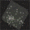 |
Fig. 1 Footprint of the VIS image of the Perseus galaxy cluster covering 0.°84 × 0.°84 and overplotted on the PanSTARRS DR1 g + r + i colour image with FoV ~ 1.°17 × 1.°17; north is up and east left. The green circles show the location of the dwarf galaxy candidates identified in the ERO data, while the grey patches represent the footprint of HST/ACS observations (F850LP/SDSSz, F814w, F791w, F785LP, F775w, F625w, F622w filters). The green circles that fall just outside of the Euclid footprint were identified in an earlier data product with a slightly larger FoV. |
3 Dwarf catalogue and classification
In this section we present the methods used to produce the catalogue of dwarf galaxy candidates in the ERO Perseus field. The detection is carried out visually by inspecting the high-resolution IE image and lower resolution combined IE , JE , and HE colour image. Several steps were taken to clean the list of objects before constructing the final catalogue.
3.1 Visual inspection
Our dwarf galaxy candidates were visually identified by seven contributors using Jafar, an online annotation tool described in detail in Sola et al. (2022). In brief, Jafar displays the images and allows one to navigate around the images, and to zoom in and out. Jafar offers various drawing tools that enable users to precisely delineate the shapes of any objects of interest. To annotate an object, contributors select the most appropriate shape from several options (e.g. ellipse, circle, or polygon), position, resize, and rotate the shape as necessary to trace the contours of the object, and attach a label to classify its type (e.g. ETG, LTG, dwarf galaxy, nucleus, stream, or image artefact). The coordinates of the annotated object are taken from the calculated contours of the drawn shape. All relevant parameters are then stored in an online database. To assist with the classifications, Jafar also has the capability to overlay multiple images and adjust their dynamics, contrast, and brightness.
Upon login, the classifiers were presented with an arcsinh stretched IE image and a combined IE + JE + HE colour image. The high spatial resolution of the VIS image, combined with the arcsinh stretch that enhances the faintest structures, enabled the classifier to identify substructures within the galaxies, for example spiral arms, and hence avoid as much as possible background galaxy contaminants. The presence of any nuclei and/or a large number of GCs was very useful in providing further confirmation of the presence of a dwarf galaxy candidate in the image and sometimes were even used to identify them. Therefore, looking for high concentrations of GCs in the Euclid surveys promises to be a good tool for the detection of GC-rich dwarfs and UDGs.
The colour image was also helpful to distinguish dwarf galaxies from background objects and artefacts. In particular, there are many round ghost halos that resemble dwarf galaxies in the VIS image, but are less prominent in the NIR images and thus appear to have blue colours in the IE + JE + HE colour image.
Dwarf candidates were annotated with ellipses, while potential nuclei were delineated with circles. Examples of such annotations are presented in Fig. 2. Ghost halos were delineated by several contributors with circles and classified as such. All seven classifiers individually inspected the full ERO image, producing seven unique catalogues of candidates with their coordinates, centres, radii, and areas. In total, the classifiers produced 6157 annotations of objects that were flagged as dwarf galaxies.
3.2 Merging the individual catalogues
Before merging the individual catalogues into a single list of unique dwarf candidates, we first crossmatched each catalogue against itself. Ideally, the smallest separation between nearest neighbours amongst all seven catalogues would determine the maximum search radius that could be applied to avoid merging neighbouring dwarfs into a single detection, assuming each catalogue is relatively complete and contains no duplicates. However, this test revealed a small number of objects in almost every catalogue with separations ≲1. A visual inspection of all objects with separations <3 found that 11 objects with the smallest separations were actually nuclei that had been mislabelled as dwarf galaxies, and we also had multiple dwarf-dwarf pairs with a separations ⩾2.6. These nuclei were removed from the sample, and we adopted a search radius of 2″ to retain the dwarfdwarf pairs. The catalogues were then crossmatched using the Astropy (Astropy Collaboration 2013, 2018, 2022) SkyCoords module, generating a list of 2140 dwarf candidates. This number still includes many duplicate objects (40) that were identified in subsequent visual inspections (described below). For this preliminary catalogue, we adopted the average right ascension and declination of the matched objects; the average positional uncertainty for the sample is ±0″.38.
We then investigated the initial agreement between classifiers, as shown in Fig. 3. Care should be taken when interpreting this plot, however. The classifiers were not asked to annotate every object in the image, and therefore, it is unclear how many discrepancies are due to actual disagreements on the classifications of individual objects, and how many objects of interest were simply missed by one or more classifiers. Ideally, the latter case is minimised through the participation of more classifiers, but having more opinions means that it is also difficult to reach full agreement on the classification of any single object. In general, we consider the agreement to be good; 859 objects were flagged as a potential dwarf by a majority (≥4) of the participants, while 264 objects were flagged by all seven classifiers. At the other end, some 876 objects were annotated by a single contributor, and were subsequently removed from further analysis. Most of these are very small objects for which any classification is difficult, background galaxies including lenticulars or spirals, and dwarf irregular galaxies at unknown distances. This cleaning led to an intermediate catalogue of 1260 candidates identified by at least two contributors. To ensure the consistency and robustness of this intermediate list, a final validation step was performed.
The 1260 dwarfs in the intermediate catalogue were validated using an on-line interface. It simultaneously displayed cutouts of the IE and IE + JE + HE colour image, with a fixed FoV 0″.5 across, centred on the object. The same seven contributors re-evaluated the status of each dwarf candidate, assessed their morphology, GC richness, and counted the number of nuclei. The possible responses were: (a) presence of a dwarf, ‘yes’ = 1, ‘unsure’ = 0.5, or ‘no’ = 0; (b) morphology, ‘dE’ – regular early-type galaxy, ‘dI’ – star-forming dwarf irregular galaxy, ‘Disturbed’ – tidally disrupted or interacting object, either dE or dI; (c) number of nuclei, from zero to three; and (d) GC richness, where we define a galaxy as GC-rich if at least two GC candidates were visible within the optical body. A score assessing the presence of a dwarf was computed by taking the mean of all votes from (a).
A consensus list was determined by looking at the histograms of the individual scores. The majority of objects (874) had a score higher than 0.9 and only a few (84) had a score lower than 0.5. To avoid keeping objects that were likely contaminants, we set a threshold at 0.7 (corresponding to a score of 5/7 classifiers), above which the object is securely considered to be a dwarf. This leads to a final catalogue of 1100 dwarf galaxy candidates. Unless explicitly stated, the rest of our analysis is based on these 1100 galaxies. Figure 4 shows examples of dwarf galaxy candidates identified in the ERO Perseus field. Table A.1 summarises the properties of the candidates in our final catalogue, while Table B.1 list the 160 objects with a score lower than 0.7 that were rejected from the final catalogue.
Completeness is not an issue for this study, since we aim to characterise the properties of secure cluster members. Nevertheless, it is important in the context of the analysis of the ERO Perseus cluster luminosity function presented in Cuillandre et al. (2025b). In this paper, it is demonstrated that the completeness begins to rapidly decline at M(IE) = −12, dropping to 50% at −11.
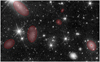 |
Fig. 2 Illustrations of annotated dwarf candidates (red ellipses) and some nuclei (red circles). |
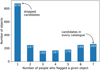 |
Fig. 3 Agreement between the initial catalogues of the seven classifiers. The catalogues were cross-matched within a 2″ radius, and we counted how many people annotated each object as a dwarf galaxy. |
3.3 Morphology, GC richness and nuclei
To determine the final classification of the dwarf candidates, we assigned scores by averaging the number of votes for the morphology (dE/dI, disturbed), GC richness, and presence of any nuclei. Based on the histograms of the scores and a final inspection of the images of each object, we determined the threshold above which the candidate falls into one of the categories. There were generally few cases with scores between 2/7 and 5/7, as most of the histograms were distributed either towards low or high scores or were bimodal around 0 and 1. We set a threshold of two votes out of seven (score = 0.286) to consider the dwarf candidate as a dE, and the same threshold was used to classify it as ‘disturbed’, GC-rich, and nucleated (i.e. the presence of one or more nucleus). This threshold was chosen to include as many galaxies as possible with nuclei, GCs, and signs of tidal disturbances, but that were confirmed by at least two of the seven contributors.
Figure 5 presents the classification break down of the 1100 dwarf candidates in our catalogue. A total of 1061 (96%) are classified as dE (dI: 39 or 4%), 581 (53%) are nucleated, 282 (26%) are GC-rich, and 64 (6%) have a disturbed morphology. Examples of these galaxies are displayed in in Fig. 6, where we show cutouts of select dwarfs classified as: dE, dI, disturbed morphologies, nucleated, GC-rich, or a combination of these features.
4 Comparison with previous dwarf catalogues
A number of studies in the literature have attempted to identify membership in the Perseus cluster, with several studies extending into the dwarf regime (e.g. Brunzendorf & Meusinger 1999; Conselice et al. 2003; Penny et al. 2011, Penny et al. 2014a; Wittmann et al. 2017, 2019; Meusinger et al. 2020; Aguerri et al. 2020; Gannon et al. 2022; Kang et al. 2024). The methods to determine cluster membership differ; some galaxies in these catalogues have been confirmed as members with measured distances, while others are identified as likely members through their morphology and colour.
We first confirmed which galaxies from each source fall within the Euclid ERO image using Multi-Order Coverage (MOC) maps and the Aladin (Bonnarel et al. 2000) ‘filtering by MOC’ feature. MOC maps provide an International Virtual Observatory Alliance (IVOA) standard file format to define arbitrary sky regions (e.g. a FoV) in spherical geometry, using the HEALPix (Górski et al. 2005) tessellation technique; this format allows for the rapid and accurate comparison of two such regions, or regions and catalogues. The filtered catalogues were then cross-matched against our dwarf candidate list, using a 3″.5 search radius, roughly the average effective radius of our dwarf sample (see Sect. 5). It should be noted that the vast majority of our matches have much smaller separations. We summarise the matches between our catalogue and previous surveys in Table 1. Finally, we also cross-matched the literature catalogues against each other to create a master list of unique members.
Three prior surveys attempted to separate cluster members from background objects; Kang et al. (2024) identified cluster members from spectra, Meusinger et al. (2020) present a catalogue of confirmed cluster members as well as galaxies of indeterminate membership, and Wittmann et al. (2019) identified likely cluster members from imaging data. The identification of background galaxies is particularly important because the Perseus cluster, a member of the Perseus-Pisces supercluster, is not truly isolated. Additionally, there are known structures behind the cluster at z ≈ 0.03 and z ≃ 0.06 (see Fig. 8 in Meusinger et al. 2020, and Aguerri et al. 2020) that could be a source of confusion.
Kang et al. (2024) performed a recent spectroscopic survey of objects within 1° of the cluster centre using Hectospec on the 6.5 m MMT. They targeted over 1200 galaxies, selected based on their SDSS magnitudes and supplemented with catalogues from the literature, and estimate that their sample is 67% complete for galaxies with SDSS DR17 apparent r band Petrosian magnitudes rPetro ≤ 18.0. Some 794 of these galaxies fall within the Euclid footprint, of which 212 are confirmed cluster members. Matching our candidate catalogue against all 794 objects, we have 106 galaxies in common: 85 confirmed cluster members and 21 non-members. In Table 1, we further subdivide the galaxies by magnitude, using the rPetro values reported by Kang et al. (2024) for consistency between matched and unmatched objects. To calculate the absolute magnitudes, we adopted a common distance of 72 Mpc for all confirmed cluster members. It should be noted that many of these matches are at the bright end of the dwarf regime, as illustrated in Fig. C.1, and that the two dwarf candidates brighter than Mr,SDSS = −18 are just over the cutoff, with values of −18.0, and −18.32, respectively. Overall, we have good agreement with their catalogue, particularly when one considers that the region between −18 ≲ Mr,SDSS ≲ −16 can be populated by both massive and dwarf galaxies (Dunn 2010), and the Kang et al. sample is not exclusively a dwarf sample.
The 21 non-cluster member matches in our catalogue warrant additional scrutiny. We find: two were flagged as point sources and thus are bad matches; one has a negative redshift so we cannot assign a distance with confidence; two foreground objects fall just outside the caustics used to define the cluster; eight have redshifts between 0.026 and 0.030 and are likely associated with background structures; and the remaining eight galaxies all have measured redshifts 0.07 ≤ z ≤ 1.25. None of these galaxies were flagged as having poor spectra, but if all of the measurements are accurate, the candidates at the largest distances would have unphysically large radii and absolute magnitudes as bright as the brightest galaxies in the Perseus cluster, despite their low surface brightnesses. Thus, we suggest taking the high redshift values with caution. Conversely, the lower redshift galaxies appear plausible, and eight galaxies (the two foreground galaxies and six in the range 0.026 < z < 0.030) have absolute magnitudes Mr,SDSS > −18, which would explain our difficulty in separating them from dwarf galaxies within the Perseus cluster. These numbers suggest an accurate rate of 80–90% for our catalogue, depending on the weight that is given to the point sources and high-redshift galaxies. It should be noted that these galaxies have not been removed from our sample of 1100 dwarf candidates.
The Kang et al. (2024) catalogue can be further used to check for dwarf cluster members that we missed or rejected. There are 27 confirmed cluster members with Mr,SDSS > −18 that are not in our catalogue. These galaxies are typically at the bright end of the dwarf magnitude range, with the majority (26) having absolute magnitudes between Mr,SDSS = −18 and −16. This interval is populated by both dwarf and non-dwarf galaxies (e.g. low surface brightness spirals and compact ellipticals), and therefore it is not surprising that we have some level of disagreement. Finally, we also matched our intermediate catalogue against the Kang et al. (2024) sample to check if any of the candidates that were removed from the sample due to low confidence scores have redshifts; only one such galaxy has a match, and it is a confirmed background galaxy with a redshift z = 0.026658.
Although not a spectroscopic survey, the Wittmann et al. (2019) sample is another important comparison for this work. They present a study of the Perseus cluster much like this one, using morphologies and colour to separate potential cluster members from background galaxies, with a catalogue containing 5437 galaxies in the direction of the Perseus cluster core. Nearly all of these galaxies fall within the Euclid ERO FoV. Wittmann et al. (2019) visually classified each galaxy into one of eight categories: dE/ETG cluster members, candidate cluster members, background ETGs, LTGs, edge-on disk galaxies, galaxies with weak substructure, merging background galaxies, and excluded sources (e.g. image artefacts or Galactic cirrus). For this comparison, we adopt the Wittmann et al. nomenclature, where the first two categories are considered candidate cluster members. They did not attempt to separate cluster and background LTGs, disk galaxies, or galaxies with weak substructure; for simplicity, we have merged these with the remaining categories – aside from the excluded sources – and collectively refer to them as non-cluster members. After matching the catalogues, we find 389 cluster members in common between our samples (348 ‘dE/ETG cluster candidates’ and 41 ‘candidate cluster members’). In Table 1, we break down the number of proposed cluster members in two magnitude bins using the MV magnitudes from Wittmann et al. (2019): massive galaxies with MV ≤ −18 and a dwarf sample (MV > −18). Only one of our dwarf candidates falls in the massive galaxy bin, and it has MV = −18.1, placing it right on the cusp of the separation. Among the dwarf candidates, our agreement is ≳80%. Interestingly, this is also the typical level of agreement between the seven classifiers in this work with each other (80–90%), and may reflect inherent biases in the selection of dwarf galaxies that translate into differences between catalogues.
Only 37 of the proposed Euclid dwarf members were labelled as non-cluster objects (18 background ETGs, 7 LTGs, 7 edge-on disk galaxies, and 5 galaxies with weak substructures) in the Wittmann et al. (2019) sample; none of our galaxies matched with objects identified as cirrus or image artefacts in their sample. However, Wittmann et al. note a few caveats in the classifications: small sources that could not be readily classified given the resolution of the WHT were classified as background ETGs, some of the LTGs may be legitimate cluster members, and the classification of galaxies with weak substructures is ambiguous. Thus, it is entirely possible that our matched objects are legitimate cluster members, although distance estimates will be required to prove or disprove their membership. In the region of overlap between the two surveys, we identify an additional 143 dwarf candidates with no matching Wittmann et al. sources (cluster member, non-cluster member, or excluded source) within 3″.5. These galaxies have a range of magnitudes, surface brightnesses, and sizes, as visualised in Fig. C.3, but they are more concentrated among our fainter and smaller candidates, which is a likely a result of the increased depth of Euclid.
The Meusinger et al. (2020) catalogue includes 1294 galaxies in a 10 deg2 field around the cluster, which can be separated into confirmed cluster members, confirmed non-members, and a number of galaxies that are still lacking distance estimates. The confirmed cluster members have spectroscopic redshifts taken from various sources (SDSS, TLS Tautenburg telescope, CAHA telescope at Calar Alto Observatory, NED, and Hα data from Sakai et al. 2012 and Moss & Whittle 2000, 2005), and were also included in the Kang et al. (2024) sample discussed above. For completeness, we perform our own comparison using the full Meusinger et al. (2020) sample here. Only 213 of the 1294 galaxies fall within the Euclid ERO FoV: 116 cluster members, 3 non-members, and 94 unconfirmed galaxies. Each of these populations can be further subdivided into dwarf and non-dwarf categories. To be as complete as possible, we cut the sample based on either the reported stellar mass estimates log10 M*/M⊙ ≤ 9.0, or Mr,SDSS > −18, where the absolute magnitude was calculated assuming the distance to the cluster of 72 Mpc. As seen in Table 1 and Fig. C.2, the Meusinger et al. sample is skewed towards massive (brighter) galaxies. Of the 12 dwarf cluster members in their catalogue, we identified six. A visual inspection of the six galaxies we missed revealed that one is a spiral, and the other five have noticeably steeper light profiles, such that they may be better classified as compact ellipticals. If we assume that the unconfirmed galaxies are also cluster members, then 86 of the galaxies in the subsample would be dwarf candidates and we match 51 of these (∼60%). It should be emphasised that these galaxies are likely a mixture of members and non-cluster members, however, and thus one would not expect an overly strong agreement.
In addition to the large surveys discussed above, smaller, targeted studies have obtained distances measurements to a select number of other galaxies in the Perseus cluster. Penny et al. (2014a) have Keck-ESI spectra of six dEs in the cluster core, while Gannon et al. (2022) obtained integral field spectroscopy of three UDG candidates in the Euclid FoV with the Keck Cosmic Web Imager (KCWI; Morrissey et al. 2018). Four of the galaxies from Penny et al. (2014a) are in our sample; the other two are badly contaminated by intracluster light in the core, and were not flagged during our initial inspection of the images. In the case of Gannon et al. (2022), we identified all of the UDGs in the Euclid FoV.
The Gannon et al. (2022) galaxies were taken from the larger sample of UDG candidates in Wittmann et al. (2017). The Wittmann et al. (2017) catalogue contains 89 UDG candidates, and is particularly useful for testing our completeness at the faint end of the luminosity function. Of the 89 galaxies in their sample, 85 are in the Euclid FoV and we match 72 candidates with our catalogue. Li et al. (2022) also built upon the Wittmann et al. sample, further identifying 10 of the UDG candidates based on overdensities in the intergalactic GC population, as identified in the HST PIPER survey; nine of these UDGs are in our sample. In addition to the known UDGs, Li et al. (2022) found an interesting object that they designated CDG-1, a potential galaxy with an overdensity of GCs but no detected diffuse stellar content. The GCs are all found in the Euclid GC catalogue (see Sect. 6.5) but we do not find any diffuse emission at this location. The most likely scenario is that this is a random grouping of objects that is not associated with a galaxy.
At another extreme, Penny et al. (2012) identified 84 ultra compact dwarf (UCD) candidates in the Perseus cluster core, and Penny et al. (2014b) spectroscopically confirmed 14 as members of the cluster. None of these galaxies – neither the confirmed UCD cluster members nor the UCD candidates – are in our sample. This is unsurprising, however, as their small sizes and relatively high surface brightnesses would have precluded their selection during the visual examination of the images.
In total, 494 of the dwarfs in our sample have already been identified in previous studies. The remaining 606 galaxies appear to be new detections.
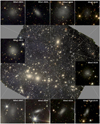 |
Fig. 4 VIS-NISP colour image of the Perseus galaxy cluster. The full FoV of 0.°84 × 0.°84 is shown; north is up and east is to the left. Examples of dwarf galaxy candidates are shown in the individual cutouts of size 40″ × 40″. The galaxies EDwC-0854, EDwC-0468, EDwC-0165, and EDwC- 0997 are newly identified UDG candidates. The system composed of EDwC-0141 and EDwC-0145 (bottom right cutout) shows one example of two newly identified dwarfs that appear to be interacting. |
 |
Fig. 5 Classification of the final catalogue of 1100 dwarf galaxy candidates. The darker shades on the outer circle correspond to the presence of the feature of interest. Left: nucleated fraction (outer circle) as a function of morphology (inner circle). Middle left: GC richness (outer circle) as a function of morphology (inner circle). Middle right: signs of disturbed morphology (outer circle) as a function of morphology (inner circle). Right: GC richness (outer circle) as a function of the nucleated fraction. A total of 1061 (96%) dwarf galaxy candidates are classified as dE (dI: 39 or 4%), 581 (53%) are nucleated, 282 (26%) are GC-rich, and 64 (6%) have a disturbed morphology. |
Previous surveys of the Perseus cluster that extend into the dwarf regime.
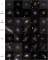 |
Fig. 6 Cutouts of some dwarf candidates, taken from the VIS-NISP colour image created using the IE band in blue, the YE band in green, and the HE band in red. The colours are projected onto the high-resolution IE band to best reflect their appearance as detected. From top to bottom: dE; nucleated dE; GC-rich dE; disturbed morphologies; multiple nuclei; dI; and GC-rich dI. The sizes of the cutouts are proportional to twice the area determined from the annotation of classifiers; north is up and east is to the left. |
5 Photometry and structural parameters
5.1 Extinction correction
To derive the correct values of the attenuation due to the Milky Way (MW) dust the following ingredients are needed: the map of the Galactic dust distribution; an extinction law; the spectral energy distribution (SED) of the extragalactic source; and the transmission functions of the relevant filters.
The sky region of the Perseus cluster is significantly affected by extinction from MW dust, as can be seen in Fig. 7. To correct for it, we adopted the HEALPix (Górski et al. 2005) dust opacity map with Nside = 2048 released by the Planck Collaboration in 2013 (Planck Collaboration XI 2014)2. This map provides information on the colour excess E(B − V) - obtained with data from which point sources were removed –, the optical depth at 353 GHz τ, and its uncertainty dτ. Each galaxy was associated with the HEALPix pixel containing its coordinates, from which we derived the values of E(B − V) and its uncertainty dE(B − V) = E(B − V) dτ/τ.
To derive the attenuation at different wavelengths we used the extinction curve k(λ) = RV × A(λ)/AV, where A(λ) and AV are the magnitudes attenuated at the wavelength λ and in the V filter, from Gordon et al. (2023), with RV = 3.1 implemented through the dust-extinction package3.
The correct derivation of the attenuation in each observed bandpass depends on the SED of each object (e.g. Galametz et al. 2017). However, since the SED of each galaxy is unknown, a general approach is to assume a test case SED, e.g. a flat spectrum in frequency or a stellar SED. We employed the flux F from a 5700 K blackbody, to represent a G7V star, which resembles a typical galaxy continuum, as a proxy.
Finally, the exact attenuation in each band, especially in the broad bands that we are considering in the present work, depends also on the shape of the throughput, including filter, optics, mirror, and detector. We used the official bandpasses R(λ) for NISP (Euclid Collaboration: Schirmer et al. 2022)4 and VIS (Cropper et al. 2016; Euclid Collaboration: Scaramella et al. 2022).
With the above ingredients, for each filter x we derive the quantity cx as
 (1)
(1)
which can be used to obtain the intrinsic magnitudes as mobs − cxE(B − V). With this approach, we obtained cx = 2.122, 1.066, 0.726, and 0.470 in the IE, YE, JE, and HE bands, respectively.
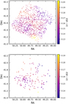 |
Fig. 7 Map of the colour excess E(B − V) for the dwarf galaxy sample (top) and the bright galaxy sample (bottom) presented in Cuillandre et al. (2025b). |
5.2 Cutouts
The cutouts for the photometric and structural parameter analysis were generated with sizes of 9 Re (Poulain et al. 2021), where the preliminary estimate of Re was determined by using the area in deg2 defined by the users with the annotation tool and assuming a visual extent of the galaxy corresponding to approximately 2Re.
Of the 1100 dwarf cutouts, 16 had to be recut to a smaller than 9 Re size as they fall near the edge of the image, which caused issues with the fitting algorithms. For these galaxies, we created smaller cutouts while making sure to have sufficient remaining sky level pixels in the image. Because a number of galaxies (24) fall outside the FoV of the ERO Perseus observations in one or more Euclid NIR filters, the measurements for those galaxies were not possible and therefore the tables of photometric parameters show no entries for that particular galaxy and filter.
The cutouts were created with the same angular size for all IE as well as YE , JE , and HE images. The range of cutout regions provided from the annotation tool corresponds to 10″–170″ (or 5 kpc–60 kpc).
The masking of contaminating sources in the cutouts is done via two main steps. The first step is to run MTObjects (Teeninga et al. 2015) that produces the MTO segmentation image. The advantage of using MTObjects is that it is capable of locating the faint outskirts of objects. The code is run for all the IE and YE, JE , and HE image cutouts independently. In order to avoid including the dwarf galaxy in the mask, the parameter move_factor is optimally selected for the ERO Perseus images and furthermore, a region of size 1 Re, centred on the dwarf galaxy, is unmasked after this step is completed. The masks are also visually inspected. The second step involves running SExtractor (Bertin & Arnouts 1996), which is good at detecting faint point sources – including within the galaxy of interest – on all of the IE and YE, JE, and HE image cutouts. We run SExtractor three times with different regions of the image centred on the dwarf masked, as well as different detection and analysis thresholds, minimum and maximum areas, background mesh sizes and deblending contrasts.
The MTO and SExtractor masks are then combined to create a final mask. To ensure that the nucleus of the dwarf has been masked by the SExtractor runs, the nucleus of each of the nucleated dwarfs identified by our visual inspection is masked in a final step. The exact position of the nucleus is determined by finding the maximum pixel value within a region of 15 pixels around the galaxy coordinates and a region of 4(2) pixels in radius in the IE (YE,JE,HE) images is masked in order to make sure that the nucleus does not affect the fit of the diffuse component of the dwarf galaxy.
5.3 Photometric and structural parameters
The galaxy modelling was first performed on the IE images due to the better spatial sampling and spatial resolution. We first applied a non-parametric galaxy image analysis method to obtain an initial guess of the structural parameters of each dwarf galaxy using AutoProf (Stone et al. 2021). The masks were used, but since complete isophotes cannot be masked using AutoProf (it ignores the mask in this case), the nuclei were not masked in this first step. A total of 872 sources finished with convergence and 228 did not converge. The following photometric and structural parameters were calculated from the AutoProf output: total magnitude (IE); effective radius (Re); surface brightness (central:  , at
, at  , and within
  ; Sérsic index (n); position angle (PA); and axis ratio (AR). For the galaxies with no convergence, we used the median value of the results from the fits that finished with convergence for the next step (see below).
These initial estimates of the structural parameters were then used as inputs to both Galfit (Peng et al. 2010) and AstroPhot (Stone et al. 2023). The model used for both consists of a twodimensional (2D) Sérsic function (Sérsic 1963) combined with a PSF.
To obtain the PSF models, we first used SExtractor to detect high S/N sources (DETECT_MINAREA = 5; DETECT_THRESH = 100 for IE and DETECT_THRESH = 40 for NISP). Then, point sources were selected and PSF models were created with PSFEx (Bertin 2011) using the pixel basis, PSFVAR_DEGREES = 2, and without oversampling or undersampling. The PSF models at the centres of the images were reconstructed from the PSFEx output as a linear combination of the PSF vectors. The PSF models for IE, JE, YE, and HE are shown in Fig. 8.
The Galfit and AstroPhot codes were run in parametric mode using the above model and masks. In addition, two runs of AstroPhot were performed using different sky models, a flat and a plane sky model. The plane sky model was run in order to improve the fitting outcome of the dwarfs embedded in strong sky gradients due to a nearby massive (bright) galaxy. All models and residuals produced by both codes were visually inspected and the output parameters of the best fits were retained for the final catalogue.
From these runs, a total of 854 dwarf galaxies returned a good fit and therefore robust structural parameters. The remaining 246 galaxies required manual intervention. For 123 dwarfs, it was necessary to manually edit the masks due to bright stars or other sources of contamination that fell within the central 1 Re of the dwarf, a region that was previously unmasked in MTO in order to avoid removing the dwarf itself. For the remaining 123 galaxies, patching of the image was needed because adjusting the masks was not enough. These cases were extreme and showed very strong contamination from stellar spikes, stars, bright nearby galaxies, or a combination of features. Of these, the smaller (and faint) dwarfs were the most affected and difficult to fit. These 89 dwarf galaxies have a Sérsic index of 0.36 or below. For n < 0.36 the meaning of Re and IE changes (Sérsic 1963); they are no longer at the half light radius. AstroPhot uses the fourth-order expansion of bn (Sérsic 1963) to get down to n = 0.36, but higher orders are needed to go further. Therefore, for the dwarfs with n ≤ 0.36, the extracted parameters should be treated with caution and with this limit in mind. We note that some of those galaxies actually have a good fit from Galfit, so this caution does not apply to all 89 dwarfs.
Histograms of the extracted parameters are shown in Fig. 9 and the values for each dwarf candidates are given in Table A.2. The absolute magnitudes and effective radii (in kpc) were computed using the distance of 72 Mpc.
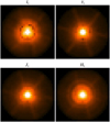 |
Fig. 8 PSF models with the native pixel scale of IE , YE , JE, and HE in the centre of the ERO Perseus images. The displayed PSF models have a sidelength of 3″.1 for IE and 9″.3 for YE, JE, and HE. The models are displayed in logarithmic scale. |
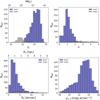 |
Fig. 9 Photometric and structural parameters derived from the surface profile fitting of the 1100 dwarf galaxy candidates and the bright galaxy sample from Cuillandre et al. (2025b) in the ERO Perseus field shown in violet and light grey, respectively. All magnitudes and surface brightness values were corrected for extinction, as described in Sect. 5.1. |
5.4 Colours
Once the photometry and structural parameters of the dwarfs were obtained, aperture photometry was performed on all VIS+NIR images to obtain colour information on the dwarfs. The aperture photometry was done using the python package photutils and using a circular aperture of 1 Re, with the effective radius taken from the best fit to the dwarf in the IE image. The aperture photometry was performed without using a mask and hence includes any nucleus or contaminating source. The aperture magnitudes were then corrected for extinction using the method described in Sect. 5.1 and applied at each dwarf position independently and for each Euclid passband.
5.5 Masking
The aperture photometry magnitudes, the extinction correction (EC) at each galaxy position and Euclid passband, and the level of contamination from other sources within the aperture are given in Table A.3. The distribution of VIS-NISP aperture colours of the Perseus dwarfs are shown in Fig. 10. We compare these colours with those of the three dwarf irregular galaxies IC 10, Holmberg II, and NGC 6822 presented in Hunt et al. (2025). We find that their reported IE − HE colours of −0.419 ± 0.105, 0.029 ± 0.090, and 0.250 ± 0.059, respectively, fall well within the colour distribution shown in Fig. 10 for the ERO Perseus dwarfs. The NISP-NISP aperture colours were also computed and can be found in Fig. D.1.
6 Results
6.1 Luminosity and stellar mass function
The luminosity and stellar mass function (LF and SMF, respectively) of the ERO Perseus galaxy population, consisting mostly of the dwarf galaxy sample presented here, is discussed in a separate paper (Cuillandre et al. 2025b). The faint end slope of the LF, αS, is found to have a value of αS = −1.2 to −1.3. The criteria used to identify all cluster members, maximise completeness and minimise the contamination of foreground and background sources, along with the interpretation of the results in terms of models, can be found in Cuillandre et al. (2025b).
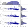 |
Fig. 10 Euclid VIS-NISP colours as a function of IE measured using aperture photometry within 1 Re of the 1100 dwarf galaxy candidates and the bright galaxy sample in the ERO Perseus field from Cuillandre et al. (2025b) shown in violet and light grey, respectively. The magnitudes were corrected for extinction before the colours were computed, as described in Sect. 5.1. |
6.2 Scaling relations
Galaxy populations can be characterised in structural parameter spaces (see e.g. Kormendy 1985; Bender et al. 1992; Binggeli 1994; Kormendy et al. 2009). In order to compare the structural parameters of our dwarf galaxy sample to scaling relations in the literature, we have to convert the IE magnitudes and surface brightnesses to the V band. To select the UDGs in our sample, we have to convert them to the g band.
The magnitude transformation from IE to V band is derived using synthetic photometry of SEDs of old stellar populations with subsolar metallicities, about [Fe/H] = −0.5 (Saifollahi et al. 2025), similar to quiescent dwarf galaxies in cluster environments: V = IE + 0.5. The transformation from the V band to the SDSS g band is taken from Lupton (2005)5: g = V + 0.31.
We select UDGs based on the definition of van Dokkum et al. (2015), i.e. µg,0 ≥ 24 mag arcsec−2 and Re ≥ 1.5 kpc. This selection cut yields 93 UDGs for our 1100 sample of dwarf galaxies with structural parameters. This corresponds to 8.5% of our total dwarf sample, compared to a smaller fraction of 2.7% in the Mass Assembly of early Type gaLAxies with their fine Structures (MATLAS) survey (Marleau et al. 2021) and 5.4% reported by Zöller et al. (2024) for A262 and A1656. The VIS cutouts of the Perseus UDGs are shown in Fig. 11.
The higher fraction of UDGs in our sample is likely due to the greater surface brightness depth of the ERO data (by 0.5–1 mag when comparing to the MATLAS survey) and the high angular resolution of the Euclid data that enables one to clearly distinguish faint dwarfs/UDGs from background sources. The four UDGs in our sample with the lowest central surface brightness are EDwC-0035, EDwC-0424, EDwC-0926, and EDwC- 0932 ( mag arcsec−2). We note that other dwarf candidates that are not classified as UDGs have even fainter surface brightness, with the faintest, as measured at Re , being the dwarf candidate EDwC-0239 with
  mag arcsec−2 (not extinction corrected).
We investigate which regions the dwarf galaxies in our sample populate in the MV−Re,  , and
, and  parameter spaces and compare them to scaling relations from the literature in Fig. 12. The structural parameters of ellipticals are taken from Bender et al. (1992) and Kormendy et al. (2009), while those of classical bulges are from Fisher & Drory (2008), Kormendy et al. (2009), and Kormendy & Bender (2012). The structural parameters of BCGs are from Kluge et al. (2020). The literature data points of dwarf galaxies contain Local Group dwarf spheroidals from Mateo (1998) and McConnachie & Irwin (2006), Virgo dwarf spheroidals from Ferrarese et al. (2006), Gavazzi et al. (2005), and Kormendy et al. (2009), dwarf galaxies (including UDGs) from the MATLAS survey (Poulain et al. 2021; Marleau et al. 2021), and dwarf spheroidals (including UDGs) in A262 and A1656 (Coma cluster) from Zöller et al. (2024). Within the dataset from the literature, BCGs, ellipticals, and classical bulges are represented in dark grey, and dwarf galaxies (including UDGs) are represented in light grey. Bright galaxies from the ERO Perseus luminosity function project Cuillandre et al. (2025b) are depicted in black. Our dwarf sample is split up into UDGs (orange) and non-UDGs (violet).
The majority of our data points follow the scaling relations of dwarf galaxies from the literature. In the  and
and  parameter spaces, the dwarf distribution is slightly extended towards fainter μV,e. Furthermore, the diffuse end of the dwarf parameter relations are more densely populated than in previous studies. This indicates higher completeness of diffuse galaxies, presumably due to a combination of the high depth and high spatial resolution delivered by Euclid that provides a better separation from contaminating objects. The increased density within the diffuse part of the parameter spaces is particularly evident in the
  relation, which significantly deviates from the scaling relations reported in Kormendy et al. (2009). In that paper, a narrow
  scaling relation is reported for the dwarf spheroidals, whereas the distribution of our dwarf galaxy sample is nearly twice as broad. When comparing with datasets from more recent dwarf surveys, such as the MATLAS survey (Marleau et al. 2021), the Next Generation Virgo cluster Survey (NGVS; Ferrarese et al. 2012) and the Next Generation Fornax Survey (NGFS; Muñoz et al. 2015), we find good agreement with the spread of the distributions. Examples of galaxies with structural parameters similar to the most extreme galaxies found in this study were also reported by Zöller et al. (2024). We also find a few galaxies above the
  and
and  or below the MV− Re scaling relations of dwarf galaxies; we cannot exclude the possibility that these could be interloping background galaxies.
Furthermore, we note that while UDGs populate the diffuse extension with respect to the scaling relations of spheroidals from Kormendy et al. (2009), there are also some galaxies populating those regions that do not fulfil the UDG definition. We conclude that the UDG definition does not cover all of the most extreme diffuse galaxies with respect to these structural parameter relations, which is in agreement with the findings from Marleau et al. (2021) and Zöller et al. (2024).
As the UDG definition is not unique in the literature, we also examine the size of our UDG sample given the definition of Lim et al. (2020), based on deviations from the galaxy scaling relations. They define their primary sample of UDGs to be those systems that deviate towards large size or low surface brightness by more than 2.5σ (selected based on a possible gap seen close to 2.5σ from the mean relation) in each of the three scaling relations: MV−Re,  , and
, and  . They also define a secondary sample of UDGs that deviate by at least 2.5σ in only one or two of the scaling relations. The combination of the primary and secondary samples is then said to be of high completeness. Using the same approach, we compute a total of 32 UDGs (38 UDGs if we calculate 2.5σ from the median instead of the mean), with none of them being in the primary sample. We note however that this selection method is highly dependent on the scatter (measured by the standard deviation σ) of the scaling relations for a given sample as well as the putative presence of a gap at 2.5σ, which we do not see in our scaling relations.
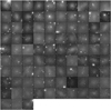 |
Fig. 11 Cutouts of the VIS image for the 93 UDGs in the ERO Perseus field, comprising 8% of the dwarf sample. The UDGs were selected to have an effective radius Re ≥ 1.5 kpc and a central surface brightness in the g band µg,0 ≥ 24 mag arcsec−2. The sizes of the cutouts are proportional to twice the area determined from the annotation of classifiers; north is up and east is to the left. The UDGs are ordered by decreasing surface brightness |

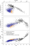 |
Fig. 12 Comparison between MV, Re, and μV,e scaling relations of the ERO Perseus dwarf sample (violet), including UDGs (orange) from this work, and bright galaxies (black) from Cuillandre et al. (2025b). The basis for this plot is Figure 37 in Kormendy et al. (2009) with updates from Kormendy & Bender (2012), Bender et al. (2015), Kluge et al. (2020), Marleau et al. (2021), and Zöller et al. (2024), including brightest cluster galaxies (BCGs), ellipticals, and classical bulges (dark grey), as well as dwarf galaxies including UDGs (light grey). For the sake of clarity, we do not show the errorbars. The uncertainties vary significantly between the different galaxies. |
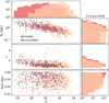 |
Fig. 13 Scaling relations of IE as a function of Re (top), Sérsic index n (middle), and axis ratio (bottom) of the nucleated (pink) and nonnucleated (peach) dEs in the ERO Perseus field. We display the distribution of magnitude for the whole samples, and of the Re, n, and the axis ratio within the same magnitude range 17.3 ≤ IE < 23.6. |
Fraction of nucleated dwarfs as a function of the magnitude and morphology of the host dwarf.
6.3 Nucleated dwarf properties
The morphological classification of the dwarfs led to a sample of 582 nucleated galaxies, comprising 52.9% of the dwarf sample. A thorough analysis of the effect of the galaxy luminosity and the environment on the nucleated fraction will be presented elsewhere (Euclid Collaboration: Sánchez-Janssen, et al., in prep.). We study as a first step the dependence of the nucleated fraction on the luminosity and morphology of the dwarfs. In Table 2, we report the nucleated fraction for the whole sample, as well as for the subpopulations of dEs and dIs. We divide the samples into two bins, namely faint and bright dwarfs, by cutting at the mean apparent magnitude of the sample IE = 20.4 [corresponding to M(IE) = −13.9]. Studies across a wide range of environments have reported that nucleated dwarfs tend to be brighter than nonnucleated dwarfs, regardless of the morphological type, such that brighter dwarfs have higher nucleated fractions (e.g. Côté et al. 2006; Ordenes-Briceño et al. 2018; Sánchez-Janssen et al. 2019a; Habas et al. 2020; Hoyer et al. 2021; Zanatta et al. 2021; Carlsten et al. 2022). In agreement with the literature, we find a higher nucleated fraction for the bright dwarfs as compared to the faint ones, with 81.3% (8.3%) of the bright dEs (dIs) being nucleated, against 32.5% of the faint dEs and none of the faint dIs. We find overall a larger nucleation fraction for the dEs as compared to the dIs, which is consistent with the observations of Habas et al. (2020), but different from the expectations from Neumayer et al. (2020), where the fraction of nucleated dEs and dIs are similar. The difference between the two fractions can be explained by the low statistics of the dI sample, with two of the 39 galaxies being nucleated, but also from the fact that it is more difficult to identify nuclei in irregular galaxies due to the presence of star-forming regions and dust obscuration.
As a second step, we investigate possible differences between the structural properties of the nucleated and non-nucleated dwarfs. Recent results strongly indicate that nuclear star clusters (NSCs) in low-mass galaxies grow primarily via dissipationless merging of pre-existing massive star clusters (e.g. Turner et al. 2012; Sánchez-Janssen et al. 2019a; Fahrion et al. 2022). In this scenario, it is expected that the structural parameters of the host galaxy play a relevant role in both setting the efficiency of dynamical friction and the strength of the cluster mass loss as it spirals inward (Leaman & van de Ven 2022). For example, den Brok et al. (2014) find that Coma dwarfs that are more concentrated and rounder tend to host more luminous star clusters. In addition, it has been shown that nucleated cluster dwarfs are intrinsically rounder, at all luminosities, than their non-nucleated counterparts (Sánchez-Janssen et al. 2019b; Lisker et al. 2007; Venhola et al. 2019).
In Fig. 13, we show the scaling relations between IE and the effective radius Re , the Sérsic index n, and the axis ratio of the nucleated and non-nucleated dwarfs in Perseus. Given the low statistics of the dI sample, we focus here on the dEs only. For each relation, we also include histograms of the property distributions within the same magnitude range 17.3 ≤ IE < 23.6. We limit the range of Sérsic index values to n ≥ 0.5 because smaller values indicate a 3D luminosity distribution that is deficient at the centre, which is unphysical (Trujillo et al. 2001). From the distributions of IE , we see that the nucleated dwarfs tend to be brighter than the non-nucleated ones. Looking at the structural properties at similar magnitudes, we observe similar ranges of properties. However, the distributions do not peak at the same value, such that the nucleated distributions are shifted towards larger Re , n, and higher axis ratios. This means that we observe fewer nuclei in smaller, high-ellipticity dwarfs, as well as in galaxies with flatter surface brightness profiles. These results are consistent with the observations in other galaxy clusters and lower density environments (e.g. Sánchez-Janssen et al. 2019a; Neumayer et al. 2020; Poulain et al. 2021).
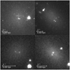 |
Fig. 14 Examples of dwarfs that stand out due to the number of their nuclei candidates. |
6.4 Dwarf nucleated substructures
During the visual review of the dwarf candidates, the classifiers were allowed to identify multiple nuclei in the dwarfs. A galaxy is visually defined as multinucleated when at least two compact sources of similar luminosity are located close to the photometric centre and are brighter than other surrounding compact sources. The presence of multiple nuclei can be linked to dwarf-dwarf mergers (Pak et al. 2016), where the NSCs of both interacting galaxies are migrating towards the potential well of the newly formed galaxy. Another possibility is the observation of a nucleus with a stellar disc, similar to the double nucleus of M31 (Lauer et al. 1993). Given that the dwarf nuclei can have similar photometric and structural properties to massive GCs (e.g. Poulain et al. 2021; Hoyer et al. 2023), we can also be observing the infall of massive GCs towards the galaxy centre due to dynamical friction (Lotz et al. 2001). Finally, we cannot exclude the possibility that in some cases, the candidate nucleus or nuclei might be a background galaxy or foreground star, seen in projection on top of the galaxy. We show in Fig. 14 examples of four multinucleated dwarfs.
Together with multiple nuclei, reviewers also noted the presence of complex nuclei in a few tens of objects. These NSCs exhibit some tidal features such as stellar tails, suggesting an ongoing interaction at the centres of the galaxies. These types of structures can be identified only with the depth and high spatial resolution of the VIS observations, since such structures are not resolved in the other bands. Four such nuclei with complex structure are visible in Fig. 15. Further investigations are needed to assess the nature of these substructures, which is beyond the scope of this paper.
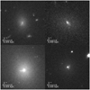 |
Fig. 15 Examples of dwarfs that stand out due to the presence of a complex nucleus. |
6.5 Globular clusters
To investigate the GC population in galaxies within our field, we adopted two distinct approaches. First, we examined galaxies visually identified as GC-rich, comparing their properties (such as position in the cluster, Sérsic parameters, etc.) with those of GC-poor galaxies in the sample. Then, we adopted a more quantitative approach to estimate the total GC population in each galaxy, and inspected the overall characteristics of the GC systems within these galaxies. Showing the results for both visual and automatic detection methods for GC-rich dwarfs serves two key purposes: maintaining coherence with other sections, which rely on visual inspection, and providing validation for the visual approach.
6.5.1 GC richness from visual inspection
As described in Sect. 3.3, during the visual inspection of dwarf galaxies in the Perseus field, classifiers were asked to verify the presence of GC candidates hosted within the galaxies. GC candidates were visually identified as relatively compact and faint sources with a surface distribution centrally concentrated around the galaxy. In this context, a dwarf galaxy was categorised as GC-rich if it contained a minimum of two GC candidates. Part of the reason we chose this low value was to separate the dwarfs with potential GC candidates from the vast majority of dwarfs with zero (±1) GC candidates.
With this (somewhat arbitrary) definition of GC richness in mind, Fig. 16 compares the spatial, photometric and structural properties of visually GC-rich galaxies with those of the non- GC-rich elements in the catalogue. For the sake of clarity, only dwarfs with GC scores ≥ 0.85 are indicated, corresponding to those receiving 6 votes out of 7.
One possible source of confusion in visually inspecting GC richness could arise from the proximity, at least in projection, of a dwarf candidate to a bright, massive companion or to regions of high intracluster GC population density (Kluge et al. 2025). Figure 16 (upper left panel) shows the positions of dwarf and bright galaxies in the Perseus field. Here, grey filled circles represent galaxies brighter than IE = 16 [absolute M(IE) = –18.3], with symbol size scaled with the galaxy effective radius. The full sample of dwarf galaxies is reported with violet dots. GC- rich candidates are denoted by filled or empty orange circles. Filled orange symbols are assigned to dwarfs projected far from any bright galaxy, while empty orange circles are used for dwarfs within 5 effective radii of a bright companion.
A first observation is the absence of any obvious GC richness enhancement near the bright (massive) galaxies in the field. This suggests a real overdensity of GCs associated with the dwarfs rather than contamination from the intracluster GCs or the GC system of a nearby massive companion. Furthermore, we do not observe significant evidence of any other trends apart from the clustering of dwarfs around the massive galaxies. Indeed, a clear east–west stretch is evident both for the dwarfs and the giant galaxies.
The remaining panels of Fig. 16 show the properties of the dwarf galaxy sample, using the same colour and symbol coding as in the upper left panel, except for the bright galaxies which are not shown. By considering as ‘consensus sample’ the dwarfs with at least 6 out of 7 votes in favour of GC richness, in Fig. 16 we observe the following.
- –
No GC-rich and uncontaminated candidate has Re < 2.″0 (~800 pc) or is fainter than IE ~22 (lower left panel).
- –
Two GC-rich objects exhibit IE ≳ 21 [fainter than the absolute magnitude M(IE)~ –13.3]. One of them is located near the denser cluster area, close to the cluster core, suggesting the possibility of intracluster GCs or bright galaxy GC contamination. The other dwarf (EDwC-0066) appears as a faint diffuse object with a handful of point-like sources within one effective radius (lower left panel).
- –
Within fixed IE intervals, and for galaxies brighter than IE ~ 20, the GC-rich candidates appear to have, on average, slightly smaller n values compared to the GC-poor sample. This trend appears to be weak but consistent over the range of 16 ≤ IE ≤ 20. For example, in the 18–19 magnitude bin, we find 〈n〉 = 1.0 ± 0.1 for the 19 GC-rich dwarfs, compared to 〈n〉 = 1.4 ± 0.3 for the 28 GC-poor dwarfs (only including those with a score ≤ 1 out of 7 votes; lower middle panel).
- –
For IE ≤ 20, there appears to be a tendency for the central surface brightness of GC-rich dwarfs to be slightly fainter than that of the entire sample of dwarfs in the same magnitude range (lower right panel).
- –
The Sérsic exponent, n, shows a correlation with the host galaxy central surface brightness. This behaviour has been previously observed (e.g. Ferrarese et al. 2006); here, we find that it appears to be independent of the GC richness (upper middle panel).
- –
Approximately 40 GC-rich uncontaminated dwarfs (orange filled circles in the figure) have Re ≥ 1.5 kpc; among them, about ten have central surface brightness
 ≳ 23.2 mag arcsec−2 (equivalent to µg,0 ≳ 24.0 mag arcsec−2), hence are possible GC-rich UDG candidates (upper right panel).
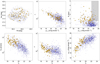 |
Fig. 16 Structural, photometric, and positional properties of galaxies in our sample, with visually selected GC-rich targets identified. The full sample of dwarf galaxies is shown as violet dots. Grey filled circles represent galaxies brighter than IE = 16; the symbol size indicates the galaxy effective radius (upper left panel). Visually identified GC-rich candidates are denoted by filled orange or empty orange circles (the latter for dwarfs near bright galaxies). The grey shaded area in the upper right panel represents the expected locus for UDGs, as defined by van Dokkum et al. (2015) and in Sect. 6. |
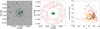 |
Fig. 17 GC selection procedure. Left panel: IE image of the dwarf EDwC-0791. The green circle shows the 1.5 Re search radius adopted to identify GC candidates around the galaxy. Middle panel: on-galaxy selection region (large central green circle) and the first inner background annulus used for background correction (red circles, 5–10 Re in size). All sources detected on the galaxy and in the background region are shown as green (on-galaxy) and red (off-galaxy) empty circles. The sources that fulfil all selection criteria adopted for identifying GC candidates are shown as filled red (green) symbols in the outer (inner) area. The blue symbols in the centre identify GC candidates within Re/3, which are possible nuclear star clusters. Right panel: concentration index for sources on the galaxy and in the first background annulus. The symbols and colours are the same as in the middle panel. The dashed orange lines and the pale orange shaded area mark the ranges adopted for identifying GC candidates in this plane. The magenta line is the median concentration index measured on bright stars. |
6.5.2 GC richness from automatic detection
Using the photometric catalogue of Kluge et al. (2025) we conducted a comprehensive analysis of detected sources to identify and characterise GC candidates associated with each galaxy in our footprint of the Perseus cluster (Table A.2). To estimate the total GC population, we made several assumptions and adopted the procedures already used in the literature (e.g. Cantiello et al. 2020) and outlined below.
At the distance of Perseus, the typical size of a GC, assuming a half-light radius of 3 pc based on Milky Way GCs (Harris 1996), is about one order of magnitude smaller than the typical FWHM of the data in question. Therefore, these sources can be considered point-like in the ERO Perseus dataset.
Initially, we extracted galaxy characteristics (position, effective radius Re, etc.; Table A.2) to identify all sources in the photometric catalogue within 1.5 Re of each galaxy (Lim et al. 2018). We adopted 3.7 Re for bright galaxies (Forbes et al. 2017). Additionally, sources within 3 background annuli with inner and outer radii equal to 5 and 10 Re, 10 and 13.25 Re, and 13.25 and 15.9 Re , were identified around each galaxy. We then estimated three overdensity values of sources on-galaxy (one value for each background annulus) by subtracting the off-galaxy density from the on-galaxy density. The number of extra sources on-galaxy was then obtained by multiplying the overdensity by the effective area of the galaxy. We chose not to apply a further factor of 2 due to spatial coverage, based on a series of empirical tests derived from estimates of NGC within 4 Re . By comparing the total GC population estimated within 1.5 and 4.0 Re, we find that not doubling the population within 1.5 Re provides a better match with the results within 4 Re (which are spatially more complete). We adopted as reference the central value of the three estimates derived using all background annuli. The numbers and their uncertainties are reported in Table A.2. Using the same sample of selected GC candidates on-galaxy, we also counted the number of objects within Re /3 of the galaxy photocentre, where one or more sources may potentially be nuclear star clusters. The number of these candidates,  , is also reported in Table A.2.
Subsequently, we refined the analysis to consider only sources that satisfied certain properties for compactness, such as concentration index, FWHM, and elongation. To further narrow down the GC candidate list, we restricted the analysis to compact sources within the expected turnover magnitude (TOM),  , at the distance of Perseus. For
  we assumed the distance modulus m–M = 34.3, and derived an absolute TOM of M(IE)TOM ≋ –8.0 (see also Saifollahi et al. 2025). This corresponds to assuming
  (Rejkuba 2012, and references therein) adjusted by a 0.5 offset from the V band to the IE band. Consequently, the expected TOM in IE is approximately 26.3. For the bright cut-off for GC candidates, we considered using a magnitude of 22.7, estimated assuming a 3σGCLF cut brighter than the expected TOM, adopting a GC luminosity function (GCLF) width of σGCLF = 1.2. Although σGCLF = 1.0 or smaller is more in line with expectations for dwarfs (Villegas et al. 2010), we opted for a larger value due to the (fractionally small) depth of the cluster and the wide range of galaxy magnitudes we consider.
Finally, adopting the procedure described above for assessing the excess of sources on galaxies, and assuming that the GC candidates sample is basically complete at the peak of the GCLF (Kluge et al. 2025), we double the number of selected sources for an estimate of the total population of GC on the galaxy, NGC , under the assumption of Gaussian GCLF. The entire procedure adopted is depicted in Fig. 17, for the dwarf galaxy EDwC-0791.
As a preliminary test, we compared the GC richness results obtained through visual inspection with the number of GC candidates, NGC , extracted using the procedure described above. Figure 18 shows NGC versus IE, colour-coded based on the GC richness score obtained from our initial visual inspection (as labelled). The upper panel shows the full sample in logarithmic scale, while the bottom panel displays only the sample of dwarf galaxies over a limited range of NGC , adopting a linear scale.
An initial notable finding is that, except for one dwarf (EDwC-0055), all 37 galaxies with a visual GC richness score of 1 (7/7) are estimated to have a population of NGC > 0. The case of EDwC-0055 – shown in the upper left panel of Fig. 14 – is intriguing: despite not being in proximity to any apparent source of GC contamination, it exhibits a clear concentration of point-like sources within Re/2 and visually appears GC-rich according to our adopted definition. We made several tests on the estimated NGC value for this galaxy and found it to be robust against changes in the background regions used. A key factor influencing the outcome might be the presence of three pointlike sources close in projection in the galaxy core, which might impact the algorithms for compactness selection. Furthermore, adopting a fainter magnitude limit for GC selection, the NGC for this galaxy indeed makes it GC-rich. This may suggest that the galaxy lies in the background of the cluster or that its GC population is skewed towards fainter magnitudes due to sample size effects, or a combination of both.
Expanding the comparison to objects with a visual GC score of ≥ 0.85 (equivalent to six out of seven total votes in favour of GC richness), out of 70 dwarfs, four exhibit NGC = 1, while the rest have NGC > 2, thus effectively meeting our visual definition of GC richness. A final note regarding the comparison between visual and automated richness assessments is that, in all cases with a score of ≥ 0.85, the two estimates are consistent within the NGC uncertainties reported in Table A.2, which were estimated from the Poisson scatter of the three background regions.
In Fig. 19, we present the same structural, photometric and positional properties of the galaxy sample as shown in Fig. 16, in this case using the estimated NGC values rather than visual classification. To identify GC-rich dwarfs quantitatively, we first determined the median population of GCs for dwarf galaxies with NGC > 1, and found 〈NGC〉 = 4. Then, we further constrained the GC-richness by measuring its robustness against our estimated uncertainty. Specifically, we required ∆NGC/NGC ≤ 0.5, i.e. imposing that the fractional error on NGC must be less than or equal to 50%. In the figure we adopt for bright, dwarf and GC-rich (contaminated and uncontaminated) galaxies the same symbol and colour coding as Fig. 16. Furthermore, the symbol sizes of bright (grey dots in the upper left panel) and GC-rich dwarfs (orange circles in all panels) scale with the total population of GC candidates, adopting different scaling factors for bright and dwarf galaxies for clarity. The overall consistency of the results shown in Figs. 16 and 19 provides evidence of the validity of the visual inspection approach adopted, with the additional evidence that brighter galaxies tend to host a larger GC population.
In the upper panel of Fig. 18, we also present the NGC estimates for the bright galaxies in the field. The approach adopted here, as described above, is probably not optimal for bright galaxies or close to regions with strong GC count gradients. This is because the background correction to NGC in the more contaminated inner cluster regions, when using our criteria, might not be optimal and would need to be fine-tuned for each single bright galaxy. For the purposes of this work, however, we maintain the current procedure.
Despite this limitation, the upper panel of Fig. 18 shows the expected correlation between NGC and IE, i.e. between the total GC population (total GC mass) and the galaxy mass (Spitler & Forbes 2009; Burkert & Forbes 2020), spanning approximately ten magnitudes and about three orders of magnitude in NGC , including the bright and massive galaxies in our sample. In this panel, we plot the linear fit equation to log10 NGC versus IE, adopting different IE magnitude intervals (see figure caption) and including all galaxies with NGC > 4. Although the scatter is notably large – especially considering that both quantities are in log scale – the known correlation is well identified. A linear fit to these data for the range of 10 ≤ IE ≤ 21 appears to align with the entire dataset of magnitudes and log10 NGC values (Pearson correlation coefficient r = –0.8). However, we find that the slope of the NGC–magnitude relation changes for galaxies fainter than IE = 17. Therefore, our results seem to support similar analyses from the literature about the flattening of the NGC–magnitude relation for faint galaxies (Harris et al. 2013; Burkert & Forbes 2020; Jones et al. 2023). Further refinements are in progress, with a more specific selection of GCs around bright galaxies and possibly involving a colour selection in the GC identification procedure using the NISP data.
The left panel of Fig. 20 shows the positions of the dwarfs in the field (violet circles), with symbol size scaled to the GCs specific frequency  . In the panel, we also show the positions of galaxies in the five brightest magnitude ranges (8 ≤ IE ≤ 13), indicated by grey circles. While we find that galaxies with the largest NGC are scattered around the field, inspecting SN it appears that galaxies located around the east–west strip, where most of the brightest cluster members are found, tend to exhibit larger S N values on average, especially south of the BCG region.
In the middle panel of Fig. 20, we plot the NGC values versus the clustercentric radius, RCl , measured with respect to the BCG. In general, there seems to be no compelling evidence of a correlation between NGC or SN and RCl.
As a final test for the GC populations in dwarf and bright galaxies in the field, we compared the S N versus V band magnitude relation for our entire sample with the mean relations derived for UDGs in the Coma cluster (Lim et al. 2018) and in Virgo (Lim et al. 2020), all shown in the right panel of Fig. 20. Ignoring the elements with NGC < 4, where the population is typically consistent with zero within uncertainties, our S N estimates for dwarfs appear to range between the Virgo and Coma mean relations. Previous studies have shown that low- mass galaxies in denser environments can have higher SN (Peng et al. 2008; Mistani et al. 2016; Lim et al. 2018). Therefore, our results possibly indicate that Perseus is dynamically intermediate: not as evolved and relaxed as Coma is, not as active as and still in evolution as Virgo is. For the bright galaxy component, i.e., all galaxies with IE < 16.3, we estimate a median 〈S N〉 = 0.9, which appears slightly smaller than the average for galaxies of this magnitude (Harris et al. 2017). However, the scatter is quite large, and, as explained above, the procedure adopted here to estimate NGC for bright targets will probably require further refinements, which will be subject of a future dedicated paper.
As a final note, we encourage approaching the GC selection presented in this section with due consideration. It is based on morphometric and photometric selection from single-band data, along with statistical background decontamination. However, potential residual contamination on the galaxy or in the background estimation regions, coupled with spatially changing background (particularly relevant for brighter galaxies and around bright companions), represents a significant limitation that may affect our estimates of NGC . To enhance our analysis, future observations with spatial resolution and depth similar to VIS, especially in the near-IR (e.g. from Roman or JWST), are required. These observations will provide the necessary colour constraints for a more robust cleaning of the sample from interlopers.
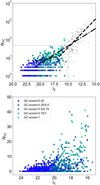 |
Fig. 18 Total GC population vs galaxy IE magnitude for the full sample of galaxies (upper panel, log scale on the y-axis) and for the sample limited to faint IE < 15 galaxies (lower panel, linear y-scale). The full sample is represented by grey filled circles in the upper panel. Dwarf galaxies are symbol and colour-coded based on their GC richness score, as labelled. In the upper panel, we also report fits to the data using the sample of galaxies with 10 ≤ IE ≤ 21 and NGC ≥ 5 (dash-dotted line), as well as a broken linear fit (dashed line) obtained adopting a separation limit at IE = 17. The dotted box in the upper panel shows the position of the box in the lower panel. |
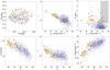 |
Fig. 19 Same as in Fig, 16, except that GC-richness is determined through automatic GC detection. The symbol sizes scale for bright galaxies (grey symbols in the upper right panel) and for the dwarf population (orange symbols in all panels) according to the total population of identified GC candidates, NGC , adopting different scaling factors for bright and dwarf galaxies for clarity. |
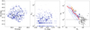 |
Fig. 20 Galaxy positions and GC content. Left panel: violet circles indicate the positions of dwarf galaxies, with symbol size scaled to the specific frequency, S N. Grey circles mark the brightest galaxies in the field, with magnitudes 8 ≤ IE ≤ 13. Middle panel: total population of GC candidates in dwarf galaxies, NGC (log scale), plotted against the clustercentric distance, RCl , from the BCG. The symbol sizes correspond to those in the left panel. Right panel: specific frequency vs. magnitude plot. The colours and symbols are as in the left panel, except that the symbol size is scaled to NGC. The red curve shows the relation from Lim et al. (2020) for UDGs in Virgo, while the orange curve is for UDGs in Coma (Lim et al. 2018). The horizontal dashed line shows the S N = 1 level. |
6.6 Two-dimensional spatial distribution
In Fig. 21 we show the projected distribution and the density map and contours of the Perseus dwarf galaxies and UDGs across the ERO FoV. The projected density of the bright galaxy sample from Cuillandre et al. (2025b) is also shown in the same figure.
The dwarf distribution has two main iso-density centres located on each side of the bright galaxy distribution. The main iso-density centre is located approximately at RA = 3h19m12s.0 and Dec = 41°30′0.″0 and the second one, located to the left of the main iso-density centre, is centred approximately at RA = 3h20m8.S4, Dec = 41°32′42.″0. The double iso-density centre could be the result of recent merger activity reported for this cluster. It is worth noting that the bright galaxies were not removed from the image when the data were visually inspected for the identification of dwarfs in the field via the annotation tool. Therefore, we may be missing a handful of dwarfs that are within the halo of the massive (bright) galaxies.
Figure 21 also shows the iso-density centre of the GCs and the isophotal centre of the ICL at semimajor-axis radius 320 kpc measured by Kluge et al. (2025). The ICL isophotal centre is measured at (3h19m22.S253,41°31′58.″902) and the GC isodensity centre at (3h19m35.S031,41°31′22.″ 108). The ICL isopho- tal centre is located westward of the BCG core by 60 kpc (Kluge et al. 2025). The comparison of the location of the dwarfs, GCs, and ICL in the ERO field indicates that all three distributions appear to have a main centre displaced to the west of the galaxy light distribution, with the dwarf main centre being the most displaced (about 110 kpc) from the BCG. This agreement likely indicates that these shifts are real and not driven by some bias introduced in the data reduction and analysis. The brightest X- ray emission is centred on the BCG and only on larger scales is offset to the east, i.e., opposite to the ICL (Kluge et al. 2025).
The 2D projected distribution of UDGs appears strongly asymmetric with respect to the cluster centre, showing a large offset to the west of the iso-density centres of the dwarf distribution. An asymmetry of the UDGs with respect to the cluster centre has also been reported for the Virgo and Hydra I cluster (Lim et al. 2020; La Marca et al. 2022). For the Hydra I cluster, roughly half of the UDGs are concentrated close to the cluster core, in the same direction as the GCs and ICL centres, and around a subgroup of galaxies to the north, while the other half are found uniformly distributed at larger clustercentric distances. We also note a similar split in the distribution for the UDGs in Perseus, with approximately half concentrated in the west overdensity and the remaining half found more uniformly distributed at larger clustercentric distances. There is a hint that the spatial distribution of the UDGs may be associated with overdensities of bright galaxies in the cluster. This would be consistent with the findings for other galaxy clusters where overdensities of UDGs are found close to subgroups of galaxies (Janssens et al. 2019). If the UDGs are associated with the grouping of bright galaxies, this may suggest that the UDGs joined the cluster via accretion of subgroups. On the other hand, we cannot rule out that they could also be native to the cluster (Sales et al. 2020).
7 Conclusions
As part of the Euclid ERO series of papers, we have used Euclid imaging of the Perseus cluster to demonstrate the capabilities of the telescope for dwarf galaxy science. The depth, spatial resolution, and FoV have allowed us to detect and characterise 1100 dwarf galaxy candidates in a 0.7 deg2 field, slightly offset from the BCG, NGC 1275. We visually classified their morphologies, extracted their photometric and structural properties, quantified their GC populations, and mapped their spatial distribution across the cluster. Some of our key findings are highlighted below:
- –
With 1100 dwarf candidates, this catalogue more than doubles the number of dwarfs associated with the Perseus cluster in the literature. The detections appear to be robust, and the dwarfs follow known scaling relations in the literature, although the diffuse end of the dwarf parameter relations are more densely populated than in previous studies. Morphologically, the sample can be separated into: 96% [4%] dEs [dIs]; 53% [47%] nucleated [nonnucleated]; 74% [26%] GC-poor [GC-rich], and 94% [6%] not morphologically disturbed [morphologically disturbed]. Furthermore, 8% of the dwarfs can be classified as UDGs. The UCDs were not considered during the visual examination of the images due to their small sizes and relatively high surface brightnesses.
- –
The nucleated dwarfs in the Perseus cluster follow the same trends found in the literature, with nuclei typically found in brighter, larger, and rounder dwarfs with flatter surface brightness profiles. In this work, however, we also illustrated the potential for Euclid to identify complex nuclear structures; it appears that several nuclei are associated with tidal features, suggesting that we are witnessing formation or transformation events. With the large number of dwarfs expected from the EWS, we may be able to place observational constraints on the frequency of these events.
- –
The combination of the surface brightness sensitivity, spatial resolution, and wide field of Euclid allowed us to detect and characterise the GC systems of the dwarf galaxies. We automated the GC detection, and the resulting correlation between NGC and IE , including the flattening below IE ~ 17, agrees well with the literature. In terms of distribution, the dwarfs with the highest GC counts can be found scattered throughout the cluster, but those with the highest SN values are typically concentrated south of the BCG, potentially another indication of a recent merger. Our SN estimates for the Perseus dwarfs appear to range between the mean relations of those in the Virgo and Coma clusters, suggesting that Perseus is dynamically intermediate, neither as active as the Virgo cluster nor as relaxed as the Coma cluster.
- –
We compared the 2D projected distribution of the dwarfs in the cluster with those of both the GCs and ICL distributions (Kluge et al. 2025). The dwarf distribution is characterised by a double iso-density centre, perhaps due to a recent merger event. The main iso-density centre of this distribution is shifted to the west of the BCG, in agreement with the iso-density centre of the GCs and the isophotal centre of the ICL at semimajor-axis radius 320 kpc. The UDGs show a more asymmetric distribution than the dwarf population as a whole; roughly half of the UDGs are located westward of the cluster centre, in the same direction as the GC iso-density centre and the ICL isophotal centre, while the other half can be found more uniformly distributed at larger clustercentric distances. There is a hint that the spatial distribution of the UDGs may be associated with overdensities of bright galaxies in the cluster, which could indicate their recent accretion via groups. However, we cannot rule out that they may also be native to the cluster.
The ERO VIS and NISP images of the Perseus cluster have demonstrated the capability of Euclid to not only detect new LSB galaxies, including those close to bright stars, but more importantly, to identify them as genuine dwarf galaxies. The pristine PSF and high spatial resolution of Euclid provide the ability to distinguish dwarfs from other sources, such as background galaxies, without the need to perform follow-up observations. Furthermore, we showed that Euclid offers the added benefit of being able to also provide a census of the GC systems and nuclei associated with the dwarfs. In particular, looking for high concentrations of GCs in the Euclid surveys shows great potential for the detection of GC-rich dwarfs and UDGs.
The upcoming EWS will have a sky coverage ~14 000 deg2. Although it is expected to be about 0.75 mag arcsec−2 less deep in NISP than the data presented in this work and to have a LSB performance in VIS similar to the ERO Perseus image (due to the effect of Galactic cirrus in the ERO Perseus field), it will transform our ability to characterise dwarf galaxies across a range of stellar masses and located in a variety of environments. The analysis of such a large dataset will require the development of automatic detection methods, which are currently underway. The dwarf catalogue presented here should prove to be a useful benchmark for testing present and future machine learning techniques.
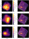 |
Fig. 21 Two-dimensional distribution of the dwarf and ultra diffuse galaxies in the ERO Perseus cluster field. Top left: projected distribution (white dots) and density map of the 1100 dwarf candidates within the Euclid ERO FoV of the Perseus cluster. Top right: density map (white contours) of the dwarf candidates are overlaid on the Euclid ERO IE image of the cluster. Middle left and right: same as above, but for the ultra diffuse galaxies identified as cluster members. Bottom left and right: same as above, but for the bright (non-dwarf) galaxies identified as cluster members. The iso-density centres of the dwarfs, as well as the iso-density centre of the GCs and the isophotal centre of the ICL at semimajor-axis radius 320 kpc, are indicated with the two red, green, and blue crosses, respectively. |
Data availability
Full Tables A.1–Tables A.3 and B.1 are available at the CDS via anonymous ftp to cdsarc.cds.unistra.fr (130.79.128.5) or via https://cdsarc.cds.unistra.fr/viz-bin/cat/J/A+A/697/A12.
Acknowledgements.
This work has made use of the Early Release Observations (ERO) data from the Euclid mission of the European Space Agency (ESA), 2024, https://doi.org/10.57780/esa-qmocze3. The Euclid Consortium acknowledges the European Space Agency and a number of agencies and institutes that have supported the development of Euclid, in particular the Agenzia Spaziale Italiana, the Austrian Forschungsförderungsgesellschaft funded through BMK, the Belgian Science Policy, the Canadian Euclid Consortium, the Deutsches Zentrum für Luft- und Raumfahrt, the DTU Space and the Niels Bohr Institute in Denmark, the French Centre National d’Etudes Spa- tiales, the Fundação para a Ciência e a Tecnologia, the Hungarian Academy of Sciences, the Ministerio de Ciencia, Innovación y Universidades, the National Aeronautics and Space Administration, the National Astronomical Observatory of Japan, the Netherlandse Onderzoekschool Voor Astronomie, the Norwegian Space Agency, the Research Council of Finland, the Romanian Space Agency, the State Secretariat for Education, Research, and Innovation (SERI) at the Swiss Space Office (SSO), and the United Kingdom Space Agency. A complete and detailed list is available on the Euclid web site (http://www.euclid-ec.org). This work has made use of the Early Release Observation (ERO) data from the Euclid mission of the European Space Agency (ESA), 2024, https://doi.org/10.57780/esa-qmocze3. O.M. would like to acknowledge Thomas Boch and Matthieu Baumann at the Observatoire de Strasbourg. M.P. and A.V. are both supported by the Academy of Finland grant number 347089. A.F. acknowledges support from RYC2021-031099-I and PID2021-123313NA-I00 of MICIN/ AEI/10.13039/501100011033/FEDER,UE,NextGenerationEU/PRT. L.H., R.S., M.C., and R.H. acknowledge funding from the Italian INAF Large Grant 12-2022.
Appendix A Properties of the dwarf galaxy candidates
The dwarf galaxy candidates are classified by visual inspection with the methodology described in Sect. 3. The final sample contains 1100 dwarf galaxies of which 96% are classified as dE, and 4% as dI. The dE galaxies are further classified as nucleated (53%), GC-rich (26%), and with disturbed morphology (6%).
Table A.1 lists the entire sample of dwarf galaxy candidates, ordered by increasing RA. The column definitions are as follows: a unique identifier (ID), RA in degrees, Dec in degrees, morphology (either dE or dI), GC-rich flag (recall that in the visual classification we defined dwarfs with NGC > 2 GCs as GC-rich), a flag for the presence of a nucleus (Nucleated), and a disturbed morphology flag (Disturbed). Both dE and dI galaxies could be classified as disturbed.
Table A.2 lists the photometric and structural parameters of the dwarf galaxy candidates (ordered by increasing RA) obtained with the methodology described in Sect. 5. The column definitions are as follows: a unique identifier (ID), RA in degrees, Dec in degrees, apparent magnitude in the IE filter (IE), effective radius in arcsec (Re), Sérsic index (n), axis ratio (AR), position angle in radians (PA), central surface brightness (µIE,0, mag arcsec−2), surface brightness at Re (µIE,0, mag arcsec−2), surface brightness within Re (〈µIE,0〉, mag arcsec−2), the number of associated GCs which has been corrected for background and completeness (NGC), and the number of GCs and NSCs within Re/3 of the galaxy photocentre ( ).
).
Table A.3 lists the aperture magnitudes and extinction corrections (EC) described in Sect. 5.4 and 5.1, respectively. The column definitions are: a unique identifier (ID), the apparent magnitude in the IE filter, the extinction correction in IE , the apparent magnitude in the YE filter, the extinction correction in YE , apparent magnitude in the JE filter, the extinction correction in JE , the apparent magnitude in the HE filter, and the extinction in HE . The dwarf galaxy candidates are ordered by increasing RA.
Finally, images of the 1100 dwarf galaxy candidates in the final sample of this work are shown in Fig. A.1. The cutouts were created from the IE image. For better visibility, the dimensions of each cutout have been scaled to twice the area of the original annotations and an arcsinh stretch has been applied. The dwarf candidates are ordered by decreasing surface brightness 〈µIE,e〉.
Visual properties of the dwarf galaxy candidates. (†)
Photometric and structural properties of the dwarf galaxy candidates.(†)
Aperture magnitudes and extinction corrections (EC) in the Euclid YE, JE, and HE bands for each dwarf galaxy candidate.(†)
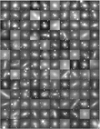 |
Fig. A.1 Cutouts of the IE image with arcsinh stretching of all our dwarf candidates, ordered by decreasing surface brightness 〈µIE,e〉. The size of the cutouts are proportional to twice the area determined from the annotation of the classifiers; north is up and east is to the left. The figure continues on the next pages. |
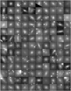 |
Fig. A.1 Continued |
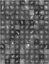 |
Fig. A.1 Continued |
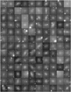 |
Fig. A.1 Continued |
 |
Fig. A.1 Continued |
 |
Fig. A.1 Continued |
 |
Fig. A.1 Continued |
 |
Fig. A.1 Continued |
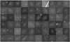 |
Fig. A.1 Continued |
Appendix B Visual properties of the galaxies not included in the final dwarf catalogue
The final catalogue of dwarf galaxies presented in Appendix A is based on the voting system presented in Sect. 3. A score of 0.7 (corresponding to the agreement of 5/7 classifiers) was the threshold we adopted to keep or reject a galaxy from the final catalogue. Some 160 objects from our initial list of 1260 galaxies fall below this threshold and were subsequently removed from the sample. Nevertheless, these are galaxies that were initially flagged as potential dwarf candidates by at least two team members, and may include some legitimate dwarf galaxies; hence, we include their properties here. Table B.1 presents the visual properties of the candidates, ordered by increasing RA. The column definitions are as follows: a unique identifier (ID), RA in degrees, Dec in degrees, morphology (either dE or di), a GC-rich flag (where dwarfs with Ngc > 2 GCs were considered GC-rich), a flag denoting the presence of a nucleus (Nucleated), and a flag for galaxies with disturbed morphologies (Disturbed).
Images of these rejected candidates are shown in Fig. B.1. The cutouts were created from the IE image. For better visibility, the dimensions of each cutout have been scaled to twice the area of the original annotations and an arcsinh stretch has been applied. The dwarf candidates are ordered by increasing RA.
Visual properties of the dwarf galaxy candidates not included in the final catalogue.(†)
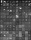 |
Fig. B.1 Cutouts of the IE image with arcsinh stretching of the 160 objects rejected as dwarf candidates, ordered by increasing right ascension. The size of the cutouts are proportional to twice the area determined from the annotation of the classifiers; north is up and east is to the left. The figure continues on the next page. |
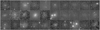 |
Fig. B.1 Continued |
Appendix C A visual comparison of the Euclid dwarf sample with pre-existing catalogues
The differences between the Euclid dwarf sample and previous catalogues in the literature can be more clearly illustrated with figures. In Sect. 4, we discussed how the Euclid dwarf candidates compare with those identified in pre-existing catalogues. Here, we examine the converse, how the properties of dwarf galaxies in the three largest published catalogues compare against the Euclid dwarf sample. For this comparison, we restrict the literature samples to those galaxies with a match in the Euclid dwarf catalogue (see Sect. 4 for a discussion of the completeness of these matches). Furthermore, for consistency, we use parameters measured on the Euclid ERO images for all galaxies.
In Fig. C.1, C.2, and C.3, we compare the effective radius, apparent magnitude, and central surface brightnesses of the dwarf candidates in the Euclid catalogue with those in the Kang et al. (2024), Meusinger et al. (2020), and Wittmann et al. (2019) catalogues, respectively. As the Kang et al. (2024) and Meusinger et al. (2020) catalogues extend beyond the Euclid FoV, we compare the matched galaxies with the full Euclid dwarf sample. For the Wittmann et al. (2019) catalogue, which has a smaller footprint, we only compare their sample against the subset of Euclid dwarfs that fall within the FoV of the WHT imaging. It should also be noted that we match against the full literature catalogues here; we do not distinguish between cluster members, non-members, or unconfirm From Fig. C.1 and C.2, it becomes clear that the Kang et al. (2024) and Meusinger et al. (2020) samples focused more on the brighter galaxies, and explains why our sample has so many more dwarf candidates.
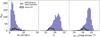 |
Fig. C.1 Comparison of basic properties (effective radius, apparent magnitude, and central surface brightness) of the full Euclid dwarf sample against the matched galaxies in Kang et al. (2024). For consistency, all of the plotted values are those measured on the Euclid images. |
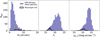 |
Fig. C.2 Comparison of basic properties (effective radius, apparent magnitude, and central surface brightness) of the full Euclid dwarf sample against the matched galaxies in Meusinger et al. (2020). For consistency, all of the plotted values are those measured on the Euclid images. |
On the other hand, the Wittmann et al. (2019) sample covers a similar parameter space, but it would appear that the Euclid imaging is slightly deeper. Given the shape of the luminosity function (Cuillandre et al. 2025b), this difference is enough to yield a relatively large number of new, faint dwarfs in this region, as seen in Fig. C.3.
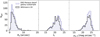 |
Fig. C.3 Comparison of basic properties (effective radius, apparent magnitude, and central surface brightness) of the full Euclid dwarf sample against the matched galaxies in Wittmann et al. (2019). For consistency, all of the plotted values are those measured on the Euclid images. For comparison, we only plot the subsample of Euclid dwarf candidates that fall within the FoV of the Wittmann et al. (2019) data. |
Appendix D Euclid NISP-NISP colours as a function of VIS magnitude IE
Following the discussion of the colours in Sect. 5.1, we also include the Euclid NISP-NISP colours in Fig. D.1.
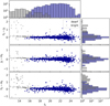 |
Fig. D.1 Euclid NISP-NISP colours as a function of IE measured using aperture photometry within 1 Re of the 1100 dwarf galaxy candidates and the bright galaxy sample in the ERO Perseus field from Cuillandre et al. (2025b) shown in violet and light-grey colours, respectively. The magnitudes were corrected for extinction before the colours were computed, as described in Sect. 5.1. |
References
- Aguerri, J. A. L., Girardi, M., Agulli, I., et al. 2020, MNRAS, 494, 1681 [NASA ADS] [CrossRef] [Google Scholar]
- Andreon, S. 1994, A&A, 284, 801 [NASA ADS] [Google Scholar]
- Astropy Collaboration (Robitaille, T. P., et al.) 2013, A&A, 558, A33 [NASA ADS] [CrossRef] [EDP Sciences] [Google Scholar]
- Astropy Collaboration (Price-Whelan, A. M., et al.) 2018, AJ, 156, 123 [Google Scholar]
- Astropy Collaboration (Price-Whelan, A. M., et al.) 2022, ApJ, 935, 167 [NASA ADS] [CrossRef] [Google Scholar]
- Bender, R., Burstein, D., & Faber, S. M. 1992, ApJ, 399, 462 [NASA ADS] [CrossRef] [Google Scholar]
- Bender, R., Kormendy, J., Cornell, M. E., & Fisher, D. B. 2015, ApJ, 807, 56 [Google Scholar]
- Bertin, E. 2011, ASP Conf. Ser., 442, 435 [Google Scholar]
- Bertin, E., & Arnouts, S. 1996, A&AS, 117, 393 [NASA ADS] [CrossRef] [EDP Sciences] [Google Scholar]
- Binggeli, B. 1994, Euro. Southern Observ. Conf. Workshop Proc., 49, 13 [Google Scholar]
- Binggeli, B., & Cameron, L. M. 1991, A&A, 252, 27 [NASA ADS] [Google Scholar]
- Binggeli, B., & Jerjen, H. 1998, A&A, 333, 17 [NASA ADS] [Google Scholar]
- Binggeli, B., Tammann, G. A., & Sandage, A. 1987, AJ, 94, 251 [Google Scholar]
- Blakeslee, J. P., Jordán, A., Mei, S., et al. 2009, ApJ, 694, 556 [Google Scholar]
- Bonnarel, F., Fernique, P., Bienaymé, O., et al. 2000, A&AS, 143, 33 [NASA ADS] [CrossRef] [EDP Sciences] [Google Scholar]
- Boselli, A., Boissier, S., Cortese, L., & Gavazzi, G. 2008, ApJ, 674, 742 [Google Scholar]
- Boselli, A., Fossati, M., Ferrarese, L., et al. 2018, A&A, 614, A56 [NASA ADS] [CrossRef] [EDP Sciences] [Google Scholar]
- Boselli, A., Fossati, M., & Sun, M. 2022, A&A Rev., 30, 3 [NASA ADS] [CrossRef] [Google Scholar]
- Brunzendorf, J., & Meusinger, H. 1999, A&AS, 139, 141 [NASA ADS] [CrossRef] [EDP Sciences] [Google Scholar]
- Burkert, A., & Forbes, D. A. 2020, AJ, 159, 56 [Google Scholar]
- Cantiello, M., Venhola, A., Grado, A., et al. 2020, A&A, 639, A136 [NASA ADS] [CrossRef] [EDP Sciences] [Google Scholar]
- Carlsten, S. G., Greene, J. E., Beaton, R. L., & Greco, J. P. 2022, ApJ, 927, 44 [NASA ADS] [CrossRef] [Google Scholar]
- Conselice, C. J., Gallagher, I., John S., & Wyse, R. F. G. 2002, AJ, 123, 2246 [NASA ADS] [CrossRef] [Google Scholar]
- Conselice, C. J., Gallagher, J. S., III, & Wyse, R. F. G. 2003, AJ, 125, 66 [CrossRef] [Google Scholar]
- Côté, P., Piatek, S., Ferrarese, L., et al. 2006, ApJS, 165, 57 [Google Scholar]
- Cropper, M., Pottinger, S., Niemi, S., et al. 2016, SPIE Conf. Ser., 9904, 99040Q [NASA ADS] [Google Scholar]
- Cuillandre, J.-C., Bertin, E., Bolzonella, M., et al. 2025a, A&A, 697, A6 (Euclid on Sky SI) [Google Scholar]
- Cuillandre, J.-C., Bolzonella, M., Boselli, A., et al. 2025b, A&A, 697, A11 (Euclid on Sky SI) [Google Scholar]
- den Brok, M., Peletier, R. F., Seth, A., et al. 2014, MNRAS, 445, 2385 [NASA ADS] [CrossRef] [Google Scholar]
- Drinkwater, M. J., Jones, J. B., Gregg, M. D., & Phillipps, S. 2000, PASA, 17, 227 [Google Scholar]
- Dunn, J. M. 2010, MNRAS, 408, 392 [Google Scholar]
- Durrell, P. R., Côté, P., Peng, E. W., et al. 2014, ApJ, 794, 103 [NASA ADS] [CrossRef] [Google Scholar]
- Euclid Collaboration (Scaramella, R., et al.) 2022, A&A, 662, A112 [NASA ADS] [CrossRef] [EDP Sciences] [Google Scholar]
- Euclid Collaboration (Schirmer, M., et al.) 2022, A&A, 662, A92 [NASA ADS] [CrossRef] [EDP Sciences] [Google Scholar]
- Euclid Collaboration (Cropper, M., et al.) 2025, A&A, 697, A2 (Euclid on Sky SI) [Google Scholar]
- Euclid Collaboration (Jahnke, K., et al.) 2025, A&A, 697, A3 (Euclid on Sky SI) [Google Scholar]
- Euclid Collaboration (Mellier, Y., et al.) 2025, A&A, 697, A1 (Euclid on Sky SI) [Google Scholar]
- Euclid Early Release Observations 2024, https://doi.org/10.57780/esa-qmocze3 [Google Scholar]
- Fabian, A. C., Sanders, J. S., Allen, S. W., et al. 2011, MNRAS, 418, 2154 [Google Scholar]
- Fahrion, K., Leaman, R., Lyubenova, M., & van de Ven, G. 2022, A&A, 658, A172 [NASA ADS] [CrossRef] [EDP Sciences] [Google Scholar]
- Ferguson, H. C., & Binggeli, B. 1994, A&A Rev., 6, 67 [NASA ADS] [CrossRef] [Google Scholar]
- Ferrarese, L., Côté, P., Jordán, A., et al. 2006, ApJS, 164, 334 [NASA ADS] [CrossRef] [Google Scholar]
- Ferrarese, L., Côté, P., Cuillandre, J.-C., et al. 2012, ApJS, 200, 4 [Google Scholar]
- Ferrarese, L., Côté, P., MacArthur, L. A., et al. 2020, ApJ, 890, 128 [Google Scholar]
- Fisher, D. B., & Drory, N. 2008, AJ, 136, 773 [NASA ADS] [CrossRef] [Google Scholar]
- Forbes, D. A., Alabi, A., Brodie, J. P., et al. 2017, AJ, 153, 114 [Google Scholar]
- Forbes, D. A., Alabi, A., Romanowsky, A. J., Brodie, J. P., & Arimoto, N. 2020, MNRAS, 492, 4874 [Google Scholar]
- Galametz, A., Saglia, R., Paltani, S., Apostolakos, N., & Dubath, P. 2017, A&A, 598, A20 [NASA ADS] [CrossRef] [EDP Sciences] [Google Scholar]
- Gannon, J. S., Forbes, D. A., Romanowsky, A. J., et al. 2022, MNRAS, 510, 946 [Google Scholar]
- Gavazzi, G., Donati, A., Cucciati, O., et al. 2005, A&A, 430, 411 [NASA ADS] [CrossRef] [EDP Sciences] [Google Scholar]
- Geha, M., Blanton, M. R., Yan, R., & Tinker, J. L. 2012, ApJ, 757, 85 [Google Scholar]
- Gordon, K. D., Clayton, G. C., Decleir, M., et al. 2023, ApJ, 950, 86 [CrossRef] [Google Scholar]
- Górski, K. M., Hivon, E., Banday, A. J., et al. 2005, ApJ, 622, 759 [Google Scholar]
- Grebel, E. K., Gallagher, I., John S., & Harbeck, D. 2003, AJ, 125, 1926 [NASA ADS] [CrossRef] [Google Scholar]
- Gunn, J. E., & Gott, J., Richard, I. 1972, ApJ, 176, 1 [NASA ADS] [CrossRef] [Google Scholar]
- Habas, R., Marleau, F. R., Duc, P.-A., et al. 2020, MNRAS, 491, 1901 [NASA ADS] [Google Scholar]
- Harris, W. E. 1996, AJ, 112, 1487 [Google Scholar]
- Harris, W. E., Harris, G. L. H., & Alessi, M. 2013, ApJ, 772, 82 [Google Scholar]
- Harris, W. E., Blakeslee, J. P., & Harris, G. L. H. 2017, ApJ, 836, 67 [Google Scholar]
- Hilker, M., Infante, L., Vieira, G., Kissler-Patig, M., & Richtler, T. 1999, A&AS, 134, 75 [NASA ADS] [CrossRef] [EDP Sciences] [Google Scholar]
- Hoyer, N., Neumayer, N., Georgiev, I. Y., Seth, A. C., & Greene, J. E. 2021, MNRAS, 507, 3246 [NASA ADS] [CrossRef] [Google Scholar]
- Hoyer, N., Neumayer, N., Seth, A. C., Georgiev, I. Y., & Greene, J. E. 2023, MNRAS, 520, 4664 [CrossRef] [Google Scholar]
- Hunt, L., Annibali, F., Cuillandre, J.-C., et al. 2025, A&A, 697, A9 (Euclid on Sky SI) [NASA ADS] [CrossRef] [EDP Sciences] [Google Scholar]
- Iodice, E., Capaccioli, M., Grado, A., et al. 2016, ApJ, 820, 42 [Google Scholar]
- Janssens, S. R., Abraham, R., Brodie, J., Forbes, D. A., & Romanowsky, A. J. 2019, ApJ, 887, 92 [Google Scholar]
- Jones, M. G., Karunakaran, A., Bennet, P., et al. 2023, ApJ, 942, L5 [CrossRef] [Google Scholar]
- Kang, W., Hwang, H. S., Song, H., et al. 2024, ApJS, 272, 22 [Google Scholar]
- Kent, S. M., & Sargent, W. L. W. 1983, AJ, 88, 697 [NASA ADS] [CrossRef] [Google Scholar]
- Kluge, M., Neureiter, B., Riffeser, A., et al. 2020, ApJS, 247, 43 [Google Scholar]
- Kluge, M., Hatch, N., Montes, M., et al. 2025, A&A, 697, A13 (Euclid on Sky SI) [NASA ADS] [CrossRef] [EDP Sciences] [Google Scholar]
- Kormendy, J. 1985, ApJ, 295, 73 [NASA ADS] [CrossRef] [Google Scholar]
- Kormendy, J., & Bender, R. 2012, ApJS, 198, 2 [Google Scholar]
- Kormendy, J., Fisher, D. B., Cornell, M. E., & Bender, R. 2009, ApJS, 182, 216 [Google Scholar]
- La Marca, A., Iodice, E., Cantiello, M., et al. 2022, A&A, 665, A105 [NASA ADS] [CrossRef] [EDP Sciences] [Google Scholar]
- Larson, R. B., Tinsley, B. M., & Caldwell, C. N. 1980, ApJ, 237, 692 [Google Scholar]
- Lauer, T. R., Faber, S. M., Groth, E. J., et al. 1993, AJ, 106, 1436 [Google Scholar]
- Laureijs, R., Amiaux, J., Arduini, S., et al. 2011, ESA/SRE(2011)12, [arXiv:1110.3193] [Google Scholar]
- Leaman, R., & van de Ven, G. 2022, MNRAS, 516, 4691 [Google Scholar]
- Li, D. D., Eadie, G. M., Abraham, R., et al. 2022, ApJ, 935, 3 [Google Scholar]
- Lim, S., Peng, E. W., Côté, P., et al. 2018, ApJ, 862, 82 [Google Scholar]
- Lim, S., Côté, P., Peng, E. W., et al. 2020, ApJ, 899, 69 [CrossRef] [Google Scholar]
- Lisker, T., Grebel, E. K., & Binggeli, B. 2006, AJ, 132, 497 [Google Scholar]
- Lisker, T., Grebel, E. K., Binggeli, B., & Glatt, K. 2007, ApJ, 660, 1186 [Google Scholar]
- Lisker, T., Janz, J., Hensler, G., et al. 2009, ApJ, 706, L124 [Google Scholar]
- Liu, C., Côté, P., Peng, E. W., et al. 2020, ApJS, 250, 17 [NASA ADS] [CrossRef] [Google Scholar]
- Lotz, J. M., Telford, R., Ferguson, H. C., et al. 2001, ApJ, 552, 572 [Google Scholar]
- Marleau, F. R., Habas, R., Poulain, M., et al. 2021, A&A, 654, A105 [NASA ADS] [CrossRef] [EDP Sciences] [Google Scholar]
- Marleau, F. R., Duc, P.-A., Poulain, M., et al. 2024, A&A, 690, A339 [NASA ADS] [CrossRef] [EDP Sciences] [Google Scholar]
- Mateo, M. L. 1998, ARA&A, 36, 435 [NASA ADS] [CrossRef] [Google Scholar]
- Mathews, W. G., Brighenti, F., Faltenbacher, A., et al. 2006, ApJ, 652, L17 [Google Scholar]
- Mayer, L., Governato, F., Colpi, M., et al. 2001, ApJ, 559, 754 [NASA ADS] [CrossRef] [Google Scholar]
- McConnachie, A. W., & Irwin, M. J. 2006, MNRAS, 365, 1263 [Google Scholar]
- Meusinger, H., Rudolf, C., Stecklum, B., et al. 2020, A&A, 640, A30 [NASA ADS] [CrossRef] [EDP Sciences] [Google Scholar]
- Mistani, P. A., Sales, L. V., Pillepich, A., et al. 2016, MNRAS, 455, 2323 [NASA ADS] [CrossRef] [Google Scholar]
- Moore, B., Katz, N., Lake, G., Dressler, A., & Oemler, A. 1996, Nature, 379, 613 [Google Scholar]
- Morrissey, P., Matuszewski, M., Martin, D. C., et al. 2018, ApJ, 864, 93 [Google Scholar]
- Moss, C., & Whittle, M. 2000, MNRAS, 317, 667 [NASA ADS] [CrossRef] [Google Scholar]
- Moss, C., & Whittle, M. 2005, MNRAS, 357, 1337 [Google Scholar]
- Muñoz, R. P., Eigenthaler, P., Puzia, T. H., et al. 2015, ApJ, 813, L15 [Google Scholar]
- Neumayer, N., Seth, A., & Böker, T. 2020, A&A Rev., 28, 4 [NASA ADS] [CrossRef] [Google Scholar]
- Nulsen, P. E. J., & Fabian, A. C. 1980, MNRAS, 191, 887 [Google Scholar]
- Ordenes-Briceño, Y., Puzia, T. H., Eigenthaler, P., et al. 2018, ApJ, 860, 4 [CrossRef] [Google Scholar]
- Pak, M., Paudel, S., Lee, Y., & Kim, S. C. 2016, AJ, 151, 141 [Google Scholar]
- Peng, E. W., Jordán, A., Côté, P., et al. 2008, ApJ, 681, 197 [NASA ADS] [CrossRef] [Google Scholar]
- Peng, C. Y., Ho, L. C., Impey, C. D., & Rix, H.-W. 2010, AJ, 139, 2097 [Google Scholar]
- Penny, S. J., Conselice, C. J., de Rijcke, S., et al. 2011, MNRAS, 410, 1076 [NASA ADS] [CrossRef] [Google Scholar]
- Penny, S. J., Forbes, D. A., & Conselice, C.J. 2012, MNRAS, 422, 885 [Google Scholar]
- Penny, S. J., Forbes, D. A., Pimbblet, K. A., & Floyd, D. J. E. 2014a, MNRAS, 443, 3381 [NASA ADS] [CrossRef] [Google Scholar]
- Penny, S. J., Forbes, D. A., Strader, J., et al. 2014b, MNRAS, 439, 3808 [NASA ADS] [CrossRef] [Google Scholar]
- Planck Collaboration XI. 2014, A&A, 571, A11 [NASA ADS] [CrossRef] [EDP Sciences] [Google Scholar]
- Poulain, M., Marleau, F. R., Habas, R., et al. 2021, MNRAS, 506, 5494 [NASA ADS] [CrossRef] [Google Scholar]
- Rejkuba, M. 2012, Ap&SS, 341, 195 [Google Scholar]
- Saifollahi, T., Zaritsky, D., Trujillo, I., et al. 2022, MNRAS, 511, 4633 [NASA ADS] [CrossRef] [Google Scholar]
- Saifollahi, T., Voggel, K., Lançon, A., et al. 2025, A&A, 697, A10 (Euclid on Sky SI) [NASA ADS] [CrossRef] [EDP Sciences] [Google Scholar]
- Sakai, S., Kennicutt, J., Robert C., & Moss, C. 2012, ApJS, 199, 36 [Google Scholar]
- Sales, L. V., Navarro, J. F., Peñafiel, L., et al. 2020, MNRAS, 494, 1848 [Google Scholar]
- Sánchez-Janssen, R., Côté, P., Ferrarese, L., et al. 2019a, ApJ, 878, 18 [CrossRef] [Google Scholar]
- Sánchez-Janssen, R., Puzia, T. H., Ferrarese, L., et al. 2019b, MNRAS, 486, L1 [CrossRef] [Google Scholar]
- Sérsic, J. L. 1963, Boletin de la Asociacion Argentina de Astronomia La Plata Argentina, 6, 41 [Google Scholar]
- Simon, J. D. 2019, ARA&A, 57, 375 [NASA ADS] [CrossRef] [Google Scholar]
- Smith, R., Davies, J. I., & Nelson, A. H. 2010, MNRAS, 405, 1723 [NASA ADS] [Google Scholar]
- Sola, E., Duc, P.-A., Richards, F., et al. 2022, A&A, 662, A124 [NASA ADS] [CrossRef] [EDP Sciences] [Google Scholar]
- Spitler, L. R., & Forbes, D. A. 2009, MNRAS, 392, L1 [Google Scholar]
- Stone, C. J., Arora, N., Courteau, S., & Cuillandre, J.-C. 2021, MNRAS, 508, 1870 [NASA ADS] [CrossRef] [Google Scholar]
- Stone, C. J., Courteau, S., Cuillandre, J.-C., et al. 2023, MNRAS, 525, 6377 [Google Scholar]
- Su, A. H., Salo, H., Janz, J., Venhola, A., & Peletier, R. F. 2022, A&A, 664, A167 [NASA ADS] [CrossRef] [EDP Sciences] [Google Scholar]
- Tammann, G. A. 1994, Euro. Southern Observ. Conf. Workshop Proc., 49, 3 [Google Scholar]
- Teeninga, P., Moschini, U., Trager, S. C., & Wilkinson, M. H. 2015, in International Symposium on Mathematical Morphology and Its Applications to Signal and Image Processing (Berlin: Springer), 157 [Google Scholar]
- Toloba, E., Boselli, A., Cenarro, A. J., et al. 2011, A&A, 526, A114 [NASA ADS] [CrossRef] [EDP Sciences] [Google Scholar]
- Toloba, E., Guhathakurta, P., Boselli, A., et al. 2015, ApJ, 799, 172 [NASA ADS] [CrossRef] [Google Scholar]
- Torrealba, G., Koposov, S. E., Belokurov, V., & Irwin, M. 2016, MNRAS, 459, 2370 [NASA ADS] [CrossRef] [Google Scholar]
- Trujillo, I., Aguerri, J. A. L., Cepa, J., & Gutiérrez, C. M. 2001, MNRAS, 321, 269 [NASA ADS] [CrossRef] [Google Scholar]
- Tully, R. B., Rizzi, L., Shaya, E. J., et al. 2009, AJ, 138, 323 [NASA ADS] [CrossRef] [Google Scholar]
- Turner, M. L., Côté, P., Ferrarese, L., et al. 2012, ApJS, 203, 5 [NASA ADS] [CrossRef] [Google Scholar]
- Ulmer, M. P., Wirth, G. D., & Kowalski, M. P. 1992, ApJ, 397, 430 [Google Scholar]
- van Dokkum, P. G., Abraham, R., Merritt, A., et al. 2015, ApJ, 798, L45 [NASA ADS] [CrossRef] [Google Scholar]
- Venhola, A., Peletier, R., Laurikainen, E., et al. 2018, A&A, 620, A165 [NASA ADS] [CrossRef] [EDP Sciences] [Google Scholar]
- Venhola, A., Peletier, R., Laurikainen, E., et al. 2019, A&A, 625, A143 [EDP Sciences] [Google Scholar]
- Villegas, D., Jordán, A., Peng, E. W., et al. 2010, ApJ, 717, 603 [Google Scholar]
- Wittmann, C., Lisker, T., Ambachew Tilahun, L., et al. 2017, MNRAS, 470, 1512 [Google Scholar]
- Wittmann, C., Kotulla, R., Lisker, T., et al. 2019, ApJS, 245, 10 [Google Scholar]
- Zanatta, E., Sánchez-Janssen, R., Chies-Santos, A. L., de Souza, R. S., & Blakeslee, J. P. 2021, MNRAS, 508, 986 [NASA ADS] [CrossRef] [Google Scholar]
- Zöller, R., Kluge, M., Staiger, B., & Bender, R. 2024, ApJS, 271, 52 [CrossRef] [Google Scholar]
All Tables
Fraction of nucleated dwarfs as a function of the magnitude and morphology of the host dwarf.
Aperture magnitudes and extinction corrections (EC) in the Euclid YE, JE, and HE bands for each dwarf galaxy candidate.(†)
Visual properties of the dwarf galaxy candidates not included in the final catalogue.(†)
All Figures
|
Fig. 1 Footprint of the VIS image of the Perseus galaxy cluster covering 0.°84 × 0.°84 and overplotted on the PanSTARRS DR1 g + r + i colour image with FoV ~ 1.°17 × 1.°17; north is up and east left. The green circles show the location of the dwarf galaxy candidates identified in the ERO data, while the grey patches represent the footprint of HST/ACS observations (F850LP/SDSSz, F814w, F791w, F785LP, F775w, F625w, F622w filters). The green circles that fall just outside of the Euclid footprint were identified in an earlier data product with a slightly larger FoV. |
| In the text | |
|
Fig. 2 Illustrations of annotated dwarf candidates (red ellipses) and some nuclei (red circles). |
| In the text | |
|
Fig. 3 Agreement between the initial catalogues of the seven classifiers. The catalogues were cross-matched within a 2″ radius, and we counted how many people annotated each object as a dwarf galaxy. |
| In the text | |
|
Fig. 4 VIS-NISP colour image of the Perseus galaxy cluster. The full FoV of 0.°84 × 0.°84 is shown; north is up and east is to the left. Examples of dwarf galaxy candidates are shown in the individual cutouts of size 40″ × 40″. The galaxies EDwC-0854, EDwC-0468, EDwC-0165, and EDwC- 0997 are newly identified UDG candidates. The system composed of EDwC-0141 and EDwC-0145 (bottom right cutout) shows one example of two newly identified dwarfs that appear to be interacting. |
| In the text | |
|
Fig. 5 Classification of the final catalogue of 1100 dwarf galaxy candidates. The darker shades on the outer circle correspond to the presence of the feature of interest. Left: nucleated fraction (outer circle) as a function of morphology (inner circle). Middle left: GC richness (outer circle) as a function of morphology (inner circle). Middle right: signs of disturbed morphology (outer circle) as a function of morphology (inner circle). Right: GC richness (outer circle) as a function of the nucleated fraction. A total of 1061 (96%) dwarf galaxy candidates are classified as dE (dI: 39 or 4%), 581 (53%) are nucleated, 282 (26%) are GC-rich, and 64 (6%) have a disturbed morphology. |
| In the text | |
|
Fig. 6 Cutouts of some dwarf candidates, taken from the VIS-NISP colour image created using the IE band in blue, the YE band in green, and the HE band in red. The colours are projected onto the high-resolution IE band to best reflect their appearance as detected. From top to bottom: dE; nucleated dE; GC-rich dE; disturbed morphologies; multiple nuclei; dI; and GC-rich dI. The sizes of the cutouts are proportional to twice the area determined from the annotation of classifiers; north is up and east is to the left. |
| In the text | |
|
Fig. 7 Map of the colour excess E(B − V) for the dwarf galaxy sample (top) and the bright galaxy sample (bottom) presented in Cuillandre et al. (2025b). |
| In the text | |
|
Fig. 8 PSF models with the native pixel scale of IE , YE , JE, and HE in the centre of the ERO Perseus images. The displayed PSF models have a sidelength of 3″.1 for IE and 9″.3 for YE, JE, and HE. The models are displayed in logarithmic scale. |
| In the text | |
|
Fig. 9 Photometric and structural parameters derived from the surface profile fitting of the 1100 dwarf galaxy candidates and the bright galaxy sample from Cuillandre et al. (2025b) in the ERO Perseus field shown in violet and light grey, respectively. All magnitudes and surface brightness values were corrected for extinction, as described in Sect. 5.1. |
| In the text | |
|
Fig. 10 Euclid VIS-NISP colours as a function of IE measured using aperture photometry within 1 Re of the 1100 dwarf galaxy candidates and the bright galaxy sample in the ERO Perseus field from Cuillandre et al. (2025b) shown in violet and light grey, respectively. The magnitudes were corrected for extinction before the colours were computed, as described in Sect. 5.1. |
| In the text | |
|
Fig. 11 Cutouts of the VIS image for the 93 UDGs in the ERO Perseus field, comprising 8% of the dwarf sample. The UDGs were selected to have an effective radius Re ≥ 1.5 kpc and a central surface brightness in the g band µg,0 ≥ 24 mag arcsec−2. The sizes of the cutouts are proportional to twice the area determined from the annotation of classifiers; north is up and east is to the left. The UDGs are ordered by decreasing surface brightness |
| In the text | |
|
Fig. 12 Comparison between MV, Re, and μV,e scaling relations of the ERO Perseus dwarf sample (violet), including UDGs (orange) from this work, and bright galaxies (black) from Cuillandre et al. (2025b). The basis for this plot is Figure 37 in Kormendy et al. (2009) with updates from Kormendy & Bender (2012), Bender et al. (2015), Kluge et al. (2020), Marleau et al. (2021), and Zöller et al. (2024), including brightest cluster galaxies (BCGs), ellipticals, and classical bulges (dark grey), as well as dwarf galaxies including UDGs (light grey). For the sake of clarity, we do not show the errorbars. The uncertainties vary significantly between the different galaxies. |
| In the text | |
|
Fig. 13 Scaling relations of IE as a function of Re (top), Sérsic index n (middle), and axis ratio (bottom) of the nucleated (pink) and nonnucleated (peach) dEs in the ERO Perseus field. We display the distribution of magnitude for the whole samples, and of the Re, n, and the axis ratio within the same magnitude range 17.3 ≤ IE < 23.6. |
| In the text | |
|
Fig. 14 Examples of dwarfs that stand out due to the number of their nuclei candidates. |
| In the text | |
|
Fig. 15 Examples of dwarfs that stand out due to the presence of a complex nucleus. |
| In the text | |
|
Fig. 16 Structural, photometric, and positional properties of galaxies in our sample, with visually selected GC-rich targets identified. The full sample of dwarf galaxies is shown as violet dots. Grey filled circles represent galaxies brighter than IE = 16; the symbol size indicates the galaxy effective radius (upper left panel). Visually identified GC-rich candidates are denoted by filled orange or empty orange circles (the latter for dwarfs near bright galaxies). The grey shaded area in the upper right panel represents the expected locus for UDGs, as defined by van Dokkum et al. (2015) and in Sect. 6. |
| In the text | |
|
Fig. 17 GC selection procedure. Left panel: IE image of the dwarf EDwC-0791. The green circle shows the 1.5 Re search radius adopted to identify GC candidates around the galaxy. Middle panel: on-galaxy selection region (large central green circle) and the first inner background annulus used for background correction (red circles, 5–10 Re in size). All sources detected on the galaxy and in the background region are shown as green (on-galaxy) and red (off-galaxy) empty circles. The sources that fulfil all selection criteria adopted for identifying GC candidates are shown as filled red (green) symbols in the outer (inner) area. The blue symbols in the centre identify GC candidates within Re/3, which are possible nuclear star clusters. Right panel: concentration index for sources on the galaxy and in the first background annulus. The symbols and colours are the same as in the middle panel. The dashed orange lines and the pale orange shaded area mark the ranges adopted for identifying GC candidates in this plane. The magenta line is the median concentration index measured on bright stars. |
| In the text | |
|
Fig. 18 Total GC population vs galaxy IE magnitude for the full sample of galaxies (upper panel, log scale on the y-axis) and for the sample limited to faint IE < 15 galaxies (lower panel, linear y-scale). The full sample is represented by grey filled circles in the upper panel. Dwarf galaxies are symbol and colour-coded based on their GC richness score, as labelled. In the upper panel, we also report fits to the data using the sample of galaxies with 10 ≤ IE ≤ 21 and NGC ≥ 5 (dash-dotted line), as well as a broken linear fit (dashed line) obtained adopting a separation limit at IE = 17. The dotted box in the upper panel shows the position of the box in the lower panel. |
| In the text | |
|
Fig. 19 Same as in Fig, 16, except that GC-richness is determined through automatic GC detection. The symbol sizes scale for bright galaxies (grey symbols in the upper right panel) and for the dwarf population (orange symbols in all panels) according to the total population of identified GC candidates, NGC , adopting different scaling factors for bright and dwarf galaxies for clarity. |
| In the text | |
|
Fig. 20 Galaxy positions and GC content. Left panel: violet circles indicate the positions of dwarf galaxies, with symbol size scaled to the specific frequency, S N. Grey circles mark the brightest galaxies in the field, with magnitudes 8 ≤ IE ≤ 13. Middle panel: total population of GC candidates in dwarf galaxies, NGC (log scale), plotted against the clustercentric distance, RCl , from the BCG. The symbol sizes correspond to those in the left panel. Right panel: specific frequency vs. magnitude plot. The colours and symbols are as in the left panel, except that the symbol size is scaled to NGC. The red curve shows the relation from Lim et al. (2020) for UDGs in Virgo, while the orange curve is for UDGs in Coma (Lim et al. 2018). The horizontal dashed line shows the S N = 1 level. |
| In the text | |
|
Fig. 21 Two-dimensional distribution of the dwarf and ultra diffuse galaxies in the ERO Perseus cluster field. Top left: projected distribution (white dots) and density map of the 1100 dwarf candidates within the Euclid ERO FoV of the Perseus cluster. Top right: density map (white contours) of the dwarf candidates are overlaid on the Euclid ERO IE image of the cluster. Middle left and right: same as above, but for the ultra diffuse galaxies identified as cluster members. Bottom left and right: same as above, but for the bright (non-dwarf) galaxies identified as cluster members. The iso-density centres of the dwarfs, as well as the iso-density centre of the GCs and the isophotal centre of the ICL at semimajor-axis radius 320 kpc, are indicated with the two red, green, and blue crosses, respectively. |
| In the text | |
|
Fig. A.1 Cutouts of the IE image with arcsinh stretching of all our dwarf candidates, ordered by decreasing surface brightness 〈µIE,e〉. The size of the cutouts are proportional to twice the area determined from the annotation of the classifiers; north is up and east is to the left. The figure continues on the next pages. |
| In the text | |
|
Fig. A.1 Continued |
| In the text | |
|
Fig. A.1 Continued |
| In the text | |
|
Fig. A.1 Continued |
| In the text | |
|
Fig. A.1 Continued |
| In the text | |
|
Fig. A.1 Continued |
| In the text | |
|
Fig. A.1 Continued |
| In the text | |
|
Fig. A.1 Continued |
| In the text | |
|
Fig. A.1 Continued |
| In the text | |
|
Fig. B.1 Cutouts of the IE image with arcsinh stretching of the 160 objects rejected as dwarf candidates, ordered by increasing right ascension. The size of the cutouts are proportional to twice the area determined from the annotation of the classifiers; north is up and east is to the left. The figure continues on the next page. |
| In the text | |
|
Fig. B.1 Continued |
| In the text | |
|
Fig. C.1 Comparison of basic properties (effective radius, apparent magnitude, and central surface brightness) of the full Euclid dwarf sample against the matched galaxies in Kang et al. (2024). For consistency, all of the plotted values are those measured on the Euclid images. |
| In the text | |
|
Fig. C.2 Comparison of basic properties (effective radius, apparent magnitude, and central surface brightness) of the full Euclid dwarf sample against the matched galaxies in Meusinger et al. (2020). For consistency, all of the plotted values are those measured on the Euclid images. |
| In the text | |
|
Fig. C.3 Comparison of basic properties (effective radius, apparent magnitude, and central surface brightness) of the full Euclid dwarf sample against the matched galaxies in Wittmann et al. (2019). For consistency, all of the plotted values are those measured on the Euclid images. For comparison, we only plot the subsample of Euclid dwarf candidates that fall within the FoV of the Wittmann et al. (2019) data. |
| In the text | |
|
Fig. D.1 Euclid NISP-NISP colours as a function of IE measured using aperture photometry within 1 Re of the 1100 dwarf galaxy candidates and the bright galaxy sample in the ERO Perseus field from Cuillandre et al. (2025b) shown in violet and light-grey colours, respectively. The magnitudes were corrected for extinction before the colours were computed, as described in Sect. 5.1. |
| In the text | |
Current usage metrics show cumulative count of Article Views (full-text article views including HTML views, PDF and ePub downloads, according to the available data) and Abstracts Views on Vision4Press platform.
Data correspond to usage on the plateform after 2015. The current usage metrics is available 48-96 hours after online publication and is updated daily on week days.
Initial download of the metrics may take a while.