| Issue |
A&A
Volume 697, May 2025
Euclid on Sky
|
|
|---|---|---|
| Article Number | A10 | |
| Number of page(s) | 28 | |
| Section | Extragalactic astronomy | |
| DOI | https://doi.org/10.1051/0004-6361/202450784 | |
| Published online | 30 April 2025 | |
Euclid: Early Release Observations – Globular clusters in the Fornax galaxy cluster, from dwarf galaxies to the intracluster field★
1
Université de Strasbourg, CNRS, Observatoire astronomique de Strasbourg, UMR 7550,
67000
Strasbourg, France
2
Kapteyn Astronomical Institute, University of Groningen,
PO Box 800,
9700 AV
Groningen, The Netherlands
3
INAF – Osservatorio Astronomico d’Abruzzo,
Via Maggini,
64100
Teramo,
Italy
4
Université Paris-Saclay, Université Paris Cité, CEA, CNRS, AIM,
91191
Gif-sur-Yvette, France
5
Department of Astrophysics/IMAPP, Radboud University,
PO Box 9010,
6500 GL
Nijmegen, The Netherlands
6
Universität Innsbruck, Institut für Astro- und Teilchenphysik,
Technikerstr. 25/8,
6020
Innsbruck, Austria
7
Space physics and astronomy research unit, University of Oulu,
Pentti Kaiteran katu 1,
90014
Oulu, Finland
8
Max-Planck-Institut für Astronomie,
Königstuhl 17,
69117
Heidelberg, Germany
9
INAF-Osservatorio Astronomico di Trieste,
Via G. B. Tiepolo 11,
34143
Trieste, Italy
10
Institute for Astronomy, University of Edinburgh, Royal Observatory,
Blackford Hill,
Edinburgh
EH9 3HJ, UK
11
INAF – Osservatorio Astrofisico di Arcetri,
Largo E. Fermi 5,
50125
Firenze, Italy
12
Universitäts-Sternwarte München, Fakultät für Physik, Ludwig-Maximilians-Universität München,
Scheinerstrasse 1,
81679
München, Germany
13
European Space Agency/ESTEC,
Keplerlaan 1,
2201 AZ
Noordwijk, The Netherlands
14
Department of Mathematics and Physics E. De Giorgi, University of Salento,
Via per Arnesano, CP-I93,
73100
Lecce, Italy
15
INAF-Sezione di Lecce,
c/o Dipartimento Matematica e Fisica, Via per Arnesano,
73100
Lecce,
Italy
16
INFN, Sezione di Lecce,
Via per Arnesano, CP-193,
73100
Lecce, Italy
17
European Southern Observatory,
Karl-Schwarzschild-Str. 2,
85748
Garching, Germany
18
UK Astronomy Technology Centre, Royal Observatory,
Blackford Hill,
Edinburgh
EH9 3HJ, UK
19
Johns Hopkins University
3400 North Charles Street
Baltimore,
MD
21218, USA
20
ESAC/ESA, Camino Bajo del Castillo,
s/n., Urb. Villafranca del Castillo, 28692 Villanueva de la Cañada,
Madrid,
Spain
21
Sterrenkundig Observatorium, Universiteit Gent,
Krijgslaan 281 S9,
9000
Gent, Belgium
22
INAF – Osservatorio di Astrofisica e Scienza dello Spazio di Bologna,
Via Piero Gobetti 93/3,
40129
Bologna, Italy
23
Jodrell Bank Centre for Astrophysics, Department of Physics and Astronomy, University of Manchester,
Oxford Road,
Manchester
M13 9PL, UK
24
NRC Herzberg,
5071 West Saanich Rd,
Victoria,
BC
V9E 2E7, Canada
25
INAF – Osservatorio Astronomico di Roma,
Via Frascati 33,
00078
Monteporzio Catone, Italy
26
Observatorio Nacional, Rua General Jose Cristino,
77-Bairro Imperial de Sao Cristovao,
Rio de Janeiro
20921-400,
Brazil
27
Department of Astronomy, University of Florida, Bryant Space Science Center,
Gainesville,
FL
32611, USA
28
Institut d’Astrophysique de Paris, UMR 7095, CNRS, and Sorbonne Université,
98 bis boulevard Arago,
75014
Paris,
France
29
Max Planck Institute for Extraterrestrial Physics,
Giessenbachstr. 1,
85748
Garching, Germany
30
Dipartimento di Fisica, Università di Roma Tor Vergata,
Via della Ricerca Scientifica 1,
Roma,
Italy
31
INFN-Sezione di Roma, Piazzale Aldo Moro 2, c/o Dipartimento di Fisica, Edificio G. Marconi,
00185,
Roma,
Italy
32
Institute of Astronomy, University of Cambridge,
Madingley Road,
Cambridge
CB3 0HA, UK
33
Department of Physics, Université de Montréal,
2900 Edouard Montpetit Blvd,
Montréal,
Québec
H3T 1J4, Canada
34
INAF-Osservatorio Astronomico di Capodimonte,
Via Moiariello 16,
80131
Napoli, Italy
35
Instituto de Astrofísica de Canarias,
Calle Vía Láctea s/n, 38204 San Cristóbal de La Laguna,
Tenerife,
Spain
36
Departamento de Astrofísica, Universidad de La Laguna,
38206
La Laguna, Tenerife,
Spain
37
Aurora Technology for European Space Agency (ESA), Camino bajo del Castillo,
s/n, Urbanizacion Villafranca del Castillo, Villanueva de la Cañada,
28692
Madrid,
Spain
38
Université Paris-Saclay, CNRS, Institut d’astrophysique spatiale,
91405
Orsay,
France
39
School of Mathematics and Physics, University of Surrey,
Guildford, Surrey
GU2 7XH, UK
40
INAF – Osservatorio Astronomico di Brera,
Via Brera 28,
20122
Milano, Italy
41
Dipartimento di Fisica e Astronomia, Università di Bologna,
Via Gobetti 93/2,
40129
Bologna, Italy
42
INFN-Sezione di Bologna,
Viale Berti Pichat 6/2,
40127
Bologna, Italy
43
INAF – Osservatorio Astronomico di Padova,
Via dell’Osservatorio 5,
35122
Padova, Italy
44
Centre National d’Etudes Spatiales – Centre spatial de Toulouse,
18 avenue Edouard Belin,
31401
Toulouse Cedex 9, France
45
INAF – Osservatorio Astrofisico di Torino,
Via Osservatorio 20,
10025
Pino Torinese (TO), Italy
46
Dipartimento di Fisica, Università di Genova,
Via Dodecaneso 33,
16146
Genova, Italy
47
INFN-Sezione di Genova,
Via Dodecaneso 33,
16146
Genova, Italy
48
Department of Physics “E. Pancini”, University Federico II,
Via Cinthia 6,
80126
Napoli, Italy
49
INFN section of Naples,
Via Cinthia 6,
80126,
Napoli,
Italy
50
Instituto de Astrofísica e Ciências do Espaço, Universidade do Porto, CAUP, Rua das Estrelas,
4150-762
Porto, Portugal
51
Dipartimento di Fisica, Università degli Studi di Torino,
Via P. Giuria 1,
10125
Torino, Italy
52
INFN-Sezione di Torino,
Via P. Giuria 1,
10125
Torino, Italy
53
INAF-IASF Milano,
Via Alfonso Corti 12,
20133
Milano, Italy
54
Centro de Investigaciones Energéticas, Medioambientales y Tecnológicas (CIEMAT),
Avenida Complutense 40,
28040
Madrid, Spain
55
Port d’Informació Científica, Campus UAB,
C. Albareda s/n,
08193
Bellaterra (Barcelona), Spain
56
Institute for Theoretical Particle Physics and Cosmology (TTK), RWTH Aachen University,
52056
Aachen,
Germany
57
Dipartimento di Fisica e Astronomia “Augusto Righi” – Alma Mater Studiorum Università di Bologna,
Viale Berti Pichat 6/2,
40127
Bologna, Italy
58
European Space Agency/ESRIN,
Largo Galileo Galilei 1,
00044
Frascati, Roma,
Italy
59
Université Claude Bernard Lyon 1, CNRS/IN2P3, IP2I Lyon, UMR 5822,
Villeurbanne
69100, France
60
Institute of Physics, Laboratory of Astrophysics, Ecole Polytechnique Fédérale de Lausanne (EPFL), Observatoire de Sauverny,
1290
Versoix,
Switzerland
61
UCB Lyon 1, CNRS/IN2P3, IUF, IP2I Lyon,
4 rue Enrico Fermi,
69622
Villeurbanne,
France
62
Mullard Space Science Laboratory, University College London,
Holmbury St Mary, Dorking, Surrey
RH5 6NT, UK
63
Departamento de Física, Faculdade de Ciências, Universidade de Lisboa,
Edifício C8, Campo Grande,
1749-016
Lisboa, Portugal
64
Instituto de Astrofísica e Ciências do Espaço, Faculdade de Ciências, Universidade de Lisboa, Campo Grande,
1749-016
Lisboa, Portugal
65
Department of Astronomy, University of Geneva,
ch. d’Ecogia 16,
1290
Versoix, Switzerland
66
INAF-Istituto di Astrofisica e Planetologia Spaziali,
via del Fosso del Cavaliere, 100,
00100
Roma, Italy
67
INFN-Padova,
Via Marzolo 8,
35131
Padova, Italy
68
Institut d’Estudis Espacials de Catalunya (IEEC), Edifici RDIT, Campus UPC,
08860
Castelldefels, Barcelona,
Spain
69
Institut de Ciencies de l’Espai (IEEC-CSIC), Campus UAB, Carrer de Can Magrans,
s/n Cerdanyola del Vallés,
08193
Barcelona,
Spain
70
Aix-Marseille Université, CNRS/IN2P3, CPPM,
Marseille,
France
71
Istituto Nazionale di Fisica Nucleare, Sezione di Bologna,
Via Irnerio 46,
40126
Bologna, Italy
72
FRACTAL S.L.N.E.,
calle Tulipán 2, Portal 13 1A,
28231,
Las Rozas de Madrid, Spain
73
Dipartimento di Fisica “Aldo Pontremoli”, Università degli Studi di Milano,
Via Celoria 16,
20133
Milano, Italy
74
Institute of Theoretical Astrophysics, University of Oslo,
PO Box 1029
Blindern, 0315
Oslo,
Norway
75
Leiden Observatory, Leiden University,
Einsteinweg 55,
2333 CC
Leiden, The Netherlands
76
Jet Propulsion Laboratory, California Institute of Technology,
4800 Oak Grove Drive,
Pasadena,
CA
91109, USA
77
Department of Physics, Lancaster University,
Lancaster
LA1 4YB, UK
78
Felix Hormuth Engineering,
Goethestr. 17,
69181
Leimen, Germany
79
Technical University of Denmark,
Elektrovej 327,
2800 Kgs.
Lyngby, Denmark
80
Cosmic Dawn Center (DAWN),
Denmark
81
NASA Goddard Space Flight Center,
Greenbelt,
MD
20771, USA
82
Department of Physics and Helsinki Institute of Physics,
Gustaf Hällströmin katu 2, 00014 University of Helsinki,
Finland
83
Université de Genève, Département de Physique Théorique and Centre for Astroparticle Physics,
24 quai Ernest-Ansermet,
1211
Genève 4, Switzerland
84
Department of Physics,
PO Box 64,
00014
University of Helsinki,
Finland
85
Helsinki Institute of Physics, Gustaf Hällströmin katu 2, University of Helsinki,
Helsinki,
Finland
86
Department of Physics and Astronomy, University College London,
Gower Street,
London
WC1E 6BT, UK
87
Aix-Marseille Université, CNRS, CNES, LAM,
Marseille,
France
88
NOVA optical infrared instrumentation group at ASTRON,
Oude Hoogeveensedijk 4,
7991PD,
Dwingeloo,
The Netherlands
89
INFN-Sezione di Milano,
Via Celoria 16,
20133
Milano, Italy
90
Universität Bonn, Argelander-Institut für Astronomie,
Auf dem Hügel 71,
53121
Bonn, Germany
91
Dipartimento di Fisica e Astronomia “Augusto Righi” – Alma Mater Studiorum Università di Bologna,
via Piero Gobetti 93/2,
40129
Bologna, Italy
92
Department of Physics, Institute for Computational Cosmology, Durham University,
South Road,
DH1 3LE,
UK
93
Université Côte d’Azur, Observatoire de la Côte d’Azur, CNRS, Laboratoire Lagrange,
Bd de l’Observatoire, CS 34229,
06304
Nice Cedex 4, France
94
Université Paris Cité, CNRS, Astroparticule et Cosmologie,
75013
Paris,
France
95
University of Applied Sciences and Arts of Northwestern Switzerland, School of Engineering,
5210
Windisch,
Switzerland
96
Institut d’Astrophysique de Paris,
98bis Boulevard Arago,
75014
Paris,
France
97
IFPU, Institute for Fundamental Physics of the Universe,
via Beirut 2,
34151
Trieste, Italy
98
Institut de Física d’Altes Energies (IFAE), The Barcelona Institute of Science and Technology, Campus UAB,
08193
Bellaterra (Barcelona), Spain
99
Department of Physics and Astronomy, University of Aarhus,
Ny Munkegade 120,
8000
Aarhus C, Denmark
100
Waterloo Centre for Astrophysics, University of Waterloo,
Waterloo,
Ontario
N2L 3G1, Canada
101
Department of Physics and Astronomy, University of Waterloo,
Waterloo,
Ontario
N2L 3G1, Canada
102
Perimeter Institute for Theoretical Physics,
Waterloo,
Ontario
N2L 2Y5, Canada
103
Space Science Data Center, Italian Space Agency, via del Politecnico snc,
00133
Roma,
Italy
104
Institute of Space Science,
Str. Atomistilor, nr. 409 Măgurele,
Ilfov
077125, Romania
105
Institute for Particle Physics and Astrophysics, Dept. of Physics, ETH Zurich,
Wolfgang-Pauli-Strasse 27,
8093
Zurich, Switzerland
106
Dipartimento di Fisica e Astronomia “G. Galilei”, Università di Padova,
Via Marzolo 8,
35131
Padova, Italy
107
Departamento de Física, FCFM, Universidad de Chile, Blanco Encalada 2008,
Santiago,
Chile
108
Satlantis, University Science Park,
Sede Bld
48940,
Leioa-Bilbao, Spain
109
Institute of Space Sciences (ICE, CSIC), Campus UAB,
Carrer de Can Magrans, s/n,
08193
Barcelona,
Spain
110
Infrared Processing and Analysis Center, California Institute of Technology,
Pasadena,
CA
91125, USA
111
Instituto de Astrofísica e Ciências do Espaço, Faculdade de Ciências, Universidade de Lisboa,
Tapada da Ajuda,
1349-018
Lisboa, Portugal
112
Universidad Politécnica de Cartagena, Departamento de Electrónica y Tecnología de Computadoras,
Plaza del Hospital 1,
30202
Cartagena, Spain
113
Centre for Information Technology, University of Groningen,
PO Box 11044,
9700 CA
Groningen, The Netherlands
114
Institut de Recherche en Astrophysique et Planétologie (IRAP), Université de Toulouse, CNRS, UPS, CNES,
14 Av. Edouard Belin,
31400
Toulouse,
France
115
INFN-Bologna,
Via Irnerio 46,
40126
Bologna, Italy
116
Dipartimento di Fisica, Università degli studi di Genova, and INFN- Sezione di Genova,
via Dodecaneso 33,
16146,
Genova,
Italy
117
INAF, Istituto di Radioastronomia,
Via Piero Gobetti 101,
40129
Bologna, Italy
118
Junia, EPA department,
41 Bd Vauban,
59800
Lille,
France
119
Department of Physics and Astronomy, University of British Columbia,
Vancouver,
BC
V6T 1Z1, Canada
★★ Corresponding author; This email address is being protected from spambots. You need JavaScript enabled to view it.
Received:
18
May
2024
Accepted:
11
September
2024
Abstract
We present an analysis of Euclid observations of a 0.6 deg2 field in the central region of the Fornax galaxy cluster that were acquired during the performance verification phase. With these data, we investigated the potential of Euclid to identify globular clusters (GCs) at 20 Mpc and validated the search methods using artificial GCs and known GCs within the field from the literature. Our analysis of artificial GCs injected into the data shows that Euclid’s data in the IE band is 80% complete at about IE ∼ 26.0 mag (MV ~ –5.0 mag), and it resolves GCs as small as rh = 2.5 pc. In the IE band, we detected more than 95% of the known GCs from previous spectroscopic surveys and GC candidates of the ACS Fornax Cluster Survey, of which more than 80% are resolved. We identify more than 5000 new GC candidates within the field of view down to IE = 25.0 mag, about 1.5 mag fainter than the typical GC luminosity function turn-over magnitude, and we investigated their spatial distribution within the intracluster field. We then focused on the GC candidates around dwarf galaxies and investigated their numbers, stacked luminosity distribution, and stacked radial distribution. While the overall GC properties are consistent with those in the literature, we found an interesting over-representation of relatively bright candidates within a small number of relatively GC-rich dwarf galaxies. Our work confirms the capabilities of Euclid data in detecting GCs and separating them from foreground and background contaminants at a distance of 20 Mpc, particularly for low GC-count systems such as dwarf galaxies.
Key words: methods: observational / galaxies: clusters: intracluster medium / galaxies: dwarf / galaxies: clusters: individual: Fornax / galaxies: star clusters: general
This paper is published on behalf of the Euclid Consortium.
© The Authors 2025
 Open Access article, published by EDP Sciences, under the terms of the Creative Commons Attribution License (https://creativecommons.org/licenses/by/4.0), which permits unrestricted use, distribution, and reproduction in any medium, provided the original work is properly cited.
This article is published in open access under the Subscribe to Open model. This email address is being protected from spambots. You need JavaScript enabled to view it. to support open access publication.
1 Introduction
It is well established that globular clusters (GCs) mostly formed during the earliest stages of star and galaxy formation, and they co-evolved with their host galaxies during their lifetimes (Pfeffer et al. 2018; Creasey et al. 2019; Massari et al. 2019; Horta et al. 2021). This view of GC formation implies a connection between the properties of GCs and those of galaxies (Bastian et al. 2020). There are several known scaling relations between the properties of GCs and their host galaxies (Spitler & Forbes 2009; Misgeld & Hilker 2011; Harris et al. 2013; Forbes et al. 2018; Hudson & Robison 2018; Kruijssen et al. 2019; Burkert & Forbes 2020) as well as the environments that those galaxies inhabit (Peng et al. 2011; Harris et al. 2017), which overall are the main evidence of galaxy-GC-halo connection. Currently, it has become possible to observe GCs at higher redshifts (Alamo-Martínez et al. 2013; Lee et al. 2022; Faisst et al. 2022; Harris & Reina-Campos 2023) and examine directly what the GC progenitors at redshifts ɀ > 5 may be (Vanzella et al. 2017; Chen et al. 2023). By combining the information from high-ɀ observations with a wide-field census of the GC populations in the local Universe, unprecedented empirical constraints on the models can be gathered regarding processes that determine how these compact stellar clusters are formed and distributed in space over time.
Massive galaxies have collected their GCs over time during their mass assembly. Therefore, the overall GC properties of massive galaxies, such as GC number count, radial distribution, and average colour, are valuable tracers of their hosts’ mass-assembly process (Beasley et al. 2018; El-Badry et al. 2019; Valenzuela et al. 2021). However, mergers cannot have played a major role in the assembly of low-mass galaxies, and the present-time (old) GCs of dwarf galaxies are expected to have developed with the galaxy at earlier stages of formation. Additionally, because of the lower mass of their host galaxies, dynamical mass loss and evaporation (Reina-Campos et al. 2020; Gieles & Gnedin 2023) has had a minimal effect on GC evolution. Therefore, the GCs of dwarf galaxies potentially reflect the conditions and the environment at the time they formed (Larsen et al. 2022; Romanowsky et al. 2023; Gvozdenko et al. 2022). However, the majority of dwarf galaxies host few or no GCs (Georgiev et al. 2009; Cole et al. 2017; Prole et al. 2018; Beasley et al. 2019; Marleau et al. 2021; Román et al. 2021; La Marca et al. 2022), although there are some exceptions (Veljanoski et al. 2013; Lim & Lee 2015; Veljanoski et al. 2015; de Boer & Fraser 2016; van Dokkum et al. 2017; Saifollahi et al. 2021b; Müller et al. 2021; Danieli et al. 2022). Obtaining a general census of GCs of dwarf galaxies requires studying large samples over a wide range of galaxy masses and environments (Durrell et al. 1996; Miller et al. 1998; Lotz et al. 2004; Bassino et al. 2003; Georgiev et al. 2010).
Several deep ground-based surveys have collected data on extragalactic GCs within the local Universe (Kissler-Patig 1997; Harris 1991; Harris et al. 2013; Cantiello et al. 2020; Federle et al. 2024). However, extragalactic GC detection with ground-based surveys is limited to the depth and the spatial resolution that can be achieved from the ground. The deep optical ground-based surveys typically detect the brightest GCs, brighter than the turnover magnitude of the GC luminosity function (GCLF) at MV = −7.5 (Rejkuba 2012) for galaxies at distances further than 10 Mpc. This is the distance regime in which the two nearest large galaxy clusters, the Virgo galaxy cluster and the Fornax galaxy cluster, are located, respectively at 16 Mpc and 20 Mpc. However, at such distances, separating GCs from non-GCs is very challenging. Given that the typical half-light radius of a GC is about 3 pc (King 1966; Masters et al. 2010; Baumgardt et al. 2019; Hilker et al. 2020), GCs hosted by galaxies more distant than about 10 Mpc typically appear as point sources in the seeing-limited wide-field imaging data of groundbased telescopes. In addition, they share the same optical colours and brightnesses as the foreground stars and distant background galaxies, which also appear as point sources. Therefore, attempts to photometrically identify GCs tend to result in a sample highly contaminated by foreground stars and background galaxies. Lowering the rate of contamination in GC samples is crucial for studying systems with a low GC count, such as dwarf galaxies. Separating GCs and non-GCs can be improved by combining deep optical and near-infrared imaging data (Muñoz et al. 2014; Liu et al. 2020; Saifollahi et al. 2021a) and possibly by using techniques such as supervised machine learning (Saifollahi et al. 2021a; Mohammadi et al. 2022; Dold & Fahrion 2022; Euclid Collaboration: Voggel et al. 2024). However, near-infrared observations deep enough to reach the GCLF turnover magnitude at a few tens of megaparsec require long exposure times and have not been feasible on large areas.
Because of its sensitivity and spatial resolution, the Hubble Space Telescope (HST) has been used frequently for GC studies (Miller & Lotz 2007; Georgiev et al. 2009; Peng et al. 2011). With the HST, it is possible to resolve GCs in the local Universe within a few tens of megaparsec (Jordán et al. 2007, 2015), and this has led to reference GC samples for a broad variety of environments. Even for more distant objects up to 100 Mpc, where GCs are unresolved in HST images, HST data are precious for GC identification, as GCs appear as point sources, while most of the background objects are resolved (Peng et al. 2011; Harris et al. 2020). At even larger distances – a realm that is now accessible for GC studies through pointed observations with the James Webb Space Telescope (JWST) – stellar contamination progressively drops, as the remote GCs become fainter than foreground stars with similar colours (Harris & Reina-Campos 2023). However, HST and JWST observations are limited to a small field of view (FoV) of a few square arcminute for a limited number of targets selected for an observing programme. This issue will be tackled in the coming years with the six-year wide survey of the recently launched Euclid mission.
The Euclid Wide Survey (EWS; Euclid Collaboration: Scaramella et al. 2022) will cover an area of 14 000 deg2 and enhance our understanding of GCs and their connection to their host galaxy and environment. The homogeneous catalogues that will be produced at the end of the survey will allow the community to revisit statistics on sizes, spatial distributions, and near-infrared colours as a function of environment (and not only in galaxy clusters) in order to tighten constraints on theoretical models that link GC systems at high and intermediate redshifts with those seen today. In particular, it is expected that Euclid will observe a large number of dwarf galaxies and their GC systems (Euclid Collaboration: Mellier et al. 2025).
This paper devotes specific attention to the dwarf galaxies, as we expect the EWS to be particularly helpful in characterising this elusive population on large scales. Euclid is equipped with two instruments: the VISible imaging instrument (VIS) for imaging at red optical wavelengths with a broad bandwidth (one filter; IE) and the Near Infrared Spectrometer and Photometer (NISP) for imaging and low-resolution spectroscopy in the near-infrared range (three filters, YE , JE , and HE; Euclid Collaboration: Schirmer et al. 2022). The imaging data of the EWS will reach a depth of IE = 26.2, YE = 24.3, JE = 24.5, and HE = 24.4 (5σ detection for point-like sources Euclid Collaboration: Scaramella et al. 2022). The spatial resolution of VIS images and the inferred Euclid colours can distinguish between GCs and non-GCs (foreground stars and background galaxies), which makes the EWS a unique survey for identifying GCs around galaxies in the local Universe (Euclid Collaboration: Voggel et al., in prep.) and for further studies on their properties (Hunt et al. 2025; Marleau et al. 2025).
Motivated by this upcoming survey, we selected a 0.6 deg2 field in the Fornax galaxy cluster as a target for Euclid’s Early Release Observations (ERO) programme (Euclid Early Release Observations 2024). We assessed the capabilities of Euclid in identifying and studying GCs around dwarf galaxies as well as the intracluster GCs. The Fornax galaxy cluster, located at 20 Mpc (Blakeslee et al. 2009), is the second-nearest massive galaxy cluster. It has an estimated virial mass of Mvirial = 7 × 10¹³ M⊙ and a virial radius of Rvirial = 700 kpc (Drinkwater et al. 2001). It has been the target of many past ground-based observations (Bassino et al. 2006), the most recent deep ones being the Fornax Deep Survey (FDS; Venhola et al. 2018) and the Next Generation Fornax Survey (NGFS; Eigenthaler et al. 2018), which led to several studies on compact sources and GCs (Prole et al. 2019; Cantiello et al. 2020; Saifollahi et al. 2021a). Additionally, the ACS Fornax Cluster Survey (ACSFCS; Jordán et al. 2007) has targeted 43 galaxies within the cluster with HST (galaxies with MB < −16.01) and identified the GCs around these. Figure 1 shows the FoV of the ERO Fornax data (referred to as ERO-F) in comparison to ACSFCS. This FoV was selected for the Euclid ERO programme because of the availability of a number of massive galaxies and dwarf galaxies, as well as several hundreds of known GCs from the previous spectroscopic surveys and ACSFCS.
The rich archival data within ERO-F allowed us to make a detailed assessment of the power of the EWS for GC identification around galaxies at a distance of 20 Mpc. This paper presents the results of our assessment. The structure of this paper is as follows. In Sect. 2, Euclid data and the complementary archival data are described. Section 3 presents the methodology for data analysis and GC identification. This includes several steps, such as point spread function (PSF) modelling, source detection, photometry, simulations of GCs, and GC selection. Using the output of this analysis, in Sect. 5 we examine the performance of GC identification and study the properties of the GCs within the cluster and around dwarf galaxies. Section 6 summarizes the findings. In this paper, all magnitudes are in the AB system, unless otherwise specified.
2 Data
This work uses the imaging data of the Euclid VIS (Euclid Collaboration: Cropper et al. 2025aa) and NISP (Euclid Collaboration: Jahnke et al. 2025) instruments, in one visible band (IE) and three near-infrared bands (YE, JE , and HE), and the galaxy and GC catalogues available in the literature. We describe these data sets below.
2.1 Euclid VIS and NISP
The Euclid observations for ERO-F were carried out during the performance verification (PV) phase of the mission in August and September 2023. The observations are centred at RA = 3°36'8''759 and Dec = −35°16′0′.′38 in the Fornax cluster and cover an area of 0.6 deg2 . In total four 560 s exposures in IE, three 112 s exposures in YE, and four 112 s in each of JE and HE were acquired that satisfied our requirements for scientific exploitation. The EWS will provide similar total exposure times with four exposures per filter. While the dither pattern of the EWS was designed to fill gaps between detectors, the ERO-F images were taken at two different dates in the PV sequence with two different orientations on the sky, which leaves small areas uncovered after stacking. The data reduction and stacking procedures are described in Cuillandre et al. (2025). The resulting stacked frames have the original pixel scales of 0′.′1 for IE and 0′.′3 for the NISP bands. The IE stacked frame, based on four exposures, is reserved for the examination of extended sources. For the study of GCs, we produce an additional stacked frame with only the two IE images with the best PSF, using the SWarp code (Bertin et al. 2002). The other two IE frames are excluded here because of PSF imperfections due to Euclid’s tracking issue in the first month of the PV phase. In the two-image stacked frame, about 65% and 35% of the area is covered, respectively, by two and one exposures. Such a distribution is clearly not ideal, and in particular, it makes it impossible to correct all the pixels affected by cosmic ray hits. This leads to increased errors in measurements compared to expectations in the standard EWS data. In this work, we analyse 100% of the covered area.
The full-width at half-maximum (FWHM) of the average PSF in the two-image IE stacked frame is 0'.'19 (1.9 pixels). The PSF of that IE stack is not typical of the EWS. It is affected by the resampling of only two images that are initially under-sampled and have different orientations, and it is 20% larger than the native FWHM of the initial frames, which is 0′.′16 (1.6 pixels). Nevertheless, as is seen in Fig. 2, this is a considerable improvement in spatial resolution with respect to the ground-based optical wide-field surveys. The FWHM of the PSF in the YE, JE, and HE stacked frames are 0′.′50 (1.7 pixels), 0′.′54 (1.7pixels), and 0′.′55 (1.8 pixels), respectively. For point sources, the stacked frames reach a 10σ depth of IE = 25.5, YE = 23.4, JE = 23.6, and HE = 23.5.
At the distance of the Fornax cluster, 1 pixel of the VIS instrument (0′.′1) corresponds to a physical size of about 10 pc. Based on the previous experience with HST (Jordán et al. 2015), we expect to resolve bright (high signal-to-noise ratio) GCs of one-fifth of the pixel-scale. At 20 Mpc, this corresponds to a FWHM of 2 pc and (for typical GC light profiles) a half-light radius of about rh = 3 pc, which is the average size for Galactic GCs.
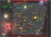 |
Fig. 1 Field of view of the Euclid observations of the ERO Fornax cluster (ERO-F) presented in this paper. North is up and east is to the left. The stack of four VIS images is shown in translucent grey above a colour image from the Fornax Deep Survey (FDS), which shows the brightest cluster galaxy NGC 1399 just off the Euclid pointing in the south-east. The ERO-F field includes ten massive galaxies previously targeted by the ACSFCS (small inset images) around which about 900 GC candidates were identified by that survey (yellow dots: GC probability pGC > 0.95; Jordán et al. 2015). The galaxy FCC161 (NGC1379) is among the galaxies in the ACSFCS survey; however, its final HST data are corrupted. Therefore, no ACSFCS GC catalogue for this galaxy has been published. Additionally, the Euclid FoV overlaps with the position of about 30 dwarf galaxies (large green dots; Venhola et al. 2018, 2022) and about 602 spectroscopically confirmed GCs (red dots; references in the text). |
2.2 Galaxy catalogues
The FoV of ERO-F was chosen to overlap with the location of ten major galaxies (Fig. 1), of which nine have published ACSFCS data2(Jordán et al. 2007, 2015). Additionally, the FoV contains 48 galaxies listed as dwarf or low-surface brightness (LSB) galaxies in the Fornax Deep Survey (FDS) dwarf catalogues (Venhola et al. 2018, 2022). Here, we consider the 45 galaxies with Mr > −17 as dwarf galaxies. The remaining three galaxies in the FDS dwarf catalogue are relatively brighter than the rest of the sample and are among the 10 massive galaxies observed by ACSFCS. After visual inspection of the IE frame, we exclude from further analysis some objects from the FDS list: those that appear to be spiral galaxies; duplicates in the catalogues; and dwarf galaxies that are not fully covered by stacked frames in one of the filters. This selection leads to a sample of 30 dwarf galaxies for further analysis of their GCs. Tables 1 and 2 present the galaxy samples used in this paper. In these tables, properties of galaxies are adopted from Venhola et al. (2018, 2022) and Spavone et al. (2020). The stellar masses of the dwarf galaxies in Table 2 are derived based on equations in Taylor et al. (2011) using the total r-band magnitudes and g − i colours measured by Venhola et al. (2018, 2022).
2.3 GC catalogues
Our searches for GCs in the Fornax cluster take advantage of previous surveys of GCs and compact sources in the cluster, conducted from the ground and from space. ACSFCS (Jordán et al. 2015) used the HST Advanced Camera for Surveys (ACS) to acquire 202″ × 202″ images centred on galaxies within the ERO FoV (Fig. 2). The images were taken in the F475W band with an exposure time of 760 s, and in the F850LP band with a total exposure of 1220s (2 × 565 s + 90s), and have an initial pixel scale of 0′.′05. The ACSFCS team exploited a combination of colour, magnitude, compactness, and distance to the host galaxy centre to identify GC candidates and compute the probability of the candidates being a GC (Jordán et al. 2015; Liu et al. 2019). This probability is larger than 95% for 906 ACSFCS catalogue objects in our field. In the remainder of this paper, we always use this 95% probability cut when exploiting the ACSFCS catalogue. Furthermore, the Fornax cluster has been the target of several spectroscopic surveys and more than 2 800 GCs are spectroscopically confirmed (Hilker et al. 1999; Drinkwater et al. 2000; Mieske et al. 2004; Bergond et al. 2007; Firth et al. 2007, 2008; Gregg et al. 2009; Schuberth et al. 2010; Pota et al. 2018; Fahrion et al. 2020; Chaturvedi et al. 2022)3. About 602 of these GCs overlap with the Euclid observations, of which 225 GCs are in common with the ACSFCS GC catalogue. We use these samples of previously known GCs as a reference set to establish our methodology for GC identification in Sect. 4.
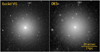 |
Fig. 2 Euclid IE data (two-image stacked frame) versus the Dark Energy Survey (Abbott et al. 2021) in the r band for a cutout around dwarf galaxy FCC188 (FDS11_DWARF155). The galaxy is surrounded by several small point-like sources, some of which are the GCs of the galaxy. Given the high-resolution images of Euclid in IE , we are were to resolve the majority of GCs around similar objects and distinguish them from foreground stars. These images have a total exposure time of 1120 s and 720 s for Euclid VIS and DES, respectively. |
Properties of the ten most massive galaxies located within the footprint of the Euclid ERO-F images.
3 Data processing
Given the small angular sizes of GCs at the distance of the Fornax cluster, and the similarity of their photometric properties to some of the foreground stars and background galaxies, GC detection and identification requires careful analysis of the detected sources4. To do this, firstly, we model the PSF in all bands (Sect. 3.1). Then we perform source detection and photometry to construct a source catalogue (Sect. 3.2). The performance of source detection is then investigated using GC simulations (Sect. 3.3). Subsequently, we examine the photometric properties of the known GCs, namely ACSFCS GC candidates and spectroscopically confirmed GCs (Sect. 4.1). Using the observed properties of known GCs combined with the outcome of the GC simulations, we finally search for GC candidates within the data (Sect. 4.2). GC selection is done using the compactness indices and colours of the sources. The resulting GC sample is used in Sect. 5, where we examine the distribution of intracluster GCs (ICGCs) and GC properties of Fornax cluster dwarf galaxies.
3.1 Point spread function
Point spread function models are constructed from the stacked frames and they are used to estimate aperture corrections (Sect. 3.2) as well as to simulate GC images (Sect. 3.3). One PSF model is produced per filter. For IE, the PSF model is made from the two-image stacked frame. To produce these models for a given filter, an initial catalogue is produced with SExtractor (Bertin & Arnouts 1996) in its default configuration. Subsequently, non−saturated bright points sources are selected based on MAG_AUTO, FWHM_IMAGE, and ELLIPTICITY, as well as the FLAGS parameters of SExtractor. We select objects with 19 < MAG_AUTO < 21 (for the IE PSF model), 18 < MAG_AUTO < 20 (for the YE, JE, and HE PSF models), ELLIPTICITY < 0.1, FLAGS < 4 and a range in FWHM_IMAGE that is determined from the point source sequence in the FWHM_IMAGE–MAG_AUTO diagram of a given filter. Next, cutouts of 40 pixels × 40 pixels (4″ × 4″ in IE and 12″ × 12" in YE, JE, and HE) are made around the selected point sources (about 1000 sources in each filter). We update the centroid of sources by running SExtractor on the cutouts. Subsequently, taking into account the new centroids, all the cutouts are normalised and stacked using SWarp (Bertin et al. 2002). The output of the stacking is the PSF model. The stacking is done with an over-sampling factor of 10 for each filter.
3.2 Source detection and photometry
We now produce a detection frame from the IE image and subsequently measure the photometry of compact sources. We make the detection frame by applying a ring filter with inner and outer radii of 4 and 8 pixels to the data in IE . This procedure subtracts the light of galaxies, which improves the detection of GCs around galaxies using SExtractor, in particular for the most massive galaxies. This step is particularly important because the majority of the known GCs that we target to validate our methodologies are located in such massive galaxies.
For source detection, we run SExtractor on the detection frame. We modify some of the SExtractor parameters and use tophat_1.5_3x3.conv kernel for filtering the stacked frames to maximise point source detection. In total 93 995 and 207 842 sources brighter than IE = 25 and IE = 26, respectively, are present in the final source catalogue. Table 3 summarizes the SExtractor parameters that are used for source detection.
Given the detections in IE from the previous step, we perform (forced) aperture photometry at these positions (now using the aperture task of photutils because this circumvents the need for identical pixel coordinates in all images when using SExtractor). Fluxes are measured within an aperture radius of 1.5 times the FWHM of the PSF for each filter (2.8 pixels in IE, and between 2.4 pixels and 2.8 pixels in YE, JE, and HE). Afterwards, for each source, the background is estimated within an annulus with an inner radius of 5 times the FWHM of the PSF and a thickness of 20 pixels.
We correct the measured aperture magnitudes for the aperture size using the PSF models. Flux corrections are 8% in IE and 5% in YE , JE , and HE stacked frames, consistent with the measurements of Massari et al. (2025). Considering that the majority of the GCs at the distance of the Fornax cluster, though compact, are not strictly speaking point sources in IE , we expect that our aperture-corrected photometry misses a small fraction of the total flux of GCs in that band. We evaluate this fraction for IE (this effect is negligible for the near-infrared bands) by aperture photometry of ACSFCS GC candidates with a diameter of 1.5 times and 20 times the FWHM (2.8 pixels and 40 pixels) and find an average magnitude offset less than 5%. The larger aperture diameter encloses more than 0.998 of the total flux of the PSF (Cuillandre et al. 2025). Additionally, photometry of the artificial GCs injected into the data (Sect. 3.3) shows that for a typical GC with rh = 3 pc, we lose up to 5% of the total flux.
Additionally, we performed aperture photometry within 2, 4, and 8 pixel aperture diameters. We used these aperture magnitudes to set up proxies for source compactness, which allowed us to exploit the spatial resolution of the VIS images when selecting GC candidates. The difference between two aperture magnitudes is a widely used and simple way of characterising the light profile of compact sources in this context (Peng et al. 2011; Powalka et al. 2016; Harris et al. 2020). Here we define two compactness indices in IE , namely C2-4 (for aperture diameters of 2 and 4 pixels) and C4–8 (4 and 8 pixels)5. The first compactness index measures the concentration of the light in the inner parts of light profiles, while the second is sensitive to the outer parts.
SExtractor parameters that were used for making detection frames and source extraction.
3.3 Artificial GCs and expected completeness
We assess the performance of GC detection by injecting artificial GCs into the frames and applying the same source detection and photometry procedure as in Sect. 3.2. The light profiles of the artificial GC images follow King profiles (King 1962), which are characterised by a core radius rc , a tidal radius rt and a concentration index log10(rt/rc). We set the latter to 1.4, a central value in the range 0.5–2.4 that is observed for Milky Way GCs (Harris 1996).
We vary the half-light radii rh between 2 pc and 6 pc (0.8 ⩽ rc/pc ⩽ 2.4), and the absolute IE magnitudes between −11 and −5, and we set the colours to IE − YE = 0.45, IE − JE = 0.45, and IE − HE = 0.45 (see Appendix B and Euclid Collaboration: Voggel et al., in prep. for typical spectral energy distributions of GCs over the spectral range relevant to Euclid). Each King model is then convolved with the PSF. At the end, Poisson noise is added to the artifical GCs. We produce 3000 artificial GCs in total, making sure to avoid placing them inside the image gaps. We then run the detection and measurement pipeline of Sect. 3.2 on the new images. Since that carries out forced photometry in the NISP bands at the position of the IE detections, we declare a GC detected in one of the infrared bands if the difference between input and output magnitude is smaller than 1.0.
We show in Fig. 3 that the IE , YE , JE , and HE detections are 80% (50%) complete down to magnitudes 26.2 (26.5), 24.0 (25.3), 24.0 (25.4), and 23.6 (25.5), respectively. The 50% and 80% detection-completeness magnitudes were estimated by fitting a modified version of the interpolation function of Fleming et al. 1995:
![Mathematical equation: $f(m) = {1 \over 2}\left[ {{c_0} - {{\alpha \left( {m - {m_0}} \right)} \over {\sqrt {1 + {\alpha ^2}{{\left( {m - {m_0}} \right)}^2}} }}} \right],$](/articles/aa/full_html/2025/05/aa50784-24/aa50784-24-eq1.png) (1)
(1)
where c0 is an additional free parameter compared to the original equation that corresponds to the completeness at the brightest magnitude. The IE − YE colour is used later for GC identification. When both IE and YE detections are required, we expect a completeness of about 80% (50%) for objects brighter than IE = 25.2 (26.2). These magnitudes are about 1.7 and 2.7 fainter than the typical turn-over magnitude of the GCLF, located at IE = 23.5 (i.e. MV = −7.5 with V − IE = 0.5, as described in Sect. 4.2).
4 Selection of GC candidates
Our selection of GCs among all the detected sources is based on the properties of previously known GCs (Sect. 2.3), and on the characteristics of the simulated GCs (Sect. 3.3). Here we first examine the characteristics of the known GCs in the IE stacked frame before defining a selection procedure.
4.1 Compactness of the known GCs and of simulated GCs
The top panel of Fig. 4 shows the compactness indices measured for the two reference sets of known GCs in the 2-image VIS stacked frame. We match catalogues using a cross-match radius of 0′.′5. In the ACSFCS catalogue, we consider only the objects with a GC probability (PGC) larger than 0.95. The scatter in compactness originates from the natural range of sizes of globular clusters, combined with noise that mainly affects the candidates located very close to their host galaxy (closer than 30″), for which the photometry is affected by the light of their host galaxies.
The compactness indices of the simulated clusters are displayed in the middle panel of Fig. 4. For index C2−4 (left panel), the dispersion in the empirical stellar sequence is larger than the dispersion among artificial clusters with small radii. The simulated GCs are injected in the stacked frame rather than into raw frames, with a single PSF model; hence the point source scatter shows that much of the dispersion in the empirical C2-4 is likely due to source-to-source variations of the core of the PSF in our two-image stacks, themselves resulting from a combination of intrinsic effects (spatial and colour-dependent variations of the PSF in the raw frames and changes in the PSF between the two combined exposures), effects of interpolation during the astrometric transformation, and possible weighting effects while stacking. All these effects are not typical of the EWS, and developing more detailed specific software for one particular non-standard image set was deemed too costly. The middle row of Fig. 4 nevertheless indicates the expected location of clusters and shows that our reference samples (top panels), both spectroscopically confirmed and from ACSFCS, mostly contain objects with half-light radii smaller than about 5 pc, with a sparsely populated tail to larger values.
From Fig. 4 (upper panel) we see that the majority of the known GCs have a larger compactness index than the vertical sequence of point sources. This is clear in particular for C2-4 . Point sources have average C2−4 and C4−8 values of 0.70 and 0.26. The majority of known GCs have C2−4 in the range of 0.7–1.0, and C4−8 between 0.2 and 0.5 This range of compactness is also consistent with the outcome of the GC simulation, as is shown in the middle panels of Fig. 4. Based on this figure, objects with C2−4 > 0.8 are resolved. This compactness threshold corresponds to a GC half-light radius of 2.5 pc measured by ACSFCS.
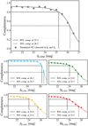 |
Fig. 3 Completeness expected in the ERO-Fornax catalogue data based on artificial GCs. Top panel: combined completeness for sources detected in both IE and YE as a function of simulated input IE magnitude. Bottom: detection completeness in the four individual filters as a function of the respective input magnitude. For old GCs (older than 7 Gyr) with sub-solar metallicities (Z < 0.02), the GCLF turn-over magnitude is expected to be at IE = 23.5. |
4.2 GC identification
We identify candidate GCs in the source catalogue in two steps, the first based on the compactness indices, and the second on colour. In the first step, we select marginally resolved sources by requesting compactness indices that are broadly within the range expected from known GCs and simulations. We select sources with compactness indices within 99% quantile from the median value of C2−4 and C4−8 in a given magnitude range for the artificial GCs. Additionally, to take into account any other effects in GC compactness not included in the simulations (see Sect. 4.1), we extend the upper limits on compactness by 0.1 mag. This value corresponds to half of the width of the stellar sequence in C2−4 . The resulting sample, after applying the compactness criteria, is shown in the lowest panels of Fig. 4. This selection picks up more than 80% of the spectroscopic GCs, as well as the GC candidates in the ACSFCS catalogue. The majority of the remaining 20% of GCs are objects that are in close vicinity to the bright galaxies, and therefore their photometry is strongly affected by the galaxy. This effect is stronger for fainter GCs. Selection in this step includes 17 596 sources brighter than IE = 25 out of the initial 93 995 sources (18.7%).
Subsequently, in the second step of GC identification, we apply colour cuts to the initial GC sample. The range for these colour cuts is determined using the observed colours of known GCs in the ERO-F data, as shown in Fig. 5. With colour selection, we mainly aim to clean the initial GC sample from background galaxies and artefacts. Figure 6 shows the IE − YE colour of GCs, as well as foreground stars and background galaxies in the ERO-F. The stars and galaxies are selected based on their radial velocities (Maddox et al. 2019; Saifollahi et al. 2021a). The background galaxies have IE − YE > 0.8 while GCs have IE − YE < 0.8. Therefore, we selected objects with IE − YE bluer than 0.8. We also apply a lower limit at IE − YE = 0 given the colours of the known GCs in Fig. 6. The colour-colour diagrams show that the known GCs and foreground stars have similar IE − YE colour, and therefore a careful GC selection based on the compactness of sources is essential (previous step). In addition to the IE − YE colour cut, we apply YE − JE and JE − HE colour cuts. Here we aim to increase the purity of the sample while retaining as much completeness as possible. Therefore, we applied these colour cuts (YE − JE and JE − HE ) to objects with positive flux (from forced photometry at fixed positions) in JE and HE . This means that we keep sources without detection in JE or HE . The colour-ranges in YE − JE and JE − HE are between −0.3 and 0.5 (for both colours). These are conservative cuts considering the range of actual GC colours, based on synthetic photometry of star cluster models (cf. Appendix B). These models show that GCs with old stellar populations (older than 7 Gyr) and sub-solar metallicities (Z < 0.02) have Euclid colours 0.2 < IE − YE < 0.8, 0.05 < YE − JE < 0.24, and −0.12 < Je − He < 0.16. In addition to the colour cuts, here we only include sources with ELLIPTICITY smaller than 0.5 (in IE) as GC candidates. This is the observed upper limit for the known GCs as well as the artificial GCs. The procedure described above results in 5449 GC candidates as faint as IE = 25, out of the 17 241 sources in the initial GC sample (31.6%).
When it comes to GC selection, there is always a trade-off between the completeness and purity (cleanness) of the final GC sample. The above-mentioned limits on colours are strict and are applied in order to have a clean GC catalogue. However, for identifying GCs around dwarfs, a more complete sample is desired. Therefore, for selecting GCs of dwarf galaxies we extend the colour range to take into account the scatter from photometric uncertainties, in particular for the fainter GCs. We select sources with IE − YE < 1.2 with no lower limit, and YE − JE and YE − JE between −1.0 and 1.0.
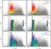 |
Fig. 4 Compactness indices measured in IE and first step of the GC selection. The sources in the full catalogue are displayed in grey. Top panels: compactness indices of the spectroscopically confirmed GCs (red points), and of GCs in the ACSFCS catalogue (yellow points). These two samples serve as empirical references. The vertical sequences at C2−4 = 0.70 and C4−8 = 0.26 correspond to point sources. Objects on the right side of this sequence with a larger compactness index are extended sources. Objects with smaller compactness index are mostly artefacts (e.g. cosmic rays) in the data. Middle panels: Compactness indices of the 3000 artificial GCs with half-light radii between 2 and 6 pc, which were injected into the images (black points). Lower panels: compactness indices of the sources in the initial GC sample after selection based on their compactness indices, as described in Sect. 4.2 (green points). The colours in these panels demonstrate source density in the parameter space. |
5 Results
In the previous section, we performed source detection and photometry, produced multi-wavelength source catalogues, and selected GCs based on their compactness, colours, and ellipticity. Here, we assess the performance of our methodology and the completeness of the GC selection based on archival GC catalogues. Then, we investigate the properties of GCs within the Fornax cluster and around its dwarf galaxies.
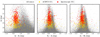 |
Fig. 5 Colour-magnitude diagram of the detected sources (grey points) versus the spectroscopically confirmed GCs (red points) and GCs in the ACSFCS catalogue (yellow points). Considering the photometric uncertainties of the fainter GCs (fainter than IE = 22), the majority of the known GCs have 0.0 < IE − YE < 0.8, −0.3 < YE − JE < 0.5, and −0.3 < JE − HE < 0.5. In this work, we use these colour ranges and apply a colour cut for GC selection. |
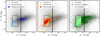 |
Fig. 6 Three panels showing the Euclid colour-colour diagram with (IE − YE) plotted against the (IE − HE) colour index. In each panel, the grey dots show the distribution of all photometric sources. In the left panel, we show the location of foreground stars and background galaxies in cyan and blue, respectively. The middle panels show spectroscopically confirmed GCs as red points, and GCs in the ACSFCS catalogue as yellow points. In the third panel, we show the initial GC candidates as dark green points and the retained GC candidates in light green colours. The applied colour cuts are shown as a dashed box. These colour cuts are used to identify the intracluster GC candidates in the ERO-F data. However, we use a more relaxed colour cut for identifying GC candidates around dwarf galaxies. For that, we apply an upper limit in IE−YE , shown by the vertical solid black line. |
5.1 The Euclid GC sample compared to archive samples
We compare our own source catalogues and GC (candidate) catalogues with the existing ACSFCS and spectroscopically confirmed GC catalogues (Sect. 2.3). For simplicity, we refer to the objects in these reference sets as known GCs. Our first aim is to estimate the completeness of our sample relative to the reference sets. There are 602 spectroscopically confirmed GCs in the FoV of our observations, out of which 600 (more than 99.5%) are initially detected by SExtractor in IE. In the case of the ACSFCS GC candidates, 906 candidates overlap with the data, of which 888 (98%) are detected. This is consistent with the expectations from the completeness assessment based on artificial GCs. As seen in Fig. 3, GC detection in IE is more than 95% complete by magnitude IE = 25.0. GC selection based on compactness indices retains 80% of the known GC sample. About half of the non-selected GCs are close to the centres of major galaxies, within about 30 arcsec (2.9 kpc), in regions where the light of the bright galaxies affects their photometric properties.
When adding the cuts in colour space to our GC selection we find that our completeness decreases. Our colour selection includes only the main locus of the GC colours (see middle panel of Fig. 6), and we have traded completeness for higher purity. Here we identify 70% of the known GCs, including ACSFCS GC candidates and spectroscopically confirmed GCs, farther than 90 arcsec from the massive galaxies. This rate is expected to be valid elsewhere in the data, within the cluster. This rate is about 80% for dwarf galaxies considering the less strict colour cut applied for GC selection around them. This is consistent with the estimated completeness of combined IE and YE detections from GC simulations; that GC detection rate is 80% down to IE = 25.2, which is 1.7 mag fainter than the typical turn-over magnitude of GCLF. After applying colour cuts, we identify 5631 and 1923 GC candidates in the Fornax cluster brighter than IE = 25 and IE = 23.5 (the typical GCLF turn-over magnitude), respectively, of which 4691 and 1556 are not in any of the previous spectroscopic catalogues and the ACSFCS candidates (with high GC probability).
The purity of the final GC sample is harder to evaluate. Normally, the purity of a photometric GC sample can be evaluated by comparing the sample with a complete sample of spectroscopically confirmed GCs and/or assessing the identified GC candidates in a field where no GCs are expected. Neither of these two approaches applies to the ERO-F given the incomplete spectroscopic GC samples and the high GC density environments in the central region of the Fornax cluster. Instead, we employ the uiKs diagram (u − i versus i − Ks) to make an assessment of the GC candidates, assuming that the true GCs lie on a specific GC sequence in this colour-colour space (Muñoz et al. 2014). For this purpose, we cross-match the GC candidates with the optical/near-infrared photometry of the Fornax cluster provided in Saifollahi et al. (2021a). Given the limited depth of the ground-based data in u and Ks , we can only assess GC candidates brighter than IE = 21.5 with this method. In this magnitude range, 90% of the candidates have photometry in u and Ks . The upper panel of Fig. 7 shows the uiKs diagram for the detected sources in the data, including spectroscopic GCs, spectroscopic stars and galaxies, as well as the GC candidates in this work. By visually assessing this plot, more than 90% of the GC candidates seem to be located on the GC sequence, while less than 10% are consistent with being foreground stars and background galaxies, respectively.
While the uiKs diagram is powerful in distinguishing GCs and non-GCs, collecting sufficiently deep (ground-based) data in u and Ks is very challenging and observationally expensive. In the meantime, the gri colour-colour diagram (g − r vs. r − i), even though it does not provide a clear separation between GCs and non-GCs (Fig. 7 in the lower panel), can be assessed for GCs 2 mag fainter than what is shown in the uiKs diagram. Here we do not apply any colour cuts based on the ground-based optical/near-infrared photometry; however, these additional photometric data from deep ground-based surveys (e.g. FDS, DES, NGFS for the Fornax cluster) are complementary to Euclid data and could be used in future for further cleaning the GC samples. For the EWS, the data from Euclid ground segment will provide complementary deep optical imaging data. In particular, the Canada–France Imaging Survey (CFIS) and the Legacy Survey of Space and Time (LSST) data in u-band will be beneficial for further cleaning the catalogues of GC candidates derived from Euclid observations from non-GCs.
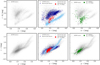 |
Fig. 7 Colour-colour diagrams showing uiKs (upper panel) and gri (lower panel) for the detected sources in ERO-F data (grey points), using the photometry of the Fornax Deep Survey (FDS, Peletier et al. 2020) provided in Saifollahi et al. (2021a). GCs (red points) are known to show a well-defined sequence in uiKs separated from stars, except those at the bluest end (light blue points), and from galaxies (dark blue points). More than 90% of the bright GC candidates with IE < 21.5 (green points) selected in this work are located on this diagram, while less than 10% are consistent with being a foreground star or background galaxy. |
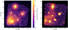 |
Fig. 8 Projected distribution and density map of GC candidates (white points) brighter than IE = 23.5 (left panel) versus the diffuse light in IE (background image in the right panel) in the ERO-F field of view in the Fornax cluster. In the left panel, the size of the white points (GC candidates) corresponds to the total magnitude of GC candidates (brighter GCs appear larger). In the right panel, the smoothed version of the ERO-F data made from four exposures is shown. This is a different stack than the stacked frame used for the GC selection (which is made from two exposures with the best PSF). The black lines within the image are regions without any available data. |
5.2 The spatial distribution of GCs
Due to the magnitude limits of the spectroscopic searches for GCs in the Fornax cluster, such surveys have only covered the brightest end of the GCLF and are highly incomplete at the faint end. The ACSFCS survey is deep but limited to small fields around the galaxies in their sample. Therefore, the distribution of the intracluster GCs (ICGCs) is less known outside the core of the Fornax cluster. On larger spatial scales, the most recent ground-based photometric searches of GCs within the virial radius of the cluster (Cantiello et al. 2020; Saifollahi et al. 2021a) are expected to be contaminated by non-GCs, as discussed in the previous subsection. In the Euclid data, we automatically identify GC candidates independent of their location and thus also in the intra-cluster region. Since our sample is expected to be about 70% complete, we can examine the spatial distribution of intra-cluster GCs.
Figure 8 shows the projected distribution and the density contours of the selected GCs brighter than IE = 23.5 across the FoV in the left-hand panel. In the right-hand panel, the four-image IE stacked frame is shown. In this frame, the main galaxies and extended diffuse intracluster light (ICL)6 within the Fornax cluster can be easily seen. At first glance when considering Fig. 8, the density distribution of the GCs appears to share some patterns with the ICL. In particular, it seems that both the GC distribution and the ICL show a characteristic excess in the south-east corner of the FoV, which is expected because this is the direction of FCC 213 (NGC 1399), the central dominant galaxy of the Fornax cluster that is located just outside the field of view (D’brusco et al. 2016; Cantiello et al. 2020; Diego et al. 2023). Here, we discuss and investigate this possible connection between the ICL and the GC density distribution in more depth.
5.2.1 Intracluster light within the Fornax cluster
The apparent distribution of the diffuse light in the ERO-F data must be interpreted with caution because of low-level straylight in some areas of the ERO-F image. Iodice et al. (2016) used FDS deep images to highlight the extended diffuse halo of FCC 213, the western part of which is also clearly seen in the south-east corner of our FoV. Iodice et al. (2017) subtracted galaxy light and they were able to describe a much more extended diffuselight distribution, which reaches (in projection) from FCC 213 to FCC 184 and to the smaller elliptical galaxy FCC 182, and even to the edge-on spiral FCC 170. The 4-image IE stack from ERO-F confirms the presence of diffuse light on these scales. The diffuse light is clearly significant from FCC 213 to FCC 184 and FCC 167, but only marginally significant north of FCC 170. Future EWS data, in which a correction for straylight in IE will be implemented that is not yet available, will be needed to check whether or not diffuse light really extends from the central regions of the galaxy cluster to FCC 167 in the north of our FoV or to FCC 147 towards the west. Such extensions are not seen in the ground-based data of Iodice et al. (2017), but a connection to FCC 167 would not be too surprising considering the current understanding of the three-dimensional structure of this area of the Fornax cluster. Indeed, according to the surface brightness fluctuation (SBF) estimates of Blakeslee et al. (2009), recalled in Table 1, FCC 213 and FCC 167 are at similar distances, respectively, (20.9 ± 0.9) Mpc and (21.2 ± 0.7) Mpc. The projected separation between these two galaxies is only about 250 kpc. On the contrary, Blakeslee et al. (2009) place the spiral FCC 170 about 1 Mpc further (21.9 Mpc), and FCC 147 about 1 Mpc closer to us (19.6 Mpc).
5.2.2 Distribution of GCs versus ICL
To further investigate this possible connection between the ICL and the GC density, we divide the FoV of the ERO-F data into a 20 × 20 grid and calculate the GC density, the average ICL flux density, and the ratio between these two in each cell. This is shown in Fig. 9. To calculate the ICL flux density, we mask the pixels in the image above a threshold that corresponds to roughly 4 times the half-light radius for the bright galaxies. This is necessary so that the calculation of the average flux is not dominated by bright galaxies and stars in the cells. As seen in Fig. 9, the area around the brightest galaxies in the FoV produces several local peaks in both GC density and ICL flux maps. Outside the proximity of the bright galaxies, we see substantial ICL flux, as well as GC density. To calculate the ratio between GC density and ICL flux density, we use the same mask used earlier. As shown in Fig. 9c, the ratio between GC density and ICL flux scatters around the mean and there are no areas with obvious lack of GCs compared to what would be expected from the ICL, indicating that the ICL mostly follows the GC distribution.
This correlation between the ICL flux density and GC density is visualised in Fig. 10 for each cell of the two-dimensional histogram. We find a correlation between the average ICL flux density and GC density indicating that indeed most of the GCs follow the ICL distribution. The empty area in the top left of the figure implies that for a given density of GCs, there is always a minimum flux in ICL light that is significantly above the background. This implies that for a certain threshold in GC density, there is always a corresponding minimum diffuse light level, supporting the idea that this correlation is real and not an artefact (e.g. stray light).
Thus, while there is a scatter in the relation, as it is expected, the ERO-F data indicates that GCs trace the ICL light in galaxy clusters. A more global correlation between diffuse light and the density distribution of GCs was also found in ultra-deep JWST observations of a massive cluster at ɀ = 0.4 (Diego et al. 2023; Martis et al. 2024), and in the Euclid observations of the Perseus galaxy cluster (Kluge et al. 2025). A combined view of GCs and ICL within the Fornax cluster emphasizes Euclid’s excellent view of the compact sources and low-surface brightness features at 20 Mpc, despite the non-optimal data used in this work.
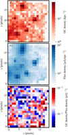 |
Fig. 9 2D maps of GC density, flux density, and the ratio between them across the FoV: (a) GC density in the Fornax FoV binned into a 20 × 20 grid, (b) flux density of diffuse light within the same cells as panel (a), with all bright galaxies and other bright sources masked, (c) ratio between the GC density and the flux density of the diffuse light. The colour-bar on the left corresponds to the ratios shown in this panel. |
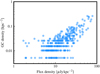 |
Fig. 10 Diffuse light flux density (Fig. 9b) plotted against the GC density (Fig. 9a) for each bin of the 2D histogram. |
5.3 GC properties of dwarf galaxies
The dwarf galaxies we study here (30 galaxies) were taken from the FDS dwarf catalogue (Venhola et al. 2018, 2022), where the authors apply size and colour criteria for discerning member dwarf galaxies from background galaxies. We present the list of these dwarf galaxies and their properties in Table 2. The results of exhaustive searches for new dwarf galaxies in the ERO-F data will be discussed elsewhere. Preliminary tests on these dwarf galaxies have shown that we can use the SBF method to estimate distances for the galaxies in the field, including several dwarfs. This will provide a great tool to establish group membership of the dwarf galaxies in the future.
In Sect. 5.1, we discussed that the GC sample of dwarf galaxies in the ERO-F FoV is expected to be 80% complete. Our sample, unlike the majority of previous works, extends to GCs well below the GCLF turn-over magnitude. However, at those faint limits, the contribution from intracluster GCs, as well as contamination (foreground stars and background galaxies) become increasingly important, which one must carefully take into account. Figures 11 and C.1 show the brightest dwarf galaxies in the sample and their GCs identified in this work. By visual inspection of the IE images of the dwarf sample, it seems that the dwarf galaxies with a stellar mass less than M* = 107 M⊙, on average host no GCs, although with a few exceptions (Fig. C.2).
Our search for GCs around dwarf galaxies in the ERO-F data also identifies the nuclear star clusters (NSCs, Turner et al. 2012) of several dwarf galaxies in the sample as GC candidates. This is reasonable, given the similarity of the majority of NSCs of dwarf galaxies to bright GCs, in terms of compactness and colours. The suggested formation scenario of NSCs in dwarf galaxies is that NSCs are formed after inspiraling into the centres of galaxies (Ordenes-Briceño et al. 2018; Sánchez-Janssen et al. 2019; Johnston et al. 2020; Fahrion et al. 2022; Román et al. 2023). We find that 47% of all the dwarf galaxies in this study host an NSC, which is consistent with predictions for the nucleation fraction at that mass range (Sánchez-Janssen et al. 2019). Furthermore, for four dwarf galaxies in the sample, we identify a previously undetected NSC, namely galaxies FDS11_365, FDS10_034, FDS16_172, and FDSLSB220. This proves the capabilities of Euclid for detecting the faintest NSCs, which is necessary for studying the nucleation fraction of dwarf galaxies. Considering the newly discovered NSCs, we find a nucleation fraction of 85% for galaxies with a stellar mass between M* = 107 M⊙ and M* = 108 M⊙ (13 galaxies), which is higher than the expected range (50–60%, Sánchez-Janssen et al. 2019). The NSCs of dwarf galaxies will be studied in detail in a future paper (Fig. 12).
In this section, we focus on the properties of GCs around these dwarf galaxies. The intracluster GC candidates are a major source of contamination when studying GCs of dwarf galaxies since there is no way for us to determine whether the candidates of a given dwarf are bound to it. Because our observations are close to the core of the cluster, the density of intra-cluster GCs relative to the GCs of dwarf galaxies is high. Due to this and the fact that dwarfs host a small number of GCs, we use the stacked average properties of GCs around these dwarf galaxies in order to be less affected by individual contamination.
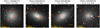 |
Fig. 11 A few examples of Euclid VIS image cutouts centred on the most massive dwarf galaxies in the Fornax cluster in our sample, with stellar masses of M* > 107 M⊙ (see all 14 dwarf galaxies in this stellar mass range in Fig. C.1). The cutouts correspond to 4 times the half-light radius (of dwarf galaxies) on each side. North is up, east to the left. The red circles mark the final GC candidates that were selected based on their compactness and colours. Those candidates that pass the compactness criteria, but do not satisfy colour selection, are shown with orange circles. The green circles show all the sources identified around these dwarf galaxies. The three numbers below the name of each dwarf galaxy correspond to the number of GC candidates within 3Re, the number of GC candidates in the background normalised to the area within 3Re , and the estimated number of GCs corrected for incompleteness, respectively. |
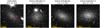 |
Fig. 12 Similar to Fig. 11 but for dwarf galaxies with stellar mass M* < 107 M⊙ (see all 16 dwarf galaxies in this stellar mass range in Fig. C.2). On average, the galaxies in this stellar mass range do not host GCs; however, there are a few exceptions with GC number counts greater than zero. Considering the detections and possible contaminants, statistically one expects the dwarf galaxies FDSLSB45 (with M* = 5.89 × 10⁵ M⊙), FDSLSB43 (with M* = 5.83 × 10⁵ M⊙), FDS16_DWARF227 (with M* = 5.78 × 10⁵ M⊙), and FDSLSB36 (with M* = 5.76 × 10⁵ Mo) with 1.0, 0.7, 0.9, and 0.7 GCs, respectively (see Fig. C.2). |
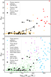 |
Fig. 13 Total number of GCs as a function of the stellar mass of the host for the dwarf galaxies in this work (black stars). Top: Comparison with other studies in the Fornax cluster. The total GC numbers of massive galaxies from ACSFCS from Liu et al. (2019) are shown as red discs and those of the Fornax cluster central LSB galaxies from Prole et al. (2018) as yellow crosses. The black curve shows the average GC number for a given mass range of dwarf galaxies in this work (30 galaxies). Error bars correspond to the uncertainties on the mean. The three relatively GC-rich dwarf galaxies above this curve are indicated by the last three digits of their FDS name. Bottom: GC numbers for galaxies in other environments. Massive galaxies from the ACS Virgo Cluster Survey (Peng et al. 2008) are shown as blue squares, Virgo cluster dwarf galaxies from Carleton et al. (2021) as green triangles, dwarf galaxies in the local Volume from Carlsten et al. (2022) as green crosses, NGC5846-UDG1/MATLAS2019 from Müller et al. (2021) with a purple disc (the value of 54 GCs reported by Danieli et al. 2022 for this galaxy is beyond the range displayed), UDGs from Saifollahi et al. (2022) and Ferré-Mateu et al. (2023) (see references therein) as pink squares, and NGC1052 DF2 and DF4 from Shen et al. (2021) as dark blue triangles. |
5.3.1 Total GC number
The GC numbers are estimated by counting all the GC candidates as faint as IE = 25.0 within a 480 arcsec box around each galaxy. We count the GC candidates within 3Re (dwarf-GC count), and between 5Re and 15Re (background count), and normalize the counts to the area within 3Re. Then, we subtract the latter from the former and correct the result for incompleteness (a factor of 1.25, considering the overall completeness of 80% in GC identification), which then gives us an estimate of the total number of GCs (NGC). We note that this is different from the approach taken in the majority of recent works on GCs of dwarf galaxies that count GCs up to the turn-over magnitude of GCLF and correct the GC total number for the faint end of the GCLF (a factor of 2). Instead, we count all the GCs, considering that our observations are expected to reach the faint end of GCLF. Additionally, we justify the choice of 3Re later in this section, where we study the radial distribution of GCs around their host dwarf galaxies. This choice is consistent with the GC radial distribution previously observed for dwarf galaxies (Carlsten et al. 2022). Ideally, one needs to study the GCLF and the GC distribution of individual objects to estimate the GC number. However, this is not possible for low GC count objects such as the dwarf galaxies in our sample.
The total number of GCs in a given galaxy correlates with its total dark matter halo mass (Harris et al. 2013; Burkert & Forbes 2020) as a consequence of the hierarchical formation of massive galaxies (El-Badry et al. 2019). However, for dwarf galaxies, while the observational evidence supports such a correlation, more studies are needed to understand the physics behind this scaling relation. We present the total number of GCs for a given galaxy in Fig. 13. For dwarf galaxies less massive than M* = 107 M⊙, the average number of GCs per galaxy is consistent with zero, except in a few cases. In particular, for a few dwarf galaxies with a stellar mass of less than M* = 106 M⊙, namely FDSLSB45 (with M* = 5.89 × 10⁵ M⊙), FDSLSB43 (with M* = 5.83 × 10⁵ M⊙), FDS16_DWARF227 (with M* = 5.78 × 10⁵ M⊙), and FDSLSB36 (with M* = 5.76 × 10⁵ M⊙) with 1.0, 0.7, 0.9, and 0.7 GCs, respectively. The dwarf galaxies with a stellar mass larger than M* = 107 M⊙ host between 0 and 13 GCs, while 17% of them have a GC number of 5 and more.
Figure 13 compares the total GC numbers of dwarf galaxies in this work with the ones in the literature in the Fornax cluster (upper panel) and in other environments (lower panel). The upper panel of Fig. 13 presents the total GC numbers of Liu et al. (2019) for the massive galaxies in Fornax using the ACSFCS observations, and those of Prole et al. (2019) for LSB galaxies in the central regions of Fornax using the data of FDS. We also present the average GC number of dwarf galaxies in this work for four stellar mass bins (black curve). Overall, the GC numbers of galaxies seem to follow a continuous relation from the massive galaxies (red circles) to dwarf galaxies (back stars). Some of the dwarf galaxies show a higher than average GC number, namely FDS16_DWARF257, FDS11_DWARF294, and FDS11_DWARF306 with estimated GC numbers of 12.2, 13.0 and 11.1 (background-subtracted and completeness-corrected). These GC-rich dwarf galaxies are indicated in the upper panel of Fig. 13 and are located above the black curve.
In the lower panel of Fig. 13, along with the total GC numbers in this work, we present the GC numbers of the massive (Peng et al. 2008) and dwarf galaxies (Carlsten et al. 2022) of the Virgo cluster, and of local Volume dwarf galaxies (Carlsten et al. 2022). In addition to these GC samples, we show the results for some GC-rich ultra-diffuse galaxies (UDGs, van Dokkum et al. 2015) in the literature studied using HST Saifollahi et al. 2022; Ferré-Mateu et al. 2023; Gannon et al. 20247. Here we use the GC numbers from the catalogue, except the GC numbers of some of the Coma cluster UDGs DF44, DFX1, DF07, and DF17. For these Coma cluster UDGs, we use the more recent GC number estimates in Saifollahi et al. (2022). We also included NGC 5846-UDG1/MATLAS2019 in the NGC 5846 group (Müller et al. 2021; Danieli et al. 2022), and NGC 1052-DF2 and NGC 1052-DF4, two UDGs lacking dark matter in the NGC 1052 group (van Dokkum et al. 2018b, 2019). In this context, The GC numbers of the three GC- rich dwarf galaxies (FDS16_DWARF257, FDS11_DWARF294, FDS11_DWARF306) seem to be an extension of the GC-rich UDGs with two to three times more GCs than average at a given stellar mass. These dwarf galaxies are a UDG by definition (FDS11_DWARF306 with Re = 1.45 kpc is marginally a UDG). The galaxy FDS11_DWARF246 is another UDG in the sample with zero GCs. This dwarf galaxy is located close to the FCC 213, and therefore the estimated GC number for this object is highly affected by the ICGS. In the future, with such information on the GC contents of dwarf galaxies as well as their stellar populations, we will be able to investigate the various formation scenarios of UDGs and dwarf galaxies (Ferré-Mateu et al. 2023; Buzzo et al. 2024). The latter would be possible using Euclid’s data combined with the ground-based surveys.
5.3.2 GC luminosity function
The GCLF of massive galaxies typically follows a near-Gaussian profile in logarithmic units of luminosity with a peak around MV = −7.5 (Rejkuba 2012) and a standard deviation of σ = 1.2 mag. Trends with host galaxy properties have been identified, such as a decrease in the width of the GCLF with decreasing luminosity (Villegas et al. 2010, hereafter V+10). The study of the GCLF of low-mass dwarf galaxies requires larger galaxy numbers than for massive galaxies, and the GCLF properties in this regime remain controversial. While earlier works showed that the GCLF is Gaussian for dwarf galaxies (Georgiev et al. 2009), more recent work on UDG and LSB galaxies has suggested that there might be a wide range of GCLFs for dwarf galaxies (van Dokkum et al. 2018a). This could be a consequence of small galaxy samples, as well as small numbers of GCs within dwarf galaxies, or bias towards the environment with the FoV. With a single Euclid pointing within the Fornax galaxy cluster, small samples remain a limitation for the dwarf galaxy GCLF and the early trends discussed must be reviewed when full coverage becomes available.
Before producing the GCLF, we repeat the photometry of GC candidates in IE using an aperture with a radius of 3 times the FWHM in IE, about 5.7 pixels. This aperture is twice the size of the aperture used in Sect. 3.2 and provides a better estimate of the total luminosity of the GCs. This choice of aperture size is particularly important for studying the GCLF at the bright side, where GCs are typically larger. For these GCs, our earlier photometry with smaller apertures would underestimate their total luminosity by about 10% for the largest GCs, while with the larger aperture, the fraction of missing light is below 1%. Using a smaller aperture for photometry of GCs would lead to more accurate magnitude and colour estimates for fainter and smaller GCs, which is critical for GC identification and that is why it was used earlier in Sect. 3.2.
Here, we produce the GCLF using all GC candidates within 4 Re of their host for massive galaxies (in Table 1), and within 2 Re for dwarf galaxies. We exclude the central 0.1 Re of dwarf galaxies to remove the NSCs, and the central 0.2 Re of massive galaxies where GC selection becomes too difficult. The different selection radii are implemented because the radial extent of GC systems relative to the effective radius of their host is known to scale with the host galaxy mass (De Bórtoli et al. 2022), and because a selection radius larger than 2 Re for dwarfs is not warranted by our data (see Sect. 5.3.3). For massive galaxies, our selection radius is about 15% larger than the typical effective radius of the GC systems found by Hudson & Robison (2018).
The stacked GCLF of dwarf galaxies includes dwarf galaxies with a stellar mass larger than M* = 107 M⊙ (14 dwarf galaxies, shown in Fig. 11), which have GC numbers larger than 1. We sum up all the GC candidates for these 14 dwarf galaxies and derive the stacked luminosity function of GC candidates of dwarf galaxies. Next, we estimate the average contamination from the background and subtract it from the luminosity function of GC candidates. The background includes intracluster GCs, as well as any foreground stars or background galaxies that passed the GC selection criteria. We estimate its contribution by selecting GC candidates between 5Re and 15Re from the 14 dwarf galaxies used for this analysis, normalised to the total area of the background and multiplied by the total area within 2 Re of the 14 dwarf galaxies. Finally, we correct the background-subtracted luminosity function for the incompleteness of detection, based on the results of Sect. 3.3. We use the same background and completeness correction procedure for deriving the GCLF of massive galaxies. The outcome is the stacked GCLF of galaxies shown in Fig. 14. For the massive galaxies (top panel), we do indeed recover a GCLF similar to a Gaussian for our GC candidates. It has a turnover at IE = 22.90 ± 0.09, which corresponds to an IE absolute magnitude of −8.59 ± 0.09. A conversion between IE and V for old and metal-poor GCs leads to MV = −8.06 mag. The width of the GCLF is σ = 1.06 ± 0.07. The derived GCLF parameters are consistent with the GCLF parameters reported in V+10 using the ACSFCS data.
The GCLF of dwarf galaxies is shown in the bottom panel of Fig. 14. Its appearance is more irregular than that of the massive galaxies; despite stacking we remain in a regime of small number statistics with this single-field observation. The initial dwarf GC-candidate sample contains 112 objects, and we distributed them into 12 bins. After statistical correction for the background, this number is reduced to about 38 objects. The statistical errors are estimated with Poisson statistics before background subtraction and then propagated. We have obtained best-fit Gaussian estimates of the intrinsic GCLF of dwarf galaxies in two ways. Firstly, we computed heteroscedastic maximum-likelihood parameters for the binned background-corrected distribution (Fig. 14). Secondly, we computed parameters using individual measurements (before any background subtraction), for a model that combines a representation of the background magnitude distribution, a Gaussian GCLF for the dwarfs, the completeness correction, and a prior on the proportion of contaminants that is compatible with the statistical background subtraction of the first method. In the second approach, the parameters are the mean and standard deviation of the Gaussian and the relative scaling of the Gaussian relative to the background. This latter method takes into account the individual photometric uncertainties. Details for it are provided in Appendix A. Both methods can be repeated, with variations for instance in the exact bin boundaries for the first one, or in the exact range of magnitudes taken into account for the second.
Using the first method, we find that the best-fit Gaussians have a mean magnitude of µpeak = 23.6 ± 0.42, and a GCLF width of σ = 1.00 ± 0.33. The second method based on individual measurements gives µpeak = 23.2 ± 0.2, and a GCLF width of σ = 0.9 ± 0.2. In the second method, no background-subtraction is performed and the fitting function includes a background component. The uncertainties quoted here account for changes in the best-fit parameters depending on the details of the fitting method. However, the maxima of the posterior probability distributions are quite flat, and a broader range of parameters has probabilities within one e-fold of the best fit (contours in Fig. A.1c). The errors for µ and σ are correlated (same figure).
Extrapolating the results of V+10 to the lower luminosities of the dwarf galaxies in this work, the estimated GCLF peak is, within uncertainties, consistent with expectations; however, we find a wider GCLF than expected. The extrapolated ACS-FCS results suggest that most galaxies in the luminosity range of our sample would have a narrow GCLF with σ = 0.5 for dwarf galaxies of the same luminosity as in our sample, while our probability analysis shows that such a small σ is unlikely to describe the observed GCLF. We estimate that the ratio between the probabilities of having a broad GCLF with σ = 0.9 and a narrow GCLF width with σ = 0.5 is more than 40. This broadening of the GCLF of dwarfs cannot arise from a distance difference: based on the SBF distance for the Fornax cluster galaxies (Blakeslee et al. 2009), the bright galaxies in ERO-F are at (20 ± 1) Mpc. This ± 5% scatter in distance translates into roughly ± 0.1 mag on the distance modulus, which could contribute only about ± 0.1 mag to the width of the GCLF.
The larger GCLF width found here seems to arise from a population of bright GCs with IE between 22 and 22.5, corresponding to MV between −9 and −8. In particular, the binned GCLF of Fig. 14 displays a peak for IE between 22 and 22.5. The aspect of the peak depends to some extent on binning choice, but a clear jump at IE = 22.4 is seen even in the distribution of individual GC-candidate magnitudes. Although this peak represents only a 1.5–2 σ deviation from the bin-value expected from a smooth model, its presence has the effect of favouring larger values of σ. Given the location of this second GCLF peak at MV = −9 this GCLF is similar to the stacked GCLF of two UDGs in the NGC 1052 galaxy group lacking dark matter, NGC 1052-DF2 and NGC 1052-DF4 (Shen et al. 2021). Such massive GCs around low-mass dwarf galaxies are valuable objects for studying star cluster formation. Repeating the fitting after excluding the excess of bright GCs using the first and second methods results in a lower σ, about σ = 0.52 ± 0.13 and σ = 0.5 ± 0.2 (see Fig. A.2), respectively. These values are consistent with the above-mentioned expectations for the GCLF of dwarf galaxies. These results overall show that the GCLF of dwarf galaxies is not a single Gaussian distribution.
The relevance of the bright peak in the dwarf GCLF will have to be re-investigated once Euclid has covered the whole Fornax cluster. The effect of the bright GCs on the fit parameters justifies a closer examination of those objects. We find that the majority of the GC candidates composing the peak are around only three of the 14 dwarf galaxies (FDS11_DWARF155, FDS10_DWARF014, FDS11_DWARF294) and each contribute two GCs in the bright GC excess. The first two out of these three dwarf galaxies are the most massive ones in the sample, with stellar masses equal to or larger than M* = 108 M⊙ . Additionally, all three dwarf galaxies have a bright and dominant NSC, and a relatively high number of GCs among the dwarf sample, with 9.9, 6.6, and 13.0 GCs. The presence of the bright GC components might be connected to the massive halos of these galaxies, since these three dwarf galaxies are among the ones with the largest GC number (Forbes & Gannon 2024) and brightest NSCs. Two of them are 100 kpc from the centre of the Fornax cluster while the third one is at 300 kpc. We will re-investigate this finding using the future Euclid data for the Fornax cluster and other nearby systems.
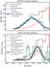 |
Fig. 14 Stacked GCLF of massive galaxies (top) and dwarf galaxies (bottom). The GCLF is derived for the final GC candidates in this work (selected based on their compactness, colour and ellipticity). The black histogram shows all GC candidates within 4 Re and 2 Re of a given host galaxy for massive and dwarf galaxies, respectively. The red histogram shows the magnitude distribution of background sources, and the blue histogram is the background-corrected histogram. The best fit Gaussian to the background-corrected histogram is shown as the black line. The histograms are completeness-corrected. The errorbars represent the Poisson uncertainties for the number of GC within the magnitude bin and take into account the Poisson uncertainties from the (subtracted) background. The displayed best Gaussian fit for the GCLF of dwarf galaxies is done including and excluding the GC excess between IE = 22.0 and 22.5., shown with grey and black curves, respectively. |
5.3.3 GC radial distribution
Here, we study this GC profile for the dwarf galaxies in our sample (30 dwarf galaxies). With the Euclid data and the GC sample presented here, one can inspect the stacked radial profile of GCs. For that purpose, we normalize the galactocentric distances of GCs to their host galaxy to the effective radius of the host (Re). Additionally, we only consider dwarf galaxies with a stellar mass of M* = 107 M⊙ and larger (14 galaxies) because they seem to have a few GC candidates. Stacking the GC radial distributions of these dwarf galaxies, we aim to enhance the low GC number statistics and reduce the statistical effect of contamination.
Figure 15 presents the GC radial profile of these dwarf galaxies. As is seen in this figure, GCs are distributed out to 3Re from their host dwarf galaxies. Beyond 3Re (2Re in the lower panel), the GC distribution reaches a plateau (i.e. has reached the ICGCs), consistent with being due to a uniform background. This is valid for the GCs brighter than IE = 23.0 (upper panel) and IE = 24.5 (lower panel). We fit a Sérsic profile to the stacked GC radial distribution to characterize this distribution. We quantify the radial profile of GCs by using the ratio between GC half-number radius and galaxies’ effective radius (RGC/Re). We estimate RGC/Re = 0.84 ± 0.27 and RGC/Re = 0.80 ± 0.22 for the GCs brighter than IE = 23.0 and IE = 24.5, respectively. The values of the Sérsic index are very uncertain and about 1.6 ± 1.9 and 0.5 ± 0.7 respectively. We note that the GC radial profile of dwarf galaxies presented here is produced excluding the NSCs. The GC radial profiles in Fig. 15 are based on 67 and 305 GC candidates within 5Re , for GCs brighter than IE = 23.0 and IE = 24.5, respectively. However, about half of these GCs are around three GC-rich dwarf galaxies in the sample (FDS16_DWARF257, FDS11_DWARF294, and FDS11_DWARF306). Therefore, the GC radial profile might be highly biased to these systems. However, we do not see any difference in GC profiles when we divide the three GC-rich systems and the rest of the dwarf galaxies.
These results do not support the common view of GC profile of dwarf galaxies with RGC/Re = 1.5 (van Dokkum et al. 2017; Lim et al. 2018). This ratio has been studied in a few more recent works using ground-based data of dwarf galaxies (Carlsten et al. 2022) and space-based data for GC-rich UDGs (Müller et al. 2021; Montes et al. 2021; Saifollahi et al. 2022; Janssens et al. 2022). Carlsten et al. (2022) studied dwarf galaxies in the local Volume, in galaxy groups and also in the Virgo cluster and found RGC/Re = 1.06 and RGC/Re = 1.25, respectively. Within uncertainties, the estimated RGC /Re in this work is consistent with Carlsten et al. (2022), but also indicates that GC distribution is even more compact. Carlsten et al. (2022) was based on optical ground-based imaging, and therefore the slightly higher values could arise from higher contamination in ground-based GC samples. However, our estimated RGC/Re is consistent with RGC/Re < 1 found for GC-rich UDGs using the HST. The fact that these objects are GC rich is the reason that the authors could estimate RGC/Re for these objects.
Overall, the estimated values of RGC/Re imply that the GCs of dwarf galaxies, regardless of being GC rich or GC poor, UDG or non-UDG, have a more compact radial distribution than the expectations for dwarf galaxies based on the previous works. This points to a diversity of GC properties of dwarf galaxies in their radial profile and potentially has implications for astrophysical processes that are involved in formation and evolution of various types of dwarf galaxies. Studying this diversity and understanding dwarf galaxies through their GCs is one of the main objectives of Legacy Science with the Euclid Wide Surveys.
Furthermore, based on the best-fit Sérsic function, the stacked radial distribution of GCs (Fig. 15) reaches the background level  and
and  for the GCs brighter than IE = 23.0 and IE = 24.5, respectively. On average, this corresponds to 0.04
  and 0.24
  GCs for each galaxy. Assuming an average Re = 1 kpc for the dwarf galaxies in the sample, these values convert to 0.04 kpc−2 and 0.24 kpc−2. In total, we estimate, 0.4 and 2.1 GCs within 3Re of each dwarf galaxy. The GC background originates from ICGCs and non-GCs. Therefore, the above-mentioned estimations provide an upper limit on the purity of the GC candidates and an upper limit on the contamination from non-GCs for their corresponding magnitude range.
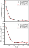 |
Fig. 15 Stacked radial distribution of the GC number density of dwarf galaxies (14 galaxies with stellar masses of M* > 107 M⊙) for GCs brighter than IE = 23 (upper panel) and GCs brighter than IE = 24.5 (lower panel). The GC radial distance from the centres of their host galaxies (x-axis) is normalised to the host galaxy’s effective radius (Re). The GC number density (y-axis) represents sum of GCs around all the 14 dwarf galaxies has the unit of |

6 Summary and conclusions
In this paper, we have presented the Euclid ERO data of a field in the Fornax cluster to investigate the potential of Euclid data for studying GCs, particularly around dwarf galaxies. We followed a step-by-step analysis to maximise the efficiency of source detection and the accuracy of the source photometry. We identified a catalogue of candidate GCs in the studied Fornax FoV using the Euclid data by modelling the PSF, performing source detection, and finally obtaining aperture photometry of all the detected sources. We then applied cuts in colour and compactness to select the most likely sources for our final GC candidate catalogue. We estimated the completeness of GC detection by injecting artificial GCs into the data.
Additionally, we assessed the performance of the GC detection using the spectroscopically known GCs as well as GC candidates of the ACSFCS. Overall, we recovered approximately 80% of GCs in IE and YE down to magnitude IE = 25.2. This is 1.7 mag fainter than the typical turnover magnitude of the GCLF at MV = −7.5. The completeness limit is driven by the NISP images, which in these early Euclid observations lack the ancillary data needed for more precise calibrations that became possible a few weeks later; the EWS data will be more complete.
The purity of the derived GC candidate catalogue is much harder to estimate because there is no easy way to know how many foreground and background contaminants remain after our colour and completeness cuts. Photometrically selected GC samples tend to have contamination, and only spectroscopic follow-up will show exactly what the purity of the sample is. Here, we assessed the purity of the bright GCs and showed that about 80% of the GC candidates for GCs brighter than IE = 21.5 are true GCs, based on the uiKs and gri colour-colour diagrams of GC candidates.
We used the final GC candidate catalogues to study the properties of the GCs surrounding dwarf galaxies in the Fornax cluster as well as the spatial distribution of the intracluster GCs. Our main findings are as follows:
We identified more than 5000 new GC candidates in the Fornax cluster and within the ERO-F FoV, brighter than IE = 25 (MV = −6). This magnitude corresponds to 1.5 mag fainter than the typical GCLF turnover magnitude (MV = −7.5) at the distance of the Fornax cluster. We showed that the ICGC sample is 70% complete at this magnitude. Furthermore, we discussed how the identified ICGCs follow a distribution similar to the ICL within the FoV;
Overall, dwarf galaxies in the Fornax cluster have NGC values consistent with the expectations for dwarf galaxies of their stellar mass. Three dwarf galaxies (UDG by definition) seem to have more GCs than the average and are thus GC rich. Dwarf galaxies less massive than M* = 107 M⊙ (Mr > −13.5) on average have no GCs, except in a few cases. In particular, we identified a few dwarf galaxies with a stellar mass less than M* = 106 M⊙ that have about one GC each;
The GCLF of dwarf galaxies does not seem to follow a Gaussian distribution. However, assuming that it is a Gaussian distribution, the GCLF has a turnover magnitude at about IE = 23.62 ± 0.42 (MV = −7.38 ± 0.42), which is consistent with values in the literature. However, the width of the GCLF of dwarf galaxies, σ = 1.00 ± 0.33, is larger than the expected value. This broadening of the GCLF arises from bright GCs with IE between 22 and 22.5 (MV = −9 and −8.5), and the majority of these GCs are associated with three of the dwarf galaxies in our sample. When excluding these bright GCs, we found a turnover magnitude of IE = 23.74 ± 0.14 (MV = −7.75 ± 0.14) and a narrower Gaussian distribution with σ = 0.52 ± 0.13, which is more consistent with the expectations for dwarf galaxies of the same stellar mass regime;
We found the ratio between the GC half-number radius and dwarf galaxy half-light radius: RGC/Re = 0.84 ± 0.27 and RGC/Re = 0.80 ± 0.22, for GCs brighter than IE = 23.0 and IE = 24.5, respectively. These numbers imply that in dwarf galaxies, GCs follow the same (or more compact) radial distribution as stars. These results do not support the current view of the GC profile of dwarf galaxies (with RGC/Re = 1.5) and indicate that the GC radial profile of dwarf galaxies is more compact. Furthermore, we discussed how this is similar to what has been observed for some of the UDGs. However, compared to those UDGs, the majority of dwarf galaxies studied here are poor in GCs (for their stellar mass), while the UDGs host two to three times more GCs.
We have shown in this paper that Euclid imaging is well suited to study dwarf galaxies in order to explore low GC-count systems and study the galaxy-GC-halo connection. With the upcoming EWS that will span 14 000 deg2 of the sky (Euclid Collaboration: Mellier et al. 2025), such studies will be possible for all the nearby galaxies and galaxy clusters besides the Fornax cluster.
Acknowledgements.
This work has made use of the Early Release Observations (ERO) data from the Euclid mission of the European Space Agency (ESA), 2024, https://doi.org/10.57780/esa-qmocze3. The Euclid Consortium acknowledges the European Space Agency and a number of agencies and institutes that have supported the development of Euclid, in particular the Agen- zia Spaziale Italiana, the Austrian Forschungsförderungsgesellschaft funded through BMK, the Belgian Science Policy, the Canadian Euclid Consortium, the Deutsches Zentrum für Luft- und Raumfahrt, the DTU Space and the Niels Bohr Institute in Denmark, the French Centre National d’Etudes Spatiales, the Fundação para a Ciência e a Tecnologia, the Hungarian Academy of Sciences, the Ministerio de Ciencia, Innovación y Universidades, the National Aeronautics and Space Administration, the National Astronomical Observatory of Japan, the Netherlandse Onderzoekschool Voor Astronomie, the Norwegian Space Agency, the Research Council of Finland, the Romanian Space Agency, the State Secretariat for Education, Research, and Innovation (SERI) at the Swiss Space Office (SSO), and the United Kingdom Space Agency. A complete and detailed list is available on the Euclid web site (http://www.euclid-ec.org). We thank the referee for their comments which helped to improve quality of this paper. TS, KV, AL acknowledge support from Agence Nationale de la Recherche, France, under project ANR-19-CE31-0022. MC acknowledges support from the project “INAF Exploration of Diffuse Galaxies with Euclid” (INAF-Large Grant 12-2022, P.I. Leslie K. Hunt). MAR acknowledges funding from the European Union’s Horizon 2020 research and innovation programme under the Marie Skłodowska-Curie grant agreement No 101066353 (project ELATE). This research has made use of the SIMBAD database (Wenger et al. 2000), operated at CDS, Strasbourg, France, the VizieR catalogue access tool (Ochsenbein et al. 2000), CDS, Strasbourg, France (DOI : 10.26093/cds/vizier), and the Aladin sky atlas (Bonnarel et al. 2000; Boch & Fernique 2014) developed at CDS, Strasbourg Observatory, France and SAOImageDS9 (Joye & Mandel 2003). This work has been done using the following software, packages and python libraries: Topcat (Taylor 2005); Numpy (van der Walt et al. 2011), Scipy (Virtanen et al. 2020), Astropy (Astropy Collaboration et al. 2018), Scikit-learn (Pedregosa et al. 2011).
Appendix A Fitting the GCLF using individual measurements.
We fit the stacked distribution of IE magnitudes of GC candidates located within 2 Re of dwarf galaxy centres, with two components: a Gaussian with mean magnitude µ and standard deviation σ, and an exponential that matches the distribution of IE of GC-candidates in background areas around the dwarfs down to IE = 25. The background count model is based on observations, and hence that component does not need to be multiplied by the completeness function c(m) (Fig. 3, top panel), but the Gaussian model of the dwarf component of the GCLF does. In practice, the completeness function remains very flat over the range of magnitudes that is actually used. Thus, the effect of c(m) is marginal. The resulting probability for any random GC to be detected within dm of magnitude m is written
![Mathematical equation: $p(m){\rm{d}}m = \underbrace {\left[ {c(m)\exp {{ - {{(m - \mu )}^2}} \over {2{\sigma ^2}}} + \beta \exp {{(m - 25)} \over {1.0}}} \right]}_{f(m;\mu ,\sigma ,\beta )}{\rm{d}}m/N(\mu ,\sigma ,\beta ),$](/articles/aa/full_html/2025/05/aa50784-24/aa50784-24-eq7.png) (A.1)
(A.1)
where N(µ, σ,β) is the integral of f (m; µ, σ,β) over the full range of magnitudes m that are being considered (in practice 20.5 ⩽ IE ⩽ 25), and
 (A.2)
(A.2)
The denominator of the argument of the second exponential in p(m) results from a fit, and varying it by ±5% has little effect on results. Similarly, the factors 1.0 in c(m) result from a fit (see Eq. 1). The photometric measurements have errors, and we represent the standard deviations s(m) with
![Mathematical equation: $s(m) = 0.01 + 0.07\exp [(m - 25)/1.2].$](/articles/aa/full_html/2025/05/aa50784-24/aa50784-24-eq9.png) (A.3)
(A.3)
That function implements a minimum uncertainty of 0.01 at magnitudes brighter than about 21.5 then a progressive increase so that the 1 σ uncertainties amount to 0.05 at IE = 24.2 and 0.1 at IE = 25.3. The stacked IE distribution in the magnitude range of interest contains N objects with individual magnitudes mi and individual uncertainties si. For a given (µ, σ,β), the probability of observing one object within si of mi is evaluated as
 (A.4)
(A.4)
and assuming independence between the data points, the likelihood of the data set is ℒ(µ, σ,β) = Πi Pi.
A maximum likelihood fit would assume flat priors for µ, σ and β. However, the GC-candidate counts on dwarf galaxies and around them provide prior information on β. In the background areas, there are 3718 GC candidates. In the on-dwarf areas, which cover 50 times less sky, we counted 112. Hence, the latter consists approximately of 74 contaminants and 38 true dwarf members. The ratio Rref is 1.95. We could allow for stochasticity roughly by assuming Poisson statistics:
 (A.5)
(A.5)
If we let G denote the integral of the first term of f (m) and β B the integral of the second term, the ratio β B/G should not be too far from Rref. This defines a first guess for β for any choice of µ and  . The prior on β is modelled with a Gaussian probability distribution,
![Mathematical equation: $p(\beta \mid \mu ,\sigma ) \propto \exp \left[ { - {{{{(\beta - \bar \beta )}^2}} \over {2\sigma _\beta ^2}}} \right],$](/articles/aa/full_html/2025/05/aa50784-24/aa50784-24-eq13.png) (A.6)
(A.6)
truncated to keep only β > 0 and normalised. We adopted σβ = 0.53 G/B. For our fits, we maximised a posterior probability that accounts for this prior.
The data and an example of the fit results are shown in Fig. A.1. The same figure for results after removing two-thirds of the GC candidates within IE = 22 and 22.5 is shown in Fig. A.2. In these figures, panel (a) presents the photometry of objects within 2 Re of the centres of 14 dwarf galaxies, with the errors just described. Panel (b) shows the same data after sorting and compares that distribution with the sorted magnitudes of all the sources in background rings around dwarf galaxies. Panel (c) shows the map of posterior probabilities obtained when, for each (µ, σ)-pair, the value of β that maximises the probability is retained. We checked that the range explored for β was sufficient, by verifying that it does not reach the extremes defined in the code for any (µ, σ)-pair in the region of interest. The white contour corresponds to an e-fold decrease in likelihood compared to the best fit, the black contour a 10-fold decrease. Finally, panel (d) shows the cumulative distributions of observed magnitudes together with the cumulative distribution of the best-fit model. The best fits are not very good fits: a KS-test returns a p-values around 0.26 and 0.30, respectively (We note that the KS-test does not take into account photometric errors). These p-values mean that deviations from the modelled cumulative distribution as large as observed would result from random realisation more than one time out of four; in other words, the Gaussian model for the dwarf GCLF cannot be safely excluded.
The inferred magnitude distributions for the background objects and the dwarf GCs are shown separately in Fig. A.3, for the same fitting parameters as in Fig. A.2 (that is after excluding two-thirds of the bright GCs within IE = 22.0 and 22.5). Although the peak of the dwarf GCLF model occurs at 23.7, the contrast with respect to background sources is highest at about 23.5. We recall that the sample of GC candidates examined here results from selection criteria that are more permissive than, for instance, the selection used to investigate the spatial distribution of GCs within the full FoV (see last paragraph of Sect. 4); the modelling done here handles the contamination by explicitly including that component.
 |
Fig. A.1 Data set of individual IE magnitudes of GC candidates and fits to the GCLF. (a): photometry of objects within 2 Re of the centres of 14 dwarf galaxies. (b): same data after sorting (green), compared with the sorted magnitudes of all the sources in background rings around dwarf galaxies (red). (c): map of posterior probabilities obtained when, for each (µ, σ)-pair, the value of β that maximises the posterior probability is retained. The white and black contours correspond, respectively, to an e-fold and a 10-fold decrease in probability compared to the best fit. (d): cumulative distributions of observed magnitudes together with the cumulative distribution of the best-fit model (black line). |
Appendix B Colours and colour transformations for old stellar populations
For convenience, Fig. B.1 displays the colour-colour diagrams relevant to the transformations of GC magnitudes from external catalogues to the Euclid system, and to the intrinsic colours of GCs in Euclid passbands. Because the GCs around early-type galaxies are typically old and well represented with a singleage population, we restrict the models to so-called simple stellar populations (SSP) with ages older than 7 Gyr (and younger than 15 Gyr). The V band in Panel (a) is from Bessell (1990), and that panel was used to convert V -band GCLF-properties from Rejkuba (2012) to the Euclid system. The g band in Panel (b) of Fig. B.1 refers to the OmegaCAM instrument on VST (Vista Survey Telescope, European Southern Observatory), as used in the Fornax Deep Survey. The F850LP passband in Panel (c) is from the Advanced Camera for Surveys onboard the Hubble Space Telescope used in the ACS Fornax Cluster Survey; F475W, also used in that survey, is not shown, because its synthetic photometry is identical to that of the VST g band to better than 4%. Panel (d) displays JE − HE vs IE − YE, for comparison with Figs. 5 and 6 used to implement a colour-selection for GC candidates. The models used in all panels, and their main ingredients, are listed below.
Padova PC (Bressan et al. 2012; Marigo et al. 2017): isochrones as available in the default configuration of the Padova distribution8 in early 2024, i.e. with Parsec 1.2 (Tang et al. 2014; Chen et al. 2015) with the TP-AGB extension of the Colibri code (Pastorelli et al. 2019, 2020).
Pégase (Fioc & Rocca-Volmerange 1997, hereafter FRV97; Le Borgne et al. 2004): stellar evolution tracks mainly from the Padova group (published 1993–1996), but extended through the thermally pulsing asymptotic giant branch (AGB) and to the post-AGB as described in FRV97; isochrones computed on-the-fly; and BaSeL spectral library (Lejeune et al. 1997, 1998).
XSL iSSP (Verro et al. 2022a) : Parsec-Colibri isochrones as in Padova PC above, but with colours based on the empirical spectra from the X-shooter Spectral Library (Verro et al. 2022b).
BC03 (Bruzual & Charlot 2003, 2016 version9): Padova isochrones (1994+); and BaSeL3.1 spectral library (Westera et al. 2002).
SL Synthe: Models computed using BaSTI isochrones (Hidalgo et al. 2018; Pietrinferni et al. 2021) and synthetic spectra produced with ATLAS or MARCS stellar atmospheres
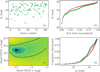 |
Fig. A.2 Similar to Fig. A.1 but after removing about two-thirds of the GC candidates (seven) between IE = 22 and 22.5. |
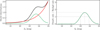 |
Fig. A.3 Derived model for the luminosity distribution of GC candidates towards dwarf galaxies. Left panel: Inferred magnitude distributions for the fit carried out within the range 20.5 < IE < 25, excluding two-thirds of the bright GCs (as in Fig. A.2). The distributions for all GC candidates for the background GCs (exponential) and for the dwarf-galaxy GCs (Gaussian) are shown in black, red, and green, respectively. Right panel: Ratio of the dwarf GCLF to the background GCLF in the model, with ratios of one and 1.6 highlighted. |
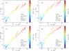 |
Fig. B.1 Colour-colour relations based on synthetic photometry carried out on the spectra produced for old SSPs with various population synthesis codes (see text for details). (a) Colour transformation from the generic V band of Bessell (1990) to the Euclid system, used for converting the GCLF-properties of Rejkuba (2012). (b) Colour transformation from the g passband of the OmegaCAM instrument on VST (European Southern Observatory), used for comparisons with the FDS survey. (c) Colour transformation from the F850LP passband of the Advanced Camera for Surveys on HST, as used in the ACSFCS survey of the Fornax cluster; F475W photometry differs from the g-band photometry of panel (a) by less than 4% and is not shown. (d) Colours of old single stellar populations in a Euclid colour-colour plane. All passband transmissions used include the filter, the instrument, and the detector. |
(Kurucz 1970; Gustafsson et al. 2008) and the SYNTHE and Turbospectrum spectral synthesis codes (Kurucz & Avrett 1981; Kurucz 2005; Alvarez & Plez 1998). See Larsen et al. (2022) for details.
Appendix C Cutouts of dwarf galaxies and their GC candidates
In figures C.1 and C.2, Euclid VIS image cutouts of 30 dwarf galaxies and their GC candidates are presented.
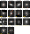 |
Fig. C.1 Euclid VIS image cutouts centred on 14 Fornax cluster dwarf galaxies with stellar masses of M* > 107 M⊙ (studied in this work). The order is from the highest stellar mass (top left) to the lowest stellar mass (bottom right). |
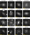 |
Fig. C.2 Euclid VIS image cutouts centred on 16 Fornax cluster dwarf galaxies with stellar mass M* < 107 M⊙ (studied in this work). The order is from the highest stellar mass (top left) to the lowest stellar mass (bottom right). |
References
- Abbott, T. M. C., Adamów, M., Aguena, M., et al. 2021, ApJS, 255, 20 [NASA ADS] [CrossRef] [Google Scholar]
- Alamo-Martínez, K. A., Blakeslee, J. P., Jee, M. J., et al. 2013, ApJ, 775, 20 [CrossRef] [Google Scholar]
- Alvarez, R., & Plez, B. 1998, A&A, 330, 1109 [NASA ADS] [Google Scholar]
- Astropy Collaboration (Price-Whelan, A. M., et al.) 2018, AJ, 156, 123 [Google Scholar]
- Bassino, L. P., Cellone, S. A., Forte, J. C., & Dirsch, B. 2003, A&A, 399, 489 [NASA ADS] [CrossRef] [EDP Sciences] [Google Scholar]
- Bassino, L. P., Richtler, T., & Dirsch, B. 2006, MNRAS, 367, 156 [NASA ADS] [CrossRef] [Google Scholar]
- Bastian, N., Pfeffer, J., Kruijssen, J. M. D., et al. 2020, MNRAS, 498, 1050 [Google Scholar]
- Baumgardt, H., Hilker, M., Sollima, A., & Bellini, A. 2019, MNRAS, 482, 5138 [Google Scholar]
- Beasley, M. A., Trujillo, I., Leaman, R., & Montes, M. 2018, Nature, 555, 483 [NASA ADS] [CrossRef] [Google Scholar]
- Beasley, M. A., Leaman, R., Gallart, C., et al. 2019, MNRAS, 487, 1986 [Google Scholar]
- Bergond, G., Athanassoula, E., Leon, S., et al. 2007, A&A, 464, L21 [NASA ADS] [CrossRef] [EDP Sciences] [Google Scholar]
- Bertin, E., & Arnouts, S. 1996, A&AS, 117, 393 [NASA ADS] [CrossRef] [EDP Sciences] [Google Scholar]
- Bertin, E., Mellier, Y., Radovich, M., et al. 2002, The TERAPIX Pipeline, Astronomical Society of the Pacific Conference Series, 281, 228 [Google Scholar]
- Bessell, M. S. 1990, PASP, 102, 1181 [NASA ADS] [CrossRef] [Google Scholar]
- Blakeslee, J. P., Jordán, A., Mei, S., et al. 2009, ApJ, 694, 556 [Google Scholar]
- Boch, T., & Fernique, P. 2014, in Astronomical Data Analysis Software and Systems XXIII, eds. N. Manset, & P. Forshay, Astronomical Society of the Pacific Conference Series, 485, 277 [Google Scholar]
- Bonnarel, F., Fernique, P., Bienaymé, O., et al. 2000, A&AS, 143, 33 [NASA ADS] [CrossRef] [EDP Sciences] [Google Scholar]
- Bressan, A., Marigo, P., Girardi, L., et al. 2012, MNRAS, 427, 127 [NASA ADS] [CrossRef] [Google Scholar]
- Bruzual, G., & Charlot, S. 2003, MNRAS, 344, 1000 [NASA ADS] [CrossRef] [Google Scholar]
- Burkert, A., & Forbes, D. A. 2020, AJ, 159, 56 [Google Scholar]
- Buzzo, M. L., Forbes, D. A., Jarrett, T. H., et al. 2024, MNRAS, 529, 3210 [NASA ADS] [CrossRef] [Google Scholar]
- Cantiello, M., Venhola, A., Grado, A., et al. 2020, A&A, 639, A136 [NASA ADS] [CrossRef] [EDP Sciences] [Google Scholar]
- Carleton, T., Guo, Y., Munshi, F., Tremmel, M., & Wright, A. 2021, MNRAS, 502, 398 [NASA ADS] [CrossRef] [Google Scholar]
- Carlsten, S. G., Greene, J. E., Beaton, R. L., & Greco, J. P. 2022, ApJ, 927, 44 [NASA ADS] [CrossRef] [Google Scholar]
- Chaturvedi, A., Hilker, M., Cantiello, M., et al. 2022, A&A, 657, A93 [NASA ADS] [CrossRef] [EDP Sciences] [Google Scholar]
- Chen, Y., Bressan, A., Girardi, L., et al. 2015, MNRAS, 452, 1068 [Google Scholar]
- Chen, Z., Stark, D. P., Endsley, R., et al. 2023, MNRAS, 518, 5607 [Google Scholar]
- Cole, A. A., Weisz, D. R., Skillman, E. D., et al. 2017, ApJ, 837, 54 [NASA ADS] [CrossRef] [Google Scholar]
- Creasey, P., Sales, L. V., Peng, E. W., & Sameie, O. 2019, MNRAS, 482, 219 [Google Scholar]
- Cuillandre, J.-C., Bertin, E., Bolzonella, M., et al. 2025, A&A, 697, A6 (Euclid on Sky SI) [Google Scholar]
- D’Abrusco, R., Cantiello, M., Paolillo, M., et al. 2016, ApJ, 819, L31 [CrossRef] [Google Scholar]
- Danieli, S., van Dokkum, P., Trujillo-Gomez, S., et al. 2022, ApJ, 927, L28 [NASA ADS] [CrossRef] [Google Scholar]
- de Boer, T. J. L., & Fraser, M. 2016, A&A, 590, A35 [NASA ADS] [CrossRef] [EDP Sciences] [Google Scholar]
- De Bórtoli, B. J., Caso, J. P., Ennis, A. I., & Bassino, L. P. 2022, MNRAS, 510, 5725 [CrossRef] [Google Scholar]
- Diego, J. M., Pascale, M., Frye, B., et al. 2023, A&A, 679, A159 [NASA ADS] [CrossRef] [EDP Sciences] [Google Scholar]
- Dold, D., & Fahrion, K. 2022, A&A, 663, A81 [NASA ADS] [CrossRef] [EDP Sciences] [Google Scholar]
- Drinkwater, M. J., Phillipps, S., Jones, J. B., et al. 2000, A&A, 355, 900 [NASA ADS] [Google Scholar]
- Drinkwater, M. J., Gregg, M. D., & Colless, M. 2001, ApJ, 548, L139 [Google Scholar]
- Durrell, P. R., Harris, W. E., Geisler, D., & Pudritz, R. E. 1996, AJ, 112, 972 [Google Scholar]
- Eigenthaler, P., Puzia, T. H., Taylor, M. A., et al. 2018, ApJ, 855, 142 [Google Scholar]
- El-Badry, K., Quataert, E., Weisz, D. R., Choksi, N., & Boylan-Kolchin, M. 2019, MNRAS, 482, 4528 [Google Scholar]
- Euclid Collaboration (Scaramella, R., et al.) 2022, A&A, 662, A112 [NASA ADS] [CrossRef] [EDP Sciences] [Google Scholar]
- Euclid Collaboration (Schirmer, M., et al.) 2022, A&A, 662, A92 [NASA ADS] [CrossRef] [EDP Sciences] [Google Scholar]
- Euclid Collaboration (Cropper, M., et al.) 2025, A&A, 697, A2 (Euclid on Sky SI) [Google Scholar]
- Euclid Collaboration (Jahnke, K., et al.) 2025, A&A, 697, A3 (Euclid on Sky SI) [Google Scholar]
- Euclid Collaboration (Mellier, Y., et al.) 2025, A&A, 697, A1 (Euclid on Sky SI) [Google Scholar]
- Euclid Collaboration (Voggel, K., et al.) 2025, A&A, 693, A251 [Google Scholar]
- Euclid Early Release Observations 2024, https://doi.org/10.57780/esa-qmocze3 [Google Scholar]
- Fahrion, K., Lyubenova, M., Hilker, M., et al. 2020, A&A, 637, A26 [NASA ADS] [CrossRef] [EDP Sciences] [Google Scholar]
- Fahrion, K., Leaman, R., Lyubenova, M., & van de Ven, G. 2022, A&A, 658, A172 [NASA ADS] [CrossRef] [EDP Sciences] [Google Scholar]
- Faisst, A. L., Chary, R. R., Brammer, G., & Toft, S. 2022, ApJ, 941, L11 [NASA ADS] [CrossRef] [Google Scholar]
- Federle, S., Gómez, M., Mieske, S., et al. 2024, A&A, 689, A342 [NASA ADS] [CrossRef] [EDP Sciences] [Google Scholar]
- Ferré-Mateu, A., Gannon, J. S., Forbes, D. A., et al. 2023, MNRAS, 526, 4735 [CrossRef] [Google Scholar]
- Fioc, M., & Rocca-Volmerange, B. 1997, A&A, 326, 950 [NASA ADS] [Google Scholar]
- Firth, P., Drinkwater, M. J., Evstigneeva, E. A., et al. 2007, MNRAS, 382, 1342 [NASA ADS] [CrossRef] [Google Scholar]
- Firth, P., Drinkwater, M. J., & Karick, A. M. 2008, MNRAS, 389, 1539 [NASA ADS] [CrossRef] [Google Scholar]
- Fleming, D. E. B., Harris, W. E., Pritchet, C. J., & Hanes, D. A. 1995, AJ, 109, 1044 [Google Scholar]
- Forbes, D. A., & Gannon, J. 2024, MNRAS, 528, 608 [NASA ADS] [CrossRef] [Google Scholar]
- Forbes, D. A., Read, J. I., Gieles, M., & Collins, M. L. M. 2018, MNRAS, 481, 5592 [NASA ADS] [CrossRef] [Google Scholar]
- Gannon, J. S., Ferré-Mateu, A., Forbes, D. A., et al. 2024, MNRAS, 531, 1856 [NASA ADS] [CrossRef] [Google Scholar]
- Georgiev, I. Y., Hilker, M., Puzia, T. H., Goudfrooij, P., & Baumgardt, H. 2009, MNRAS, 396, 1075 [NASA ADS] [CrossRef] [Google Scholar]
- Georgiev, I. Y., Puzia, T. H., Goudfrooij, P., & Hilker, M. 2010, MNRAS, 406, 1967 [NASA ADS] [Google Scholar]
- Gieles, M., & Gnedin, O. Y. 2023, MNRAS, 522, 5340 [NASA ADS] [CrossRef] [Google Scholar]
- Gregg, M. D., Drinkwater, M. J., Evstigneeva, E., et al. 2009, AJ, 137, 498 [NASA ADS] [CrossRef] [Google Scholar]
- Gustafsson, B., Edvardsson, B., Eriksson, K., et al. 2008, A&A, 486, 951 [NASA ADS] [CrossRef] [EDP Sciences] [Google Scholar]
- Gvozdenko, A., Larsen, S. S., Beasley, M. A., & Brodie, J. 2022, A&A, 666, A159 [NASA ADS] [CrossRef] [EDP Sciences] [Google Scholar]
- Harris, W. E. 1991, ARA&A, 29, 543 [Google Scholar]
- Harris, W. E. 1996, AJ, 112, 1487 [Google Scholar]
- Harris, W. E., & Reina-Campos, M. 2023, MNRAS, 526, 2696 [NASA ADS] [CrossRef] [Google Scholar]
- Harris, W. E., Harris, G. L. H., & Alessi, M. 2013, ApJ, 772, 82 [Google Scholar]
- Harris, W. E., Blakeslee, J. P., & Harris, G. L. H. 2017, ApJ, 836, 67 [Google Scholar]
- Harris, W. E., Brown, R. A., Durrell, P. R., et al. 2020, ApJ, 890, 105 [NASA ADS] [CrossRef] [Google Scholar]
- Hidalgo, S. L., Pietrinferni, A., Cassisi, S., et al. 2018, ApJ, 856, 125 [Google Scholar]
- Hilker, M., Infante, L., Vieira, G., Kissler-Patig, M., & Richtler, T. 1999, A&AS, 134, 75 [NASA ADS] [CrossRef] [EDP Sciences] [Google Scholar]
- Hilker, M., Baumgardt, H., Sollima, A., & Bellini, A. 2020, in Star Clusters: From the Milky Way to the Early Universe, 351, eds. A. Bragaglia, M. Davies, A. Sills, & E. Vesperini, 451 [NASA ADS] [Google Scholar]
- Horta, D., Hughes, M. E., Pfeffer, J. L., et al. 2021, MNRAS, 500, 4768 [Google Scholar]
- Hudson, M. J., & Robison, B. 2018, MNRAS, 477, 3869 [NASA ADS] [CrossRef] [Google Scholar]
- Hunt, L., Annibali, F., Cuillandre, J.-C., et al. 2025, A&A, 697, A9 (Euclid on Sky SI) [NASA ADS] [CrossRef] [EDP Sciences] [Google Scholar]
- Iodice, E., Capaccioli, M., Grado, A., et al. 2016, ApJ, 820, 42 [Google Scholar]
- Iodice, E., Spavone, M., Capaccioli, M., et al. 2017, ApJ, 839, 21 [Google Scholar]
- Janssens, S. R., Romanowsky, A. J., Abraham, R., et al. 2022, MNRAS, 517, 858 [NASA ADS] [CrossRef] [Google Scholar]
- Johnston, E. J., Puzia, T. H., D’Ago, G., et al. 2020, MNRAS, 495, 2247 [Google Scholar]
- Jordán, A., McLaughlin, D. E., Côté, P., et al. 2007, ApJS, 171, 101 [CrossRef] [Google Scholar]
- Jordán, A., Peng, E. W., Blakeslee, J. P., et al. 2015, ApJS, 221, 13 [Google Scholar]
- Joye, W. A., & Mandel, E. 2003, in Astronomical Data Analysis Software and Systems XII, eds. H. E. Payne, R. I. Jedrzejewski, & R. N. Hook, Astronomical Society of the Pacific Conference Series, 295, 489 [NASA ADS] [Google Scholar]
- King, I. 1962, AJ, 67, 471 [Google Scholar]
- King, I. R. 1966, AJ, 71, 276 [NASA ADS] [CrossRef] [Google Scholar]
- Kissler-Patig, M. 1997, A&A, 319, 83 [NASA ADS] [Google Scholar]
- Kluge, M., Hatch, N., Montes, M., et al. 2025, A&A, 697, A13 (Euclid on Sky SI) [NASA ADS] [CrossRef] [EDP Sciences] [Google Scholar]
- Kruijssen, J. M. D., Pfeffer, J. L., Crain, R. A., & Bastian, N. 2019, MNRAS, 486, 3134 [NASA ADS] [CrossRef] [Google Scholar]
- Kurucz, R. L. 1970, SAO Special Report, 309 [Google Scholar]
- Kurucz, R. L. 2005, Mem. Soc. Astron. Ital. Suppl., 8, 14 [Google Scholar]
- Kurucz, R. L., & Avrett, E. H. 1981, SAO Special Report, 391 [Google Scholar]
- La Marca, A., Iodice, E., Cantiello, M., et al. 2022, A&A, 665, A105 [NASA ADS] [CrossRef] [EDP Sciences] [Google Scholar]
- Larsen, S. S., Eitner, P., Magg, E., et al. 2022, A&A, 660, A88 [NASA ADS] [CrossRef] [EDP Sciences] [Google Scholar]
- Le Borgne, D., Rocca-Volmerange, B., Prugniel, P., et al. 2004, A&A, 425, 881 [CrossRef] [EDP Sciences] [Google Scholar]
- Lee, M. G., Bae, J. H., & Jang, I. S. 2022, ApJ, 940, L19 [NASA ADS] [CrossRef] [Google Scholar]
- Lejeune, T., Cuisinier, F., & Buser, R. 1997, A&AS, 125, 229 [NASA ADS] [CrossRef] [EDP Sciences] [Google Scholar]
- Lejeune, T., Cuisinier, F., & Buser, R. 1998, A&AS, 130, 65 [NASA ADS] [CrossRef] [EDP Sciences] [Google Scholar]
- Lim, S., & Lee, M. G. 2015, ApJ, 804, 123 [NASA ADS] [CrossRef] [Google Scholar]
- Lim, S., Peng, E. W., Côté, P., et al. 2018, ApJ, 862, 82 [Google Scholar]
- Liu, Y., Peng, E. W., Jordán, A., et al. 2019, ApJ, 875, 156 [NASA ADS] [CrossRef] [Google Scholar]
- Liu, C., Côté, P., Peng, E. W., et al. 2020, ApJS, 250, 17 [NASA ADS] [CrossRef] [Google Scholar]
- Lotz, J. M., Miller, B. W., & Ferguson, H. C. 2004, ApJ, 613, 262 [NASA ADS] [CrossRef] [Google Scholar]
- Maddox, N., Serra, P., Venhola, A., et al. 2019, MNRAS, 490, 1666 [Google Scholar]
- Marigo, P., Girardi, L., Bressan, A., et al. 2017, ApJ, 835, 77 [Google Scholar]
- Marleau, F. R., Habas, R., Poulain, M., et al. 2021, A&A, 654, A105 [NASA ADS] [CrossRef] [EDP Sciences] [Google Scholar]
- Marleau, F., Cuillandre, J.-C., Cantiello, M., et al. 2025, A&A, 697, A12 (Euclid on Sky SI) [NASA ADS] [CrossRef] [EDP Sciences] [Google Scholar]
- Martis, N. S., Sarrouh, G. T. E., Willott, C. J., et al. 2024, ApJ, 975, 76 [NASA ADS] [CrossRef] [Google Scholar]
- Massari, D., Koppelman, H. H., & Helmi, A. 2019, A&A, 630, L4 [NASA ADS] [CrossRef] [EDP Sciences] [Google Scholar]
- Massari, D., Dalessandro, E., Erkal, D., et al. 2025, A&A, 697, A8 (Euclid on Sky SI) [Google Scholar]
- Masters, K. L., Jordán, A., Côté, P., et al. 2010, ApJ, 715, 1419 [NASA ADS] [CrossRef] [Google Scholar]
- Mieske, S., Hilker, M., & Infante, L. 2004, A&A, 418, 445 [NASA ADS] [CrossRef] [EDP Sciences] [Google Scholar]
- Miller, B. W., & Lotz, J. M. 2007, ApJ, 670, 1074 [NASA ADS] [CrossRef] [Google Scholar]
- Miller, B. W., Lotz, J. M., Ferguson, H. C., Stiavelli, M., & Whitmore, B. C. 1998, ApJ, 508, L133 [Google Scholar]
- Misgeld, I., & Hilker, M. 2011, MNRAS, 414, 3699 [Google Scholar]
- Mohammadi, M., Mutatiina, J., Saifollahi, T., & Bunte, K. 2022, Astron. Comput., 39, 100555 [NASA ADS] [CrossRef] [Google Scholar]
- Montes, M., Trujillo, I., Infante-Sainz, R., Monelli, M., & Borlaff, A. S. 2021, ApJ, 919, 56 [NASA ADS] [CrossRef] [Google Scholar]
- Muñoz, R. P., Puzia, T. H., Lançon, A., et al. 2014, ApJS, 210, 4 [Google Scholar]
- Müller, O., Durrell, P. R., Marleau, F. R., et al. 2021, ApJ, 923, 9 [CrossRef] [Google Scholar]
- Ochsenbein, F., Bauer, P., & Marcout, J. 2000, A&AS, 143, 23 [NASA ADS] [CrossRef] [EDP Sciences] [Google Scholar]
- Ordenes-Briceño, Y., Puzia, T. H., Eigenthaler, P., et al. 2018, ApJ, 860, 4 [CrossRef] [Google Scholar]
- Pastorelli, G., Marigo, P., Girardi, L., et al. 2019, MNRAS, 485, 5666 [Google Scholar]
- Pastorelli, G., Marigo, P., Girardi, L., et al. 2020, MNRAS, 498, 3283 [Google Scholar]
- Pedregosa, F., Varoquaux, G., Gramfort, A., et al. 2011, J. Mach. Learn. Res., 12, 2825 [Google Scholar]
- Peletier, R., Iodice, E., Venhola, A., et al. 2020, arXiv e-prints [arXiv:2008.12633] [Google Scholar]
- Peng, E. W., Jordán, A., Côté, P., et al. 2008, ApJ, 681, 197 [NASA ADS] [CrossRef] [Google Scholar]
- Peng, E. W., Ferguson, H. C., Goudfrooij, P., et al. 2011, ApJ, 730, 23 [Google Scholar]
- Pfeffer, J., Kruijssen, J. M. D., Crain, R. A., & Bastian, N. 2018, MNRAS, 475, 4309 [Google Scholar]
- Pietrinferni, A., Hidalgo, S., Cassisi, S., et al. 2021, ApJ, 908, 102 [NASA ADS] [CrossRef] [Google Scholar]
- Pota, V., Napolitano, N. R., Hilker, M., et al. 2018, MNRAS, 481, 1744 [Google Scholar]
- Powalka, M., Lançon, A., Puzia, T. H., et al. 2016, ApJS, 227, 12 [Google Scholar]
- Prole, D. J., Davies, J. I., Keenan, O. C., & Davies, L. J. M. 2018, MNRAS, 478, 667 [NASA ADS] [CrossRef] [Google Scholar]
- Prole, D. J., Hilker, M., van der Burg, R. F. J., et al. 2019, MNRAS, 484, 4865 [Google Scholar]
- Reina-Campos, M., Hughes, M. E., Kruijssen, J. M. D., et al. 2020, MNRAS, 493, 3422 [Google Scholar]
- Rejkuba, M. 2012, Ap&SS, 341, 195 [Google Scholar]
- Román, J., Castilla, A., & Pascual-Granado, J. 2021, A&A, 656, A44 [NASA ADS] [CrossRef] [EDP Sciences] [Google Scholar]
- Román, J., Sánchez-Alarcón, P. M., Knapen, J. H., & Peletier, R. 2023, A&A, 671, L7 [NASA ADS] [CrossRef] [EDP Sciences] [Google Scholar]
- Romanowsky, A. J., Larsen, S. S., Villaume, A., et al. 2023, MNRAS, 518, 3164 [Google Scholar]
- Saifollahi, T., Janz, J., Peletier, R. F., et al. 2021a, MNRAS, 504, 3580 [NASA ADS] [CrossRef] [Google Scholar]
- Saifollahi, T., Trujillo, I., Beasley, M. A., Peletier, R. F., & Knapen, J. H. 2021b, MNRAS, 502, 5921 [NASA ADS] [CrossRef] [Google Scholar]
- Saifollahi, T., Zaritsky, D., Trujillo, I., et al. 2022, MNRAS, 511, 4633 [NASA ADS] [CrossRef] [Google Scholar]
- Sánchez-Janssen, R., Côté, P., Ferrarese, L., et al. 2019, ApJ, 878, 18 [CrossRef] [Google Scholar]
- Schuberth, Y., Richtler, T., Hilker, M., et al. 2010, A&A, 513, A52 [NASA ADS] [CrossRef] [EDP Sciences] [Google Scholar]
- Shen, Z., van Dokkum, P., & Danieli, S. 2021, ApJ, 909, 179 [CrossRef] [Google Scholar]
- Spavone, M., Iodice, E., van de Ven, G., et al. 2020, A&A, 639, A14 [NASA ADS] [CrossRef] [EDP Sciences] [Google Scholar]
- Spitler, L. R., & Forbes, D. A. 2009, MNRAS, 392, L1 [Google Scholar]
- Tang, J., Bressan, A., Rosenfield, P., et al. 2014, MNRAS, 445, 4287 [NASA ADS] [CrossRef] [Google Scholar]
- Taylor, M. B. 2005, in Astronomical Data Analysis Software and Systems XIV, eds. P. Shopbell, M. Britton, & R. Ebert, Astronomical Society of the Pacific Conference Series, 347, 29 [NASA ADS] [Google Scholar]
- Taylor, E. N., Hopkins, A. M., Baldry, I. K., et al. 2011, MNRAS, 418, 1587 [Google Scholar]
- Turner, M. L., Côté, P., Ferrarese, L., et al. 2012, ApJS, 203, 5 [NASA ADS] [CrossRef] [Google Scholar]
- Valenzuela, L. M., Moster, B. P., Remus, R.-S., O’Leary, J. A., & Burkert, A. 2021, MNRAS, 505, 5815 [NASA ADS] [CrossRef] [Google Scholar]
- van der Walt, S., Colbert, S. C., & Varoquaux, G. 2011, Comput. Sci. Eng., 13, 22 [Google Scholar]
- van Dokkum, P. G., Abraham, R., Merritt, A., et al. 2015, ApJ, 798, L45 [NASA ADS] [CrossRef] [Google Scholar]
- van Dokkum, P., Abraham, R., Romanowsky, A. J., et al. 2017, ApJ, 844, L11 [NASA ADS] [CrossRef] [Google Scholar]
- van Dokkum, P., Cohen, Y., Danieli, S., et al. 2018a, ApJ, 856, L30 [NASA ADS] [CrossRef] [Google Scholar]
- van Dokkum, P., Danieli, S., Cohen, Y., et al. 2018b, Nature, 555, 629 [Google Scholar]
- van Dokkum, P., Danieli, S., Abraham, R., Conroy, C., & Romanowsky, A. J. 2019, ApJ, 874, L5 [Google Scholar]
- Vanzella, E., Calura, F., Meneghetti, M., et al. 2017, MNRAS, 467, 4304 [Google Scholar]
- Veljanoski, J., Ferguson, A. M. N., Huxor, A. P., et al. 2013, MNRAS, 435, 3654 [NASA ADS] [CrossRef] [Google Scholar]
- Veljanoski, J., Ferguson, A. M. N., Mackey, A. D., et al. 2015, MNRAS, 452, 320 [NASA ADS] [CrossRef] [Google Scholar]
- Venhola, A., Peletier, R., Laurikainen, E., et al. 2018, A&A, 620, A165 [NASA ADS] [CrossRef] [EDP Sciences] [Google Scholar]
- Venhola, A., Peletier, R. F., Salo, H., et al. 2022, A&A, 662, A43 [NASA ADS] [CrossRef] [EDP Sciences] [Google Scholar]
- Verro, K., Trager, S. C., Peletier, R. F., et al. 2022a, A&A, 661, A50 [NASA ADS] [CrossRef] [EDP Sciences] [Google Scholar]
- Verro, K., Trager, S. C., Peletier, R. F., et al. 2022b, A&A, 660, A34 [NASA ADS] [CrossRef] [EDP Sciences] [Google Scholar]
- Villegas, D., Jordán, A., Peng, E. W., et al. 2010, ApJ, 717, 603 [Google Scholar]
- Virtanen, P., Gommers, R., Oliphant, T. E., et al. 2020, Nature Methods, 17, 261 [CrossRef] [Google Scholar]
- Wenger, M., Ochsenbein, F., Egret, D., et al. 2000, A&AS, 143, 9 [NASA ADS] [CrossRef] [EDP Sciences] [Google Scholar]
- Westera, P., Lejeune, T., Buser, R., Cuisinier, F., & Bruzual, G. 2002, A&A, 381, 524 [NASA ADS] [CrossRef] [EDP Sciences] [Google Scholar]
- Wittmann, C., Lisker, T., Pasquali, A., Hilker, M., & Grebel, E. K. 2016, MNRAS, 459, 4450 [NASA ADS] [CrossRef] [Google Scholar]
Expressed in the Vega magnitude system here.
Note that FCC161 (NGC1379) is among the galaxies in the ACSFCS survey; however, its HST data are corrupted and have not been used in ACSFCS publications.
Compilation of these catalogues are provided by Wittmann et al. (2016) and Maddox et al. (2019), with ground−based optical and nearinfrared photometry in Saifollahi et al. (2021a).
The source code for the analysis described in this paper is available at https://github.com/teymursaif/GCEx
With this definition, which agrees with common practice, large values of C2-4 and C4-8 imply less concentrated (more extended) profiles, which in the literature has led some authors to rename the same quantities ‘inverse concentration indices’.
The diffuse light within the ERO-F data is a mixture of ICL and the extended stellar halo of galaxies. Here for simplicity, we only refer to it as the ICL.
Gannon et al. (2024) provides spectroscopic properties as well as GC numbers of UDGs and it is compilation of several works.
All Tables
Properties of the ten most massive galaxies located within the footprint of the Euclid ERO-F images.
SExtractor parameters that were used for making detection frames and source extraction.
All Figures
|
Fig. 1 Field of view of the Euclid observations of the ERO Fornax cluster (ERO-F) presented in this paper. North is up and east is to the left. The stack of four VIS images is shown in translucent grey above a colour image from the Fornax Deep Survey (FDS), which shows the brightest cluster galaxy NGC 1399 just off the Euclid pointing in the south-east. The ERO-F field includes ten massive galaxies previously targeted by the ACSFCS (small inset images) around which about 900 GC candidates were identified by that survey (yellow dots: GC probability pGC > 0.95; Jordán et al. 2015). The galaxy FCC161 (NGC1379) is among the galaxies in the ACSFCS survey; however, its final HST data are corrupted. Therefore, no ACSFCS GC catalogue for this galaxy has been published. Additionally, the Euclid FoV overlaps with the position of about 30 dwarf galaxies (large green dots; Venhola et al. 2018, 2022) and about 602 spectroscopically confirmed GCs (red dots; references in the text). |
| In the text | |
|
Fig. 2 Euclid IE data (two-image stacked frame) versus the Dark Energy Survey (Abbott et al. 2021) in the r band for a cutout around dwarf galaxy FCC188 (FDS11_DWARF155). The galaxy is surrounded by several small point-like sources, some of which are the GCs of the galaxy. Given the high-resolution images of Euclid in IE , we are were to resolve the majority of GCs around similar objects and distinguish them from foreground stars. These images have a total exposure time of 1120 s and 720 s for Euclid VIS and DES, respectively. |
| In the text | |
|
Fig. 3 Completeness expected in the ERO-Fornax catalogue data based on artificial GCs. Top panel: combined completeness for sources detected in both IE and YE as a function of simulated input IE magnitude. Bottom: detection completeness in the four individual filters as a function of the respective input magnitude. For old GCs (older than 7 Gyr) with sub-solar metallicities (Z < 0.02), the GCLF turn-over magnitude is expected to be at IE = 23.5. |
| In the text | |
|
Fig. 4 Compactness indices measured in IE and first step of the GC selection. The sources in the full catalogue are displayed in grey. Top panels: compactness indices of the spectroscopically confirmed GCs (red points), and of GCs in the ACSFCS catalogue (yellow points). These two samples serve as empirical references. The vertical sequences at C2−4 = 0.70 and C4−8 = 0.26 correspond to point sources. Objects on the right side of this sequence with a larger compactness index are extended sources. Objects with smaller compactness index are mostly artefacts (e.g. cosmic rays) in the data. Middle panels: Compactness indices of the 3000 artificial GCs with half-light radii between 2 and 6 pc, which were injected into the images (black points). Lower panels: compactness indices of the sources in the initial GC sample after selection based on their compactness indices, as described in Sect. 4.2 (green points). The colours in these panels demonstrate source density in the parameter space. |
| In the text | |
|
Fig. 5 Colour-magnitude diagram of the detected sources (grey points) versus the spectroscopically confirmed GCs (red points) and GCs in the ACSFCS catalogue (yellow points). Considering the photometric uncertainties of the fainter GCs (fainter than IE = 22), the majority of the known GCs have 0.0 < IE − YE < 0.8, −0.3 < YE − JE < 0.5, and −0.3 < JE − HE < 0.5. In this work, we use these colour ranges and apply a colour cut for GC selection. |
| In the text | |
|
Fig. 6 Three panels showing the Euclid colour-colour diagram with (IE − YE) plotted against the (IE − HE) colour index. In each panel, the grey dots show the distribution of all photometric sources. In the left panel, we show the location of foreground stars and background galaxies in cyan and blue, respectively. The middle panels show spectroscopically confirmed GCs as red points, and GCs in the ACSFCS catalogue as yellow points. In the third panel, we show the initial GC candidates as dark green points and the retained GC candidates in light green colours. The applied colour cuts are shown as a dashed box. These colour cuts are used to identify the intracluster GC candidates in the ERO-F data. However, we use a more relaxed colour cut for identifying GC candidates around dwarf galaxies. For that, we apply an upper limit in IE−YE , shown by the vertical solid black line. |
| In the text | |
|
Fig. 7 Colour-colour diagrams showing uiKs (upper panel) and gri (lower panel) for the detected sources in ERO-F data (grey points), using the photometry of the Fornax Deep Survey (FDS, Peletier et al. 2020) provided in Saifollahi et al. (2021a). GCs (red points) are known to show a well-defined sequence in uiKs separated from stars, except those at the bluest end (light blue points), and from galaxies (dark blue points). More than 90% of the bright GC candidates with IE < 21.5 (green points) selected in this work are located on this diagram, while less than 10% are consistent with being a foreground star or background galaxy. |
| In the text | |
|
Fig. 8 Projected distribution and density map of GC candidates (white points) brighter than IE = 23.5 (left panel) versus the diffuse light in IE (background image in the right panel) in the ERO-F field of view in the Fornax cluster. In the left panel, the size of the white points (GC candidates) corresponds to the total magnitude of GC candidates (brighter GCs appear larger). In the right panel, the smoothed version of the ERO-F data made from four exposures is shown. This is a different stack than the stacked frame used for the GC selection (which is made from two exposures with the best PSF). The black lines within the image are regions without any available data. |
| In the text | |
|
Fig. 9 2D maps of GC density, flux density, and the ratio between them across the FoV: (a) GC density in the Fornax FoV binned into a 20 × 20 grid, (b) flux density of diffuse light within the same cells as panel (a), with all bright galaxies and other bright sources masked, (c) ratio between the GC density and the flux density of the diffuse light. The colour-bar on the left corresponds to the ratios shown in this panel. |
| In the text | |
|
Fig. 10 Diffuse light flux density (Fig. 9b) plotted against the GC density (Fig. 9a) for each bin of the 2D histogram. |
| In the text | |
|
Fig. 11 A few examples of Euclid VIS image cutouts centred on the most massive dwarf galaxies in the Fornax cluster in our sample, with stellar masses of M* > 107 M⊙ (see all 14 dwarf galaxies in this stellar mass range in Fig. C.1). The cutouts correspond to 4 times the half-light radius (of dwarf galaxies) on each side. North is up, east to the left. The red circles mark the final GC candidates that were selected based on their compactness and colours. Those candidates that pass the compactness criteria, but do not satisfy colour selection, are shown with orange circles. The green circles show all the sources identified around these dwarf galaxies. The three numbers below the name of each dwarf galaxy correspond to the number of GC candidates within 3Re, the number of GC candidates in the background normalised to the area within 3Re , and the estimated number of GCs corrected for incompleteness, respectively. |
| In the text | |
|
Fig. 12 Similar to Fig. 11 but for dwarf galaxies with stellar mass M* < 107 M⊙ (see all 16 dwarf galaxies in this stellar mass range in Fig. C.2). On average, the galaxies in this stellar mass range do not host GCs; however, there are a few exceptions with GC number counts greater than zero. Considering the detections and possible contaminants, statistically one expects the dwarf galaxies FDSLSB45 (with M* = 5.89 × 10⁵ M⊙), FDSLSB43 (with M* = 5.83 × 10⁵ M⊙), FDS16_DWARF227 (with M* = 5.78 × 10⁵ M⊙), and FDSLSB36 (with M* = 5.76 × 10⁵ Mo) with 1.0, 0.7, 0.9, and 0.7 GCs, respectively (see Fig. C.2). |
| In the text | |
|
Fig. 13 Total number of GCs as a function of the stellar mass of the host for the dwarf galaxies in this work (black stars). Top: Comparison with other studies in the Fornax cluster. The total GC numbers of massive galaxies from ACSFCS from Liu et al. (2019) are shown as red discs and those of the Fornax cluster central LSB galaxies from Prole et al. (2018) as yellow crosses. The black curve shows the average GC number for a given mass range of dwarf galaxies in this work (30 galaxies). Error bars correspond to the uncertainties on the mean. The three relatively GC-rich dwarf galaxies above this curve are indicated by the last three digits of their FDS name. Bottom: GC numbers for galaxies in other environments. Massive galaxies from the ACS Virgo Cluster Survey (Peng et al. 2008) are shown as blue squares, Virgo cluster dwarf galaxies from Carleton et al. (2021) as green triangles, dwarf galaxies in the local Volume from Carlsten et al. (2022) as green crosses, NGC5846-UDG1/MATLAS2019 from Müller et al. (2021) with a purple disc (the value of 54 GCs reported by Danieli et al. 2022 for this galaxy is beyond the range displayed), UDGs from Saifollahi et al. (2022) and Ferré-Mateu et al. (2023) (see references therein) as pink squares, and NGC1052 DF2 and DF4 from Shen et al. (2021) as dark blue triangles. |
| In the text | |
|
Fig. 14 Stacked GCLF of massive galaxies (top) and dwarf galaxies (bottom). The GCLF is derived for the final GC candidates in this work (selected based on their compactness, colour and ellipticity). The black histogram shows all GC candidates within 4 Re and 2 Re of a given host galaxy for massive and dwarf galaxies, respectively. The red histogram shows the magnitude distribution of background sources, and the blue histogram is the background-corrected histogram. The best fit Gaussian to the background-corrected histogram is shown as the black line. The histograms are completeness-corrected. The errorbars represent the Poisson uncertainties for the number of GC within the magnitude bin and take into account the Poisson uncertainties from the (subtracted) background. The displayed best Gaussian fit for the GCLF of dwarf galaxies is done including and excluding the GC excess between IE = 22.0 and 22.5., shown with grey and black curves, respectively. |
| In the text | |
|
Fig. 15 Stacked radial distribution of the GC number density of dwarf galaxies (14 galaxies with stellar masses of M* > 107 M⊙) for GCs brighter than IE = 23 (upper panel) and GCs brighter than IE = 24.5 (lower panel). The GC radial distance from the centres of their host galaxies (x-axis) is normalised to the host galaxy’s effective radius (Re). The GC number density (y-axis) represents sum of GCs around all the 14 dwarf galaxies has the unit of |
| In the text | |
|
Fig. A.1 Data set of individual IE magnitudes of GC candidates and fits to the GCLF. (a): photometry of objects within 2 Re of the centres of 14 dwarf galaxies. (b): same data after sorting (green), compared with the sorted magnitudes of all the sources in background rings around dwarf galaxies (red). (c): map of posterior probabilities obtained when, for each (µ, σ)-pair, the value of β that maximises the posterior probability is retained. The white and black contours correspond, respectively, to an e-fold and a 10-fold decrease in probability compared to the best fit. (d): cumulative distributions of observed magnitudes together with the cumulative distribution of the best-fit model (black line). |
| In the text | |
|
Fig. A.2 Similar to Fig. A.1 but after removing about two-thirds of the GC candidates (seven) between IE = 22 and 22.5. |
| In the text | |
|
Fig. A.3 Derived model for the luminosity distribution of GC candidates towards dwarf galaxies. Left panel: Inferred magnitude distributions for the fit carried out within the range 20.5 < IE < 25, excluding two-thirds of the bright GCs (as in Fig. A.2). The distributions for all GC candidates for the background GCs (exponential) and for the dwarf-galaxy GCs (Gaussian) are shown in black, red, and green, respectively. Right panel: Ratio of the dwarf GCLF to the background GCLF in the model, with ratios of one and 1.6 highlighted. |
| In the text | |
|
Fig. B.1 Colour-colour relations based on synthetic photometry carried out on the spectra produced for old SSPs with various population synthesis codes (see text for details). (a) Colour transformation from the generic V band of Bessell (1990) to the Euclid system, used for converting the GCLF-properties of Rejkuba (2012). (b) Colour transformation from the g passband of the OmegaCAM instrument on VST (European Southern Observatory), used for comparisons with the FDS survey. (c) Colour transformation from the F850LP passband of the Advanced Camera for Surveys on HST, as used in the ACSFCS survey of the Fornax cluster; F475W photometry differs from the g-band photometry of panel (a) by less than 4% and is not shown. (d) Colours of old single stellar populations in a Euclid colour-colour plane. All passband transmissions used include the filter, the instrument, and the detector. |
| In the text | |
|
Fig. C.1 Euclid VIS image cutouts centred on 14 Fornax cluster dwarf galaxies with stellar masses of M* > 107 M⊙ (studied in this work). The order is from the highest stellar mass (top left) to the lowest stellar mass (bottom right). |
| In the text | |
|
Fig. C.2 Euclid VIS image cutouts centred on 16 Fornax cluster dwarf galaxies with stellar mass M* < 107 M⊙ (studied in this work). The order is from the highest stellar mass (top left) to the lowest stellar mass (bottom right). |
| In the text | |
Current usage metrics show cumulative count of Article Views (full-text article views including HTML views, PDF and ePub downloads, according to the available data) and Abstracts Views on Vision4Press platform.
Data correspond to usage on the plateform after 2015. The current usage metrics is available 48-96 hours after online publication and is updated daily on week days.
Initial download of the metrics may take a while.