| Issue |
A&A
Volume 697, May 2025
Euclid on Sky
|
|
|---|---|---|
| Article Number | A9 | |
| Number of page(s) | 35 | |
| Section | Extragalactic astronomy | |
| DOI | https://doi.org/10.1051/0004-6361/202450781 | |
| Published online | 30 April 2025 | |
Euclid: Early Release Observations – Deep anatomy of nearby galaxies★
1 INAF - Osservatorio Astrofisico di Arcetri, Largo E. Fermi 5, 50125, Firenze, Italy
2 INAF-Osservatorio di Astrofisica e Scienza dello Spazio di Bologna, Via Piero Gobetti 93/3, 40129, Bologna Italy
3 Université Paris-Saclay, Université Paris Cité, CEA, CNRS, AIM, 91191 Gif-sur-Yvette, France
4 Institute for Astronomy, University of Edinburgh, Royal Observatory, Blackford Hill, Edinburgh EH9 3HJ, UK
5 Institute of Physics, Laboratory of Astrophysics, Ecole Polytechnique Fédérale de Lausanne (EPFL), Observatoire de Sauverny, 1290 Versoix, Switzerland
6 Department of Astrophysics/IMAPP, Radboud University, PO Box 9010, 6500 GL Nijmegen, The Netherlands
7 Universität Innsbruck, Institut für Astro- und Teilchenphysik, Technikerstr. 25/8, 6020 Innsbruck, Austria
8 Max-Planck-Institut für Astronomie, Königstuhl 17, 69117 Heidelberg, Germany
9 Department of Physics, Université de Montréal, 2900 Edouard Montpetit Blvd, Montréal, Québec H3T 1J4, Canada
10 INAF-Osservatorio Astronomico di Capodimonte, Via Moiariello 16, 80131 Napoli, Italy
11 Université de Strasbourg, CNRS, Observatoire astronomique de Strasbourg, UMR 7550, 67000 Strasbourg, France
12 Kapteyn Astronomical Institute, University of Groningen, PO Box 800, 9700 AV Groningen, The Netherlands
13 NRC Herzberg, 5071 West Saanich Rd, Victoria, BC V9E 2E7, Canada
14 Max Planck Institute for Extraterrestrial Physics, Giessenbachstr. 1, 85748 Garching, Germany
15 European Space Agency/ESTEC, Keplerlaan 1, 2201 AZ Noordwijk, The Netherlands
16 INAF-Osservatorio Astronomico di Trieste, Via G. B. Tiepolo 11, 34143 Trieste, Italy
17 School of Mathematics and Physics, University of Surrey, Guildford, Surrey, GU2 7XH, UK
18 INAF - Osservatorio Astronomico di Roma, Via Frascati 33, 00078 Monteporzio Catone, Italy
19 Observatorio Nacional, Rua General Jose Cristino, 77-Bairro Imperial de Sao Cristovao, Rio de Janeiro 20921-400, Brazil
20 School of Physics & Astronomy, University of Southampton, Highfield Campus, Southampton SO17 1BJ, UK
21 INFN - Sezione di Roma, Piazzale Aldo Moro 2, c/o Dipartimento di Fisica, Edificio G. Marconi, 00185 Roma, Italy
22 Institute of Astronomy, University of Cambridge, Madingley Road, Cambridge CB3 0HA, UK
23 Jodrell Bank Centre for Astrophysics, Department of Physics and Astronomy, University of Manchester Oxford Road, Manchester, M13 9PL, UK
24 Instituto de Astrofísica de Canarias, Calle Vía Láctea s/n, 38204, San Cristóbal de La Laguna, Tenerife, Spain
25 Departamento de Astrofísica, Universidad de La Laguna, 38206 La Laguna, Tenerife, Spain
26 Leiden Observatory, Leiden University, Einsteinweg 55, 2333 CC Leiden, The Netherlands
27 Departamento de Física de la Tierra y Astrofísica, Universidad Complutense de Madrid, Plaza de las Ciencias 2, 28040 Madrid, Spain
28 Université Paris-Saclay, CNRS, Institut d’astrophysique spatiale, 91405 Orsay, France
29 ESAC/ESA, Camino Bajo del Castillo, s/n., Urb. Villafranca del Castillo, 28692 Villanueva de la Cañada, Madrid, Spain
30 INAF-Osservatorio Astronomico di Brera, Via Brera 28, 20122 Milano, Italy
31 Mullard Space Science Laboratory, University College London, Holmbury St Mary, Dorking, Surrey RH5 6NT, UK
32 Dipartimento di Fisica e Astronomia, Università di Bologna, Via Gobetti 93/2, 40129 Bologna, Italy
33 INFN - Sezione di Bologna, Viale Berti Pichat 6/2, 40127 Bologna, Italy
34 INAF - Osservatorio Astronomico di Padova, Via dell’Osservatorio 5, 35122 Padova, Italy
35 Centre National d’Etudes Spatiales - Centre spatial de Toulouse, 18 avenue Edouard Belin, 31401 Toulouse Cedex 9, France
36 Universitäts-Sternwarte München, Fakultät für Physik, Ludwig-Maximilians-Universität München, Scheinerstrasse 1, 81679 München, Germany
37 INAF-Osservatorio Astrofisico di Torino, Via Osservatorio 20, 10025 Pino Torinese (TO), Italy
38 Dipartimento di Fisica, Università di Genova, Via Dodecaneso 33, 16146, Genova, Italy
39 INFN - Sezione di Genova, Via Dodecaneso 33, 16146, Genova, Italy
40 Department of Physics “E. Pancini”, University Federico II, Via Cinthia 6, 80126 Napoli, Italy
41 INFN section of Naples, Via Cinthia 6, 80126 Napoli, Italy
42 Instituto de Astrofísica e Ciências do Espaço, Universidade do Porto, CAUP, Rua das Estrelas, 4150-762 Porto, Portugal
43 Faculdade de Ciências da Universidade do Porto, Rua do Campo de Alegre, 4150-007 Porto, Portugal
44 Dipartimento di Fisica, Università degli Studi di Torino, Via P. Giuria 1, 10125 Torino, Italy
45 INFN-Sezione di Torino, Via P. Giuria 1, 10125 Torino, Italy
46 INAF - IASF Milano, Via Alfonso Corti 12, 20133 Milano, Italy
47 Centro de Investigaciones Energéticas, Medioambientales y Tecnológicas (CIEMAT), Avenida Complutense 40, 28040 Madrid, Spain
48 Port d’Informació Científica, Campus UAB, C. Albareda s/n, 08193 Bellaterra (Barcelona), Spain
49 Institute for Theoretical Particle Physics and Cosmology (TTK), RWTH Aachen University, 52056 Aachen, Germany
50 Dipartimento di Fisica e Astronomia “Augusto Righi” - Alma Mater Studiorum Università di Bologna, Viale Berti Pichat 6/2, 40127 Bologna, Italy
51 European Space Agency/ESRIN, Largo Galileo Galilei 1, 00044 Frascati, Roma, Italy
52 Université Claude Bernard Lyon 1, CNRS/IN2P3, IP2I Lyon, UMR 5822, 69100 Villeurbanne, France
53 UCB Lyon 1, CNRS/IN2P3, IUF, IP2I Lyon, 4 rue Enrico Fermi, 69622 Villeurbanne, France
54 Departamento de Física, Faculdade de Ciências, Universidade de Lisboa, Edifício C8, Campo Grande, 1749-016 Lisboa, Portugal
55 Instituto de Astrofísica e Ciências do Espaço, Faculdade de Ciências, Universidade de Lisboa, Campo Grande, 1749-016 Lisboa, Portugal
56 Department of Astronomy, University of Geneva, ch. d’Ecogia 16, 1290 Versoix, Switzerland
57 INAF - Istituto di Astrofisica e Planetologia Spaziali, via del Fosso del Cavaliere, 100, 00100 Roma, Italy
58 INFN-Padova, Via Marzolo 8, 35131 Padova, Italy
59 Institut d’Estudis Espacials de Catalunya (IEEC), Edifici RDIT, Campus UPC, 08860 Castelldefels, Barcelona, Spain
60 Institut de Ciencies de l’Espai (IEEC-CSIC), Campus UAB, Carrer de Can Magrans, s/n Cerdanyola del Vallès, 08193 Barcelona, Spain
61 Aix-Marseille Université, CNRS/IN2P3, CPPM, Marseille, France
62 Istituto Nazionale di Fisica Nucleare, Sezione di Bologna, Via Irnerio 46, 40126 Bologna, Italy
63 FRACTAL S.L.N.E., calle Tulipán 2, Portal 13 1A, 28231, Las Rozas de Madrid, Spain
64 Dipartimento di Fisica “Aldo Pontremoli”, Università degli Studi di Milano, Via Celoria 16, 20133 Milano, Italy
65 Institute of Theoretical Astrophysics, University of Oslo, P.O. Box 1029 Blindern, 0315 Oslo, Norway
66 Higgs Centre for Theoretical Physics, School of Physics and Astronomy, The University of Edinburgh, Edinburgh EH9 3FD, UK
67 Jet Propulsion Laboratory, California Institute of Technology, 4800 Oak Grove Drive, Pasadena, CA 91109, USA
68 Department of Physics, Lancaster University, Lancaster, LA1 4YB, UK
69 Felix Hormuth Engineering, Goethestr. 17, 69181 Leimen, Germany
70 Technical University of Denmark, Elektrovej 327, 2800 Kgs. Lyngby, Denmark
71 Cosmic Dawn Center (DAWN), Denmark
72 Institut d’Astrophysique de Paris, UMR 7095, CNRS, and Sorbonne Université, 98 bis boulevard Arago, 75014 Paris, France
73 Department of Physics and Helsinki Institute of Physics, Gustaf Hällströmin katu 2, 00014 University of Helsinki, Finland
74 Université de Genève, Département de Physique Théorique and Centre for Astroparticle Physics, 24 quai Ernest-Ansermet, CH-1211 Genève 4, Switzerland
75 Department of Physics, PO Box 64, 00014 University of Helsinki, Finland
76 Helsinki Institute of Physics, Gustaf Hällströmin katu 2, University of Helsinki, Helsinki, Finland
77 Department of Physics and Astronomy, University College London, Gower Street, London WC1E 6BT, UK
78 Aix-Marseille Université, CNRS, CNES, LAM, Marseille, France
79 NOVA optical infrared instrumentation group at ASTRON, Oude Hoogeveensedijk 4, 7991PD, Dwingeloo, The Netherlands
80 Universität Bonn, Argelander-Institut für Astronomie, Auf dem Hügel 71, 53121 Bonn, Germany
81 Dipartimento di Fisica e Astronomia “Augusto Righi” - Alma Mater Studiorum Università di Bologna, via Piero Gobetti 93/2, 40129 Bologna, Italy
82 Department of Physics, Centre for Extragalactic Astronomy, Durham University, South Road, DH1 3LE, UK
83 Université Côte d’Azur, Observatoire de la Côte d’Azur, CNRS, Laboratoire Lagrange, Bd de l’Observatoire, CS 34229, 06304 Nice cedex 4, France
84 Université Paris Cité, CNRS, Astroparticule et Cosmologie, 75013 Paris, France
85 Institut d’Astrophysique de Paris, 98bis Boulevard Arago, 75014 Paris, France
86 IFPU, Institute for Fundamental Physics of the Universe, via Beirut 2, 34151 Trieste, Italy
87 School of Mathematics, Statistics and Physics, Newcastle University, Herschel Building, Newcastle-upon-Tyne NE1 7RU, UK
88 Department of Physics, Institute for Computational Cosmology, Durham University, South Road DH1 3LE, UK
89 Institut de Física d’Altes Energies (IFAE), The Barcelona Institute of Science and Technology, Campus UAB, 08193 Bellaterra (Barcelona), Spain
90 Department of Physics and Astronomy, University of Aarhus, Ny Munkegade 120, 8000 Aarhus C, Denmark
91 Waterloo Centre for Astrophysics, University of Waterloo, Waterloo, Ontario N2L 3G1, Canada
92 Department of Physics and Astronomy, University of Waterloo, Waterloo, Ontario, N2L 3G1, Canada
93 Perimeter Institute for Theoretical Physics, Waterloo, Ontario N2L 2Y5, Canada
94 Space Science Data Center, Italian Space Agency, via del Politecnico snc, 00133 Roma, Italy
95 Institute of Space Science, Str. Atomistilor, nr. 409 Măgurele, Ilfov 077125, Romania
96 Institute for Particle Physics and Astrophysics, Dept. of Physics, ETH Zurich, Wolfgang-Pauli-Strasse 27, 8093 Zurich, Switzerland
97 Dipartimento di Fisica e Astronomia “G. Galilei”, Università di Padova, Via Marzolo 8, 35131 Padova, Italy
98 Departamento de Física, FCFM, Universidad de Chile, Blanco Encalada 2008, Santiago, Chile
99 Satlantis, University Science Park, Sede Bld 48940, Leioa-Bilbao, Spain
100 Institute of Space Sciences (ICE, CSIC), Campus UAB, Carrer de Can Magrans, s/n, 08193 Barcelona, Spain
101 Centre for Electronic Imaging, Open University, Walton Hall, Milton Keynes MK7 6AA, UK
102 Infrared Processing and Analysis Center, California Institute of Technology, Pasadena, CA 91125, USA
103 Instituto de Astrofísica e Ciências do Espaço, Faculdade de Ciências, Universidade de Lisboa, Tapada da Ajuda, 1349-018 Lisboa, Portugal
104 Universidad Politécnica de Cartagena, Departamento de Electrónica y Tecnología de Computadoras, Plaza del Hospital 1, 30202 Cartagena, Spain
105 Institut de Recherche en Astrophysique et Planétologie (IRAP), Université de Toulouse, CNRS, UPS, CNES, 14 Av. Edouard Belin, 31400 Toulouse, France
106 INFN - Bologna, Via Irnerio 46, 40126 Bologna, Italy
107 Dipartimento di Fisica, Università degli studi di Genova, and INFN-Sezione di Genova, via Dodecaneso 33, 16146, Genova, Italy
108 Centre for Information Technology, University of Groningen, PO Box 11044, 9700 CA Groningen, The Netherlands
109 INAF, Istituto di Radioastronomia, Via Piero Gobetti 101, 40129 Bologna, Italy
110 Junia, EPA department, 41 Bd Vauban, 59800 Lille, France
111 Aurora Technology for European Space Agency (ESA), Camino bajo del Castillo, s/n, Urbanizacion Villafranca del Castillo, Villanueva de la Cañada, 28692 Madrid, Spain
112 Department of Physics and Astronomy, University of British Columbia, Vancouver, BC V6T 1Z1, Canada
★★ Corresponding author; leslie.hunt@inaf.it
Received:
18
May
2024
Accepted:
25
July
2024
Euclid is poised to make significant advances in the study of nearby galaxies in the Local Universe. Here we present a first look at six galaxies observed for the Nearby Galaxy Showcase as part of the Euclid Early Release Observations acquired between August and November, 2023. These targets, three dwarf galaxies (Holmberg II, IC 10, and NGC 6822) and three spirals (IC 342, NGC 2403, and NGC 6744), range in distance from about 0.5 Mpc to 8.8 Mpc. We first assess the surface brightness depths in the stacked Euclid images, and confirm previous estimates in 100 arcsec2 regions for Visible Camera (VIS) of 1σ limits of 30.5 mag arcsec-2, but find deeper than previous estimates for Near-Infrared Spectrometer and Photometer (NISP) with 1σ = 29.2-29.4mag arcsec-2. By combining Euclid HE, YE, and IE into RGB images, we illustrate the large field of view (FoV) covered by a single reference observing sequence (ROS), together with exquisite detail on scales of <1-4 parsecs in these nearby galaxies. Our analysis of radial surface brightness and color profiles demonstrates that the photometric calibration of Euclid is consistent with what is expected for galaxy colors according to stellar synthesis models. We perform standard source-selection techniques for stellar photometry, and find approximately 1.3 million stars across the six galaxy fields. After subtracting foreground stars and background galaxies, and applying a color and magnitude selection, we extract stellar populations of different ages for the six galaxies. The resolved stellar photometry obtained with Euclid allows us to constrain the star-formation histories of these galaxies, which we do by disentangling the distributions of young stars and asymptotic giant branch and red giant branch stellar populations. We finally examine two galaxies individually for surrounding systems of dwarf galaxy satellites and globular cluster populations. Our analysis of the ensemble of dwarf satellites around NGC 6744 recovers all the previously known dwarf satellites within the Euclid FoV, and also confirms the satellite nature of a previously identified candidate, dw1909m6341, a nucleated dwarf spheroidal at the end of a spiral arm. Our new census of the globular clusters around NGC 2403 yields nine new star-cluster candidates, eight of which exhibit colors indicative of evolved stellar populations. In summary, our first investigation of six “showcase” galaxies demonstrates that Euclid is a powerful probe of stellar structure and stellar populations in nearby galaxies, and will provide vastly improved statistics on dwarf satellite systems and extragalactic globular clusters in the local Universe, among many other exciting results.
Key words: galaxies: dwarf / galaxies: irregular / galaxies: spiral / galaxies: starburst / galaxies: stellar content
© The Authors 2025
 Open Access article, published by EDP Sciences, under the terms of the Creative Commons Attribution License (https://creativecommons.org/licenses/by/4.0), which permits unrestricted use, distribution, and reproduction in any medium, provided the original work is properly cited.
This article is published in open access under the Subscribe to Open model. Subscribe to A&A to support open access publication.
1 Introduction
Under the currently favored cosmological-constant-dominated cold dark matter (ΛCDM) paradigm of structure formation, galaxies form hierarchically, through the accretion of lower mass systems. Mergers of equal-mass galaxies are catastrophic events that are expected to completely destroy the pre-existing stellar disks. However, such events are relatively rare, with massive galaxies, on average, participating in only one such event over the last 10 Gyr (e.g., Mundy et al. 2017; Conselice et al. 2022). On the other hand, minor mergers of a massive galaxy and a low-mass satellite, or even of two low-mass dwarf galaxies, are more common and occur even in the current epoch (e.g., Mihos & Hernquist 1994; Hammer et al. 2005; Martínez-Delgado et al. 2010; Lelli et al. 2014; Conselice et al. 2022). In such mergers, the disk structure of the parent galaxy may be conserved, but the lower mass accreted galaxy is completely disrupted, leaving behind many faint structures in the parent stellar halo, such as shells, streams, and plumes (e.g., Bullock & Johnston 2005).
Such a scenario has been verified observationally in the Local Group of Galaxies, with minor merger events occurring in the outskirts of the Milky Way (e.g., Ibata et al. 2001; Majewski et al. 2003; Belokurov et al. 2006; Juric’ et al. 2008; Carollo et al. 2016; Helmi et al. 2018; Martin et al. 2022b), around Andromeda (M31, e.g., Ferguson et al. 2002; Ibata et al. 2007; Carlberg et al. 2011; Komiyama et al. 2018), and the Triangulum galaxy (M33, e.g., Ibata et al. 2007; McConnachie et al. 2009, 2010). In addition to the dark matter halo and stars, the globular cluster (GC) populations of the accreted galaxy also tend to merge with the GC populations of the more massive parent (e.g., Forbes & Bridges 2010; Mackey et al. 2019).
The problem with observational confirmation of this “smoking gun” of hierarchical ΛCDM galaxy formation is that the tidal remnants are extremely faint, with very low surface brightness (LSB, μR ≳ 27-28 mag arcsec-2, Johnston et al. 2001; Martínez-Delgado et al. 2008, 2009; Martin et al. 2022a). In galaxies well beyond the Local Group (D ≳ 5Mpc), individual stars cannot be easily resolved, and so contrast enhancement techniques are used, and the intrinsic spatial resolution is degraded to obtain fainter limits (e.g., Martínez-Delgado et al. 2010; Trujillo & Fliri 2016; Merritt et al. 2016; Mihos 2019; Martínez-Delgado et al. 2023; Román et al. 2023b).
The study of LSB emission in integrated light and resolved stars in nearby galaxies requires both high spatial resolution (not achievable from the ground) and a wide field of view (FoV). The first criterion is met by Hubble Space Telescope (HST) and by the James Webb Space Telescope (JWST); HST has revolutionized our understanding of star-formation histories (SFHs) through color-magnitude diagrams (CMDs, e.g., McQuinn et al. 2010; Weisz et al. 2011; Cignoni et al. 2019; Annibali & Tosi 2022). However, the FoV of HST is limited to a few arcminutes, making it time consuming to perform large-scale photometric surveys for resolved stellar photometry over entire nearby galaxy disks.
This limitation is now overcome by Euclid, which was recently launched and commissioned, and is currently obtaining data. Euclid will provide a new window onto the stellar populations and LSB emission in nearby galaxies through its wide FoV of 0.67 deg2 (Euclid Collaboration: Scaramella et al. 2022; Euclid Collaboration: Mellier et al. 2025), coupled with its Visible Camera (VIS), which has a broad visible filter IE (Euclid Collaboration: Cropper et al. 2025), and Near-Infrared Spectrometer and Photometer (NISP), Euclid’s near-infrared (NIR) camera and spectrometer, itself endowed with three photometric filters YE, JE, and HE (Euclid Collaboration: Schirmer et al. 2022; Euclid Collaboration: Jahnke et al. 2025). Detecting LSB emission also requires highly stable optics that minimize stray light, together with a well-defined point-spread function (PSF). Euclid’s superb optics are designed to be thermally stable within a specific satellite orientation (Laureijs et al. 2011; Euclid Collaboration: Mellier et al. 2025). The unprecedented sensitivity of Euclid to LSB emission is illustrated by Euclid Collaboration: Borlaff et al. (2022) and Euclid Collaboration: Scaramella et al. (2022), who predicted that Euclid will enable the detection of LSB emission in integrated light down to IE = 29.1-29.5 mag arcsec-2 (3σ, 100 arcsec2) in the Wide Survey, and 2 magnitudes deeper in the Deep Survey. More recently, similar limits were demonstrated with the Early Release Observations (ERO) data presented by Cuillandre et al. (2025).
Another avenue of improvement offered by Euclid comprises statistics of LSB and ultradiffuse dwarf galaxies (UDGs, van Dokkum et al. 2015), as well as of their compact dwarf counterparts. Dwarf galaxies are the most abundant galaxy population at any redshift, but tend to be missed by large-scale surveys that are not sensitive to LSB emission. Euclid’s wide FoV and multiband coverage will enable a new census of dwarf galaxies, both as satellites around more massive hosts and as isolated galaxies in the field (e.g., Mihos et al. 2015; Muñoz et al. 2015; Marleau et al. 2021; Román et al. 2021; Venhola et al. 2022).
In addition to LSB studies, Euclid will revolutionize investigations of nearby galaxies along many other avenues. One of these will be a vast improvement of the demographics of extragalactic globular clusters (EGCs). GCs are relics dating back to the earliest epochs of star formation in galaxies (e.g., Kruijssen 2015). Colors and other properties of EGCs provide strong constraints on hierarchical galaxy formation (e.g., Brodie & Strader 2006; Forbes & Bridges 2010; Harris et al. 2013; Román et al. 2023a), and have been extensively studied both from the ground (e.g., Harris & Racine 1979; Forbes et al. 1996; Blakeslee et al. 1997; Pota et al. 2013; Cantiello et al. 2018a) and from space (e.g., Larsen et al. 2001; Harris 2009; Peng et al. 2009; Pancino et al. 2017). Euclid Collaboration: Voggel et al. (2025) show that known GCs in galaxies within 20 Mpc can be spatially resolved with Euclid VIS, and the NISP filters will constrain the stellar populations of the GCs (see also Saifollahi et al. 2025). Euclid’s wide FoV combined with its superb spatial resolution provide a drastic improvement of the statistics of EGCs in and around nearby galaxies.
In this paper, we explore the potential of Euclid for studies of nearby galaxies provided by the ERO Program (Euclid Early Release Observations 2024)2 which was carried out in the context of the “Euclid ERO Nearby Galaxy Showcase” (hereafter “Showcase”). These observations were acquired during the performance-verification (PV) phase of Euclid operations over a period of three months from August to November, 2023.
The preliminary results we present here focus on individual nearby galaxies and illustrate what will be possible with Euclid over the span of the Euclid Wide (EWS) and Deep Surveys (EDS). The current analysis is confined to the selection of key science themes including VIS and NISP integrated light and depth measured from the images, resolved star photometry, and case studies of dwarf galaxy satellites and EGC demographics around individual galaxies in the Showcase. Future papers will discuss other science avenues for nearby galaxies with Euclid, including semi-resolved pixel-based fitting of spectral energy distributions (SEDs, e.g., Abdurro’uf et al. 2022), and estimating distances with surface brightness fluctuations (SBFs, e.g., Tonry et al. 2001; Mei et al. 2005, 2007; Blakeslee et al. 2009; Cantiello et al. 2018b). Section 2 presents the Showcase targets and the criteria used for their selection, while Sect. 3 briefly describes the Euclid data processing and photometric calibration adopted for the ERO effort, together with an estimate of surface brightness depth. We report results for integrated light properties in Sect. 4, and for resolved stellar photometry and star counts in Sect. 5. Case studies for dwarf satellites around NGC 6744 are presented in Sect. 6 and for the EGCs of NGC 2403 in Sect. 7. We summarize our results and outline our conclusions in Sect. 8.
Showcase galaxy properties.
2 The ERO Showcase galaxies
The galaxies for the Showcase were selected from the WISE Extended Source Catalog (WXSC), which contains the 100 largest galaxies in the WISE survey in terms of angular size (Jarrett et al. 2019). We required that the extent of the galaxy be smaller than the Euclid FoV, so that the galaxy could be properly imaged with one Reference Observation Sequence (ROS) typical of the EWS. The other main selection criterion was visibility during the PV phase, which ultimately turned out to be extremely stringent, given the spacecraft’s strong pointing constraints, driven by thermal stability considerations and stray-light suppression. An additional consideration was the available ancillary data for the targets, including image cubes of atomic and molecular gas.
With these criteria, the distances of the observed Showcase galaxies range from 0.5 Mpc within the Local Group (NGC 6822, IC 10), to 8.8 Mpc (NGC 6744). The closest distances enable the comparison of limiting surface brightness derived from resolved stellar photometry (e.g., de Jong et al. 2007; Barker et al. 2012) with that derived from integrated light. This is a powerful approach, able to probe deeper surface brightness levels than integrated light alone, and one that has been hampered so far by the small FoVs of space-borne facilities.
The final observed Showcase sample is given in Table 1, where column (2) reports the WXSC rank order with the largest galaxy having rank 1 and the smallest galaxy in the WXSC ranked 100. The Showcase galaxies are those with the largest apparent size observable during the PV phase of Euclid observations. The exception to this selection is Holmberg II, which had been selected as a possible target for another ERO proposal that could not be executed. There are three dwarf irregulars and three late-type spiral galaxies in the Showcase, with individual descriptions given below.
Holmberg II, a Magellanic dwarf irregular galaxy, was discovered by Holmberg (1950) in the outskirts of the M 81 group of galaxies (Karachentsev et al. 2002). Star-formation activity in Holmberg II has been relatively constant over the past 100-200 Myr, with a recent peak at 10-20 Myr (e.g., McQuinn et al. 2010; Cignoni et al. 2018). Hodge et al. (1994) identified 82 H II regions in this galaxy, which capture the effects of triggered star formation on local and large scales (Stewart et al. 2000; Egorov et al. 2017). On larger scales, a star count analysis has shown that, unusually, the young stellar populations in Holmberg II have a more extended distribution than its older stars (Bernard et al. 2012). Holmberg II is a ‘poster child’ of H I holes, shells, and bubbles, possibly driven by stellar feedback from supernovae (SNe; Puche et al. 1992), or from feedback over longer timescales (e.g., Rhode et al. 1999; Weisz et al. 2009). Holmberg II also hosts an ultraluminous X-ray source, Ho II ULX-1, positioned along a chain of H II regions bordering one of the H I cavities (Zezas et al. 1999), and probably associated with a stellar mass black hole (Goad et al. 2006; Barra et al. 2024).
IC 10 is a dwarf irregular member of the Local Group, considered to be the closest example of a starburst galaxy, and a likely member of the Andromeda subgroup (van den Bergh 1999). Its location at low Galactic latitude behind ≳ 4 magnitudes of visual extinction (see Table 1) makes it challenging to study at UV and optical wavelengths. IC 10 hosts numerous star clusters (e.g., Hunter 2001; Lim & Lee 2015) and possibly the most massive known stellar-mass black hole, associated with a highly variable ultraluminous X-ray binary, IC 10 X-1 (Silverman & Filippenko 2008). IC 10 X-1 may be powering a large nonthermal superbubble, possibly also associated with an H I cavity (Heesen et al. 2015, 2018). The galaxy is embedded within a huge H I envelope that shows signs of interaction and possibly late merger with another dwarf galaxy (e.g., Wilcots & Miller 1998; Nidever et al. 2013; Ashley et al. 2014; Namumba et al. 2019).
IC 342 is the dominant member of the IC 342/Maffei group, one of the galaxy groups closest to the Milky Way (Buta & McCall 1999). It is a large spiral galaxy, close to face on, one of the apparently largest galaxies in the northern sky. Historically, IC 342 has been known as the “hidden galaxy” because of its low Galactic latitude, and like IC 10, suffers from a significant amount of foreground extinction (see Table 1). The stellar populations in IC 342 have not been extensively studied, because of its large size on the sky and its position behind the Milky Way disk. Nevertheless, it is known to harbor a luminous nuclear star cluster (Böker et al. 1999), and HST NIR imaging of the stellar populations in the galaxy’s outskirts has allowed a distance determination (Wu et al. 2014). Like Holmberg II and IC 10, IC 342 also hosts an ultra-luminous high-mass X-ray binary, IC 342 X-1, considered to be a roughly 100 Mэ black hole (e.g., Cseh et al. 2012; Das et al. 2021), possibly coincident with a supernova remnant (Roberts et al. 2003).
NGC 2403 is a late-type spiral, without a measurable bulge, morphologically very similar to M33 and NGC 300 (Williams et al. 2013). Like Holmberg II, it lies on the outskirts of the M81 group of galaxies (Karachentsev et al. 2002). The exponential disk of NGC 2403 is extremely extended, out to 18 kpc, with an additional stellar structural component reaching even larger distances (<40 kpc, Barker et al. 2012). Recent deep Hyper Suprime-Cam imaging with Subaru reveals stellar streams in the direction of NGC 2403 emanating from a candidate dwarf satellite DDO 40 (Carlin et al. 2019). There is evidence of extraplanar H I gas in NGC 2403 (Fraternali et al. 2002; Walter et al. 2008; de Blok et al. 2014) that has been attributed to gas accretion caused by galactic fountains from stellar feedback (Fraternali & Binney 2008; Li et al. 2023), or an interaction with the nearby dwarf galaxy DDO 40 (Veronese et al. 2023). Despite its relatively low stellar mass, NGC 2403 harbors a significant number of EGCs with a wide range of ages (Forbes et al. 2022).
NGC 6744 is one of the largest spirals in physical extent beyond the Local Group, and the largest angular-extent barred ringed spiral in the southern sky (de Vaucouleurs 1963). An extensive multifrequency study by Yew et al. (2018) found several point sources detected in both X-rays and radio, likely supernovae remnants, and a luminous nuclear X-ray source thought to be associated with a super-massive black hole. This central source is optically characterized as a very low-luminosity active galactic nucleus (da Silva et al. 2018). In 2005, a Type Ic SN exploded in the disk of NGC 6744 (Kankare et al. 2014), adding evidence for a past star formation episode. H I observations show that the bulk of the atomic gas has a ring-like morphology, associated with the spiral arms and the dwarf companion NGC 6744 A (Ryder et al. 1999). NGC 6744 may also possibly host a dwarf spheroidal satellite (Bedin et al. 2019), and several other LSB (candidate) dwarf satellites (Karachentsev et al. 2020).
NGC 6822 was first identified in 1925 by Hubble as a “very faint cluster of stars and nebulae” well beyond the Milky Way (Hubble 1925). At 510 kpc distance, NGC 6822 is the closest galaxy in the Showcase sample, and its stellar populations have been heavily studied (e.g., Tantalo et al. 2022). There are at least two distinct kinematic components seen in the HI and stars of NGC 6822 (e.g., Demers et al. 2006), although it may resemble dynamically a late-type galaxy rather than a ‘polar ring’ (Thompson et al. 2016). NGC 6822 shows a large HI cavity, ‘supergiant shell’ (de Blok & Walter 2000), though with fewer H I features than Holmberg II. Stellar age gradients around the H II cavity point to a stellar feedback origin, not necessarily related to star clusters (de Blok & Walter 2006). A recent panoramic view of NGC 6822 in g + i filters shows no stellar overdensities in its outskirts, ruling out any recent interaction with a companion galaxy (Zhang et al. 2021; McConnachie et al. 2021), although it may have passed through the virial radius of the Milky Way about 3-4 Gyr ago (Teyssier et al. 2012; Zhang et al. 2021). There are currently eight known GCs in NGC 6822 (Huxor et al. 2013; Larsen et al. 2018), spread out over an extended region up to a projected radius of 11 kpc (Veljanoski et al. 2015).
3 Euclid data reduction, photometric calibration, and surface brightness depth
The ERO observations of the Showcase galaxies were obtained during Euclid’s PV phase, with the last object, Holmberg II, obtained at the end of November, 2023. Euclid broadband coverage includes the VIS band IE, and the three bands of NISP, YE, JE, and HE. With the exception ofIC 10, the Showcase galaxies were observed with one standard ROS, similar to the EWS (Euclid Collaboration: Scaramella et al. 2022), with four dithered images per band for a total exposure time of roughly 1 hour, consisting of four repetitions of 560s for VIS and 87 s for each NISP band. For IC 10, two ROS were acquired for a total of eight, rather than four, exposures per band. The ROS exposures are dithered to mitigate cosmic rays and detector defects. The NISP detector gaps are somewhat larger than those of VIS, and the photometric depth varies because of the interchip gaps. More details of the payload and the instrumentation are given in Euclid Collaboration: Mellier et al. (2025).
3.1 Processing of the ERO observations
The ERO data were not reduced with the standard Science Ground Segment pipeline, but rather using a set of procedures optimized for LSB emission, developed ad hoc for the ERO program as described in Cuillandre et al. (2025). The reduction starts with the calibrated Level 1 raw frames provided by the VIS and NISP processors (e.g., Euclid Collaboration: Cropper et al. 2025; Euclid Collaboration: Jahnke et al. 2025). Subsequent image processing considers: (1) elimination of cosmic rays; (2) astrometric distortion across the wide FoV; (3) variation of the PSF full-width half maximum (FWHM) as a function of field position; (4) modeling and subtraction of persistence effects that result from the preceding spectroscopic exposure imprinting remnant signal on the subsequent photometric exposures; (5) developing a ‘super flat field’ including the illumination pattern and low-level flux nonlinearity. Details of how these effects are treated are given in Cuillandre et al. (2025).
The pixel sizes for the VIS and NIR images are 0ʺ.1 and 0ʺ.3, respectively, implying that for both instruments the PSF is slightly undersampled. The final ERO stacked frames have a median PSF FWHM of 0ʺ16, 0ʺ47, 0ʺ47, and 0ʺ49 (1.57, 1.57, 1.58, 1.65 pixels) in IE, YE, JE, and HE, respectively (Cuillandre et al. 2025). Because of the rudimentary set of calibration data used by the ERO pipeline, it was not possible to stringently constrain uncertainties, so that the photometric calibration uncertainties were simply required to be ≳10%. The ERO data were arbitrarily rescaled to have a nominal zero point of ZP = 30 AB mag; this satisfies the uncertainty requirement for YE, JE, and HE, but subsequent checks against Gaia showed that ZP= 30.13 AB mag is a better estimate for IE. More details are provided by Cuillandre et al. (2025).
3.2 Sky level and noise estimation
As described in Sect. 1, one of Euclid’s most important advantages is its sensitivity to LSB emission. Following the metric used in previous studies (e.g., Merritt et al. 2016; Trujillo & Fliri 2016; Borlaff et al. 2019; Román et al. 2020; Euclid Collaboration: Borlaff et al. 2022; Euclid Collaboration: Scaramella et al. 2022), we quantify this sensitivity (image depth) σ by considering sky surface brightness variations over areas of 100 arcsec2 in empty regions of the images with only sky emission. We have adopted the common scaling (see, e.g., Akhlaghi 2019a; Román et al. 2020) for converting σ (in units of counts or ADU per pixel) to a limiting surface brightness μlim (AB mag arcsec-2) within a region of area b2:
 (1)
(1)
where n is the signal-to-noise of the detection, b is the square root of the area of the region in arcsec, and p is the pixel scale of the image (arcsec pixel-1). This scaling can be understood in several ways, in particular by considering that uncorrelated noise measured by σ adds in quadrature within a region of area b2, and that within a 100 arcsec2 region there are (b/p)2 pixels (see Appendix A)3.
We adopted three approaches to estimate σ: (1) gnuastro/noisechisel (Akhlaghi & Ichikawa 2015; Akhlaghi 2019a,b); (2) Gaussian fitting on the sky-only masked image following the scheme of Román et al. (2020), with the mask provided by noisechisel in the previous step; and (3) AutoProf (Stone et al. 2021). Details of these calculations are given in Appendix A.
A caveat of our calculations is that the scaling to convert σ to a limiting surface brightness μlim assumes that the noise is uncorrelated, and that the noise per pixel (σ) can be accurately scaled to a limiting μ for an arbitrary region size. In any stacked mosaic, the noise is correlated because of resampling, so our estimates assuming Eq. (1) are lower (fainter) than the true surface-brightness (SB) limits. We have assessed this effect in some detail, as described in Appendix A, and estimate that it would make our SB limits over 100 arcsec2 regions brighter at most by ≲0.15 mag in VIS, and ≲0.3 mag in NISP.
There are also additional factors not considered in our analysis. As noted by Kluge et al. (2025), foreground Galactic cirrus emission is an important contaminant of sky background, and can compromise the SB depth that can be achieved in a given sky region. Also, at low Galactic latitudes, spatially variable foreground extinction from the Milky Way will create difficulties in measuring LSB emission. Finally, in general, the data processing used to create the stacked images could automatically remove LSB features through sky subtraction or flat fielding. However, as described in Cuillandre et al. (2025), this is probably not the case here where we use the ‘extended-emission’ stack whose goal is to preserve extended LSB emission (see Cuillandre et al. 2025, for more details). In any case, automated detection algorithms to identify LSB dwarf galaxies, for example, may not be able to achieve the cited limits, depending on the algorithm parameters and the morphology and contrast levels of the individual object.
With these caveats, the results given in Appendix A show that Euclid’s sensitivity to LSB emission on 100 arcsec2 scales is superb, with 1σ limits ≲30.5 AB mag arcsec-2 in IE, and slightly brighter, 29.2-29.4 AB mag arcsec-2, in YE, JE, and HE. Our measured LSB performance of Euclid for VIS is roughly consistent with the predictions of Euclid Collaboration: Borlaff et al. (2022) and Euclid Collaboration: Scaramella et al. (2022), but nominally ~0.5 mag better (fainter) than the NISP estimates given in Euclid Collaboration: Scaramella et al. (2022). This comparison takes into account (see Table A.1) the asinh scaling used by Euclid Collaboration: Scaramella et al. (2022, equivalent to -0.5 mag); however, it is possible that their background models of zodiacal light for the NIR emission were overly pessimistic. Our SB limits are also consistent with those given in Cuillandre et al. (2025), once the additional factors applied there to the noise measurements are taken into account: the asinh factor (-0.52 mag); and the scaling factors that consider the SWarp stacking, 1.32 for VIS (-0.30 mag), and 1.69 for NISP (-0.57 mag). These scaling factors for stacking are somewhat larger than what we inferred for the resampling correction as discussed above (see Appendix A). Converting these 1σ limits to 3σ would reduce them by 1.19 mag. Such limits are particularly striking, given the relatively short exposure time of less than 1 h for a single ROS, and the wide FoV covered in a single pointing.
4 Integrated light properties
To combine and compare the multi-band images for each galaxy, the images were aligned astrometrically and rebinned to a common 0ʺ.3 pixel size (the same as for NISP) using gnuastro routines. Sky background emission was subtracted globally, adopting the sky level determined from Gaussian fitting using Approach (2) (see Sect. 3.2 and Table A.1).
4.1 Correction for foreground extinction
It is also necessary to correct for foreground extinction by the Galaxy. Foreground extinction for each target has been estimated from the Schlegel et al. (1998) dust maps recalibrated to the scale of Schlafly & Finkbeiner (2011), as implemented in the publicly available Python package dustmaps4. For a given location on the sky, the module returns the corresponding E(B - V) value derived by linearly interpolating the dust maps. We have used RV = 3.1 to convert E(B-V) to AV. Values of AV for each galaxy are given in Table 1, and agree with the AV values from Schlafly & Finkbeiner (2011) tabulated by NED. For the integrated light, we have adopted a single value of AV for each galaxy; instead for the resolved stellar photometry, we implemented a spatially variable foreground extinction, as described in Sect. 5.
The images are corrected for foreground reddening according to the extinction curve from Gordon et al. (2023, G23), implemented through dust-extinction5, an affiliated package of astropy. Because of the difficulties in knowing the source spectrum a priori, and its variation across the FoV, for the integrated light, we assume a flat source spectrum in wavelength. Thus, to compute the effective wavelength across the Euclid filters, we took the bandwidths from Laureijs et al. (2011) and computed the mean across the bandwidth. This also assumes that the filters have a flat transmission curve, which is not far from the true transmission, as shown in Laureijs et al. (2011) and Euclid Collaboration: Schirmer et al. (2022). The effective wavelengths obtained in this way are 0.725 μm, 1.033 μm, 1.259 μm, and 1.686 μm, respectively, for IE, YE, JE, and HE. The G23 extinction curve gives relative ratios of Aλ/AV = 0.678, 0.366, 0.261, and 0.160, for IE, YE, JE, and HE, respectively. Corrections for each Euclid band have then been applied to the images using the G23 models within the dust-extinction package. As mentioned above, we have assumed a single value of E(B - V) for each galaxy (see Table 1), so that the extinction correction is constant across the image. Future papers will delve more deeply into the question of the effects of spatially variable foreground extinction for the integrated light, as well as investigate the color-dependence of the extinction coefficients.
Our central wavelengths for the Euclid bands are not exactly coincident with those given in Euclid Collaboration: Scaramella et al. (2022): λ = 0.72 μm (IE); 1.10 μm (YE); 1.40 μm (JE); and 1.80 μm (HE). However, their final Aλ extinction corrections are quite close to our estimates, despite their different λ and adopted extinction curve (Gordon et al. 2003): Aλ/AV = 0.68, 0.34, 0.23, 0.16, for IE, YE, JE, and HE, respectively.
Figures 1, 2, and 3 show the aligned, sky-subtracted, extinction-corrected images of representative Showcase galaxies combined into RGB format, with IE as blue, YE green, and HE red; Holmberg II, IC 342, and NGC 6744 are shown here, while the remaining galaxies are shown in Appendix B. Figures 1–3 (and Appendix B) illustrate the capability of Euclid to image extremely wide regions over the sky, but also to probe the fine, highly spatially resolved, details of stellar content and background objects. The close proximity ofIC 10 and NGC 6822 enables careful assessment of star counts and resolved stellar populations (see Sect. 5). Stellar populations are still resolved in slightly more distant galaxies (out to about 3 Mpc) such as Holmberg II, IC 342, NGC 2403, and even NGC 6744 at 9 Mpc. Euclid’s superb resolution probes the central regions of IC 10, IC 342, and NGC 2403 at 1-4 pc scales, revealing young star clusters and dusty filaments across their nuclei. The more distant spiral, NGC 6744 at 9 Mpc, can be examined on slightly coarser 4-13 pc scales, ideal for comparing stellar populations with the distribution of molecular gas (e.g., Leroy et al. 2021) and other tracers of the interstellar medium (ISM).
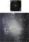 |
Fig. 1 RGB image of Holmberg II with HE red, YE green, and IE blue. Foreground extinction has been corrected and sky subtracted as described in the text (Sect. 4.1). In the top panel, the full FoV of 0.7 × 0.7 is shown, while the bottom panel displays the inner 6’ × 6 ’ region corresponding to the white box in the upper panel. In the lower panel, to the east, there is an extensive north-south chain of H II regions (e.g., Hodge et al. 1994) that harbors the ultraluminous X-ray source Ho II ULX-1 (e.g., Zezas et al. 1999; Kaaret et al. 2004), visible as a triangular-shaped blue H II region at α = 08:19:28.98, δ = +70:42:19.3 (J2000). Also visible as a blue circular structure to the north of the H II-region chain is an artifact dichroic ghost (see also Sect. 6, Fig. 15). |
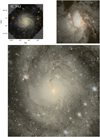 |
Fig. 2 As in Fig. 1, but for IC 342, and with the top left panel showing the full FoV of 0.7 × 0.7 and the bottom panel showing the inner 6’ × 6’ region corresponding to the white box in the upper left. The top right panel shows the zoomed-in 30ʺ × 30ʺ RGB image of the blue nucleus, also revealed in the radial color profiles (see Sect. 4.4, Fig. 6). |
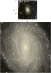 |
Fig. 3 As in Fig. 1, but for NGC 6744, the most distant galaxy of the Showcase. In the top panel, the full FoV of 0.7 × 0.7 is shown, while the lower panel gives the inner 6’ × 6 ‘ region corresponding to the white box in the upper panel. The filamentary dust lanes within the spiral arms are delineated with exquisite detail. |
4.2 Comparison of stellar and HI morphologies
Stellar content and H I gas properties are intimately related. In luminous galaxies not dominated by dark matter (DM), the stars dominate the gravitational potential (e.g., van der Kruit 1981; Mancera Piña et al. 2022), and for galaxies of all types, the combination of stars and H I is fundamental for determining the characteristics of the DM. It is commonly thought that H I gas tends to be more extended than the stellar disk (e.g., Bosma 2017), possibly because of dwarf galaxy satellites being disrupted in the process of a minor merger (e.g., Kamphuis & Briggs 1992; Mayer et al. 2006; Boselli et al. 2014; Žemaitis et al. 2023), or through cold accretion episodes (e.g., Bland-Hawthorn et al. 2017), or both. However, deep optical imaging suggests that stellar substructures can extend as far as the H I disk (e.g., Lewis et al. 2013; Okamoto et al. 2015). Recent work on HI demographics finds that the extent of the H I disk depends on star-formation activity, and that more massive galaxies tend to have less extended H I disks (Reynolds et al. 2023). The extent of HI also depends on environment, since there is a decrease in the H I-to-optical diameter in cluster environments (e.g., Reynolds et al. 2022).
Here, for illustration, in Fig. 4 we compare the H I morphology in IC 10 and IC 342 to the stellar content as traced by Euclid imaging6. The HI data for IC 10 are taken from Wilcots & Miller (1998)7, and for IC 342 from Chiang et al. (2021). The beam sizes are shown in the lower-left corner of the overlays; 1σ sensitivities range from ~1.3 × 1018 cm-2 for IC 10 (bottom panel), to 1 × 1019 cm-2 for IC 10 (top), and ~2 × 1020 cm-2 for IC 342 (middle). It can be seen from Fig. 4 that the stars in IC 10 are slightly more spatially extended than this HI map, although the HI feature to the south is not reflected in the Euclid IE morphology. The outer H I spiral arms in IC 342 do not fall within the stellar disk, but the bulk of the H I distribution is closely mirrored by the stars. The Euclid IE ‘spur’ toward the northwest is not seen in the H I morphology tracing spiral arms in the gas.
Measurement sensitivity in terms of H I beam size and limiting column density, and the SB limits that can be achieved for the stellar component, are arguably the most important discriminators for determining the relative sizes of the H I and stellar distributions (e.g., Xu et al. 2022). The bottom panel of Fig. 4 shows an HI moment map taken from Namumba et al. (2019) with a larger beam than that shown in Fig. 4 (top panel). With this larger beam, sensitive to fainter H I column densities, the H I extends beyond the stellar disk, extending to the northwest where there is a putative stellar stream culminating beyond the Euclid FoV (e.g., Nidever et al. 2013; Namumba et al. 2019). We examine whether this extension seen with Euclid can be associated with stars or foreground cirrus in the next section. In any case, the above comparison demonstrates that the interplay of stars and H I morphology in galaxies can be reassessed on a statistical basis with the sensitivity of Euclid.
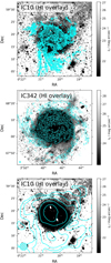 |
Fig. 4 HI overlays on high-contrast Euclid IE images: IC 10 (top panel); and IC 342 (middle). The H I beam size is shown in the lower left corner, and contours are at 2σ, 4σ, 7σ, 10σ, and 20σ. The bottom panel gives the H I overlay for IC 10 as in the top panel, but using the 3-arcmin beam-smoothed H I image from Namumba et al. (2019); contours are at 2σ, 3σ, 5σ, 10σ, 10σ, and 70σ. |
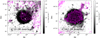 |
Fig. 5 Herschel SPIRE 250 μm overlays on high-contrast Euclid IE images for IC 10 (left panel) and IC 342 (right). |
4.3 Comparison of stellar, ISM, and cirrus emission
Atomic gas and dust tend to be spatially correlated within a typical ISM. However, in nearby galaxies it is not always straightforward to separate the foreground dust emission in the Milky Way (MW) from dust emission originating within the nearby galaxy itself. Conversely, H I enables such a separation because of the spectral resolution and corresponding velocity measurements. Figure 5 overlays far-infrared (FIR) dust emission from Herschel SPIRE/250 μm over high-contrast Euclid IE images of IC 10 and IC 342. The FIR images are taken from the Dwarf Galaxy Survey (Madden et al. 2013) and the Key Insights on Nearby Galaxies: A FIR Survey with Herschel (Kennicutt et al. 2011).
The dust emission in IC 10 roughly follows the IE filament to the northwest, but it is not altogether possible to distinguish the dust morphology from thatoftheHI gas shown in Fig. 4 (bottom panel). Although HI and dust tend to be cospatial, identifying the origin ofH I and FIR is problematic in IC 10 because of its proximity, and thus low recession velocity, relative to the MW. IC 10 has a recession velocity of -348 km s-1, so is somewhat more blue-shifted than the highest H I velocities (-150 km s-1) considered as belonging to the MW by Planck Collaboration XXIV (2011). Those authors also found that the emissivity of Galactic dust in these high-velocity clouds is low, so that relatively little dust emission would be expected from such clouds (see also Bianchi et al. 2017, who analyzed the Virgo cluster). The H I gas around IC 10 toward the northwest extension is found at about -400 km s-1 (e.g., Nidever et al. 2013), a higher velocity than expected for gas belonging to the MW, and consistent with being intrinsic to IC 10.
However, it is not clear whether the filamentary dust traced by the FIR in IC 10 belongs indeed to IC 10. The large-scale Herschel SPIRE/250 μm image suggests that there is dust emission throughout the entire northwest region around IC 10, which is more widespread than the H I, and possibly corresponding to a MW cirrus field. A stellar overdensity toward the NW could resolve the ambiguity, but there is no such obvious feature (see Sect. 5.5). Galactic cirrus tends to have blue optical colors (Román et al. 2020), but the severe foreground extinction of AV ≳ 4 toward IC 10, and its possible spatial variation, makes an accurate color determination difficult, as well as the separation of the IE stellar emission from potential cirrus, either belonging to the MW or IC 10.
In contrast, the case of IC 342 is unambiguous. Dust emission toward IC 342 follows the IE emission in the spur feature, but the H I at the recession velocity of IC 342 does not. The conclusion is that in IC 342, the IE emission in the spur is due to foreground cirrus, rather than a stellar stream. Its morphology is mirrored exactly by the FIR 250 μm-emission, but not in H I. Consequently, in addition to tracing stars, sensitive Euclid IE images, compared with other wavelengths, will be a powerful diagnostic for the Galactic ISM, in particular for assessing the importance of the diffuse cirrus component.
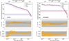 |
Fig. 6 Top: Surface brightness profiles and color profiles extracted by AutoProf as described in the text for IC 342 (left panel) and NGC 6822 (right). Upper panel: SB radial profiles for IE, YE, JE, and HE . The four bands are shown as purple, blue, green, and red curves for IE, YE, JE, and HE, respectively. The 1σ SB limits from AutoProf (not rescaled to 100 arcsec2 regions) in units of mag arcsec-2 are shown as dashed horizontal lines, with colors corresponding to the Euclid bands. The fluxes have been corrected for foreground extinction (see Sect. 4.1); the uncorrected IE profile is shown as a dotted (purple) curve in the top panel. Middle and bottom: IE - HE and YE - HE radial color profiles. The top axis corresponds to galactocentric radii in units of arcsec, and the bottom in units of kpc. The mean IE - HE color over typically a factor of 100 in radius is shown as a horizontal dashed line in the middle panel; the light gray rectangular regions illustrate the full spread in model colors (see Fig. 7) and the dark gray one the standard deviation about the mean of the models. The mean galaxy IE - HE with its standard deviation is also shown as a gray rectangular region in Fig. 7. |
4.4 Surface brightness profiles
We generated surface brightness profiles for the Showcase galaxies using AutoProf. AutoProf is a Python-based pipeline for nonparametric profile extraction, and includes masking, sky determination, centroiding, and isophotal fitting (Stone et al. 2021). For this paper, we used AutoProf in the default mode but with 5σ clipping. Because centers are difficult to determine, particularly in nearby dwarf galaxies with resolved stellar populations, we fixed the profile centers to the NED coordinates for the galaxy. Results are shown in Fig. 6 for IC 342 and NGC 6822; the profiles of the remaining galaxies appear in Fig. C.1. The sky values determined from Approach (2), as given in Table A.1 and shown in Fig. A.2, are consistent to within afew percent with the sky levels from AutoProf.
In Fig. 6 (and Fig. C.1), the surface brightness profiles corrected for foreground extinction are shown as solid lines, while for IE the uncorrected profile is shown as a dotted line. Because of their low Galactic latitude (see Table 1), for IC 10, IC 342, and NGC 6822, these corrections can be significant, up to 3 IE mag in the case of IC 10. The top horizontal axis reports the angular galactocentric distance, while the bottom gives the physical radii in kpc. Figures 6 and C.1 show that in these nearby galaxies Euclid is able to trace galaxy emission out to 20-30 kpc in radius in a single ROS.
Figures 6 and C.1 also illustrate the difficulty of determining the sky value when the galaxy fills the image. The profile of IC 342 extends smoothly out to the limits of the Euclid FoV (1600ʺ on the diagonal), but does not quite achieve the SB limits expected from Sect. 3.2. The implication is that the galaxy emission could have been measured at even larger radii were it not limited by the (already large) FoV. On the other hand, the profile of NGC 6822, an apparently smaller galaxy, approximates the SB limits in the very outer regions. The problem of large galaxies will be mitigated in the EWS, because of its more continuous coverage.
4.5 The diagnostic power of Euclid colors
The radial trends of selected Euclid colors, IE - HE and YE - HE are also shown in Figs. 6 and C.1. As an initial evaluation of the photometric calibration (see also Sect. 5), we compare the colors of the Showcase galaxies with those obtained using synthetic templates. In particular, we use Bruzual & Charlot (2003) synthetic models, and calculate the magnitudes using the SED- fitting code lephare (Arnouts et al. 1999; Ilbert et al. 2006). We assume an exponentially declining SFH, with an SFR duration τ in the range 0.1-30 Gyr, ages up to 14Gyr, metallicity from subsolar to solar (0.2 Z⊙, 0.4 Z⊙, and Z⊙), and vary the internal extinction with E(B - V) = 0, 0.1, 0.2, and 0.3 using the attenuation curve of Calzetti et al. (1994). From the combination of these parameters, we generate a library of 2300 synthetic magnitude sets at z = 0. Given the wide range of parameters explored, most of the galaxies in the local Universe would be expected to possess colors within the model predictions.
From the distribution of the Euclid colors in the library, we determine the median and the 16-84th quantile of the distributions, and find the following color ranges: IE - YE = 0.45 ± 0.24; YE - JE = 0.10 ± 0.08; and JE - HE = 0.09 ± 0.09. In Figs. 6 and C.1, these are shown as dark gray rectangular regions. The full color ranges spanned by the models are encompassed by the light gray ones.
Virtually all of the colors shown in Figs. 6 and C.1 fall within the ranges predicted by these models. In the spirals, IC 342, NGC 2403, and NGC 6744, there is a trend for the outer regions to be bluer than the bulk of the inner disk, possibly implying an inside-out disk formation scenario (e.g., Williams et al. 2009b; Gogarten et al. 2010; Wang et al. 2011), consistent with radial metallicity gradients in nearby spirals (e.g., Sánchez et al. 2014) Conversely, the central regions ofIC 342 and IC 10 are extremely blue, challenging the spread of allowable colors predicted by the models. However, as shown in Figs. 2 and B.1, the centers of both galaxies are unusual. IC 342 has an extremely luminous young star cluster complex in its nucleus (Böker et al. 1999; Carson et al. 2015; Balser et al. 2017), the brightest of those examined by Carson et al. (2015). Figure 2 and HST colors show that it is extremely blue, associated with a massive H II region and an X-ray source (Mak et al. 2008). In IC 10, the NED center position corresponds to a complex of H II regions (e.g., Hodge & Lee 1990; Polles et al. 2019), and there are several more located near the nucleus (e.g., Vacca et al. 2007). Thus, extremely blue nuclear colors are expected for both IC 342 and IC 10.
We explore this further in Fig. 7, where IE - HE is plotted as a function of age, and color coded by metallicity Z. We compare the predictions of the Bruzual & Charlot (2003) models described above and shown in the left panel, with those of Bruzual & Charlot (2003) for single stellar population (SSP) models and with PEGASE SSPs by Fioc & Rocca-Volmerange (1997) and Le Borgne et al. (2004). No internal extinction has been applied to the SSP colors. Also shown as gray regions are the mean IE - HE color ranges of the Showcase galaxies that are reported as horizontal dashed lines in Figs. 6 and C.1. The models in the left panel of Fig. 7 were generated with a limited range of metallicities and ages, as can be seen from the comparison with the SSPs in the right two panels. In addition to the different parameter ranges, the BC03 models behave differently due to the smoothed-out SFH in the left panel, compared to the SSP in the middle one. The BC03 and PEGASE SSP models also differ in their treatment of red supergiants (RSGs) that begin to dominate at ~10 Myr, and the most massive asymptotic giant branch (AGB) stars at -100 Myr.
The bluest colors are found at young ages, ≲ 10 Myr, consistent with the properties of IC 10 and IC 342 in their central regions. Moreover, subsolar metallicity makes these colors even bluer, so appropriate for IC 10 at about 0.3 Z⊙ (log10(Z/Z⊙) = -0.55 for the color coding). At a slightly super-solar metallic- ity, the age of the IC 342 nuclear star cluster is estimated to be ~ 5 Myr (e.g., Carson et al. 2015), so the limits of the SSP PEGASE models constrain well the observed colors at this young age.
In summary, Euclid colors are diagnostic of the age and metallicity of the stellar populations in galaxies, and will provide an important tool for the exploration of broader galaxy populations. At Euclid’s resolution, in the centers of these nearby galaxies, we are essentially just probing small star clusters or even bright stars. At the same time, Euclid’s sensitive SB limits allow the examination of galaxy disks to depths that can reveal disk breaks and faint external features of galaxies that could be signatures of interaction (e.g., Peters et al. 2017; Sánchez-Alarcón et al. 2023). Details of the SB profiles and color gradients, and the disk properties of the Showcase galaxies, will be discussed in a future paper.
 |
Fig. 7 Synthetic IE - HE from the Bruzual & Charlot (2003) models with exponentially declining SFH (left panel); the same Bruzual & Charlot (2003) models but SSPs (middle); and PEGASE SSP models from Fioc & Rocca-Volmerange (1997, right) and Le Borgne et al. (2004). The SSP models have no internal extinction applied to the colors. Also shown as gray regions are the mean IE - HE colors and their standard deviations, as reported in the middle panel of Figs. 6 and C.1, evaluated over a factor of 100 in galactocentric radius. As discussed in Sect. 4.1, these colors have been corrected for foreground extinction from our Galaxy. The different behavior of the models is due to the smoothed-out SFH in the left panel, and the different treatment of red supergiants that begin to dominate around 10 Myr, and the most massive AGB stars around 100 Myr. |
5 Resolved stellar photometry and star counts
Going beyond the integrated light described in Sect. 4, photometry of resolved stars in nearby galaxies is a powerful tool, not only for understanding stellar content and galaxy formation scenarios, but also for probing the outer regions of galaxy disks and disk formation (e.g., Barker et al. 2012; Crnojevic’ et al. 2016; Hillis et al. 2016; Jang et al. 2020a). The surface brightness of resolved stellar populations, once corrected for completeness and projection effects, can reach fainter SB limits than integrated light alone (e.g., Barker et al. 2012). Thus, through stellar photometry in nearby galaxies, Euclid opens a new perspective also on resolved stellar populations and their diagnostic capabilities. Here we present a first look at resolved stellar photometry in the Showcase galaxies.
5.1 Stellar photometry
For all galaxies, point-source photometry was performed with SourceExtractor (Bertin & Arnouts 1996). Detections were considered independently in the four Euclid bands, adopting a 7 × 7 mexhat (wavelet) filter before detection, and then considering as valid detections all sources having even a single pixel 1.5σ above the background. The filtering step performed by SourceExtractor prior to source identification has the effect of “smoothing” the images, thus minimizing spurious detections despite the low 1.5σ detection threshold. The photometric analysis of the identified sources is performed on the original images. For the photometry, we adopted a 5-pixel diameter aperture, corresponding to 0ʺ.5 and 1ʺ.5 in the VIS and NISP images, respectively. This aperture, which totals approximately 3 times the PSF FWHM in all Euclid bands, is sufficiently small to guarantee accurate photometry in moderately crowded regions of the galaxies. Aperture corrections from 5-pixel to large apertures of 6ʺ for VIS and 18ʺ for the NISP images, totaling about 40 times the FWHM of the PSFs, were computed from the most isolated, bright, unsaturated stars. The corrections amount to -0.27, -0.11, -0.12, and -0.15 mag in IE, YE, JE, and HE, respectively. Finally, magnitudes were calibrated applying the zero points of ZPIE = 30.13, and ZPNIR = 30.0, as discussed in Sect. 3. PSF- fitting photometry aimed at characterizing the resolved stellar content of the innermost star-forming regions will be presented in subsequent papers.
The photometric catalogs in the VIS and NISP bands were cross-matched by assigning a 1ʺ maximum tolerance in separation between sources. For every galaxy except IC 342 and NGC 6744, we were able to produce a final master catalog con-taining only sources with photometric detections in all four bands. For IC 342 and NGC 6744, in order to achieve sufficient statistics, we adopted a less conservative approach, and crossmatched the IE VIS band with only the JE and HE NISP bands. Although comparable depth is reached by all the NISP bands (namely, YE =24.45, JE =24.6, HE =24.5 at 5σ for a point source, Cuillandre et al. 2025), the YE band is less advantageous than the JE or HE bands for detecting faint red RGB stars or stars that suffer significant extinction. In any case, the cross-match removes the majority of spurious detections, such as cosmic rays, emission peaks on bright star spikes, or residual artifacts from the image reduction pipeline described in Sect. 3.
Additional selection cuts based on some of the SourceExtractor output parameters are then applied to remove saturated stars and extended background galaxies. More specifically, we retain sources that: (i) have a measured FWHM in VIS between 1.2 and 2.5 pixels; and (ii) lie within the locus populated by compact sources in the plane defined by central surface brightness (μmax) versus aperture magnitude, as illustrated in Fig. 8. Objects with a FWHM smaller than 1.2 pixels (namely smaller than the PSF) are likely artifacts, while values of the FWHM larger than 2.5 pixels have a high probability of being associated with extended objects. Indeed, extended systems (such as background galaxies or resolved star clusters), as well as saturated stars, tend to have fainter central surface brightnesses compared to point sources with the same aperture flux. Nevertheless, such selection criteria are not always effective in removing very compact background galaxies from the final catalog. The horizontal concentration of sources at FWHM(IE)=10 in the top panel of Fig. 8 is due to spurious detections related to the effect of saturation, and corresponding NaN pixels. With these cuts, we are left with: 332 900, 323 260, 116 551 and 30 755 sources in the IE-YE-JE-HE matched catalogs of NGC 6822, IC 10, NGC 2403, and Holmberg II, respectively; and 318 366 and 162 286 sources, respectively, in the IE-JE-HE matched catalogs of IC 342 and NGC 6744.
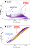 |
Fig. 8 SourceExtractor output parameters for NGC 6822, intended to illustrate the typical selection cuts applied to our photometric catalogs. Purple points are the sources matched in all four Euclid bands, while yellow points correspond to our selections. In the top panel, we retain all sources with a measured FWHM in VIS of between 1.2 and 2.5 pixels, while in the bottom panel, we show our adopted selection in the plane defined by central surface brightness versus aperture magnitude. Sources with a FWHM smaller than 1.2 pixels (namely smaller than the PSF) are likely artifacts, while sources with large FWHM values and/or large values of μmax compared to aperture photometry are either saturated stars or extended objects (background galaxies or resolved star clusters). |
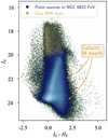 |
Fig. 9 IE versus IE-HE color-magnitude diagram of all sources within the FoV of NGC 6822 after applying the selection cuts described in Sect. 5.1 and illustrated in Fig. 8 and after correction for foreground extinction (Sect. 5.2). Yellow points indicate bright MW and background galaxy contaminants, namely sources cross-matched with the Gaia DR3 catalog that have a measured proper motion PM larger than 3σPM. The vertical feature at IE - HE ≃ 1.3, IE ≳ 21 is due to the M dwarf population of the MW. |
5.2 Reddening correction
Individual source magnitudes were corrected for spatially variable foreground reddening, as described in Sect. 4.1, but for each source position, rather than assuming a single value for the entire galaxy. Also, rather than using a flat spectrum as for the integrated light, here we assume a 5700 K blackbody to approximate a G2V stellar spectrum in order to better emulate the emission from individual stars. This assumption provides relative ratios of Aλ/AV=0.726, 0.375, 0.266, and 0.173 for IE, YE, JE, and HE, respectively. The correction is modest in the case of Holmberg II, NGC 2403, and NGC 6744, while it has a major impact on the CMDs of IC 10, IC 342, and NGC 6822, which suffer the strongest extinction. Indeed, the reddening-corrected CMDs of these galaxies exhibit, besides a global shift toward brighter magnitudes and bluer colors, narrower and cleaner stellar evolutionary sequences compared to the noncorrected CMDs.
5.3 Foreground star removal
Although the selection cuts described in Sect. 5.1 are effective in removing a substantial fraction of extended background galaxies, our photometric catalogs still suffer from major contamination due to foreground Galactic stars. This is evident in Fig. 9 where we show, as an illustrative example, the final calibrated, reddening-corrected IE versus IE - HE CMD of NGC 6822. In the diagram, the vertical band of sources delineating a sharp edge at IE - HE ≃ -0.4 and extending toward the red up to IE - HE ≃ 1.3 are main sequence stars from the Galactic disk, with the vertical feature at IE - HE ≃ 1.3, IE ≳ 21 due to the M dwarf population. In order to remove these contaminants, we adopt two complementary steps using (i) the constraints provided by Gaia proper motions (PMs), and (ii) the implementation of additional selections based on color-color diagrams in the Euclid bands.
In step (i), we cross-correlate our photometric catalogs with the Gaia DR3 release (Gaia Collaboration 2021), adopting a 1ʺ maximum tolerance in RA, Dec coordinates. Since the ERO Showcase galaxies have PMs compatible with zero within the errors (e.g., McConnachie et al. 2021; Bennet et al. 2024), likely MW members are identified, and then removed from our catalogs, as those having a measured proper motion PM larger than 3σPM, where σPM is the PM uncertainty. With this approach, we effectively remove bright foreground stars with IE ≲ 20 from our CMD. The removed sources are indicated as yellow points in the CMD of Fig. 9. Nonetheless, it is evident that the vertical sequence of MW contaminants at IE - HE 0.4 and IE ≳ 20 is still present in the CMD.
Next, we implement step (ii) to remove some foreground contaminants fainter than IE - 20, which do not have a counterpart in Gaia. More specifically, we apply a selection in the YE - HE versus IE - HE plane, as shown in Fig. 10 for NGC 6822. As illustrated in the top panel of the figure, stars in the MW and in NGC 6822 populate the same locus of the diagram at IE - HE ≲ 1, because the colors of giant and dwarf stars are degenerate for early spectral types. Indeed, stellar isochrones (Bressan et al. 2012; Marigo et al. 2017) displayed for a wide range of ages (10 Myr to 10 Gyr) and metallicities of ≲40% solar8, compatible with NGC 6822’s chemical abundance estimates (Venn et al. 2001; Lee et al. 2006; Patrick et al. 2015), completely overlap at blue colors with the TRILEGAL model of the Milky Way (Girardi et al. 2005, 2012), so that a separation between the two components is not possible in this regime. On the other hand, the colors of dwarf and giant stars start to diverge at IE - HE ≳ 1, and Galactic M dwarfs depart from giants in NGC 6822, forming a relatively bluer sequence with -0.15 < YE - HE ≲ 0.3 (see e.g., Majewski et al. 2003; Bentley et al. 2019, for similar classifications). The selection outlined in the bottom panel of Fig.10 therefore provides a sensible strategy for the removal of a large number of MW M-dwarf contaminants. M dwarfs belonging to NGC 6822 are not present in our catalog because, at the galaxy distance of 0.5 Mpc, they are too faint to be detected.
The selection illustrated in Fig. 10 also enables the removal of a few residual spurious detections (typically located at the edge of detectors) and the contribution from compact red galaxies that survived the initial cuts based on the SourceExtractor parameters in Sect. 5.1; these sources have IR colors typically redder than Galactic M dwarfs (see, e.g., Fig. 2 of Bell et al. 2019) and form a separate sequence with YE - HE colors intermediate between those defined by Galactic M dwarfs and AGB stars in NGC 6822. A visual inspection of these sources in the VIS image confirms that they are compact background galaxies. Indeed, although a portion of the isochrones displayed in red in the top panel of Fig. 10 seems to closely follow that intermediatecolor sequence of sources, we checked that both the position of these sources on the CMD of NGC 6822, and their rather uniform distribution over the FoV, excludes their association with NGC 6822. Furthermore, a direct visual inspection on the VIS image clearly reveals that they are either compact background galaxies or the nuclei of relatively more extended ones.
After removal of MW contaminants, we are left with 233 900, 199260, 65 296, and 16928 sources in the IE-YE- JE-HE matched catalogs of NGC6822, IC10, NGC2403, and Holmberg II, respectively; and with 120 747 and 112 872 sources, respectively, in the IE-JE-HE matched catalogs of IC 342 and NGC 6744. The surviving stars after removal of these contaminants are typically 56-70% of the original sample. The exception is IC 342, where the fraction drops to 38% due to the high foreground star contamination for this low-Galactic latitude galaxy, coupled with its relatively large distance (see Table 1), which hampers the detection of its resolved stellar population.
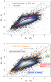 |
Fig. 10 Distribution in the YE - HE versus IE - HE plane of sources in the NGC 6822 photometric catalog after removal of bright IE ≲ 20 MW disk stars in Gaia DR3. In the top panel, the PARSEC stellar isochrones (Bressan et al. 2012; Marigo et al. 2017) in the Euclid bands are superimposed in red for different ages (from 10 Myr to 10 Gyr) and metallicities of Z ≲ 0.006 (about one-third solar); the TRILEGAL Galaxy model is shown in blue. Giant stars in NGC 6822 and dwarf stars in the MW overlap at IE - HE ≲ 1, while the two populations diverge at redder colors. In the bottom panel, we denote the location of Galactic M dwarf stars, AGB stars in NGC 6822, background compact red galaxies, and residual spurious detections. The dashed orange polygon outlines our final selection, which provides a reasonable compromise between the need to retain the largest possible number of stars belonging to NGC 6822, while removing Galactic M dwarfs, compact red galaxies, and residual spurious detections (see text for details). |
 |
Fig. 11 CMDs of the final calibrated reddening-corrected photometry for NGC 6822, after removal of extended background galaxies, bright MW contaminants and faint Galactic M dwarf stars. Left panel: IE versus IE - HE . The main stellar evolutionary sequences are indicated: the blue plume (BP), populated by massive MS and post-MS stars in the hot core helium-burning phase (ages ≲ 100 Myr); RSGs with ages from about 20Myr to 50 Myr; bright and red AGB stars with ages from 0.1 to 2 Gyr; red giant branch (RGB) stars, with ages older than 1-2 Gyr; the red clump (RC) of low-mass stars in the core-helium burning phase; and the AGB bump (AGBb). The blue, green, and red polygons, driven by the comparison with stellar evolutionary models, indicate the selection regions used to create the star count maps in Sect. 5.5. as indicated in the legend. Middle: IE versus IE - HE (same as left panel) with superimposed PARSEC stellar isochrones for different ages (10 Myr to 10 Gyr) and for two metallicity values, Z = 0.006 and 0.001 (40% and 6% solar, respectively.). Right: JE versus YE - HE. In this diagram, the oxygen-rich and the carbon-rich AGB stars (O-AGB and C-AGB) appear well separated and define vertical and horizontal sequences, respectively. |
5.4 Identifying individual stellar populations
To illustrate the results, we show in Fig. 11 the final IE versus IE - HE and JE versus YE - HE CMDs of NGC 6822. These diagrams present a dramatic improvement when compared to the CMD of Fig. 9, since the removal of foreground and background contaminants unveils the presence of well-defined stellar evolutionary sequences within NGC 6822, which are indicated in the left panel of Fig. 11: a blue plume (BP) at -2 ≲ IE - HE ≲ -1, populated by massive main sequence (MS) stars and post-MS stars in the hot core helium-burning phase, with ages ≲ 100 Myr; a vertical sequence of RSGs at IE - HE ≃ 1, 17.5 ≲ IE ≲ 19.5, with ages from about 20 Myr to 50 Myr; bright and red (1.2 ≲ IE - HE ≲ 5) AGB stars with ages from about 0.1 to 2 Gyr; and red giant branch (RGB) stars with 0 ≲ IE - HE ≲ 1.5, IE ≳ 20 and ages older than 1-2 Gyr (and potentially as old as ~13 Gyr). Also visible at -0.4 ≲ IE - HE ≳ 0.6, IE ≳ 23.5, towards our detection limit, is the red clump (RC) of low-mass stars in the core-helium burning phase, with ages >1-2 Gyr. At IE - HE ≃ 0.3, IE ≃ 22.7 we detect the AGB bump (AGBb).
A direct comparison between the observed CMD and the predictions of stellar models is presented in the middle panel of Fig. 11, where we overplot the PARSEC stellar isochrones (Bressan et al. 2012; Marigo et al. 2017) in the Euclid bands for stellar ages in the range 10 Myr-10 Gyr; isochrones younger than ~1 Gyr are displayed for a Z = 0.006 metallicity (about 30% solar), compatible with estimates from H II regions or young supergiants in NGC 6822 (Venn et al. 2001; Lee et al. 2006; Patrick et al. 2015), while a lower metallicity of Z = 0.001 is adopted for older populations. The models were shifted by applying a distance modulus of (m - M)0 = 23.54 from Fusco et al. (2012), corresponding to a distance of 510 kpc. This distance is compatible with the observed RGB tip (TRGB) at IE ≃ 20.2. Indeed, a recent calibration of the TRGB in the Euclid bands based on Gaia-DR3 synthetic photometry predicts an absolute value of MIE,TRGB = -3.3 (Bellazzini & Pascale 2024) that translates into a distance modulus of 23.5 in IE, consistent with the distance from Fusco et al. (2012), but somewhat larger than the 470-kpc distance found by Weisz et al. (2014).
The right panel in Fig. 11 presents the JE versus YE - HE CMD of NGC 6822. In this CMD, the same stellar evolutionary sequences described for the IE versus IE - HE CMD can be easily identified, with the exception of the less evident RC and AGBb features. On the other hand, there is a clearer separation between O-rich versus C-rich AGB stars, with the former delineating an almost vertical sequence with colors 0.35 ≲ YE - HE ≲ 0.55, and the latter forming a horizontal feature at 17.9 ≲ JE ≲ 18.5 (see also Nally et al. 2024, for a similar classification based on JWST data).
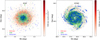 |
Fig. 12 Maps of star counts of two Showcase galaxies divided into individual stellar populations as described in the text: IC 10 (left panel); and IC 342 (right). Young stars are shown as blue points, AGB stars as green, and evolved RGB stars as red. More details are given in the text. In IC 10 (left panel), young stars are clearly more concentrated than the older ones, and in IC 342 (right), the young stars clearly delineate the spiral arms out to large galactocentric radii. |
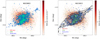 |
Fig. 13 Star-count maps obtained as for Fig. 12, but for the closest Showcase galaxy, NGC 6822 (left panel), and with HI contours overlaid on the maps (right). HI data are taken from de Blok & Walter (2000); contours are at 2σ, 4σ, 7σ, 10σ, and 20σ. The young stars in NGC 6822 are clearly aligned with the atomic gas, as discussed in the text. |
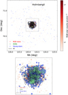 |
Fig. 14 Star-count maps obtained as for Fig. 12, but for Holmberg II with H I contours overlaid (top panel); the bottom panel shows the zoomed-in image corresponding to the 15’ × 15’ gray box (shown in the top panel). H I data are taken from Walter et al. (2008); contours are at 2σ, 4σ, 7σ, 10σ, and 20σ. The AGB and old RGB stars are not visible in the map of Holmberg II because they are entirely covered by young stars. |
5.5 Star-count maps
The features outlined by the polygons in the left panel of Fig. 11 were used to select stellar populations for different age intervals in the six Showcase galaxies. These selections were slightly adapted to account for the different depths sampled, depending on the galaxies’ distances. The age selection thus enabled the construction of star count maps in different age intervals.
The final maps were smoothed by convolving with a Gaussian kernel the two-dimensional histograms. Subtraction, in a statistical sense, of foreground stars or background objects that do not belong to the galaxies was performed by removing the density of counts computed in regions at large galactocentric distance, where it is reasonable to assume a negligible presence of the intrinsic stellar populations from the galaxy. However, this may lead to an over subtraction of the background in the case of NGC 6822, for which Zhang et al. (2021) demonstrated that the stellar component extends at faint levels to beyond the Euclid FoV. The star counts within these regions were calculated, together with their standard deviation, σbck. The final maps were constructed by only considering the star counts that exceeded σbck by a given signal-to-noise: S/N = 5 for young stars; and S/N = 3 for RGB and AGB stellar populations, in order to better highlight low surface brightness structures in the old stellar component.
The stellar populations in the Showcase galaxies will be examined in detail in future papers, with a careful analysis of completeness limits, local extinction corrections, and galaxy membership. Here, we present the results of the preliminary analysis described above. Figure 12 shows smoothed maps of the star counts for IC 10 and IC 342, while NGC 6822 is presented in Fig. 13, and Holmberg II in Fig. 14. The remaining maps can be found in Appendix D; we have obtained star counts with Euclid even for NGC 6744, which has the largest distance in the Showcase sample (9 Mpc), although there we mostly detect young stars, AGB stars, and blends of bright RGB stars.
The maps of the giant spirals, IC 342 and NGC 6744, show that young stars follow closely the spiral structure well into the outer disk, exemplifying the notion that spiral arms tend to be the sites of recent star formation (e.g., Gerola & Seiden 1978; Roberts & Hausman 1984; Wada et al. 2011). Similar behavior is also seen in M 33, a flocculent spiral (Lazzarini et al. 2022), M81 (Williams et al. 2009a; Okamoto et al. 2015), and NGC 6946 (Tran et al. 2023). The AGBs in IC 342 also follow the spiral arms, but tend to be more broadly distributed, possibly implying the lack of a systematic time delay in the SFH across the arm, similar to the case ofM 81 (e.g., Choi et al. 2015).
Conversely, rather than tracing the flocculent spiral structure, the young stars in NGC 2403 (see Appendix D) are more uniformly distributed across the disk (see also Barker et al. 2012). This would imply that the young stellar disk in NGC 2403 has been relatively undisturbed out to a galactocentric radius >10 kpc, similar to its morphological twin, NGC 300 (e.g., Hillis et al. 2016; Jang et al. 2020b).
Figures 12 and 13 show that in the dwarf galaxies, IC 10 and NGC 6822, the AGB stars are more centrally concentrated than the RGBs, a common (e.g., Gerbrandt et al. 2015), but not inevitable (e.g., Bernard et al. 2012), feature in dwarf irregular galaxies (see e.g., Fig. 14). It is more difficult to characterize the stellar populations in IC 10 than the other galaxies in the Showcase, because of large foreground extinction and contamination by foreground stars (e.g., Massey et al. 2007). We find that the stellar distribution in IC 10 is quite extended in roughly a circular morphology (see also Fig. 4), consistent with Gerbrandt et al. (2015). The young-star counts are even more centrally concentrated than the AGB stars, with the AGB stars possibly showing more of a flattened distribution in the central regions. It is interesting to speculate that this feature could be a signature of a past star-formation event. According to Weisz et al. (2014), in IC 10, like other dIrr galaxies, significant star formation has taken place over the last 2-3 Gyr; some of these stars are most likely the progenitors of the AGB population in IC 10 (see also Dell’Agli et al. 2018). Maps of the atomic gas (see Fig. 4) suggest that IC 10 has undergone an interaction in the past, or is currently accreting gas (e.g., Shostak & Skillman 1989; Nidever et al. 2013; Ashley et al. 2014; Namumba et al. 2019).
The configuration and orientation of the RGB and AGB populations in NGC 6822 shown in Fig. 13 agree with previous maps (e.g., Demers et al. 2006; Sibbons et al. 2012; Tantalo et al. 2022). In NGC 6822, the young stars are oriented roughly along the H I emission, as illustrated by the overlay of H I in the right panel of Fig. 13. Young stars are found where the HI has higher column density, but are also present in the H I cavities, such as the ‘hole’ toward the southeast of the nucleus. This orien-tation of the young population was also found previously (e.g., Komiyama et al. 2003; de Blok & Walter 2003; Zhang et al. 2021), implying that high H I column density may foster star formation. However, NGC 6822 is kinematically complex, with a potentially counter-rotating component both in the gas and the stars (e.g., de Blok & Walter 2006; Belland et al. 2020), so the connection of the H I with star formation may also be influenced by kinematics. Figure 13 shows that the combined stellar morphology produces an ‘X’-like configuration of the overall stellar content, with the young stars oriented along a NW-SE direc-tion, like the H I, and the older RGBs elongated along a NE-SW direction; such a configuration is consistent with that found in previous studies (e.g., Komiyama et al. 2003; de Blok & Walter 2003; Zhang et al. 2021). There is still debate about whether the unusual properties of NGC 6822 have been caused by a prior merger or stellar feedback (e.g., de Blok & Walter 2000; Demers et al. 2006; Cannon et al. 2012; Belland et al. 2020; Zhang et al. 2021), but the case of NGC 6822 illustrates the potential of Euclid to contribute to this debate.
Figure 14 presents the star-count maps of Holmberg II, where the bottom panel gives a zoomed-in region with the H I overlay (Walter et al. 2008), corresponding to the 15’ × 15’ box shown in the top panel. Unlike most dwarf galaxies, the AGB stars in Holmberg II are not more concentrated than the more evolved RGB stars (e.g., Bernard et al. 2012). Confirming earlier work, we find that the young stellar and AGB populations are roughly spatially coincident, together with the underlying older, RGB, population. The comparison of stellar populations with the well- defined H I cavities also shows that multiple stellar populations tend to be found within the H I holes, in agreement with previous results (e.g., Puche et al. 1992; Rhode et al. 1999; Weisz et al. 2009). The implication is that a single episode of star formation is not responsible for carving the HI cavities, but rather feedback from SNe over time from multiple stellar generations. In summary, Euclid will be a powerful tool for further constraining the past history of IC 10, NGC 6822, Holmberg II, and other dwarf galaxies that will be observed during its lifetime, as well as assessing the SFH of more massive disk galaxies and the origin and longevity of spiral arms.
6 Dwarf satellites around NGC 6744
The unprecedented combination of low surface brightness sensitivity, high spatial resolution with a pristine PSF, and wide-area coverage of Euclid enables the detection and characterization of the low surface brightness dwarf satellites around their host galaxies, as well as the simultaneous study of their nuclear star clusters and globular cluster systems. To demonstrate the capability of Euclid to investigate the satellite systems of nearby galaxies, we visually identified the dwarf galaxies in the Euclid Showcase fields. Here, we present some highlights for NGC 6744.
6.1 Known dwarf satellites of NGC 6744
It is common to find ensembles of dwarf satellites around nearby galaxies (e.g., Karachentsev et al. 2014). The dwarf satellite system of the host galaxy NGC 6744 was explored in the context of the ELVES (Exploration of Local VolumE Satellites) survey by Carlsten et al. (2022), which confirmed 338 satellites with absolute magnitude MV < -9 mag and central surface brightness μ0,V < 26.5 mag arcsec-2 in the vicinity (the majority within 300 kpc) of 30 host galaxies in the local volume (D < 12 Mpc). In particular, the galaxy NGC 6744 was found to have 15 dwarf satellite candidates. Of these, five were confirmed via SBF measurements (Carlsten et al. 2019) or other methods, four were rejected via SBF, and six remained unconfirmed.
6.2 Visual identification of new satellites
In the ERO Showcase field of NGC 6744, we first identified the dwarf candidates using a combination of the high-resolution VIS image and the lower resolution (by a factor of 3) VIS+NISP color image. Jafar, an on-line visualization and annotation tool that makes use of the CDS Aladin lite facility9, was used for identifying and labeling the dwarfs (see Sola et al. 2022). The use of the color image was crucial as artifacts of the optical system, the so-called ‘optical ghosts’, appear as faint small round regions (~ 10-13ʺ in diameter) in the VIS image and look very similar to dwarf galaxies. However, since they are more prominent in the VIS image than in NISP, they have a very distinctive fuzzy blue color in the image, unlike the real dwarfs (see Fig. 15).
Of the five confirmed dwarfs of Carlsten et al. (2022), only four fall in the ERO field of view and thus are also found in our Euclid NGC 6744 dwarf catalog, as shown as RGB images in Fig. 15. The second galaxy from the left is close to the edge of the image, resulting in slightly more artifacts in NISP.
The capability of Euclid to detect and characterize new populations of dwarf (satellite) galaxies is highlighted by the confirmation of a previously identified dwarf satellite candidate in this ERO field, shown in Fig. 16. This object (dw1909m6341) was previously listed by Carlsten et al. (2022) as one of six possible satellites, and was assigned a 50% likelihood of being a satellite of NGC 6744. The superior quality of the Euclid images now confirms the association with NGC 6744 as it is clearly semi-resolved. dw1909m6341 is a nucleated dwarf elliptical with an absolute IE-band magnitude of -12.2, assuming a distance of 8.8 Mpc, with an effective radius of 0.4 kpc and a surface brightness within one effective radius of 24.1 mag arcsec-2 , placing it clearly within the scaling relations of the classical dwarf regime. It is located at α = 19° 9’ 8ʺ.33, δ = -63° 41’ 7.ʺ9 (J2000), at the end of a spiral arm, and has avoided past characterization probably because of the high stellar density in this region. However, the combination of low surface brightness sensitivity and high spatial resolution of Euclid allows us to easily identify and characterize such galaxies, even in crowded regions.
6.3 Resolved stellar populations of dwarf satellites
We compare the visual appearance of the images of a known satellite, dw1906m6357 (see Fig. 15, Carlsten et al. 2022), and one of the galaxies identified by Carlsten et al. (2022) to be a background contaminant, dw1912m6351. An example of a zoomed-in image of dw1906m6357 is shown in the left panel of Fig. 17, compared with dw1912m6351 (right panel), identified as a background object based on surface brightness fluctuation measurements. The background object is shown at the same zoomed-in scale, but is characterized by unresolved stellar light. This illustrates the capability of Euclid to clearly identify satellites of massive galaxies at the distance of NGC 6744. As can be seen in Fig. 16, the stellar population of dw1909m6341 is also resolved, suggesting that this dwarf is indeed a satellite of NGC 6744.
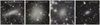 |
Fig. 15 Euclid RGB images of the four previously known dwarf satellites from Carlsten et al. (2022) that fall in the field of view of the Euclid image of NGC 6744. Red is given by HE, green by YE, and blue by IE. The sizes of the images are 250ʺ, 150ʺ, 120ʺ, and 120ʺ on a side, from left to right; north is up, east to the left. With the exception of NGC 6744A, a well-known dwarf satellite lying along spiral arms to the northwest of the nucleus, name designations are from Carlsten et al. (2022). In the cut-out of dw1906m6357 (third panel from the left), there are also two blue circular structures that are dichroic ghost artifacts (see also Fig. 1). |
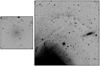 |
Fig. 16 Confirmation image of a previously identified dwarf satellite of NGC 6744, dw1909m6341; the image on the left is 50ʺ × 50ʺ. The larger 12’ ×12’ image on the right shows its location near a dense stellar region that belongs to one of the spiral arms of the galaxy. The images are oriented with north up, and east to the left. |
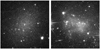 |
Fig. 17 Comparison of the zoomed-in images of one of the known satellites (left panel, dw1906m6357) shown in Fig. 15 and a galaxy (dw1912m6351, right panel) identified as a background object based on surface brightness fluctuation measurements by Carlsten et al. (2022). The sharp PSF of Euclid allows us to clearly see that the stellar population is resolved in the image on the left (satellite), but not in the image on the right (background galaxy). The images are 40ʺ on a side, with north up, and east to the left. |
7 Extragalactic globular cluster candidates in NGC 2403
The investigation of EGCs with Euclid will revolutionize our understanding of their properties, and the constraints they impose on hierarchical galaxy formation. Here we present preliminary results for the EGCs around NGC 2403, while the GC and star-cluster populations of other Showcase galaxies will be discussed in future papers (Howell et al., in prep; Larsen et al., in prep).
7.1 Known clusters and cluster candidates
The first discussion of star clusters in NGC 2403 dates back to Tammann & Sandage (1968), who presented a list of four can-didates that they had identified on photographic plates from the Hale 200-inch telescope. They noted that one of their candidates, C4, ‘could well be a globular cluster such as ω Cen or 47 Tuc’, while C1-C3 had blue colors resembling those of young star clusters in the Milky Way. A fifth object, C5, was associated with an H II region. The current list of spectroscopically confirmed old (> several Gyr) GCs in NGC 2403 consists of seven objects: C4, D6, F1, F16, F46, JD1, and JC15 (Forbes et al. 2022; Larsen et al. 2022). Objects with IDs starting with a ‘C’ are from the original list by Tammann & Sandage (1968), with a ‘D’ referring to candidates identified by Davidge (2007), and ‘F’ to Battistini et al. (1984), while clusters JD1 and JC15 were identified by Forbes et al. (2022).
The top panel in Fig. 18 shows 5ʺ × 5ʺ cut-outs from the Euclid VIS image around the seven confirmed NGC 2403 GCs. The cut-outs show that all of these clusters are resolved into individual stars in their outer parts, demonstrating Euclid’s potential for revealing additional candidates.
A number of other objects have been discussed as potential GCs in the literature. The middle panel in Fig. 18 shows the four bluer objects from Tammann & Sandage (1968). The spectra of C1 and C3 exhibit strong Balmer absorption lines, confirming these objects as young clusters, with ages of a few hundred Myr (Battistini et al. 1984; Forbes et al. 2022), while Larsen & Richtler (1998) found an age of about 250 Myr for C2 based on its UBV colors. By comparing the images of these young clusters with those of the old GCs, it is evident that morphology alone is not sufficient to identify old GCs as such. The bottom group of cut-outs in Fig. 18 shows various candidates that clearly are not stellar clusters. The spectra obtained by Forbes et al. (2022) already revealed D2 to be a foreground star. The Euclid VIS image shows that this source (as well as D3) is actually composed of two stars separated by less than 1ʺ, which explains the nonstellar appearance in the ground-based images from Davidge (2007). The VIS image also shows that D1 is a single star, while D4 is a background galaxy. None of the additional nonconfirmed GC candidates from Battistini et al. (1984) are stellar clusters. F47 has a nonzero parallax of 0ʺ.88 ± 0ʺ.12 according to Gaia DR3, which demonstrates that it is a Milky Way foreground star, while the remaining objects are background galaxies. All coordinates listed in this paper are based on the Euclid VIS astrometry10.
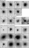 |
Fig. 18 Euclid VIS images of known GCs in NGC 2403 (top), young clusters (middle), and nonclusters (bottom). Each image shows a 5ʺ × 5ʺ cut-out around each object. North is up, and east to the left in all images. |
7.2 Searching for new clusters
Having established that the VIS images allow star clusters in NGC 2403 to be identified based on their resolution into individual stars, we carried out a search for additional cluster candidates. While we expected clusters to be identifiable from a careful, visual inspection of the images, the sheer size of the Euclid VIS image (36 000 pixels × 36 000 pixels)11 made it necessary to first apply a preselection to reduce the number of candidate sources that were then subjected to visual inspection. To this end, we first generated a source catalog by running SourceExtractor on the VIS images with relatively conservative extraction settings: DETECT_MINAREA=6 and DETECT_THRESH=8, meaning that a source detection requires six connected pixels, each with a signal of at least 8σ above the background noise. This produced an initial catalog of 392 099 sources. We also ran SourceExtractor on the NISP images, using the YE-band data for source detection while carrying out photometry on all three NISP images. The magnitudes were measured within circular apertures with diameters of 20 pixels on the VIS frame and 6.7 pixels on the NISP frames (in both cases corresponding to an aperture radius of 1ʺ), as well as in Kron-like (AUTO) apertures.
According to Cuillandre et al. (2025), the encircled energy fractions in the IE and HE filters are 0.936 and 0.883 for a point source measured in a 1ʺ aperture, corresponding to a aperture color correction of Δ(IE - HE) = 0.06. While the corrections may differ for more extended sources, we assume that a similar correction is applicable to the colors of the cluster (candidates) in NGC 2403. We verified for two clusters, D6 and F1 (which are relatively isolated), that similar color corrections are indeed obtained. Specifically, we found a mean correction of 0.05 from 1ʺ to 8ʺ for these two clusters, essentially the same value reported by Cuillandre et al. (2025) for point sources.
Next, we used the ISHAPE software (Larsen 1999) to measure PSF-corrected sizes for all sources brighter than IE(AUTO) = 22 mag. ISHAPE requires a PSF subsampled by a factor of 10 with respect to the pixel size of the VIS images, which was produced with the PSF task in the IRAF version of DAOPHOT (Stetson 1987, 1994) from about 100 stars. ISHAPE then measures the sizes by convolving the PSF with King (1962) models with a concentration parameter c = rt/rc = 30 (for tidal- and core radii rt and rc) until the best fit was obtained for each source. A list of cluster candidates to be inspected visually was then produced by applying the following selection criteria.
Magnitude: 17 < IE < 21.5.
Size: FWHM > [0.7 - (IE - 17)/10] pixels (for IE < 19) and FWHM > 0.5 pixels for 19 < IE < 21.5. Here the FWHM is the intrinsic size of the object (namely, corrected for the PSF, so that a point source should have FWHM≈0).
Color: IE - HE < 0.9 (1ʺ), or equivalently, IE - HE < 0.96 (infinite aperture).
At the distance of NGC 2403, the size cut of FWHM = 0.5 VIS pixels corresponds to a linear FWHM = 0.78 pc or a halflight radius of rh = 1.1 pc for the adopted King models. We found this cut to effectively eliminate the vast majority of individual stars, while still comfortably allowing the inclusion of GCs that have typical half-light radii ≲3 pc (Harris 1996). The magnitude-dependent size cut for IE < 19 accounts for the fact that individual stars start saturating in the VIS images above this limit, and thus no longer appear point-like to ISHAPE. The magnitude cuts take into account that the known GCs are all fainter than IE = 17, as can be seen in Fig. 20, and that the ratio of contaminants to GC candidates becomes unmanageable at IE > 21.5. The color cut includes all of the known GCs in NGC 2403, but excludes many background sources with redder colors. The IE magnitude interval of 17 < IE < 21.5 corresponds to absolute magnitudes MIE in the range of -10.6 and 6.1, spanning the peak of the Globular Cluster Luminosity Function (GCLF) at MIE ≈ -8.0 (see below).
The preselection described above left 1227 objects to be visually inspected. The inspection was done on the Euclid VIS image using the SAOImage DS9 tool with the preselected sources marked. In this paper we restrict the discussion to candidates located more than 7’ from the center (taken from NED) of NGC 2403 (about 6.5 kpc in projection), since the higher pro-portion of younger objects and increased crowding in the inner regions of the galaxy require a more comprehensive analysis that is deferred to a follow-up paper. Outside the 7’ radius a total of 866 objects fulfill the selection criteria outlined above. Based on visual inspection, most of these (781) were found to be background galaxies, while a smaller number of objects were H II regions, individual stars or young clusters in crowded regions of the NGC 2403 outer disk. Nine objects were identified as probable star-cluster candidates based on their morphological appearance and are labeled here as ESCCn (Euclid Star Cluster Candidate n). One of these (ESCC9) is fainter than the IE = 21.5 magnitude cut, but was noticed during the inspection of the images and added back to the list manually. It is quite possible that other candidates fainter than IE = 21.5 are present in the image, but have been missed.
Cut-outs of the nine new cluster candidates are shown in Fig. 19, and Table 2 lists the coordinates and photometry for all of the sources discussed in this paper. For IE we give both the AUTO magnitudes and the magnitudes within an r = 1ʺ circular aperture, while only the r = 1ʺ magnitudes are given for the NISP bands. In most cases, the AUTO magnitudes capture a larger fraction of the total light, while we use the fixed-aperture measurements to define colors.
A CMD of the previously known and new cluster candidates is shown in Fig. 20. For reference we also include the literature candidates identified as nonclusters. In this figure, we have corrected the IE - HE colors by 0.06 to account for the aperture corrections from 1ʺ to infinity, as described above. We first note that most of the new cluster candidates have colors similar to the already known GCs, spanning the range 0 < IE - HE < 0.9, and we tentatively identify them as GC candidates. The younger clusters (C1, C3, and C5) are generally bluer than the old GCs (C2 was not detected by SourceExtractor in the NISP images), while the background galaxies tend to be redder although there is some overlap in color with the GCs. One of our new candidates, ESCC4, has blue colors similar to those of the known young clusters, suggesting that this cluster too may be relatively young.
The turn-over of the GCLF is expected at MV ≈ -7.5 (Rejkuba 2012). From simple stellar population models based on PARSEC isochrones (Marigo et al. 2017), the V - IE color of an old, moderately metal-poor ([Fe/H] ≈ -1.5) GC is about V - IE ≈ 0.5; hence we expect the GCLF turn-over at MIE ≈ -8.0 or IE ≈ 19.6 for the distance and AV value of NGC 2403. Itis evident, then, that the confirmed GC sample from the literature only probes the brighter part of the GCLF, to about 1 mag brighter than the GCLF turn-over, and we should expect a number of fainter GCs to be present in NGC 2403. Our new candidates are all fainter than those in the existing list, so that it may be assumed that the census of GCs in NGC 2403 was already fairly complete down to the IE ≈ 18.5 limit of the previous studies, at least for galactocentric radii >7’. With Euclid we can now probe GCs that are significantly fainter than the GCLF turn-over. A detailed discussion of the NGC 2403 GCLF is complicated by differences in the spatial distributions of the samples from the literature compared with our new candidates, with four of the known GCs (C4, F46, JD1, JC15) lying within the 7’ limit imposed here. Nevertheless, defining a combined sample of confirmed GCs located outside 7’ (D6, F1, F16) and our new candidates (excluding ESCC4), the mean apparent magnitude is IE = 19.7 ± 0.3 with a dispersion σIE = 1.06 ± 0.17, which is very close to the expected GCLF turn-over magnitude and dispersion.
The positions of the known and new GC candidates are indicated on the VIS image of NGC 2403 in Fig. 21. The two outermost new candidates, ESCC1 and ESCC5, are located at projected galactocentric distances of rGC = 15.’6 (14.5 kpc) and rGC = 19.’7 (18.3 kpc), respectively, beyond the most distant cluster previously known (D6 at rGC = 14.’3). This illustrates the power of the combination of a wide field and excellent image quality provided by Euclid.
 |
Fig. 19 New GC candidates identified in the Euclid VIS images. Each stamp image shows a 5ʺ × 5ʺ cut-out around each object. North is up, and east to the left in all images. |
 |
Fig. 20 Color-magnitude diagram for known young and old clusters in NGC 2403 and our newly identified cluster candidates. |
Star cluster candidates in NGC 2403.
8 Summary and conclusions
We present the first-look analysis of Euclid Early Release Observations with VIS and NISP imaging of the Nearby Galaxy Showcase. Galaxies in the Showcase range in distance from 0.5 Mpc (NGC 6822) to 8.8 Mpc (NGC 6744), and include three dwarf galaxies (Holmberg II, IC 10, and NGC 6822), and three spirals (IC 342, NGC 2403, and NGC 6744). The galaxies were selected to be among the apparently largest galaxies on the sky in order to guarantee their photogenic nature, but also to enable an in-depth scientific analysis. The sample is described in Sect. 2.
The surface brightness limits of the VIS and NISP stacked images are calculated in Appendix A, with a summary given in Sect. 3.2. Confirming previous estimates based on simulations for VIS, and exceeding previous expectations for NISP, we find that in 1 ROS, Euclid can probe 1σ surface brightness depths in 100 arcsec2 regions of 30.5 AB mag arcsec-2 in VIS, and 29.229.4 AB mag arcsec-2 in NISP.
In Sect. 4, we assess the properties of the integrated light in the Showcase galaxies, and presented RGB images in Figs. 1 - 3 in the main text, and Figs. B.1 - B.3 in Appendix B. These composite images illustrate Euclid’s unique capacity to probe a large FoV, but also to provide exquisite detail on parsec scales in nearby galaxies.
Sections 4.2 and 4.3 compare high-contrast Euclid IE images with representative galaxies for which HI and FIR data are available. The characteristic blue colors of diffuse cirrus emission combined with multiwavelength FIR data can disentangle fore-ground cirrus emission originating in the MW from potential stellar streams. This will be important not only for the studies of nearby galaxies, but also for probing the ISM of the Galaxy. Radial surface brightness and color profiles are discussed in Sects. 4.4 and 4.5, where we also compare the observed Euclid colors IE - HE with stellar population synthesis models as seen in Fig. 7. This comparison is a validation of measurements and models and shows that Euclid colors provide a powerful diagnostic of the age and metallicity of galaxies in the local Universe. Moreover, Euclid colors have identified the previously known extremely blue young nuclear star clusters in IC 342 and IC 10.
Section 5 presents a detailed analysis of resolved stellar photometry, finding 1.3 ×10⁶ stars altogether in the Showcase galaxy images. After carefully removing, as well as possible, foreground stars and background compact galaxies (see Figs. 9, 10), CMDs for NGC 6822 demonstrate the resulting well-sampled stellar statistics provided by a single Euclid ROS. By selecting young stars, AGBs, and RGBs from regions defined within the CMDs as in Fig. 11, we were able to construct star-count maps that probe the spiral structure, and the age differentiation across dwarf galaxies. In particular, Fig. 12 demonstrates that young stars clearly trace spiral structure in IC 342, and Fig. 13 shows that in NGC 6822 the distribution of young stars is perfectly matched by the morphology of the H I emission.
Ensembles of dwarf galaxy satellites around a parent galaxy are common, and we investigate the dwarf galaxy system of NGC 6744 in Sect. 6. Although the satellites of NGC 6744 have been previously studied, not only do we recover the four confirmed dwarf satellites within the Euclid FoV, but we also provide confirmation of the satellite nature of dw1909m6341. This result sets the stage for the vast dwarf satellite demographics that can be obtained with Euclid.
In Sect. 7, our analysis of the Euclid imaging of NGC 2403 reveals nine new star cluster candidates as shown in Fig. 19, eight of which are almost certainly evolved clusters, and thus true GCs. This new census more than doubles the number of known GCs around NGC 2403, and extends the galactocentric radius at which they have been found out to 18.3 kpc, 40% further away than previously identified. Euclid is poised to transform the study of extragalactic GCs in nearby galaxies.
In conclusion, the ERO Nearby Galaxy Showcase demonstrates the power of Euclid to probe large areas of sky, and at the same time, with exquisite spatial scale and sensitivity. This unique combination will revolutionize studies of: resolved stellar populations and star-formation histories; the extent and origin of galaxy disks, together with their spiral structure; the demographics of dwarf satellites; star clusters within and around galaxies; and the measurement of the ISM via dust extinction and cirrus emission on scales of a few parsecs. Using data from the EWS and EDS, it will be possible not only to pursue the core cosmological science, the main aim of the mission, but also to examine galaxy populations in the nearby Universe with unprecedented detail.
 |
Fig. 21 Euclid VIS image of NGC 2403 with previously known GCs (magenta, see also Fig. 18), new GC candidates (red), and the new young cluster candidate ESCC4 (blue) marked. The dashed circle indicates the inner 7’ limit of our search, beyond which we focus our discussion in this paper. North is up, and east to the left. |
Acknowledgements
We wish to acknowledge our colleague Mario Nonino, who recently passed away, for his important contribution to the Euclid mission. Mario was the coordinator of the OU-MER pipeline, one of the central organizational units of the Science Ground Segment, and an important member of the Euclid Local Universe Science Working Group. We are grateful to I-Da Chiang, Brenda Namumba, Karin Sandstrom, and Fabian Walter for passing on H I moment maps, and are deeply indebted to Michele Bellazzini for enlightening discussions. LKH, PD, RS, and CT acknowledge funding from the Italian INAF Large Grant 12-2022. AMNF is grateful for support from the UK STFC via grant ST/Y001281/1. JHK and JR acknowledge grant PID2022-136505NB-I00 funded by MCIN/AEI/10.13039/501100011033 and EU, ERDF; their work is co-funded by the European Union, however views and opinions expressed are those of the author(s) only and do not necessarily reflect those of the European Union. Neither the European Union nor the granting authority can be held responsible for them. This work was partly carried out using GNU Astronomy Utilities (Gnuastro, ascl.net/1801.009) version 0.21.43-3101. Work on Gnuastro has been funded by the Japanese Ministry of Education, Culture, Sports, Science, and Technology (MEXT) scholarship and its Grant-in-Aid for Scientific Research (21244012, 24253003), the European Research Council (ERC) advanced grant 339659-MUSICOS, the Spanish Ministry of Economy and Competitiveness (MINECO, grant number AYA2016-76219-P), and the NextGenerationEU grant through the Recovery and Resilience Facility project ICTS-MRR-2021-03-CEFCA. This research has made use of the NASA/IPAC Extragalactic Database (NED), which is funded by the National Aeronautics and Space Administration and operated by the California Institute of Technology. This research has also relied on AutoProf, a package for galaxy image photometry (Stone et al. 2021), and on Astropy (http://www.astropy.org), a community-developed core Python package and an ecosystem of tools and resources for astronomy (Astropy Collaboration 2013, 2018, 2022). This work has made use of the Early Release Observations (ERO) data from the Euclid mission of the European Space Agency (ESA), 2024, https://doi.org/10.57780/esa-qmocze3. The Euclid Consortium acknowledges the European Space Agency and a number of agencies and institutes that have supported the development of Euclid, in particular the Agenzia Spaziale Italiana, the Austrian Forschungsförderungsgesellschaft, funded through BMK, the Belgian Science Policy, the Canadian Euclid Consortium, the Deutsches Zentrum für Luft- und Raumfahrt, the DTU Space and the Niels Bohr Institute in Denmark, the French Centre National d’Etudes Spatiales, the Fundação para a Ciência e a Tecnologia, the Hungarian Academy of Sciences, the Ministerio de Ciencia, Innovación y Universidades, the National Aeronautics and Space Administration, the National Astronomical Observatory of Japan, the Netherlandse Onderzoekschool Voor Astronomie, the Norwegian Space Agency, the Research Council of Finland, the Romanian Space Agency, the State Secretariat for Education, Research, and Innovation (SERI) at the Swiss Space Office (SSO), and the United Kingdom Space Agency. A complete and detailed list is available on the Euclid web site (http://www.euclid- ec.org).
Appendix A Details on sky level and estimates of limiting surface brightness
We estimate the limiting surface brightness μlim in an equivalent 100 arcsec2 region as a function of the signal standard deviation σ using three different approaches.
- (1)
gnuastro/noisechisel (Akhlaghi & Ichikawa 2015; Akhlaghi 2019a,b) was run on each of the images, with a tile size corresponding to 100 arcsec2. noisechisel employs a noise-based approach to detect highly extended and diffuse objects that are deeply embedded within a significant background of noise. It determines the median σ over tiles where there are no detections, rather only empty sky background. We experimented with various options for noisechisel and found that, although there was some variation (± 0.1 mag), on the whole, results were stable. The median σ from gnuastro/mkcatalog was converted to μlim (AB mag arcsec-2, Eq. 1), and reported as ‘(1)’ in Table A.1.
- (2)
Following Román et al. (2020), we fit a Gaussian to the distribution of the masked signal with sky background only; the images were masked with the noisechisel detection masks computed as above [approach (1)]. The best-fit Gaussian σ for all galaxies are given in Table A.1 as ‘(2)’, converted to limiting AB magnitudes as above. These fits themselves are shown in Fig. A.1. The sky levels μsky in Table A.1 are calculated from the best-fit central values from the Gaussian fits for each band.
- (3)
AutoProf (Stone et al. 2021) was run on each of the images using 5σ clipping to better mask bright sources. In addition to the surface brightness profiles described in Sect. 4.4, AutoProf of necessity measures the background signal and its uncertainty σ. These values are reported in Table A.1 as ‘(3)’, and converted to μlim in a 100 arcsec2 region as in Eq. (1).
We measure counts C per pixel in images, with intrinsic uncertainty σ per pixel, and want to determine the uncertainty of surface brightness μlim in units of mag arcsec-2 over some spatial scale, b2 . The scaling reported in Eq. (1) can be explained as follows, considering a signal-to-noise of n, a linear pixel size p (arcsec pixel-1) and a region of area b2 arcsec2.
- (1)
Assuming that the noise σ inherent in C is uncorrelated from pixel to pixel, the noise σb that is obtained in a region of area b2 arcsec2 adds in quadrature, resulting in
 since b2/p2 is the number of pixels in the region. We then would need to divide by b2 to convert this value into mag arcsec-2 , so that
 (A.1)
equivalent to the formulation in Eq. (1). This is also the reasoning followed in https://www.gnu.org/software/gnuastro/manual/html_node/Surface-brightness-limit-of-image.html.
(A.1)
equivalent to the formulation in Eq. (1). This is also the reasoning followed in https://www.gnu.org/software/gnuastro/manual/html_node/Surface-brightness-limit-of-image.html. - (2)
Alternatively, we can first convert the intrinsic per-pixel uncertainty σ to units of mag arcsec-2 considering only the conversion of pixel size to arcsec2:
 (A.2)
(A.2)
However, we seek σb , the noise that is obtained in a region of area b2 arcsec2 , so consider that σb is the error of the mean σ within the region of size b2 . Thus dividing by the square root of the number of pixels (b2 /p2) within the region gives
 (A.3)
again equivalent to the formulation in Eq. (1).
(A.3)
again equivalent to the formulation in Eq. (1).
Results are compared graphically in Fig. A.2 where the SB limits μlim obtained with different methods are plotted against sky surface brightness. The lack of deviation of the sky value for the individual galaxies, namely the small horizontal scatter, implies that the overall sky brightness can be determined quite robustly.
Table A.1 and Fig. A.2 show that from galaxy to galaxy, there can be up to 0.5 mag of difference in the derived SB limits, with an excursion that suggests that the fainter SB limits are associated with fainter sky brightness. A large portion of the variation in the measured sky brightness is almost certainly due to the influence of zodiacal light (see e.g., Cuillandre et al. 2025), since there is no trend with foreground extinction (not shown). For each Euclid band, we fit the data in Fig. A.2 using a robust- linear method (the python package statsmodels), shown as a dashed line in each of the panels. Judging from the fits, over roughly 1 mag arcsec-2 variation in sky surface brightness, the noise levels can vary up to 0.5 mag arcsec-2 .
Approach (1) calculates the standard deviation σ of the sky within 100 arcsec2 tiles, while in approaches (2) and (3), σ is computed across the entire masked (nondetected) image of the galaxy. Specifically, approach (3) analyzes the distribution of pixel values in the outer part of the image surrounding the galaxy. This implies that the first method could measure small-scale variation, while the last two could essentially capture large-scale variations across the images. However, this is not completely borne out by the results in Fig. A.2, although in the NISP bands, there is a tendency for the latter two methods to give brighter limits.
Here and in Sect. 3 we assess the noise level in the stacked data products used in our analysis, assuming that the pixels are intrinsically uncorrelated [see Eqs. (1) and (A.3)]. However, the process of stacking images inherently creates covariances between pixels; individual pixels in the original frames are spread out over multiple pixels in the final stacked image. In the simplest bilinear stacking procedures, each pixel is divided into four pixels in the final image, although with the more sophisticated stacking in the IE data reduction, a Lanczos kernel is used which spreads the pixel over a 7×7 kernel in the final pixel stack. We can empirically determine the average noise in pixels by taking the standard deviation in dark parts of the image; then, we can extract the covariance between pixels using dark patches of the frame. We find that a typical pixel in the IE band has a 10-15% correlation with its immediate neighboring pixels, and ≲ 5% correlation with pixels two steps away. For NISP bands (YE, JE, and HE), combined with a bi-linear method, the correlation is slightly stronger at 20-30% for immediate neighbors, and 3-8% correlation for second neighbors. These correlations are typical of stacked images and simply allow us to better understand the depth achieved with Euclid. Further description of the covariance properties in the stacked images can be found in Cuillandre et al. (2025), which describes the process in more detail.
Sky levels and SB limiting magnitudes μlim within 100 arcsec2 areas in empty sky regions
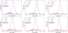 |
Fig. A.1 Distributions of counts (ADU pixel-1) over the entire masked region of empty sky for NGC 2403 and NGC 6822 (top panels); Holmberg II, IC 10 (middle); and IC 342, NGC 6744 (bottom). The data are shown as solid lines, and the Gaussian best fits as dashed ones. The four bands are given by purple, blue, green, and red for IE, YE, JE, and HE, respectively. The IE VIS band counts have been multiplied by the ratio of the pixel area (×9) to be shown together with the NIR bands. In most cases, the data (traced by a solid curve) are so close to a Gaussian as to be indistinguishable from the best fit (shown by a dashed curve). |
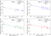 |
Fig. A.2 SB limits obtained with the various methodologies plotted against sky brightness for the four Euclid bands. For the method that does not directly give sky brightness [Approach (1)], we used the mean of the sky values from Approaches (2) and (3). There is a correlation of the SB limits with sky brightness, with brighter sky having brighter limits, and a variation with methodology, up to 0.3-0.4mag arcsec-2. |
Appendix B Euclid imaging capabilities
The continuation of Figs. 1-3 (Sect. 4) is shown here for IC 10, NGC 2403, and NGC 6822.
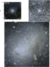 |
Fig. B.1 Same as for Fig. 1, but for IC 10, and, as before, with HE green, YE red, and IE blue. Extinction has been corrected and sky subtracted as described in the text (Sects. 3.2 and 4.1). In the top left panel, the full FoV of 0.7 × 0.7 is shown, while in the lower one the inner 6’ × 6 ‘ region is displayed corresponding to the white box in the upper left panel. The top right panel shows the zoomed-in 30ʺ × 30ʺ RGB image of the blue nucleus also seen in the radial color profiles (Sect. 4.4, App. C, and Fig. C.1); the white box in the lower panel corresponds to the zoom-in cut-out shown in the upper right. The dark boxes in IC 10 result from an incorrect orientation of the instruments relative to the roll angle of the satellite during observation (this was the first galaxy observed within the ERO Showcase). |
Appendix C Surface brightness profiles of four Showcase galaxies
Here we show surface-brightness profiles of the remaining four galaxies that are not given in the main text (Sect. 4.4).
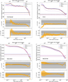 |
Fig. C.1 Surface brightness and color profiles extracted by AutoProf, as described in the text: Holmberg II and IC 10 in the top row; and NGC 2403 and NGC 6744 in the bottom. The four bands are given by purple, blue, green, and red for IE, YE, JE, and HE, respectively. The 1σ SB limits from AutoProf in units of mag arcsec-2 are shown as dashed horizontal lines, with colors corresponding to the Euclid bands. The fluxes have been corrected for foreground extinction (Sect. 4.1) in order to be consistent with the IE - HE radial color gradient shown in the middle panel, and YE - HE shown at the bottom. The uncorrected IE profile is shown as a dotted (purple) curve in the top panel. The mean IE - HE color over typically a factor of 100 in radius in the inner galaxy is shown as a horizontal dashed line in the middle panel. |
Appendix D Star-count maps of two Showcase galaxies
Here we present the maps of the star counts of the remaining two galaxies that are not shown in the main text (Sect. 5).
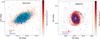 |
Fig. D.1 Star-count maps obtained as described in Sect. 5, but for NGC 2403 (left panel), and the most distant Showcase galaxy, NGC 6744 (right). |
References
- Abdurro’uf, Lin, Y.-T., Hirashita, H., et al. 2022, ApJ, 926, 81 [Google Scholar]
- Akhlaghi, M. 2019a, arXiv e-prints [arXiv:1909.11230] [Google Scholar]
- Akhlaghi, M. 2019b, in ASP Conf. Ser., 521, 299 [Google Scholar]
- Akhlaghi, M., & Ichikawa, T. 2015, ApJS, 220, 1 [Google Scholar]
- Annibali, F., & Tosi, M. 2022, Nat. Astron., 6, 48 [NASA ADS] [CrossRef] [Google Scholar]
- Arnouts, S., Cristiani, S., Moscardini, L., et al. 1999, MNRAS, 310, 540 [Google Scholar]
- Ashley, T., Elmegreen, B. G., Johnson, M., et al. 2014, AJ, 148, 130 [NASA ADS] [CrossRef] [Google Scholar]
- Astropy Collaboration (Robitaille, T. P., et al.) 2013, A&A, 558, A33 [NASA ADS] [CrossRef] [EDP Sciences] [Google Scholar]
- Astropy Collaboration (Price-Whelan, A. M., et al.) 2018, AJ, 156, 123 [Google Scholar]
- Astropy Collaboration (Price-Whelan, A. M., et al.) 2022, ApJ, 935, 167 [NASA ADS] [CrossRef] [Google Scholar]
- Barker, M. K., Ferguson, A. M. N., Irwin, M. J., Arimoto, N., & Jablonka, P. 2012, MNRAS, 419, 1489 [CrossRef] [Google Scholar]
- Balser, D. S., Wenger, T. V., Goss, W. M., Johnson, K. E., & Kepley, A. A. 2017, ApJ, 844, 73 [Google Scholar]
- Barra, F., Pinto, C., Middleton, M., et al. 2024, A&A, 682, A94 [NASA ADS] [CrossRef] [EDP Sciences] [Google Scholar]
- Battistini, P., Bonoli, F., Federici, L., Fusi Pecci, F., & Kron, R. G. 1984, A&A, 130, 162 [NASA ADS] [Google Scholar]
- Bedin, L. R., Salaris, M., Rich, R. M., et al. 2019, MNRAS, 484, L54 [NASA ADS] [Google Scholar]
- Bell, C. P. M., Cioni, M.-R. L., Wright, A. H., et al. 2019, MNRAS, 489, 3200 [Google Scholar]
- Belland, B., Kirby, E., Boylan-Kolchin, M., & Wheeler, C. 2020, ApJ, 903, 10 [NASA ADS] [CrossRef] [Google Scholar]
- Bellazzini, M., & Pascale, R. 2024, A&A, 691, A42 [NASA ADS] [CrossRef] [EDP Sciences] [Google Scholar]
- Belokurov, V., Zucker, D. B., Evans, N. W., et al. 2006, ApJ, 642, L137 [Google Scholar]
- Bennet, P., Patel, E., Sohn, S. T., et al. 2024, ApJ, 971, 98 [Google Scholar]
- Bentley, J., Tinney, C. G., Sharma, S., & Wright, D. 2019, MNRAS, 490, 4107 [Google Scholar]
- Bernard, E. J., Ferguson, A. M. N., Barker, M. K., et al. 2012, MNRAS, 426, 3490 [Google Scholar]
- Bertin, E., & Arnouts, S. 1996, A&AS, 117, 393 [NASA ADS] [CrossRef] [EDP Sciences] [Google Scholar]
- Bianchi, S., Giovanardi, C., Smith, M. W. L., et al. 2017, A&A, 597, A130 [NASA ADS] [CrossRef] [EDP Sciences] [Google Scholar]
- Blakeslee, J. P., Tonry, J. L., & Metzger, M. R. 1997, AJ, 114, 482 [Google Scholar]
- Blakeslee, J. P., Jordán, A., Mei, S., et al. 2009, ApJ, 694, 556 [Google Scholar]
- Bland-Hawthorn, J., Maloney, P. R., Stephens, A., Zovaro, A., & Popping, A. 2017, ApJ, 849, 51 [Google Scholar]
- Böker, T., van der Marel, R. P., & Vacca, W. D. 1999, AJ, 118, 831 [CrossRef] [Google Scholar]
- Boquien, M., Burgarella, D., Roehlly, Y., et al. 2019, A&A, 622, A103 [NASA ADS] [CrossRef] [EDP Sciences] [Google Scholar]
- Borlaff, A., Trujillo, I., Román, J., et al. 2019, A&A, 621, A133 [NASA ADS] [CrossRef] [EDP Sciences] [Google Scholar]
- Boselli, A., Voyer, E., Boissier, S., et al. 2014, A&A, 570, A69 [NASA ADS] [CrossRef] [EDP Sciences] [Google Scholar]
- Bosma, A. 2017, Astrophys. Space Sci. Lib., 434, 209 [Google Scholar]
- Bressan, A., Marigo, P., Girardi, L., et al. 2012, MNRAS, 427, 127 [NASA ADS] [CrossRef] [Google Scholar]
- Brodie, J. P., & Strader, J. 2006, ARA&A, 44, 193 [Google Scholar]
- Bruzual, G., & Charlot, S. 2003, MNRAS, 344, 1000 [NASA ADS] [CrossRef] [Google Scholar]
- Bullock, J. S., & Johnston, K. V. 2005, ApJ, 635, 931 [Google Scholar]
- Buta, R. J., & McCall, M. L. 1999, ApJS, 124, 33 [NASA ADS] [CrossRef] [Google Scholar]
- Calzetti, D., Kinney, A. L., & Storchi-Bergmann, T. 1994, ApJ, 429, 582 [Google Scholar]
- Cannon, J. M., O’Leary, E. M., Weisz, D. R., et al. 2012, ApJ, 747, 122 [Google Scholar]
- Cantiello, M., Grado, A., Rejkuba, M., et al. 2018a, A&A, 611, A21 [NASA ADS] [CrossRef] [EDP Sciences] [Google Scholar]
- Cantiello, M., Blakeslee, J. P., Ferrarese, L., et al. 2018b, ApJ, 856, 126 [Google Scholar]
- Carlberg, R. G., Richer, H. B., McConnachie, A. W., et al. 2011, ApJ, 731, 124 [Google Scholar]
- Carlin, J. L., Garling, C. T., Peter, A. H. G., et al. 2019, ApJ, 886, 109 [NASA ADS] [CrossRef] [Google Scholar]
- Carlsten, S. G., Beaton, R. L., Greco, J. P., & Greene, J. E. 2019, ApJ, 879, 13 [NASA ADS] [CrossRef] [Google Scholar]
- Carlsten, S. G., Greene, J. E., Beaton, R. L., & Greco, J. P. 2022, ApJ, 927, 44 [NASA ADS] [CrossRef] [Google Scholar]
- Carollo, D., Beers, T. C., Placco, V. M., et al. 2016, Nat. Phys., 12, 1170 [Google Scholar]
- Carson, D. J., Barth, A. J., Seth, A. C., et al. 2015, AJ, 149, 170 [Google Scholar]
- Chiang, I.-D., Sandstrom, K. M., Chastenet, J., et al. 2021, ApJ, 907, 29 [NASA ADS] [CrossRef] [Google Scholar]
- Choi, Y., Dalcanton, J. J., Williams, B. F., et al. 2015, ApJ, 810, 9 [Google Scholar]
- Cignoni, M., Sacchi, E., Aloisi, A., et al. 2018, ApJ, 856, 62 [NASA ADS] [CrossRef] [Google Scholar]
- Cignoni, M., Sacchi, E., Tosi, M., et al. 2019, ApJ, 887, 112 [NASA ADS] [CrossRef] [Google Scholar]
- Conselice, C. J., Mundy, C. J., Ferreira, L., & Duncan, K. 2022, ApJ, 940, 168 [CrossRef] [Google Scholar]
- Crnojevic’, D., Sand, D. J., Spekkens, K., et al. 2016, ApJ, 823, 19 [Google Scholar]
- Cseh, D., Corbel, S., Kaaret, P., et al. 2012, ApJ, 749, 17 [NASA ADS] [CrossRef] [Google Scholar]
- Cuillandre, J.-C., Bertin, E., Bolzonella, M., et al. 2025, A&A, 697, A6 (Euclid on Sky SI) [Google Scholar]
- Das, S., Nandi, A., Agrawal, V. K., Dihingia, I. K., & Majumder, S. 2021, MNRAS, 507, 2777 [Google Scholar]
- da Silva, P., Steiner, J. E., & Menezes, R. B. 2018, ApJ, 861, 83 [Google Scholar]
- Davidge, T. J. 2007, ApJ, 664, 820 [Google Scholar]
- de Blok, W. J. G., & Walter, F. 2000, ApJ, 537, L95 [NASA ADS] [CrossRef] [Google Scholar]
- de Blok, W. J. G., & Walter, F. 2003, MNRAS, 341, L39 [Google Scholar]
- de Blok, W. J. G., & Walter, F. 2006, AJ, 131, 343 [NASA ADS] [CrossRef] [Google Scholar]
- de Blok, W.J. G., Keating, K. M., Pisano, D. J., et al. 2014, A&A, 569, A68 [NASA ADS] [CrossRef] [EDP Sciences] [Google Scholar]
- de Jong, R. S., Seth, A. C., Bell, E. F., et al. 2007, in Stellar Populations as Building Blocks of Galaxies, 241, eds. A. Vazdekis, & R. Peletier, 503 [Google Scholar]
- Dell’Agli, F., Di Criscienzo, M., Ventura, P., et al. 2018, MNRAS, 479, 5035 [Google Scholar]
- Demers, S., Battinelli, P., & Kunkel, W. E. 2006, ApJ, 636, L85 [NASA ADS] [CrossRef] [Google Scholar]
- de Vaucouleurs, G. 1963, ApJ, 138, 934 [NASA ADS] [CrossRef] [Google Scholar]
- Egorov, O. V., Lozinskaya, T. A., Moiseev, A. V., & Shchekinov, Y. A. 2017, MNRAS, 464, 1833 [NASA ADS] [CrossRef] [Google Scholar]
- Euclid Collaboration (Borlaff, A. S., et al.) 2022, A&A, 657, A92 [NASA ADS] [CrossRef] [EDP Sciences] [Google Scholar]
- Euclid Collaboration (Scaramella, R., et al.) 2022, A&A, 662, A112 [NASA ADS] [CrossRef] [EDP Sciences] [Google Scholar]
- Euclid Collaboration (Schirmer, M., et al.) 2022, A&A, 662, A92 [NASA ADS] [CrossRef] [EDP Sciences] [Google Scholar]
- Euclid Collaboration (Cropper, M. S., et al.) 2025, A&A, 697, A2 (Euclid on Sky SI) [Google Scholar]
- Euclid Collaboration (Jahnke, K., et al.) 2025, A&A, 697, A3 (Euclid on Sky SI) [Google Scholar]
- Euclid Collaboration (Mellier, Y., et al.) 2025, A&A, 697, A1 (Euclid on Sky SI) [Google Scholar]
- Euclid Collaboration (Voggel, K., et al.) 2025, A&A, 693, A251 [Google Scholar]
- Euclid Early Release Observations 2024, https://doi.org/10.57780/esa-qmocze3 [Google Scholar]
- Ferguson, A. M. N., Irwin, M. J., Ibata, R. A., Lewis, G. F., & Tanvir, N. R. 2002, AJ, 124, 1452 [Google Scholar]
- Fioc, M. & Rocca-Volmerange, B. 1997, A&A, 326, 950 [Google Scholar]
- Forbes, D. A., & Bridges, T. 2010, MNRAS, 404, 1203 [NASA ADS] [Google Scholar]
- Forbes, D. A., Franx, M., Illingworth, G. D., & Carollo, C. M. 1996, ApJ, 467, 126 [Google Scholar]
- Forbes, D. A., Ferré-Mateu, A., Gannon, J. S., et al. 2022, MNRAS, 512, 802 [NASA ADS] [CrossRef] [Google Scholar]
- Fraternali, F., & Binney, J. J. 2008, MNRAS, 386, 935 [CrossRef] [Google Scholar]
- Fraternali, F., van Moorsel, G., Sancisi, R., & Oosterloo, T. 2002, AJ, 123, 3124 [CrossRef] [Google Scholar]
- Fusco, F., Buonanno, R., Bono, G., et al. 2012, A&A, 548, A129 [NASA ADS] [CrossRef] [EDP Sciences] [Google Scholar]
- Gaia Collaboration (Brown, A. G. A., et al.) 2021, A&A, 649, A1 [NASA ADS] [CrossRef] [EDP Sciences] [Google Scholar]
- Gerbrandt, S. A. N., McConnachie, A. W., & Irwin, M. 2015, MNRAS, 454, 1000 [NASA ADS] [CrossRef] [Google Scholar]
- Gerola, H., & Seiden, P. E. 1978, ApJ, 223, 129 [Google Scholar]
- Girardi, L., Groenewegen, M. A. T., Hatziminaoglou, E., & da Costa, L. 2005, A&A, 436, 895 [NASA ADS] [CrossRef] [EDP Sciences] [Google Scholar]
- Girardi, L., Barbieri, M., Groenewegen, M. A. T., et al. 2012, in Astrophysics and Space Science Proceedings, 26, Red Giants as Probes of the Structure and Evolution of the Milky Way, 165 [Google Scholar]
- Goad, M. R., Roberts, T. P., Reeves, J. N., & Uttley, P. 2006, MNRAS, 365, 191 [NASA ADS] [CrossRef] [Google Scholar]
- Gogarten, S. M., Dalcanton, J. J., Williams, B. F., et al. 2010, ApJ, 712, 858 [NASA ADS] [CrossRef] [Google Scholar]
- Gordon, K. D., Clayton, G. C., Misselt, K. A., Landolt, A. U., & Wolff, M. J. 2003, ApJ, 594, 279 [NASA ADS] [CrossRef] [Google Scholar]
- Gordon, K. D., Clayton, G. C., Decleir, M., et al. 2023, ApJ, 950, 86 [CrossRef] [Google Scholar]
- Hammer, F., Flores, H., Elbaz, D., et al. 2005, A&A, 430, 115 [NASA ADS] [CrossRef] [EDP Sciences] [Google Scholar]
- Harris, W. E. 1996, AJ, 112, 1487 [Google Scholar]
- Harris, W. E. 2009, ApJ, 699, 254 [NASA ADS] [CrossRef] [Google Scholar]
- Harris, W. E., & Racine, R. 1979, ARA&A, 17, 241 [NASA ADS] [CrossRef] [Google Scholar]
- Harris, W. E., Harris, G. L. H., & Alessi, M. 2013, ApJ, 772, 82 [Google Scholar]
- Heesen, V., Brinks, E., Krause, M. G. H., et al. 2015, MNRAS, 447, L1 [NASA ADS] [CrossRef] [Google Scholar]
- Heesen, V., Rafferty, D. A., Horneffer, A., et al. 2018, MNRAS, 476, 1756 [NASA ADS] [CrossRef] [Google Scholar]
- Helmi, A., Babusiaux, C., Koppelman, H. H., et al. 2018, Nature, 563, 85 [Google Scholar]
- Hillis, T. J., Williams, B. F., Dolphin, A. E., Dalcanton, J. J., & Skillman, E. D. 2016, ApJ, 831, 191 [Google Scholar]
- Hodge, P., & Lee, M. G. 1990, PASP, 102, 26 [Google Scholar]
- Hodge, P., Strobel, N. V., & Kennicutt, R. C. 1994, PASP, 106, 309 [Google Scholar]
- Holmberg, E. 1950, Meddel. fran Lunds Astron. Observ. Ser. II, 128, 5 [Google Scholar]
- Hubble, E. P. 1925, ApJ, 62, 409 [NASA ADS] [CrossRef] [Google Scholar]
- Hunter, D. A. 2001, ApJ, 559, 225 [Google Scholar]
- Huxor, A. P., Ferguson, A. M. N., Veljanoski, J., Mackey, A. D., & Tanvir, N. R. 2013, MNRAS, 429, 1039 [NASA ADS] [CrossRef] [Google Scholar]
- Ibata, R., Lewis, G. F., Irwin, M., Totten, E., & Quinn, T. 2001, ApJ, 551, 294 [Google Scholar]
- Ibata, R., Martin, N. F., Irwin, M., et al. 2007, ApJ, 671, 1591 [CrossRef] [Google Scholar]
- Ilbert, O., Arnouts, S., McCracken, H. J., et al. 2006, A&A, 457, 841 [NASA ADS] [CrossRef] [EDP Sciences] [Google Scholar]
- Jang, I. S., de Jong, R. S., Holwerda, B. W., et al. 2020a, A&A, 637, A8 [NASA ADS] [CrossRef] [EDP Sciences] [Google Scholar]
- Jang, I. S., de Jong, R. S., Minchev, I., et al. 2020b, A&A, 640, L19 [NASA ADS] [CrossRef] [EDP Sciences] [Google Scholar]
- Jarrett, T. H., Cluver, M. E., Brown, M. J. I., et al. 2019, ApJS, 245, 25 [Google Scholar]
- Johnston, K. V., Sackett, P. D., & Bullock, J. S. 2001, ApJ, 557, 137 [NASA ADS] [CrossRef] [Google Scholar]
- Juric’, M., Ivezic’, Ž., Brooks, A., et al. 2008, ApJ, 673, 864 [NASA ADS] [CrossRef] [Google Scholar]
- Kaaret, P., Ward, M. J., & Zezas, A. 2004, MNRAS, 351, L83 [NASA ADS] [CrossRef] [Google Scholar]
- Kamphuis, J., & Briggs, F. 1992, A&A, 253, 335 [NASA ADS] [Google Scholar]
- Kankare, E., Fraser, M., Ryder, S., et al. 2014, A&A, 572, A75 [EDP Sciences] [Google Scholar]
- Karachentsev, I. D., Dolphin, A. E., Geisler, D., et al. 2002, A&A, 383, 125 [CrossRef] [EDP Sciences] [Google Scholar]
- Karachentsev, I. D., Kaisina, E. I., & Makarov, D. I. 2014, AJ, 147, 13 [Google Scholar]
- Karachentsev, I. D., Riepe, P., & Zilch, T. 2020, Astrophysics, 63, 5 [Google Scholar]
- Kennicutt, R. C., Calzetti, D., Aniano, G., et al. 2011, PASP, 123, 1347 [Google Scholar]
- King, I. 1962, AJ, 67, 471 [Google Scholar]
- Kluge, M., Hatch, N. A., Montes, M., et al. 2025, A&A, 697, A13 (Euclid on Sky SI) [NASA ADS] [CrossRef] [EDP Sciences] [Google Scholar]
- Komiyama, Y., Okamura, S., Yagi, M., et al. 2003, ApJ, 590, L17 [Google Scholar]
- Komiyama, Y., Chiba, M., Tanaka, M., et al. 2018, ApJ, 853, 29 [NASA ADS] [CrossRef] [Google Scholar]
- Kruijssen, J. M. D. 2015, MNRAS, 454, 1658 [Google Scholar]
- Larsen, S. S. 1999, A&AS, 139, 393 [NASA ADS] [CrossRef] [EDP Sciences] [Google Scholar]
- Larsen, S., & Richtler, T. 1998, ASP Conf. Ser., 136, 67 [Google Scholar]
- Larsen, S. S., Brodie, J. P., Huchra, J. P., Forbes, D. A., & Grillmair, C. J. 2001, AJ, 121, 2974 [NASA ADS] [CrossRef] [Google Scholar]
- Larsen, S. S., Brodie, J. P., Wasserman, A., & Strader, J. 2018, A&A, 613, A56 [NASA ADS] [CrossRef] [EDP Sciences] [Google Scholar]
- Larsen, S. S., Eitner, P., Magg, E., et al. 2022, A&A, 660, A88 [NASA ADS] [CrossRef] [EDP Sciences] [Google Scholar]
- Laureijs, R., Amiaux, J., Arduini, S., et al. 2011, arXiv e-prints [arXiv:1110.3193] [Google Scholar]
- Lazzarini, M., Williams, B. F., Durbin, M. J., et al. 2022, ApJ, 934, 76 [Google Scholar]
- Le Borgne, D., Rocca-Volmerange, B., Prugniel, P., et al. 2004, A&A, 425, 881 [CrossRef] [EDP Sciences] [Google Scholar]
- Lee, H., Skillman, E. D., & Venn, K. A. 2006, ApJ, 642, 813 [Google Scholar]
- Lelli, F., Verheijen, M., & Fraternali, F. 2014, MNRAS, 445, 1694 [Google Scholar]
- Leroy, A. K., Schinnerer, E., Hughes, A., et al. 2021, ApJS, 257, 43 [NASA ADS] [CrossRef] [Google Scholar]
- Lewis, G. F., Braun, R., McConnachie, A. W., et al. 2013, ApJ, 763, 4 [NASA ADS] [CrossRef] [Google Scholar]
- Li, A., Fraternali, F., Marasco, A., et al. 2023, MNRAS, 520, 147 [NASA ADS] [CrossRef] [Google Scholar]
- Lim, S., & Lee, M. G. 2015, ApJ, 804, 123 [NASA ADS] [CrossRef] [Google Scholar]
- Mackey, A. D., Ferguson, A. M. N., Huxor, A. P., et al. 2019, MNRAS, 484, 1756 [NASA ADS] [CrossRef] [Google Scholar]
- Madden, S. C., Rémy-Ruyer, A., Galametz, M., et al. 2013, PASP, 125, 600 [NASA ADS] [CrossRef] [Google Scholar]
- Majewski, S. R., Skrutskie, M. F., Weinberg, M. D., & Ostheimer, J. C. 2003, ApJ, 599, 1082 [NASA ADS] [CrossRef] [Google Scholar]
- Mak, D. S. Y., Pun, C. S. J., & Kong, A. K. H. 2008, ApJ, 686, 995 [Google Scholar]
- Mancera Piña, P. E., Fraternali, F., Oosterloo, T., et al. 2022, MNRAS, 514, 3329 [CrossRef] [Google Scholar]
- Marigo, P., Girardi, L., Bressan, A., et al. 2017, ApJ, 835, 77 [Google Scholar]
- Marleau, F. R., Habas, R., Poulain, M., et al. 2021, A&A, 654, A105 [NASA ADS] [CrossRef] [EDP Sciences] [Google Scholar]
- Martin, G., Bazkiaei, A. E., Spavone, M., et al. 2022a, MNRAS, 513, 1459 [Google Scholar]
- Martin, N. F., Ibata, R. A., Starkenburg, E., et al. 2022b, MNRAS, 516, 5331 [Google Scholar]
- Martínez-Delgado, D., Peñarrubia, J., Gabany, R. J., et al. 2008, ApJ, 689, 184 [CrossRef] [Google Scholar]
- Martínez-Delgado, D., Pohlen, M., Gabany, R. J., et al. 2009, ApJ, 692, 955 [CrossRef] [Google Scholar]
- Martínez-Delgado, D., Gabany, R. J., Crawford, K., et al. 2010, AJ, 140, 962 [Google Scholar]
- Martínez-Delgado, D., Cooper, A. P., Román, J., et al. 2023, A&A, 671, A141 [NASA ADS] [CrossRef] [EDP Sciences] [Google Scholar]
- Massey, P., Olsen, K. A. G., Hodge, P. W., et al. 2007, AJ, 133, 2393 [Google Scholar]
- Mayer, L., Mastropietro, C., Wadsley, J., Stadel, J., & Moore, B. 2006, MNRAS, 369, 1021 [NASA ADS] [CrossRef] [Google Scholar]
- McConnachie, A. W., Irwin, M. J., Ibata, R. A., et al. 2009, Nature, 461, 66 [Google Scholar]
- McConnachie, A. W., Ferguson, A. M. N., Irwin, M. J., et al. 2010, ApJ, 723, 1038 [NASA ADS] [CrossRef] [Google Scholar]
- McConnachie, A. W., Higgs, C. R., Thomas, G. F., et al. 2021, MNRAS, 501, 2363 [NASA ADS] [CrossRef] [Google Scholar]
- McQuinn, K. B. W., Skillman, E. D., Cannon, J. M., et al. 2010, ApJ, 721, 297 [NASA ADS] [CrossRef] [Google Scholar]
- Mei, S., Blakeslee, J. P., Tonry, J. L., et al. 2005, ApJ, 625, 121 [Google Scholar]
- Mei, S., Blakeslee, J. P., Côté, P., et al. 2007, ApJ, 655, 144 [Google Scholar]
- Merritt, A., van Dokkum, P., Abraham, R., & Zhang, J. 2016, ApJ, 830, 62 [Google Scholar]
- Mihos, J. C. 2019, arXiv e-prints [arXiv:1909.09456] [Google Scholar]
- Mihos, J. C., & Hernquist, L. 1994, ApJ, 425, L13 [Google Scholar]
- Mihos, J. C., Durrell, P. R., Ferrarese, L., et al. 2015, ApJ, 809, L21 [Google Scholar]
- Muñoz, R. P., Eigenthaler, P., Puzia, T. H., et al. 2015, ApJ, 813, L15 [Google Scholar]
- Mundy, C. J., Conselice, C. J., Duncan, K. J., et al. 2017, MNRAS, 470, 3507 [Google Scholar]
- Nally, C., Jones, O. C., Lenkic’, L., et al. 2024, MNRAS, 531, 183 [NASA ADS] [CrossRef] [Google Scholar]
- Namumba, B., Carignan, C., Foster, T., & Deg, N. 2019, MNRAS, 490, 3365 [Google Scholar]
- Nersesian, A., Xilouris, E. M., Bianchi, S., et al. 2019, A&A, 624, A80 [NASA ADS] [CrossRef] [EDP Sciences] [Google Scholar]
- Nidever, D. L., Ashley, T., Slater, C. T., et al. 2013, ApJ, 779, L15 [NASA ADS] [CrossRef] [Google Scholar]
- Okamoto, S., Arimoto, N., Ferguson, A. M. N., et al. 2015, ApJ, 809, L1 [NASA ADS] [CrossRef] [Google Scholar]
- Pancino, E., Romano, D., Tang, B., et al. 2017, A&A, 601, A112 [NASA ADS] [CrossRef] [EDP Sciences] [Google Scholar]
- Patrick, L. R., Evans, C. J., Davies, B., et al. 2015, ApJ, 803, 14 [Google Scholar]
- Peng, E. W., Jordán, A., Blakeslee, J. P., et al. 2009, ApJ, 703, 42 [NASA ADS] [CrossRef] [Google Scholar]
- Peters, S. P. C., van der Kruit, P. C., Knapen, J. H., et al. 2017, MNRAS, 470, 427 [NASA ADS] [CrossRef] [Google Scholar]
- Pilyugin, L. S., Grebel, E. K., & Kniazev, A. Y. 2014, AJ, 147, 131 [NASA ADS] [CrossRef] [Google Scholar]
- Planck Collaboration XXIV. 2011, A&A, 536, A24 [NASA ADS] [CrossRef] [EDP Sciences] [Google Scholar]
- Polles, F. L., Madden, S. C., Lebouteiller, V., et al. 2019, A&A, 622, A119 [NASA ADS] [CrossRef] [EDP Sciences] [Google Scholar]
- Pota, V., Forbes, D. A., Romanowsky, A. J., et al. 2013, MNRAS, 428, 389 [NASA ADS] [CrossRef] [Google Scholar]
- Puche, D., Westpfahl, D., Brinks, E., & Roy, J.-R. 1992, AJ, 103, 1841 [Google Scholar]
- Radburn-Smith, D. J., de Jong, R. S., Seth, A. C., et al. 2011, ApJS, 195, 18 [Google Scholar]
- Rejkuba, M. 2012, Ap&SS, 341, 195 [Google Scholar]
- Reynolds, T. N., Catinella, B., Cortese, L., et al. 2022, MNRAS, 510, 1716 [Google Scholar]
- Reynolds, T. N., Catinella, B., Cortese, L., et al. 2023, PASA, 40, e032 [Google Scholar]
- Rhode, K. L., Salzer, J. J., Westpfahl, D. J., & Radice, L. A. 1999, AJ, 118, 323 [Google Scholar]
- Roberts, W. W. J., & Hausman, M. A. 1984, ApJ, 277, 744 [Google Scholar]
- Roberts, T. P., Goad, M. R., Ward, M. J., & Warwick, R. S. 2003, MNRAS, 342, 709 [NASA ADS] [CrossRef] [Google Scholar]
- Ryder, S. D., Walsh, W., & Malin, D. 1999, PASA, 16, 84 [NASA ADS] [CrossRef] [Google Scholar]
- Román, J., Trujillo, I., & Montes, M. 2020, A&A, 644, A42 [NASA ADS] [CrossRef] [EDP Sciences] [Google Scholar]
- Román, J., Castilla, A., & Pascual-Granado, J. 2021, A&A, 656, A44 [NASA ADS] [CrossRef] [EDP Sciences] [Google Scholar]
- Román, J., Sánchez-Alarcón, P. M., Knapen, J. H., & Peletier, R. 2023a, A&A, 671, L7 [NASA ADS] [CrossRef] [EDP Sciences] [Google Scholar]
- Román, J., Rich, R. M., Ahvazi, N., et al. 2023b, A&A, 679, A157 [NASA ADS] [CrossRef] [EDP Sciences] [Google Scholar]
- Sabbi, E., Calzetti, D., Ubeda, L., et al. 2018, ApJS, 235, 23 [Google Scholar]
- Saifollahi, T., Voggel, K., Lançon, A., et al. 2025, A&A, 697, A10 (Euclid on Sky SI) [NASA ADS] [CrossRef] [EDP Sciences] [Google Scholar]
- Sánchez, S. F., Rosales-Ortega, F. F., Iglesias-Páramo, J., et al. 2014, A&A, 563, A49 [CrossRef] [EDP Sciences] [Google Scholar]
- Sánchez-Alarcón, P. M., Román, J., Knapen, J. H., et al. 2023, A&A, 677, A117 [NASA ADS] [CrossRef] [EDP Sciences] [Google Scholar]
- Schlafly, E. F., & Finkbeiner, D. P. 2011, ApJ, 737, 103 [Google Scholar]
- Schlegel, D. J., Finkbeiner, D. P., & Davis, M. 1998, ApJ, 500, 525 [Google Scholar]
- Shostak, G. S., & Skillman, E. D. 1989, A&A, 214, 33 [NASA ADS] [Google Scholar]
- Sibbons, L. F., Ryan, S. G., Cioni, M. R. L., Irwin, M., & Napiwotzki, R. 2012, A&A, 540, A135 [NASA ADS] [CrossRef] [EDP Sciences] [Google Scholar]
- Silverman, J. M., & Filippenko, A. V. 2008, ApJ, 678, L17 [NASA ADS] [CrossRef] [Google Scholar]
- Sola, E., Duc, P.-A., Richards, F., et al. 2022, A&A, 662, A124 [NASA ADS] [CrossRef] [EDP Sciences] [Google Scholar]
- Stetson, P. B. 1987, PASP, 99, 191 [Google Scholar]
- Stetson, P. B. 1994, PASP, 106, 250 [Google Scholar]
- Stewart, S. G., Fanelli, M. N., Byrd, G. G., et al. 2000, ApJ, 529, 201 [NASA ADS] [CrossRef] [Google Scholar]
- Stone, C. J., Arora, N., Courteau, S., & Cuillandre, J.-C. 2021, MNRAS, 508, 1870 [NASA ADS] [CrossRef] [Google Scholar]
- Tammann, G. A., & Sandage, A. 1968, ApJ, 151, 825 [NASA ADS] [CrossRef] [Google Scholar]
- Tantalo, M., Dall’Ora, M., Bono, G., et al. 2022, ApJ, 933, 197 [NASA ADS] [CrossRef] [Google Scholar]
- Teyssier, M., Johnston, K. V., & Kuhlen, M. 2012, MNRAS, 426, 1808 [NASA ADS] [CrossRef] [Google Scholar]
- Thompson, G. P., Ryan, S. G., & Sibbons, L. F. 2016, MNRAS, 462, 3376 [Google Scholar]
- Tonry, J. L., Dressler, A., Blakeslee, J. P., et al. 2001, ApJ, 546, 681 [Google Scholar]
- Tran, D., Williams, B., Levesque, E., et al. 2023, ApJ, 954, 211 [NASA ADS] [CrossRef] [Google Scholar]
- Trujillo, I., & Fliri, J. 2016, ApJ, 823, 123 [Google Scholar]
- Vacca, W. D., Sheehy, C. D., & Graham, J. R. 2007, ApJ, 662, 272 [Google Scholar]
- van den Bergh, S. 1999, A&A Rev., 9, 273 [Google Scholar]
- van der Kruit, P. C. 1981, A&A, 99, 298 [NASA ADS] [Google Scholar]
- van Dokkum, P. G., Abraham, R., Merritt, A., et al. 2015, ApJ, 798, L45 [NASA ADS] [CrossRef] [Google Scholar]
- Veljanoski, J., Ferguson, A. M. N., Mackey, A. D., et al. 2015, MNRAS, 452, 320 [NASA ADS] [CrossRef] [Google Scholar]
- Venhola, A., Peletier, R. F., Salo, H., et al. 2022, A&A, 662, A43 [NASA ADS] [CrossRef] [EDP Sciences] [Google Scholar]
- Venn, K. A., Lennon, D. J., Kaufer, A., et al. 2001, ApJ, 547, 765 [NASA ADS] [CrossRef] [Google Scholar]
- Veronese, S., de Blok, W. J. G., & Walter, F. 2023, A&A, 672, A55 [NASA ADS] [CrossRef] [EDP Sciences] [Google Scholar]
- Wada, K., Baba, J., & Saitoh, T. R. 2011, ApJ, 735, 1 [NASA ADS] [CrossRef] [Google Scholar]
- Walter, F., Brinks, E., de Blok, W. J. G., et al. 2008, AJ, 136, 2563 [Google Scholar]
- Wang, J., Kauffmann, G., Overzier, R., et al. 2011, MNRAS, 412, 1081 [Google Scholar]
- Weisz, D. R., Skillman, E. D., Cannon, J. M., et al. 2009, ApJ, 704, 1538 [NASA ADS] [CrossRef] [Google Scholar]
- Weisz, D. R., Dalcanton, J. J., Williams, B. F., et al. 2011, ApJ, 739, 5 [CrossRef] [Google Scholar]
- Weisz, D. R., Dolphin, A. E., Skillman, E. D., et al. 2014, ApJ, 789, 147 [Google Scholar]
- Wilcots, E. M., & Miller, B. W. 1998, AJ, 116, 2363 [Google Scholar]
- Williams, B. F., Dalcanton, J. J., Seth, A. C., et al. 2009a, AJ, 137, 419 [Google Scholar]
- Williams, B. F., Dalcanton, J. J., Dolphin, A. E., Holtzman, J., & Sarajedini, A. 2009b, ApJ, 695, L15 [Google Scholar]
- Williams, B. F., Dalcanton, J. J., Stilp, A., et al. 2013, ApJ, 765, 120 [NASA ADS] [CrossRef] [Google Scholar]
- Wu, P.-F., Tully, R. B., Rizzi, L., et al. 2014, AJ, 148, 7 [NASA ADS] [CrossRef] [Google Scholar]
- Xu, C. K., Cheng, C., Appleton, P. N., et al. 2022, Nature, 610, 461 [NASA ADS] [CrossRef] [Google Scholar]
- Yew, M., Filipovic’, M. D., Roper, Q., et al. 2018, PASA, 35, e015 [Google Scholar]
- Žemaitis, R., Ferguson, A. M. N., Okamoto, S., et al. 2023, MNRAS, 518, 2497 [Google Scholar]
- Zezas, A. L., Georgantopoulos, I., & Ward, M. J. 1999, MNRAS, 308, 302 [Google Scholar]
- Zhang, S., Mackey, D., & Da Costa, G. S. 2021, MNRAS, 508, 2098 [NASA ADS] [CrossRef] [Google Scholar]
dustmaps is found at https://dustmaps.readthedocs.io/en/latest/maps.html and the dust maps themselves can be accessed and downloaded in the context of this package.
Available at https://dust-extinction.readthedocs.io/en/stable/
The PARSEC isochrones in the Euclid bands were downloaded from http://stev.oapd.inaf.it/cgi-bin/cmd
There are notable discrepancies for many of their candidates between the coordinates listed by Battistini et al. (1984) and the locations given on their finding chart.
All Tables
Sky levels and SB limiting magnitudes μlim within 100 arcsec2 areas in empty sky regions
All Figures
|
Fig. 1 RGB image of Holmberg II with HE red, YE green, and IE blue. Foreground extinction has been corrected and sky subtracted as described in the text (Sect. 4.1). In the top panel, the full FoV of 0.7 × 0.7 is shown, while the bottom panel displays the inner 6’ × 6 ’ region corresponding to the white box in the upper panel. In the lower panel, to the east, there is an extensive north-south chain of H II regions (e.g., Hodge et al. 1994) that harbors the ultraluminous X-ray source Ho II ULX-1 (e.g., Zezas et al. 1999; Kaaret et al. 2004), visible as a triangular-shaped blue H II region at α = 08:19:28.98, δ = +70:42:19.3 (J2000). Also visible as a blue circular structure to the north of the H II-region chain is an artifact dichroic ghost (see also Sect. 6, Fig. 15). |
| In the text | |
|
Fig. 2 As in Fig. 1, but for IC 342, and with the top left panel showing the full FoV of 0.7 × 0.7 and the bottom panel showing the inner 6’ × 6’ region corresponding to the white box in the upper left. The top right panel shows the zoomed-in 30ʺ × 30ʺ RGB image of the blue nucleus, also revealed in the radial color profiles (see Sect. 4.4, Fig. 6). |
| In the text | |
|
Fig. 3 As in Fig. 1, but for NGC 6744, the most distant galaxy of the Showcase. In the top panel, the full FoV of 0.7 × 0.7 is shown, while the lower panel gives the inner 6’ × 6 ‘ region corresponding to the white box in the upper panel. The filamentary dust lanes within the spiral arms are delineated with exquisite detail. |
| In the text | |
|
Fig. 4 HI overlays on high-contrast Euclid IE images: IC 10 (top panel); and IC 342 (middle). The H I beam size is shown in the lower left corner, and contours are at 2σ, 4σ, 7σ, 10σ, and 20σ. The bottom panel gives the H I overlay for IC 10 as in the top panel, but using the 3-arcmin beam-smoothed H I image from Namumba et al. (2019); contours are at 2σ, 3σ, 5σ, 10σ, 10σ, and 70σ. |
| In the text | |
|
Fig. 5 Herschel SPIRE 250 μm overlays on high-contrast Euclid IE images for IC 10 (left panel) and IC 342 (right). |
| In the text | |
|
Fig. 6 Top: Surface brightness profiles and color profiles extracted by AutoProf as described in the text for IC 342 (left panel) and NGC 6822 (right). Upper panel: SB radial profiles for IE, YE, JE, and HE . The four bands are shown as purple, blue, green, and red curves for IE, YE, JE, and HE, respectively. The 1σ SB limits from AutoProf (not rescaled to 100 arcsec2 regions) in units of mag arcsec-2 are shown as dashed horizontal lines, with colors corresponding to the Euclid bands. The fluxes have been corrected for foreground extinction (see Sect. 4.1); the uncorrected IE profile is shown as a dotted (purple) curve in the top panel. Middle and bottom: IE - HE and YE - HE radial color profiles. The top axis corresponds to galactocentric radii in units of arcsec, and the bottom in units of kpc. The mean IE - HE color over typically a factor of 100 in radius is shown as a horizontal dashed line in the middle panel; the light gray rectangular regions illustrate the full spread in model colors (see Fig. 7) and the dark gray one the standard deviation about the mean of the models. The mean galaxy IE - HE with its standard deviation is also shown as a gray rectangular region in Fig. 7. |
| In the text | |
|
Fig. 7 Synthetic IE - HE from the Bruzual & Charlot (2003) models with exponentially declining SFH (left panel); the same Bruzual & Charlot (2003) models but SSPs (middle); and PEGASE SSP models from Fioc & Rocca-Volmerange (1997, right) and Le Borgne et al. (2004). The SSP models have no internal extinction applied to the colors. Also shown as gray regions are the mean IE - HE colors and their standard deviations, as reported in the middle panel of Figs. 6 and C.1, evaluated over a factor of 100 in galactocentric radius. As discussed in Sect. 4.1, these colors have been corrected for foreground extinction from our Galaxy. The different behavior of the models is due to the smoothed-out SFH in the left panel, and the different treatment of red supergiants that begin to dominate around 10 Myr, and the most massive AGB stars around 100 Myr. |
| In the text | |
|
Fig. 8 SourceExtractor output parameters for NGC 6822, intended to illustrate the typical selection cuts applied to our photometric catalogs. Purple points are the sources matched in all four Euclid bands, while yellow points correspond to our selections. In the top panel, we retain all sources with a measured FWHM in VIS of between 1.2 and 2.5 pixels, while in the bottom panel, we show our adopted selection in the plane defined by central surface brightness versus aperture magnitude. Sources with a FWHM smaller than 1.2 pixels (namely smaller than the PSF) are likely artifacts, while sources with large FWHM values and/or large values of μmax compared to aperture photometry are either saturated stars or extended objects (background galaxies or resolved star clusters). |
| In the text | |
|
Fig. 9 IE versus IE-HE color-magnitude diagram of all sources within the FoV of NGC 6822 after applying the selection cuts described in Sect. 5.1 and illustrated in Fig. 8 and after correction for foreground extinction (Sect. 5.2). Yellow points indicate bright MW and background galaxy contaminants, namely sources cross-matched with the Gaia DR3 catalog that have a measured proper motion PM larger than 3σPM. The vertical feature at IE - HE ≃ 1.3, IE ≳ 21 is due to the M dwarf population of the MW. |
| In the text | |
|
Fig. 10 Distribution in the YE - HE versus IE - HE plane of sources in the NGC 6822 photometric catalog after removal of bright IE ≲ 20 MW disk stars in Gaia DR3. In the top panel, the PARSEC stellar isochrones (Bressan et al. 2012; Marigo et al. 2017) in the Euclid bands are superimposed in red for different ages (from 10 Myr to 10 Gyr) and metallicities of Z ≲ 0.006 (about one-third solar); the TRILEGAL Galaxy model is shown in blue. Giant stars in NGC 6822 and dwarf stars in the MW overlap at IE - HE ≲ 1, while the two populations diverge at redder colors. In the bottom panel, we denote the location of Galactic M dwarf stars, AGB stars in NGC 6822, background compact red galaxies, and residual spurious detections. The dashed orange polygon outlines our final selection, which provides a reasonable compromise between the need to retain the largest possible number of stars belonging to NGC 6822, while removing Galactic M dwarfs, compact red galaxies, and residual spurious detections (see text for details). |
| In the text | |
|
Fig. 11 CMDs of the final calibrated reddening-corrected photometry for NGC 6822, after removal of extended background galaxies, bright MW contaminants and faint Galactic M dwarf stars. Left panel: IE versus IE - HE . The main stellar evolutionary sequences are indicated: the blue plume (BP), populated by massive MS and post-MS stars in the hot core helium-burning phase (ages ≲ 100 Myr); RSGs with ages from about 20Myr to 50 Myr; bright and red AGB stars with ages from 0.1 to 2 Gyr; red giant branch (RGB) stars, with ages older than 1-2 Gyr; the red clump (RC) of low-mass stars in the core-helium burning phase; and the AGB bump (AGBb). The blue, green, and red polygons, driven by the comparison with stellar evolutionary models, indicate the selection regions used to create the star count maps in Sect. 5.5. as indicated in the legend. Middle: IE versus IE - HE (same as left panel) with superimposed PARSEC stellar isochrones for different ages (10 Myr to 10 Gyr) and for two metallicity values, Z = 0.006 and 0.001 (40% and 6% solar, respectively.). Right: JE versus YE - HE. In this diagram, the oxygen-rich and the carbon-rich AGB stars (O-AGB and C-AGB) appear well separated and define vertical and horizontal sequences, respectively. |
| In the text | |
|
Fig. 12 Maps of star counts of two Showcase galaxies divided into individual stellar populations as described in the text: IC 10 (left panel); and IC 342 (right). Young stars are shown as blue points, AGB stars as green, and evolved RGB stars as red. More details are given in the text. In IC 10 (left panel), young stars are clearly more concentrated than the older ones, and in IC 342 (right), the young stars clearly delineate the spiral arms out to large galactocentric radii. |
| In the text | |
|
Fig. 13 Star-count maps obtained as for Fig. 12, but for the closest Showcase galaxy, NGC 6822 (left panel), and with HI contours overlaid on the maps (right). HI data are taken from de Blok & Walter (2000); contours are at 2σ, 4σ, 7σ, 10σ, and 20σ. The young stars in NGC 6822 are clearly aligned with the atomic gas, as discussed in the text. |
| In the text | |
|
Fig. 14 Star-count maps obtained as for Fig. 12, but for Holmberg II with H I contours overlaid (top panel); the bottom panel shows the zoomed-in image corresponding to the 15’ × 15’ gray box (shown in the top panel). H I data are taken from Walter et al. (2008); contours are at 2σ, 4σ, 7σ, 10σ, and 20σ. The AGB and old RGB stars are not visible in the map of Holmberg II because they are entirely covered by young stars. |
| In the text | |
|
Fig. 15 Euclid RGB images of the four previously known dwarf satellites from Carlsten et al. (2022) that fall in the field of view of the Euclid image of NGC 6744. Red is given by HE, green by YE, and blue by IE. The sizes of the images are 250ʺ, 150ʺ, 120ʺ, and 120ʺ on a side, from left to right; north is up, east to the left. With the exception of NGC 6744A, a well-known dwarf satellite lying along spiral arms to the northwest of the nucleus, name designations are from Carlsten et al. (2022). In the cut-out of dw1906m6357 (third panel from the left), there are also two blue circular structures that are dichroic ghost artifacts (see also Fig. 1). |
| In the text | |
|
Fig. 16 Confirmation image of a previously identified dwarf satellite of NGC 6744, dw1909m6341; the image on the left is 50ʺ × 50ʺ. The larger 12’ ×12’ image on the right shows its location near a dense stellar region that belongs to one of the spiral arms of the galaxy. The images are oriented with north up, and east to the left. |
| In the text | |
|
Fig. 17 Comparison of the zoomed-in images of one of the known satellites (left panel, dw1906m6357) shown in Fig. 15 and a galaxy (dw1912m6351, right panel) identified as a background object based on surface brightness fluctuation measurements by Carlsten et al. (2022). The sharp PSF of Euclid allows us to clearly see that the stellar population is resolved in the image on the left (satellite), but not in the image on the right (background galaxy). The images are 40ʺ on a side, with north up, and east to the left. |
| In the text | |
|
Fig. 18 Euclid VIS images of known GCs in NGC 2403 (top), young clusters (middle), and nonclusters (bottom). Each image shows a 5ʺ × 5ʺ cut-out around each object. North is up, and east to the left in all images. |
| In the text | |
|
Fig. 19 New GC candidates identified in the Euclid VIS images. Each stamp image shows a 5ʺ × 5ʺ cut-out around each object. North is up, and east to the left in all images. |
| In the text | |
|
Fig. 20 Color-magnitude diagram for known young and old clusters in NGC 2403 and our newly identified cluster candidates. |
| In the text | |
|
Fig. 21 Euclid VIS image of NGC 2403 with previously known GCs (magenta, see also Fig. 18), new GC candidates (red), and the new young cluster candidate ESCC4 (blue) marked. The dashed circle indicates the inner 7’ limit of our search, beyond which we focus our discussion in this paper. North is up, and east to the left. |
| In the text | |
|
Fig. A.1 Distributions of counts (ADU pixel-1) over the entire masked region of empty sky for NGC 2403 and NGC 6822 (top panels); Holmberg II, IC 10 (middle); and IC 342, NGC 6744 (bottom). The data are shown as solid lines, and the Gaussian best fits as dashed ones. The four bands are given by purple, blue, green, and red for IE, YE, JE, and HE, respectively. The IE VIS band counts have been multiplied by the ratio of the pixel area (×9) to be shown together with the NIR bands. In most cases, the data (traced by a solid curve) are so close to a Gaussian as to be indistinguishable from the best fit (shown by a dashed curve). |
| In the text | |
|
Fig. A.2 SB limits obtained with the various methodologies plotted against sky brightness for the four Euclid bands. For the method that does not directly give sky brightness [Approach (1)], we used the mean of the sky values from Approaches (2) and (3). There is a correlation of the SB limits with sky brightness, with brighter sky having brighter limits, and a variation with methodology, up to 0.3-0.4mag arcsec-2. |
| In the text | |
|
Fig. B.1 Same as for Fig. 1, but for IC 10, and, as before, with HE green, YE red, and IE blue. Extinction has been corrected and sky subtracted as described in the text (Sects. 3.2 and 4.1). In the top left panel, the full FoV of 0.7 × 0.7 is shown, while in the lower one the inner 6’ × 6 ‘ region is displayed corresponding to the white box in the upper left panel. The top right panel shows the zoomed-in 30ʺ × 30ʺ RGB image of the blue nucleus also seen in the radial color profiles (Sect. 4.4, App. C, and Fig. C.1); the white box in the lower panel corresponds to the zoom-in cut-out shown in the upper right. The dark boxes in IC 10 result from an incorrect orientation of the instruments relative to the roll angle of the satellite during observation (this was the first galaxy observed within the ERO Showcase). |
| In the text | |
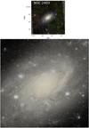 |
Fig. B.2 Same as for Fig. 1, but for NGC 2403. |
| In the text | |
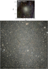 |
Fig. B.3 Same as for Fig. 1, but for NGC6822. |
| In the text | |
|
Fig. C.1 Surface brightness and color profiles extracted by AutoProf, as described in the text: Holmberg II and IC 10 in the top row; and NGC 2403 and NGC 6744 in the bottom. The four bands are given by purple, blue, green, and red for IE, YE, JE, and HE, respectively. The 1σ SB limits from AutoProf in units of mag arcsec-2 are shown as dashed horizontal lines, with colors corresponding to the Euclid bands. The fluxes have been corrected for foreground extinction (Sect. 4.1) in order to be consistent with the IE - HE radial color gradient shown in the middle panel, and YE - HE shown at the bottom. The uncorrected IE profile is shown as a dotted (purple) curve in the top panel. The mean IE - HE color over typically a factor of 100 in radius in the inner galaxy is shown as a horizontal dashed line in the middle panel. |
| In the text | |
|
Fig. D.1 Star-count maps obtained as described in Sect. 5, but for NGC 2403 (left panel), and the most distant Showcase galaxy, NGC 6744 (right). |
| In the text | |
Current usage metrics show cumulative count of Article Views (full-text article views including HTML views, PDF and ePub downloads, according to the available data) and Abstracts Views on Vision4Press platform.
Data correspond to usage on the plateform after 2015. The current usage metrics is available 48-96 hours after online publication and is updated daily on week days.
Initial download of the metrics may take a while.