| Issue |
A&A
Volume 697, May 2025
Euclid on Sky
|
|
|---|---|---|
| Article Number | A6 | |
| Number of page(s) | 43 | |
| Section | Catalogs and data | |
| DOI | https://doi.org/10.1051/0004-6361/202450803 | |
| Published online | 30 April 2025 | |
Euclid: Early Release Observations – Programme overview and pipeline for compact- and diffuse-emission photometry★
1 Université Paris-Saclay, Université Paris Cité, CEA, CNRS, AIM, 91191 Gif-sur-Yvette, France
2 INAF-Osservatorio di Astrofisica e Scienza dello Spazio di Bologna, Via Piero Gobetti 93/3, 40129 Bologna, Italy
3 Laboratoire d’Astrophysique de Bordeaux, CNRS and Université de Bordeaux, Allée Geoffroy St. Hilaire, 33165 Pessac, France
4 Institut universitaire de France (IUF), 1 rue Descartes, 75231 Paris Cedex 05, France
5 NRC Herzberg, 5071 West Saanich Rd, Victoria, BC V9E 2E7, Canada
6 Canada-France-Hawaii Telescope, 65-1238 Mamalahoa Hwy, Kamuela, HI 96743, USA
7 Max Planck Institute for Extraterrestrial Physics, Giessenbachstr. 1, 85748 Garching, Germany
8 Université Côte d’Azur, Observatoire de la Côte d’Azur, CNRS, Laboratoire Lagrange, Bd de l’Observatoire, CS 34229, 06304 Nice Cedex 4, France
9 Université de Strasbourg, CNRS, Observatoire astronomique de Strasbourg, UMR 7550, 67000 Strasbourg, France
10 Perimeter Institute for Theoretical Physics, Waterloo, Ontario N2L 2Y5, Canada
11 European Space Agency/ESTEC, Keplerlaan 1, 2201 AZ Noordwijk, The Netherlands
12 Kapteyn Astronomical Institute, University of Groningen, PO Box 800, 9700 AV Groningen, The Netherlands
13 Max-Planck-Institut für Astronomie, Königstuhl 17, 69117 Heidelberg, Germany
14 Department of Physics, Université de Montréal, 2900 Edouard Montpetit Blvd, Montréal, Québec H3T 1J4, Canada
15 Johns Hopkins University 3400 North Charles Street Baltimore, MD 21218, USA
16 Université Paris-Saclay, CNRS, Institut d’astrophysique spatiale, 91405, Orsay, France
17 ESAC/ESA, Camino Bajo del Castillo, s/n., Urb. Villafranca del Castillo, 28692 Villanueva de la Cañada, Madrid, Spain
18 Institut d’Astrophysique de Paris, UMR 7095, CNRS, and Sorbonne Université, 98 bis boulevard Arago, 75014 Paris, France
19 Sterrenkundig Observatorium, Universiteit Gent, Krijgslaan 281 S9, 9000 Gent, Belgium
20 Centro de Astrobiología (CAB), CSIC-INTA, ESAC Campus, Camino Bajo del Castillo s/n, 28692 Villanueva de la Cañada, Madrid, Spain
21 Institute of Astronomy, University of Cambridge, Madingley Road, Cambridge CB3 0HA, UK
22 Aix-Marseille Université, CNRS, CNES, LAM, Marseille, France
23 INAF - Osservatorio Astronomico di Cagliari, Via della Scienza 5, 09047 Selargius (CA), Italy
24 David A. Dunlap Department of Astronomy & Astrophysics, University of Toronto, 50 St George Street, Toronto, Ontario M5S 3H4, Canada
25 Jodrell Bank Centre for Astrophysics, Department of Physics and Astronomy, University of Manchester, Oxford Road, Manchester M13 9PL, UK
26 Departamento de Física Teórica, Atómica y Óptica, Universidad de Valladolid, 47011 Valladolid, Spain
27 Instituto de Astrofísica e Ciências do Espaço, Faculdade de Ciências, Universidade de Lisboa, Tapada da Ajuda, 1349-018 Lisboa, Portugal
28 INAF - Osservatorio Astronomico d’Abruzzo, Via Maggini, 64100 Teramo, Italy
29 INAF-Osservatorio Astronomico di Trieste, Via G. B. Tiepolo 11, 34143 Trieste, Italy
30 School of Mathematics and Physics, University of Surrey, Guildford, Surrey GU2 7XH, UK
31 Institute for Astronomy, University of Edinburgh, Royal Observatory, Blackford Hill, Edinburgh EH9 3HJ, UK
32 Department of Mathematics and Physics E. De Giorgi, University of Salento, Via per Arnesano, CP-I93, 73100 Lecce, Italy
33 INFN, Sezione di Lecce, Via per Arnesano, CP-193, 73100 Lecce, Italy
34 INAF-Sezione di Lecce, c/o Dipartimento Matematica e Fisica, Via per Arnesano, 73100 Lecce, Italy
35 Instituto de Física de Cantabria, Edificio Juan Jordá, Avenida de los Castros, 39005 Santander, Spain
36 INAF-Osservatorio Astronomico di Roma, Via Frascati 33, 00078 Monteporzio Catone, Italy
37 Observatorio Nacional, Rua General Jose Cristino, 77-Bairro Imperial de Sao Cristovao, Rio de Janeiro 20921-400, Brazil
38 Departamento de Física, Faculdade de Ciências, Universidade de Lisboa, Edifício C8, Campo Grande, 1749-016 Lisboa, Portugal
39 Instituto de Astrofísica e Ciências do Espaço, Faculdade de Ciências, Universidade de Lisboa, Campo Grande, 1749-016 Lisboa, Portugal
40 Universidad de La Laguna, Departamento de Astrofísica, 38206 La Laguna, Tenerife, Spain
41 Instituto de Astrofísica de Canarias, Vía Láctea, 38205 La Laguna, Tenerife, Spain
42 Universitäts-Sternwarte München, Fakultät für Physik, Ludwig-Maximilians-Universität München, Scheinerstrasse 1, 81679 München, Germany
43 Aix-Marseille Université, CNRS/IN2P3, CPPM, Marseille, France
44 School of Physics and Astronomy, University of Nottingham, University Park, Nottingham NG7 2RD, UK
45 International Space University, 1 rue Jean-Dominique Cassini, 67400 Illkirch-Graffenstaden, France
46 Department of Astronomy, University of Florida, Bryant Space Science Center, Gainesville, FL 32611, USA
47 Department of Astronomy, University of Geneva, ch. d’Ecogia 16, 1290 Versoix, Switzerland
48 INAF-Osservatorio Astrofisico di Arcetri, Largo E. Fermi 5, 50125 Firenze, Italy
49 Institute of Physics, Laboratory of Astrophysics, Ecole Polytechnique Fédérale de Lausanne (EPFL), Observatoire de Sauverny, 1290 Versoix, Switzerland
50 Department of Physics, Centre for Extragalactic Astronomy, Durham University, South Road, Durham DH1 3LE, UK
51 Department of Physics, Institute for Computational Cosmology, Durham University, South Road, Durham DH1 3LE, UK
52 Astrophysics Research Centre, University of KwaZulu-Natal, Westville Campus, Durban 4041, South Africa
53 School of Mathematics, Statistics & Computer Science, University of KwaZulu-Natal, Westville Campus, Durban 4041, South Africa
54 National Astronomical Observatory of Japan, 2-21-1 Osawa, Mitaka, Tokyo 181-8588, Japan
55 Department of Astrophysics/IMAPP, Radboud University, PO Box 9010, 6500 GL Nijmegen, The Netherlands
56 Aurora Technology for European Space Agency (ESA), Camino bajo del Castillo, s/n, Urbanizacion Villafranca del Castillo, Villanueva de la Cañada, 28692 Madrid, Spain
57 HE Space for European Space Agency (ESA), Camino bajo del Castillo, s/n, Urbanizacion Villafranca del Castillo, Villanueva de la Cañada, 28692 Madrid, Spain
58 Universität Innsbruck, Institut für Astro- und Teilchenphysik, Technikerstr. 25/8, 6020 Innsbruck, Austria
59 INFN-Sezione di Bologna, Viale Berti Pichat 6/2, 40127 Bologna, Italy
60 Leiden Observatory, Leiden University, Einsteinweg 55, 2333 CC Leiden, The Netherlands
61 Departamento de Física de la Tierra y Astrofísica, Universidad Complutense de Madrid, Plaza de las Ciencias 2, 28040 Madrid, Spain
62 Kobayashi-Maskawa Institute for the Origin of Particles and the Universe, Nagoya University, Chikusa-ku, Nagoya 464-8602, Japan
63 Institute for Advanced Research, Nagoya University, Chikusa-ku, Nagoya 464-8601, Japan
64 Kavli Institute for the Physics and Mathematics of the Universe (WPI), University of Tokyo, Kashiwa, Chiba 277-8583, Japan
65 European Space Agency, 8-10 rue Mario Nikis, 75738 Paris Cedex 15, France
66 Niels Bohr Institute, University of Copenhagen, Jagtvej 128, 2200 Copenhagen, Denmark
67 Cosmic Dawn Center (DAWN), Denmark
68 Center for Frontier Science, Chiba University, 1-33 Yayoi-cho, Inage-ku, Chiba 263-8522, Japan
69 Department of Physics, Graduate School of Science, Chiba University, 1-33 Yayoi-Cho, Inage-Ku, Chiba 263-8522, Japan
70 Space physics and astronomy research unit, University of Oulu, Pentti Kaiteran katu 1, 90014 Oulu, Finland
71 Centre de Recherche Astrophysique de Lyon, UMR5574, CNRS, Université Claude Bernard Lyon 1, ENS de Lyon, 69230, Saint-Genis-Laval, France
72 European Southern Observatory, Karl-Schwarzschild-Str. 2, 85748 Garching, Germany
73 Jet Propulsion Laboratory, California Institute of Technology, 4800 Oak Grove Drive, Pasadena, CA 91109, USA
74 School of Physics & Astronomy, University of Southampton, High-field Campus, Southampton SO17 1BJ, UK
75 School of Physical Sciences, The Open University, Milton Keynes, MK7 6AA, UK
76 Univ. Lille, CNRS, Centrale Lille, UMR 9189 CRIStAL, 59000 Lille, France
77 Leibniz-Institut für Astrophysik (AIP), An der Sternwarte 16, 14482 Potsdam, Germany
78 INAF-Osservatorio Astronomico di Capodimonte, Via Moiariello 16, 80131 Napoli, Italy
79 Department of Astronomy, University of Massachusetts, Amherst, MA 01003, USA
80 INAF-Osservatorio Astronomico di Brera, Via Brera 28, 20122 Milano, Italy
81 IFPU, Institute for Fundamental Physics of the Universe, via Beirut 2, 34151 Trieste, Italy
82 INFN, Sezione di Trieste, Via Valerio 2, 34127 Trieste TS, Italy
83 SISSA, International School for Advanced Studies, Via Bonomea 265, 34136 Trieste TS, Italy
84 Dipartimento di Fisica e Astronomia, Università di Bologna, Via Gobetti 93/2, 40129 Bologna, Italy
85 INAF-Osservatorio Astronomico di Padova, Via dell’Osservatorio 5, 35122 Padova, Italy
86 Centre National d’Etudes Spatiales - Centre spatial de Toulouse, 18 avenue Edouard Belin, 31401 Toulouse Cedex 9, France
87 Dipartimento di Fisica, Università di Genova, Via Dodecaneso 33, 16146, Genova, Italy
88 INFN-Sezione di Genova, Via Dodecaneso 33, 16146 Genova, Italy
89 Institut de Recherche en Astrophysique et Planétologie (IRAP), Université de Toulouse, CNRS, UPS, CNES, 14 Av. Edouard Belin, 31400 Toulouse, France
90 Department of Physics “E. Pancini”, University Federico II, Via Cinthia 6, 80126 Napoli, Italy
91 INFN section of Naples, Via Cinthia 6, 80126 Napoli, Italy
92 Instituto de Astrofísica e Ciências do Espaço, Universidade do Porto, CAUP, Rua das Estrelas, 4150-762 Porto, Portugal
93 Faculdade de Ciências da Universidade do Porto, Rua do Campo de Alegre, 4150-007 Porto, Portugal
94 Dipartimento di Fisica, Università degli Studi di Torino, Via P. Giuria 1, 10125 Torino, Italy
95 INFN-Sezione di Torino, Via P. Giuria 1, 10125 Torino, Italy
96 INAF-Osservatorio Astrofisico di Torino, Via Osservatorio 20, 10025 Pino Torinese (TO), Italy
97 INAF-IASF Milano, Via Alfonso Corti 12, 20133 Milano, Italy
98 Centro de Investigaciones Energéticas, Medioambientales y Tecnológicas (CIEMAT), Avenida Complutense 40, 28040 Madrid, Spain
99 Port d’Informació Científica, Campus UAB, C. Albareda s/n, 08193 Bellaterra (Barcelona), Spain
100 Institute for Theoretical Particle Physics and Cosmology (TTK), RWTH Aachen University, 52056 Aachen, Germany
101 Institute of Space Sciences (ICE, CSIC), Campus UAB, Carrer de Can Magrans, s/n, 08193 Barcelona, Spain
102 Institut d’Estudis Espacials de Catalunya (IEEC), Edifici RDIT, Campus UPC, 08860 Castelldefels, Barcelona, Spain
103 Dipartimento di Fisica e Astronomia “Augusto Righi” - Alma Mater Studiorum Università di Bologna, Viale Berti Pichat 6/2, 40127 Bologna, Italy
104 European Space Agency/ESRIN, Largo Galileo Galilei 1, 00044 Frascati, Roma, Italy
105 Université Claude Bernard Lyon 1, CNRS/IN2P3, IP2I Lyon, UMR 5822, Villeurbanne 69100, France
106 UCB Lyon 1, CNRS/IN2P3, IUF, IP2I Lyon, 4 rue Enrico Fermi, 69622 Villeurbanne, France
107 Mullard Space Science Laboratory, University College London, Holmbury St Mary, Dorking, Surrey RH5 6NT, UK
108 INAF-Istituto di Astrofisica e Planetologia Spaziali, via del Fosso del Cavaliere, 100, 00100 Roma, Italy
109 INFN-Padova, Via Marzolo 8, 35131 Padova, Italy
110 School of Physics, HH Wills Physics Laboratory, University of Bristol, Tyndall Avenue, Bristol BS8 1TL, UK
111 Istituto Nazionale di Fisica Nucleare, Sezione di Bologna, Via Irnerio 46, 40126 Bologna, Italy
112 FRACTAL S.L.N.E., calle Tulipán 2, Portal 13 1A, 28231 Las Rozas de Madrid, Spain
113 Dipartimento di Fisica “Aldo Pontremoli”, Università degli Studi di Milano, Via Celoria 16, 20133 Milano, Italy
114 Institute of Theoretical Astrophysics, University of Oslo, PO Box 1029 Blindern, 0315 Oslo, Norway
115 Department of Physics, Lancaster University, Lancaster LA1 4YB, UK
116 Felix Hormuth Engineering, Goethestr. 17, 69181 Leimen, Germany
117 Technical University of Denmark, Elektrovej 327, 2800 Kgs. Lyngby, Denmark
118 Cosmic Dawn Center (DAWN), Denmark
119 NASA Goddard Space Flight Center, Greenbelt, MD 20771, USA
120 Department of Physics and Helsinki Institute of Physics, Gustaf Hällströmin katu 2, 00014 University of Helsinki, Finland
121 Université de Genève, Département de Physique Théorique and Centre for Astroparticle Physics, 24 quai Ernest-Ansermet, 1211 Genève 4, Switzerland
122 Department of Physics, PO Box 64, 00014 University of Helsinki, Finland
123 Helsinki Institute of Physics, Gustaf Hällströmin katu 2, University of Helsinki, Helsinki, Finland
124 Department of Physics and Astronomy, University College London, Gower Street, London WC1E 6BT, UK
125 NOVA optical infrared instrumentation group at ASTRON, Oude Hoogeveensedijk 4, 7991PD Dwingeloo, The Netherlands
126 INFN-Sezione di Milano, Via Celoria 16, 20133 Milano, Italy
127 Universität Bonn, Argelander-Institut für Astronomie, Auf dem Hügel 71, 53121 Bonn, Germany
128 Dipartimento di Fisica e Astronomia “Augusto Righi” - Alma Mater Studiorum Università di Bologna, via Piero Gobetti 93/2, 40129 Bologna, Italy
129 Institut d’Astrophysique de Paris, 98bis Boulevard Arago, 75014, Paris, France
130 Institut de Física d’Altes Energies (IFAE), The Barcelona Institute of Science and Technology, Campus UAB, 08193 Bellaterra (Barcelona), Spain
131 Department of Physics and Astronomy, University of Aarhus, Ny Munkegade 120, DK-8000 Aarhus C, Denmark
132 Waterloo Centre for Astrophysics, University of Waterloo, Waterloo, Ontario N2L 3G1, Canada
133 Department of Physics and Astronomy, University of Waterloo, Waterloo, Ontario N2L 3G1, Canada
134 Space Science Data Center, Italian Space Agency, via del Politecnico snc, 00133 Roma, Italy
135 Institute of Space Science, Str. Atomistilor, nr. 409 Măgurele, Ilfov, 077125, Romania
136 Institute for Particle Physics and Astrophysics, Dept. of Physics, ETH Zurich, Wolfgang-Pauli-Strasse 27, 8093 Zurich, Switzerland
137 Dipartimento di Fisica e Astronomia “G. Galilei”, Università di Padova, Via Marzolo 8, 35131 Padova, Italy
138 Departamento de Física, FCFM, Universidad de Chile, Blanco Encalada 2008, Santiago, Chile
139 Satlantis, University Science Park, Sede Bld 48940, Leioa-Bilbao, Spain
140 Centre for Electronic Imaging, Open University, Walton Hall, Milton Keynes MK7 6AA, UK
141 Infrared Processing and Analysis Center, California Institute of Technology, Pasadena, CA 91125, USA
142 Universidad Politécnica de Cartagena, Departamento de Electrónica y Tecnología de Computadoras, Plaza del Hospital 1, 30202 Cartagena, Spain
143 Centre for Information Technology, University of Groningen, PO Box 11044, 9700 CA Groningen, The Netherlands
144 INFN-Bologna, Via Irnerio 46, 40126 Bologna, Italy
145 INAF, Istituto di Radioastronomia, Via Piero Gobetti 101, 40129 Bologna, Italy
146 ICL, Junia, Université Catholique de Lille, LITL, 59000 Lille, France
147 Department of Physics and Astronomy, University of British Columbia, Vancouver, BC V6T 1Z1, Canada
★★ Corresponding author; jc.cuillandre@cea.fr
Received:
20
May
2024
Accepted:
26
February
2025
The Euclid Early Release Observations (ERO) showcase Euclid’s capabilities in advance of its main mission by targeting 17 astronomical objects, including galaxy clusters, nearby galaxies, globular clusters, and star-forming regions. A total of 24 hours of observing time was allocated in the early months of operation, and the scientific community was engaged through an early public data release. We describe the development of the ERO pipeline to create visually compelling images while simultaneously meeting the scientific demands within months of launch by leveraging a pragmatic data-driven development strategy. The pipeline’s key requirements are to preserve the image quality and to provide flux calibration and photometry for compact and extended sources. The pipeline’s five pillars are removal of instrumental signatures, astrometric calibration, photometric calibration, image stacking, and the production of science-ready catalogues for both the VIS and NISP instruments. We report a point spread function (PSF) with a full width at half maximum of 0ʺ.16 in the optical IE-band and 0ʺ.49 in the near-infrared (NIR) bands YE, JE, and HE. Our VIS mean absolute flux calibration is accurate to about 1%, and the accuracy is 10% for NISP due to a limited calibration set; both instruments have considerable colour terms for individual sources. The median depth is 25.3 and 23.2 AB mag with a signal-to-noise ratio (S/N) of ten for galaxies, while it is 27.1 and 24.5 AB mag at an S/N of five for point sources for VIS and NISP, respectively. Euclid’s ability to observe diffuse emission is exceptional due to its extended PSF nearly matching a pure diffraction halo, the best ever achieved by a wide-field high-resolution imaging telescope. Euclid offers unparalleled capabilities for exploring the low-surface brightness (LSB) Universe across all scales, providing high precision within a wide field of view (FoV), and opening a new observational window in the NIR. Median surface-brightness levels of 29.5 and 27.9, AB mag arcsec−2 are achieved for VIS and NISP, respectively, for detecting a 10ʺ × 10ʺ extended feature at the 1 σ level.
Key words: space vehicles: instruments / techniques: image processing / techniques: photometric / catalogs / astrometry
© The Authors 2025
 Open Access article, published by EDP Sciences, under the terms of the Creative Commons Attribution License (https://creativecommons.org/licenses/by/4.0), which permits unrestricted use, distribution, and reproduction in any medium, provided the original work is properly cited.
This article is published in open access under the Subscribe to Open model. Subscribe to A&A to support open access publication.
1 Introduction
Euclid is an ongoing space mission, part of the European Space Agency (ESA) Cosmic Vision programme, originating from a 2007 call for a medium-size mission. Euclid spawned from proposals focused on dark energy and is now conducting an extragalactic survey using optical imaging and NIR imaging and spectroscopy. The mission’s six-year survey is designed to study galaxy clustering and weak gravitational lensing, providing essential probes of the Universe’s large-scale structure and the processes that govern its expansion. The primary scientific objectives are outlined in a key publication that led to the mission’s official selection and adoption by ESA in 2011 and 2012 (Laureijs et al. 2011), respectively. Euclid was successfully launched on 1 July 2023. Euclid Collaboration: Mellier et al. (2025) describes the spacecraft, discusses the mission’s early phase in orbit, its survey strategy, the data it collects, and the scientific research it enables. The two scientific instruments VIS and the Near-Infrared Spectrometer and Photometer (NISP) are described in great depth in Euclid Collaboration: Cropper et al. (2025) and Euclid Collaboration: Schirmer et al. (2025), respectively. These three defining articles from the Euclid Consortium act as a cornucopia of Euclid knowledge.
The Early Release Observations (ERO) programme is a special project by the ESA Euclid science team aimed at gathering and sharing scientific observations for public engagement and communication purposes before the main mission activities start (Euclid Early Release Observations 2024). The goal is to highlight Euclid’s capabilities through visually engaging astronomical objects that are not central to the mission’s core cosmological goals. This has entailed observations of extended objects that fill most of Euclid’s large FoV and naturally led to the selection of proposals from the Euclid scientific community that showcased nearby objects. For the ERO programme, the science team considered the inclusion of objects at increasing distances to cover the rich variety of science topics that can be addressed. The ERO sequence starts with Galactic nebulae in the Orion star-forming region at a distance of 500 pc (Martín et al. 2025). These are followed by globular clusters in the Milky Way (Massari et al. 2025), nearby galaxies (Hunt et al. 2025), and more distant galaxy clusters, with the nearest being the Dorado and Fornax clusters (Saifollahi et al. 2025) at 15–20 Mpc. Subsequently, the ERO sequence continues to the Perseus cluster at 72 Mpc (Cuillandre et al. 2025; Kluge et al. 2025; Marleau et al. 2025), and last are the two Abell clusters, with the most distant one at z = 0.228 (Atek et al. 2025). Since these observations are not part of the main mission, there was a push to publicly release the collected data to the scientific community as quickly as possible. Due to the focus on unique sky regions containing extended emission not covered by the main survey together with the quick turnaround needed for public communication, the ERO data set was processed differently than the nominal Euclid survey data.
In this paper, we describe in Sect. 2 the objectives and methods of ERO. In Sect. 3, we focus on the ERO pipeline strategy and implementation, highlighting the pipeline’s origins and requirements, and this is followed by discussion of our implementation strategy. In Sect. 4, we focus on image detrending, an essential step for preparing the images for scientific analysis. This part is comprehensive, starting with the ingestion and initial evaluation of the ERO images. For the detrending of the optical VIS data, we explain the procedures for correcting bad pixels, overscan, bias structure, dark current, and stray light as well as for applying flat-field corrections, detector-to-detector image scaling, and identifying and removing cosmic rays (CRs). Similarly, for detrending NIR data from the NISP instrument, we cover charge-persistence correction, bad-pixel masks, electronic pedestal correction, dark current correction, flat-field correction, row correlated-noise correction, and CRs. The astrometric calibration follows in Sect. 5, where we outline the process to accurately anchor the data to the Gaia data release 3 (DR3) astrometric reference (Gaia Collaboration 2016, 2023). We describe in Sect. 6 our resampling and stacking methods, and we cover the photometric calibration for both instruments in Sect. 7. In Sect. 8, using compact-source catalogues and general performance of the ERO data, we examine PSF modelling and the production of the science-validation catalogues, and we provide a performance summary of the ERO data to assess their scientific utility. In Sect. 9, we assess the performance for LSB science in support of the early science conducted with the ERO images. We derive the extended PSF in all four Euclid bands. This involves studying a simple model of the optical design, modelling the encompassed energy of the PSF, and evaluating the consequences for the ERO LSB science cases.
The paper concludes in Sect. 10 with an executive summary that encapsulates the main points and findings showcased. We first present in Appendix A a concise summary of the ERO data. Appendix B then presents two complete tables summarising details of the ERO data set (depth, etc.). In Appendix C, we discuss the selection of relevant stars along a given line of sight for identifying and cataloguing stars for follow-up studies. Lastly, in Appendix D, we describe the optical model of the telescope used to compare with the extended PSF derived in Sect. 9.
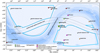 |
Fig. 1 Location, name, and nature of the 17 ERO fields on an all-sky map. The general RoI of the EWS is highlighted by the four blue contours. These outlines signify that some of the ERO targets will be revisited in the coming years. The distinctive nature of the ERO programme facilitated explorations spanning from the Galactic plane to the southern Galactic cap, areas that were accessible during the observation period. This range of coverage showcases the ERO programme’s goal to venture across a wide variety of astronomical phenomena and regions. The blue background depicts the stellar density across the sky. |
2 Euclid ERO overview
2.1 Programme description
The ERO programme was an initiative by the Euclid science team. At inception, we aimed to acquire scientific observations for communication and early scientific results purposes before the nominal mission begins. Through the ERO programme, we aimed to showcase the unique instrumental capabilities of Euclid by selecting large and nearby astronomical targets that are completely separate from the cosmological objectives of Euclid. We seized the opportunity to schedule specific fields in the sky during the early operations phase, ensuring our activities did not interfere with the planning process of the nominal survey and allowing us a greater degree of operational flexibility. Since this programme fell outside the scope of the nominal mission, we committed to making the resulting scientific data products publicly available as promptly as possible.
In March 2023, we issued a call for proposals to the Euclid Collaboration. The total time allocated was limited to 24 accumulated hours. After evaluating the visibility of the fields during the performance-verification (PV) phase and ensuring the absence of nearby overly bright stars, we ranked the proposals based on their societal impact merit, scientific merit, and uniqueness. The selected proposals and their approved targets are listed in Table A.1.
Due to the focused attention on non-standard Euclid fields outside the main mission survey area (Fig. 1) and the relatively short timescales for preparing communication products, we handled the processing and release of the data products separately from the development of the Euclid science ground segment. The ERO image processing drew on common knowledge and extensive experience in astronomical imaging with charge-coupled devices (CCDs) and HAWAII-2RG (H2RG) HgCdTe sensors, akin to those used by VIS and NISP, respectively. The ERO programme required the use of the reference observing sequences (ROSs), which are the building blocks of the EWS described in Euclid Collaboration: Scaramella et al. (2022) and Euclid Collaboration: Mellier et al. (2025). Each ROS also collects slitless spectra. Given the tight schedule and reliance on common knowledge, we could not process the spectroscopic data in time for inclusion in the first public data release.
2.2 Observing strategy
The ROS provides a single standard EWS field together with a range of inline calibration data. It has been highly optimised to provide a maximum amount of scientific data in a minimum amount of time, in a consistent way during the entire six-year survey; it guarantees a sufficient S/N and depth for Euclid’s core science. The ERO programme permitted multiple ROS observations of certain fields to enhance the depth. Additionally, the programme allowed for observations outside the RoI, which delineates the useful extragalactic sky area for the wide and deep surveys (Fig. 1).
The ROS comprises four dithers on every field to fill the detector gaps. For each dither, the same measurement sequence is executed. First comes a VIS IE-band nominal-science exposure of 566 s, with a concurrent NISP spectroscopic exposure of 574 s in one of the four red-grism orientations. These are followed by a sequence of three NISP images in the JE, HE, and YE bands, each lasting 112 s. For the ERO programme, each dither also included an IE short-science exposure of 95 s simultaneously to the YE exposure, yielding four such images per ROS; for the EWS, two of the VIS short-science exposures are replaced by VIS calibration images (see Euclid Collaboration: Mellier et al. 2025).
The ERO fields were scheduled during the available time slots in the PV phase dedicated to calibration observations. The PV phase commenced on 6 August 2023 and concluded on 3 December 2023. The pre-launch allocation for the PV phase was two months; however, it was soon interrupted due to failures of the spacecraft’s fine guidance sensor (FGS) in fields with a low density of suitable guide stars. PV observations resumed on 28 September 2023 after concluding the development and validation of improved FGS software. Prior to this date, we proceeded with observing ERO fields that were about to lose their visibility, accepting the risk of poor guiding for some or all exposures in these fields. The programme allowed observation of suitable backup sources in case fields were lost due to closure of their visibility window or an operational anomaly.
2.3 Summary of the observations
A summary of the observed ERO fields is provided in Table A.1. Observations conducted before 28 September 2023 – which covered high stellar density fields such as the globular cluster NGC 6254, the irregular galaxy IC 10, and the Perseus galaxy cluster – were unaffected by the FGS anomaly. However, for the reflection nebula NGC 1333, the Fornax galaxy cluster, and one ROS on the Taurus molecular cloud, only a limited number of exposures per ROS achieved the required guiding performance. Despite this, the Fornax galaxy cluster, observed during three epochs, yielded a sufficient number of good exposures in all four bands to enable scientific analysis.
All ROS observations carried out before 16 September 2023, were executed with a dither pattern mistakenly rotated by 90° due to early spacecraft operations. This resulted in zero-coverage gaps in the VIS and NISP stacked images, attributable to the lack of sensor coverage from either VIS or NISP. These gaps account for a few percent of the total field area, yet the exposures remain viable for scientific investigation.
3 ERO pipeline strategy and implementation
3.1 Origins and requirements
The ERO pipeline was initially developed to create aesthetically striking images of astronomical sources within three months of the telescope’s launch, celebrating the advent of a new telescope. The objective was to occupy a significant portion of the Euclid FoV with large, colourful objects. Such objects are categorised as extended emission, whether due to their combined stellar density (as in a globular cluster), their nebulous nature (star-forming regions), or their diffuse aspect (unresolved stars), encompassing both high and lowsurface-brightness sources. Throughout this reduction process, it was imperative that the images highlight Euclid’s unparalleled sharpness from the optical to the NIR across such a large FoV.
Prior to launch, the project rapidly evolved to address the need for the early public release of associated scientific data and related science results. Given that many of the proposed science projects depended on the precise measurement of physical properties derived from extended emission, an alternate approach to the official scientific processing of Euclid data was required. Consequently, the ERO pipeline was tasked with delivering both outreach images and scientific products for all six ERO science teams (see Table A.1). The minimum requirements for the quality of processing and calibration at the onset of the effort have been met and some exceeded as detailed in this paper. This achievement has facilitated a rich early showcase of Euclid science, highlighting its unique observing capabilities.
Creating images for early release to the world necessitated starting from raw data to produce contiguous images of the sky that are free of visual flaws, such as detector mosaic gaps, CRs, detector persistence, and variations in detector sensitivity, among others. These requirements also enhanced the production of science-ready products. The ERO pipeline adeptly managed both domains, with the outreach effort diverging partway through the process. This divergence occurs post-detrending, a step that is detailed below. The subsequent steps involved in producing visually engaging images are not the focus of this paper, which is dedicated to the production of science products.
The selected science projects drove the ultimate requirements for the development of the ERO pipeline:
preservation of the intrinsic delivered image quality;
correction of optical distortions to anchor on the world coordinate system (WCS);
uniformity of the flux calibration across the FoV;
photometry of compact sources and extended emission;
matched processing for the two instruments (VIS and NISP).
These fundamental requirements translated into the five main pillars of the ERO pipeline, based on the adoption of a uniform set of image processing tools:
optimal removal of instrumental signatures (detrending);
astrometric calibration (internal and absolute);
photometric calibration (internal and external);
stacking of images into a contiguous region of the sky;
production of science-ready catalogues based on the stacks.
3.2 Implementation strategy
Due to the tight schedule (3 months to deliver images and the first science data release, 6 months for final products for the first science publications), we adopted for the detrending part the existing C code pipeline developed for similar optical and NIR wide-field imaging instruments operated over the past couple of decades at the Canada-France-Hawaii Telescope (CFHT): MegaCam (Magnier & Cuillandre 2004) and WIRCam (Pipien et al. 2018). For astrometric calibration, stacking, PSF modelling, and source extraction, we chose the AstrOmatic suite (Bertin & Arnouts 1996; Bertin et al. 2002; Bertin 2006), widely adopted across the scientific community. Many of its developments have been driven by these two CFHT instruments as well, making them particularly well-suited for Euclid’s wide- field imaging data. Additional key community-based resources adopted in the ERO pipeline include Astrometry.net (Lang et al. 2010), and various Python packages such as deepCR (Zhang & Bloom 2020).
The short timescale of the ERO programme necessitated a pragmatic approach to the development of the custom pipeline, including enhancements of some AstrOmatic tools to fully leverage the data set’s quality. Development of the ERO pipeline commenced within weeks of the first space data availability post-launch. The tight schedule mandated the formulation and optimisation of processing recipes based on an empirical, data- driven approach, without prior knowledge of the specifics of the Euclid instruments and detectors. Consequently, the resulting ERO pipeline, with relaxed requirements for photometry of compact sources and more stringent ones for extended sources, was bound to be inherently distinct and entirely separate from the main mission pipeline.
The following sections address all aspects that led to the ERO science products for both VIS and NISP: data detrending, astrometric calibration, photometric calibration, stacking, PSF extraction, and catalogue production.
4 Image detrending
All detector effects described in this section are – to various extents – common to CCDs and H2RGs architectures. However, due to the very low background and the presence of space weather, some of the effects are more important for Euclid than for a ground-based observatory.
4.1 Ingestion and initial evaluation of the ERO images
The initial stage in the ERO pipeline involved enhancing Level 1 Euclid (LE1) multi-extension FITS (MEF) images for both VIS and NISP. Specifically, we incorporated keywords that help delineate the physical coordinates of particular pixel regions, such as prescan and overscan areas, and the active imaging pixels within each detector (e.g. PRESCAN, OVERSCAN, BIASSEC, DATASEC), and provide details about their physical layout within the detector mosaic (e.g. DETSIZE, DETSEC). Utilising the libfh library1 from the CFHT, this step generates a new MEF file that preserves the original structure of 144 extensions for VIS and 16 for NISP. Simultaneously, it compiles detailed statistics about the images (such as bias levels and overall image quality), creates JPEG previews, and fills a text-based database with a comprehensive summary of key attributes for each Euclid image. This database created within days of the observations became a crucial resource for all later stages of the pipeline.
Upon the availability of various previews, the pipeline began a preliminary visual validation process aimed at identifying and excluding images affected by sub-optimal guiding. This step involved enhancing the database with validation flags. Notably, to support the development of the ERO pipeline, data from both the commissioning phase and PV activities conducted alongside the ERO observation period were integrated into the ERO database.
4.2 Detrending optical data from the VIS instrument
VIS comprises 36 Teledyne e2V CCD273-84 CCDs arranged in a 6 × 6 mosaic, with a plate scale of 0ʺ.1 pixel−1 and 4096 × 4132 pixel per detector. The instrument and its detector properties are described in detail in Euclid Collaboration: Cropper et al. (2025).
4.2.1 Bad pixel masks
The cosmetic quality of the CCDs is excellent, necessitating minimal masking for single bad pixels, clusters of bad pixels, and blocked columns. Such pixels that do need to be masked were identified through their nonlinear response by comparing an internal calibration light-emitting diode (LED) illumination image of 30 000 analogue-to-digital units (ADUs) with one at 1/10th that intensity; deviations above or below a 1.2% threshold led to masking. Furthermore, as a conservative measure for photometry accuracy, we masked five lines at the bottom and four lines at the top of each of the four imaging quadrants per CCD (with four parallel readouts, each quadrant measures 2048 × 2066 pixels). This action was necessary due to slight nonlinearity issues related to the geometry of the pixels at the top of the quadrant, influenced by the presence of an injection charge channel in the middle of the CCD, and the slight instability in the electronic chains at the start of readout for the bottom lines. Overall, the ERO pipeline mask (0/1) affects merely 0.53% of all imaging pixels, with a significant portion (0.44%) originating from the nine lines masked per quadrant.
4.2.2 Overscan correction
Close examination of the overscan region per quadrant (28 columns wide extra readout cycles per line once all pixels from the serial register containing imaging data have been read out) revealed a subtle modulation at the roughly 1 ADU level across scales of 50 pixels along the vertical axis. The median electronic gain of VIS is 3.5 electrons per ADU, indicating slow fluctuations at the 3–4 electrons level of the readout pedestal drift. This phenomenon is linked to a temporal instability in the readout electronic chains on a timescale of seconds throughout the 72-s-long readout. This random effect is believed to be caused by the power supply, which generates faint ripples during the readout. These ripples occur at a wide range of frequencies, affecting anything from individual lines to several hundred lines, and can have an amplitude of up to 1 ADU in that second regime. Sudden transitions to high signals – for example saturated stars – can also cause jumps on the order of 1 ADU during the readout. A typical 566-s VIS integration is dominated by the background from zodiacal light, at a median level of 40 ADUs in the ERO raw data (this translates to 22.2 mag arcsec−2). This modulation of the readout pedestal, constituting a third of the photon-noise level, was evident in all raw VIS images (Fig. 3, left) and required correction. It is effectively mitigated in the ERO pipeline by subtracting a vector from each column of the imaging area. This median vector was constructed for each quadrant per image across the overscan and smoothed by a 50-pixel tall median filter, matching the typical scale of modulation. Subtracting this vector from each column in the imaging area corrected the intrinsic additive pedestal introduced by the electronic chain in a single step. Since this slow modulation varies from exposure to exposure, it cannot be accounted for in a median bias, necessitating per-exposure execution. This correction of the electronic pedestal does not impact the noise properties of the images on small (pixel) scales, while significantly enhancing the overall background flatness of the VIS images (see Fig. 2).
4.2.3 Bias structure correction
The overscan correction eliminates the varying electronic pedestal, but various low- and high-frequency structures can still be observed on an overscan-corrected bias frame (right panel of Fig. 2), indicating the need to remove two-dimensional structures by subtracting a master bias image. Two CCDs in the mosaic exhibit a particularly high pedestal level due to a glow from the serial register protection circuitry when clocking the serial register, adding a signal of up to 0.6 ADU to the pixels of those detectors. A similar effect is seen at a lower level (0.1 to 0.3 ADU maximum) across the other 34 CCDs. This systematic additive effect is effectively mitigated by subtracting a full bias (2-dimensional array) constructed from a median of over 100 bias frames, initially corrected for their overscan level (see Fig. 3). Oscillations in amplitude over the first 100 pixels at the start of each line readout (ringing) are attributed to the electronic chains stabilising after each end-of-line reset operation. This purely additive effect is corrected through this process. Following overscan and bias correction of science images, the noise properties remain unaffected, with the contribution of the native readout noise of 3.2 electrons (0.93 ADU, with a dispersion of 0.06 across all 144 outputs) unchanged.
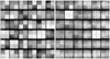 |
Fig. 2 Left: single raw VIS bias frame captured at L2. The image exhibits numerous CRs, and has been corrected with a fixed pedestal level per quadrant based on the median value in the overscan area. Right: correction using a smoothed vertical vector of the overscan area. The contrast here is maximised to highlight effects at the sub-ADU level. The solution adopted on the right still exhibits an instrumental signature (some quadrants, or entire detectors, have a non-zero signal), necessitating an additional two-dimensional bias correction. |
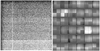 |
Fig. 3 Left: features of a CCD quadrant. This quadrant from a raw bias image shows (i) a noticeable jump in the readout pedestal during readout (with more subtle variations observable throughout the readout), (ii) a top-down intensity gradient indicative of light injection during readout, and (iii) an electronic ringing effect on the left at the start of each line readout. Right: high-S/N master bias frame (median of tens of raw images) used to process all ERO data. The brightness variation here does not exceed 0.6 ADU, while the typical raw ERO signal – zodiacal light background – is around 40 ADUs, necessitating this correction. |
4.2.4 Dark current and stray light
At the operational temperature in space, approximately 150 K, dark-current generation is negligible compared to all other sources, especially the dominant zodiacal light. The signature of dark current is undetectable in the space data at the sub-ADU level, and consequently, no correction is applied.
Stray light, an additive contaminant that occurs even with the VIS shutter closed, severely affected early commissioning data (Euclid Collaboration: Mellier et al. 2025). Positioning the spacecraft safely with respect to the Sun during the ERO programme reduced this contamination to a negligible level, except for the very first and two very last fields, Fornax, Dorado and Holmberg II, which were captured under borderline conditions. The current version of the ERO pipeline, used for our first scientific publications, does not yet incorporate this correction, and those two fields should be treated cautiously when exploring their LSB features at the 28–30 mag arcsec−2 level; we note that all magnitudes in this paper are in the AB system (Oke & Gunn 1983). The stray light correction for these three fields will be implemented in the next ERO data release.
4.2.5 Flat-field correction for large and small scales
A fundamental aspect of the ERO pipeline strategy is the zodiacal light flat-field, based on the principle that the zodiacal light at L2 is the flattest light source observable across the entire sky. The dust in the ecliptic plane scatters sunlight, producing a glowing haze with a well-modelled behaviour (see Figure 12 in Euclid Collaboration: Scaramella et al. 2022). This distribution peaks at the ecliptic plane and diminishes rapidly, averaging 22.1 mag arcsec−2 across the 17 ERO fields. Beyond an ecliptic latitude of 15°, the distribution’s steepest part shows a brightness slope of 0.007 MJy sr−1 per latitude degree. In a worst-case scenario (15° ecliptic latitude, at an absolute level of 0.31 MJy sr−1), this translates to a gradient of 3 × 10⁻³ e− pixel−1 s−1 across the Euclid FoV. This results in a variation of 0.8 ADU – compared to a total background level of 60 ADU at that location – from one corner to the opposite one in a standard 566 s raw exposure, rendering the gradient virtually undetectable in this worst case scenario and validating this background as our reference for flattening. Consequently, a VIS image that is properly processed to preserve the zodiacal light as an integral part of the Euclid signal should display a perfectly flat background across the entire FoV, in the absence of other faint sources of emission such as stray light or Galactic cirrus.
To construct a zodiacal light reference, it is essential to base this on a median of fields characterised by a relatively low density of extended astronomical sources, rendering most ERO data inappropriate for this. Consequently, we selected a 6-hour observation window of a calibration field at the south ecliptic pole where the zodiacal light is perfectly uniform (no gradient by nature, hence no risk of contamination of the flat-field), conducted during the commissioning phase under pristine conditions (good guiding and absence of stray light), and observed with extremely large dithers. This approach allowed for the effective exclusion of all sources in the median stack. Despite the limited number of input frames (20), this field, devoid of any extended sources, produced a high-quality image of the zodiacal light once the stack was filtered to retain scales above 10ʺ.
While the zodiacal light served as the optimal light source for correcting medium-to-large scale structures in Euclid images, the total flux collected per image was relatively low, amounting to just a few tens of ADUs in a 566 s exposure. This low level did not provide robust statistics for smaller scales, such as pixel- to-pixel variations (Euclid Collaboration: Borlaff et al. 2022). To address this, we utilised internal light calibration images generated by sequentially activating a series of narrowband LEDs mounted within Euclid. We employed five of these sources, with central wavelengths of 573 nm, 610 nm, 660 nm, 720 nm, and 890 nm, each providing an illumination level of approximately 10 000 ADU. Up to 30 images were stacked for each LED, then combined into a single VIS broadband LED flat-field based on their relative throughput across the IE-band (530 nm to 920 nm). To isolate the small-scale variations from this stack, a model of the medium- to large-scale variations per quadrant was subtracted. This subtraction was done at a scale low enough to also include the vignetted corners of the LED exposures, ensuring that science images, which are not vignetted, remained unaffected. The S/N on these LED exposures is exceptionally high, particularly with the stacking of tens of exposures, thereby not compromising the signal quality in those corners. The top five panels of Fig. 4 illustrate the final outcome of this process: each quadrant appears perfectly flat.
This flat-field strategy meticulously selected the cut-on and cut-off filtering scales to ensure no physical scales from the LED flat-field are present in the pure zodiacal light flat-field, and vice versa. To flatten the LED flat-field, we subtracted a map created with a median boxcar filter 16 pixels on the side and an additional 3 × 3 Gaussian convolution kernel. For the pure zodiacal light, the filtering process used a median boxcar filter 88 pixels on the side and an extra 3 × 3 Gaussian convolution kernel. The CCDs in the VIS mosaic are pristine, with few structures at these intermediate scales, further ensuring that no crucial component of the flat-field was suppressed. The final step involved multiplying the pure zodiacal light flat-field by the LED flat-field on a perquadrant basis, after normalising the LED flux to match the flux of the pure zodiacal light, respecting the relative scaling factors of those corrections in the final flat-field. Fig. 4 demonstrates the process: the end result (bottom centre) is a normalised flat-field where medium to large scales (beyond 10ʺ) originate solely from the VIS response to the zodiacal light, and small scales (below 10ʺ) are derived solely from the VIS response to the LEDs.
The final ERO VIS flat-field was normalised to the average of the mode of all 144 quadrants. This approach ensured that the detrended images retained properties similar to those of the raw data.
The overarching goal of the ERO zodiacal flat-field was to produce images that appear background-flat. However, this approach is likely to introduce a bias in the photometry of astronomical sources other than the zodiacal light, due to their differing spectral energy distributions (SEDs) across the very large width of the IE-band. The zodiacal light SEDs peaks in the optical around 500 nm, decreasing steadily until 3 μm (Leinert et al. 1998). Any astronomical source whose SED departs from this simple slope will be inevitably biased since the relative contribution to its total flux across the IE-band will be normalised to that of the zodiacal light. For this initial release, there was not enough time to investigate a form of illumination correction (Regnault et al. 2009) that could eventually standardise the photometry for a specific class of stars and provide colour-term corrections across the FoV. The photometric accuracy of the ERO programme is further discussed below. As for other potential multiplicative corrections, both VIS nonlinearity at high flux levels and the so-called ‘brighter-fatter’ effect (Antilogus et al. 2014) are considered second-order effects with negligible impact on ERO science.
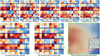 |
Fig. 4 ERO zodiacal light flat-field. This is a combination of large scales (>10ʺ) derived solely from the zodiacal light observed in any long VIS exposures and small scales (<10ʺ) coming from a weighted average of five high-S/N LED internal calibration images. These have wavelengths of 573 nm, 610 nm, 660 nm, 720 nm, and 890 nm, matching spectral coverage of VIS. The colour scale is arbitrary, set to explore the full range of intensity within each image. The top five images show the wavelength-dependent evolution of {gain × quantum efficiency}. This large-scale pattern is removed in the flat-field, replaced by the one from the pure zodiacal light image (bottom left). The overall left-to-right gradient is caused by the telescopic off-axis illumination and the VIS shutter effect (see also Euclid Collaboration: Cropper et al. 2025). The final ERO VIS zodiacal flat-field (bottom centre) incorporates all scales present in the Euclid signal, from pixel-to-pixel sensitivity variations (bottom right, highlighting a quadrant covering 205ʺ × 206ʺ, with a zoom on a 30 by 30 pixels area showing the pixel-to-pixel sensitivity differences) to the scale of the FoV. |
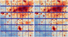 |
Fig. 5 Left: detrended VIS image of the Perseus cluster. This image follows the ERO mask, overscan, bias, flat-field, and deepCR corrections revealing a checkerboard pattern in a small number of quadrants, which is noticeable through the subtle relative jumps of the background level between adjacent quadrants. The effect is 2% of the background for the two most affected quadrants (if left uncorrected this would leave residuals at the 27 to 28th mag arcsec−2 level). Right: final image after applying a low-flux nonlinearity correction to approximately 30 quadrants. The image now displays uniform flatness of the background across all borders – both between detectors and within quadrants – indicating reliable photometry for extended emission such as galaxy stellar halos, intra-cluster light, and Galactic cirrus, as showcased here. The limiting surface brightness of these single frames exceeds 29 mag arcsec−2 throughout the entire FoV (direct detection of faint contrasts at the 10ʺ scale). |
4.2.6 Detector-to-detector image scaling
A VIS image, once corrected for additive instrumental components through overscan and bias corrections, and for multiplicative instrumental components with the main flat-field, results in an image that is uniformly flat. We anticipated a precise continuity of the background level across all borders, both detector-to-detector and quadrant-to-quadrant. However, during the processing of the 17 ERO fields, we observed that an additional step was necessary to adjust a few quadrants for a low-level flux nonlinearity caused by the analog-to-digital converter (ADC) chips in the readout electronics, some of which exhibit differential non-linearity (DNL), leading to irregularities in the voltage step amplitude corresponding to each bit. The left panel of Fig. 5 illustrates that some quadrants across the VIS mosaic appear either brighter or fainter than expected, leading to a residual checkerboard pattern that required correction.
As previously discussed, the zodiacal-light component in the ERO flat-field stems from observations of the south Galactic cap, where the zodiacal-light intensity is near its minimum, registering 29.7 ADU in our standard 566 s exposures. Conversely, the zodiacal background in most ERO fields is around 40 ADU. An investigation into this effect, utilising images with shorter integration times (and thus a lower total background in ADU), revealed that this discrepancy is purely multiplicative, scaling with the background flux. On average, only 30 to 40 quadrants, out of a total of 144 quadrants, required adjustment on a perERO project basis. This adjustment is necessary because the absolute zodiacal-light level varies from field to field. However, the correction factor for specific quadrants remained consistent across all fields. The average flux scaling needed was about 1%, with a maximum of 2% for the two most affected quadrants (if left uncorrected this would leave residuals at the 27 to 28th mag arcsec−2 level). This correction was implemented through a single multiplicative factor per quadrant derived visually. This is a first-order correction at the percent level, and it enables the first ERO science effort (some slight residuals can still be perceived after correction). The next ERO data release will include an automated recipe based on optimisation of gradients across all quadrant borders and mosaic gaps.
This ultimate multiplicative adjustment applied to the VIS images ensured that the continuity of extended emission was perfectly preserved (Fig. 5, right). However, this highlights the limitation of the ERO photometry to an accuracy within a few percent.
4.2.7 Quantisation noise
Upon analysing the noise characteristics of VIS images processed via the ERO pipeline, it was evident that the signature of quantisation noise from the analogue-to-digital converter (ADC) was present across all quadrants. This phenomenon, already noticeable in the raw data, persisted through detrending processes. Quantisation noise emerges from the rounding differences between the analogue input voltage to the ADC and its resulting digital output, an effect distinctly visible in a histogram of pixel intensity (Fig. 6, top). This noise is nonlinear and varies depending on the signal being converted.
It is important to recognise that the majority of Euclid’s scientific endeavours in the forthcoming years will focus on faint objects with relatively low S/N, meaning these objects will be faint sources superimposed on the image background. Such sources typically lie just to the right of the peak in the histogram of Fig. 6 (top), where quantisation noise is especially pronounced. This contributes to the photometric error budget, which remains primarily influenced by photon noise from the zodiacal light background, as well as readout noise. After resampling the image for stacking (Fig. 6, bottom), where neighbouring pixels are correlated, the effect of quantisation noise naturally diminishes.
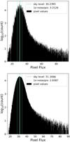 |
Fig. 6 Top panel: histogram of all pixels across a 200 arcsec2 region from a VIS detrended image. The histogram shows regular spikes at the 1 ADU frequency, indicative of quantisation noise (this effect is also observed in the raw data). Bottom panel: same region after resampling the detrended image with SWarp using a Lanczos3 function. The histogram shows that the pixels have been correlated and the quantisation error has been smoothed out. |
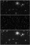 |
Fig. 7 Identification and removal procedure of the CR contamination. Images showing that the Python-based machine learning-driven tool deepCR effectively identifies (centre) and repairs (bottom) pixels affected by CRs (top). Each image segment (single rectangle) measures 2ʹ × 1ʹ, demonstrating deepCR’s effectiveness in enhancing image quality. |
4.2.8 Identification and removal of cosmic rays
Situated at the Earth-Sun Lagrangian point L2, Euclid is continuously bombarded by CRs of extragalactic, Galactic, and Solar origin. The CCDs’ deep-depleted silicon layer, 40 μm thick and designed for enhanced red sensitivity, is particularly susceptible to interactions with CRs (Fig. 7). Combined with the long VIS integration times, this results in raw images that are heavily contaminated: each 566-second-long image over the 0.52 deg2 FoV has approximately 1.4×10⁶ affected pixels. The prevalence of these transients impacts nearly all astronomical sources in the image and initially hindered our efforts to achieve a precise astrometric solution. Consequently, a method for repairing the affected pixels was explored and evaluated for widespread application in the ERO pipeline.
CR hits in individual images were identified and corrected using deepCR, a deep-learning-based CR removal tool specifically designed for astronomical images (Zhang & Bloom 2020). deepCR was developed and trained with images from the Hubble Space Telescope (HST) Advanced Camera for Surveys (ACS) using the F814W filter. Given the similarities in environment and detector characteristics between ACS and VIS, the deepCR model demonstrated remarkable efficiency in processing VIS images. Compared to other well-known methods such as LAcosmic (van Dokkum 2001), deepCR not only offers superior performance in both detecting and replacing affected pixels (by utilising in-painting rather than interpolation), but also operates relatively quickly on hardware equipped with a graphics processing unit. For instance, processing an entire VIS frame, including its 144 quadrants, takes about 50 s on an NVIDIA RTX 6000 Ada graphics card.
To evaluate the impact of the deepCR correction on final photometry, we conducted a set of tests. We added synthetic Gaussian profiles with a full width at half maximum (FWHM) corresponding to that of VIS images and fluxes ranging from 5000 to 500 000 ADU (as an integrated flux, meaning the sum of all pixels within 25-pixel apertures) to real VIS exposures impacted by CR hits. These modified exposures were then processed with deepCR. Following this, we performed source detection and photometric measurements on the corrected images using SourceExtractor (Bertin & Arnouts 1996), employing a conservative 25-pixel aperture diameter for analysis (noting that smaller aperture photometry, such as PSF photometry, would be even less affected). We find that about 20% of the artificial stars are unaffected by CR hits within the 25-pixel aperture and that the largest fraction of pixels affected within these apertures reaches approximately 10%. The comparison of output to input instrumental magnitudes for the sources affected by CR is depicted in Fig. 8, with the colour scale indicating the fraction of pixels within the 25-pixel diameter aperture affected by CRs as identified by deepCR. On average, the effect on magnitude is minimal, showcasing a skewed distribution with a mode around 1 mmag as well as 25% and 75% quartiles at 0.2 and 6 mmag. This negligible impact occurs almost independently of the number of pixels affected by CRs in the aperture, demonstrating the in-painting’s robustness and efficiency.
The approach we used not only maximises Euclid’s capabilities for astrometry but also enhances the cleanliness of the images for subsequent steps in the pipeline. Specifically, deepCR ensures that even with the standard ROS consisting of four dithered exposures, the resulting image stack is completely free of blacked-out pixels (out of approximately 606 million pixels) across the FoV due to CR contamination. This is particularly noteworthy because small areas of the FoV are exposed only once throughout the four-exposure dither, highlighting the role of deepCR in maintaining image integrity.
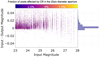 |
Fig. 8 Impact of deepCR corrections on photometric accuracy. Magnitude difference between the input synthetic stars and their measured photometry after applying deepCR masking and in-painting plotted against the input magnitude (using an arbitrary zero point). The colour scale on the graph represents the number of pixels within a 25-pixel aperture diameter that were affected by CRs. On the right side of the graph, a histogram displays the distribution of the magnitude differences, providing a visual representation of the photometric accuracy and the impact of CR corrections across various levels of CR contamination. |
4.3 Detrending NIR data from the NISP instrument
NISP uses 16 Teledyne H2RGs detectors of 2048 × 2048 pixels, arranged in a 4×4 mosaic with a plate-scale of 0ʺ.3 pixel−1. Extensive details about NISP are given in Euclid Collaboration: Schirmer et al. (2025). Similar to the procedures outlined for VIS, this section details the processing steps for NISP as they occur sequentially within the ERO pipeline, beginning with the correction of purely additive components of the instrumental signature.
4.3.1 Charge-persistence correction
Charge persistence is the process of trapping charge carriers within lattice defects of pixels and their slow release with a rate R during subsequent exposures. The effect is well-known, complex, and highly individual for H2RGs. For further details see for example Smith et al. (2008), Leisenring et al. (2016), Tulloch (2018), and – specifically for NISP – Kubik et al. (2024).
Persistence manifests as a faint version of previous images contaminating the following images. Strongly saturated pixels remain bright for many hours, resulting in complex persistence patterns from the preceding imaging and slitless spectroscopic exposures taken as part of the ROS (Euclid Collaboration: Mellier et al. 2025). Because masking the persistence would affect many pixels, we decided instead to model and subtract the persistence signal from each single exposure.
Ideally,  is measured using a bright LED flat image and a subsequent long series of dark images (Serra et al. 2015). Such data were taken during the PV phase in September 2023. The series was repeated three times with almost identical results. Therefore, we took the median of all three series to remove CRs. The persistence model was then derived from these median images.
We calculated  from the signal in each dark image at pixel (x, y), minus the bias pedestal of 1024 ADU, and normalised by the integration time and initial signal in the flat image (S ≈ 40 000 ADU). The measurements are shown in Fig. 9. To reduce the noise, we took the median value around each pixel in the interval [x − 2 : x + 2, y − 2 : y + 2]. Similar to the situation in CCDs (e.g. Kluge 2020), we find that
  follows a power law,
![${\log _{10}}\left( {\dot R(x,y,t)\left[ {{\rm{ADU}}{{\rm{s}}^{ - 1}}} \right]} \right) = A(x,y){\log _{10}}(t[{\rm{s}}]) + B(x,y).$](/articles/aa/full_html/2025/05/aa50803-24/aa50803-24-eq4.png) (1)
(1)
The slope A and offset B are fit for each pixel. An example for detector 1 is shown in the left two panels of Fig. 10. We notice strong spatial variations and an anti-correlation between A and B that cannot be explained purely by fitting uncertainties. The anti-correlation implies that the persistence signal is more stable than A and B individually.
The persistence signal P(x, y, tstart, tend) was then estimated by integrating R from the start tstart to the end tend of the subsequent exposures. We did not find any dependence of A and B on the initial signal S . Therefore, we simply scaled the predicted persistence by S:
 (2)
(2)
For a typical overhead of 60 s and integration time of tend − tstart = 87 s (effective exposure time from the entire duration of 112 s), we get P ≈ 0.0011 S to 0.0033 S, that is, a few per mille of the previous signal remain in the next image. This model is limited to unsaturated pixels. When saturation occurs, the true S value is unknown and cannot be estimated. However, masking those pixels with S > 50 000 ADU for 24 hours would result in too many mildly affected pixels being discarded, inevitably leading to some areas across the stack of four images with no signal. In the ERO pipeline implementation we left these pixels untouched and relied on sigma-clipping iterative algorithms to reject pixels affected by this specific persistence regime.
Complications arise because Ṙ varies over long periods of time. We suspect that the cause is related to the small-scale pattern in the dark images that is also visible in Fig. 10. The stripe pattern resembles spectra. Probably, saturation in a pixel affects the parameters A and B for longer time scales, an effect that has been observed in NISP ground tests and also in other H2RGs (see e.g. McLeod & Smith 2016). The true Ṙ can deviate by a factor of around 2 or more from the model prediction. We mitigate this effect by empirically rescaling P as Pʹ = P × K on a 10 × 10 grid (X, Y) for each detector (see Fig. 10, right panel). We refer to the elements of this grid as ‘blocks’. For each sufficiently large contaminated region i, we calculated the clipped median flux before subtraction Fin,org, and after subtraction Fin,sub, as well as outside of it Fout . The local correction is then
 (3)
(3)
This matches the flux inside the region to the surrounding flux. Corrections for single regions can be strongly affected by outliers. To increase the robustness, we take the median correction K(X, Y) = med[Ki(X, Y)] within each block. Because corrections are calculated for each single exposure and we do not observe strong short-term variations in K between exposures, we then combined all K for each day and ERO project by taking the median. The result is shown in the right panel of Fig. 10. The matrix K(X, Y) is then linearly interpolated on the finer grid K(x, y) to obtain a correction for each NISP pixel. The mean correction is mean(K) = 1.32 with a standard deviation of std(K) = 0.26.
For all spectra and images taken up to 1 hour prior to the current exposure, we modelled and subtracted the predicted persistence. First, we subtracted the clipped median signal from each preceding exposure before modelling its persistence. Although this is not correct in principle (because the background also creates persistence), this step is important to not deform the background signal due to imperfect estimations of Ṙ (x, y). We have visually verified that the effect on the predicted persistence is negligible. We only modelled persistence P < 70 ADU. For brighter persistence, we relied on outlier rejection using sigma clipping during the stacking procedure because modelling uncertainties would leave visible residuals. Masking these pixels could be beneficial, but we decided against it to avoid having empty pixels in the stacks. Consequently, the inner regions of bright objects can still contain persistence from previous spectra.
Figure 11, left panel, shows a region in the stacked Perseus ERO project that is strongly affected by persistence. The image in the right panel shows the result after successfully subtracting the predicted persistence from the single exposures. The diagonal stripe pattern that arose from the spectra taken just before the JE-band images is mostly gone. The effect on point-source photometry is P'/S ≈ 0.15–0.45%. More affected are the colour profiles of extended galaxies. The persistence from the spectra on the subsequently taken JE-band images makes the surfacebrightness profile locally brighter by approximately 0.05 mag. Overall, we estimate from our models that 2% (8%, 30%) of the area in the Perseus ERO JE-band stack was affected by persistence brighter than 25 (26, 27) mag arcsec−2 before our correction was applied. This highlights the importance of correcting for persistence in the NISP data.
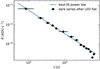 |
Fig. 9 Release rate Ṙ for an example pixel derived from an LED flat with a subsequent series of dark exposures. The data points show the persistence signal P in the dark images with the bias pedestal (1024 ADU) subtracted and normalised by the exposure time and initial signal S . The horizontal error bars mark the beginning and end of each dark exposure. The best-fit power law (A = −1.215, B = −1.829) is shown in blue. |
4.3.2 Bad pixel mask
The 16 H2RGs in NISP are of exceptional quality, featuring technology distinct from and not directly comparable to that of CCDs. Such detectors invariably have a higher fraction of pixels with marginal response. In applying the same approach as used for the VIS instrument – flagging nonlinear pixels through the analysis of the ratio of two internal LED illumination images – a significantly higher threshold of 10% (versus 1.2% for VIS) is required to avoid excessively flagging pixels. Below this threshold, pixels are corrected at first order by flat-fielding. Compared to VIS, the NISP mosaic exhibits significantly larger gaps between detectors, and with most ERO projects only involving four exposures per dither, overly aggressive flagging would result in numerous gaps in the final image stack, especially in the areas close to the mosaic gaps. The threshold was therefore adjusted upwards until all single ROS observations for ERO projects (comprising four exposures per NISP band) resulted in a stack with no sky pixels left unexposed.
Each detector in the NISP instrument consists of a 2040 × 2040 pixel array sensitive to light, with a total of 0.4% of pixels being masked. This proportion is comparable to that of the VIS instrument, despite a much higher threshold for identifying nonlinear pixels in NISP and a smaller total number of pixels (67 million for NISP). The distribution of masked pixels is consistent throughout the mosaic, with the notable exception of the top-right corner detector (DET16) that exhibits a 40% excess of masked pixels. The outermost four pixels around the periphery of the NISP H2RGs are insensitive to light. They are used for detector monitoring, do not significantly improve the ERO pipeline processing, and are thus simply masked.
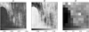 |
Fig. 10 Persistence model parameters for NISP detector 1. The parameters A and B are defined in Eq. (1). The correction factor K is shown for the date 2023-09-16. It is defined in Eq. (3). |
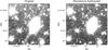 |
Fig. 11 Example region in the Perseus ERO JE-band stack before (left) and after (right) subtracting the predicted persistence from the single exposures. White corresponds to a surface brightness of approximately 25 mag arcsec−2. |
4.3.3 Electronic pedestal correction
Due to the onboard multi-frame sampling and subtraction performed before transmitting NISP images to Earth (for details see Euclid Collaboration: Schirmer et al. 2025), the pedestal of all raw NISP data is internally set to 1024 ADU. Subtraction of this value is hardcoded into the ERO pipeline. We observed a low-level time-dependent variation in the relative background level between detectors on a per-exposure basis. This leads to occasional mid- to large-scale background inhomogeneities in the final image stacks at the sub-percent level of the main background.
4.3.4 Dark current correction
Operating at a temperature of 95 K, the NISP detectors exhibit a low dark current, averaging 0.8 ADU per pixel over the duration of science exposures (112 s, leading to an effective integration time of 87.2 s). The dark current distribution across the detectors’ surfaces is highly structured (Fig. 12), necessitating the subtraction of a dark frame from the science images. NISP darks are obtained by inserting the dark plate mounted in the filter wheel (Euclid Collaboration: Schirmer et al. 2025). The master dark frame for the ERO data was generated using a median stack of 100 dark frames, each with an integration time matching that of the science exposures. These dark frames were captured following a prolonged period without any exposure to illumination, from astronomical sources or LEDs, to prevent any residual signal contamination due to image persistence.
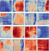 |
Fig. 12 Dark current map for the 16 NISP detectors. The final map is derived from a stack of 110-s integration dark frames that match the duration of the science exposures. The amplitude of the dark current varies, reaching up to 1.6 ADU at most across a single detector and with an average value of 0.8 ADU across the entire mosaic. The minimum in dark blue is 0.0 ADU; the maximum in deep red is 2.6 ADU. |
4.3.5 Flat-field correction for large and small scales
The NISP uses the same flat-field approach as VIS, combining zodiacal light and LEDs to correct image variations. This section highlights the differences between the two instruments, focusing on how we used light sources and on the adjusted processing methods for NISP’s NIR detectors compared to VIS’s optical detectors.
The sky background in the NISP bands is roughly the same as in VIS, about 22.3 mag arcsec−2, but a NISP pixel covers 9 times the area of a VIS pixel (0ʺ.3 versus 0ʺ.1 per pixel). Additionally, the single exposure integration time for NISP is about 1/5th of that for VIS. As a result, the zodiacal light signal per pixel is stronger in NISP, around 60 ADU in total per exposure. The associated photon noise (approximately 11 electrons) surpasses the readout noise (3.1 ADU, equivalent to 6.2 electrons), providing robust statistics for analysing the zodiacal light background and instrument-induced structures.
For creating the NISP zodiacal light flat-field, we selected a reference field free of extended sources located at the north ecliptic pole, featuring far fewer stars than the south ecliptic pole field adopted for VIS nearly on the line of sight of the Large Magellanic Cloud (stellar density was less in the IE-band, while the VIS resolution kept the footprint of stars limited). This choice was based on nearly 100 dithered frames captured over three days in early September 2023, with the same integration time as that used for the ERO programme. Despite its proximity to the Galactic plane, as outlined in the mission plan (Euclid Collaboration: Scaramella et al. 2022), this area is one of the three Euclid Deep Fields and is notably free from strong Galactic cirrus emission. The compilation of exposures from many different pointings ensures that the median stack effectively eliminates any isolated contamination.
For NISP, each photometric band is matched to a specific LED, as illustrated in Fig. 13. Detailed examination of these high-S/N frames across the three bands revealed the necessity to include significantly larger physical scales in the final flat-field than is done for VIS, due to the existence of distinct features that span hundreds of pixels. Capturing these extended structures at high S/N was crucial for achieving effective flat-fielding. Consequently, the crossover physical scale selected for NISP between the LED flat-field and the pure zodiacal light flat-field is 80ʺ. Adjustment of this scale was approached with precision to avoid artificial amplification of any structure that could be present in both input elements. This was achieved by flat-fielding the input images from the Deep Field North and meticulously examining their uniformity in the most sensitive areas of the NISP mosaic. The final ERO NISP flat-field is normalised to the average mode across all 16 detectors, resulting in detrended images that maintain characteristics similar to those of the raw data.
4.3.6 Row correlated noise correction
Upon visual inspection of the processed images, a faint residual noise is observed, exhibiting correlation across entire rows with variations around a single ADU (measured RMS of 0.7 ADU). This detector phenomenon can be modelled and subtracted by building a median of all rows. To avoid affecting extended emission, structures beyond a 15-pixel scale are first removed from the resulting vector before subtraction from each column of the image. This correction is illustrated in Fig. 14. While the fundamental noise properties remain unchanged, the data appear cleaner after correction.
4.3.7 High-fluence nonlinearity
The NISP H2RG sensors exhibit nonlinearity at high fluences, a characteristic whose details are unique to each pixel. Their full-well capacity is about 100 000 electrons, equivalent to 50 000 ADU given NISP’s average gain of two electrons per ADU. Nonlinearity typically becomes noticeable around 60 000 electrons, corresponding to 30 000 ADU for NISP. Since ERO science primarily deals with faint sources within the first few thousand ADUs, high-fluence nonlinearity is generally negligible. However, caution is warranted when measuring high fluences above 30 000 ADU, such as during photometric calibration using 2MASS (Cutri et al. 2003) stars.
There are also low-fluence nonlinearities, particularly from charge-persistence effects that we correct for empirically (Sect. 4.3.1), and from count-rate nonlinearity (Biesiadzinski et al. 2011) that is related to persistence and not explicitly corrected for by the ERO pipeline.
4.3.8 Inter-pixel capacitance
H2RG detectors exhibit inter-pixel capacitance (Le Graët et al. 2022) resulting in charge transfer or ‘cross-talk’ from the pixel where the charge initially accumulates to neighbouring pixels. This phenomenon increases the footprint of CRs and hot pixels across a larger area of the image, and also the core of the PSF, and can be considered another source of nonlinearity. However, since ERO science primarily utilises NISP as a photometer (with apertures covering multiple pixels to measure the flux of galaxies and stars), we ignore this effect. Nonetheless, it does contribute to the overall photometry error budget.
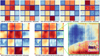 |
Fig. 13 ERO NISP zodiacal light flat-field. This combines the large scales (>80ʺ) derived solely from zodiacal light observed in any NISP exposures with the small and medium scales (<80ʺ) coming from specific LED internal calibration images tailored to each NISP band (only three LEDs were relevant for this purpose: 1160 nm, 1470 nm, and 1720 nm for YE, JE, HE, respectively). The arbitrary colour scale is used to fully explore the intensity range within each image. The top row displays the evolution of {gain × quantum efficiency} across all 16 NISP detectors at specific wavelengths, highlighting a large-scale pattern that is, however, omitted in the final flat-field in preference to the pattern emanating from the zodiacal light image (bottom left). The completed ERO NISP zodiacal flat-field (bottom centre, for HE) encapsulates all scales present in the Euclid signal, ranging from pixel-to-pixel sensitivity variations and low-to-medium-sized features (bottom right, showing a detector of 612ʺ × 612ʺ, with a zoom on a 30 by 30 pixels area showing the pixel-to-pixel sensitivity differences), extending to the entire FoV scale. The relative colour range from dark blue to deep red is an intensity ratio of 12% on average across the full mosaic panels and 5% for the variations across the single detector on the lower right. |
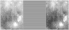 |
Fig. 14 Left: original image (900 px× 1200 px area of a single NISP detector). Horizontal striping indicative of row-correlated noise is easily noticeable. Middle: noise model constructed spanning the image’s width to specifically target and quantify the noise pattern. Right: corrected frame where the row-correlated noise has been mitigated. This image demonstrates that the procedure effectively addresses the noise issue without substantially impacting the extended emission in the image. The residual image persistence caused by the NISP spectra generates an apparent column-correlated noise. |
4.3.9 Cosmic rays
We were unable to implement a robust CR identification solution for NISP in time for this data release. With a pixel sampling of 0ʺ.3 leading to an FWHM of 1.6 pixels, distinguishing CRs from stars becomes challenging because they often appear similar. Tools such as deepCR, effective for VIS data, are not suitable, due to inadequate training.
Due to bandwidth limitations, individual frames taken as part of the NISP exposure ramps (Euclid Collaboration: Schirmer et al. 2025) cannot be downlinked to Earth, and an onboard slope fit is performed instead to estimate the accumulated signal in a pixel. The fitting procedure provides a flag indicating whether an individual pixel was hit by a CR during the exposure (see Kubik et al. 2016, for details). Applying this flag mask would lead to the discarding of an excessive number of pixels for the ERO observations, a problem reminiscent of the issue encountered with the bad-pixel mask versus sky coverage. As a result, we did not correct or flag CRs and instead relied on iterative sigmaclipping methods to reject them when generating the science stacks.
For ERO data employing a single ROS with only four dithered exposures per band (see Table A.1), a fraction of the FoV situated at the intersection of the gaps between four detectors – totalling nine areas within the main area of nominal S/N – receives astronomical signal only once. Consequently, these nine small rectangular areas still contain residual CRs in the final stacks. However, by combining information from other Euclid bands at the catalogue level, we can flag and reject these residual transients. Since they are unlikely to affect all four single visits on the sky across the three NIR bands, this is achieved through the utilisation of a Χ2 detection image (see Sect. 8).
5 Astrometric calibration
5.1 Initial astrometric solution
In the context of processing the ERO images for integration into the pipeline, we noted that the raw FITS headers only provide the central coordinates of the observed fields. To establish a refined astrometric framework, a crucial initial step involved anchoring a minimum of one quadrant for VIS or one detector for NISP to the WCS. This key task was accomplished through the deployment of Astrometry.net, operating in a local environment and utilising the most comprehensive index derived from Gaia-DR3.
Advancing to the subsequent stage that entails the construction of global mosaic astrometry for both VIS and NISP instruments, the process is notably facilitated by the preliminary calibration of all quadrants or detectors via Astrometry.net. In this vein, custom catalogues were generated for certain ERO fields where stellar density was compromised, attributable to factors such as high Galactic latitudes (for instance, the Fornax field) or significant attenuation, such as in Messier 78. The catalogues were sourced from the Dark Energy Survey Instrument Legacy Imaging Surveys (Dey et al. 2019) and the Unwise Catalogue (Schlafly et al. 2019), and were tuned for the small angular scale of Euclid VIS quadrants by selecting quadrangles of stars with scales a factor of  and 2 smaller than the standard Gaia-based catalogues.
5.2 Global image astrometry
Astrometric calibration was performed using an enhanced version (V2.13) of SCAMP (Bertin 2006), utilising catalogues generated from processed images initially calibrated with Astrometry.net. In essence, SCAMP calculates a global astrometric solution by minimising, in the least-square sense, the mutual differences of the reconstructed source positions in all overlapping exposures, plus the differences in position with respect to an arbitrary reference catalogue. The reference catalogue employed for calibrating ERO data is Gaia-DR3 (Gaia Collaboration 2023).
In SCAMP, geometric distortions represent deviations from a fiducial projection that is assumed to be tangential (gnomonic). At any position in the focal plane, SCAMP models the geometric distortions for a given instrument and filter as the sum of two polynomials: a chip-dependent constant polynomial; and a mosaic-wide, exposure-dependent polynomial of low degree. The VIS and NISP focal planes exhibit minimal geometric distortions; we adopted a third-degree polynomial for the chipdependent component and a first-degree polynomial for the exposure-dependent component, since we found them sufficient to calibrate astrometry to the milliarcsecond level. VIS and NISP were calibrated separately, because no gain in precision was achieved with a combined astrometric run, with the relatively coarse sampling of NISP remaining the limiting factor.
A considerable limitation of SCAMP is its inability to directly incorporate proper motions within the calibration process. As a result, for observation and reference data sets spanning different epochs, the calibrated coordinates must be adjusted in a subsequent step (Bouy et al. 2013). ERO exposures are captured within a brief period, thereby sharing a common epoch, tERO = 2023.7. However, there is a substantial temporal gap when compared to the Gaia-DR3 epoch, tDR3 = 2016.0. SCAMP corrects for the proper motion vector μ*DR3 of each reference Gaia star by actualising its celestial coordinates using
 (4)
(4)

is a Tikhonov regularisation factor that accounts for possibly large proper motion uncertainties; in practice κ remains very close to 1 for a large majority of stars.
Although the ERO projects were all conducted nearly perpendicular to the antisolar direction, we neglected the effect of parallax between the Gaia and Euclid observations that is below the milliarcsecond level for the vast majority of stars used in the calibration. For simplicity, we also ignored correlations between the positional errors in right ascension and declination, as well as between positions and proper motions in the Gaia sample. The final positional uncertainties corrected in the astrometric reference sample are determined by adding in quadrature the proper motion uncertainties, scaled by the time difference. A significant portion of the Gaia-DR3 catalogue entries lack proper motion measurements; rather than discarding these entries outright, we found that it enhances the robustness of the solution for SCAMP to assign zero proper motions to these stars, with an arbitrary proper motion uncertainty of 10 mas year−1 in both axes. Fig. 15 shows an example of astrometric residuals for the challenging NGC 6397 ERO field (Massari et al. 2025), where most globular cluster stars lack proper motion estimates in Gaia-DR3.
Overall for VIS, the median internal astrometric precision (dispersion among calibrated coordinates) for sources with an S/N > 100 is 6 mas RMS across the 17 ERO fields in both axes. This figure accounts for contributions from compact, yet resolved sources; when the selection is limited to point sources, the median internal dispersion decreases to 2 mas RMS. Additionally, the median external accuracy, defined as the RMS dispersion of the difference between the averaged calibrated coordinates over all overlapping exposures and the corrected Gaia-DR3 coordinates, is 8 mas RMS. In comparison, the performance metrics for NISP are 15 mas RMS for internal precision and 10 mas RMS for external accuracy, respectively. The astrometric performance of both VIS and NISP indicates that images are calibrated to a precision of 1/15th of a pixel across the entire FoV.
6 Resampling and stacking
Image resampling and stacking represents a classic method for combining individual exposures onto a common pixel grid. Resampling affects VIS and NISP exposures, both of which are significantly undersampled – NISP even more so – potentially leading to image smoothing and/or aliasing artefacts. A non-destructive alternative for merging multiple observations is to conduct simultaneous measurements across all overlapping exposures, each on its own pixel grid (Bertin et al. 2020). However, this method entails slower processing, yields larger and more complex end products, and complicates the handling of residual glitches.
Therefore, in the context of the initial Euclid science efforts with the ERO programme, we opted to adhere to the conventional method of resampling and stacking. The SWarp software package (Bertin et al. 2002), is at the root of the two flavours of ERO stacks that we use (Fig. 16), as now described.
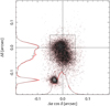 |
Fig. 15 Post-calibration astrometric residuals along the RA and Dec axes for unsaturated Gaia-DR3 stars in the NGC 6397 field (Massari et al. 2025). Residuals were computed for each star as the difference between the calibrated coordinates on the individual VIS exposures and the corrected Gaia-DR3 coordinates (see text). Grey points represent a subsample of detections with a S/N > 100 on ERO exposures. The plot reveals two distinct groups of stars, represented as a large cloud slightly offset from the centre and a small compact cloud clearly separated from the centre, both consisting of stars lacking proper motion data in the DR3 catalogue. The position offset of the smaller ‘cloud’, located in the lower left, aligns well with previous estimates of the NGC 6397 absolute proper motion (μ* = (3.6,−17.3) mas yr−1, Kalirai et al. 2007), over a period of 7.7 years. A dashed square at the centre of the plot illustrates the size of the VIS pixel footprint for comparison. On this specific ERO field the internal astrometric precision is 2.7 mas RMS. |
6.1 The compact-sources stack
For the compact-sources stack we activated the background modelling and subtraction, removing extended emission signatures and thus yielding a background of zero ADU. We refer to this stack as the ‘ERO compact-sources stack’, optimised for the detection and photometry of compact sources.
We resampled and stacked the images in a single SWarp run, adopting a mesh size of 6ʺ , matched to both instruments – with BACK_SIZE set to 64 pixels for VIS and 22 pixels for NISP – to eliminate extended emission. This facilitates for example the detection of faint sources embedded in the halos of galaxies. We utilised the SWarp option for clipped-mean stacking (Gruen et al. 2014) to enhance the final S/N also excluding CRs in NISP and occasional CR residuals from the deepCR operation for VIS.
Prior of this step, a weight map was produced for each input image using WeightWatcher (Marmo & Bertin 2008), based on the bad-pixel mask and the flat-field used for detrending the raw data. SWarp compiles a weight map for the science stack from all input products, which is crucial for tracking the noise properties across the image and is a key element for source extraction (see Sect. 8 for the creation of the catalogues). SWarp also updates the average gain in the stack’s FITS header (GAIN) according to the weight map. For NISP, a Χ2 detection image (Szalay et al. 1999) is eventually generated by SWarp based on the three YE, JE , HE stacks.
6.2 The extended-emission stack
The extended-emission stack preserves extended emission (covering both high and low surface-brightness science) and is suited for both high and low surface-brightness objects. It is created by initially generating an individual SWarp-ed image from each input image, with the background subtraction option deactivated to retain all scales. The FSCALASTRO_TYPE option is set to NONE to ensure the preservation of the number of ADUs per pixel, which makes this stack inappropriate for the study of compact sources.
Despite minimal variations from one exposure to the next, the true zodiacal background for each image is measured through an optimisation step to a precision of 0.01 ADU to facilitate piston correction during stacking (the background is steady at the sub-ADU level from exposure to exposure due to the stable environment). This is achieved using a dedicated CFHT-MegaCam Elixir-LSB pipeline with a sigma-clipped mean function, developed for the Next Generation Virgo Survey (Ferrarese et al. 2012). The median value of the background levels from the input images is reintegrated into the final extended-emission science stack, aiding in the tracking of noise properties. Sigma-clipping is set to be more stringent for NISP than VIS to eliminate residual persistence. The weight map produced by SWarp for the compact-sources stack serves as a proxy for the extended- emission stack, and the FITS GAIN keyword is duplicated from the compact-sources stack to maintain consistency.
6.3 Resampling
The resampling step included the adjustment of flux scaling to achieve our target photometric zero point (ZP), as outlined in the preceding section, utilising SWarp’s FSCALE_DEFAULT option. A crucial decision in this process is the selection of the interpolator. Given the low number of overlapping exposures (≤4), interpolating functions with support smaller than the destination pixel, such as those used by Drizzle (Fruchter & Hook 2002), are impractical here.
For VIS we opted for the Lanczos3 kernel as the interpolant so as to preserve sharpness as much as possible – a requirement driven by the ERO science – and to minimise correlations and moiré effects in the background noise. Through this process, the VIS FWHM changes from 0ʺ.136 in the unresampled image to 0ʺ.158 post-resampling and stacking, as measured by PSFex (Bertin 2011). The VIS channel is significantly undersampled, and the bandwidth-preserving quality of Lanczos3 interpolation is not immune to aliasing. Consequently, the precision of certain measurements on VIS image stacks, such as PSF fitting, may be compromised by aliasing in the brightest sources. However, in our tests we found that the slight improvement in resolution over other resampling methods – for example a bilinear kernel – in the resulting stacks outweighed the negative effect of aliasing residuals, making it a suitable compromise for ERO science.
For NISP images, employing Lanczos interpolation would lead to excessive artefacts due to the more pronounced undersampling and the prevalence of CRs predominantly affecting individual pixels. Consequently, we used bilinear interpolation instead. The NISP FWHM then varies from 0ʺ.42 to 0ʺ.49 on average across the YE, JE, and HE bands, as measured by PSFex.
The pixel-to-pixel correlations resulting from resampling affect the amplitude of the background noise measured by SourceExtractor. Utilising SkyMaker v4 simulations (Bertin 2009; Carassou 2017), we estimate that SourceExtractor underestimates the RMS amplitude of the background noise on larger scales by a factor of approximately 1.32 for the VIS channel and 1.69 for the NISP. This assessment is based on the assumption that the input readout and photon noise are perfectly white, and that an infinite number of images, uniformly distributed in position, contribute to the stack.
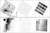 |
Fig. 16 Top: (left to right) ERO Perseus cluster in the HE-band (full FoV of 0.70 deg2) showing the extended emission stack, compact-sources stack, and weight map (all in inverted scale). Bottom (left to right): ERO Horsehead Nebula in the IE-band (full FoV of 0.59 deg2) showing the extended emission stack, compact-sources stack, and weight map (all in inverted scale). All ERO fields are rotated to deliver a standard equatorial projection where north is up and east is to the left. The main difference between the two types of stacks (center versus left) is the suppression of extended emission in the compact-sources stack to optimise compact source photometry. The two flavours of stacking are motivated by the need to optimise the photometry for each class of objects (it is not recommended to use the extended-emission stacks for compact-source science). The weight maps echo the observing strategy, with a S/N that can vary greatly across the image. This is particularly striking on the bottom right, based on a standard Euclid observing sequence. |
6.4 Co-addition
The culmination of stack processing that impacts the pixels involved creating a common-FoV mask for both the VIS and NISP instruments, retaining only pixels containing valid sky data in both stacks. Although VIS and NISP share a common FoV as shown on Fig. 17, the differing geometries of their detector mosaics and the size of the gaps result in distinct final stack outlines for each instrument. The binary mask aligns both instruments to a uniform standard. It is applied not only to the stacks but also to their respective weight maps.
The process does not attempt to create clean edges around the images; instead, the final outline is determined solely by the combination of the dithering pattern, the sky orientation from L2 at the time of observation, and the footprint of each mosaic. In the FITS files, masked pixels are assigned the value NaN. In the final stage of processing, crucial FITS keywords are adjusted to accurately reflect the characteristics of the data (e.g. SATURATE, GAIN), alongside other miscellaneous information such as the origin of the data, and details about the pipeline and its operation.
7 Photometric calibration
The initial flux calibration of the ERO data is based on pre-launch instrument and telescope parameters, and it is followed by validation against external catalogues. The pre-launch ZPs, denoted as ZP0 , are documented for NISP in Euclid Collaboration: Schirmer et al. (2022) and calculated similarly for VIS. Their respective values are 25.72, 25.04, 25.26, and 25.21 for IE, YE, JE, and HE, representing the AB magnitudes that correspond to a signal of 1 e− s−1, for a source with a frequencyflat SED. The ZPs in user-ready ERO data correspond to the AB magnitudes for 1 post-processing ADU. Their initial values depend on the gain yg and exposure time τ for each detector. For VIS, with a typical g = 3.5 electrons ADU−1 and an exposure time τ = 566 s, 1 initial ADU corresponds to a magnitude of 25.72 − 2.5 log10(g/τ) = 31.24. For the ERO pipeline we adopted an arbitrary ZP = 30 for all images at this stage; the pixel values were rescaled accordingly, with a corresponding adjustment of relevant image-header keywords such as the gain and saturation values.
The stacking procedure, which typically averages four images, has no effect on the ZP but does affect the effective gain. The gain is not constant over a stack, for instance because the number of input images available per output pixel varies as a result of gaps between detectors and masked pixels. An effective gain is computed by Swarp and stored in the image header. Swarp also provides a weight map that incorporates information on the number of images used at each pixel. For photometric measurements, SourceExtractor automatically adjusts the effective pixel gain using the input weight map (with WEIGHT_GAIN = Y, the default), assuming that the pixel gain scales with the weight.
The initial photometric calibration of the stacks was verified against external catalogues to adjust ZPs where necessary. The availability of external catalogues for this purpose varies depending on the observed area. The all-sky Gaia data are adequate for the validation of IE photometry (see Fig. 18). Additionally, data from the Dark Energy Survey (DES) were used (their DR2; Abbott et al. 2021), as well as Pan-STARRS 3pi Survey DR2 data from MAST (PS1; Chambers et al. 2016); individual ERO projects also made use of data from other surveys, as available. The process is illustrated below for the FoVs of ERO Dorado, which overlaps with DES and ERO Perseus, which overlaps with PS1.
The validation procedure involved comparing the magnitudes of non-saturated stars with those predicted from external catalogues, using transformations calculated from tables of synthetic stellar photometry. Initially, we identified the types of stars present within the relevant magnitude range along the line of sight towards the ERO field. This identification relied on the Besançon model of the Galaxy (Robin et al. 2003; Czekaj 2012; Lagarde et al. 2021)2, which also underpinned the pre-launch sky simulations by the Euclid Consortium (Euclid Collaboration: Serrano et al. 2024). VIS saturates near IE = 18.5 AB mag. For IE magnitudes between 18.5 and 24, main sequence stars overwhelmingly predominate. Stars near the turn-off, being intrinsically brighter, are generally found in this magnitude range when they reside far out in the halo, thus being metal-poor and α- enhanced; as we move to intrinsically redder and fainter stars along the main sequence, we encounter more disc dwarf stars with typically Solar metallicities and [α/Fe] ratios. This distribution was taken into account when selecting relevant stellar spectra for synthetic photometry, thus reducing the dispersion in synthetic colour-colour diagrams compared to combining stars of all types. The selection can also aid in calculating suitable colour-dependent extinction coefficients.
Two libraries of stellar SEDs were employed: (i) a collection based on the semi-empirical BaSeL 2.2 library by Lastennet et al. (2002), corresponding to the library described in Euclid Collaboration: Serrano et al. (2024); and (ii) a collection of theoretical stellar spectra generated with the Phoenix stellar atmosphere and radiative transfer code by Husser et al. (2013), previously utilised by Powalka et al. (2016) for a similar objective. These libraries are referred to as SSED and TSED, respectively, with only the latter allowing for an explicit consideration of the trend in [α/Fe]. The selection process is demonstrated for two ERO fields in Appendix C.
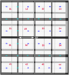 |
Fig. 17 Common FoV of VIS and NISP. This image was generated from two VIS and NISP images taken simultaneously with common astrometry applied. The small blue numbers refer to VIS, and the large red numbers refer to NISP detector IDs. The interchip gaps of each mosaic is evident. The VIS detectors show an additional thin horizontal gap from the charge-injection lines. The respective spatial and angular offsets between both instruments are 52ʺ.5 and 0°.078. Figure from Euclid Collaboration: Mellier et al. (2025). |
7.1 VIS photometric calibration
Gaia magnitudes are particularly well-suited for predicting IE magnitudes due to their accuracy and uniformity across the sky, as well as the low dependence of the theoretical transformation from Gaia passbands to IE on the adopted SED models. This compatibility is evident in Fig. 18 and in particular Fig. 19, where the synthetic photometry from both the semi-empirical and theoretical libraries shows good overlap across a wide range of colours3. Coincidentally the extinction vectors, which are colourdependent in the broad IE filter, are essentially tangent to the expected stellar locus in plots of IE − GGaia versus GBP − GRP at all relevant colours. The empirical data points in Fig. 19 were derived from IE aperture photometry in an aperture size of 4ʺ. 8 radius. According to our PSF models, this size encapsulates more than 98% of the light (Table 3). We corrected for the small missing fraction when needing to accurately express the true brightness of observed stars.
The Gaia data were acquired through a cross-match with Gaia-DR3 using the CDS4 cross-match tool (Boch et al. 2012; Pineau 2020) accessible via the Topcat software (Taylor 2005); the passbands for synthetic photometry were also based on Gaia-DR35. Gaia’s photometry was initially presented in the Vega magnitude system. Our conversion from Vega to AB magnitudes utilises the model Vega spectrum sourced from the SVO filter transmission service6 (Rodrigo et al. 2012; Rodrigo & Solano 2020) in September 20237.
The residuals observed vary with brightness and colour (Fig. 19). This comparison was extended across several ERO projects and we also employed PS1 as a reference in place of Gaia, yielding similar outcomes. Factors contributing to these discrepancies include nonlinearity within the VIS instrument, the PSF dependence on magnitude known as the brighter-fatter effect (Antilogus et al. 2014), possible changes of the in-flight passbands compared to pre-launch measurements, and the fact that flux calibration in broad filters inevitably has a colour dependence that a flat-field based on a single light source (zodiacal light in our case) cannot capture. Further analysis will be needed to disentangle the effects of brightness and colour in the ERO data and remove the residual trend. An average offset was calculated for ERO data using stars within the range of 18.5 ⩽ GGaia ⩽ 20 (after conversion to AB magnitudes), amounting to −0.13 mag, leading to the 30.13 ZP reported in all final VIS stack FITS headers. While the residuals for most ERO projects are centred around this value, some exhibit deviations as large as 0.05 mag.
To further investigate the observed discrepancy between observed IE and the prediction based on Gaia, as well as the dispersion in that comparison, we analysed the residuals by segregating them according to each detector in the VIS mosaic. Fig. 20 depicts such an analysis. The horizontal red line represents the average ZP offset for the entire mosaic. It is observed that the ZPs vary substantially across different detectors. An examination of the 16 individual images reveals that in some cases the ZP is not uniform even within a single detector. This variation is likely attributable to drift among the four amplifiers used in each detector. We further find a lack of uniformity from one image to the next, underscoring the complexity of achieving consistent photometric calibration across the mosaic. Calibrations and observations conducted during the PV phase (concurrent with the ERO observations) and described in Euclid Collaboration: Mellier et al. (2025) demonstrate that, with corrections in place for effects not considered here (including the brighter-fatter effect, optical ghosts, non-linearity, and the illumination correction), the Euclid surveys meet the relative photometric requirement of better than 1%.
Another factor contributing to spatial and temporal photometric variations is the contamination of optical surfaces with water ice from molecular outgassing (Euclid Collaboration: Schirmer et al. 2023). It is known that Euclid experiences outgassing effects in particular in the VIS optical path, resulting in time-variable throughput losses that may also be spatially variable. A thermal decontamination of the affected mirror was successfully undertaken in March 2024 to restore the transmission to immediate post-launch values. Directly calibrating VIS images taken at different times against Gaia removes at least the global flux-scale offsets.
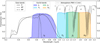 |
Fig. 18 Spectral response of Euclid’s wide imaging bands. For comparison we show the Gaia bands that we used – among others – for photometric calibration of the VIS IE-band, and the atmospheric transmission that limits the ground-based Y, J, H, and Ks bands, for a precipitable water vapour level of 1.0 mm from Rothman et al. (2013). Considerable colour terms may arise for individual sources when transforming fluxes in the wide Euclid bands to fluxes in other photometric systems. |
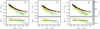 |
Fig. 19 Calibration of IE against Gaia. The upper panels display the colour transformation between Gaia-DR3 photometry (converted to the AB magnitude system) and IE for Milky-Way stars in the ERO fields towards Dorado (left panel), Perseus (middle), and NGC 2403 (right). In the lower sub-panels, the residual difference between the predicted and observed IE photometry is plotted. The coloured symbols represent observations, as determined from stacked images using photometry in a large aperture and the pre-launch ZP, that is a stack ZP of 30 as described in Sect. 7. An average foreground extinction is applied to the synthetic photometry, as adequate for each line of sight; the empirical data have not been dereddened. Two extinction vectors are shown in each figure, both for AV = 0.5, with one appropriate for the bluest stars and one for the reddest ones. Coincidentally the extinction vector is almost aligned with the colour-transformation curve at all colours; as a result extinction corrections of up to AV = 1 change IE,obs − IE,pred by less than 0.01 magnitude. |
Aperture–magnitude corrections for the ERO catalogues.
7.2 NISP photometric calibration
An initial evaluation of the fluxes from non-saturated NISP point sources was conducted using 2MASS photometry (Cutri et al. 2003), following the linear transformation equations detailed in appendix C of Euclid Collaboration: Schirmer et al. (2022). A limitation of this approach is the restricted dynamic range for comparison, spanning only about 1 magnitude. Specifically, the faintest sources in 2MASS approach the saturation limit in NISP. There is a broader overlap with more recent NIR surveys that reach depths between those of 2MASS and Euclid; these surveys typically base their calibration on 2MASS, offering a more extended range for comparison and potentially enhancing the accuracy of the NISP flux comparison.
The top row of Fig. 21 presents a comparison with photometry from the DES along the line of sight towards Dorado. Notably, for cool stars, significant discrepancies are seen between the synthetic photometry produced by different spectral libraries. The SSED library exhibits a problematic junction between the optical and NIR wavelength ranges, resulting in a step-like anomaly near 1 μm in some spectra. Conversely, the TSED library demonstrates more consistent behaviour; however, similar to other theoretical libraries, it does not perfectly align with empirical SEDs below approximately 4500 K, as noted by Lançon et al. (2021). Near the hook that appears in the empirical stellar sequence in some of the colour-colour diagrams, the TSED library shows that the expected behaviour depends strongly on metallicity and surface gravity, adding uncertainty unless detailed stellar parameters are exploited. Consequently, transformation equations between systems are derived from, and applied exclusively to warmer stars, where model-dependence is minimal. Extinction effects are included but negligible in these colour planes towards Dorado, compared to differences between models.
To determine if systematic uncertainties in DES colours (represented on the x-axis) contribute to the observed discrepancy between predicted and observed NISP magnitudes, comparisons were also made using (iDES − yDES) and (yDES − zDES). The residuals were consistent across these comparisons, and showed an offset of -0.05 in YE, and of approximately +0.1 in JE and HE.
The lower row of Fig. 21 considers the data of the Perseus ERO project, and provides a comparison between NISP photometry and PS1 data. In this region, extinction plays a more significant role with typical values around E(B − V) = 0.15 mag, exhibiting spatial variability by approximately a factor of 1.8 across the field (Marleau et al. 2025). Furthermore, the extinction varies with distance for stars within the Galactic disc. This contributes to dispersion but mostly at the red end of the stellar colour distribution, which we avoid in the calibration procedure. The most significant effect is seen for HE , where an increase of the adopted AV by 0.1 mag decreases the offset between predicted and observed IE by 0.011 mag. With AV = 3.1 E(B − V) = 0.45 mag, the average deviation between predicted and observed magnitudes in Perseus is negligible for YE, and approximately +0.1 mag for JE and HE. This analysis was supplemented with a consistency check using galaxy magnitudes, converted to HE from the 2MASS galaxy catalogue, yielding similar discrepancies. Because the average offset values were finalised after the images for first ERO datarelease were frozen for science production and distribution as part of the first ERO data release presented in this paper, the photometric zero points in those first-release NISP image FITS keywords are not updated8; we recommend to subtract 0.1 mag from the header ZPs of the JE and HE stacked images, and to subtract 0.1 mag to all JE and HE magnitudes in the ERO catalogues delivered with this first release. The next ERO public data release will integrate this adjustment. For consistency in the first ERO public data release, Table 2 summaries the data set’s general properties, listing the zero points as found in the FITS headers and adopted for catalogue production.
Overall, the derived ZPs align closely with pre-launch expectations, showing variations within approximately 0.1 mag across different ERO projects. Such variations are entirely plausible, considering that the ERO pipeline has not yet undergone nonlinearity calibration or photometric flat-fielding adjustments. Furthermore, the absolute quantum efficiency of the NISP detectors carries an uncertainty of about 5%, due to an entanglement with the detector gain (Waczynski et al. 2016; Secroun et al. 2018) among other factors. Finally, the definition of the total stellar flux, encoded in aperture corrections, may differ between surveys. Subsequent analysis of photometry in the three NISP bands within the ERO data framework did not uncover any significant inconsistencies in this calibration, staying within the broader uncertainties inherent to the ERO pipeline process.
In summary, the uncertainty of the absolute flux calibration of the VIS data after calibration against Gaia fluxes, is better than 1% on average, with residual trends versus colour and brightness with joint amplitude of the order of 10%. In NISP, the absolute calibration is limited to about 10% by the stronger model-dependence of the colour transformations to reference data, and a limited calibration set in the early months of observations.
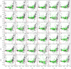 |
Fig. 20 Illustration of the IE magnitude offset with respect to pre-launch estimates of the ZP, per detector, using one exposure on the Perseus galaxy cluster. The horizontal line indicates the average offset, while the green symbols represent stars with a Gaia colour of (GBP – GRP) < 1.8. These stars were specifically used to calculate the average offset, highlighting the variations across different detectors and emphasising the impact of stellar colours on the observed magnitudes. |
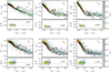 |
Fig. 21 Colour transformation between DES and Euclid NISP photometry for Dorado (top) and between PS1 and Euclid NISP photometry for Perseus (bottom). The figure setup is as in Fig. 19. Extinction is applied to the synthetic magnitudes (AV = 0.05 mag in the case of Dorado, AV = 0.45 mag in the case of Perseus), and a typical extinction vector for AV = 0.5 mag is also shown. |
General median properties of the 17 Euclid ERO fields with a 0.60 deg2 sky coverage for single ROS observations.
8 Compact source catalogues and general performance of the ERO data set
8.1 PSF modelling
For photometric analyses, a PSF model is essential for each image stack. The PSF model is computed using PSFEx (Bertin 2011) that employs a super-resolution algorithm along with a simple regularisation scheme to map the PSF at sub-pixel resolution. To minimise the contribution from spurious Nyquist modes, we choose a PSF sampling step of 0.45 pixels.
The Euclid PSF shows remarkable homogeneity across the FoV(Euclid Collaboration: Mellier et al. 2025), aligning with the stringent requirements set for the instrument. We find that for our purposes a second-degree polynomial adequately captures the PSF’s subtle variations across the entire image. As anticipated, the precision of the PSF models derived from the stacks is limited by aliasing and image resampling, with these effects being particularly pronounced in the NISP data.
Despite these challenges, the typical Χ2 per degree-of- freedom value for PSF models fitted on bright point sources in VIS stacks remains at a reasonable level of 1.7. However, for the NISP stacks, this value escalates to around 10, indicating a higher level of deviation from the ideal PSF model, primarily due to undersampling (see also Euclid Collaboration: Schirmer et al. 2025).
8.2 Production of the science validation catalogues
Rich photometric catalogues were produced using SourceExtractor on both the VIS and NISP compactsources stacks, utilising inputs such as PSFs derived by PSFex, the weight maps, the NISP Χ2 detection image created by SWarp, and the updated photometric ZPs as previously described. Source extraction for the VIS IE -band catalogue was performed in stand-alone mode, benefiting from its higher depth and resolution. The deep nominal detection image produced by combining the three NISP bands led to a uniform source extraction approach across all three bands and a consistent segmentation map from the three SourceExtractor runs for NISP for a given field. The ERO collection primarily includes 34 stacks and 17 weight maps and catalogues for VIS, together with 102 stacks and 51 weight maps and catalogues for NISP.
The ERO catalogues include model-fitting measurements (e.g. SourceExtractor’s MODEL / SPHEROID / DISK / POINTSOURCE), totalling 163 requested parameters, with several generating multiple columns in the photometric catalogue. Consequently, the ERO science-validation catalogues feature a total of 363 parameters per identified source. Table E.1 in Appendix E lists all input parameters along with their descriptions and units.
SourceExtractor was configured with a detection and analysis threshold of 1.5 σ, bringing a comprehensive census of compact sources (stars and galaxies) within the images. The internal background subtraction utilised a mesh size of 6ʺ.4, mirroring the precise setting employed by SWarp for the stacks. The catalogues provide a series of 10 aperture photometry measurements (MAG_APER). For VIS (0ʺ.1 pixel–1) the diameters of the apertures in pixels are 20, 3, 6, 12, 24, 48, 96, 58.5, and 80, spanning from the 2nd to the 10th aperture. For NISP, these pixel values are adjusted due to the different pixel scale of 0ʺ.3 pixel–1. The initial aperture should be disregarded because it was an exploratory measure based on FWHM that did not yield useful insights. The 9th and 10th apertures align with certain apertures used in the DES official products (5ʺ.8437, and 8ʺ). The magnitude offsets that must be applied to the catalogues for each aperture to obtain the total magnitude are detailed per Euclid band in Table 1, stemming from an analysis of encircled energy in the PSF discussed later in Sect. 9.2.
While individual ERO teams typically developed photometric catalogues tailored to their specific scientific objectives, a collaborative effort among the six teams resulted in the establishment of a general format designed primarily for compact-sources science. These catalogues are both comprehensive and versatile, facilitating a wide spectrum of scientific research. Accompanying the stack images, these catalogues represent a crucial component of the ERO public data release, enabling diverse astronomical studies.
These catalogues also served to assess the performance attained in each ERO field as outlined in Table B.2, leading to their designation as science-validation catalogues. To reproduce and verify the work, miscellaneous configuration files and derived data products from the AstrOmatic tools (PSFex, SourceExtractor) used to produce the components of the final catalogues are provided as well. Among these data products is the segmentation map generated by SourceExtractor, offering a comprehensive suite of resources for in-depth analysis and validation of the ERO data-processing methodology.
In the first ERO data release, there is no catalogue specifically dedicated to the photometry of extended sources (extension larger than 20ʺ). The creation of such a catalogue, based on the extended-emission stacks, is scheduled for inclusion in the next ERO public data release.
8.3 Performance summary of the ERO data set
We used generic depth metrics widely adopted in the field to reflect the performance of the ERO for compact sources based on the science-validation catalogues. The Kron magnitude, MAG_AUTO, by SourceExtractor is a robust estimator for the total magnitude of extended sources. To ensure the estimated depth is based exclusively on galaxies, a strict CLASS_STAR value of 0.65 was used for the star-galaxy separation criteria by SourceExtractor. We adopted a 10σ detection limit above the background noise to derive meaningful physical parameters. For point sources, we first investigated PSF photometry for both VIS and NISP, exploiting the PSF produced by PSFex in SourceExtractor. The superior resolution of VIS leads to a clear separation of compact sources and galaxies, without the use of the CLASS_STAR criteria, and the depth is derived at the 5σ level for solid detection and meaningful photometric measurement. This metric is not adequate for NISP due to the coarse sampling, which does not allow for an effective separation of stars and galaxies (even with CLASS_STAR > 0.9). Instead, for robustness, we adopted a large photometric aperture of 1ʺ.2 diameter (4 pixels) and derived the depth on the deepest edge of the population, ensuring we are probing only the point sources. Figure 22 illustrates these depth metrics adopted for galaxies and point sources. The LSB metric and performance of the ERO data set is described in Sect. 9.3. Tables B.1 and B.2 in Appendix B detail the essential characteristics of each ERO field, with Table 2 summarising the principal attributes (sky coverage, etc.) and performance metrics across all 17 fields.
9 Performance for extended emission science
9.1 The Euclid optical design and the ERO extended-emission science
The selection of Euclid’s Korsch optical design (Korsch 1977; Bougoin et al. 2018) was motivated by the goal of achieving an optimal PSF for the primary gravitational lensing probe, focusing on maximising the energy concentration within the PSF’s core across a broad FoV. This optical design is instrumental in addressing spherical aberration, coma, astigmatism, and field curvature, and supporting a wide FoV while reducing stray light. The effective minimisation of scattered light – a direct result of the optical design complemented by advanced baffling on the instrument platform (Gaspar Venancio et al. 2016) – underscores the spacecraft and its instruments’ exceptional capability to investigate the LSB Universe. While this potential was not initially anticipated in Euclid’s science objectives, subsequent modelling and simulations have highlighted its significance (Euclid Collaboration: Scaramella et al. 2022; Euclid Collaboration: Borlaff et al. 2022). The in-flight science performance concerning the detection of extended emission is assessed in this section through detailed analysis of real data from ERO projects that aim to explore Euclid’s capabilities for LSB science in particular to their fullest extent (Atek et al. 2025; Cuillandre et al. 2025; Hunt et al. 2025; Kluge et al. 2025; Marleau et al. 2025; Saifollahi et al. 2025).
The critical factor in assessing a telescope’s ability to investigate ultra-faint extended emission, or faint contrasts against a noisy background, is the characterisation of its extended PSF, as discussed in various works by Mihos et al. (2005), Abraham & van Dokkum (2014), Sandin (2014), Watkins et al. (2016), Infante-Sainz et al. (2020), and Liu et al. (2022). The extended PSF quantifies the distribution of energy within the PSF’s wings with respect to its core, often detectable up to tens of arcminutes away. The relevance to LSB science is clear: a PSF with significant energy in its extended wings, manifesting as diffuse light, will inherently compromise the telescope’s capability to discern genuine signals of this nature. This section is dedicated to validating the premise that, for LSB science at its limits, Euclid data require no correction for the extended PSF for VIS and NISP.
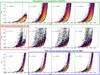 |
Fig. 22 Depth metrics for evaluating the performance of the ERO catalogues based on the photometric measurement error reported by SourceExtractor. The plot order from left to right is IE, YE, JE, and HE. Top row: field galaxies Kron photometry. SourceExtractor’s MAG_AUTO (Kron magnitude) provides the most accurate estimate of the total magnitude for galaxies in both VIS and NISP, using a conservative threshold of CLASS_STAR = 0.65 for star-galaxy separation (statistics from the ERO Abell 2390 field). Middle row: point sources PSF photometry for VIS. For stars, the VIS resolution facilitates effective separation of objects using SourceExtractor’s PSF-fitting photometry (MAG_PSF). However, this method is less effective with NISP, which tends to blend objects because of its coarser pixel scale, as evidenced by the scatter in comparison to VIS results; it also underestimates the photometric error on compact sources compared to aperture photometry (statistics from the ERO NGC 6397 field, also used on the bottom plot). Bottom row: point sources aperture photometry for NISP. A 1ʺ.2 diameter aperture is used for all objects in NISP (SourceExtractor’s MAG_APER), with the fitting tool selecting the deepest part of the distribution on the right, primarily composed of stars. An aperture correction is then applied to the numbers derived from such analyses, based on our analysis of enclosed energy (offsets: YE = –0.130, JE = –0.167, and HE = –0.249; refer to Table 1 for the aperture corrected values for NGC 6397 here). |
9.2 The observational Euclid extended PSF
9.2.1 Encompassed energy of the Euclid extended PSF
In analysing the extended PSF within the ERO data to estimate encircled energy up to a certain radius, we focused on the brightest star in the ERO fields, HD 1973 (V*BP Phoenicis, with AB magnitudes of 5.1 and 4.7 in the 2MASS J and H bands, see Fig. 23) near Abell 2764 (Atek et al. 2025). This star shows a prominent extended halo and distinct diffraction spikes that extend to large radii. Utilising AutoProf (Stone et al. 2021), a tool originally designed for galaxies, we conducted isopho- tal photometry on the PSF halo to obtain radial profiles in all four bands. By enforcing circular isophotes, we were able to extract a reliable signal up to 5ʹ.0 for VIS and 5ʹ.2 for NISP, ceasing at a surface brightness of 28.5 mag arcsec–2 for VIS and 30.0 mag arcsec–2 for NISP. Despite the star’s luminosity and the observation’s depth (three times the standard Euclid depth), we could not identify any signal beyond these extents and concluded we did reach the full extent of the extended PSF. HD 1973 approaches a magnitude close to Euclid’s threshold for avoiding such observations (4 AB mag in each band, see Euclid Collaboration: Scaramella et al. 2022), an indication that the telescope will have rare encounters with such stars in the EWS during its mission: the EWS is composed of 27571 pointings, with only 293 of them (1%) featuring a star IE < 5, and 1350 (5%) with a star HE < 5.
This star alone would be sufficient to characterise the extended PSF, except that the detector saturates in the brightest central regions of the stellar image (top left of the two profiles of Fig. 24). This information is needed to anchor the energy found in the extended halo to the energy found in the core of the PSF (Infante-Sainz et al. 2020; Liu et al. 2022). To extend the PSF brightness profile into the inner regions, as illustrated in Fig. 25, we extracted from single non-resampled frames a number of intermediate-brightness saturated stars, and some unsaturated stars, again using AutoProf to determine the profile of the PSF halo. For each profile (23 in total in each band) we manually determined the region in which the profile was robust by identifying clear features of saturation (a flattened profile in the inner regions) and the noise limit in the outskirts (that is high variance surface-brightness measurements).
For the key inner few pixels, we produced a pixel map with PSFex at 10× the native resolution, then converted to a radial profile using AutoProf. PSFex builds a complex polynomial model of the PSF through the analyses of thousands of bright unsaturated stars across a single non-resampled frame here, and captures key features of the Airy disc in all four bands in the ERO data.
With this strategy we average out second-order effects in the PSF – out to a radius of 10ʺ – caused by the different stellar spectral types in Euclid’s very broad photometric passbands. All of the profiles for the IE-band can be seen in the left panel of Fig. 25 where the stars have not yet been shifted from their original extraction. Using each profile only in the region where it was most robust, we performed an optimisation to rescale each profile until it aligned with the profile in star HD 1973. An example of this alignment for the IE-band can be seen in the middle panel of Fig. 25 where all the profiles are now aligned. We note that some profiles have no overlap with star HD 1973; however by simultaneously aligning all the profiles, we could bridge the gap from 300ʺ down to the sub-pixel level at the very core of the PSF. As a final step, we produced a collapsed profile which was the median of all profiles that contribute in a given region. This can be seen for the IE -band in the right panel of Fig. 25 which spans over four orders of magnitude in radius; the profile is normalised to μ0 = 0 by convention.
With this extended PSF available for all Euclid bands as shown in Fig. 26, we could then simply integrate the light to any radius and compare with the full integral. We find exceptional light enclosure for Euclid, with the values listed in Table 3 exceeding the original design specifications. VIS and NISP exhibit similar performance with about 90% of the encircled energy within a 1ʺ radius, 99% at 10ʺ, and 100% at 300ʺ. In Fig. 27 we compare our results with our simulations described in Appendix D, extending to the PSF core and verifying the accuracy of our data-based model. Given the basic assumptions of our theoretical PSF model, including ideal optics without phase variations or defects, this outcome underscores the effectiveness of Euclid’s optical design and fabrication quality.
In Fig. 26 simulations extending to larger radii are represented in blue. Across all four bands, there is a deviation from the extended wings of the Bessel-function characteristic of the Airy disc (r–3 slope) at large radius, with our simulation assuming an ideal circular pupil. Nevertheless, the slope measured from ERO data shows only a minor divergence from this ideal case of a pure diffraction halo and never reaches an r–2.5 slope. Such a slope would suggest a profile influenced by defects, dust, and various aberrations at the millimetre scale on the primary mirror, as discussed by Racine (1996). The observed dominance of optical diffraction over mirror surface roughness underscores the excellence of the manufacturing process and suggests that a negligible amount of particulates was deposited on the primary mirror during launch.
The extended PSF does not exhibit any obvious effects from the thin nanometre-scale layer of ice that accumulated on the optics near the VIS instrument after launch due to outgassing (Euclid Collaboration: Schirmer et al. 2023). Given that the VIS extended PSF contains less power in its halo compared to NISP, as shown in Fig. 26, we hypothesise that a portion of the PSF flux is uniformly extracted from the PSF and scattered isotropically, contributing to the overall background in the instrument’s cavity.
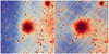 |
Fig. 23 VIS and NISP image of a very bright star. HD 1973, a fifth magnitude star in the HE-band (IE = 6.3, YE = 5.5, JE = 5.3, HE = 4.9), featured on a deep (3 ROS) ERO stack in the IE-band (left) and the HE- band (right) within a 23ʹ × 23ʹ field. The extended halo of VIS (left) concludes smoothly, exhibiting no detectable signal beyond a 5ʹ radius. Conversely, the NISP extended halo (right) terminates more abruptly – a characteristic of its refractive optics – yet also without a detectable signal past a 5ʹ radius. The diffraction spikes for VIS extend outward to approximately 12ʹ, whereas for NISP in HE-band they reach out to about 20ʹ. The very faint gradient observed in the background of the VIS image is attributed to stray light entering through the instrument platform rather than originating from the optical beam. |
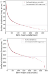 |
Fig. 24 Radial profile of HD 1973 on a deep (3 ROS) ERO stack in the IE -band (top) and the YE -band (bottom). These two profiles reveal distinct characteristics of the VIS and NISP instruments. For VIS, the extended halo concludes at a radius of 290ʺ, with AutoProf not detecting any signal beyond this point. In contrast, the NISP extended halo exhibits a notable excess of light at a radius of 260ʺ, indicative of its refractive optics (this feature is observable as a distinct arc in Fig. 23), and terminates shortly thereafter at a radius of 320ʺ. Cyan and red points refer to the colours of isophotes in an associated AutoProf visual, which help guide the eye when comparing plots. |
 |
Fig. 25 Left panel: analysed radial profiles of stars of varying brightness. We clipped the radius range to balance their contribution against the high-quality radial profile of HD 1973 (shown in green, upper right) and the high-S/N PSFex radial profile at the PSF core based on thousands of bright unsaturated stars (depicted in red, lower left). This approach ensured that the aggregate profile leverages both the detailed observation of a singularly bright star and the precision afforded by PSFex in the PSF’s core regions. Middle panel: optimisation step involved in aligning all profiles to achieve coherence across the data set. This optimisation process is critical for synthesising a unified radial profile from the disparate data points provided by stars of different magnitudes and the detailed profiles of HD 1973 and the PSF core. Right panel: final VIS extended PSF. The profile has been normalised to a base surface brightness of μ0 = 0 (corresponding in that case to a IE = 3.1 mag star). This standardised profile serves as a comprehensive model of the VIS PSF’s behaviour across a wide range of radii. |
9.2.2 Energy in the diffraction spikes
The PSF halo profiles, established through AutoProf employing median pixel values along the isophotes9, resulted in the initial analysis excluding the diffraction spike profiles from the PSF. However, these spikes represent a significant aspect of the PSF structure, and thus, the enclosed energy within the six spikes necessitates estimation in comparison to that derived from our ideal optical model. This step is crucial for a comprehensive understanding of the PSF’s energy distribution and for ensuring the accuracy of our extended-PSF model in reflecting the true performance of the optical system.
For our brightest star, HD 1973, we extracted all six spikes across each band, subsequently rotating and median-stacking them to produce a single, uncontaminated spike per band. This process ensured each spike was averaged across its entire width (3ʺ.6 for all bands), culminating in the profiles depicted in Fig. 28. The plot highlights the diffraction halo in lighter shades, clearly showing that the spike profiles exceed the halo’s brightness at large radii. Furthermore, it can be seen that the overall surface brightness escalates with increasing wavelength. The data align closely with our straightforward simulation (Appendix D), as illustrated in Fig. 28, particularly in terms of the relative brightness among the four bands, offering a vivid representation of the spike profiles’ luminance in comparison to the halo.
We assessed the total flux present in the diffraction spikes of HD 1973 relative to its overall brightness in the Euclid bands. This evaluation was facilitated by the extended PSF, which allows for accurate magnitude estimation of any saturated star by aligning its profile outside the saturated core. Our findings are in line with the initial simulation estimates: beyond a 10ʺ radius, the combined total-light fraction in both the spikes and the halo amounts to approximately 1.5% – averaging 1% for the halo and 0.5% for the spikes across all four bands. However, there is a notable distinction in their spatial distribution; the spikes are distinctly localised, whereas the halo extends azimuthally, covering a substantially larger area. In fact, at a 100" radius, the halo encompasses about two orders of magnitude more light than the spikes. Consequently, we opted not to incorporate the spike profiles into our extended PSF model, given our aim for percent-level accuracy in the results.
Encircled energy of the Euclid extended PSF.
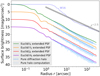 |
Fig. 26 Euclid’s extended PSF. The profiles across the four bands depicted with solid lines represent the stacked PSF, as detailed in Fig. 25, derived from ERO data. The IE-band is normalised to μ0 = 0, while the NISP YE, JE, and HE bands are visually separated by respective offsets of +5, +10, and +15 vertical units for clarity. The total magnitude of a star corresponding to each of the four profiles anchored at μ0 = 0 is IE = 3.1, YE = 1.6, JE = 1.5, and HE = 1.4 (it takes a brighter star in NISP to reach the same μ0 = 0 as VIS, which concentrates more energy in the core of the PSF, while the longer the wavelength, the poorer it becomes in the NIR). The simulation of the diffraction halo (Appendix D) is presented in pale blue, where the pale area represents the band-specific noisy computation profile and the dashed line indicates a second-order polynomial fit (an r–3 power law). This fit is aligned with the PSF at 2ʺ radius. The extended PSF concludes at 5ʹ radius, and its average slope shows only slight deviation from the theoretical model of a pure diffraction halo. This consistency underscores the exceptional quality of the optics, which appear to be free from particulate contamination. The three NIR extended PSFs are similar (constant offset between the purple, red, and orange profiles), but clearly contain more energy at large radii than the VIS extended PSF (the artificial 5 mag offset between the green and orange lines here quickly diminishes with radius). We represent in grey the median behaviour of all best wide-field LSB observatories reviewed by Liu et al. (2022) with an r–2.5 power law, shifted up to match our μ0 = 0, as originally done by Watkins et al. (2016). The specific extended V-band PSF of the Burrell Schmidt telescope is reproduced here (W16), as published in Watkins et al. (2016), limited to the range of this plot although it extends to a radius of 1°, ending at a surface brightness of 22.2 mag arcsec–2. This demonstrates that Euclid excels in minimising scattering of light, suppressing the extended wings better than the best ground-based optical telescopes by 8 magnitudes, and 6 magnitudes in the NIR, thereby opening a new observational window on the Universe. |
9.2.3 Consequence for the extended-emission science
Euclid boasts the most refined extended PSF ever achieved by a wide-field high-resolution imaging telescope. It sets a new benchmark far beyond past endeavours aimed at optimising telescopes for LSB science, a leap of 8 mag in minimising optical scattering of light in the optical while opening a whole new observational window in the NIR with a comparable leap of 6 mag in conjunction with the low background experienced at L2. See Figure 8 of Liu et al. (2022) review of the best optical LSB wide-field facilities around the world for an illustration, and our Fig. 26 for a comparison.
Characterised by an exceptionally high energy concentration in the PSF’s core, Euclid outperforms its predecessors and maintains this dominance within a nearly pure diffraction-halo regime extending up to a radius of 300ʺ, marking the boundary of the extended PSF’s influence. This unparalleled performance underscores Euclid’s revolutionary potential for astronomical observations in the realm of LSB science from the optical to the NIR.
Science focused on diffuse emission suffers through two main consequences of an extended PSF. First, bright stars in the FoV produce an accumulation of extended and overlapping halos that cause a modulation of the sky brightness, jeopardising the extraction of the LSB astronomical signal that gets lost in that non-flatness noise. Second, bright extended objects contaminate their own extended emission, for example a big elliptical galaxy biasing its radial profile by pushing light from its core into its stellar halo.
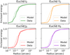 |
Fig. 27 Comparison of the encircled energy in the inner part (<10ʺ) of the extended PSF between measured data and a simulation of perfect optics for all four Euclid bands. The near match at the core, based on a PSFex profile from our sky data, indicates our extended PSF accurately reflects expected performance. The slight disagreement between the simple, aberration-free model and the data at a radius below 1ʺ (100) most likely stems from low-order aberrations introduced by optics. These aberrations tend to slightly broaden the core but have little to no effect on the extended PSF. The observation that the model-to- data discrepancy decreases with increasing wavelength tends to support this hypothesis, as optical aberrations are more pronounced at shorter wavelengths. It should be noted that the disagreement appears more pronounced due to the use of a log-log plot. |
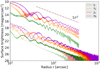 |
Fig. 28 Profiles of Euclid’s diffraction spikes. Diffraction spikes of the star HD 1973 analysed through photometric extraction profiles (at the bottom) juxtaposed with the star’s halo profile in a corresponding lighter shade (as illustrated in Fig. 26). This comparison highlights the pronounced dominance of spike brightness over the halo, becoming evident beyond a radius of a few arcseconds. Additionally, a simulation of the four spikes extending to a 400ʺ radius (with matching colours, and the HE-band arbitrarily set to μ0 = 10 for the purposes of this plot) corroborates the relative surface brightness of the spikes as observed across the four Euclid bands. Unlike the halo that adheres more closely to a 1/r3 function consistent with the Bessel envelope at high radius, the spike profiles, as anticipated, approximate a 1/r2 function. |
9.2.4 Contamination by overlapping stellar halos
The ERO field Abell 2764 – featuring the HE = 5 star HD 1973 – presents a scenario that Euclid will seldom face during its scientific mission. Despite its brightness, this star influences only about 0.022 deg2 (4%) of the 0.5 deg2 field through its extended diffusion halo. The predominant background component is the zodiacal light that averages around 22.2 mag arcsec–2, and the influence of the extended halo drops below 1% (equivalent to a 5 mag difference) at a radius of 200ʺ, as illustrated in Fig. 24.
To significantly affect the FoV at the 0.01% level at a radius of 200ʺ (which would be 1/100th of HD 1973’s impact, or 32 mag arcsec–2), one would need nearly 50 stars of magnitude 9 evenly scattered throughout the FoV. However, at worst across the entire EWS composed of 27 571 pointings, one pointing (0.004%) features at most 15 stars of this class (VIS or NISP), while on average across the EWS, the density of such stars amounts to just 2.8 per Euclid FoV.
Taking a more realistic perspective, considering the VIS saturation limit at magnitude 18.5 for long exposures and hypothesising the presence of one such star per square arcminute, the 1% level of zodiacal-light background (27.2 mag arcsec−2, a problematic level for LSB science) is attained within a radius of approximately 5ʺ, affecting merely 2% of a square arcminute. In even this pessimistic scenario, the overall impact on the detection of extended emission across scales of arcseconds and above, on average throughout the field, remains minimal. This analysis underscores Euclid’s robustness in handling the effects of bright stars on LSB science, facilitated by its advanced design.
Across the 17 ERO fields we encounter a range of stellar densities. Despite this variability, no field contains a sufficient number of stars to significantly impact the dominant zodiacal background. The noise in our images, across all scales, is primarily driven by photon statistics. Consequently, we deduce that our performance metric for assessing the LSB capabilities of our data set should concentrate exclusively on the zodiacal background’s brightness level. This approach remains applicable as long as the data processing is finely tuned for LSB science, as exemplified by the ERO pipeline. This optimisation ensures that the primary consideration in evaluating our LSB performance is the zodiacal light contribution, rather than the collective influence of stellar contributions and data processing signatures.
9.2.5 Self-contamination of a stellar halo
A potential issue in LSB science involves extended objects potentially contaminating their own signal (Slater et al. 2009; Karabal et al. 2017). This concern is particularly relevant when analysing large galaxies within the ERO science framework. However, due to Euclid’s exceptionally clean extended PSF, no correction for energy redistribution is necessary. For instance, the brightest surface-brightness levels (μ0) were measured for NGC 1549 and NGC 1553 in the ERO Dorado field, reaching approximately 14.3 mag arcsec–2 in the IE band. When incorporating the extended PSF (Fig. 26) at this brightness level, the self-contamination drops to around 30 mag arcsec–2 at a 10ʺ radius and to approximately 36 mag arcsec–2 at a 100ʺ radius. The minor energy redistribution caused by the extended PSF does not significantly impact ERO science. This is because most galaxies under study exceed in size the 99.7% encircled energy diameter of 2ʹ for both VIS and NISP, as detailed in Table 3. This is demonstrated in Fig. 29, where the impact of the convolution on two extended galaxies (one smaller and one larger than the extended PSF), leads to residuals at the sub-percent level. Consequently, the physical properties of these galaxies remain accurate, affirming that Euclid’s extended PSF allows for reliable LSB measurements without the need for adjustments for self-contamination.
9.2.6 Contamination by Galactic cirrus
A notable consideration in assessing Euclid’s LSB detection capabilities is that its actual limitation often stems from the interstellar medium foreground also known as Galactic cirrus (Sandage 1976). This phenomenon is detectable across all Galactic latitudes at present with optical wide-field cameras (Miville-Deschênes et al. 2016; Román et al. 2020; Lim et al. 2023), with brightness levels ranging between 26 and 28 mag arcsec–2. This factor is especially pertinent in the context of the ERO Perseus cluster of galaxies, where LSB performance is constrained by the non-uniformity of the background attributed to Galactic cirrus, as noted in studies such as Cuillandre et al. (2025); Kluge et al. (2025). The pronounced visibility of such cirrus, even in observations targeting HD 1973 (Fig. 23, left), underscores Euclid’s exceptional ability to discern extremely low-contrast LSB features, highlighting the challenge posed by the Galactic cirrus in accurately quantifying faint extragalactic astronomical signals. It is noteworthy that all 17 ERO fields showcased in Fig. B.1 easily reveal a faint background of Galactic cirrus in VIS even at high galactic latitudes.
9.3 LSB performance of the ERO data set
In Table B.2 we present the limiting surface brightness for each ERO field across the four Euclid bands, defining the anticipated depth for LSB science. This estimation is based on the assumption that the primary component of noise is pure photon statistics from the zodiacal light background, a justification rooted in the preceding discussions about the exceptional quality of the Euclid extended PSF. We determine the LSB depth metric following the methodology outlined in Euclid Collaboration: Scaramella et al. (2022), adapting the LSB asinh metric introduced by Mihos et al. (2013) deriving from the asinh metric for compact sources by Lupton et al. (1999), to more accurately mirror the real science capabilities in LSB-optimised images. This strategy aims to predict Euclid’s future performance in conducting LSB science with the understanding that the noise budget would primarily consist of photon-noise statistics from the zodiacal light. For a comprehensive explanation of this 1σ asinh AB magnitude metric applied at the 10ʺ × 10ʺ scale - used chiefly as a representative measure for various LSB scientific analyses – we refer to section 5.3 of Euclid Collaboration: Scaramella et al. (2022).
Adopting this metric, the ERO data set should theoretically achieve depths of IE = 29.9, YE = 28.2, JE = 28.4, and HE = 28.4 AB mag arcsec–2, averaged across the 17 fields, if aligning with predictions in Euclid Collaboration: Scaramella et al. (2022). These estimated depths (defined as limiting magnitudes in this paper) illustrate the capability to detect a 100 arcsec2 extended feature at the 1σ level based solely on photon statistics from the background, given the ultra-low impact of the extended PSF we have shown. However, direct measurements of physical features (such as stellar streams and cirrus) in the ERO images indicate that these limiting magnitudes appear to be optimistic by +0.4 mag (based on single ROS ERO observations), suggesting that the adoption of the asinh magnitude in Euclid Collaboration: Scaramella et al. (2022) was still not conservative enough and that unaccounted systematic errors, inherent to digital imaging and processing, are affecting the signal.
The consistency in depth across our collection is attributable to the ERO targets being located at ecliptic latitudes comparable to those surveyed by the EWS, as depicted in Fig. 1. The photometric catalogues from the first public release of the ERO data do not feature automated photometry for extended sources (scale above 10ʺ × 10ʺ). This functionality is slated for inclusion in the subsequent public data release, expanding the scope of scientific exploration enabled by Euclid.
As highlighted in the previous subsections, it is important to note that the LSB performance achieved for each individual ERO field is considerably influenced by the astronomical characteristics of the observed sky area, such as the presence of Galactic cirrus, stellar density, and – in certain instances – the density of large galaxies such as in the ERO Perseus field. These factors can substantially affect the ability to detect and analyse LSB features. The ERO Perseus cluster serves as a vivid illustration of how depth depends on the nature, scale, and analysis methods of specific astronomical entities: (i) the faintest dwarf galaxies in the new ERO Perseus cluster catalogue (Marleau et al. 2025) present a typical effective radius of 1ʺ and reach down to an average effective surface brightness of  mag arcsec–2, and a surface brightness at the effective radius of
  mag arcsec–2, at a total S/N within the effective radius high enough to enable derivation of physical parameters (S/N > 12, the performance being purely limited by background photon statistics at this scale); (ii) intracluster light reaches down to
  mag arcsec–2 at an S/N of 1 by integrating the signal over very large areas (Kluge et al. 2025); and (iii) radial profiles of galaxies go down to
  mag arcsec–2 (Cuillandre et al. 2025) when integrating light at increasing radii, by combining over 360 deg the signal of many 100 arcsec–2 areas, each at the S/N~2 level. The full suite of ERO papers related to LSB science provides a deeper understanding of the challenges and successes encountered in capturing and interpreting LSB phenomena within Euclid’s observations. For comprehensive insights into the actual scientific performance, we direct the reader to the first results of the ERO programme (Atek et al. 2025; Hunt et al. 2025; Martín et al. 2025; Massari et al. 2025; Saifollahi et al. 2025; Cuillandre et al. 2025; Kluge et al. 2025; Marleau et al. 2025). To encapsulate the main points of this section, Figs. 30 and 31 demonstrate Euclid’s unique capacity to detect and measure LSB features from the optical to the NIR.
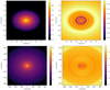 |
Fig. 29 Negligible impact of the extended PSF on physical parameters of very extended sources. Top-left panel: IE = 14 elliptical galaxy with a full extension less than that of the extended PSF (r = 300ʺ). Bottom-left panel: IE = 9 galaxy (NGC 1553) larger than the extended PSF. Right panels: relative variation of the flux redistribution after convolution with the extended PSF. The effect is at the sub-percent level and does not impact the derived physical properties such as their photometry or morphology. The colour intensity is in logarithmic scale in all four panels (-3.0 indicates a 10–3 ratio, or 0.1%). |
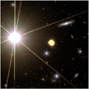 |
Fig. 30 Illustration of Euclid’s remarkable dynamic range, enabling LSB science. This paper quantifies Euclid’s capacity to measure faint extended emission in various ways. This capability is dramatically demonstrated through an extreme case where LSB features on the largest spiral galaxy in the top right corner are clearly visible, despite its proximity – just 2ʹ away - from HD 1973 (IE = 6.3, YE = 5.5, JE = 5.3, HE = 4.9). The field size is 3ʹ by 3ʹ. Faint galaxies are easily perceived within tens of arcseconds from this M3II star that is nearly visible to the naked eye: R=6.6 Vega magnitude, Pickles & Depagne (2010). This colour image was created by combining VIS and NISP data (without subtraction of the extended PSF model) using the IE-band for the blue, YE for the green, and HE for the red channel. The colour image at the NISP resolution is cast onto the VIS channel through a LAB (luminance + colours) combination to showcase the angular resolution and the sensitivity to LSB features. The oval structure at the centre is the result of a dichroic ghost in VIS caused by HD 1973 which appears yellow because the colour image is dominated at that distance from the star by the NISP extended PSF (green+red = yellow). |
10 Summary
We have described the ERO programme whose aim is to demonstrate Euclid’s capabilities before its primary mission. The programme focuses on 17 unique astronomical targets and employs a range of advanced technical methods to process the observations of these objects. The scientific results obtained for the individual targets are presented in a set of accompanying papers. Besides the overview of the ERO programme, the present paper has focused on the specific data processing that prepared the images for the individual ERO projects and an evaluation of Euclid’s unique LSB performance.
The ERO pipeline, which is crucial for creating data products for initial science studies, emphasises preserving data quality. The FWHM of the PSF in the advanced products (stacks) for the four Euclid channels shows a diffraction-limited telescope with 0ʺ.16 in the optical IE-band and 0ʺ.49 in the NIR bands YE, JE, and HE (Table 2). The point-source and extended-source detection limits with the Euclid survey nominal observing sequence match the pre-launch expectations of 25.3 and 23.2 AB mag with an S/N of ten for galaxies, and 27.1 and 24.5 AB mag at an S/N of five for point sources for VIS and NISP, respectively.
The pipeline’s main tasks involve removing instrumental signatures, calibrating astrometry and photometry, stacking images, and producing science-ready catalogues. Detrending involves several steps specific to each instrument to enhance image quality. For VIS, this includes using tools such as deepCR to remove CRs and maintain accurate astrometry. Similar steps are taken for NISP, including additional corrections of, for example, charge persistence and row-correlated noise. The zodiacal-light background is key for both instruments to be able to produce a flat-field that enables LSB science. Astrometric calibration starts by establishing an initial framework using Astrometry.net with Gaia-DR3 and is followed by refining global astrometry with SCAMP to address geometric distortions. Calibration accuracy is high, with VIS achieving a median internal precision of 6mas RMS, while NISP remains limited to 15 mas RMS due to its coarser sampling of the PSF.
External catalogues were used to refine the photometric zero points by making adjustments based on empirical data and synthetic photometry. The VIS calibration remains highly accurate, while NISP faces challenges due to model-dependent colour transformations. Detailed per-detector analysis in the VIS mosaic revealed statistically significant zero-point fluctuations, suggesting variability within and across detectors. The uncertainty of the VIS absolute flux calibration after tying it to Gaia averages better than 1%, with residual colour and brightness trends up to 10%. For NISP, calibration accuracy is capped at about 10% due to the model-dependent colour transformations and a limited early calibration data set.
The resampling and stacking process involved merging exposures using SWarp and produced two types of stacks: a background-removed stack for compact sources and a stack for studying extended emission. The choice of interpolating functions, such as the Lanczos3 kernel for VIS and bilinear interpolation for NISP, optimally preserves data quality. The PSF models were created using PSFex; however, the accuracy of these models is limited for NISP data by factors such as aliasing. The rich and detailed catalogues produced using SourceExtractor include extensive data from both VIS and NISP and are designed to support a broad range of scientific studies.
This ERO effort reveals that Euclid boasts the best extended PSF ever achieved by a wide-field high-resolution imaging telescope, setting a new benchmark that surpasses previous efforts to optimise telescopes for LSB science. It represents a leap of 8 magnitudes of surface brightness of the extended PSF halo in the optical range, and in particular, it opens a new observational window into the NIR LSB Universe, facilitated by the low background experienced at L2. The optical performance of Euclid indicates that the photometry of extended sources can be measured with high precision across the entire FoV without needing to deconvolve the image. In addition, the background of the Euclid images is dominated by photon noise across the entire image, confirming pre-launch expectations, and reaches a surface brightness for the nominal observing sequence of IE = 29.9, YE = 28.2, JE = 28.4, HE = 28.4 AB mag arcsec−2, which was achieved in the ERO data set for detecting a 100 arcsec2 extended feature at the 1 σ level (Table 2).
This first ERO data release includes science-ready source catalogues with a total of 11 million objects in the VIS and more than five million common detections in NISP across the 17 ERO fields. While this paper highlights this first release of the ERO data (stacks and catalogues) to the global scientific community, future ERO data releases will address existing challenges, such as photometry non-uniformity and improved stray light correction, and will introduce new features (e.g. automated LSB photometry) and possibly include a curated spectroscopy collection. This initial ERO release marks the beginning of a new era of scientific discoveries as Euclid embarks on its main mission.
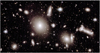 |
Fig. 31 Centre of the Abell 2764 cluster. Extended emission in the form of shells and stellar streams is traced in the NIR (colour image with IE-band in blue, YE in green, and HE in red) down to 27.0 mag arcsec−2 in the HE-band for a direct visual detection of physical features, such as a stellar stream, at 1 σ at the single square arcsecond scale. Structures within these faint features are well defined. The field size is 7ʹ by 3ʹ.5. |
Acknowledgements.
This work has made use of the Early Release Observations (ERO) data from the Euclid mission of the European Space Agency (ESA), 2024, https://doi.org/10.57780/esa-qmocze3. The Euclid Consortium acknowledges the European Space Agency and a number of agencies and institutes that have supported the development of Euclid, in particular the Agenzia Spaziale Italiana, the Austrian Forschungsförderungsgesellschaft funded through BMK, the Belgian Science Policy, the Canadian Euclid Consortium, the Deutsches Zentrum für Luft- und Raumfahrt, the DTU Space and the Niels Bohr Institute in Denmark, the French Centre National d’Etudes Spatiales, the Fundação para a Ciência e a Tecnologia, the Hungarian Academy of Sciences, the Ministerio de Ciencia, Innovación y Universidades, the National Aeronautics and Space Administration, the National Astronomical Observatory of Japan, the Netherlandse Onderzoekschool Voor Astronomie, the Norwegian Space Agency, the Research Council of Finland, the Romanian Space Agency, the State Secretariat for Education, Research, and Innovation (SERI) at the Swiss Space Office (SSO), and the United Kingdom Space Agency. A complete and detailed list is available on the Euclid web site (https://www.euclid-ec.org). This work presents results from the European Space Agency (ESA) space mission Gaia. Gaia data are being processed by the Gaia Data Processing and Analysis Consortium (DPAC). Funding for the DPAC is provided by national institutions, in particular the institutions participating in the Gaia MultiLateral Agreement (MLA). The Pan-STARRS1 Surveys (PS1) and the PS1 public science archive have been made possible through contributions by the Institute for Astronomy, the University of Hawaii, the Pan-STARRS Project Office, the Max-Planck Society and its participating institutes, the Max Planck Institute for Astronomy, Heidelberg and the Max Planck Institute for Extraterrestrial Physics, Garching, The Johns Hopkins University, Durham University, the University of Edinburgh, the Queen’s University Belfast, the Harvard-Smithsonian Center for Astrophysics, the Las Cumbres Observatory Global Telescope Network Incorporated, the National Central University of Taiwan, the Space Telescope Science Institute, the National Aeronautics and Space Administration under Grant No. NNX08AR22G issued through the Planetary Science Division of the NASA Science Mission Directorate, the National Science Foundation Grant No. AST–1238877, the University of Maryland, Eotvos Lorand University (ELTE), the Los Alamos National Laboratory, and the Gordon and Betty Moore Foundation. This project used public archival data from the Dark Energy Survey (DES). Funding for the DES Projects has been provided by the U.S. Department of Energy, the U.S. National Science Foundation, the Ministry of Science and Education of Spain, the Science and Technology Facilities Council of the United Kingdom, the Higher Education Funding Council for England, the National Center for Supercomputing Applications at the University of Illinois at Urbana- Champaign, the Kavli Institute of Cosmological Physics at the University of Chicago, the Center for Cosmology and Astro-Particle Physics at the Ohio State University, the Mitchell Institute for Fundamental Physics and Astronomy at Texas A&M University, Financiadora de Estudos e Projetos, Fundação Carlos Chagas Filho de Amparo à Pesquisa do Estado do Rio de Janeiro, Conselho Nacional de Desenvolvimento Científico e Tecnológico and the Ministério da Ciência, Tecnologia e Inovação, the Deutsche Forschungsgemeinschaft, and the Collaborating Institutions in the Dark Energy Survey. CS acknowledges the support of the Natural Sciences and Engineering Research Council of Canada (NSERC). Cette recherche a été financée par le Conseil de recherches en sciences naturelles et en génie du Canada (CRSNG). CS also acknowledges support from the Canadian Institute for Theoretical Astrophysics (CITA) National Fellowship program.
Appendix A Euclid ERO programme summary
Euclid ERO observations per proposal sorted by date.
Appendix B Euclid ERO data summary
Main characteristics and properties of the 17 ERO fields.
Sky coverage and depth properties for the 17 ERO fields.
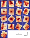 |
Fig. B.1 Seventeen ERO fields (approximately 0.6 deg2 each, IE preview). The blue frame encompasses the entirety of the FITS image for each science stack, guaranteeing that no quality Euclid data are omitted during projection into the equatorial coordinate system. Pixels identified as valid are those shared by both the VIS and NISP instruments. A dithering pattern impacted three fields – Taurus, NGC 6254, and IC 10 – resulting in incomplete sky coverage. The Fornax field is limited by having only two VIS exposures, leading to prominent gaps. Holmberg II, Fornax, and Dorado suffer from issues related to stray light, which will be addressed in the upcoming ERO data release. Any observed variations in the background of the remaining images stem from the LSB detection of Galactic nebulae (top row) or the presence of faint Galactic cirrus, illustrating the Euclid’s capability to easily capture these subtle astronomical features. |
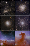 |
Fig. B.2 First set of five colour images released on 7 November 2023 that unveiled Euclid’s capabilities to the global community along with a cutout in the lower right (10ʹ × 10ʹ) that highlights the image resolution and depth achieved by Euclid. The images (cropped FoV= 0.5 deg2), starting from the top left, feature the Perseus cluster, IC 342, NGC 6822, NGC 6397, and the Horsehead Nebula. The pipeline detailed in this paper produced each of the three channels that contributed to the initial RGB images. These images were subsequently refined using external tools. The chosen colour palette assigns the IE, YE, and HE bands to the blue, green, and red channels respectively, displaying the full sensitivity range of the observatory and offering a new perspective on these astronomical subjects. Credit: ESA/Euclid/Euclid Consortium/NASA, image processing by J.-C. Cuillandre (CEA Paris-Saclay), G. Anselmi. |
Appendix C Selection of relevant stars along a given line of sight
Colour transformations for comparing Euclid photometry with existing literature are based on synthetic photometry of prevalent stars in the observation region, demonstrated through the Dorado and Perseus cases. Figure C.1 depicts outcomes from querying the Besançon model of the Galaxy (Robin et al. 2003; Czekaj 2012; Lagarde et al. 2021) for a 1 deg2 area towards NGC 1553, illustrating the process of deriving these transformations for accurate photometric comparisons. Both the Besançon model and the Planck 2013 dust map indicate an AV ≃ 0.04 in the direction of NGC 1553, suggesting that extinction effects are minimal and unlikely to be discernible in the figure. The right panels of the figure illustrate the models employed, with the SSED models represented by black open squares and the TSED models by black dots. It is important to note that [α/Fe] is explicitly considered only in the selection process for TSED models. Figure C.2 showcases the stellar populations expected along the line of sight towards Perseus, traversing extensive regio
 |
Fig. C.1 Relevant stars along the line of sight towards the Dorado field. This example showcases the selection process conducted prior to deriving colour transformations. The coloured dots depict the simulated stellar population along the line of sight, as provided by the Besançon model of the Galaxy. In the two left panels, the colour coding represents metallicity [M/H]. In the two right panels, the colour coding corresponds to [α/Fe], with black symbols marking the models available within the data-containing range of the simulation. Grey lines delineate the approximate boundaries we established for this selection process, ensuring that the subsequent colour transformations accurately reflect the characteristics of the stellar population along the observed line of sight. |
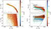 |
Fig. C.2 Relevant stars along the line of sight towards the Perseus field. The layout is as in Fig. C.1 |
Appendix D Optical model of the telescope
To accurately correlate the flux observed at large radii with the energy concentrated in the core of the PSF, a model of the Euclid PSF was developed. This modelling encompassed the broadband Euclid PSF across five distinct wavelengths, each representing the IE, YE, JE, and HE bands. The approach involved calculating the modulus squared of the Fourier transform of the pupil function, adhering to the Fraunhofer far-field diffraction approximation (Born & Wolf 1999). The pupil function represents the complex amplitude of light within the pupil, assuming ideal optical conditions without any phase term. Consequently, the pupil function equates to the real transmission of the pupil, designated as 1 inside the pupil’s boundary and 0 outside. The Euclid pupil was simulated on a substantial grid (16 384 × 16 384) using an outer diameter of 1.21 m for the primary mirror M1, a central obstruction of 0.395 m by the secondary mirror M2, and the width of 12mm for the three spider arms. The spiders are connected tangentially to the structure supporting M2 (see e.g. Racca et al. 2016).
D.1 Model of the encompassed energy of the Euclid PSF
To precisely determine the radial profile of the PSF by examining the cumulative flux fraction as a function of radius, we implemented a sampling strategy for our model PSF to achieve a resolution finer than 0ʺ.01. This necessitates oversampling by a factor of 5 relative to the Nyquist rate, resulting in a simulated field size of 2ʹ.5 × 2ʹ.5 on our 16384 × 16384 grid. Subsequently, we calculated the four Euclid broadband PSFs, adjusting the pupil sampling to ensure a consistent pixel scale across all wavelengths. This enabled us to calculate the proportion of total flux within a circular aperture of incrementally increasing radius, aligning these values with measurements extracted from the ERO data set.
For context, if we consider a perfect Airy disc for Euclid, the FWHM in radians is determined by the formula 1.025 × λ/D (M1), which yields the following FWHM values at the central wavelength for each of the four broadband filters: IE = 0ʺ.136, YE = 0ʺ.179, JE = 0ʺ.213, and HE = 0ʺ.298. This theoretical calculation aligns with the natural FWHM observed in VIS non-resampled data at the finer 0ʺ.1 pixel−1 sampling rate. However, the coarser 0ʺ.3 pixel−1 sampling rate of NISP degrades the observed FWHM, averaging approximately 0ʺ.41 across its three bands.
D.2 Energy in the diffraction spikes
Both VIS and NISP images display six pronounced diffraction spikes around bright stars, a result of the structure created by the three supporting spiders. In the case of a nearly 5th magnitude star, such as that seen in one of our ERO fields (Fig. 23), each spike stretches from 12ʹ in VIS to as much as 20ʹ in NISP for the HE-band. The extent of these spikes is influenced by the wavelength, with longer wavelengths exhibiting stronger effects and allowing for detection at greater distances. This phenomenon underscores two crucial points: first, the extended PSF is likely to have minimal power at large radii, evidenced by our ability to trace the spikes over substantial distances; second, there is a need to specifically model and measure the energy contained within the diffraction spikes for each Euclid band to affirm the methodology employed in determining the extended PSF.
A preliminary estimate of the total flux present in the diffraction pattern can be derived geometrically by calculating the area ratio of the spiders to the transmissive area, resulting in a value of 1.89%. However, due to the blinding effect of a 5th magnitude star on the ERO images, it is not feasible to directly measure this total quantity within a radius of 5ʺ from our images. Instead, the proportion of energy situated beyond a specific radius, which is quantifiable based on the ERO data, must initially be predicted through simulations. To simulate the fraction of flux from the central object located within the six diffraction spikes, we created the largest feasible field for our simulation grid, realised when the PSF is critically (Nyquist) sampled. In this scenario, the pupil diameter is halved in comparison to our grid size, rendering one pupil pixel equivalent to the diameter of M1 divided by our grid size: 148 microns on the primary mirror. This adjusted simulation extends to a radius of 7ʹ, with analyses of the ERO data suggesting that a significant portion of the energy within the spikes is contained within this radius. By creating identical pupil models both with and without the presence of spiders, we computed the corresponding PSFs, subtracted one from the other, and subsequently quantified the fraction of flux attributable to the spiders. In this way we ascertain the total fraction of flux from the central star located within all six diffraction spikes beyond a radius of 10ʺ, yielding the following percentages for each band: IE = 0.22%, YE = 0.41%, JE = 0.60%, and HE = 0.80%.
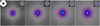 |
Fig. D.1 Main panels, from left to right: full 13ʹ × 13ʹ field simulated PSF in the IE, YE, JE, and HE bands in log scale; the core of the PSF in the inset (6ʺ ×6ʺ); and the pupil function in the top-left corner of the left panel. The pure diffraction halo grows larger towards the NIR. |
Appendix E ERO catalogue parameters by SourceExtractor
Input parameters for the SourceExtractor run producing the ERO science validation catalogues.
References
- Abbott, T. M. C., Adamów, M., Aguena, M., et al. 2021, ApJS, 255, 20 [NASA ADS] [CrossRef] [Google Scholar]
- Abraham, R. G., & van Dokkum, P. G. 2014, PASP, 126, 55 [Google Scholar]
- Antilogus, P., Astier, P., Doherty, P. E., Guyonnet, A., & Regnault, N. 2014, J. Instrum., 9, C03048 [Google Scholar]
- Atek, H., Gavazzi, R., Weaver, J. R., et al. 2025, A&A, 697, A15 (Euclid on Sky SI) [NASA ADS] [CrossRef] [EDP Sciences] [Google Scholar]
- Bertin, E. 2006, ASP Conf. Ser., 351, 112 [NASA ADS] [Google Scholar]
- Bertin, E. 2009, Mem. Soc. Astron. Italiana, 80, 422 [NASA ADS] [Google Scholar]
- Bertin, E. 2011, ASP Conf. Ser., 442, 435 [Google Scholar]
- Bertin, E., & Arnouts, S. 1996, A&AS, 117, 393 [NASA ADS] [CrossRef] [EDP Sciences] [Google Scholar]
- Bertin, E., Mellier, Y., Radovich, M., et al. 2002, ASP Conf. Ser., 281, 228 [Google Scholar]
- Bertin, E., Schefer, M., Apostolakos, N., et al. 2020, ASP Conf. Ser., 527, 461 [NASA ADS] [Google Scholar]
- Biesiadzinski, T., Lorenzon, W., Newman, R., et al. 2011, PASP, 123, 958 [Google Scholar]
- Boch, T., Pineau, F., & Derriere, S. 2012, ASP Conf. Ser., 461, 291 [NASA ADS] [Google Scholar]
- Born, M., & Wolf, E. 1999, Principles of optics: electromagnetic theory of propagation, interference and diffraction of light (Cambridge University Press) [CrossRef] [Google Scholar]
- Bougoin, M., Mallet, F., Lavenac, J., et al. 2018, SPIE Conf. Ser., 11180, 111801P-2 [Google Scholar]
- Bouy, H., Bertin, E., Moraux, E., et al. 2013, A&A, 554, A101 [NASA ADS] [CrossRef] [EDP Sciences] [Google Scholar]
- Carassou, S. 2017, PhD thesis, Université Pierre et Marie Curie – Paris VI, France [Google Scholar]
- Chambers, K. C., Magnier, E. A., Metcalfe, N., et al. 2016, arXiv e-prints [arXiv:1612.05560] [Google Scholar]
- Cuillandre, J.-C., Bolzonella, M., Boselli, A., et al. 2025, A&A, 697, A11 (Euclid on Sky SI) [Google Scholar]
- Cutri, R. M., Skrutskie, M. F., van Dyk, S., et al. 2003, VizieR Online Data Catalog: II/246 [Google Scholar]
- Czekaj, M. A. 2012, PhD thesis. University of Barcelona, Spain [Google Scholar]
- Dey, A., Schlegel, D. J., Lang, D., et al. 2019, AJ, 157, 168 [Google Scholar]
- Euclid Collaboration (Borlaff, A. S., et al.) 2022, A&A, 657, A92 [NASA ADS] [CrossRef] [EDP Sciences] [Google Scholar]
- Euclid Collaboration (Scaramella, R., et al.) 2022, A&A, 662, A112 [NASA ADS] [CrossRef] [EDP Sciences] [Google Scholar]
- Euclid Collaboration (Schirmer, M., et al.) 2022, A&A, 662, A92 [NASA ADS] [CrossRef] [EDP Sciences] [Google Scholar]
- Euclid Collaboration (Schirmer, M., et al.) 2023, A&A, 675, A142 [Google Scholar]
- Euclid Collaboration (Serrano, S., et al.) 2024, A&A, 690, A103 [NASA ADS] [CrossRef] [EDP Sciences] [Google Scholar]
- Euclid Collaboration (Cropper, M. S., et al.) 2025, A&A, 697, A2 (Euclid on Sky SI) [Google Scholar]
- Euclid Collaboration (Jahnke, K., et al.) 2025, A&A, 697, A3 (Euclid on Sky SI) [Google Scholar]
- Euclid Collaboration (Mellier, Y., et al.) 2025, A&A, 697, A1 (Euclid on Sky SI) [Google Scholar]
- Euclid Early Release Observations 2024, https://doi.org/10.57780/esa-qmocze3 [Google Scholar]
- Ferrarese, L., Côté, P., Cuillandre, J.-C., et al. 2012, ApJS, 200, 4 [Google Scholar]
- Fruchter, A. S., & Hook, R. N. 2002, PASP, 114, 144 [NASA ADS] [CrossRef] [Google Scholar]
- Gaia Collaboration (Prusti, T., et al.) 2016, A&A, 595, A1 [NASA ADS] [CrossRef] [EDP Sciences] [Google Scholar]
- Gaia Collaboration (Vallenari, A., et al.) 2023, A&A, 674, A1 [NASA ADS] [CrossRef] [EDP Sciences] [Google Scholar]
- Gaspar Venancio, L. M., Pachot, C., Carminati, L., et al. 2016, SPIE Conf. Ser., 9904, 99040P [Google Scholar]
- Gruen, D., Seitz, S., & Bernstein, G. M. 2014, PASP, 126, 158 [CrossRef] [Google Scholar]
- Hunt, L. K., Annibali, F., Cuillandre, J.-C., et al. 2025, A&A, 697, A9 (Euclid on Sky SI) [NASA ADS] [CrossRef] [EDP Sciences] [Google Scholar]
- Husser, T. O., Wende-von Berg, S., Dreizler, S., et al. 2013, A&A, 553, A6 [NASA ADS] [CrossRef] [EDP Sciences] [Google Scholar]
- Infante-Sainz, R., Trujillo, I., & Román, J. 2020, MNRAS, 491, 5317 [Google Scholar]
- Kalirai, J. S., Anderson, J., Richer, H. B., et al. 2007, ApJ, 657, L93 [Google Scholar]
- Karabal, E., Duc, P. A., Kuntschner, H., et al. 2017, A&A, 601, A86 [NASA ADS] [CrossRef] [EDP Sciences] [Google Scholar]
- Kluge, M. 2020, PhD thesis, Ludwig-Maximilians University of Munich, Germany [Google Scholar]
- Kluge, M., Hatch, N. A., Montes, M., et al. 2025, A&A, 697, A13 (Euclid on Sky SI) [NASA ADS] [CrossRef] [EDP Sciences] [Google Scholar]
- Korsch, D. 1977, Appl. Opt., 16, 2074 [NASA ADS] [CrossRef] [Google Scholar]
- Kubik, B., Barbier, R., Chabanat, E., et al. 2016, PASP, 128, 104504 [NASA ADS] [CrossRef] [Google Scholar]
- Kubik, B., Barbier, R., Smadja, G., et al. 2024, Proc. SPIE, 13103, 1310315 [Google Scholar]
- Lagarde, N., Reylé, C., Chiappini, C., et al. 2021, A&A, 654, A13 [NASA ADS] [CrossRef] [EDP Sciences] [Google Scholar]
- Lançon, A., Gonneau, A., Verro, K., et al. 2021, A&A, 649, A97 [NASA ADS] [CrossRef] [EDP Sciences] [Google Scholar]
- Lang, D., Hogg, D. W., Mierle, K., Blanton, M., & Roweis, S. 2010, AJ, 139, 1782 [Google Scholar]
- Lastennet, E., Lejeune, T., Oblak, E., Westera, P., & Buser, R. 2002, Ap&SS, 280, 83 [NASA ADS] [CrossRef] [Google Scholar]
- Laureijs, R., Amiaux, J., Arduini, S., et al. 2011, arXiv e-prints [arXiv:1110.3193] [Google Scholar]
- Le Graët, J., Secroun, A., Barbier, R., et al. 2022, SPIE Conf. Ser., 12191 [Google Scholar]
- Leinert, C., Bowyer, S., Haikala, L. K., et al. 1998, A&AS, 127, 1 [NASA ADS] [CrossRef] [EDP Sciences] [Google Scholar]
- Leisenring, J. M., Rieke, M., Misselt, K., & Robberto, M. 2016, Proc. SPIE, 9915, 99152N [Google Scholar]
- Lim, S., Hill, R., Scott, D., et al. 2023, MNRAS, 525, 1443 [Google Scholar]
- Liu, Q., Abraham, R., Gilhuly, C., et al. 2022, ApJ, 925, 219 [Google Scholar]
- Lupton, R. H., Gunn, J. E., & Szalay, A. S. 1999, AJ, 118, 1406 [Google Scholar]
- Magnier, E. A., & Cuillandre, J. C. 2004, PASP, 116, 449 [NASA ADS] [CrossRef] [Google Scholar]
- Marleau, F. R., Cuillandre, J.-C., Cantiello, M., et al. 2025, A&A, 697, A12 (Euclid on Sky SI) [NASA ADS] [CrossRef] [EDP Sciences] [Google Scholar]
- Marmo, C., & Bertin, E. 2008, ASP Conf. Ser., 394, 619 [Google Scholar]
- Martín, E. L., Žerjal, M., Bouy, H., et al. 2025, A&A, 697, A7 (Euclid on Sky SI) [NASA ADS] [CrossRef] [EDP Sciences] [Google Scholar]
- Massari, D., Dalessandro, E., Erkal, D., et al. 2025, A&A, 697, A8 (Euclid on Sky SI) [Google Scholar]
- McLeod, B. A., & Smith, R. 2016, SPIE Conf. Ser., 9915, 99150G [Google Scholar]
- Mihos, J. C., Harding, P., Feldmeier, J., & Morrison, H. 2005, ApJ, 631, L41 [Google Scholar]
- Mihos, J. C., Harding, P., Spengler, C. E., Rudick, C. S., & Feldmeier, J. J. 2013, ApJ, 762, 82 [NASA ADS] [CrossRef] [Google Scholar]
- Miville-Deschênes, M. A., Duc, P. A., Marleau, F., et al. 2016, A&A, 593, A4 [Google Scholar]
- Oke, J. B., & Gunn, J. E. 1983, ApJ, 266, 713 [NASA ADS] [CrossRef] [Google Scholar]
- Pickles, A. J. 1998, PASP, 110, 863 [NASA ADS] [CrossRef] [Google Scholar]
- Pickles, A., & Depagne, É. 2010, PASP, 122, 1437 [NASA ADS] [CrossRef] [Google Scholar]
- Pineau, F. X. 2020, ASP Conf. Ser., 527, 685 [Google Scholar]
- Pipien, S., Basa, S., Cuby, J. G., et al. 2018, A&A, 616, A55 [NASA ADS] [CrossRef] [EDP Sciences] [Google Scholar]
- Planck Collaboration XI. 2014, A&A, 571, A11 [NASA ADS] [CrossRef] [EDP Sciences] [Google Scholar]
- Powalka, M., Lançon, A., Puzia, T. H., et al. 2016, ApJS, 227, 12 [Google Scholar]
- Racca, G. D., Laureijs, R., Stagnaro, L., et al. 2016, SPIE Conf. Ser., 9904, 99040O [NASA ADS] [Google Scholar]
- Racine, R. 1996, PASP, 108, 699 [NASA ADS] [CrossRef] [Google Scholar]
- Regnault, N., Conley, A., Guy, J., et al. 2009, A&A, 506, 999 [NASA ADS] [CrossRef] [EDP Sciences] [Google Scholar]
- Robin, A. C., Reylé, C., Derrière, S., & Picaud, S. 2003, A&A, 409, 523 [NASA ADS] [CrossRef] [EDP Sciences] [Google Scholar]
- Rodrigo, C., & Solano, E. 2020, in XIV.0 Scientific Meeting (virtual) of the Spanish Astronomical Society, 182 [Google Scholar]
- Rodrigo, C., Solano, E., & Bayo, A. 2012, SVO Filter Profile Service Version 1.0, IVOA Working Draft 15 October 2012 [Google Scholar]
- Román, J., Trujillo, I., & Montes, M. 2020, A&A, 644, A42 [NASA ADS] [CrossRef] [EDP Sciences] [Google Scholar]
- Rothman, L., Gordon, I., Babikov, Y., et al. 2013, JQSRT, 130, 4 [NASA ADS] [CrossRef] [Google Scholar]
- Saifollahi, T., Voggel, K., Lançon, A., et al. 2025, A&A, 697, A10 (Euclid on Sky SI) [NASA ADS] [CrossRef] [EDP Sciences] [Google Scholar]
- Sandage, A. 1976, AJ, 81, 954 [Google Scholar]
- Sandin, C. 2014, A&A, 567, A97 [NASA ADS] [CrossRef] [EDP Sciences] [Google Scholar]
- Schlafly, E. F., Meisner, A. M., & Green, G. M. 2019, ApJS, 240, 30 [Google Scholar]
- Secroun, A., Barbier, R., Buton, C., et al. 2018, SPIE Conf. Ser., 10709, 1070921 [Google Scholar]
- Serra, B., Secroun, A., Clémens, J. C., et al. 2015, SPIE Conf. Ser., 9602, 96020G [Google Scholar]
- Slater, C. T., Harding, P., & Mihos, J. C. 2009, PASP, 121, 1267 [Google Scholar]
- Smith, R. M., Zavodny, M., Rahmer, G., & Bonati, M. 2008, SPIE Conf. Ser., 7021, 70210J [NASA ADS] [Google Scholar]
- Stone, C. J., Arora, N., Courteau, S., & Cuillandre, J.-C. 2021, MNRAS, 508, 1870 [NASA ADS] [CrossRef] [Google Scholar]
- Szalay, A. S., Connolly, A. J., & Szokoly, G. P. 1999, AJ, 117, 68 [Google Scholar]
- Taylor, M. B. 2005, ASP Conf. Ser., 347, 29 [Google Scholar]
- Tulloch, S. 2018, arXiv e-prints [arXiv:1807.05217] [Google Scholar]
- van Dokkum, P. G. 2001, PASP, 113, 1420 [Google Scholar]
- Waczynski, A., Barbier, R., Cagiano, S., et al. 2016, SPIE Conf. Ser., 9915, 991511 [NASA ADS] [Google Scholar]
- Watkins, A. E., Mihos, J. C., & Harding, P. 2016, ApJ, 826, 59 [Google Scholar]
- Zhang, K., & Bloom, J. S. 2020, ApJ, 889, 24 [NASA ADS] [CrossRef] [Google Scholar]
The colours of the models of Pickles (1998) also align with those shown in Fig. 19.
Gaia transmission curves were obtained via the SVO service (see note 6) in September 2023 and verified to match those described at https://www.cosmos.esa.int/web/gaia/dr3-passbands
The SVO Vega spectrum was compared to various Vega model versions available at the Space Telescope Science Institute (https://ssb.stsci.edu/cdbs/calspec/), and was found to be identical to alpha_lyr_stis_010 at wavelengths below 1 μm and within a few mmag of alpha_lyr_stis_011 at longer wavelengths.
All Tables
General median properties of the 17 Euclid ERO fields with a 0.60 deg2 sky coverage for single ROS observations.
Input parameters for the SourceExtractor run producing the ERO science validation catalogues.
All Figures
|
Fig. 1 Location, name, and nature of the 17 ERO fields on an all-sky map. The general RoI of the EWS is highlighted by the four blue contours. These outlines signify that some of the ERO targets will be revisited in the coming years. The distinctive nature of the ERO programme facilitated explorations spanning from the Galactic plane to the southern Galactic cap, areas that were accessible during the observation period. This range of coverage showcases the ERO programme’s goal to venture across a wide variety of astronomical phenomena and regions. The blue background depicts the stellar density across the sky. |
| In the text | |
|
Fig. 2 Left: single raw VIS bias frame captured at L2. The image exhibits numerous CRs, and has been corrected with a fixed pedestal level per quadrant based on the median value in the overscan area. Right: correction using a smoothed vertical vector of the overscan area. The contrast here is maximised to highlight effects at the sub-ADU level. The solution adopted on the right still exhibits an instrumental signature (some quadrants, or entire detectors, have a non-zero signal), necessitating an additional two-dimensional bias correction. |
| In the text | |
|
Fig. 3 Left: features of a CCD quadrant. This quadrant from a raw bias image shows (i) a noticeable jump in the readout pedestal during readout (with more subtle variations observable throughout the readout), (ii) a top-down intensity gradient indicative of light injection during readout, and (iii) an electronic ringing effect on the left at the start of each line readout. Right: high-S/N master bias frame (median of tens of raw images) used to process all ERO data. The brightness variation here does not exceed 0.6 ADU, while the typical raw ERO signal – zodiacal light background – is around 40 ADUs, necessitating this correction. |
| In the text | |
|
Fig. 4 ERO zodiacal light flat-field. This is a combination of large scales (>10ʺ) derived solely from the zodiacal light observed in any long VIS exposures and small scales (<10ʺ) coming from a weighted average of five high-S/N LED internal calibration images. These have wavelengths of 573 nm, 610 nm, 660 nm, 720 nm, and 890 nm, matching spectral coverage of VIS. The colour scale is arbitrary, set to explore the full range of intensity within each image. The top five images show the wavelength-dependent evolution of {gain × quantum efficiency}. This large-scale pattern is removed in the flat-field, replaced by the one from the pure zodiacal light image (bottom left). The overall left-to-right gradient is caused by the telescopic off-axis illumination and the VIS shutter effect (see also Euclid Collaboration: Cropper et al. 2025). The final ERO VIS zodiacal flat-field (bottom centre) incorporates all scales present in the Euclid signal, from pixel-to-pixel sensitivity variations (bottom right, highlighting a quadrant covering 205ʺ × 206ʺ, with a zoom on a 30 by 30 pixels area showing the pixel-to-pixel sensitivity differences) to the scale of the FoV. |
| In the text | |
|
Fig. 5 Left: detrended VIS image of the Perseus cluster. This image follows the ERO mask, overscan, bias, flat-field, and deepCR corrections revealing a checkerboard pattern in a small number of quadrants, which is noticeable through the subtle relative jumps of the background level between adjacent quadrants. The effect is 2% of the background for the two most affected quadrants (if left uncorrected this would leave residuals at the 27 to 28th mag arcsec−2 level). Right: final image after applying a low-flux nonlinearity correction to approximately 30 quadrants. The image now displays uniform flatness of the background across all borders – both between detectors and within quadrants – indicating reliable photometry for extended emission such as galaxy stellar halos, intra-cluster light, and Galactic cirrus, as showcased here. The limiting surface brightness of these single frames exceeds 29 mag arcsec−2 throughout the entire FoV (direct detection of faint contrasts at the 10ʺ scale). |
| In the text | |
|
Fig. 6 Top panel: histogram of all pixels across a 200 arcsec2 region from a VIS detrended image. The histogram shows regular spikes at the 1 ADU frequency, indicative of quantisation noise (this effect is also observed in the raw data). Bottom panel: same region after resampling the detrended image with SWarp using a Lanczos3 function. The histogram shows that the pixels have been correlated and the quantisation error has been smoothed out. |
| In the text | |
|
Fig. 7 Identification and removal procedure of the CR contamination. Images showing that the Python-based machine learning-driven tool deepCR effectively identifies (centre) and repairs (bottom) pixels affected by CRs (top). Each image segment (single rectangle) measures 2ʹ × 1ʹ, demonstrating deepCR’s effectiveness in enhancing image quality. |
| In the text | |
|
Fig. 8 Impact of deepCR corrections on photometric accuracy. Magnitude difference between the input synthetic stars and their measured photometry after applying deepCR masking and in-painting plotted against the input magnitude (using an arbitrary zero point). The colour scale on the graph represents the number of pixels within a 25-pixel aperture diameter that were affected by CRs. On the right side of the graph, a histogram displays the distribution of the magnitude differences, providing a visual representation of the photometric accuracy and the impact of CR corrections across various levels of CR contamination. |
| In the text | |
|
Fig. 9 Release rate Ṙ for an example pixel derived from an LED flat with a subsequent series of dark exposures. The data points show the persistence signal P in the dark images with the bias pedestal (1024 ADU) subtracted and normalised by the exposure time and initial signal S . The horizontal error bars mark the beginning and end of each dark exposure. The best-fit power law (A = −1.215, B = −1.829) is shown in blue. |
| In the text | |
|
Fig. 10 Persistence model parameters for NISP detector 1. The parameters A and B are defined in Eq. (1). The correction factor K is shown for the date 2023-09-16. It is defined in Eq. (3). |
| In the text | |
|
Fig. 11 Example region in the Perseus ERO JE-band stack before (left) and after (right) subtracting the predicted persistence from the single exposures. White corresponds to a surface brightness of approximately 25 mag arcsec−2. |
| In the text | |
|
Fig. 12 Dark current map for the 16 NISP detectors. The final map is derived from a stack of 110-s integration dark frames that match the duration of the science exposures. The amplitude of the dark current varies, reaching up to 1.6 ADU at most across a single detector and with an average value of 0.8 ADU across the entire mosaic. The minimum in dark blue is 0.0 ADU; the maximum in deep red is 2.6 ADU. |
| In the text | |
|
Fig. 13 ERO NISP zodiacal light flat-field. This combines the large scales (>80ʺ) derived solely from zodiacal light observed in any NISP exposures with the small and medium scales (<80ʺ) coming from specific LED internal calibration images tailored to each NISP band (only three LEDs were relevant for this purpose: 1160 nm, 1470 nm, and 1720 nm for YE, JE, HE, respectively). The arbitrary colour scale is used to fully explore the intensity range within each image. The top row displays the evolution of {gain × quantum efficiency} across all 16 NISP detectors at specific wavelengths, highlighting a large-scale pattern that is, however, omitted in the final flat-field in preference to the pattern emanating from the zodiacal light image (bottom left). The completed ERO NISP zodiacal flat-field (bottom centre, for HE) encapsulates all scales present in the Euclid signal, ranging from pixel-to-pixel sensitivity variations and low-to-medium-sized features (bottom right, showing a detector of 612ʺ × 612ʺ, with a zoom on a 30 by 30 pixels area showing the pixel-to-pixel sensitivity differences), extending to the entire FoV scale. The relative colour range from dark blue to deep red is an intensity ratio of 12% on average across the full mosaic panels and 5% for the variations across the single detector on the lower right. |
| In the text | |
|
Fig. 14 Left: original image (900 px× 1200 px area of a single NISP detector). Horizontal striping indicative of row-correlated noise is easily noticeable. Middle: noise model constructed spanning the image’s width to specifically target and quantify the noise pattern. Right: corrected frame where the row-correlated noise has been mitigated. This image demonstrates that the procedure effectively addresses the noise issue without substantially impacting the extended emission in the image. The residual image persistence caused by the NISP spectra generates an apparent column-correlated noise. |
| In the text | |
|
Fig. 15 Post-calibration astrometric residuals along the RA and Dec axes for unsaturated Gaia-DR3 stars in the NGC 6397 field (Massari et al. 2025). Residuals were computed for each star as the difference between the calibrated coordinates on the individual VIS exposures and the corrected Gaia-DR3 coordinates (see text). Grey points represent a subsample of detections with a S/N > 100 on ERO exposures. The plot reveals two distinct groups of stars, represented as a large cloud slightly offset from the centre and a small compact cloud clearly separated from the centre, both consisting of stars lacking proper motion data in the DR3 catalogue. The position offset of the smaller ‘cloud’, located in the lower left, aligns well with previous estimates of the NGC 6397 absolute proper motion (μ* = (3.6,−17.3) mas yr−1, Kalirai et al. 2007), over a period of 7.7 years. A dashed square at the centre of the plot illustrates the size of the VIS pixel footprint for comparison. On this specific ERO field the internal astrometric precision is 2.7 mas RMS. |
| In the text | |
|
Fig. 16 Top: (left to right) ERO Perseus cluster in the HE-band (full FoV of 0.70 deg2) showing the extended emission stack, compact-sources stack, and weight map (all in inverted scale). Bottom (left to right): ERO Horsehead Nebula in the IE-band (full FoV of 0.59 deg2) showing the extended emission stack, compact-sources stack, and weight map (all in inverted scale). All ERO fields are rotated to deliver a standard equatorial projection where north is up and east is to the left. The main difference between the two types of stacks (center versus left) is the suppression of extended emission in the compact-sources stack to optimise compact source photometry. The two flavours of stacking are motivated by the need to optimise the photometry for each class of objects (it is not recommended to use the extended-emission stacks for compact-source science). The weight maps echo the observing strategy, with a S/N that can vary greatly across the image. This is particularly striking on the bottom right, based on a standard Euclid observing sequence. |
| In the text | |
|
Fig. 17 Common FoV of VIS and NISP. This image was generated from two VIS and NISP images taken simultaneously with common astrometry applied. The small blue numbers refer to VIS, and the large red numbers refer to NISP detector IDs. The interchip gaps of each mosaic is evident. The VIS detectors show an additional thin horizontal gap from the charge-injection lines. The respective spatial and angular offsets between both instruments are 52ʺ.5 and 0°.078. Figure from Euclid Collaboration: Mellier et al. (2025). |
| In the text | |
|
Fig. 18 Spectral response of Euclid’s wide imaging bands. For comparison we show the Gaia bands that we used – among others – for photometric calibration of the VIS IE-band, and the atmospheric transmission that limits the ground-based Y, J, H, and Ks bands, for a precipitable water vapour level of 1.0 mm from Rothman et al. (2013). Considerable colour terms may arise for individual sources when transforming fluxes in the wide Euclid bands to fluxes in other photometric systems. |
| In the text | |
|
Fig. 19 Calibration of IE against Gaia. The upper panels display the colour transformation between Gaia-DR3 photometry (converted to the AB magnitude system) and IE for Milky-Way stars in the ERO fields towards Dorado (left panel), Perseus (middle), and NGC 2403 (right). In the lower sub-panels, the residual difference between the predicted and observed IE photometry is plotted. The coloured symbols represent observations, as determined from stacked images using photometry in a large aperture and the pre-launch ZP, that is a stack ZP of 30 as described in Sect. 7. An average foreground extinction is applied to the synthetic photometry, as adequate for each line of sight; the empirical data have not been dereddened. Two extinction vectors are shown in each figure, both for AV = 0.5, with one appropriate for the bluest stars and one for the reddest ones. Coincidentally the extinction vector is almost aligned with the colour-transformation curve at all colours; as a result extinction corrections of up to AV = 1 change IE,obs − IE,pred by less than 0.01 magnitude. |
| In the text | |
|
Fig. 20 Illustration of the IE magnitude offset with respect to pre-launch estimates of the ZP, per detector, using one exposure on the Perseus galaxy cluster. The horizontal line indicates the average offset, while the green symbols represent stars with a Gaia colour of (GBP – GRP) < 1.8. These stars were specifically used to calculate the average offset, highlighting the variations across different detectors and emphasising the impact of stellar colours on the observed magnitudes. |
| In the text | |
|
Fig. 21 Colour transformation between DES and Euclid NISP photometry for Dorado (top) and between PS1 and Euclid NISP photometry for Perseus (bottom). The figure setup is as in Fig. 19. Extinction is applied to the synthetic magnitudes (AV = 0.05 mag in the case of Dorado, AV = 0.45 mag in the case of Perseus), and a typical extinction vector for AV = 0.5 mag is also shown. |
| In the text | |
|
Fig. 22 Depth metrics for evaluating the performance of the ERO catalogues based on the photometric measurement error reported by SourceExtractor. The plot order from left to right is IE, YE, JE, and HE. Top row: field galaxies Kron photometry. SourceExtractor’s MAG_AUTO (Kron magnitude) provides the most accurate estimate of the total magnitude for galaxies in both VIS and NISP, using a conservative threshold of CLASS_STAR = 0.65 for star-galaxy separation (statistics from the ERO Abell 2390 field). Middle row: point sources PSF photometry for VIS. For stars, the VIS resolution facilitates effective separation of objects using SourceExtractor’s PSF-fitting photometry (MAG_PSF). However, this method is less effective with NISP, which tends to blend objects because of its coarser pixel scale, as evidenced by the scatter in comparison to VIS results; it also underestimates the photometric error on compact sources compared to aperture photometry (statistics from the ERO NGC 6397 field, also used on the bottom plot). Bottom row: point sources aperture photometry for NISP. A 1ʺ.2 diameter aperture is used for all objects in NISP (SourceExtractor’s MAG_APER), with the fitting tool selecting the deepest part of the distribution on the right, primarily composed of stars. An aperture correction is then applied to the numbers derived from such analyses, based on our analysis of enclosed energy (offsets: YE = –0.130, JE = –0.167, and HE = –0.249; refer to Table 1 for the aperture corrected values for NGC 6397 here). |
| In the text | |
|
Fig. 23 VIS and NISP image of a very bright star. HD 1973, a fifth magnitude star in the HE-band (IE = 6.3, YE = 5.5, JE = 5.3, HE = 4.9), featured on a deep (3 ROS) ERO stack in the IE-band (left) and the HE- band (right) within a 23ʹ × 23ʹ field. The extended halo of VIS (left) concludes smoothly, exhibiting no detectable signal beyond a 5ʹ radius. Conversely, the NISP extended halo (right) terminates more abruptly – a characteristic of its refractive optics – yet also without a detectable signal past a 5ʹ radius. The diffraction spikes for VIS extend outward to approximately 12ʹ, whereas for NISP in HE-band they reach out to about 20ʹ. The very faint gradient observed in the background of the VIS image is attributed to stray light entering through the instrument platform rather than originating from the optical beam. |
| In the text | |
|
Fig. 24 Radial profile of HD 1973 on a deep (3 ROS) ERO stack in the IE -band (top) and the YE -band (bottom). These two profiles reveal distinct characteristics of the VIS and NISP instruments. For VIS, the extended halo concludes at a radius of 290ʺ, with AutoProf not detecting any signal beyond this point. In contrast, the NISP extended halo exhibits a notable excess of light at a radius of 260ʺ, indicative of its refractive optics (this feature is observable as a distinct arc in Fig. 23), and terminates shortly thereafter at a radius of 320ʺ. Cyan and red points refer to the colours of isophotes in an associated AutoProf visual, which help guide the eye when comparing plots. |
| In the text | |
|
Fig. 25 Left panel: analysed radial profiles of stars of varying brightness. We clipped the radius range to balance their contribution against the high-quality radial profile of HD 1973 (shown in green, upper right) and the high-S/N PSFex radial profile at the PSF core based on thousands of bright unsaturated stars (depicted in red, lower left). This approach ensured that the aggregate profile leverages both the detailed observation of a singularly bright star and the precision afforded by PSFex in the PSF’s core regions. Middle panel: optimisation step involved in aligning all profiles to achieve coherence across the data set. This optimisation process is critical for synthesising a unified radial profile from the disparate data points provided by stars of different magnitudes and the detailed profiles of HD 1973 and the PSF core. Right panel: final VIS extended PSF. The profile has been normalised to a base surface brightness of μ0 = 0 (corresponding in that case to a IE = 3.1 mag star). This standardised profile serves as a comprehensive model of the VIS PSF’s behaviour across a wide range of radii. |
| In the text | |
|
Fig. 26 Euclid’s extended PSF. The profiles across the four bands depicted with solid lines represent the stacked PSF, as detailed in Fig. 25, derived from ERO data. The IE-band is normalised to μ0 = 0, while the NISP YE, JE, and HE bands are visually separated by respective offsets of +5, +10, and +15 vertical units for clarity. The total magnitude of a star corresponding to each of the four profiles anchored at μ0 = 0 is IE = 3.1, YE = 1.6, JE = 1.5, and HE = 1.4 (it takes a brighter star in NISP to reach the same μ0 = 0 as VIS, which concentrates more energy in the core of the PSF, while the longer the wavelength, the poorer it becomes in the NIR). The simulation of the diffraction halo (Appendix D) is presented in pale blue, where the pale area represents the band-specific noisy computation profile and the dashed line indicates a second-order polynomial fit (an r–3 power law). This fit is aligned with the PSF at 2ʺ radius. The extended PSF concludes at 5ʹ radius, and its average slope shows only slight deviation from the theoretical model of a pure diffraction halo. This consistency underscores the exceptional quality of the optics, which appear to be free from particulate contamination. The three NIR extended PSFs are similar (constant offset between the purple, red, and orange profiles), but clearly contain more energy at large radii than the VIS extended PSF (the artificial 5 mag offset between the green and orange lines here quickly diminishes with radius). We represent in grey the median behaviour of all best wide-field LSB observatories reviewed by Liu et al. (2022) with an r–2.5 power law, shifted up to match our μ0 = 0, as originally done by Watkins et al. (2016). The specific extended V-band PSF of the Burrell Schmidt telescope is reproduced here (W16), as published in Watkins et al. (2016), limited to the range of this plot although it extends to a radius of 1°, ending at a surface brightness of 22.2 mag arcsec–2. This demonstrates that Euclid excels in minimising scattering of light, suppressing the extended wings better than the best ground-based optical telescopes by 8 magnitudes, and 6 magnitudes in the NIR, thereby opening a new observational window on the Universe. |
| In the text | |
|
Fig. 27 Comparison of the encircled energy in the inner part (<10ʺ) of the extended PSF between measured data and a simulation of perfect optics for all four Euclid bands. The near match at the core, based on a PSFex profile from our sky data, indicates our extended PSF accurately reflects expected performance. The slight disagreement between the simple, aberration-free model and the data at a radius below 1ʺ (100) most likely stems from low-order aberrations introduced by optics. These aberrations tend to slightly broaden the core but have little to no effect on the extended PSF. The observation that the model-to- data discrepancy decreases with increasing wavelength tends to support this hypothesis, as optical aberrations are more pronounced at shorter wavelengths. It should be noted that the disagreement appears more pronounced due to the use of a log-log plot. |
| In the text | |
|
Fig. 28 Profiles of Euclid’s diffraction spikes. Diffraction spikes of the star HD 1973 analysed through photometric extraction profiles (at the bottom) juxtaposed with the star’s halo profile in a corresponding lighter shade (as illustrated in Fig. 26). This comparison highlights the pronounced dominance of spike brightness over the halo, becoming evident beyond a radius of a few arcseconds. Additionally, a simulation of the four spikes extending to a 400ʺ radius (with matching colours, and the HE-band arbitrarily set to μ0 = 10 for the purposes of this plot) corroborates the relative surface brightness of the spikes as observed across the four Euclid bands. Unlike the halo that adheres more closely to a 1/r3 function consistent with the Bessel envelope at high radius, the spike profiles, as anticipated, approximate a 1/r2 function. |
| In the text | |
|
Fig. 29 Negligible impact of the extended PSF on physical parameters of very extended sources. Top-left panel: IE = 14 elliptical galaxy with a full extension less than that of the extended PSF (r = 300ʺ). Bottom-left panel: IE = 9 galaxy (NGC 1553) larger than the extended PSF. Right panels: relative variation of the flux redistribution after convolution with the extended PSF. The effect is at the sub-percent level and does not impact the derived physical properties such as their photometry or morphology. The colour intensity is in logarithmic scale in all four panels (-3.0 indicates a 10–3 ratio, or 0.1%). |
| In the text | |
|
Fig. 30 Illustration of Euclid’s remarkable dynamic range, enabling LSB science. This paper quantifies Euclid’s capacity to measure faint extended emission in various ways. This capability is dramatically demonstrated through an extreme case where LSB features on the largest spiral galaxy in the top right corner are clearly visible, despite its proximity – just 2ʹ away - from HD 1973 (IE = 6.3, YE = 5.5, JE = 5.3, HE = 4.9). The field size is 3ʹ by 3ʹ. Faint galaxies are easily perceived within tens of arcseconds from this M3II star that is nearly visible to the naked eye: R=6.6 Vega magnitude, Pickles & Depagne (2010). This colour image was created by combining VIS and NISP data (without subtraction of the extended PSF model) using the IE-band for the blue, YE for the green, and HE for the red channel. The colour image at the NISP resolution is cast onto the VIS channel through a LAB (luminance + colours) combination to showcase the angular resolution and the sensitivity to LSB features. The oval structure at the centre is the result of a dichroic ghost in VIS caused by HD 1973 which appears yellow because the colour image is dominated at that distance from the star by the NISP extended PSF (green+red = yellow). |
| In the text | |
|
Fig. 31 Centre of the Abell 2764 cluster. Extended emission in the form of shells and stellar streams is traced in the NIR (colour image with IE-band in blue, YE in green, and HE in red) down to 27.0 mag arcsec−2 in the HE-band for a direct visual detection of physical features, such as a stellar stream, at 1 σ at the single square arcsecond scale. Structures within these faint features are well defined. The field size is 7ʹ by 3ʹ.5. |
| In the text | |
|
Fig. B.1 Seventeen ERO fields (approximately 0.6 deg2 each, IE preview). The blue frame encompasses the entirety of the FITS image for each science stack, guaranteeing that no quality Euclid data are omitted during projection into the equatorial coordinate system. Pixels identified as valid are those shared by both the VIS and NISP instruments. A dithering pattern impacted three fields – Taurus, NGC 6254, and IC 10 – resulting in incomplete sky coverage. The Fornax field is limited by having only two VIS exposures, leading to prominent gaps. Holmberg II, Fornax, and Dorado suffer from issues related to stray light, which will be addressed in the upcoming ERO data release. Any observed variations in the background of the remaining images stem from the LSB detection of Galactic nebulae (top row) or the presence of faint Galactic cirrus, illustrating the Euclid’s capability to easily capture these subtle astronomical features. |
| In the text | |
|
Fig. B.2 First set of five colour images released on 7 November 2023 that unveiled Euclid’s capabilities to the global community along with a cutout in the lower right (10ʹ × 10ʹ) that highlights the image resolution and depth achieved by Euclid. The images (cropped FoV= 0.5 deg2), starting from the top left, feature the Perseus cluster, IC 342, NGC 6822, NGC 6397, and the Horsehead Nebula. The pipeline detailed in this paper produced each of the three channels that contributed to the initial RGB images. These images were subsequently refined using external tools. The chosen colour palette assigns the IE, YE, and HE bands to the blue, green, and red channels respectively, displaying the full sensitivity range of the observatory and offering a new perspective on these astronomical subjects. Credit: ESA/Euclid/Euclid Consortium/NASA, image processing by J.-C. Cuillandre (CEA Paris-Saclay), G. Anselmi. |
| In the text | |
|
Fig. C.1 Relevant stars along the line of sight towards the Dorado field. This example showcases the selection process conducted prior to deriving colour transformations. The coloured dots depict the simulated stellar population along the line of sight, as provided by the Besançon model of the Galaxy. In the two left panels, the colour coding represents metallicity [M/H]. In the two right panels, the colour coding corresponds to [α/Fe], with black symbols marking the models available within the data-containing range of the simulation. Grey lines delineate the approximate boundaries we established for this selection process, ensuring that the subsequent colour transformations accurately reflect the characteristics of the stellar population along the observed line of sight. |
| In the text | |
|
Fig. C.2 Relevant stars along the line of sight towards the Perseus field. The layout is as in Fig. C.1 |
| In the text | |
|
Fig. D.1 Main panels, from left to right: full 13ʹ × 13ʹ field simulated PSF in the IE, YE, JE, and HE bands in log scale; the core of the PSF in the inset (6ʺ ×6ʺ); and the pupil function in the top-left corner of the left panel. The pure diffraction halo grows larger towards the NIR. |
| In the text | |
Current usage metrics show cumulative count of Article Views (full-text article views including HTML views, PDF and ePub downloads, according to the available data) and Abstracts Views on Vision4Press platform.
Data correspond to usage on the plateform after 2015. The current usage metrics is available 48-96 hours after online publication and is updated daily on week days.
Initial download of the metrics may take a while.