| Issue |
A&A
Volume 695, March 2025
|
|
|---|---|---|
| Article Number | A160 | |
| Number of page(s) | 32 | |
| Section | Cosmology (including clusters of galaxies) | |
| DOI | https://doi.org/10.1051/0004-6361/202452618 | |
| Published online | 14 March 2025 | |
The SRG/eROSITA all-sky survey: The morphologies of clusters of galaxies
I. A catalogue of morphological parameters
1
Max-Planck-Institut für extraterrestrische Physik, Gießenbachstraße 1, 85748 Garching, Germany
2
INAF, Osservatorio di Astrofisica e Scienza dello Spazio, via Piero Gobetti 93/3, 40129 Bologna, Italy
3
IRAP, CNRS, UPS, CNES, 14 Avenue Edouard Belin, 31400 Toulouse, France
4
Argelander-Institut für Astronomie (AIfA), Universität Bonn, Auf dem Hügel 71, 53121 Bonn, Germany
⋆ Corresponding author; This email address is being protected from spambots. You need JavaScript enabled to view it.
Received:
15
October
2024
Accepted:
31
January
2025
Abstract
The first SRG/eROSITA all-sky X-ray survey, eRASS1, resulted in a catalogue of over 12 000 optically confirmed galaxy groups and clusters in the western Galactic hemisphere. Using the eROSITA images of these objects, we measured and studied their morphological properties, including their concentration, central density and slope, ellipticity, power ratios, photon asymmetry, centroid shift, and Gini coefficient. We also introduced new forward-modelled parameters that take account of the instrument point spread function (PSF), namely, slosh, which measures how asymmetric the surface brightness distribution is, and multipole magnitudes, which are analogues to power ratios. Using simulations, we found that some non-forward-modelled parameters are strongly biased due to PSF and data quality. When using Chandra and previous results from XMM-Newton, we found similar values of concentration and central density compared to our results for the same clusters. The population as a whole has log concentrations that are typically around 0.3 dex larger than samples selected from the South Pole Telescope or Planck and the deeper eFEDS sample. The exposure time, detection likelihood threshold, extension likelihood threshold, and number of counts affect the concentration distribution but generally not enough to reduce the concentration to match the other samples. The concentration of clusters in the survey strongly affects whether they are detected as a function of redshift and luminosity. We introduced a combined disturbance score based on a Gaussian mixture model fit to several of the parameters. For brighter clusters, around one-fourth of the objects are classified as disturbed using this score, which may be due to our sensitivity to concentrated objects.
Key words: galaxies: clusters: intracluster medium / X-rays: galaxies: clusters
© The Authors 2025
 Open Access article, published by EDP Sciences, under the terms of the Creative Commons Attribution License (https://creativecommons.org/licenses/by/4.0), which permits unrestricted use, distribution, and reproduction in any medium, provided the original work is properly cited.
This article is published in open access under the Subscribe to Open model.
Open access funding provided by Max Planck Society.
1. Introduction
The intracluster medium (ICM), the hot atmosphere that fills the potential well of clusters of galaxies, is sensitive to many of the physical processes taking place when clusters form as well as those that occur internally within clusters. This atmosphere is frequently assumed to consist of a spherically symmetric β-model, where the gas density profile follows n(r) = n0 [1 + (r/rc)2]−3β/2 (Cavaliere & Fusco-Femiano 1978), where n0 is an inner density, rc is the core radius, and β controls the outer slope, where β = 2/3 is often assumed as a typical value.
The ICM is visible by its emission in the X-ray band, primarily through bremsstrahlung radiation, although X-ray emission lines are dominant for cool objects (e.g. Böhringer & Werner 2010). From studying this emission, we know that many clusters show profiles that deviate from this β-model form and show shapes that are non-spherical. A substantial fraction of clusters are cool core systems with steeply peaked surface brightness profiles where the ICM has very short mean radiative cooling times (e.g. Fabian 2012; McNamara & Nulsen 2012). Without the injection of energy, these systems would be rapidly radiatively cooling. Feedback by active galactic nuclei (AGN) appears to be responsible for preventing this from happening (e.g. Bîrzan et al. 2004; Rafferty et al. 2006).
Galaxy clusters are also dynamic systems. In the hierarchical formation of structure, galaxies, groups, and clusters merge together to form larger systems (e.g. Voit 2005). These mergers can be minor or major. In a minor merger, the passage of a subcluster through another cluster can cause a displacement of the hot gas from the potential well, which can introduce motions (or sloshing) in the ICM. This is thought to produce the contact discontinuities, or cold fronts, frequently seen in clusters (e.g. Markevitch & Vikhlinin 2007), even in those that otherwise appear relaxed.
In more extreme major mergers, the whole shape of the cluster can be affected, with the most prominent example being the Bullet Cluster (Clowe et al. 2006). If a merger is strong enough, it may completely destroy a cool core (e.g. Valdarnini & Sarazin 2021). Depending on the phase of a merger and the viewing angle, the system may be detected as two or more separate clusters, an elongated or non-circular single cluster, or a circular cluster.
There are many different reasons why it is interesting to know whether a cluster or sample of clusters are disturbed. If one would like to understand merger processes, then identifying these systems is useful. The environment of the cluster may also affect its halo properties (e.g. Wechsler et al. 2002) and therefore its morphology (e.g. if it is within a supercluster). Indeed, evidence for halo assembly bias in clusters has been detected (Liu et al. 2024) by the extended ROentgen Survey with an Imaging Telescope Array (eROSITA). Another important case is identifying clusters where there is a cool core in order to study the impact of AGN feedback. One common technique for measuring cluster masses is by the assumption of hydrostatic equilibrium, which may not apply if the object is substantially out of equilibrium (Lau et al. 2009; Biffi et al. 2016). Clusters with a higher degree of disturbance have a larger range of hydrostatic mass bias scatter (Gianfagna et al. 2023).
To say whether a cluster is disturbed or not requires a quantitative measure. There are several so-called morphological parameters that characterise the shape or peakiness of a cluster and therefore its level of disturbance. We describe the parameters in our analysis in detail in Sect. 2. It is important to note that the quantities measured can be affected by either the signal to noise of the data being analysed or the angular size of the object relative to the point spread function (PSF) of the telescope. The luminosity or redshift of the cluster can also affect what is measured. Morphological parameters are are also affected by projection effects. In the X-ray waveband, observations are also most sensitive to denser regions due to the bremsstrahlung emission process. Morphological parameters often cannot be straightforwardly compared between surveys, due to differences of depth and instrumentation.
The eROSITA instrument on board the Spektrum Roentgen Gamma (SRG) space observatory is an instrument optimised for surveying the sky in the X-ray waveband (Predehl et al. 2021). The first eROSITA X-ray all sky survey is described in Merloni et al. (2024), which also presents the catalogue from the western Galactic hemisphere. The survey is characterised by a full coverage without gaps on the sky and a relatively uniform exposure except for the deeply observed ecliptic pole. The ∼30 arcsec PSF of the survey is also very uniform because each sky region passes through the field of view several times as the telescope scans over the sky. A catalogue of clusters identified by the survey is presented in Bulbul et al. (2024, hereafter B24). Extended sources from the main X-ray catalogue were optically confirmed (Kluge et al. 2024) to create a main eRASS1 catalogue of 12 247 clusters spanning 13 116 deg2. Despite optical confirmation, the catalogue contains contaminants of falsely identified extended X-ray sources, for example, due to bright point sources and background fluctuations (Seppi et al. 2022) coincidentally lying in an overdensity of red-sequence galaxies. A contamination model estimates the purity of the main sample as 86%. Using a stronger cut on the extent likelihood of the X-ray sources, a second purer catalogue of 5263 clusters spanning 12 791 deg2 has been created. This sample has an estimated purity of 95% and is intended for cosmological analyses. The integrated X-ray properties, including flux, temperature, total mass, gas mass, gas mass fraction, and mass proxy YX were obtained for each object. This sample of clusters is unmatched by other X-ray selected cluster samples.
In this paper, we measure the morphological properties of the clusters detected in B24 in the main eRASS1 sample. These parameters are published in the form of a catalogue, and it represents the largest set of X-ray parameters collected for a cluster sample. We also study the systematic effects on the parameters due to observational effects via simulations. A combined disturbance parameter is also computed based on combining individual parameters.
Where not otherwise specified, log refers to log10, while ln is loge. We used the relative solar abundances of Asplund et al. (2009). A cosmology with H0 = 70 km s−1 Mpc−1, Ωm = 0.3, and ΩΛ = 0.7 was assumed.
This paper is organised as follows. In Sect. 2, we introduce the parameters we are measuring for the cluster, including new parameters measuring ‘slosh’ and multipole magnitudes. We describe how the parameters were obtained from the data in Sect. 3. In Sect. 4, we describe the simulations made to understand the systematic uncertainties of the parameters. Section 5 presents the results from the analysis of the eROSITA data. A discussion of the various biases that affect the parameters is given in Sect. 6.1. Values for different cluster subsets are compared to previous results in Sect. 7. Finally, a combined disturbance parameter is described in Sect. 8.
2. Parameters
2.1. Introduction
In our analysis we measure a variety of parameters for each cluster. These include parameters used in previous studies in clusters and new parameters developed by us during the course of our analysis. The parameters are listed in Table 1 and described below.
Morphological parameters.
2.2. Central density
A high central gas density, and therefore likely a short mean radiative cooling time, is often associated with the presence of a cool core (e.g. Fabian 2012). Therefore, central gas density is often used as a morphological parameter (e.g. Ghirardini et al. 2022). Cool cores are often located in regular (or ‘relaxed’) clusters, although there not a one-to-one match of regular clusters and those with a cool core (e.g. Hudson et al. 2010; Lovisari et al. 2017).
If a cool core evolves with redshift with the rest of the cluster, it makes sense to measure it a fixed fraction of R500. In addition, as the critical density of the universe evolves it can make sense to measure the density relative to the average within a cluster, if it contains the universal baryon fraction. Therefore, we computed the scaled density from the electron density profile ne(r) as
 (1)
(1)
where ρcrit is the critical density at the redshift, fB is the baryon fraction (fixed to 0.175 from Spergel et al. 2007), and μemu is the mass per electron for an ionised plasma (here 1.175 × 1.661 × 10−24 g). The choice of 0.02R500 was chosen for consistency with Ghirardini et al. (2022), although the density in that work is not relative to the critical density. Due to the wide dynamic range, we report our density parameters in log space.
However, if a cool core evolves independently from the rest of the cluster, it might be better to measure a physical electron density at a fixed physical radius. Therefore, we also measured a parameter for the log electron density at a radius of 50 kpc,
![Mathematical equation: $$ \begin{aligned} n_{\mathrm{50} } = \log \left[ n_\mathrm{e} (50 \, \mathrm{kpc} ) / \mathrm{cm} ^{-3} \right]. \end{aligned} $$](/articles/aa/full_html/2025/03/aa52618-24/aa52618-24-eq2.gif) (2)
(2)
The density and uncertainties are computed from a Markov chain Monte Carlo (MCMC) analysis using MBProj2D (B24) of each cluster (Sect. 3), with the emcee sampler (Foreman-Mackey et al. 2013). We take a random sample of entries from the MCMC chain, compute the log density from each one, then compute the median and 1σ percentiles as the parameter. The assumed density functional form can have some impact on the measured central densities, especially for low mass or high redshift objects where the PSF size is larger than the radius the density is measured at. However, the wide prior on the central density slope we used reduces the bias due to the parametrisation and other priors.
For several of the parameters we examined, the quantity can be dependent on the position of the cluster centre (for discussion of this see Sect. 6.4). This is particularly important for quantities affected by the shape of the central density profile. Therefore, for these parameters we computed their value with the central position at two positions: the best fitting cluster centre (fitting the whole cluster) and using the peak of emission. The peak values are denoted with a *, while the best fit centre values are not marked in this way. The central density parameters are ns, 0*, ns, 0, n50*, and n50.
2.3. Inner density slope or cuspiness
Similarly, to the central density, the cuspiness parameter (Vikhlinin et al. 2007), α, is another indicator of the presence of a cool core and therefore a cluster with a regular morphology. Cool core clusters have steeply rising density profiles, while clusters with a more unrelaxed X-ray appearance have a flatter central density profile. The slope is defined at some radius, r, by
 (3)
(3)
Following Vikhlinin et al. (2007), the parameter α is the slope at 0.04R500. We also calculated a slope at fixed 50 kpc physical radius, α50. Similarly to the central density, we also computed values computed using the peak cluster position instead of the best fit position, α* and α50*.
2.4. Concentration
The concentration is defined as the ratio of integrated surface brightness within two apertures (e.g. Santos et al. 2008). This is again a parameter that is sensitive to the presence of a cool core. We used two different sets of apertures. The first set has fixed physical apertures of 80 and 800 kpc, where
 (4)
(4)
Here, IX(r) is the integrated surface brightness within radius r. This definition has the advantage of not being affected by the determination of the cluster R500. In addition, if a cool cores do not evolve in time, as found previously in relaxed systems (McDonald et al. 2017), then a fixed aperture could be more appropriate.
We also measured the concentration using a fraction of the R500 for the system,
 (5)
(5)
The fixed aperture version uses a larger set of apertures than some other definitions (e.g. 40 − 400 kpc), but 80 − 800 kpc is better suited to the ∼30 arcsec eROSITA PSF at moderate redshifts (for example, at z = 0.3, a radius of 40 kpc is only 9 arcsec). c80 − 800 and c500 will be equivalent for R500 = 800 kpc, which is close to the median value of R500 = 740 kpc.
We note that we took the log of the values, unlike in other works. With this definition, flatter surface brightness profiles have more negative values (a completely flat profile would give a value of −2), while steeply peaked profiles tend towards a value of zero.
If we simply took surface brightness on the sky, the concentration would be affected by the PSF and background. To avoid this issue, the concentration was computed using our cluster model, before convolution with the PSF and the addition of background. We used the MCMC chains to compute the parameter and its uncertainties. For more compact clusters, the effect of the PSF is to increase the size of the uncertainties, rather than bias the results to less concentration. However, these results are dependent on how realistic the density parametrisation and its priors are. Disturbed objects may not be well fitted by our parametrisation or our priors may be inaccurate in these cases, potentially giving rise to a bias. As the concentration also depends on the central position, we also calculated the peak position concentrations, c80 − 800* and c500*.
2.5. Fit-peak offset
As discussed above, the preferred cluster position from the symmetric model analysis and the peak X-ray emission may be offset from each other. This offset is itself a morphological parameter, as perfectly regular clusters would have their X-ray peaks at their centres. We defined the fit-peak offset, F, to be
 (6)
(6)
where θ is the angular separation between the fit and peak position in radians, DA is the angular diameter distance to the cluster, and R500 is the cluster radius.
There are several ways to define the X-ray peak of a cluster. In the lower count regime of eROSITA, one of the most reliable ones is to smooth the X-ray image and find the position of the maximum pixel. We smoothed the exposure-corrected and background-subtracted image using a Gaussian with σ = 24 arcsec, after replacing source regions of neighbouring sources with a realisation of the best fitting model of the main source and background (see Sect. 3.3). We searched for the maximum within a radius of R500 from the best fit cluster centre and compute F from its offset. Uncertainties were calculated by bootstrap resampling of the counts in the input image before smoothing, then calculating the 1σ range of F.
2.6. Power ratio
Power ratios are a method for the multipole decomposition of the surface brightness distribution (Buote & Tsai 1995). The power decomposed into a particular multipole is measured relative to a zero-th order value. The values are measured within a particular aperture, for which we used R500. If the higher order multipoles for a cluster have relatively high power compared to the zero-th order, then this indicates an object with a non-spherical morphology.
The ratio for order m is defined as
 (7)
(7)
where the zero order value is
 (8)
(8)
and for higher orders,
 (9)
(9)
where for polar coordinate x = (r, ϕ) given the surface brightness S(x),
 (10)
(10)
and
 (11)
(11)
In our results we quote the power ratio logarithm, log Pm0, as they cover a wide dynamical range, for orders m = 1 to 4.
We note that the surface brightness has been background-subtracted by the best fitting background rate from the spherical MBProj2D analysis (Sect. 3). As the method does not take account of contaminating sources within R500 these regions are filled with a Poisson realisation of the best fitting spherical MBProj2D model. The details of this filling procedure are given in Sect. 3.3. Statistical uncertainties were computed using bootstrap resampling of the pixels within R500 and the quoted value is the median from this analysis.
We also note that the power ratios are computed directly from the X-ray image and therefore do not take account of the effect of the PSF. Blurring by the PSF will affect objects with a smaller angular size, reducing the power measured, although both terms of the ratio will be affected to different degrees. In addition, the non-Gaussian Poisson noise will affect the determined power in the low count regime (see Sect. 6.8). Previous studies have shown that there is bias in the parameters due to the number of photons (e.g. Weißmann et al. 2013). The ratio P10 gives the relative strength of the dipole to the monopole, while P20, P30, and P40 can be associated with quadrupole, hexapole, and octopole moments, respectively. P20, the quadrupole moment, is also strongly correlated with the ellipticity of an object. The lower order power ratios are affected by the choice of the cluster centre. We therefore also computed P10* and P20* measured around the cluster peak.
2.7. Gini coefficient
The Gini coefficient is a well-known economic indicator of income inequality. Nevertheless, it can be applied to astronomical images (Abraham et al. 2003). It is primarily an indicator of how peaked the surface brightness distribution is. High Gini coefficients should be correlated with high concentrations. Following the definition used by Lotz et al. (2004), we measured the X-ray variation using
 (12)
(12)
where the n pixels in the input aperture have sorted surface brightness values Ki and the mean value is  .
.
As eROSITA images have a low number of counts per pixel (typically zero or one), the Gini coefficient is insensitive to morphology when measured from raw images because the pixels cannot be ordered. Therefore we measured the Gini coefficient from a Gaussian-smoothed background-subtracted exposure-corrected image, using a fixed smoothing scale of σ = 6 pixels (24 arcsec). Similarly to the power ratios, we used an aperture of R500. In addition, we filled masked areas and other source regions in images as was done in the power ratio analysis (Sect. 3.3). We used bootstrap resampling of the pixels in the aperture to obtain the median value and its 1σ uncertainties. We note that the Gini coefficient does not take account of the PSF of the instrument, as it works purely from an image. The result of blurring by the PSF will be to reduce the differences between pixels, leading to lower values of G for compact or distant objects. As the Gini coefficient depends on the smoothing of the image and the instrument PSF, it cannot be compared directly with previous surveys.
2.8. Photon asymmetry
The photon asymmetry parameter (Aphot; Nurgaliev et al. 2013) measures the degree of symmetry in the source image. Simulations show this parameter is insensitive to the redshift of the cluster, if the instrument has a small PSF relative to the examined regions. We note that eROSITA has a significant PSF on these scales, so the photon asymmetry is not redshift independent for our clusters.
It is computed by first using Watson’s test to compare the photons in an annulus with a radially symmetric cluster using
![Mathematical equation: $$ \begin{aligned} U_N^2 [F_N, G] = N \min _{\phi _0} \int (F_N - G)^2 \, \mathrm{d} G, \end{aligned} $$](/articles/aa/full_html/2025/03/aa52618-24/aa52618-24-eq14.gif) (13)
(13)
where the total number of counts is given by N, FN is the cumulative distribution of the angle of all the photons in an annulus, G is the expected distribution and ϕ0 is a starting angle for the distribution. If there are C counts in the annulus, then the distance between these distributions is
 (14)
(14)
The photon asymmetry is then computed using
 (15)
(15)
where we computed it over X = 4 annuli, with edges of 0.05, 0.12, 0.2, 0.3, and 1.0 R500. The uncertainties were obtained by repeating the calculation using a bootstrap resampled set of the photons.
The effect of PSF blurring should be to reduce the measured asymmetry for those clusters with small angular extent. Photon asymmetry is also sensitive to the choice of cluster centre. A version of this parameter with the peak position is also included as Aphot*.
Although photon asymmetry is assumed to be insensitive to redshift, we checked this using simple symmetric models. We made a β model cluster (rc = 0.17R500, β = 2/3) image with no PSF broadening or background and with the annuli are properly resolved in the image (R500 = 120 arcsec, with 0.25 arcsec pixels). If the model is scaled to have N counts within R500, and then a Poisson realisation is made, we found Aphot ≈ 20 N−1. The reference implementation1 gives consistent results with our code. Therefore, for faint symmetric clusters of a few tens of counts, Aphot can be relatively large (0.8 for 20 counts, 0.4 for 50 counts, and 0.2 for 100 counts) and therefore not redshift independent. This simple model does not account for the effect of background nor for the 4 arcsec pixels we used. However, more realistic simulations of the intrinsic distribution can be found in Sect. 4.
2.9. Centroid shift
The centroid shift parameter is a commonly applied parameter which measures the variance of the centroid of the emission with increasing apertures, although different authors use different definitions (Mohr et al. 1995; Poole et al. 2006; O’Hara et al. 2006; Böhringer et al. 2010). We defined it as
 (16)
(16)
where Ci is the centroid within aperture i and Cpeak is the peak position.
In our analysis we computed the centroid shift using the shifts from N = 10 linearly radially increasing apertures within R500 about the peak position. The peak position was measured from a Gaussian-smoothed image of the cluster (smoothed using σ = 24 arcsec), with masked and fitted sources replaced by model realisations (Sect. 3.3). The value and its uncertainties were generated from the median and 1σ percentiles of w values measured from Poisson realisations of the smoothed image.
We note that this quantity is calculated directly from the image and therefore does not take account of the instrument PSF. Blurring of the image means that for apertures smaller or around the PSF size, offsets from the peak will be reduced, leading to lower values of w. This is most important for compact objects or those at higher redshifts. Similarly to other quantities, we computed log w as its dynamic range is large.
2.10. Ellipticity
The ellipticity parameter (ϵ = b/a) follows the definition in Ghirardini et al. (2022), of the ratio of the minor (b) to the major axis (a). A value of one is circular and zero is the extreme elliptical case. The ellipticity of the X-ray emission of clusters may be sensitive to the physics of the ICM (Lau et al. 2012), in addition to being affected by mergers. Ellipticity is implemented within MBProj2D to produce an elliptical surface brightness distribution on the sky. An example model with ellipticity is shown in Fig. 1. It models the surface brightness on the sky in Cartesian coordinates where the projected surface brightness is
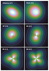 |
Fig. 1. Example models exhibiting the effect of the different shape parameters. Shown are an elliptical model (top left), a slosh model (top right), an M1 model (centre left), an M2 model (centre right), an M3 model (bottom left), and an M4 model (bottom right). For the models, we used an angle of θ = 30deg. The numeric values show the magnitude of the respective parameter. |
![Mathematical equation: $$ \begin{aligned} S^{\prime }(x, y) = S(\{\epsilon [x \cos \theta _0 - y\sin \theta _0]^2 + [x\sin \theta _0 + y\cos \theta _0]^2/\epsilon \}^{1/2}), \end{aligned} $$](/articles/aa/full_html/2025/03/aa52618-24/aa52618-24-eq18.gif) (17)
(17)
where S(r) is the original radial surface brightness and θ0 is the inclination angle of ellipse (between 0 and 180deg). The radial surface brightness was parametrised in the same way as for the standard profile analysis. As is standard when modelling clusters with MBProj2D, observational effects such as PSF and background were also accounted for by the model and uncertainties were calculated from the MCMC chain.
We note that the ellipticity parameter can describe clusters which are likely physically unrealistic (where ϵ ≲ 0.2). Informative, rather than flat, priors could be useful for a future analysis. The eccentricity parameter might be better than ellipticity, as its parameter space is biased towards more circular objects.
2.11. Slosh
Slosh (H) is a new parameter we designed to model how asymmetric the surface brightness is about the cluster. It has the appearance of the gas sloshing in the potential well of the cluster, as is thought to be the origin of cold fronts (see Markevitch & Vikhlinin 2007). As with ellipticity, we modelled this within MBProj2D as a modification to the projected surface model brightness. Similarly, an example model with slosh is shown in Fig. 1.
The projected surface brightness on the sky, S′, at a radius r and angle θ, is
![Mathematical equation: $$ \begin{aligned} S^{\prime }(r,\theta ) = A(H) \, S(r[1+H \cos (\theta +\theta _0)]), \end{aligned} $$](/articles/aa/full_html/2025/03/aa52618-24/aa52618-24-eq19.gif) (18)
(18)
where the slosh factor, H, lies between zero and one, S(r) is the original symmetric distribution and θ0 is the sloshing angle (between 0 and 360deg). As H tends towards zero, the distribution becomes the original symmetric one, while values of one give an extreme asymmetric distribution. Here, A(H) is a factor to ensure that the total brightness of the cluster model is not modified by changes in H. By considering the relative area of a circle with the slosh transformation applied, compared to its original area, one finds that
 (19)
(19)
Within MBProj2D the surface brightness is computed more easily in Cartesian coordinates (x, y) around the cluster centre, where
![Mathematical equation: $$ \begin{aligned} S^{\prime }(x, y) = A(H) \, S([x^2+y^2]^{1/2} + H[x\cos \theta _0 - y\sin \theta _0]). \end{aligned} $$](/articles/aa/full_html/2025/03/aa52618-24/aa52618-24-eq21.gif) (20)
(20)
If there is significant disturbance of the cluster, the position of the centre is likely to be different from the outer regions or one obtained assuming the cluster is symmetric. As described in Sect. 3, the centre of the main cluster was left free in the analysis.
2.12. Multipole magnitude
Forward modelling of parameters has some advantages over values measured directly from images. For example, the PSF of the source and the background can be included within the modelling, and the parameter uncertainties obtained using MCMC. Therefore we created forward models of the cluster which include azimuthal variations similar to power ratios. The surface brightness of a symmetric model profile S(r) was modified to produce the following distribution:
![Mathematical equation: $$ \begin{aligned} S^{\prime }(r, \theta ) = [1 + M_m \sin (m \theta + \theta _0)] \, S(r), \end{aligned} $$](/articles/aa/full_html/2025/03/aa52618-24/aa52618-24-eq22.gif) (21)
(21)
where m is a multipole index, θ0 is an inclination angle that ranges from 0 to 360/mdeg, and Mm is the multipole magnitude that varies between zero and one. Images of models with these multipole variations are shown in Fig. 1. MBProj2D computes the model image in Cartesian coordinates before comparison with the data. Firstly, the pixel sky coordinates (x, y) are rotated on the sky in reverse around the cluster centre by θ0 to compute rotated coordinates (xr, yr). Using sin θ = yr/r and cos θ = xr/r, sin(mθ) is calculated using the standard multiple angle formulae. When r = 0, θ = 0 is used above.
In our analysis we computed the morphological parameters M1 to M4 by fitting the multipole model to the data. As can be seen by the images, the parameter M1 has a shape which is somewhat similar to the shape of a cluster with the slosh parameter (H) applied. This leads to a correlation between these parameters, particularly for objects with lower data quality. Parameter M2 also looks similar to an elliptical cluster (ϵ) and so these parameters are also correlated.
2.13. Test of new parameters
We tested our new morphological parameters on images of 83 galaxy clusters detected from South Pole Telescope (SPT) surveys (Bleem et al. 2015) using the Sunyaev-Zel’dovich (SZ) technique and observed by Chandra in the X-ray waveband (McDonald et al. 2013; Sanders et al. 2018). Section 3.4 describes these data and their analysis. These clusters show a wide variety of different morphologies and their images have high spatial resolution and good data quality. The data were analysed seven times, one for each of the morphological parameters ϵ, H, M1, M2, M3, and M4, and also for a spherical cluster.
Figure 2 shows a corner plot of the parameters for the clusters in the sample, revealing significant variation in these parameters between the clusters. Some parameters are clearly correlated with each other, including ϵ and M2, and M1 and H.
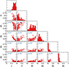 |
Fig. 2. Corner plot of the median MBProj2D shape parameters for Chandra observations of clusters in the SPT cluster sample. The quantities are plotted against each other, while the rightmost panels show the probability density of the values. The Pearson correlation coefficient is shown in each panel. |
The most distured clusters are found by selecting objects with more extreme values of these parameters. Fig. 3 shows SPT-CLJ0014-4952 has a strong slosh and M2 signal. SPT-CLJ0307-6225 has pronounced non-circular ϵ, H and M1. SPT-CLJ0304-4401 has a large M1, M2 and M3 signal because it has a triangular morphology. SPT-CLJ2342-5411 is elliptical, with large ϵ and M1 values. The modelling appears to perform well by picking up the disturbances that the human eye can see in the images. We further compare the Chandra and eRASS1 cluster results in Sect. 7.
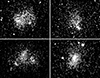 |
Fig. 3. Example Chandra images from the SPT sample shown in Fig. 2. Top left: SPT-CLJ0014-4952 [ϵ = 0.85, H = 0.50, M1 = 0.36, M2 = 0.26, M3 = 0.06, M4 = 0.03]. Top right: SPT-CLJ0307-6225 [ϵ = 0.58, H = 0.75, M1 = 0.88, M2 = 0.37, M3 = 0.27, M4 = 0.28]. Bottom left: SPT-CLJ0304-4401 [ϵ = 0.75, H = 0.14, M1 = 0.64, M2 = 0.26, M3 = 0.33, M4 = 0.11]. Bottom right: SPT-CLJ2342-5411 [ϵ = 0.64, H = 0.08, M1 = 0.71, M2 = 0.38, M3 = 0.07, M4 = 0.07]. |
3. Data analysis
3.1. Introduction
The inputs of our analysis were created using the same pipeline as in B24, although we only used the monochromatic X-ray images in a band of 0.2–2.3 keV. We only took data from the cameras without a light leak (i.e. the so-called TM8 data which combines data from telescope modules, TMs, 1, 2, 3, 4, and 6). These images and exposure maps were produced using the standard eSASS analysis software (Brunner et al. 2022), version eSASSusers_211214_0_4, which is equivalent to the publicly available version eSASS4DR1. We assumed that the clusters lie at the best redshift from the cluster catalogue. For those parameters which assume a value of R500, we took this from the cluster catalogue. The best fitting positions, for consistency, came from our MBProj2D analysis assuming a radially symmetric model, and are not necessarily the same as in B24.
3.2. MBProj2D analyses
Several of the parameters resulted from modelling the cluster with MBProj2D. For these analyses, we followed a common procedure which we describe here. As we only fitted monochromatic images, we assumed isothermal temperature profiles fixed to the median temperature from the MCMC chain obtained by B24 and used the Galactic absorbing column density from the catalogue.
The cluster profiles in B24 use a fairly strong prior on the inner density slope model parameter, α. This leads to some bias on the central slope measurement and concentration. Therefore, we re-analysed the cluster images using a density model with a weak prior on α (Table 2). As discussed by Käfer et al. (2019), clusters typically follow a β model with β = 2/3 in the outskirts, provided the core is otherwise modelled. The data quality in the eRASS1 survey also limits how sophisticated a model can be fitted to the data. Therefore, we used a simplified form for the density profile of Vikhlinin et al. (2009), compared to B24. We allowed β, the standard β-model outer slope, to vary over a more restricted range around β = 2/3 using a prior. The assumption of β = 2/3 could bias results in objects which deviate from that (e.g. flatter profiles in groups, see for example Johnson et al. 2009), although those parameters which depend on the density profile are sensitive to the central density. We did not allow the outermost slope in the parametrisation to vary and thus fixed ϵ to 0 and froze rs. The second β component was also not included in the model. The fitted profile was therefore a β model with an inner power-law core of the form
Priors on the MBProj2D analyses with the different models.
![Mathematical equation: $$ \begin{aligned} n_e^2 = n_0^2 \frac{(r/r_c)^\alpha }{[1+(r/r_c)^2]^{3\beta -\alpha /2}}, \end{aligned} $$](/articles/aa/full_html/2025/03/aa52618-24/aa52618-24-eq23.gif) (22)
(22)
where n0 is the central density and rc is the core radius. We note that due to the definition being density-squared, α here is twice the inner density slope and is not the same as the cluster density inner slope morphological parameter, α.
The input images used the same masking and sizes as B24. If a point source was fitted for in B24, we fitted for it here. Unlike B24, we only used monochromatic 0.2–2.3 keV band input images and used a fixed 4 arcsec bin size to ensure the best resolution. As our PSF, we took the standard eROSITA calibration 1.486 keV survey-averaged PSF, but averaged it in radius to make it symmetric. Signal outside 4 arcmin radius was also removed to match the definition of the eROSITA ancillary response matrices.
As in B24, we assumed that the sky background is flat across the fields examined. As most of the background in this energy band is due to X-ray sources, rather than noise intrinsic to the detector, we multiplied this background by the vignetted exposure map. Faint point sources with ML_RATE < 0.4 in the 0.2–2.3 keV band were masked out in the fit, while brighter ones were fitted as part of the model. If there were other clusters within the fitted image, these were included separately in the model. The position of the main cluster was allowed to vary in the MCMC analysis, while point source positions and positions of other clusters were fixed at their best fitting values.
MBProj2D was run with a standard spherically symmetric cluster model. We fitted the model to the data to obtain the best fitting, maximum-likelihood parameters. We then conducted an MCMC analysis to obtain chains of parameters. As described in Sect. 2, these chains were processed to calculate a random subset of density profiles. From these profiles, the distributions of the central density, inner density slope (cuspiness), and concentration were calculated. The resulting distributions were then used to compute the median values and 1σ percentiles. The median cluster position in the chain was used as the ‘best fitting’ cluster position and used to derive F.
For the shape parameters, ϵ, H, M1, M2, and M3, we repeated the fits to the data using MBProj2D, but we allowed the shape parameters to vary. In these analyses, we took the best fitting model from the above symmetric fit, added new free parameters which vary the morphology, then refit the data. Rather than give the median parameter values from the chain for the shape parameters or angles (which tend to 0.5 for the shape parameters with low counts), we provide the maximum-likelihood values, but computed the uncertainties using the MCMC distribution about the best fit.
We also repeated the first MBProj2D analysis with a fixed cluster peak position. The peak was computed from a Gaussian smoothed image of the cluster (see Sect. 2.5). The fit started from the previous best fitting parameters and the analysis was identical, except for freezing the main cluster position to the location of its peak.
3.3. Image-derived parameters
Several parameters were derived directly from the X-ray images rather than fitting models. Power ratios, the Gini coefficient, and centroid shift calculations require input images that do not contain point sources or neighbouring clusters. Therefore, for these measurements, we need to ‘fill’ in the regions occupied by these neighbouring sources. The photon asymmetry parameter, however, was derived with these regions masked out.
All these images initially require a mask. Firstly we computed a model of the sky from the best fitting radially symmetric MBProj2D model, including the effect of the PSF, but not background. We masked out regions where neighbouring clusters or point sources were at most half the contribution of the main cluster. In addition we masked out regions where these objects were more than 1/10 of the background level.
To make the filled input images where these masked regions were replaced, we computed the best fitting model of the main cluster and background from the MBProj2D analysis, including PSF, and computed a Poisson realisation of this. The regions which were masked out in the input image were replaced by this simulated image.
3.4. South Pole Telescope cluster data analysis
For comparison with the eROSITA clusters, we studied a subset of SPT-detected clusters (Bleem et al. 2015), observed in X-rays using Chandra and previously analysed in Sanders et al. (2018). For the Chandra analysis we used the same X-ray data and X-ray bands as described in Sanders et al. (2018). However, we used MBProj2D rather than MBProj2 as described in that paper and therefore fitted images rather than profiles.
The results for these clusters are compared with both the standard eRASS1 processing and those obtained from deeper eRASS:4 data. To make a better comparison for the eRASS:4 data we used very similar analysis procedures for both Chandra and the deeper eROSITA data. These data and procedures are close to those described in B24 for the eROSITA-Chandra flux comparison. We used a very similar mask for both datasets, where the cluster is masked beyond a radius of 5 Mpc and outer point sources outside a radius of 3 arcmin from the cluster core were excluded with a mask size with a minimum of 0.5 arcmin radius. The eRASS:4 eROSITA data were masked where they were outside of the field of view of the Chandra data. In the inner part of the cluster, due to the high spatial resolution, the point sources were masked for the Chandra analysis, while the sources are modelled within MBProj2D for the eROSITA data with the positions fixed from Chandra values. The Chandra data were binned to a spatial resolution of 4 pixels (2 arcsec), while we used the standard eROSITA spatial binning.
For both analyses, the clusters were assumed to be isothermal. When analysing the density profile for the symmetric cluster profile case for Chandra, we fitted multiple energy bands in order to constrain the cluster temperature. The Chandra background in each energy band was assumed to have the shape of the standard blank sky background, but with a variable log normalisation factor.
For eROSITA we fitted monochromatic 0.2–2.3 keV TM8 images of the clusters, but fixed the temperature to the median value obtained by Chandra. The centre of the cluster was fixed to the Chandra peak. When studying the morphological parameters which affect the shape of the cluster (see Sect. 2.13), we fitted a single band Chandra image in the band 0.5–4.0 keV, again fixing the temperature at the value obtained from the multi-band fit.
For both eRASS:4 and Chandra we assumed the same density parametrisation as for our eRASS1 analysis, with the same priors on the parameters. The metallicity was fixed to be 0.3 solar, as for the eRASS1 analysis.
4. Cluster simulations
To better understand our results we undertook simplified simulations of clusters on the eROSITA sky. The main aim of these simulations was to investigate the parameter biases due to the measurement process and the quality of data. In addition we wanted to check whether cluster morphology can have a significant affect on the eROSITA selection function.
Rather than making a full eROSITA simulation of the whole sky (Comparat et al. 2020; Seppi et al. 2022) we made simulations of individual clusters at random positions on the eROSITA sky and attempted to detect and measure their properties. The clusters were assigned luminosities and redshifts from a grid, with 9 logarithmic-spaced values of L500 between 1043 and 1045 erg s−1 and redshift values of 0.02, 0.035, 0.05, 0.07, 0.1, 0.15, 0.2, 0.3, 0.4, 0.5, 0.6, 0.7, 0.8, 1.0, and 1.2. Using the covariance matrix method described in Comparat et al. (2020), we generated random cluster masses, temperatures, and profiles. Clusters were assigned to a grid point by generating a mass function for the relevant redshift and assigning randomly generated clusters nearby in mass and redshift. Those clusters with luminosities close to the grid point value were assigned to it.
To make the simulated image of a randomly selected cluster for the grid point, we used MBProj2D to generate a model image for the cluster given its density profile, temperature, and Galactic absorption. The images were created in the band 0.2–2.3 keV, with a dimension of 70 arcmin for z = 0.02, 60 arcmin for z = 0.035, 50 arcmin for z = 0.05, and 40 arcmin otherwise. The cluster location was chosen randomly to lie within the region of sky that the cluster sample was obtained from in B24. The image was convolved with the eROSITA PSF and multiplied by the eROSITA eRASS1 exposure map at that sky position. Wavelet filtered maps of the eROSITA sky were used as a background, where structures below scales of around 30 arcmin were removed. No AGN were included in the simulations. We split the eROSITA TMs into two sets (TMs 5 and 7, and the rest), which were simulated separately. Poisson realisations of the two sets of model images were created. The summed image of the two sets of TMs was used for detection, while only the one excluding TMs 5 and 7 was used for characterisation.
To tell whether a cluster would be detected, we applied the eSASS pipeline to the simulated image. Initially, erbox was used on the simulated image to make a list of sources (with likemin=6, nruns=3, boxsize=4, and bkima_flag=N). This source list was supplied to erbackmap to make an initial background map (using scut=0.00005, mlmin=6, maxcut=0.5, smoothval=15, snr=40, and smoothmax=360). erbox was run a second time using the background map (with likemin=4 and bkima_flag=Y). We run erbackmap a second time to produce a new background map based on the generated source list. erbox was run again using the previous background map and a new background map was generated using erbackmap. We then ran the maximum-likelihood source detection based on the previous source list, using ermldet with parameters likemin=5, extlikemin=3, cutrad=15, multrad=15, extmin=2, extmax=15, nmaxfit=4, nmulsou=2, shapelet_flag=no, and photon_flag=no. These parameters are the same as used for the main eROSITA catalogue. A cluster was detected if there was an object in the output catalogue with non-zero extent within 2 arcmin of the input position.
One of the major differences between this simplified detection pipeline and the standard one is that we used image based rather than photon based detection. Photon based detection uses a separate PSF for each photon, making use of smaller PSF at the centre of the telescopes relative to the outskirts as sources scan across the field of view. Image based detection uses an average survey PSF and is significantly faster, but should be less sensitive close to the detection threshold.
The detected clusters were analysed in a very similar way to the real clusters. The images of the clusters, excluding TMs 5 and 7, were analysed with the MBProj2D and image based routines. The background component was assumed to have a flat count rate over the 40 arcmin region. To obtain the density-based parameters, such as concentration, we fitted a Vikhlinin model using MBProj2D with the same priors as used for the real data here. Rather than run a full MCMC analysis for each simulated cluster, we just found the maximum-likelihood parameters. The forward-modelled shape parameters (ϵ, H, M1, M2, M3, and M4) were obtained by fitting in MBProj2D using the same density profile priors as for the density analysis. We note that the centre of the cluster was allowed to be free during these fits. The power ratios, photon asymmetry, centroid shift, and Gini parameters were calculated from the simulated X-ray image but assuming the input R500 rather than determining it from the data.
In our input models, we simulated a variety of cluster shapes, including spherical, elliptical (with ϵ = 0.7), sloshed (with H = 0.3), or with M1, M2, M3, or M4 equal to 0.3. This allowed us to test our ability to recover the input parameter shape values or examine how cluster shape affects the obtained image-based parameters (such as power ratios or photon asymmetry).
5. Results
In this section we present the morphological parameters obtained from the real eROSITA cluster sample. Detailed information about the catalogue is given in Appendix A. In Fig. 4 we plot each of the parameters against the redshift of the source. For this plot we split the clusters into two subsamples (Table 3). The first is a bright subsample of clusters, where there are more than 300 counts in an 800 kpc radius aperture and the number of counts is greater than three times the lower uncertainty on the number of counts. For these points we colour markers using the X-ray luminosity within the 800 kpc aperture and show the uncertainties on the values. A fainter subsample with at least 25 significant counts are plotted with smaller markers.
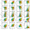 |
Fig. 4. Morphological parameters against redshift. The parameters are plotted for the bright cluster subset (≥300 counts) with larger markers. The small markers show clusters with at least 25 counts, without plotting uncertainties. The colour scale shows the X-ray luminosity (log erg s−1 in the 0.2–2.3 keV band) inside an aperture of radius 800 kpc. The parameters are the central scaled gas density (ns, 0), central electron density (n50), concentration from 80–800 kpc (c80 − 800), concentration from 0.1R500 to R500 (c500), central density slope (α), slope at fixed radius (α50), ellipticity (ϵ), slosh (H), multiple magnitudes (M1 to M4), power ratios (P10 to P40), photon asymmetry (Aphot), centroid shift (w), Gini coefficient (G), and fit-peak offset (F). |
eRASS1 cluster subsamples.
Figure 5 shows the parameters plotted as a function of the number of counts in the cluster, computed within an aperture of 800 kpc. As some of our measurements are sensitive to the quality of the data, this plot is ideal for identifying biases due to this. The colour scale indicates the redshift of the cluster. The same results are plotted in Fig. 6, but showing them as a function of X-ray luminosity within an aperture of 800 kpc. The colour scale in this figure shows the redshift of the clusters.
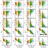 |
Fig. 5. Parameters against number of counts in an 800 kpc aperture. These parameters are plotted for the bright cluster subset (≥300 counts) with larger markers. The small markers show clusters with at least 25 counts, without plotting uncertainties. The colour scale shows the cluster redshift. |
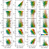 |
Fig. 6. Parameters against X-ray luminosity. These parameters are plotted for the bright cluster subset (≥300 counts) with larger markers. The small markers show clusters with at least 25 counts, without plotting uncertainties. The X-ray luminosity is inside an 800 kpc radius aperture in the 0.2–2.3 keV band. The colour scale shows the cluster redshift. |
Plotting the parameters as a function of the number of counts, we see that many of them are clearly increasingly biased towards the low count regime. This is particularly true for those parameters which are not based on the MBProj2D forward modelling method (e.g. power ratios and photon asymmetry). In addition we see that when plotting these values as a function of luminosity, the clusters are clearly separated in redshift for these parameters. The same parameters are also separated as a function of luminosity, if plotted as a function of redshift.
In theory, it could be possible that there are intrinsically strong variations in these parameters as a function of redshift and luminosity. However, in Sect. 6.8 our simulations show that these strong variations with luminosity and redshift (and therefore counts) are what is expected based on the level of noise in the survey and the PSF size.
The density parameters show increasingly higher values for more luminous or higher redshift clusters. However, there is no clear evolution with the number of counts. The scaled central density shows a weaker evolution than the physical density at fixed radius. The concentration parameters do not show any clear evolution with redshift of luminosity. For the shape parameters, ϵ, H, and M1 to M4, the results become roughly randomly distributed in the lower count regime below 100–200 counts.
Similarly to the Chandra observed SPT sample (Fig. 2) we plot a corner plot of the various shape parameters. Figure 7 shows the parameters ϵ, H, M1, M2, M3, and M4 for the subset of the brightest clusters (≥300 counts). The parameters show a very similar distribution to the SPT sample results, although they are noisier due to the lower number of counts. We observed that some of the parameters are correlated with each other, such as for Chandra, with ϵ and M2 being inversely correlated and H and M1 correlated.
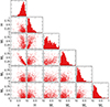 |
Fig. 7. Corner plot of the median MBProj2D shape parameters for the bright cluster (≥300 count) subset. The quantities are plotted against each other, while the rightmost panels show the probability density distribution of each value. |
In Fig. 8 we show a correlation matrix between the various parameters for a subset of bright clusters. We only include the bright clusters, as the parameters become noise dominated when a cluster is faint, leading to a reduction in any correlation. In this plot we also include the peak and best fit versions of those parameters when appropriate. It can be seen that there are generally strong correlations between a high central density, concentration and central slope. There are some weaker correlations between  and the central slope and concentrations, compared to n50. The concentrations measured in physical or scaled apertures, or measured around the peak and best fit positions are all strongly correlated.
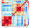 |
Fig. 8. Correlation matrix between different parameters for the bright cluster subset. Values were measured for clusters with more than 300 counts to reduce the effect of the statistical errors. Log values were taken for the photon asymmetry, power ratios and centroid shift. We also show the correlation with log cluster luminosity (L500), log number of counts in R500 (cts500), and log redshift. |
There is some mild correlation between the ellipticity (noting that higher ellipticities are rounder clusters) and the central density and concentration. The parameters H, M1 to M4, power ratios, F, and w are generally inversely correlated with the central density, concentration and central slope. The ellipticity and M2 are strongly inversely correlated, while H and M1 show correlation. The Gini coefficient is correlated with central density, concentration and inner slope. Several of the parameters measured from images (power ratios, photon asymmetry and centroid shift) are negatively correlated with the number of counts (see Sect. 6.8).
In Fig. 9 we show example brighter clusters with a similar number of counts, showing a diversity of morphology. Examples include a cluster with a high concentration and central density (1eRASS J124009.9-482612) and another with low concentration and central density (1eRASS J124116.4+183310). Elliptical clusters (low ϵ) include 1eRASS J043817.8-541917, 1eRASS J053128.2-751032, and 1eRASS J124116.4+183310, while 1eRASS J124009.9-482612 has a low ellipticity. The elliptical clusters generally have larger M2 values. 1eRASS J043817.8-541917 has a high slosh (H) because of its offset central peak and similarly with 1eRASS J053128.2-751032, 1eRASS J055252.8-210407, 1eRASS J124116.4+183310, and 1eRASS J224956.6-642532 has a large M1 value. 1eRASS J224956.6-642532 has the largest M3 value because there is bright triangular shape feature around the central peak. 1eRASS J051016.7-451911, 1eRASS J124009.9-482612, and 1eRASS J124116.4+183310 have the largest M4 values in this subsample. Those clusters with the largest peak-fit offsets are 1eRASS J051636.6-543031, 1eRASS J053128.2-751032 and 1eRASS J124116.4+183310, while 1eRASS J124009.9-482612, 1eRASS J140755.5-505938, and 1eRASS J155821.9-140957 show small offsets.
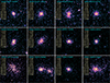 |
Fig. 9. Example cluster images and morphological parameters. The clusters chosen are those from the catalogue with between 920 and 1080 counts within 800 kpc radius and an uncertainty on the number of counts of less than 5%. The exposure-corrected images are in the 0.2–2.3 keV band with the same angular scale and have been smoothed by a Gaussian with σ = 8 arcsec. We show the cluster name, redshift, scaled central density (ns, 0), concentration (c80 − 800), ellipticity (ϵ), slosh (H), multipole magnitudes (M1 to M4), and peak-fit offset (F). |
Although for the most disturbed appearing clusters (e.g. 1eRASS J124116.4+183310) several of the parameters indicate their disturbance, there are cases where only one or a few of the parameters indicates some disturbance (e.g. 1eRASS J124009.9-482612). One interesting example is J043817.8-541917, where visual inspection would likely miss the disturbance-indicating values of ϵ, H, M1, M2, and M3.
6. Parameter biases
6.1. Introduction
There are several biases which can affect the obtained parameters. It is important to understand these biases before using the parameters blindly, as they can be a function of other cluster properties. For example, some parameters show strong evolution with redshift or luminosity with no change in cluster morphology. The morphology of the cluster can also affect how likely it is to be selected, presenting a biased subset of clusters with respect to certain characteristics. We summarise the various biases in Table 4.
Potential biases.
6.2. Morphological detection bias
The morphology of a cluster may affect how easy it is for a cluster to be detected in the X-ray waveband. For example, cool core clusters are known to have higher luminosities for the same mass compared to non-cool core clusters (e.g. Edge & Stewart 1991; Pratt et al. 2009; Hudson et al. 2010; Mittal et al. 2011). Clusters with disturbed morphologies are known to have lower luminosities. Therefore, for a fixed detection threshold it may be easier to detect cool core clusters and less easy to detect disturbed clusters (Eckert et al. 2011), although there are methods which can reduce this bias (e.g. Käfer et al. 2020). However, as a result of the PSF fitting maximum likelihood detection approach used to make the eROSITA catalogues, there may be objects in which the cool core makes the cluster more likely to be detected as a point source and missed in the cluster catalogue (e.g. Bulbul et al. 2022), particularly towards higher redshift where the PSF is more important. At low redshifts the PSF fitting detection method may miss objects which have flat cores in surface brightness, particularly if the core size becomes larger than the fitting radius (Xu et al. 2022). Large groups or clusters with flat cores may be confused with background variations. This bias will not change the parameters for an individual object, but as cool core clusters are more regular, the parameters obtained for the population near the flux detection limit or towards higher redshift may be biased by this effect.
The easiest to measure indicator of a cool core is the surface brightness concentration of a cluster. Cool cores also have higher central densities than non cool core clusters and steeper inner surface brightness profiles. In the eROSITA detection pipeline (Merloni et al. 2024), the significance of sources is measured by two parameters, firstly the detection likelihood (ℒdet; DET_LIKE_0 in the catalogue) and secondly the likelihood for the source to be extended (ℒext; EXT_LIKE in the catalogue). When computing the extension likelihood, the source is parametrised as a β-model with β = 2/3 and a variable extent.
Figure 10 shows these parameters for the whole cluster sample, as a function of the cluster detection likelihood or extension likelihood, and the total number of counts in the cluster in an 800 kpc aperture. It can be seen that for a fixed number of counts in a cluster, those with a higher detection likelihood have a higher concentration, a more dense core and a steeper density slope. For a fixed detection likelihood, those with the fewest counts are more concentrated, more dense and have steeper profiles. The pattern of extension likelihood is less clear. A selection in count space is less affected by the cluster morphology, particular above the threshold of ∼40 counts.
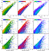 |
Fig. 10. Relationship between detection likelihood (ℒdet), extension likelihood (ℒext), counts, and morphological parameters. (Top panels) The median value of the concentration (c80 − 800; left), central scaled density (ns, 0; centre), and central slope (α; right), in grid points of ℒext and ℒdet. (Bottom panels) The median morphological parameter values for grid points of counts in an 800 kpc aperture and ℒdet or ℒext. |
The effect of concentration on selection is shown in further detail in Fig. 11, where the cumulative distribution of concentration is shown for subsamples with different cuts on exposure, counts, detection likelihood and extension likelihood. The effect of increased exposure time is to reduce the peak of the distribution to lower values of c500, but the distribution of c80 − 800 is relatively unchanged. Lower numbers of counts is associated with larger values of both concentration values, although above 80 counts, the distributions do not change further. Increasing the detection likelihood threshold leads to distributions of c500 with a peak at higher values, but a narrower width. The effect of ℒdet on c80 − 800 is mostly to narrow the distribution peak. The effect of extension likelihood cuts on c500 is less clear, with low and high extension likelihoods showing a peak at higher values. For c80 − 800, higher ℒext thresholds lead typically to lower concentration values, although this effect seems to saturate near values of around 12. We also note that for the low count regime, the distributions will be broadened out due to statistical noise.
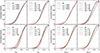 |
Fig. 11. Cumulative distribution of concentration for different subsamples of the eRASS1 catalogue. The cumulative distributions are shown as a function of exposure time (texp), number of counts in a 800 kpc aperture, detection likelihood (ℒdet), and extension likelihood (ℒext). The left panels show the distribution of c500, while the right panels show the distribution of c80 − 800. |
We measured concentration with apertures with angular sizes that vary with redshift, and for c500 also vary with mass. Choosing different cluster susbsamples, for example according to exposure time, will select clusters with different redshift and mass distributions. Therefore, the interactions between how likely a cluster is detected, concentration, exposure time, number of counts, and detection threshold cuts are rather complex. However, it might be noted that the maximum shift for the median concentration is 0.2 dex for c80 − 800 between the high and low count cluster subsamples.
We examined the effect of concentration on selection in more detail with the aid of simulations. Figure 12 shows the fraction of clusters detected as a function of concentration at different redshifts and luminosities. However, we note that the concentration in this plot is that computed from the input and not from the reconstructed profiles. It can be seen at the lowest redshifts bins we would not detect groups or clusters if they have a flat surface brightness profiles (c80 − 800 ≲ −1). The effect is stronger for the less luminous (fainter) objects. This is likely due to the fixed size of the detection aperture and the background map generation process.
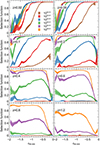 |
Fig. 12. Selection function of clusters with different redshifts and luminosities as a function of concentration that were calculated from simulated observations of spherical clusters. The panels show the detected fraction of clusters at different redshift. For each redshift, we show the detection fraction as a function of concentration for different luminosities (erg s−1). The log concentration (c80 − 800) is computed from the input model profile and is binned into bins of 0.1 width. |
At higher redshifts we would not detect clusters if they have very concentrated surface brightnesses, for example due to a cool core. At a redshift of 0.4, clusters with c80 − 800 ≳ −0.2 (or around 60% of their flux within 80 kpc) are lost, even if they have luminosities as high as 1045 erg s−1 (roughly a 1015 M⊙ cluster). This threshold reduces to −0.4 at z = 0.6, −0.5 at z = 0.8 and −0.6 at z = 1.2 (with 25% of their flux within 80 kpc). For the SPT-selected clusters observed by Chandra (Sect. 3.4), we found 4% of objects have c80 − 800 ≳ −0.4, 9% are at value greater than −0.5 and 13% greater than −0.6. This selection effect is due to these objects becoming more point-like and the eSASS detection pipeline not detecting the extension of the object, because of a low extension likelihood. Therefore, extreme cool core objects at high redshifts may be missing from the cluster sample. One example is the extreme cool core Phoenix cluster (McDonald et al. 2012), which is not detected as an extended source in the eRASS1 catalogue (also see Bulbul et al. 2022).
The selection effect seen above can also be seen in observed clusters by plotting the average cluster luminosity as a function of redshift in bins of concentration (Fig. 13). At lower redshift the least luminous clusters are the most concentrated. Clusters with similar luminosities but flatter cores would not be detected by the source detection. The opposite effect is present at high redshifts for c500, where the least luminous clusters have the flattest cores, as peaked clusters that look similar to point sources are not detected as extended clusters.
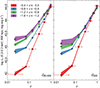 |
Fig. 13. Median X-ray luminosity of clusters in bins of concentration. The left panel uses bins of c80 − 800, while the right panel shows c500. The uncertainties shown are calculated with bootstrap resampling. All eRASS1 clusters are included in this analysis. |
6.3. Cool core mass and radius bias
Parameters measured at or within radii scaled with R500 are sensitive to the accuracy of that measurement. Cool core clusters have high central gas densities and therefore X-ray bright cores. As the cluster mass and radius is obtained using the cluster luminosity in the eRASS1 cluster catalogue, the presence of a cool core can bias the cluster radius and parameters which are measured at a scaled radius. A cool core will increase the cluster luminosity and R500, leading to a measurement at fixed scale radius being measured at a higher physical radius than expected. However, the cluster radius only scales weakly with the mass with a one-third power. In cool core clusters, ns, 0, will be reduced by this effect. Similarly, non-cool core clusters may have boosted central densities, although the effect will be smaller, as they have a flat core in their density profile.
Many of the parameters are affected by this bias in radius determination including ns, 0, α, c500, power ratios, w, and Aphot. Parameters unaffected include n50, c80 − 800, ϵ, H, and multipole magnitudes. Those parameters which are affected by this issue are indicated in Table 1. For example, if we artificially increase R500 by 10%, the median c500 increases by 0.035, c500* by 0.026, ns, 0 by −0.022, ns, 0* by −0.036, α by 0.038, and α* by 0.033. Similar changes in the opposite direction are seen if R500 is decreased by 10%.
6.4. Position bias
The central positions of our clusters are determined by the fitting of a model for the surface brightness to an image. For those parameters obtained using MBProj2D, the central cluster position was allowed to vary during the analysis, while other clusters and modelled point sources in the field were frozen at their best fit location. For those parameters not measured using MBProj2D, we used the median chain value from the MBProj2D symmetric modelling as the cluster centre. Some of these positions can differ from the standard cluster catalogue location, due to the slightly different modelling procedure. The cluster positions obtained from the MBProj2D analyses are the locations of the centre of the model which fit the cluster best overall, in a statistical manner.
As stated previously, for some parameters where the choice of centre makes a difference, we provide fitted centre and peak centre values. Figure 14 shows average quantities in bins of offset between the peak and best fitting positions (F). The central density parameters, concentration, central slope, photon asymmetry, and power ratio P10 are all significantly different if there is an offset between the peak and best fitting positions. We also see lower dispersions for some quantities when using the peak position.
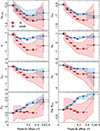 |
Fig. 14. Fit-centred and peak-centred (∗) quantities as a function of the distance between the cluster peak and the best fit position for a cluster subsample with ℒext > 6 and ℒdet > 20. The median quantities in bins of F are shown with bootstrap resampling uncertainties. The shaded regions show the 1σ percentile width of the data points within each bin. |
For the MBProj2D-derived shape parameters, the cluster centre was also allowed to be free in the analysis. For parameters ϵ, H, and M1 the size of the offset between the standard fit position and the one with varying 2D shape is clearly correlated with the shape parameter. At more extreme parameter values, this shift can be 0.1 to 0.2R500.
6.5. Point spread function bias
When looking at objects towards higher redshifts (or more precisely, angular diameter distance) or lower masses, the finite size of the PSF of eROSITA becomes increasingly important and makes it harder to measure morphological parameters. Those quantities measured using the forward-modelling procedure of MBProj2D already take account of the PSF. For more distant objects, the uncertainties on the measured parameters grow due to the increased importance of the PSF size, but there should be no bias on the measured parameters if the functional form of the fitted profile is realistic (however, see Sect. 6.6).
There are several parameters, however, that do not consider the PSF in their determination. These include power ratios, w, Aphot, and G. Clusters at increasing distances with the same degree of disturbance will look less disturbed with these parameters, as the structure is smoothed out. In Sect. 6.8 we present the intrinsic variations of these parameters due to both the effects of noise and the PSF, as a function of redshift and luminosity.
6.6. Fixed parameter range bias
Some parameters, including ϵ, H, the multipole magnitudes, and G, are only defined for a range of zero to one. The definition of concentration restricts values to the range 0 to −2. In addition, for the very faintest clusters or most distant clusters, model priors may implicitly restrict the range on some of the forward-modelling obtained parameters.
The finite range means that as the uncertainty on a value increases, the obtained median values from an MCMC chain tend towards the centre of the allowed parameter range. If there is no constraint on a value, its 1σ error ranges, obtained from the 1σ percentiles of the chain will also tend towards encompassing 68% of the parameter range. For those parameters obtained using MCMC, the full posterior probability distribution can still be used as this effect increases, although model priors could become increasingly important.
To reduce this effect for the shape parameters, ϵ, H, and M1 to M4, rather than quoting the median chain value, we instead give the maximum likelihood value. The best fitting values are more evenly distributed over the parameter range when the number of counts is low, rather then being clustered around 0.5. This also makes comparisons with simulations easier, as we cannot run a full MCMC analysis on each simulation. Figure 5 shows that for objects with fewer than 200-300 counts, it is difficult to trust these individual shape parameters for single objects.
Using our simulations we also checked how well the fixed-range shape parameters can be recovered from the maximum likelihood fit. Figure 15 shows the range of parameter values obtained for the input cluster shapes given. At high luminosities and low redshifts, the input parameter can be recovered. Surprisingly, we found that the average best fit parameter does not tend towards the input parameter in the low count regime. The mean values tend towards an extreme (e.g. zero for ϵ and one for M1 to M4). The H parameter does not seem so badly affected by this bias. In these extreme cases seen in low photon count clusters, we found often the maximum likelihood model is a very elongated ellipse which passes through the brightest pixels. Therefore, one should take care if using the maximum likelihood values for these parameters from our catalogue of parameters in the very low count regime. The maximum likelihood parameters chosen for objects with low counts are obviously unphysical. In this case, an informative prior on these parameters could prevent these poor results, although this could make interpretation more difficult. More detail about the count range where this issue occurs is discussed in Sect. 6.12.
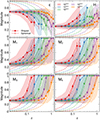 |
Fig. 15. Recovery of forward modelled parameters as a function of redshift and luminosity using maximum likelihood. The plots show the recovered parameter values as a function of redshift, for clusters with an input shape compared to an input spherical cluster. The error bar shows the average best fitting parameter and the uncertainty on the mean. The shaded region shows the 1σ range of the recovered best fitting parameters. The panels show shaped models with ϵ = 0.7, H = 0.3, M1 = 0.3, M2 = 0.3, M3 = 0.3, and M4 = 0.3, respectively, compared to the spherical models. |
6.7. Cluster shape affecting selection
In addition to how concentrated a cluster is, its 2D shape may affect whether it is selected as an extended source or not. The ermldet task assumes that a cluster has a symmetric shape with a β model profile.
In our simulations we tried to assess how much the cluster shape affects the likelihood that a cluster is selected as a function of redshift and luminosity. We computed this for a limited number of cluster shapes, including spherical, elliptical (ϵ = 0.7), sloshed (H = 0.3), first multipole (M1 = 0.3), and second multipole (M2 = 0.3).
Figure 16 shows the fraction detected for these different cluster shapes for different luminosities as a function of redshift. The results show that for these degrees of non-spherical morphology there are no significant changes in the detection efficiency of clusters. The largest effect seems to be for low luminosity objects at lower redshifts, where a slosh reduces the detection efficiency by ∼5%.
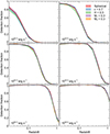 |
Fig. 16. Detection fraction as a function of redshift for different luminosities and shapes. |
6.8. Noise and distance
Several parameters do not take account of the PSF of the telescope. In addition, they may be affected by noise in the low count regime. Figure 17 shows measured non-forward-modelled morphological parameters for simulated clusters. Here we simulated spherical and shaped clusters with given luminosities and redshifts. The bands show the 1σ range of recovered properties as a function of redshift for the spherical clusters of different luminosity.
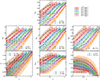 |
Fig. 17. Measured non-forward-modelled morphological parameters for simulated model clusters. Clusters are simulated with different luminosities and redshifts, after sampling from the mass function. The shaded region shows the 1σ range of recovered parameters of detected clusters simulated from spherical cluster models. The dotted and dashed lines show the median obtained parameters for non-spherical detected clusters with the parameters shown. |
It can be seen that for these parameters there are strong intrinsic variations with luminosity and redshift. As these clusters are completely symmetric, this is due to the increase in noise for fainter clusters and increased blurring for distant or less massive clusters. On the plots we also include the relations of the median for clusters with a shape given (one of H = 0.3, ϵ = 0.7, M1 = 0.3, M2 = 0.3, M3 = 0.3, and M4 = 0.3). For the brightest and nearest clusters we see a difference in the recovered parameters between the clusters with shape and the spherical clusters. However, we note that the Gini coefficient is primarily a measure of concentration, so we do not see a difference for the spherical and clusters with shape. Some parameters show little difference between spherical and non-spherical clusters, even for nearby luminous objects, such as P30 and P40.
6.9. Resolution bias
The more counts detected from a cluster in an annulus, the easier it is to measure properties at that radius. For example, to measure the central entropy of a cluster, one might, for example, create radial bins to measure a cluster profile and fit a model. The bins would need to be larger for poorer quality data, leading to a bias in the innermost regions. This could lead to a floor in the profile caused by the analysis method (see discussion in Panagoulia et al. 2014). Less bias would be present for clusters with more counts in the central region.
Our analysis method did not bin the data, so this should not be important above the pixel scale (although 4 arcsec pixels are 32 kpc at a redshift of 1). The error bars on a derived quantity should encompass the real value, unless the prior is unrealistic, or the parametric form is different from the real profile, leading to discrepancies in the outer parts of the profile driving the inner part.
6.10. Temperature and metallicity bias
We assumed that clusters are isothermal and have a 0.3 solar metallicity. If this is not the case, then density measurements or inner density slopes could be inaccurate. However, variations in temperature and metallicity would need to be strong to produce inaccurate densities, as the X-ray surface brightness is proportional to density-squared. One case in which they could become important is for groups, where the X-ray emission lines become dominant over bremsstrahlung emission for X-ray temperatures below around 1 keV. A substantial fraction of eROSITA clusters are lower mass objects with lower temperatures. Of those with temperature measurements, there are 550 objects with temperatures less than 1 keV and 2900 with temperatures less than 3 keV.
6.11. Unresolved point sources
Detected point sources are masked out in our analysis or simultaneously fitted. Due to the ∼30 arcsec survey PSF, its limited sensitivity and the source detection algorithm, we may miss point sources within clusters, or resolve parts of clusters as point sources. In addition, some fraction of clusters in the sample are contaminants, where single or multiple point sources could be confused to be extended sources. The purity of the main cluster catalogue is 86% (B24).
Unresolved point sources could give rise to artificial substructure within an object and so affect the morphological parameters. In addition, very peaked substructure could be detected as a point source and therefore removed. The strength of this effect could be redshift and luminosity-dependent. To better assess this in a future work would likely require the analysis of more realistic simulations incorporating a full range of cluster morphologies and source populations. Our existing simulations do not include point sources. If our simulations were to include a point source population, it would likely give rise to additional bias in the parameters, particularly in low luminosity and higher redshift objects.
6.12. Recovered parameter biases and uncertainties
Some of the listed biases affect whether a cluster is detected and others affect the measured parameters. Here we examine the combined effect of biases on the measured parameters using our simulations, ignoring selection effects. These simulations took account of the PSF, the data quality, the fixed parameter range and the choice of centre (fitted or peak), although point sources were not included. We also computed the statistical uncertainty of the parameters. These biases and uncertainties are studied as a function of redshift and number of cluster counts. Counts are more reliable than luminosity in predicting the data quality because it takes account of survey depth and absorption.
Figure 18 shows the difference between the recovered parameter value and its input. We emphasise that we are just using the median obtained parameter (or maximum likelihood in the case of the shape parameters) and do not include the probability density function for the parameter. For the density parameters, the input value was obtained by deprojecting the emissivity surface brightness profile (noting that this is not valid in all cases). For the shape parameters (ϵ, H and M1 to M4), we simulated clusters with known fixed parameter values and looked at the difference between the input and output. For the image based parameters (w, Aphot, and P10 to P40), we simulated spherical clusters and just plot the average value, noting that given perfect signal to noise the value should be −∞ in the log space used.
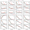 |
Fig. 18. Recovered parameter bias from simulated clusters as a function of the redshift and number of counts inside an 800 kpc radius circle. For the concentration, central density and cuspiness, shown is the difference between the recovered values and the input profile, after deprojecting the emissivity profile. For the shape parameters, ϵ, H and M1 to M4, we show the difference between the recovered and input values (0.7 for ϵ and 0.3 for the others), for simulations with non-spherical clusters. For the parameters w, Aphot and P10 to P40, we show the value for a spherical cluster. |
The largest biases are seen for fainter objects in the very lowest redshift bin, where the extent of the source means that the background level varies significantly over the region of the object. At these redshifts, the background level means that for the same number of counts the signal to noise ratio is lower. For higher redshifts, we see fairly moderate evolution in bias with redshift. The concentration measurements show some positive bias for low count clusters, although it is rather flat and small when there are more than 50–100 counts, except at very low redshifts. The peak centred concentrations show larger bias, although these simulated clusters are unrealistic by being perfectly spherical. The central density shows some bias of the order of 0.05–0.15 dex, although the sign and magnitude depends on whether the density at fixed radius is measured. Some positive bias in the central slope is seen, of between 0 and 0.5. For the shape parameters, there is some bias below 100 counts or so, due to the finite range of the parameter (Sect. 6.6). For the image based parameters, we see the same biases as seen in Fig. 17 and described in Sect. 6.8.
The uncertainties on the density profile parameters (Fig. 19) generally decrease with the number of counts and increase with redshift. There is not such a strong decrease in uncertainty on the central density with increasing counts if the peak position is used, which is likely because the central density is very sensitive to the central position and we are only using a subset of the data to determine this position. The statistical uncertainty on the cuspiness is generally large and redshift dependent. The forward-modelled shape parameters show declining uncertainties with increasing number of counts, and relatively little redshift evolution.
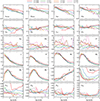 |
Fig. 19. Recovered statistical uncertainty in measured parameters from simulated clusters. This is the standard deviation on the difference between the input and recovered values, as in Fig. 18. |
7. Comparisons with previous results
7.1. Matched subsamples
To check for consistency, we compare the c500 concentrations and ns, 0 central densities for the same clusters with different analyses in Fig. 20. This comparison will be unaffected by selection effects. For three of these comparisons we computed using MCMC a median linear relation between eROSITA and the other values, assuming that the distribution is normal about the relation. We note that B24 report 15% lower fluxes in eROSITA first data release (DR1) processing compared to Chandra, which likely will give rise to a difference in central density of roughly half this value.
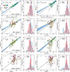 |
Fig. 20. Comparison of concentration and scaled central density measurements for the same cluster samples between eRASS and other measurements. The two left columns compare c500 and its distributions, while the two right columns show ns, 0. Median values are plotted as vertical lines. The number of counts for the cluster in the eRASS1 or eRASS:4 data is indicated by the colour. Top row: 66 Planck ESZ and eRASS1-detected clusters, with XMM-Newton results from Lovisari et al. (2017) and using the eRASS1 peak values. Second row: 66 SPT and eRASS1-detected clusters, analysed using Chandra data and taking the peak values from eRASS1. Third row: 83 SPT-detected clusters, extracting the values from Chandra eRASS:4 data using similar analysis procedures. Bottom row: 69 clusters detected in both eFEDS and eRASS1. The eFEDS survey results are from Ghirardini et al. (2022), while the eRASS1 results are the best fit position values. For the top three rows, we compute the best fitting linear relation between the results, assuming a normal distribution around the relation. |
The first comparison is to an XMM-Newton analysis of the Planck-detected early SZ (ESZ) sample (Lovisari et al. 2017). These clusters were matched to counterparts in the eRASS1 catalogue within a radius of 4 arcmin to make a jointly detected sample of 66 clusters, with a median eROSITA mass of M500 = 1014.92 M⊙. We note that the values of R500 used in the two analyses are different, which could lead to systematic differences, although R500 scales fairly weakly with mass. The cluster centres could also differ, although both used X-ray peak centres. Despite these possible differences, there is a reasonable agreement between the sets of concentrations, although there appears to be an offset increasing with lower concentration. The median cluster has a 0.1 dex higher concentration in eRASS1. If we examine the central density, there is scatter above the relation, which may be due to the assumed density profile form being too simple for these very bright clusters. There is evidence for a non-unity slope or offset between the relations, with low central densities for eROSITA found higher than XMM-Newton, and high central densities lower, although the small uncertainties on the bright objects are likely driving this fit. The median value, however, is exactly the same between the two sets of measurements for the same clusters. The differences between the two analyses could be the result of the R500 differences, background modelling, particularly due to the large field of view of eROSITA, point sources, and the differences in the assumed functional form of the density or surface brightness.
We also examined a sample of clusters detected by SPT (Bleem et al. 2015), in particular those previously studied in X-rays using Chandra by Sanders et al. (2018). We matched an eROSITA to SPT cluster if its distance is less than 4 arcmin, to make a sample of 66 objects, with a median eROSITA mass of M500 = 1014.14 M⊙. Section 3.4 describes the Chandra data analysis, which uses the same parametrisation for the density profile as for the eROSITA data. For both these analyses, we used the concentration as defined by the peak of the cluster. However, R500 for the Chandra analysis was from the SPT catalogue, while the eROSITA R500 was the value in the eRASS1 catalogue. The best fitting relation between eROSITA and Chandra is similar to the Planck clusters, with an increasing offset towards lower concentrations. The median cluster again shows a 0.1 dex higher concentration for eRASS1, although the median concentration is lower than for the Planck sample. For the central densities, again the median values are exactly the same between the two different sets of analyses. However, there is a similar non one-to-one relation found as with the Planck data, if fitting the datapoints.
In addition to matching the eRASS1 and Chandra SPT objects, we did a detailed analysis of eRASS:4 data for the whole Chandra SPT sample, using as similar a methodology as possible (see Sect. 3.4). In this case, we used the SPT R500 for both analyses and also studied objects which were not detected as clusters in eRASS1, producing a sample of 83 objects. The best fitting relation between the two sets of values is consistent with 1:1. The increased agreement compared to the eRASS1 sample is likely a combination of using exactly the same extraction regions and cluster centre and masking or modelling the same point source regions. However, the median cluster again shows a ∼0.1 dex higher concentration for eROSITA. The central densities show a good agreement between the two analyses, with a relation which is consistent with 1 : 1. The median density values are also very close to each other.
Finally, we compared two different eROSITA surveys, eRASS1 and the deeper eROSITA Final Equatorial-Depth Survey (eFEDS; Ghirardini et al. 2022), for clusters which match with a counterpart within 2 arcmin of the other survey, finding a sample of 69 objects. The median eROSITA DR1 mass of this sample is M500 = 1014.41 M⊙. eFEDS shows a rather narrower concentration distribution for the same clusters, with a median around 0.1 dex lower than eRASS1. The width of the concentration distribution is also narrower than the XMM and Chandra results, which may be due to the prior on the inner slope of the density parametrisation, α > 0, used by Ghirardini et al. (2022). The median central densities are similar for the two different analyses and datasets.
Overall, there is a reasonable agreement between the different analyses for the same cluster samples, considering that the datasets are different and some of the analyses are independent. However, there are suggestions for the analyses using the eRASS1 clusters combined with Planck ESZ or SPT, of an offset for the lowest concentration or lowest density objects. There is good agreement between the matched analysis procedures for the eRASS:4 and Chandra data. The scatter seen in the eRASS data is affected by the number of counts. Planck clusters are X-ray bright (mean in log space of 740 counts in eRASS1) compared to the SPT sample (log-space mean of 100 counts). The eFEDS sample is fainter than the SPT objects, with a log-space mean of 35 eRASS1 counts. The differences in the other comparisons could be due to different analysis procedures, the locations of the cluster centres, unresolved point sources in eRASS1, the spatial masks for the datasets, background modelling and the 15% offset in flux found in the DR1 processing (B24).
7.2. Whole samples
We also compared whole samples, although it must be noted that selection effects may dominate any differences between them. In Paper II we investigate the underlying distributions, taking account of selection effects. Figure 21 shows cumulative distributions of parameters for the Chandra observed SPT sample, the XMM-Newton observed Planck ESZ sample (Lovisari et al. 2017), and the eFEDS sample (Ghirardini et al. 2022). For eFEDS1, we show distributions of parameters for subsamples with increasing cuts on the detection likelihood. High detection likelihood objects are the most significant in the survey and have the smallest statistical uncertainties on the parameter values. For comparison with eFEDS, we also show an eRASS1 subsample with the same cuts in detection and extension likelihood and with a similar observation depth, although we do not match the background levels. Where appropriate, we also show the distributions for both the parameters measured with a free cluster centre and those measured where the peak position is used.
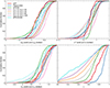 |
Fig. 21. Cumulative distribution of parameters for SPT, Planck ESZ, and eFEDS clusters compared to eRASS1 for different detection thresholds. For eROSITA the solid lines show the values fixing the cluster position at the peak, while the dotted lines show the distribution for when the cluster position varies during the fit. Shown are the concentration (top left), cuspiness (top right), central scaled density (bottom left), and ellipticity (bottom right). Planck values are taken from Lovisari et al. (2017) and eFEDS values are obtained by Ghirardini et al. (2022). The eFEDS-like curves are for eRASS1 clusters with ℒdet > 5, ℒext > 6 and an exposure time between 1000 and 1400s, to match eFEDS. The median published log masses of the SPT, Planck and eFEDS samples are 14.7, 14.8, and 14.0, respectively. The eROSITA sample median log M⊙ masses are 14.4, 14.5, 14.6, and 14.8, for detection likelihood thresholds of 20, 40, 80, and 320, respectively. |
We see that the SPT and Planck samples show similar distributions of concentration. eFEDS shows a median concentration close to the SPT value, although the wings are broader. The eRASS1 clusters have systematically higher concentrations than the other samples. The c500* values are larger than c500, as expected. The eRASS1 median concentration is around 0.3 dex larger than SPT or eFEDS medians. If we examine subsamples with larger ℒdet thresholds, the median shifts to higher concentration values, as previously seen in Fig. 11. However, as we discussed for Figs. 10 and 11, cuts in count space above ∼40 do not substantially change the concentration distribution.
The reason for the different concentration distribution for eRASS1 compared to the other surveys could be due to its X-ray selection and relatively shallow depth, although we note that there are differences in the measured parameters for the same clusters which could contribute (Sect. 7.1). X-ray selection is more sensitive to concentrated clusters (Sect. 6.2). Figure 11 also shows that increasing ℒext would not reduce the median concentration to bring it in agreement with the SZ-selected samples. Increasing the depth of the survey decreases the median concentration, although the effect is relatively modest up to 800s. Lovisari et al. (2017) give a median concentration for the REXCESS sample of representative X-ray selected clusters (Böhringer et al. 2007) as c500 ∼ −0.6, which is consistent with what we found for eRASS1 (Fig. 21).
eFEDS contains less concentrated clusters, despite its X-ray selection, which may be due to the survey depth. We check this using the ‘eFEDS-like’ eRASS1 subsample, noting that the eFEDS cluster positions are fitted for. Comparing the eFEDS-like concentrations when the central position is fitted for, we see a similar distribution to eFEDS. The cumulative fraction at the most and least concentrated peaks are very similar to eFEDS. However, eFEDS-like is more concentrated by around 0.1 dex at the median. This may be due to the difference in the fitting method, including the functional form used, or the average background level.
The median α* is similar to eFEDS, although eFEDS does not use peak cluster positions. The difference in slope between eFEDS and eFEDS-like is likely due to the positive central density slope prior used by Ghirardini et al. (2022) compared to the wide prior used here. The SPT and Planck clusters do not show such steep inner profiles, with median values around 0.25 smaller than eRASS1. Larger ℒdet thresholds increase α*, although the effect is small for modest increases.
The median central scaled densities in eRASS1 clusters with a lower detection threshold are similar to those found in the SPT and Planck clusters, although the central density for eRASS1 strongly increases with ℒdet. eFEDS clusters show a density distribution with a median reduced by around 0.3 dex from eRASS1 with ℒdet > 20. The differences between eFEDS and eFEDS-like is again likely affected by the different priors on the central density slope assumed in the analyses.
The raw ellipticity distribution for eRASS1 is dominated by measurement errors for lower detection thresholds. As the values can only lie between zero and one, and clusters are more circular than elliptical, values are biased low for low numbers of counts As the detection threshold increases, the distribution approaches the SPT distribution, with a median of ϵ = 0.77. eFEDS values are lower, but they also have significant measurement errors. It is unclear why the eFEDS and eFEDS-like samples show different ellipticity distributions. Planck clusters, show significantly larger ellipticity values, indicating they are more circular. However, we can compare directly the eRASS1 and XMM-Newton measured Planck values for the matched sample. The XMM-Newton values are significantly larger, despite the low bias in the values expected in the eROSITA high count regime (Fig. 18). Fitting a Gaussian linear model, we found a relation between the two of ϵeRASS1 = 0.51ϵXMM + 0.32. It is unclear what the origin of these differences is, as both should be the ratio of the minor to major axis, although it may be because the two measurements might be more sensitive to different parts of the cluster due to the field of view and PSF. In addition, there may be statistical differences due to the parameter range and the larger number of counts in the XMM-Newton data.
8. Combined disturbance indicators
Different morphological parameters can be combined together to produce a common disturbance parameter, as proposed in Rasia et al. (2013) and also demonstrated in Ghirardini et al. (2022) and Campitiello et al. (2022), and Yuan et al. (2022). We used a different method to those papers to characterise the disturbance of a cluster. Many of the parameters measure similar aspects of the morphology of a cluster and they can have strong biases. Therefore, it is probably not a good idea to combine all possible parameters. Our method is to fit a Gaussian mixture model (GMM) to the parameters of brightest galaxy clusters. In such a model the data values are fitted by a mixture of multidimensional Gaussian distributions. In our analysis we decide to use two such components, to separate the clusters into regular and disturbed populations. The underlying assumption is that two components are sufficient for distinguishing these populations. The model can then be applied to the whole cluster sample to say whether a set of parameters for a cluster is better represented by the distribution given by the regular component or the disturbed one.
The choice of fitted parameters is important for how well this technique works. To avoid the issues of strong bias with redshift or luminosity, we restrict ourselves to the forward-modelled parameters. In addition, the shape of the cluster may vary independently from the presence of a bright core. We therefore created two disturbance indicators, one of which is only dependent on shape and the other also includes the concentration. The term Dshape is the disturbance score for shape-based measurements, fitted to ϵ, H, M1, M2, M3, and M4, and the peak-fit offset F, whereas Dcomb is a combined disturbance indicator, fitted to the same parameters as Dshape but adding c80 − 800 to include the effects of bright cores.
These parameters were fitted using the pyGMMis package (Melchior & Goulding 2018), which has the advantage of being able to account for measurement errors by allowing a covariance matrix for each input data point. As we measured our parameters independently, we do not know the covariance between the parameters for each cluster; we only know their uncertainties. We therefore used a diagonal covariance matrix for each cluster, which does not take account of the likely covariance between parameters (for example ϵ and M2). This may have the effect of double counting some aspects of the morphology in the model. The parameter error bars were symmetrised by computing the root mean squares to make the matrix (noting that is not strictly valid as fixed range parameters may be close to a limit). The two-component GMM was fitted to the data and covariances from clusters, only using those 175 with more than 800 counts to not be dominated by measurement errors. We assume that one of these Gaussians is closer to disturbed clusters and one is closer to relaxed clusters. Table 5 shows the parameters of the two GMMs, one for Dcomb and one for Dshape, fitted to the bright clusters.
Best fitting parameters of the GMM for the morphological parameters.
To classify the clusters, we took this model and computed the likelihood of each of the Gaussians given the cluster parameters and their uncertainties. To better take account of the model uncertainties, we repeated this for a random selection of model parameters taken from the MCMC chains (or bootstrap values for F). The score for a cluster (D) is the fraction of times the Gaussian corresponding to disturbed clusters has a higher likelihood compared to the one for relaxed clusters.
In Fig. 22 we show the parameters plotted as a function of number of counts, as in Fig. 5, but coloured by the disturbance score. The plot shows that the method is preferentially detecting relaxed clusters as having a high central density, high concentration, steep central density profile, higher ϵ, lower slosh, lower M1, lower M2, low w, higher G, and low F.
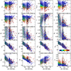 |
Fig. 22. Parameter values as a function of counts. The values are coloured according to the combined shape and concentration disturbance score, Dcomb. |
The fraction of clusters which have a high disturbance score Dcomb is relatively constant with the number of counts in the object. Using thresholds of 0, 25, 100, and 300 counts there are 27, 31, 27, and 25% of objects with scores greater than 0.5, respectively (see Fig. 23). 20% of clusters with more than 300 counts reach the higher disturbance threshold of Dcomb > 0.8, while 66% have a Dcomb < 0.2. Looking at clusters with more than 25 counts, there are 14% with Dcomb > 0.8 and 46% with Dcomb < 0.2. Fainter clusters have Dshape which lie more towards the centre of the range. This is likely because the shape parameters have large error bars when the number of counts is low, compared to the concentration, and therefore we know less about the cluster shape. In contrast, Dcomb is driven largely by concentration in the fainter objects.
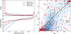 |
Fig. 23. Disturbance scores for the sample for clusters with greater than 25 and greater than 300 counts. Left: Histograms of the distributions of Dcomb (including concentration) and the purely 2D shape based Dshape. Right: Dcomb plotted against Dshape for the two count thresholds. |
As mentioned above, it matters which parameters were used to make the mixture model. In Fig. 23 are plotted the Dshape and Dcomb scores against each other for a sample of bright and fainter clusters. Although the scores are close for a substantial number of clusters, there are cases where they lie at opposite sides of the scale. The statistical uncertainty on concentration is typically much smaller than the other parameters, so it can drive the disturbance score when included. If Dshape is large, but Dcomb is small, this may indicate a cluster which has a disturbed shape but also a bright core. If Dcomb is large, but Dshape is small, this may indicate a symmetric cluster with a very flat surface brightness profile.
There is also some choice of how many clusters are initially fitted by the GMMs. We chose a threshold of 800 counts to ensure that statistical uncertainties on the input parameters were relatively small. We also reran the analysis using a threshold of 400 counts. The results were fairly similar, except the D scores were generally lower, with around 20% of objects classified as disturbed. If we increased the number of GGM components to three and fitted the combined parameters, we found that the third component has a low 4% amplitude compared to the others (64 and 32% for 800 counts) and lay at a more extreme position in the irregular cluster parameter space. Fitting the 400 count clusters yielded a similar result. If we added a fourth component, the modelling preferred this to have a low amplitude, with around 13% in the smallest two components. Therefore, the GGM model does not show strong evidence for more than two components.
Some examples of clusters with extreme low and high disturbance scores are shown in Fig. 24. In this brighter cluster regime, the parameter appears to be able to easily separate relaxed and disturbed clusters. The clusters include well known relaxed and disturbed objects.
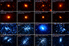 |
Fig. 24. Examples of eight relaxed and eight disturbed clusters. Clusters are randomly selected from the sample with more than 300 counts, where Dcomb = 0 (top panels) or Dcomb = 1 (bottom panels). The exposure corrected images in the 0.2–2.3 keV band have been smoothed with a Gaussian of σ = 8 arcsec or 64 arcsec in the case of 1eRASS J000842.4-570213. The bars show a fixed angular scale of 5 arcmin. |
We find a large fraction of relaxed objects. X-ray selection is better at finding clusters with dense central cores, likely associated with relaxed cool core clusters, while SZ selection finds a larger number of disturbed systems. As in some previous X-ray surveys, we found a large fraction of relaxed objects.
Rossetti et al. (2017) studied the morphology of clusters selected using the SZ effect by Planck, using Chandra and some XMM-Newton data. Based on the concentration in 40 and 400 kpc apertures, they find 29 ± 4% of their clusters are cool-core objects. They conducted the same measurement on the ROSAT all-sky X-ray selected MACS sample (Mann & Ebeling 2012), finding 59 ± 5% could be classified as cool-core.
Lovisari et al. (2017) studied the morphology of the Planck ESZ clusters using XMM-Newton. By visual inspection, they classify 32% of objects as relaxed, 39% disturbed and 29% were of an intermediate state. All of their clusters which are visually identified as relaxed have a concentration of more than 0.15 or c500 > −0.82 in our log units. Ignoring the statistical uncertainties on our values, this threshold would imply 80% of our eRASS1 objects are relaxed, similar to the fraction identified by our GMM.
Campitiello et al. (2022) studied the morphology of 188 clusters observed by XMM-Newton and selected using Planck. Using a combination of visual inspection and combining morphological parameters, they find 13% were robustly classified as relaxed, while 21% are disturbed.
Ghirardini et al. (2022) find that the X-ray selected eROSITA eFEDS cluster sample have a similar fraction of cool cores to SZ selected surveys. They constructed a relaxation score based on a combination of several morphological parameters, finding that concentration probes the inner part of the cluster but is not overall a good measure of relaxation. Around 70% of their clusters at the lowest redshifts are found to be relaxed, similar to what is found by us. However, this decreases rapidly to 35–50% at z > 0.2, becoming closer to the SZ-selected samples. This difference in relaxation over redshift could be evolution or selection effects.
9. Conclusions
We measured 29 morphological parameters for over 12 000 clusters found in the eROSITA survey by B24. The parameters we measured include concentration, central density, inner density slope, peak offset, power ratios, Gini coefficient, photon asymmetry, centroid shift, ellipticity, slosh, and multipole magnitudes. In our work, we have introduced new slosh and multipole magnitude forward modelled parameters. This paper provides a catalogue of the largest X-ray derived set of cluster morphological parameters to date.
Several of the measured quantities (e.g. power ratios, centroid shift, Gini coefficient, photon asymmetry) show values that correlate strongly with the number of counts, luminosity, or redshift. When we conducted simulations of clusters observed in the survey, we found similar relations. These correlations are are caused by biases due to noise or PSF, and therefore these parameters are unreliable for eROSITA clusters. We discussed the various biases that can be present in the parameters and provided the typical biases and uncertainties as a function of redshift and the number of counts.
Using both simulations and data, we observed that the concentration of clusters strongly affects whether they are detected in the eROSITA survey. At low redshifts (z ≲ 0.2), we preferentially detected more highly concentrated objects and did not detect low luminosity groups and clusters with flat surface brightness profiles. At high redshifts (z ≳ 0.4), we missed the most concentrated clusters. Alternative detection algorithms (e.g. wavelets) may find more flat surface brightness objects at low redshifts.
We made comparisons of our results for matched cluster subsamples for eRASS and other analyses. There is reasonable agreement in the concentration and density with matched Planck ESZ and SPT subsamples. The median values are close to those we obtained using eROSITA, although there may be mild offsets or differences in slopes between the analyses. These differences may be due to different analysis procedures, data quality, choice of cluster centre, and parametrisation or unresolved AGN in the datasets.
Comparing whole cluster samples, we found that eRASS1 clusters have higher concentrations than SPT, Planck ESZ, and eFEDS. The difference is around 0.3 dex in our log units, implying that the ratio of flux inside 0.1R500 to R500 is twice what is found in these other samples.
We constructed combined parameters based on a Gaussian mixture model for measuring the disturbance of clusters (Dshape and Dcomb), and we found that one-fourth of the objects are classified as disturbed. The high relaxation fraction is likely due to X-ray selection selecting highly concentrated clusters that are more likely to be relaxed.
Data availability
The table described in Appendix A is available at the CDS via anonymous ftp to cdsarc.cds.unistra.fr (130.79.128.5) or via https://cdsarc.cds.unistra.fr/viz-bin/cat/J/A+A/695/A160
Acknowledgments
This work is based on data from eROSITA, the soft X-ray instrument aboard SRG, a joint Russian-German science mission supported by the Russian Space Agency (Roskosmos), in the interests of the Russian Academy of Sciences represented by its Space Research Institute (IKI), and the Deutsches Zentrum für Luft- und Raumfahrt (DLR). The SRG spacecraft was built by Lavochkin Association (NPOL) and its subcontractors, and is operated by NPOL with support from the Max Planck Institute for Extraterrestrial Physics (MPE). The development and construction of the eROSITA X-ray instrument was led by MPE, with contributions from the Dr. Karl Remeis Observatory Bamberg & ECAP (FAU Erlangen-Nuernberg), the University of Hamburg Observatory, the Leibniz Institute for Astrophysics Potsdam (AIP), and the Institute for Astronomy and Astrophysics of the University of Tübingen, with the support of DLR and the Max Planck Society. The Argelander Institute for Astronomy of the University of Bonn and the Ludwig Maximilians Universität Munich also participated in the science preparation for eROSITA. The eROSITA data shown here were processed using the eSASS/NRTA software system developed by the German eROSITA consortium. E.B., V.G., A.L. and X.Z. acknowledge financial support from the European Research Council (ERC) Consolidator Grant under the European Union’s Horizon 2020 research and innovation program (grant agreement CoG DarkQuest No 101002585). Funded in part by the Deutsche Forschungsgemeinschaft (DFG, German Research Foundation) - 450861021.
References
- Abraham, R. G., van den Bergh, S., & Nair, P. 2003, ApJ, 588, 218 [NASA ADS] [CrossRef] [Google Scholar]
- Asplund, M., Grevesse, N., Sauval, A. J., & Scott, P. 2009, ARA&A, 47, 481 [NASA ADS] [CrossRef] [Google Scholar]
- Biffi, V., Borgani, S., Murante, G., et al. 2016, ApJ, 827, 112 [NASA ADS] [CrossRef] [Google Scholar]
- Bîrzan, L., Rafferty, D. A., McNamara, B. R., Wise, M. W., & Nulsen, P. E. J. 2004, ApJ, 607, 800 [Google Scholar]
- Bleem, L. E., Stalder, B., de Haan, T., et al. 2015, ApJS, 216, 27 [Google Scholar]
- Böhringer, H., & Werner, N. 2010, A&ARv, 18, 127 [Google Scholar]
- Böhringer, H., Schuecker, P., Pratt, G. W., et al. 2007, A&A, 469, 363 [NASA ADS] [CrossRef] [EDP Sciences] [Google Scholar]
- Böhringer, H., Pratt, G. W., Arnaud, M., et al. 2010, A&A, 514, A32 [NASA ADS] [CrossRef] [EDP Sciences] [Google Scholar]
- Brunner, H., Liu, T., Lamer, G., et al. 2022, A&A, 661, A1 [NASA ADS] [CrossRef] [EDP Sciences] [Google Scholar]
- Bulbul, E., Liu, A., Pasini, T., et al. 2022, A&A, 661, A10 [NASA ADS] [CrossRef] [EDP Sciences] [Google Scholar]
- Bulbul, E., Liu, A., Kluge, M., et al. 2024, A&A, 685, A106 [NASA ADS] [CrossRef] [EDP Sciences] [Google Scholar]
- Buote, D. A., & Tsai, J. C. 1995, ApJ, 452, 522 [Google Scholar]
- Campitiello, M. G., Ettori, S., Lovisari, L., et al. 2022, A&A, 665, A117 [NASA ADS] [CrossRef] [EDP Sciences] [Google Scholar]
- Cavaliere, A., & Fusco-Femiano, R. 1978, A&A, 70, 677 [NASA ADS] [Google Scholar]
- Clowe, D., Bradač, M., Gonzalez, A. H., et al. 2006, ApJ, 648, L109 [NASA ADS] [CrossRef] [Google Scholar]
- Comparat, J., Eckert, D., Finoguenov, A., et al. 2020, Open J. Astrophys., 3, 13 [Google Scholar]
- Eckert, D., Molendi, S., & Paltani, S. 2011, A&A, 526, A79 [NASA ADS] [CrossRef] [EDP Sciences] [Google Scholar]
- Edge, A. C., & Stewart, G. C. 1991, MNRAS, 252, 414 [NASA ADS] [CrossRef] [Google Scholar]
- Fabian, A. C. 2012, ARA&A, 50, 455 [Google Scholar]
- Foreman-Mackey, D., Hogg, D. W., Lang, D., & Goodman, J. 2013, PASP, 125, 306 [Google Scholar]
- Ghirardini, V., Bahar, Y. E., Bulbul, E., et al. 2022, A&A, 661, A12 [NASA ADS] [CrossRef] [EDP Sciences] [Google Scholar]
- Gianfagna, G., Rasia, E., Cui, W., et al. 2023, MNRAS, 518, 4238 [Google Scholar]
- Hudson, D. S., Mittal, R., Reiprich, T. H., et al. 2010, A&A, 513, A37 [NASA ADS] [CrossRef] [EDP Sciences] [Google Scholar]
- Johnson, R., Ponman, T. J., & Finoguenov, A. 2009, MNRAS, 395, 1287 [CrossRef] [Google Scholar]
- Käfer, F., Finoguenov, A., Eckert, D., et al. 2019, A&A, 628, A43 [Google Scholar]
- Käfer, F., Finoguenov, A., Eckert, D., et al. 2020, A&A, 634, A8 [Google Scholar]
- Kluge, M., Comparat, J., Liu, A., et al. 2024, A&A, 688, A210 [NASA ADS] [CrossRef] [EDP Sciences] [Google Scholar]
- Lau, E. T., Kravtsov, A. V., & Nagai, D. 2009, ApJ, 705, 1129 [NASA ADS] [CrossRef] [Google Scholar]
- Lau, E. T., Nagai, D., Kravtsov, A. V., Vikhlinin, A., & Zentner, A. R. 2012, ApJ, 755, 116 [NASA ADS] [CrossRef] [Google Scholar]
- Liu, A., Bulbul, E., Shin, T., et al. 2024, A&A, 688, A186 [NASA ADS] [CrossRef] [EDP Sciences] [Google Scholar]
- Lotz, J. M., Primack, J., & Madau, P. 2004, AJ, 128, 163 [NASA ADS] [CrossRef] [Google Scholar]
- Lovisari, L., Forman, W. R., Jones, C., et al. 2017, ApJ, 846, 51 [Google Scholar]
- Mann, A. W., & Ebeling, H. 2012, MNRAS, 420, 2120 [NASA ADS] [CrossRef] [Google Scholar]
- Markevitch, M., & Vikhlinin, A. 2007, Phys. Rep., 443, 1 [Google Scholar]
- McDonald, M., Bayliss, M., Benson, B. A., et al. 2012, Nature, 488, 349 [Google Scholar]
- McDonald, M., Benson, B. A., Vikhlinin, A., et al. 2013, ApJ, 774, 23 [NASA ADS] [CrossRef] [Google Scholar]
- McDonald, M., Allen, S. W., Bayliss, M., et al. 2017, ApJ, 843, 28 [Google Scholar]
- McNamara, B. R., & Nulsen, P. E. J. 2012, New J. Phys., 14, 055023 [NASA ADS] [CrossRef] [Google Scholar]
- Melchior, P., & Goulding, A. D. 2018, Astron. Comput., 25, 183 [Google Scholar]
- Merloni, A., Lamer, G., Liu, T., et al. 2024, A&A, 682, A34 [NASA ADS] [CrossRef] [EDP Sciences] [Google Scholar]
- Mittal, R., Hicks, A., Reiprich, T. H., & Jaritz, V. 2011, A&A, 532, A133 [NASA ADS] [CrossRef] [EDP Sciences] [Google Scholar]
- Mohr, J. J., Evrard, A. E., Fabricant, D. G., & Geller, M. J. 1995, ApJ, 447, 8 [NASA ADS] [CrossRef] [Google Scholar]
- Nurgaliev, D., McDonald, M., Benson, B. A., et al. 2013, ApJ, 779, 112 [NASA ADS] [CrossRef] [Google Scholar]
- O’Hara, T. B., Mohr, J. J., Bialek, J. J., & Evrard, A. E. 2006, ApJ, 639, 64 [Google Scholar]
- Panagoulia, E. K., Fabian, A. C., & Sanders, J. S. 2014, MNRAS, 438, 2341 [NASA ADS] [CrossRef] [Google Scholar]
- Poole, G. B., Fardal, M. A., Babul, A., et al. 2006, MNRAS, 373, 881 [Google Scholar]
- Pratt, G. W., Croston, J. H., Arnaud, M., & Böhringer, H. 2009, A&A, 498, 361 [NASA ADS] [CrossRef] [EDP Sciences] [Google Scholar]
- Predehl, P., Andritschke, R., Arefiev, V., et al. 2021, A&A, 647, A1 [EDP Sciences] [Google Scholar]
- Rafferty, D. A., McNamara, B. R., Nulsen, P. E. J., & Wise, M. W. 2006, ApJ, 652, 216 [NASA ADS] [CrossRef] [Google Scholar]
- Rasia, E., Meneghetti, M., & Ettori, S. 2013, Astron. Rev., 8, 40 [Google Scholar]
- Rossetti, M., Gastaldello, F., Eckert, D., et al. 2017, MNRAS, 468, 1917 [Google Scholar]
- Sanders, J. S., Fabian, A. C., Russell, H. R., & Walker, S. A. 2018, MNRAS, 474, 1065 [NASA ADS] [CrossRef] [Google Scholar]
- Santos, J. S., Rosati, P., Tozzi, P., et al. 2008, A&A, 483, 35 [NASA ADS] [CrossRef] [EDP Sciences] [Google Scholar]
- Seppi, R., Comparat, J., Bulbul, E., et al. 2022, A&A, 665, A78 [NASA ADS] [CrossRef] [EDP Sciences] [Google Scholar]
- Spergel, D. N., Bean, R., Doré, O., et al. 2007, ApJS, 170, 377 [NASA ADS] [CrossRef] [Google Scholar]
- Valdarnini, R., & Sarazin, C. L. 2021, MNRAS, 504, 5409 [NASA ADS] [CrossRef] [Google Scholar]
- Vikhlinin, A., Burenin, R., Forman, W. R., et al. 2007, in Heating versus Cooling in Galaxies and Clusters of Galaxies, eds. H. Böhringer, G. W. Pratt, A. Finoguenov, & P. Schuecker, 48 [Google Scholar]
- Vikhlinin, A., Burenin, R. A., Ebeling, H., et al. 2009, ApJ, 692, 1033 [Google Scholar]
- Voit, G. M. 2005, Rev. Mod. Phys., 77, 207 [Google Scholar]
- Wechsler, R. H., Bullock, J. S., Primack, J. R., Kravtsov, A. V., & Dekel, A. 2002, ApJ, 568, 52 [NASA ADS] [CrossRef] [Google Scholar]
- Weißmann, A., Böhringer, H., Šuhada, R., & Ameglio, S. 2013, A&A, 549, A19 [NASA ADS] [CrossRef] [EDP Sciences] [Google Scholar]
- Xu, W., Ramos-Ceja, M. E., Pacaud, F., Reiprich, T. H., & Erben, T. 2022, A&A, 658, A59 [NASA ADS] [CrossRef] [EDP Sciences] [Google Scholar]
- Yuan, Z. S., Han, J. L., & Wen, Z. L. 2022, MNRAS, 513, 3013 [NASA ADS] [CrossRef] [Google Scholar]
Appendix A: Catalogue description
Table A.1 describes the columns in the morphology catalogue, giving the column name and respective morphological parameter. Most of the parameters are dimensionless, except for the inner physical gas density.
Column names in morphology catalogue.
All Tables
All Figures
|
Fig. 1. Example models exhibiting the effect of the different shape parameters. Shown are an elliptical model (top left), a slosh model (top right), an M1 model (centre left), an M2 model (centre right), an M3 model (bottom left), and an M4 model (bottom right). For the models, we used an angle of θ = 30deg. The numeric values show the magnitude of the respective parameter. |
| In the text | |
|
Fig. 2. Corner plot of the median MBProj2D shape parameters for Chandra observations of clusters in the SPT cluster sample. The quantities are plotted against each other, while the rightmost panels show the probability density of the values. The Pearson correlation coefficient is shown in each panel. |
| In the text | |
|
Fig. 3. Example Chandra images from the SPT sample shown in Fig. 2. Top left: SPT-CLJ0014-4952 [ϵ = 0.85, H = 0.50, M1 = 0.36, M2 = 0.26, M3 = 0.06, M4 = 0.03]. Top right: SPT-CLJ0307-6225 [ϵ = 0.58, H = 0.75, M1 = 0.88, M2 = 0.37, M3 = 0.27, M4 = 0.28]. Bottom left: SPT-CLJ0304-4401 [ϵ = 0.75, H = 0.14, M1 = 0.64, M2 = 0.26, M3 = 0.33, M4 = 0.11]. Bottom right: SPT-CLJ2342-5411 [ϵ = 0.64, H = 0.08, M1 = 0.71, M2 = 0.38, M3 = 0.07, M4 = 0.07]. |
| In the text | |
|
Fig. 4. Morphological parameters against redshift. The parameters are plotted for the bright cluster subset (≥300 counts) with larger markers. The small markers show clusters with at least 25 counts, without plotting uncertainties. The colour scale shows the X-ray luminosity (log erg s−1 in the 0.2–2.3 keV band) inside an aperture of radius 800 kpc. The parameters are the central scaled gas density (ns, 0), central electron density (n50), concentration from 80–800 kpc (c80 − 800), concentration from 0.1R500 to R500 (c500), central density slope (α), slope at fixed radius (α50), ellipticity (ϵ), slosh (H), multiple magnitudes (M1 to M4), power ratios (P10 to P40), photon asymmetry (Aphot), centroid shift (w), Gini coefficient (G), and fit-peak offset (F). |
| In the text | |
|
Fig. 5. Parameters against number of counts in an 800 kpc aperture. These parameters are plotted for the bright cluster subset (≥300 counts) with larger markers. The small markers show clusters with at least 25 counts, without plotting uncertainties. The colour scale shows the cluster redshift. |
| In the text | |
|
Fig. 6. Parameters against X-ray luminosity. These parameters are plotted for the bright cluster subset (≥300 counts) with larger markers. The small markers show clusters with at least 25 counts, without plotting uncertainties. The X-ray luminosity is inside an 800 kpc radius aperture in the 0.2–2.3 keV band. The colour scale shows the cluster redshift. |
| In the text | |
|
Fig. 7. Corner plot of the median MBProj2D shape parameters for the bright cluster (≥300 count) subset. The quantities are plotted against each other, while the rightmost panels show the probability density distribution of each value. |
| In the text | |
|
Fig. 8. Correlation matrix between different parameters for the bright cluster subset. Values were measured for clusters with more than 300 counts to reduce the effect of the statistical errors. Log values were taken for the photon asymmetry, power ratios and centroid shift. We also show the correlation with log cluster luminosity (L500), log number of counts in R500 (cts500), and log redshift. |
| In the text | |
|
Fig. 9. Example cluster images and morphological parameters. The clusters chosen are those from the catalogue with between 920 and 1080 counts within 800 kpc radius and an uncertainty on the number of counts of less than 5%. The exposure-corrected images are in the 0.2–2.3 keV band with the same angular scale and have been smoothed by a Gaussian with σ = 8 arcsec. We show the cluster name, redshift, scaled central density (ns, 0), concentration (c80 − 800), ellipticity (ϵ), slosh (H), multipole magnitudes (M1 to M4), and peak-fit offset (F). |
| In the text | |
|
Fig. 10. Relationship between detection likelihood (ℒdet), extension likelihood (ℒext), counts, and morphological parameters. (Top panels) The median value of the concentration (c80 − 800; left), central scaled density (ns, 0; centre), and central slope (α; right), in grid points of ℒext and ℒdet. (Bottom panels) The median morphological parameter values for grid points of counts in an 800 kpc aperture and ℒdet or ℒext. |
| In the text | |
|
Fig. 11. Cumulative distribution of concentration for different subsamples of the eRASS1 catalogue. The cumulative distributions are shown as a function of exposure time (texp), number of counts in a 800 kpc aperture, detection likelihood (ℒdet), and extension likelihood (ℒext). The left panels show the distribution of c500, while the right panels show the distribution of c80 − 800. |
| In the text | |
|
Fig. 12. Selection function of clusters with different redshifts and luminosities as a function of concentration that were calculated from simulated observations of spherical clusters. The panels show the detected fraction of clusters at different redshift. For each redshift, we show the detection fraction as a function of concentration for different luminosities (erg s−1). The log concentration (c80 − 800) is computed from the input model profile and is binned into bins of 0.1 width. |
| In the text | |
|
Fig. 13. Median X-ray luminosity of clusters in bins of concentration. The left panel uses bins of c80 − 800, while the right panel shows c500. The uncertainties shown are calculated with bootstrap resampling. All eRASS1 clusters are included in this analysis. |
| In the text | |
|
Fig. 14. Fit-centred and peak-centred (∗) quantities as a function of the distance between the cluster peak and the best fit position for a cluster subsample with ℒext > 6 and ℒdet > 20. The median quantities in bins of F are shown with bootstrap resampling uncertainties. The shaded regions show the 1σ percentile width of the data points within each bin. |
| In the text | |
|
Fig. 15. Recovery of forward modelled parameters as a function of redshift and luminosity using maximum likelihood. The plots show the recovered parameter values as a function of redshift, for clusters with an input shape compared to an input spherical cluster. The error bar shows the average best fitting parameter and the uncertainty on the mean. The shaded region shows the 1σ range of the recovered best fitting parameters. The panels show shaped models with ϵ = 0.7, H = 0.3, M1 = 0.3, M2 = 0.3, M3 = 0.3, and M4 = 0.3, respectively, compared to the spherical models. |
| In the text | |
|
Fig. 16. Detection fraction as a function of redshift for different luminosities and shapes. |
| In the text | |
|
Fig. 17. Measured non-forward-modelled morphological parameters for simulated model clusters. Clusters are simulated with different luminosities and redshifts, after sampling from the mass function. The shaded region shows the 1σ range of recovered parameters of detected clusters simulated from spherical cluster models. The dotted and dashed lines show the median obtained parameters for non-spherical detected clusters with the parameters shown. |
| In the text | |
|
Fig. 18. Recovered parameter bias from simulated clusters as a function of the redshift and number of counts inside an 800 kpc radius circle. For the concentration, central density and cuspiness, shown is the difference between the recovered values and the input profile, after deprojecting the emissivity profile. For the shape parameters, ϵ, H and M1 to M4, we show the difference between the recovered and input values (0.7 for ϵ and 0.3 for the others), for simulations with non-spherical clusters. For the parameters w, Aphot and P10 to P40, we show the value for a spherical cluster. |
| In the text | |
|
Fig. 19. Recovered statistical uncertainty in measured parameters from simulated clusters. This is the standard deviation on the difference between the input and recovered values, as in Fig. 18. |
| In the text | |
|
Fig. 20. Comparison of concentration and scaled central density measurements for the same cluster samples between eRASS and other measurements. The two left columns compare c500 and its distributions, while the two right columns show ns, 0. Median values are plotted as vertical lines. The number of counts for the cluster in the eRASS1 or eRASS:4 data is indicated by the colour. Top row: 66 Planck ESZ and eRASS1-detected clusters, with XMM-Newton results from Lovisari et al. (2017) and using the eRASS1 peak values. Second row: 66 SPT and eRASS1-detected clusters, analysed using Chandra data and taking the peak values from eRASS1. Third row: 83 SPT-detected clusters, extracting the values from Chandra eRASS:4 data using similar analysis procedures. Bottom row: 69 clusters detected in both eFEDS and eRASS1. The eFEDS survey results are from Ghirardini et al. (2022), while the eRASS1 results are the best fit position values. For the top three rows, we compute the best fitting linear relation between the results, assuming a normal distribution around the relation. |
| In the text | |
|
Fig. 21. Cumulative distribution of parameters for SPT, Planck ESZ, and eFEDS clusters compared to eRASS1 for different detection thresholds. For eROSITA the solid lines show the values fixing the cluster position at the peak, while the dotted lines show the distribution for when the cluster position varies during the fit. Shown are the concentration (top left), cuspiness (top right), central scaled density (bottom left), and ellipticity (bottom right). Planck values are taken from Lovisari et al. (2017) and eFEDS values are obtained by Ghirardini et al. (2022). The eFEDS-like curves are for eRASS1 clusters with ℒdet > 5, ℒext > 6 and an exposure time between 1000 and 1400s, to match eFEDS. The median published log masses of the SPT, Planck and eFEDS samples are 14.7, 14.8, and 14.0, respectively. The eROSITA sample median log M⊙ masses are 14.4, 14.5, 14.6, and 14.8, for detection likelihood thresholds of 20, 40, 80, and 320, respectively. |
| In the text | |
|
Fig. 22. Parameter values as a function of counts. The values are coloured according to the combined shape and concentration disturbance score, Dcomb. |
| In the text | |
|
Fig. 23. Disturbance scores for the sample for clusters with greater than 25 and greater than 300 counts. Left: Histograms of the distributions of Dcomb (including concentration) and the purely 2D shape based Dshape. Right: Dcomb plotted against Dshape for the two count thresholds. |
| In the text | |
|
Fig. 24. Examples of eight relaxed and eight disturbed clusters. Clusters are randomly selected from the sample with more than 300 counts, where Dcomb = 0 (top panels) or Dcomb = 1 (bottom panels). The exposure corrected images in the 0.2–2.3 keV band have been smoothed with a Gaussian of σ = 8 arcsec or 64 arcsec in the case of 1eRASS J000842.4-570213. The bars show a fixed angular scale of 5 arcmin. |
| In the text | |
Current usage metrics show cumulative count of Article Views (full-text article views including HTML views, PDF and ePub downloads, according to the available data) and Abstracts Views on Vision4Press platform.
Data correspond to usage on the plateform after 2015. The current usage metrics is available 48-96 hours after online publication and is updated daily on week days.
Initial download of the metrics may take a while.