| Issue |
A&A
Volume 692, December 2024
|
|
|---|---|---|
| Article Number | A253 | |
| Number of page(s) | 15 | |
| Section | Cosmology (including clusters of galaxies) | |
| DOI | https://doi.org/10.1051/0004-6361/202451266 | |
| Published online | 17 December 2024 | |
Gas thermodynamics meets galaxy kinematics: Joint mass measurements for eROSITA galaxy clusters
1
School of Astronomy and Space Science, Nanjing University, Nanjing, Jiangsu 210023, China
2
Leibniz-Institute for Astrophysics, An der Sternwarte 16, 14482 Potsdam, Germany
3
Max Planck Institute for Extraterrestrial Physics, Giessenbachstrasse 1, 85748 Garching, Germany
4
Institute of Astronomy, National Central University, Taoyuan 32001, Taiwan
5
Institut für Physik und Astronomie, Universität Potsdam, Karl-Liebknecht-Straße 24/25, D-14476 Potsdam, Germany
6
INAF, Osservatorio di Astrofisica e Scienza dello Spazio, via Piero Gobetti 93/3, 40129 Bologna, Italy
⋆ Corresponding author; pli@nju.edu.cn
Received:
26
June
2024
Accepted:
13
November
2024
The mass of galaxy clusters is a critical quantity for probing cluster cosmology and testing theories of gravity, but its measurement could be biased, given that assumptions are inevitable in order to make use of any approach. In this paper, we employ and compare two mass proxies for galaxy clusters: thermodynamics of the intracluster medium and kinematics of member galaxies. We selected 22 galaxy clusters from the cluster catalog in the first SRG/eROSITA All-Sky Survey (eRASS1) that have sufficient optical and near-infrared observations. We generated multiband images in the energy range of (0.3, 7) keV for each cluster, and derived their temperature profiles, gas mass profiles, and hydrostatic mass profiles using a parametric approach that does not assume dark matter halo models. With spectroscopically confirmed member galaxies collected from multiple surveys, we numerically solved the spherical Jeans equation for their dynamical mass profiles. Our results quantify the correlation between dynamical mass and the line-of-sight velocity dispersion, log Mdyn = (1.296 ± 0.001)log(σlos2rproj/G)−(3.87 ± 0.23), with a root mean square (rms) scatter of 0.14 dex. We find that the two mass proxies lead to roughly the same total mass, with no observed systematic bias. As such, the σ8 tension is not specific to hydrostatic mass or weak lensing shears, but also appears with galaxy kinematics. Interestingly, the hydrostatic-to-dynamical mass ratios decrease slightly toward large radii, which could possibly be evidence for accreting galaxies in the outskirts. We also compared our hydrostatic masses with the latest weak lensing masses inferred with scaling relations. The comparison shows that the weak lensing mass is significantly higher than our hydrostatic mass by ∼110%. This might explain the significantly larger value of σ8 from the latest measurement using eRASS1 clusters than almost all previous estimates in the literature. Finally, we tested the radial acceleration relation established in disk galaxies. We confirm the missing baryon problem in the inner region of galaxy clusters using three independent mass proxies for the first time. As ongoing and planned surveys are providing deeper X-ray observations and more galaxy spectra for cluster members, we expect to extend the study to cluster outskirts in the near future.
Key words: galaxies: clusters: general / galaxies: clusters: intracluster medium / cosmology: observations / dark matter / X-rays: galaxies: clusters
© The Authors 2024
 Open Access article, published by EDP Sciences, under the terms of the Creative Commons Attribution License (https://creativecommons.org/licenses/by/4.0), which permits unrestricted use, distribution, and reproduction in any medium, provided the original work is properly cited.
This article is published in open access under the Subscribe to Open model. Subscribe to A&A to support open access publication.
1. Introduction
Studying the dynamics of galaxy clusters provides a useful way to constrain the nature of dark matter, as the cold dark matter model predicts that dark matter halos are in a universal profile (Navarro et al. 1996). It also helps test the universality of scaling relations that are mostly established in galaxies, such as the baryonic Tully-Fisher relation (McGaugh et al. 2000) and the radial acceleration relation (RAR, McGaugh et al. 2016; Lelli et al. 2017a; Li et al. 2018). Both scientific objectives require robust measurements of cluster mass profiles, which is nontrivial, as it often suffers from both technical and observational difficulties.
The commonly employed dynamical tracer to measure cluster mass profiles is the hot cluster gas via the assumption of hydrostatic equilibrium. Hot cluster gas emits X-ray photons, so they can be measured with X-ray observations. The first all-sky X-ray telescope ROSAT led to the construction of the Northern (NORAS) catalog of 495 clusters (Böhringer et al. 2000) and the Southern (REFLEX) catalog of 447 clusters (Böhringer et al. 2004). There are smaller-sky-coverage but deeper observations with the XMM-Newton telescope, such as the XMM-Newton Cluster Survey (XCS, Mehrtens et al. 2012) for 503 galaxy clusters and the XMM-Newton Cluster Archive Super Survey (X-CLASS, Koulouridis et al. 2021) for 1646 galaxy clusters. Deep follow-up programs are limited to tens to hundreds of galaxy clusters, such as the X-COP project (Eckert et al. 2017) and the CHEX-MATE project (Arnaud 2021). A big milestone has been reached by the latest all-sky survey telescope, eROSITA (Predehl et al. 2021), which has observed more than 1.2 million X-ray sources (Merloni et al. 2024), and identified more than 26 000 extended sources (Bulbul et al. 2024) in the first SRG/eROSITA All-Sky Survey (eRASS1). More than 12 000 extended sources have been identified by optical observations (Kluge et al. 2024), leading to the largest catalog of galaxy clusters with X-ray data available. The significant increase in the number of X-ray selected clusters suggests that studying cluster dynamics in a statistical way is becoming more and more promising.
Cluster galaxies have also been used as dynamical tracers, assuming they are in dynamical equilibrium. The total cluster mass can be estimated by building a scaling relation between the total velocity dispersion of cluster galaxies and the virial mass via simulations (Biviano et al. 2006; Munari et al. 2013; Saro et al. 2013). To derive dynamical mass profiles, one needs to solves the Jeans equation (e.g. Binney & Tremaine 2008). However, this approach suffers from two technical difficulties. First, dynamical mass is related to radial velocity dispersion and 3-D galaxy distribution through the spherical Jeans equation (Binney & Tremaine 2008), but observationally only projected spatial distributions and line-of-sight velocity dispersion of member galaxies are measurable. Second, there is a serious degeneracy between dynamical mass and velocity anisotropy. Degeneracy is a general problem in astronomy that can lead to unrealistic estimations of parameters and even result in absurd conclusions (e.g. see Li et al. 2021). Mamon et al. (2013), Biviano et al. (2013) proposed to tackle these problems by parameterizing mass profiles, tracer distribution functions, and velocity anisotropy profiles using 3D functions. These functions are determined by matching their projected forms with observed phase-space information. Li et al. (2023a) also used parameterized profiles but with more flexible functions, and addressed the mass-velocity anisotropy degeneracy by introducing additional constraints that involve two virial shape parameters; namely, the fourth order of velocity dispersion (Merrifield & Kent 1990). As a result, the dynamical mass profiles can be well derived (see Appendix B in Li et al. 2023a).
Both approaches assume that galaxy clusters are relaxed, which cannot be independently, robustly verified. An interesting fact is that the two approaches assume different relaxations, one on hot intracluster gas via thermodynamics, and the other on member galaxies through kinematic motions. It is therefore interesting to compare these two mass estimators in a statistical sense. This is particularly interesting because of the σ8 tension (Planck Collaboration XXIX 2014), since the cluster mass measurements using hot gas are thought to be biased lower due to nonthermal flows (e.g. Lau et al. 2009; Vazza et al. 2009; Battaglia et al. 2012; Nelson et al. 2014; Shi et al. 2015; Biffi et al. 2016) and thereby lead to lower matter fluctuation compared with that from cosmic microwave background fluctuations (Planck Collaboration XIII 2016).
In this paper, we select a subsample of galaxy clusters from the cluster catalog in the first all-sky survey of eROSITA (Bulbul et al. 2024) based on their optical properties (Kluge et al. 2024). We measure their cluster mass profiles using both hot intracluster gas and cluster galaxies as dynamical tracers and make a systematic comparison between these two mass proxies. The paper is organized as follows: Section 2 describes our sample selection criteria; Sects. 3 and 4 present the results of X-ray analysis and kinematics analysis, respectively; Sect. 5 compares the mass profiles measured with different estimators; Sect. 6 shows a test for the universality of the RAR; and Sect. 7 discusses the results and concludes the paper.
2. Sample selection
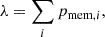
In this work, we have selected galaxy clusters from the eRASS1 cluster catalog (Bulbul et al. 2024). The main selection criterion is that there are both X-ray data and a sufficient number of member galaxies with spectroscopic redshift information, so that both gas thermodynamics and galaxy kinematics are applicable to measure cluster mass profiles. Since eROSITA clusters are X-ray selected, the major limitation comes from the effective number of member galaxies, defined as the summation of membership probability of cluster galaxies,
where pmem, i denotes the membership probability of individual galaxies. This definition differs from the optical richness (Kluge et al. 2024) by a scaling factor, which compensates for masked area and limited observational depth. Since we study galaxy kinematics, completeness is less important (see Appendix A in Li et al. 2023a). As such, we do not need the true richness, which requires a complete sample. However, we distinguish between photometric and spectroscopic richness. Photometric richness is simply the effective number of galaxies that are brighter than a threshold magnitude, while spectroscopic richness refers to spectroscopically confirmed galaxies. Photometric richness is generally larger than spectroscopic richness, given that spectra are more expensive to obtain. We determined the galaxy number density based on photometric richness, since it is more complete, while we measured velocity dispersion using spectroscopic redshifts, given that they are more accurate. To ensure robustness, we used 25 effective galaxies to calculate the line-of-sight velocity dispersion for each radial bin, and required at least two bins for galaxy number density and one bin for velocity dispersion. Therefore, our major limitation is the availability of galaxy spectra, which significantly reduces the size of our sample.
In order to assume spherical symmetry, we selected only clusters that can be approximately modeled with a single center; namely, requiring the offset between the X-ray center and optical center smaller than 60 kpc, following Tian et al. (2021). X-ray centers were determined by fitting X-ray images using the public code MBProj2D by Sanders et al. (2018) and the best-fit X-ray centers are given in Bulbul et al. (2024). Optical centers correspond to the positions with the minimum gravitational potential due to cluster galaxies, or equivalently the positions with the highest luminosity weighted galaxy number density (Rykoff et al. 2014, 2016; Kluge et al. 2024). We identified the brightest cluster galaxies (BCGs) based on their z-band magnitude, and selected clusters with BCGs in the optical centers. Given these criteria, although X-ray and optical data were analyzed using their own centers, we do not distinguish the centers of the derived mass profiles throughout the paper.
We excluded clusters that are undergoing merging, such as the cluster J090911.9+105835, as their velocity distribution histograms of member galaxies present clear double peaks. In summary, we selected clusters from the eRASS1 cluster catalog by Bulbul et al. (2024) based on three criteria: (1) there are at least 25 effective spectroscopic galaxies and 50 effective photometric galaxies; (2) their BCG position, X-ray, and optical centers are roughly consistent; (3) clusters are not merging. Eventually, our sample includes 22 clusters. Their properties and other names in various published catalogs are given in Tables 1 and A.1, respectively. The sample covers a large range in redshift, up to ∼0.77. The data quality also varies significantly, from around 50 photons to more than 2000 photons in the band of (0.2, 2.3) keV. Though the current sample is small compared to the large cluster sample in the eRASS1 catalog, we expect to significantly expand the sample in a few years with the help of dedicated observations by the black hole mapper of SDSS-V (Almeida et al. 2023) and the galaxy cluster survey of 4MOST (Finoguenov et al. 2019; de Jong et al. 2019). The X-ray data quality will also be five times better once the eRASS:5 is made available.
Properties of the 22 selected clusters.
3. Gas thermodynamics from X-ray observations
3.1. Generating X-ray images
The X-ray data for the selected 22 clusters are from the first all-sky survey by eROSITA from December 2019 to June 2020. There is one cluster (1eRASS J090131.5+030055) appearing in the eFEDS cluster catalog (Liu et al. 2022), so we combined the X-ray data from both data releases to increase the exposure time. We processed the data with the eROSITA Science Analysis Software System (eSASS1, Brunner et al. 2022). From the calibrated photon event lists, we constructed images and exposure maps in seven energy bands: [0.3–0.6], [0.6–1.0], [1.0–1.6], [1.6–2.2], [2.2–3.5], [3.5–5.0], and [5.0–7.0] keV. X-ray photons were collected from all seven telescope modules (TMs) for hard bands. For the two soft bands with energy lower than 1 keV, we excluded photons from TM 5 and TM 7 due to light leak (Predehl et al. 2021). We set a fixed image size as 6 Mpc × 6 Mpc, which is sufficiently large to robustly estimate background levels.
Figure 1 shows an example image for 1eRASS J004207.0-283154 in the energy range [0.3, 7] keV. It shows the exposure-map-corrected counts. We masked the point sources that are identified in Merloni et al. (2024) and galaxy clusters in Bulbul et al. (2024). The radii of the masked point sources were determined by the point spread function (PSF) scaled by their count rates (ML_RATE_1 in Merloni et al. 2024), so that brighter sources were masked with a larger area, while the radii of masked background clusters were chosen as their half R500. We also masked the four corners, so that only the colored region was used for the following analysis2.
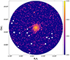 |
Fig. 1. X-ray image of 1eRASS J004207.0-283154 with exposure map corrected in the energy range of (0.3–7.0) keV, smoothed with Gaussian filters. Small white circles show the masked regions that were selected using the X-ray source catalog (Merloni et al. 2024) and the cluster catalog (Bulbul et al. 2024). The color bar labels the exposure-map-corrected X-ray photon counts. |
3.2. Fitting X-ray images
We fit the X-ray images with the public Multi-Band Projector 2D code (MBProj2D, Sanders et al. 2018; Bulbul et al. 2024). MBProj2D fits multiple band images and their associated backgrounds simultaneously using a Markov chain Monte Carlo approach. We have assumed the same PSF for all the seven TMs. Both the ancillary response file and the redistribution matrix file are implemented in the code. The Galactic hydrogen column density is also properly taken into account.
By fitting multiband images, we measured temperature profiles, electron number density profiles, and thereby gas mass profiles. Usually, the temperature profiles of galaxy clusters are measured from X-ray spectra. However, this requires a long exposure time, which is hardly achievable for many eROSITA clusters. From multiband images, we can derive roughly the same temperature profiles as those from spectra (Liu et al. 2023). We parameterized the temperature profile using the McDonald model (McDonald et al. 2014),
![$$ \begin{aligned} T(r) = T_0\frac{(r/r_{\rm cool})^{a_{\rm cool}}+T_{\rm min}/T_0}{(r/r_{\rm cool})^{a_{\rm cool}}+1}\cdot \frac{(r/r_t)^{-a}}{[1+(r/r_t)^b]^{c/b}}, \end{aligned} $$](/articles/aa/full_html/2024/12/aa51266-24/aa51266-24-eq68.gif)
where cool cores within rcool are accommodated with the temperature of Tmin. We fixed the parameters a = 0 and b = 2. Therefore, the temperature profile has six free parameters. We imposed the following flat priors: 0 < acool < 2, 0 < c < 2, −2.3 < ln(T0/keV) < 3, 0.1 < Tmin/T0 < 1.5, 0.1 < rcool < 2000 kpc, and 10 < rt < 5000 kpc. Some of the priors were imposed following Ghirardini et al. (2019). We slightly narrowed down some ranges considering the actual fits.
We modeled the electron number density profile, ne, using the single-β component Vikhlinin model (Vikhlinin et al. 2006),
where np is the proton number density and assumed to be np = ne/1.21. We fixed γ = 3 and imposed flat priors on the six free parameters: 0 < α < 5, 0 < β < 5, 0 < ϵ < 5, −8 < ln(n0/cm−3) < 2, 100 < rs < 5000 kpc, and 1 < rc < 500 kpc. Those ranges are much wider than the typical variations in the properties of galaxy clusters.
We assumed a constant metallicity profile with 0.3 solar abundance using the solar value from Lodders (2003), and spatially constant background emissions in different energy bands. In order to minimize the number of free parameters, we fixed the centers of galaxy clusters using the values from Bulbul et al. (2024). As such, there are 19 fitting parameters in total: 6 in the density profile, 6 in the temperature profile, and 7 for the background levels in the seven energy bands. We used the emcee hammer (Foreman-Mackey et al. 2013) to draw their posterior distributions. We set up 190 random walkers and ran 5000 iterations with the first 1000 steps being the burnt-in phase. These are more than sufficient to achieve convergence.
We used non-hydro modeling for clusters in MBProj2D, which incorporates the aforementioned density, temperature, and metallicity profiles, but does not assume any models for dark matter halos. One major improvement of MBProj2D over its previous version is that it fits 2D images rather than azimuthally averaged surface brightness profiles. Therefore, we can check the fit quality by examining the corresponding surface brightness profile. As an example, Fig. 2 shows the surface brightness profiles of 1eRASS J004207.0-283154 in six energy bands. We do not show the profile in the hardest band (5–7 keV) as it is dominated by background emissions and thereby remains flat. The binned surface brightness profiles in all the energy bands are well described by the total model, which is the summation of the background level and the cluster model. This verifies the image fitting.
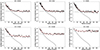 |
Fig. 2. Surface brightness profiles of 1eRASS J004207.0-283154 in six different energy bands. The azimuthally averaged surface brightness in each band is compared with the total model (red lines), which is the summation of the constant background (dashed black lines) and the cluster model (solid black lines). Cluster models are truncated at 2 Mpc. |
We directly derived electron number density profiles and temperature profiles from their Markov chains by calculating their median values, rather than using the functional forms and their best-fit parameters. As such, the median profiles may not be smooth curves (for example, see Fig. 3). The two approaches usually lead to slightly different results, but generally consistent within their errors. We list the best-fit parameters in Table 2 so that one can easily reproduce these profiles. The top right panel of Fig. 3 shows that the errors on the temperature profile are quite large. This is not because we only fit images or due to an insufficient number of photons, given that Liu et al. (2023) found similarly large errors using the X-ray spectra for a luminous cluster. In fact, the temperature of ICM is generally poorly constrained.
 |
Fig. 3. Electron number density (top left), temperature (top right), cumulative gas mass (bottom left), and hydrostatic mass (bottom right) profiles of 1eRASS J004207.0-283154. Solid lines and shadow regions are the median values and the corresponding 68% confidence limits, respectively. Both the mean values and the uncertainties were directly extracted from their Markov chains. Notice that the profiles can also be derived using the median values in the posterior distributions of the fitting parameters in Table 2. This approach could lead to slightly different profiles from those extracted from Markov chains, but consistent within 1σ. The latter generally results in non-smooth curves. The complete figure set for all clusters is available at Zenodo. The data for these profiles are available at Github (https://pengfeili0606.github.io/data). |
Best-fit parameters for the temperature profile (first six parameters) and the electron number density profile (last six parameters).
3.3. Gas mass and hydrostatic mass
The cumulative gas mass profiles can be calculated from the electron number density by

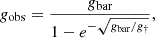
where mp is the mass of protons, A ≃ 1.4 is the mean nuclear mass number, and Z ≃ 1.2 is the charge number of the intracluster medium (ICM) with 0.3 solar abundance (Anders & Grevesse 1989). To derive the total mass profile using the ICM as the dynamical tracer, one assumes that the ICM is in hydrostatic equilibrium; that is, that the pressure gradient counteracts the radial gravity. One relates the pressure profile of the ICM to its temperature and electron number density using the ideal gas law, p(r) = ne(r)kBT(r), where kB is the Boltzmann constant. As such, the hydrostatic mass is given by
where the mean molecular weight is μ ≃ 0.6 for the assumed 0.3 solar abundance.
The bottom panels of Fig. 3 show example profiles of cumulative gas mass and hydrostatic mass profiles for 1eRASS J004207.0-283154. Both were calculated from the derived Markov chains of the fitting parameters without assuming dark matter halo models, so our results are independent of halo models. The hydrostatic mass profile presents larger uncertainties than the gas mass profile. This is mainly driven by the large uncertainties on the temperature profiles. We derived the mass profiles up to 2 Mpc for all clusters, as hydrostatic equilibrium is generally broken at larger radii.
4. Cluster dynamics from galaxy kinematics
4.1. Cluster galaxies
In this paper, we also employed cluster galaxies as dynamical tracers to derive the total mass profiles for the selected eROSITA clusters. We used the member galaxies compiled by Kluge et al. (2024). Kluge et al. (2024) identified cluster galaxies using both the optical and near-infrared photometry from the ninth and tenth data releases of the DESI Legacy Imaging Surveys (Dey et al. 2019). Using the red-sequence matched-filter probabilistic percolation cluster finder (redMaPPer, Rykoff et al. 2014, 2016), the membership probabilities for individual galaxies were determined, which are dependent on color distance from red-sequence models (e.g. Oguri 2014), spatial distributions, galaxy luminosity, and background galaxy number density. The photometric redshift of each member galaxy was also measured. Considering its large uncertainty, we only used galaxies with spectroscopic redshift to calculate the velocity dispersion. Kluge et al. (2024) collected more than 4.8 million spectroscopic galaxy redshifts from the literature. The major contributors are Zou et al. (2019), Colless et al. (2001), Coil et al. (2011), Cool et al. (2013), Alam et al. (2015), and Ahumada et al. (2020). Those spectra were obtained with multiple surveys including 2dFGR (Colless et al. 2001), 6dFGR (Jones et al. 2004, 2009), 2SLAQ (Cannon et al. 2006), DEEP2 (Davis et al. 2003; Newman et al. 2013), SDSS DR14 (Abolfathi et al. 2018), and zCOSMOS (Lilly et al. 2007).
The cluster galaxies from Kluge et al. (2024) are red-sequence galaxies, which are known to be more concentrated toward the cluster center (Nishizawa et al. 2018), but also have larger velocity dispersion than blue galaxies (e.g. see Binggeli et al. 1987). Therefore, using red-sequence galaxies alone does not necessarily introduce bias, as the enclosed total mass is correlated with σ2r (Binney & Tremaine 2008). Instead, red-sequence galaxies are older than blue galaxies, so that they are presumably more likely relaxed. As such, employing only red-sequence galaxies as dynamical tracers is technically safer, though ideally the two populations should lead to roughly the same results if both are relaxed.
As an example, Fig. 4 plots the phase-space distribution of the member galaxies for 1eRASS J004207.0-283154. It is a general phenomenon that a significant fraction of member galaxies do not have a measured spectroscopic redshift, and we only used spectroscopically confirmed galaxies to calculate the line-of-sight velocity dispersion profile. As such, there are often more bins in the galaxy surface number density profile than that for velocity dispersion (see Fig. 5). We stress that when calculating velocity dispersion, the cosmological effect has to be taken into account (Harrison 1974; Danese et al. 1980). This is because the observed redshift, zobs, is the product of two contributions,

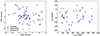 |
Fig. 4. Example phase-space distributions of cluster galaxies. Left panel: Spatial distribution of the member galaxies of 1eRASS J004207.0-283154 on the projected sky. Red upward triangles and blue downward triangles represent receding and approaching galaxies, respectively. Black points are galaxies without spectroscopic redshift. Right panel: Line-of-sight velocities of the member galaxies with respect to the BCG against the projected radii, rproj. Galaxies with only photometric redshift are excluded in this plot. Cluster 004207.0-283154 presents a slightly asymmetric velocity distribution of its member galaxies. This does not affect the binned velocity dispersion, as galaxies within each bin were fit using the generalized Gaussian function, which allows a variable mean velocity (see Sect. 4.2). |
where zcosmos is the cosmological redshift, or approximately the redshift of the host cluster, and zpeculiar is the redshift due to peculiar motions of cluster galaxies. As such, the peculiar redshift difference between two member galaxies at roughly the same radii is given by (Harrison 1974; Kluge et al. 2024)

To be precise, we used the Doppler equation to calculate the relative velocity,
![$$ \begin{aligned} \Delta v_{\rm los} = c[(\Delta z_{\rm peculiar}+1)^2 - 1 ] / [ (\Delta z_{\rm peculiar}+1)^2 + 1 ], \end{aligned} $$](/articles/aa/full_html/2024/12/aa51266-24/aa51266-24-eq74.gif)
instead of Δvlos = cΔzpeculiar, though they are quite close given that Δzpeculiar ≪ 1 in general.
We notice that the velocity distribution of member galaxies with respect to the BCG could be slightly asymmetric. This does not affect the binned velocity dispersion, as we fit the galaxy velocity distribution within each bin using Binulator developed by Collins et al. (2021). The Binulator fits a generalized Gaussian function, allowing a varying mean value. With Binulator, velocity dispersion can be robustly determined even if the sample size is as low as 25 effective galaxies in each bin. As is shown in Fig. 5, some clusters have only one binned line-of-sight velocity dispersion, so that their fit velocity profiles and thereby dynamical mass profiles are unreliable. To avoid overextrapolations, we did not use the whole mass profiles, but only the discrete values at the radii where the actual binned velocity dispersion is available.
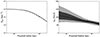 |
Fig. 5. Example fits to the binned cluster galaxies. Left: Galaxy surface number density profile. Points with errors are for the binned photometrically selected galaxies. The solid line is the fit profile with three projected Plummer spheres (Plummer 1911). Right: Line-of-sight velocity dispersion profile. The single point with errors is the binned velocity dispersion using spectroscopically selected galaxies, while the solid line is the expected profile based on the fit mass profile parameterized by the coreNFWtides model (Read et al. 2016). The dark and light shadow regions present 1σ and 2σ limits, respectively. In both profiles, membership probabilities of galaxies are considered when binning. To be consistent with previous figures, the example shown is from 1eRASS J004207.0-283154. |
4.2. Jeans modeling
Employing cluster galaxies as dynamical tracers makes use of Jeans modeling. This approach has been developed and thoroughly described in Li et al. (2023a). Readers interested in more details are recommended to read this paper. We only mention some main points here. The equation that relates velocity dispersion to dynamical mass is the Boltzmann equation (Binney & Tremaine 2008). When assuming spherical symmetry, it becomes the Jeans equation given by

where the number density of member galaxies, ν(r), and the radial velocity dispersion, σr, can be derived by fitting their projected profiles to observations; the total mass profile, M(r), is the target quantity. The velocity anisotropy parameter, β = 1 − σt2/σr2, relates the radial velocity dispersion, σr, and tangential velocity dispersion, σt. To determine its profile, one solves the projected, integrated Jeans equation (van der Marel 1994; Binney & Mamon 1982),
where the projected distribution of galaxies (Σgal) and line-of-sight velocity dispersion (σlos) are directly observable (see Fig. 5).
To solve Eqs. (9) and (10), we used the GravSphere code (Read & Steger 2017), which has been tested with simulations for many different systems (Read & Steger 2017; Read et al. 2018, 2021; Collins et al. 2021; Genina et al. 2020; De Leo et al. 2024). GravSphere parameterizes the galaxy number density, ν(r), velocity anisotropy, β(r), and dynamical mass profile, M(r), with successive functions. The galaxy number density is modeled with three Plummer spheres (Plummer 1911). It can be determined by fitting its projected function,
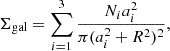
to the binned galaxy surface number density (see Fig. 5). In Eq. (11), Ni are dimensionless and chosen to satisfy ∫ν(r)d3r = 1, and ai are scale radii that quantify how concentrated galaxies’ distributions are. They are generally in the range of 10−4 < Ni < 100 and 50 kpc < ai< 2000 kpc.
The velocity anisotropy profile, β(r), is parameterized by a function with four parameters,
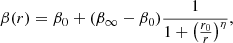
where β0 and β∞ quantify the anisotropies at r = 0 and r = ∞, respectively; r0 and η characterize the radial shape. The cumulative dynamical mass profile, M(< r), is described by six parameters using the cored-NFW-tides model (cNFWt, Read et al. 2018); that is, McNFWt(< r) =
![$$ \begin{aligned} {\left\{ \begin{array}{ll} M_{\rm cNFW}(<r) = M_{\rm NFW}(<r)f^n&\text{ if}\ r\le r_t,\\ M_{\rm cNFW}( < r_t) + 4\pi \rho _{\rm cNFW}(r_t)\frac{r_t^3}{3-\delta }\Big [\Big (\frac{r}{r_t}\Big )^{3-\delta }-1\Big ]&\text{ if}\ r>r_t,\\ \end{array}\right.} \end{aligned} $$](/articles/aa/full_html/2024/12/aa51266-24/aa51266-24-eq80.gif)
where MNFW and McNFW are the cumulative mass profiles of the Navarro-Frenk-White (NFW, Navarro et al. 1996) and cored NFW (cNFW, Read et al. 2016) models, respectively;  and n generate cored density profiles with rc being the core scale radius;
 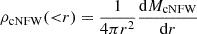 ; rt is the transition radius; and δ is the outer density slope. As such, the cNFWt profile is a flexible function accommodating variable inner and outer slopes.
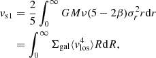
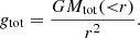
A major advantage of the approach developed in Li et al. (2023a) is the usage of two virial shape parameters (Merrifield & Kent 1990),
where ⟨⟩ denotes the mean. The two virial shape parameters introduce additional constraints on velocity anisotropy and dynamical mass, so that their degeneracy (see Eq. (9)) is ameliorated.
The parameterized functions for M(r), β(r) and ν(r) are quite flexible. This is intended to maximize the allowed solution space, so that the results are mainly driven by the data rather than by the chosen models. GravSphere makes use of the Markov chain Monte Carlo method with the emcee hammer by Foreman-Mackey et al. (2013) to map the posterior distributions of the parameter space in Eqs. (12) and (13). Following Li et al. (2023a), we set the below hard boundaries for the parameters in the cNFW model: 13 < log(M200/M⊙) < 20, 0.1 < c200 < 100, 10 kpc < rc< 3000 kpc, −0.5 < n < 2.0, 10 kpc < rt< 5000 kpc, and 0 < δ < 3. For β(r), we required that 1 < n < 3 and 0.5Rhalf < r0 < 2Rhalf, where Rhalf is the half-mass radius. The anisotropies in the center and infinity were constrained in a symmetrized form to avoid infinite values: 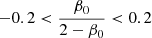 and
and 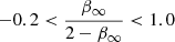 . There are ten fitting parameters in total. We imposed flat priors within the aforementioned boundaries. We used 150 walkers and ran 104 steps to guarantee convergence.
4.3. The effect of interlopers
A major concern using member galaxies as dynamical tracers is interlopers, which could be mistakenly counted as members. They could affect the galaxy number density and velocity dispersion measurements, and thereby the final mass profiles. We minimized this effect in two ways. First, we used membership probabilities to weigh the effective number of each candidate. The membership probability of each member candidate was estimated with eROMapper (Kluge et al. 2024), which is built upon the red-sequence matched-filter probabilistic percolation cluster-finding algorithm (Rykoff et al. 2014, 2016). Under this scheme, a candidate with a membership probability smaller than 100% will be assigned an effective number smaller than one. Unless the membership probability of an interloper is seriously overestimated, its contributions to galaxy number density and velocity dispersion would be negligible. Second, the line-of-sight velocity dispersion within each radial bin was not directly calculated based on the velocities of all members, but derived by fitting a generalized Gaussian function to the effective number histogram of line-of-sight velocities using Binulator (Collins et al. 2021). As such, a single miscounted interloper plays little role in the measurement of velocity dispersion. With these two measures combined, even a group of miscounted galaxies do not have significant impact on our results, as they should have small membership probabilities. As such, we do not worry about interlopers in our dynamical approach.
4.4. Spatially resolved mass-velocity dispersion relation
By running Gravsphere, we derived the dynamical mass profiles for the 22 eROSITA clusters. Dynamical mass is expected to be correlated with velocity dispersion (Binney & Tremaine 2008). However, the specific coefficients are unknown. By numerically solving Jeans equation with Gravsphere, we were able to determine the relation in an empirical way. To increase the statistics, we also included the 10 clusters from Li et al. (2023a), given that their dynamical masses were derived in the same way. We did not distinguish clusters at different redshifts, as we derived the scaling relation directly from the Jeans equation, which does not evolve with time.
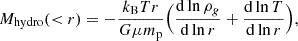
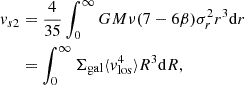
Figure 6 plots the dynamical mass against the product of σlos2rproj/G for the 22 eROSITA clusters and 10 HIFLUGCS clusters. Each point represents a single value at a specific radius rather than a cluster. The 32 clusters present a tight linear correlation in logarithmic space, which can be nicely fit by

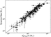 |
Fig. 6. Enclosed dynamical mass against the product σlos2rproj/G for 22 eROSITA clusters and 10 HIFLUGCS clusters from Li et al. (2023a). Note that velocity dispersion is measured at rather than within a specific radius, i.e., σlos = σlos(R = rproj)≠σlos(R < rproj), while the dynamical mass is cumulative, Mdyn = Mdyn(r < rproj), where R and r are 2D and 3D radii, respectively; rproj is the projected radius. The correlation can be described by a power law (the solid line): log Mdyn = (1.296 ± 0.001)log(σlos2rproj/G)−(3.87 ± 0.23). The total scatter is 0.14 dex (∼32%). To clarify, points with errors are the binned results at different radii, so a cluster could have more than one point. |
where σlos(R) is the line-of-sight velocity dispersion at R = rproj rather than R < rproj, while Mdyn(< R) is the cumulative mass within the 3D radius r = rproj. The root mean square (rms) scatter around the fit relation is 0.14 dex. This is partially contributed to by the deviation from the best-fit mass profile (e.g., see the right panel of Fig. 5. The best-fit line does not exactly cross the point), especially when there is more than one binned velocity dispersion. The actual scatter of the correlation could therefore be even smaller. Besides, clusters could have very different velocity anisotropy profiles, which are also radially dependent. This diversity is another source for the total scatter.
We note that the slope of the fit line is not one, as one might expect from the commonly used equation Mdyn = cσlos2rproj/G (Binney & Tremaine 2008; Kluge et al. 2024), where c is the proportional coefficient. The coefficient is not a constant, therefore, but depends on mass or radius. In other words, the correlation is approximately a power law, rather than linear. This is evident from Eq. (9), which considers not only velocity dispersion, but also its radial derivative. The derivative term contributes additional dependency on velocity dispersion that steepens the slope in log space. In addition, velocity anisotropy varies radially as well, so it could also affect the slope.
Equation (16) can be thought of as a simplified version of the complicated Jeans equation. It is a spatially resolved relation, differing from the σlos − M200 relation. The latter is frequently studied in the literature (e.g. Munari et al. 2013), and evolves with redshift, since the definition of M200 depends on the critical density of the Universe. The data points that are used to determine Eq. (16) range from 68 kpc to 3820 kpc in radius, and from 533 km/s to 1336 km/s in velocity dispersion. It can be used to quickly determine the cumulative dynamical mass of a galaxy cluster at different radii with an accuracy of ∼32% (0.14 dex). By astronomical standards, this is sufficiently accurate in many situations. Despite the above relation not relying on the assumption of the dynamical states of considered systems, it is indeed assumed that cluster galaxies are relaxed and stay in dynamical equilibrium with the whole cluster when used for mass estimations.
5. Comparison of different mass proxies
Comparing different mass estimators is useful for a consistency check, which is of interest given that every proxy relies on some assumption, such as the hydrostatic equilibrium for gas thermodynamics and dynamical relaxation for galaxy kinematics. Of particular interest is to investigate the so-called hydrostatic bias, which is on the one hand motivated by the existence of nonthermal flow in the ICM (Lau et al. 2009; Vazza et al. 2009; Battaglia et al. 2012; Nelson et al. 2014; Shi et al. 2015; Biffi et al. 2016; Liu et al. 2016, 2018), and on the other hand indicated by the σ8 tension, as cluster mass from Sunyaev-Zeldovich effect used to be calibrated with hydrostatic mass (Planck Collaboration XXIV 2016). Multiple approaches have been employed to quantify hydrostatic bias, such as assuming a constant cosmic baryonic fraction at different cluster radii (Eckert et al. 2019), comparison with weak lensing mass (Donahue et al. 2014; von der Linden et al. 2014; Sereno et al. 2015; Hoekstra et al. 2015; Penna-Lima et al. 2017; Sereno et al. 2017). No agreement has been reached in terms of the degree of the bias, and none of these studies found the level required for resolving the σ8 tension. Foëx et al. (2017) compared the dynamical masses measured with the Jeans, caustic, and virial-theorem approaches to hydrostatic masses, and found that they are generally 20%-50% higher. Li et al. (2023a) developed a more sophisticated Jeans approach, which showed a 50% higher dynamical mass on average. Both studies have only ten clusters, so the results remain inconclusive.
In Fig. 7, the left panel plots the dynamical mass against hydrostatic mass for the 22 eROSITA clusters. We also collected the ten HIFLUGCS clusters from Li et al. (2023a). Since the hydrostatic masses of these two samples were measured with different approaches, we distinguish them with different colors. It should be noted that we are not comparing the total mass, but the enclosed mass at different radii. The former is often compared because of cosmological interests. The practical reason is that we do not have a sufficient number of member galaxies to ensure the robust measurement of the whole mass profiles for most of the clusters in our sample. Since we can derive successive hydrostatic mass profiles for all the clusters, we simply interpolated the masses at the radii where the binned kinematic information of member galaxies is available. Comparing enclosed mass at different radii is also beneficial, because we can investigate their radial trend.
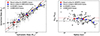 |
Fig. 7. Comparison between dynamical mass measured from galaxy kinematics with Gravsphere (Read & Steger 2017) and hydrostatic mass from X-ray gas thermodynamics using MBProj2D (Sanders et al. 2018). Black and gray points are the binned data at different radii for the selected 22 eROSITA clusters and 10 HIFLUGCS clusters from Li et al. (2023a), respectively. To demonstrate the trend, the data points are binned as medians according to their mass (left) or radii (right): red points for eROSITA clusters and blue points for HIFLUGCS clusters. Black lines indicate the one-to-one ratio, while red lines show the 40% higher dynamical mass than the hydrostatic mass. Note that the hydrostatic mass for the HIFLUGCS clusters is either from the X-COP database (Eckert et al. 2019; Ettori et al. 2019; Gadotti 2009) when available, or derived from the best-fit β model (Chen et al. 2007). |
The eROSITA clusters present a large scatter, and are distributed around the line of unity. To quantify their mean behavior, we equally divided the data points into two bins and calculated their medians. The low-mass bin shows that dynamical mass is around 40% higher than hydrostatic mass, while the high-mass bin closely aligns with the one-to-one line. For the HIFLUGCS clusters, though we have a smaller sample, but given the large richness of each cluster, we end up with more kinematic data points. We also binned the data and find a similar behavior: the dynamical mass could be as much as 40% higher than their hydrostatic mass at the low-mass end, while they are quite close toward the high-mass end. So, the two samples present consistent results. Since high mass corresponds to large radii, the same trend presented in both samples could arise from their radial variations. To examine this interpretation, we plot their dynamical-to-hydrostatic mass ratios against radius in the right panel of Fig. 7. The trend becomes more obvious. Both samples show clearly decreasing dynamical-to-hydrostatic mass ratios toward large radii. Since hydrostatic mass is known to be biased low, the lower dynamical mass could imply that the member galaxies of massive clusters are not relaxed. As such, this trend could be driven by the radial variation in the dynamical state of cluster galaxies. If confirmed with larger samples, it could be evidence that cluster galaxies at large radii are still accreting toward the center.
Since Bulbul et al. (2024) provided the weak lensing inferred mass for each cluster, we can also compare our mass measurements with those from weak lensing. However, only the total mass enclosed within R500 is available, since the weak lensing mass in Bulbul et al. (2024) was estimated using the X-ray count rate-cluster mass relation presented in Ghirardini et al. (2024). The cluster masses used to build the scaling relation are from multiple lensing surveys, including DES (Grandis et al. 2024), KiDs (Kuijken et al. 2019; Wright et al. 2020; Hildebrandt et al. 2021; Giblin et al. 2021), and HSC (Aihara et al. 2018; Li et al. 2022c). Weak lensing masses are not bias-free. Ghirardini et al. (2024) calibrated the mass using Monte Carlo simulations (Grandis et al. 2021) based on the surface mass density maps of massive halos presented in the cosmological TNG300 simulations (Pillepich et al. 2018; Springel et al. 2018; Nelson et al. 2018, 2019). Therefore, the calibration makes the weak lensing masses slightly dependent on cosmology.
Figure 8 plots the weak lensing masses against our hydrostatic masses. We do not include the comparison with dynamical masses, because for many clusters there are not sufficient member galaxies to constrain their dynamical mass profiles, making it impossible to robustly calculate the total dynamical mass or equivalent. The left panel compares the total masses measured independently with weak lensing and hydrostatic assumption. The hydrostatic masses have significantly larger uncertainties, but they consistently present lower values. We calculated the median mass of the 22 clusters, and find that weak lensing inferred mass is higher than hydrostatic mass by ∼116%. It should be noted that the two total masses correspond to different cluster radii, so the lower hydrostatic masses are partially caused by the smaller cluster radii, R500, hydro. Interestingly, the significantly higher weak lensing masses are in line with the value of σ8 measured by Ghirardini et al. (2024), which is higher than almost all previous estimates in the literature. Therefore, the larger value of σ8 might be due to the higher weak lensing masses they used.
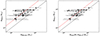 |
Fig. 8. Comparison of masses measured with weak lensing and the hydrostatic approach. Weak lensing inferred masses and radii are from Bulbul et al. (2024). The left panel compares the total masses, M500, independently inferred from these two mass proxies within their own R500 (R500, wl and R500, hydro), while the right panel compares the enclosed masses at the same radii, R500, wl. Red lines indicate the medians: M500, wl is ∼110% higher than M500, hydro, and ∼71% higher than Mhydro(R = R500, wl). Black lines are the lines of unity. |
The right panel compares weak lensing masses to the hydrostatic masses at the weak lensing inferred radius, R500, wl. Unlike the previous comparison, which is interesting in cosmology, this comparison is important for testing scaling relations and studying various dark matter models (Li et al. 2020). We find that the hydrostatic masses at R500, wl are also smaller than weak lensing masses, but the differences are much smaller, by ∼76% in terms of their medians. This is expected, given R500, wl is systematically larger than R500, hydro. The uncertainties on the hydrostatic masses are also smaller, because there are no contributions from the uncertainties on radii. The lower hydrostatic mass could be partially due to the lower temperature in eROSITA clusters with respect to Chandra and XMM-Newton observations (Migkas et al. 2024). But the influence may not be significant. Migkas et al. (2024) show that the difference in temperature is more profound in hard bands (1.5-7 keV) and less profound in soft bands (0.5–4 keV). We included even more soft bands (0.3–0.5 keV) in the image fitting, so we do not expect that the possible bias could make up the big difference in the mass measurements.
Combining the two comparisons in Figs. 7 and 8, both our dynamical and hydrostatic masses are smaller than weak lensing masses. If we trust the weak lensing mass inferred from scaling relations (Ghirardini et al. 2024), both dynamical equilibrium and hydrostatic equilibrium break down. This is possible, given that hydrostatic mass is affected by nonthermal flows and galaxies could be accreting. The question is whether they are biased by the amount we present above. Full lensing shear profiles may be required for detailed and robust investigations.
6. Radial acceleration relation from different mass estimators
Rotationally supported galaxies present an interesting correlation between centripetal acceleration, gobs, and the acceleration due to baryonic mass distributions, gbar (McGaugh et al. 2016; Lelli et al. 2017b; Li et al. 2018),
where g† = 1.2 × 10⁻¹⁰ m s−2 is the transition acceleration scale. Its universality has been tested and verified in early-type galaxies (Lelli et al. 2017a; Shelest & Lelli 2020), even with different dynamical approaches such as gravitational lensing (Mistele et al. 2024). However, it does not seem to work in galaxy clusters, as has been shown by both X-ray observations (e.g. Eckert et al. 2022; Liu et al. 2023) and gravitational lensing measurements (Tian et al. 2020). Tian et al. (2024) even found that galaxy clusters and BCGs show a consistent but distinct RAR.
We notice that these studies in galaxy clusters used a different dynamical approach with respect to disk galaxies: the former generally employs either gas thermodynamics or gravitational lensing, while the latter uses kinematics (i.e., rotation curves). To ensure consistency, Li et al. (2023a) tested the RAR in galaxy clusters using galaxy kinematics for the first time, but found similar deviations from the galaxy RAR. In particular, since galaxy distributions could be more extended than X-ray emitting gas, Li et al. (2023a) were able to explore the outskirts. However, the total accelerations in the outskirts probed by cluster galaxies are below the fiducial RAR expectations, which is contrary to those at small radii. This could be a catastrophe for the universality of the RAR. Because the observed accelerations of galaxy clusters at small radii are larger than what the RAR predicts based on observed baryonic mass (Tian et al. 2020; Eckert et al. 2022; Liu et al. 2023; Li et al. 2023a), one would have to introduce additional undetected baryons in order to achieve a universal RAR. The missing baryons could be in the form of cold gas (Milgrom 2008). It has also been argued that they could be non-baryonic, such as active neutrinos (Sanders 2003) or sterile neutrinos (Angus et al. 2008). However, the lower observed accelerations on the outskirts imply that the enclosed total mass is lower than the mass predicted by the RAR. As such, there is no room for additional baryons to compensate for the deviation at small radii, as that would require negative baryonic mass density at large radii. However, the dynamical mass measured with galaxy kinematics relies on the assumed relaxation of member galaxies, which may be broken on the outskirts, as was mentioned in Sect. 5, since galaxies could be in the process of migrating toward the cluster center. Therefore, Kelleher & Lelli (2024) propose to fit clusters without the data at radii beyond 1 Mpc.
Using the total mass estimated from different proxies, we can construct the RAR in galaxy clusters without being biased toward one sole assumption. With spherical symmetry, the total accelerations are simply given by
For different mass proxies, we have different Mtot and thereby get different gtot. In contrast, the accelerations due to baryonic mass distributions are the same, and given by
since the gas masses, Mgas, are fixed by X-ray observations, and the stellar masses are given by multiband observations (see Zou et al. 2019; Kluge et al. 2024). For galaxies that do not have measured stellar masses, we estimated their mass using the mean stellar mass-to-light ratios of the other galaxies. The total stellar mass is then the summation of the stellar masses of all member galaxies. To get the 3D stellar mass profiles, we used the normalized best-fit three Plummer’s spheres. We did not attempt to resolve the stellar mass profiles of the BCGs, given that we only explore the range at radii larger than 50 kpc.
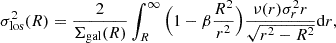
Figure 9 shows the cluster RAR constructed with gas thermodynamics, galaxy kinematics, and weak gravitational lensing. The three independent mass estimators lead to roughly the same RAR, though at R500, wl the RAR constructed with weak lensing is slightly higher than the one from the other two approaches. At small and intermediate radii, gas thermodynamics and galaxy kinematics present a RAR that is consistently higher than the fiducial line by about 0.5 dex on average. This translates into a total mass that is three times higher than expected from the RAR. It is reminiscent of the missing mass problem in modified Newtonian dynamics (MOND, Milgrom 1983). For the first time, we confirm this problem in the most robust way that does not rely on one sole assumption. The missing mass required by MOND is about two times the observed baryonic mass. Moving to larger radii, the gap narrows down to around 0.3 dex at R500, corresponding to a total mass that is two times higher. This does not mean the cumulative missing mass is decreasing, as the reference mass also increases toward large radii.
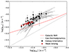 |
Fig. 9. Radial acceleration relation of galaxy clusters constructed with X-ray gas thermodynamics (gray lines), galaxy kinematics (black points), and weak gravitational lensing (red diamonds). Gray lines are truncated within 50 kpc and 2000 kpc. The weak lensing results are only available at R500 from Bulbul et al. (2024), since they were estimated using the scaling relation between weak lensing mass calibrated with simulations and X-ray count rates (with optical richness considered) (Ghirardini et al. 2024). The dotted line is the line of unity, and the solid red line is the fiducial RAR defined by disk galaxies (McGaugh et al. 2016; Lelli et al. 2017b). |
Since we calculated the hydrostatic mass up to 2 Mpc, the RARs it leads to are also more extended than those from other mass estimators. Eventually, they cross below the fiducial RAR line, implying less missing mass. However, at these large radii, whether or not hydrostatic equilibrium is valid remains uncertain. In particular, as we have shown in Fig. 8, the hydrostatic masses are lower than the masses inferred from weak lensing, which might suggest a breakdown in the assumed equilibrium. We also note that the cosmological parameter, σ8, that Ghirardini et al. (2024) derived is higher than all other estimates in the literature (see their Fig. 10). Therefore, the weak lensing mass in Bulbul et al. (2024) inferred with the scaling relation from Ghirardini et al. (2024) should be higher than the mass in other studies as well. As such, we treat the lensing results as upper limits. The current data cannot solidly confirm or rule out the possibility that adding additional baryonic mass components could make a universal RAR. We shall have to look for spatially resolved mass profiles from both weak lensing measurements and galaxy kinematics.
7. Discussion and conclusion
In this paper, we selected 22 galaxy clusters from the eRASS1 cluster catalog, requiring that there be a sufficient number of member galaxies as dynamical tracers. We measured their masses using both the thermodynamics of X-ray emitting ICM and the kinematics of member galaxies. With the X-ray data from eROSITA, we generated the images in seven energy bands for each cluster, and measured their temperature profiles, gas mass profiles, and hydrostatic mass profiles by fitting their images simultaneously. Using the photometric and spectroscopic redshifts of the member galaxies collected from the literature, we measured the projected galaxy number density profile and the line-of-sight velocity dispersion profile for each individual cluster, respectively. We parameterized the velocity anisotropy profile and the dynamical mass profile with flexible functions, and solved the Jeans equation using the MCMC approach. From the derived dynamical mass, we determined the correlation between cumulative total mass and velocity dispersion in Eq. (16), which has an rms scatter of only 0.14 dex. This correlation can be used to quickly estimate the dynamical mass profile of a galaxy cluster from velocity dispersion with an accuracy of ∼32%.
The comparison of the two mass proxies shows no systematic deviations at large radii. The roughly consistent mass measurements of galaxy clusters is not a good signal for the cosmological σ8 tension, as one would expect the problem is in the calibration of cluster mass with hydrostatic bias (Piffaretti & Valdarnini 2008; Meneghetti et al. 2010; Rasia et al. 2012, 2014; Biffi et al. 2016; Ansarifard et al. 2020; Barnes et al. 2021). Similar conclusions have been reached by Rines et al. (2016), Maughan et al. (2016), Foëx et al. (2017), Lovisari et al. (2020) using a simpler approach based on galaxy kinematics and a smaller sample. It is well known that the σ8 tension also occurs in weak lensing shear measurements, such as that from DES (Amon et al. 2022; Secco et al. 2022), KiDs (van den Busch et al. 2022), and HSC (Li et al. 2023b). Our results suggest that this tension also appears with galaxy kinematics, making it more general. Interestingly, the latest measurement using more than 5000 clusters of galaxies from eRASS1 (Ghirardini et al. 2024) shows a value of σ8 larger than almost all previous measurements, including the ones from Planck (Planck Collaboration VI 2020; Planck Collaboration VIII 2020) and WMAP (Hinshaw et al. 2013). As was noted earlier, this could be due to the higher weak lensing inferred cluster masses that they used.
One interesting trend that we notice is the slight decline in the dynamical-to-hydrostatic mass ratios toward large radii. It suggests that the inferred gravity from galaxy kinematics becomes smaller at larger radii with respect to the hydrostatic approach. This could be preliminary evidence that galaxies on the outskirts are accreting toward the center. We need more cluster galaxies on the outskirts and deeper X-ray observations to confirm this behavior with higher confidence.
Another application of robust mass measurements of galaxy clusters is to test the universality of scaling relations, such as the radial acceleration (RAR, McGaugh et al. 2016; Lelli et al. 2017b; Li et al. 2018). The RAR is an empirical relation established in galaxies. It could be an emergent phenomenon during galaxy formation, similar to the abundance matching relation (Moster et al. 2013; Behroozi et al. 2013; Kravtsov et al. 2018) and the mass-concentration relation (Macciò et al. 2008; Dutton & Macciò 2014). Navarro et al. (2017) show that the RAR can be reproduced with the aforementioned two relations using a semiempirical approach. Li et al. (2022b) show that the interplay between baryons and dark matter can significantly compress the dark matter halos of massive galaxies, leading to significant deviations to the RAR, so one might need to carefully consider the adiabatic contraction in order to reproduce the RAR and maintain stable dark matter halos simultaneously, given that massive galaxies generally experience significant baryonic compression (Li et al. 2022a; Li 2023). The RAR could also be an indicator of modified gravity, particularly MOND (Milgrom 1983), and its small scatter in disk galaxies seems to imply this interpretation (Li et al. 2018; Desmond 2023).
The key to distinguishing between these two interpretations is to test its universality, as galaxy formation is specific to galaxies, while a gravity theory should be universal in all systems. Previous studies using the hydrostatic approach (e.g. Eckert et al. 2022) and gravitational lensing (Tian et al. 2020, 2024) consistently found that galaxy clusters present higher total accelerations than what the RAR predicts with observed baryonic mass. These two approaches are fundamentally different from the one used in rotating galaxies, where the RAR was initially established. To ensure consistency, Li et al. (2023a) used a kinematic approach that employs cluster galaxies as dynamical tracers, but found similar deviations in the inner regions of clusters. In this paper, we constructed the RAR in galaxy clusters with three approaches. With a larger sample, we further confirm the missing mass problem in galaxy clusters, as is required by MOND, using three independent approaches for the first time. The particularly interesting part in Li et al. (2023a) is on the outskirts, where clusters cross below the RAR, suggesting that too much mass is predicted by the RAR. If confirmed, it would rule out a universal RAR as there would be no room for adding additional baryonic mass components in galaxy clusters. Unfortunately, the cluster sample we used in this paper does not have a sufficient number of galaxies as dynamical tracers on the outskirts, so we cannot further investigate this behavior. Future observations with SDSS-V (Almeida et al. 2023) and the 4-meter Multi-Object Spectroscopic Telescope (de Jong et al. 2012) will enable further studies.
8. Data availability
The electron number density, temperature, gas mass, and hydrostatic mass profiles for all the 22 clusters are public at https://zenodo.org/records/14169372.
Acknowledgments
This work is based on data from eROSITA, the soft X-ray instrument aboard SRG, a joint Russian-German science mission supported by the Russian Space Agency (Roskosmos), in the interests of the Russian Academy of Sciences represented by its Space Research Institute (IKI), and the Deutsches Zentrum für Luft- und Raumfahrt (DLR). The SRG spacecraft was built by Lavochkin Association (NPOL) and its subcontractors, and is operated by NPOL with support from the Max Planck Institute for Extraterrestrial Physics (MPE). The development and construction of the eROSITA X-ray instrument was led by MPE, with contributions from the Dr. Karl Remeis Observatory Bamberg & ECAP (FAU Erlangen-Nuernberg), the University of Hamburg Observatory, the Leibniz Institute for Astrophysics Potsdam (AIP), and the Institute for Astronomy and Astrophysics of the University of Tübingen, with the support of DLR and the Max Planck Society. The Argelander Institute for Astronomy of the University of Bonn and the Ludwig Maximilians Universität Munich also participated in the science preparation for eROSITA. The eROSITA data shown here were processed using the eSASS/NRTA software system developed by the German eROSITA consortium. P.L. acknowledges the support from the Alexander von Humboldt Foundation when staying at AIP where part of the work was done. A.L., M.K., E.B. V.G., C.G., and X.Z. acknowledge financial support from the European Research Council (ERC) Consolidator Grant under the European Union’s Horizon 2020 research and innovation program (grant agreement CoG DarkQuest No 101002585). Y.T. is supported by Taiwan National Science and Technology Council NSTC 110-2112-M-008-015-MY3. M.S.P. acknowledges funding of a Leibniz-Junior Research Group (project number J94/2020).
References
- Abell, G. O., Corwin, H. G. Jr, & Olowin, R. P. 1989, ApJS, 70, 1 [Google Scholar]
- Abolfathi, B., Aguado, D. S., Aguilar, G., et al. 2018, ApJS, 235, 42 [NASA ADS] [CrossRef] [Google Scholar]
- Ahumada, R., Allende Prieto, C., Almeida, A., et al. 2020, ApJS, 249, 3 [NASA ADS] [CrossRef] [Google Scholar]
- Aihara, H., Arimoto, N., Armstrong, R., et al. 2018, PASJ, 70, S4 [NASA ADS] [Google Scholar]
- Alam, S., Albareti, F. D., Allende Prieto, C., et al. 2015, ApJS, 219, 12 [Google Scholar]
- Almeida, A., Anderson, S. F., Argudo-Fernández, M., et al. 2023, ApJS, 267, 44 [NASA ADS] [CrossRef] [Google Scholar]
- Amon, A., Gruen, D., Troxel, M. A., et al. 2022, Phys. Rev. D, 105, 023514 [NASA ADS] [CrossRef] [Google Scholar]
- Anders, E., & Grevesse, N. 1989, Geochim. Cosmochim. Acta, 53, 197 [Google Scholar]
- Angus, G. W., Famaey, B., & Buote, D. A. 2008, MNRAS, 387, 1470 [CrossRef] [Google Scholar]
- Ansarifard, S., Rasia, E., Biffi, V., et al. 2020, A&A, 634, A113 [NASA ADS] [CrossRef] [EDP Sciences] [Google Scholar]
- Barnes, D. J., Vogelsberger, M., Pearce, F. A., et al. 2021, MNRAS, 506, 2533 [NASA ADS] [CrossRef] [Google Scholar]
- Battaglia, N., Bond, J. R., Pfrommer, C., & Sievers, J. L. 2012, ApJ, 758, 74 [NASA ADS] [CrossRef] [Google Scholar]
- Behroozi, P. S., Wechsler, R. H., & Conroy, C. 2013, ApJ, 770, 57 [NASA ADS] [CrossRef] [Google Scholar]
- Biffi, V., Borgani, S., Murante, G., et al. 2016, ApJ, 827, 112 [NASA ADS] [CrossRef] [Google Scholar]
- Binggeli, B., Tammann, G. A., & Sandage, A. 1987, AJ, 94, 251 [Google Scholar]
- Binney, J., & Mamon, G. A. 1982, MNRAS, 200, 361 [Google Scholar]
- Binney, J., & Tremaine, S. 2008, Galactic Dynamics: Second Edition (Princeton, NJ USA: Princeton University Press) [Google Scholar]
- Biviano, A., Murante, G., Borgani, S., et al. 2006, A&A, 456, 23 [NASA ADS] [CrossRef] [EDP Sciences] [Google Scholar]
- Biviano, A., Rosati, P., Balestra, I., et al. 2013, A&A, 558, A1 [Google Scholar]
- Bleem, L. E., Bocquet, S., Stalder, B., et al. 2020, ApJS, 247, 25 [Google Scholar]
- Bocquet, S., Dietrich, J. P., Schrabback, T., et al. 2019, ApJ, 878, 55 [Google Scholar]
- Böhringer, H., Voges, W., Huchra, J. P., et al. 2000, ApJS, 129, 435 [CrossRef] [Google Scholar]
- Böhringer, H., Schuecker, P., Guzzo, L., et al. 2004, A&A, 425, 367 [NASA ADS] [CrossRef] [EDP Sciences] [Google Scholar]
- Brunner, H., Liu, T., Lamer, G., et al. 2022, A&A, 661, A1 [NASA ADS] [CrossRef] [EDP Sciences] [Google Scholar]
- Bulbul, E., Liu, A., Kluge, M., et al. 2024, A&A, 685, A106 [NASA ADS] [CrossRef] [EDP Sciences] [Google Scholar]
- Cannon, R., Drinkwater, M., Edge, A., et al. 2006, MNRAS, 372, 425 [NASA ADS] [CrossRef] [Google Scholar]
- Chen, Y., Reiprich, T. H., Böhringer, H., Ikebe, Y., & Zhang, Y. Y. 2007, A&A, 466, 805 [NASA ADS] [CrossRef] [EDP Sciences] [Google Scholar]
- CHEX-MATE Collaboration (Arnaud, M., et al.) 2021, A&A, 650, A104 [NASA ADS] [CrossRef] [EDP Sciences] [Google Scholar]
- Coil, A. L., Blanton, M. R., Burles, S. M., et al. 2011, ApJ, 741, 8 [Google Scholar]
- Colless, M., Dalton, G., Maddox, S., et al. 2001, MNRAS, 328, 1039 [Google Scholar]
- Collins, M. L. M., Read, J. I., Ibata, R. A., et al. 2021, MNRAS, 505, 5686 [NASA ADS] [CrossRef] [Google Scholar]
- Cool, R. J., Moustakas, J., Blanton, M. R., et al. 2013, ApJ, 767, 118 [NASA ADS] [CrossRef] [Google Scholar]
- Danese, L., de Zotti, G., & di Tullio, G. 1980, A&A, 82, 322 [NASA ADS] [Google Scholar]
- Davis, M., Faber, S. M., Newman, J., et al. 2003, SPIE Conf. Ser., 4834, 161 [NASA ADS] [Google Scholar]
- de Jong, R. S., Bellido-Tirado, O., Chiappini, C., et al. 2012, SPIE Conf. Ser., 8446, 84460T [Google Scholar]
- de Jong, R. S., Agertz, O., Berbel, A. A., et al. 2019, The Messenger, 175, 3 [NASA ADS] [Google Scholar]
- De Leo, M., Read, J. I., Noël, N. E. D., et al. 2024, MNRAS, 535, 1015 [NASA ADS] [CrossRef] [Google Scholar]
- Desmond, H. 2023, MNRAS, 526, 3342 [NASA ADS] [CrossRef] [Google Scholar]
- Dey, A., Schlegel, D. J., Lang, D., et al. 2019, AJ, 157, 168 [Google Scholar]
- Donahue, M., Voit, G. M., Mahdavi, A., et al. 2014, ApJ, 794, 136 [NASA ADS] [CrossRef] [Google Scholar]
- Dutton, A. A., & Macciò, A. V. 2014, MNRAS, 441, 3359 [NASA ADS] [CrossRef] [Google Scholar]
- Eckert, D., Ettori, S., Pointecouteau, E., et al. 2017, Astron. Nachr., 338, 293 [Google Scholar]
- Eckert, D., Ghirardini, V., Ettori, S., et al. 2019, A&A, 621, A40 [NASA ADS] [CrossRef] [EDP Sciences] [Google Scholar]
- Eckert, D., Ettori, S., Pointecouteau, E., van der Burg, R. F. J., & Loubser, S. I. 2022, A&A, 662, A123 [NASA ADS] [CrossRef] [EDP Sciences] [Google Scholar]
- Ettori, S., Ghirardini, V., Eckert, D., et al. 2019, A&A, 621, A39 [NASA ADS] [CrossRef] [EDP Sciences] [Google Scholar]
- Finoguenov, A., Merloni, A., Comparat, J., et al. 2019, The Messenger, 175, 39 [NASA ADS] [Google Scholar]
- Foëx, G., Böhringer, H., & Chon, G. 2017, A&A, 606, A122 [NASA ADS] [CrossRef] [EDP Sciences] [Google Scholar]
- Foreman-Mackey, D., Hogg, D. W., Lang, D., & Goodman, J. 2013, PASP, 125, 306 [Google Scholar]
- Gadotti, D. A. 2009, MNRAS, 393, 1531 [Google Scholar]
- Genina, A., Read, J. I., Frenk, C. S., et al. 2020, MNRAS, 498, 144 [NASA ADS] [CrossRef] [Google Scholar]
- Ghirardini, V., Eckert, D., Ettori, S., et al. 2019, A&A, 621, A41 [NASA ADS] [CrossRef] [EDP Sciences] [Google Scholar]
- Ghirardini, V., Bulbul, E., Artis, E., et al. 2024, A&A, 689, A298 [NASA ADS] [CrossRef] [EDP Sciences] [Google Scholar]
- Giblin, B., Heymans, C., Asgari, M., et al. 2021, A&A, 645, A105 [NASA ADS] [CrossRef] [EDP Sciences] [Google Scholar]
- Grandis, S., Bocquet, S., Mohr, J. J., Klein, M., & Dolag, K. 2021, MNRAS, 507, 5671 [NASA ADS] [CrossRef] [Google Scholar]
- Grandis, S., Ghirardini, V., Bocquet, S., et al. 2024, A&A, 687, A178 [NASA ADS] [CrossRef] [EDP Sciences] [Google Scholar]
- Harrison, E. R. 1974, ApJ, 191, L51 [Google Scholar]
- Hildebrandt, H., van den Busch, J. L., Wright, A. H., et al. 2021, A&A, 647, A124 [EDP Sciences] [Google Scholar]
- Hilton, M., Sifón, C., Naess, S., et al. 2021, ApJS, 253, 3 [CrossRef] [Google Scholar]
- Hinshaw, G., Larson, D., Komatsu, E., et al. 2013, ApJS, 208, 19 [Google Scholar]
- Hoekstra, H., Herbonnet, R., Muzzin, A., et al. 2015, MNRAS, 449, 685 [NASA ADS] [CrossRef] [Google Scholar]
- Jones, D. H., Saunders, W., Colless, M., et al. 2004, MNRAS, 355, 747 [NASA ADS] [CrossRef] [Google Scholar]
- Jones, D. H., Read, M. A., Saunders, W., et al. 2009, MNRAS, 399, 683 [Google Scholar]
- Kelleher, R., & Lelli, F. 2024, A&A, 688, A78 [NASA ADS] [CrossRef] [EDP Sciences] [Google Scholar]
- Kluge, M., Comparat, J., Liu, A., et al. 2024, A&A, 688, A210 [NASA ADS] [CrossRef] [EDP Sciences] [Google Scholar]
- Koulouridis, E., Clerc, N., Sadibekova, T., et al. 2021, A&A, 652, A12 [NASA ADS] [CrossRef] [EDP Sciences] [Google Scholar]
- Kravtsov, A. V., Vikhlinin, A. A., & Meshcheryakov, A. V. 2018, Astron. Lette., 44, 8 [NASA ADS] [CrossRef] [Google Scholar]
- Kuijken, K., Heymans, C., Dvornik, A., et al. 2019, A&A, 625, A2 [NASA ADS] [CrossRef] [EDP Sciences] [Google Scholar]
- Lau, E. T., Kravtsov, A. V., & Nagai, D. 2009, ApJ, 705, 1129 [NASA ADS] [CrossRef] [Google Scholar]
- Lelli, F., McGaugh, S. S., & Schombert, J. M. 2017a, MNRAS, 468, L68 [NASA ADS] [CrossRef] [Google Scholar]
- Lelli, F., McGaugh, S. S., Schombert, J. M., & Pawlowski, M. S. 2017b, ApJ, 836, 152 [Google Scholar]
- Li, P. 2023, Cambridge University Press, in press [arXiv:2305.19289] [Google Scholar]
- Li, P., Lelli, F., McGaugh, S., & Schombert, J. 2018, A&A, 615, A3 [NASA ADS] [CrossRef] [EDP Sciences] [Google Scholar]
- Li, P., Lelli, F., McGaugh, S., & Schombert, J. 2020, ApJS, 247, 31 [Google Scholar]
- Li, P., Lelli, F., McGaugh, S., Schombert, J., & Chae, K.-H. 2021, A&A, 646, L13 [NASA ADS] [CrossRef] [EDP Sciences] [Google Scholar]
- Li, P., McGaugh, S. S., Lelli, F., Schombert, J. M., & Pawlowski, M. S. 2022a, A&A, 665, A143 [NASA ADS] [CrossRef] [EDP Sciences] [Google Scholar]
- Li, P., McGaugh, S. S., Lelli, F., et al. 2022b, ApJ, 927, 198 [NASA ADS] [CrossRef] [Google Scholar]
- Li, X., Miyatake, H., Luo, W., et al. 2022c, PASJ, 74, 421 [NASA ADS] [CrossRef] [Google Scholar]
- Li, P., Tian, Y., Júlio, M. P., et al. 2023a, A&A, 677, A24 [NASA ADS] [CrossRef] [EDP Sciences] [Google Scholar]
- Li, X., Zhang, T., Sugiyama, S., et al. 2023b, Phys. Rev. D, 108, 123518 [CrossRef] [Google Scholar]
- Lilly, S. J., Le Fèvre, O., Renzini, A., et al. 2007, ApJS, 172, 70 [NASA ADS] [CrossRef] [Google Scholar]
- Liu, A., Yu, H., Tozzi, P., & Zhu, Z.-H. 2016, ApJ, 821, 29 [Google Scholar]
- Liu, A., Yu, H., Diaferio, A., et al. 2018, ApJ, 863, 102 [NASA ADS] [CrossRef] [Google Scholar]
- Liu, A., Bulbul, E., Ghirardini, V., et al. 2022, A&A, 661, A2 [NASA ADS] [CrossRef] [EDP Sciences] [Google Scholar]
- Liu, A., Bulbul, E., Ramos-Ceja, M. E., et al. 2023, A&A, 670, A96 [NASA ADS] [CrossRef] [EDP Sciences] [Google Scholar]
- Lodders, K. 2003, ApJ, 591, 1220 [Google Scholar]
- Lovisari, L., Ettori, S., Sereno, M., et al. 2020, A&A, 644, A78 [NASA ADS] [CrossRef] [EDP Sciences] [Google Scholar]
- Macciò, A. V., Dutton, A. A., & van den Bosch, F. C. 2008, MNRAS, 391, 1940 [CrossRef] [Google Scholar]
- Mamon, G. A., Biviano, A., & Boué, G. 2013, MNRAS, 429, 3079 [CrossRef] [Google Scholar]
- Maughan, B. J., Giles, P. A., Rines, K. J., et al. 2016, MNRAS, 461, 4182 [NASA ADS] [CrossRef] [Google Scholar]
- McDonald, M., Benson, B. A., Vikhlinin, A., et al. 2014, ApJ, 794, 67 [Google Scholar]
- McGaugh, S. S., Schombert, J. M., Bothun, G. D., & de Blok, W. J. G. 2000, ApJ, 533, L99 [Google Scholar]
- McGaugh, S. S., Lelli, F., & Schombert, J. M. 2016, Phys. Rev. Lett., 117, 201101 [NASA ADS] [CrossRef] [Google Scholar]
- Mehrtens, N., Romer, A. K., Hilton, M., et al. 2012, MNRAS, 423, 1024 [NASA ADS] [CrossRef] [Google Scholar]
- Meneghetti, M., Rasia, E., Merten, J., et al. 2010, A&A, 514, A93 [NASA ADS] [CrossRef] [EDP Sciences] [Google Scholar]
- Merloni, A., Lamer, G., Liu, T., et al. 2024, A&A, 682, A34 [NASA ADS] [CrossRef] [EDP Sciences] [Google Scholar]
- Merrifield, M. R., & Kent, S. M. 1990, AJ, 99, 1548 [NASA ADS] [CrossRef] [Google Scholar]
- Migkas, K., Kox, D., Schellenberger, G., et al. 2024, A&A, 688, A107 [NASA ADS] [CrossRef] [EDP Sciences] [Google Scholar]
- Milgrom, M. 1983, ApJ, 270, 365 [Google Scholar]
- Milgrom, M. 2008, New Astron. Rev., 51, 906 [CrossRef] [Google Scholar]
- Mistele, T., McGaugh, S., Lelli, F., Schombert, J., & Li, P. 2024, JCAP, 2024, 020 [Google Scholar]
- Moster, B. P., Naab, T., & White, S. D. M. 2013, MNRAS, 428, 3121 [Google Scholar]
- Munari, E., Biviano, A., Borgani, S., Murante, G., & Fabjan, D. 2013, MNRAS, 430, 2638 [Google Scholar]
- Navarro, J. F., Eke, V. R., & Frenk, C. S. 1996, MNRAS, 283, L72 [NASA ADS] [Google Scholar]
- Navarro, J. F., BenÃtez-Llambay, A., Fattahi, A., et al. 2017, MNRAS, 471, 1841 [NASA ADS] [CrossRef] [Google Scholar]
- Nelson, K., Lau, E. T., & Nagai, D. 2014, ApJ, 792, 25 [NASA ADS] [CrossRef] [Google Scholar]
- Nelson, D., Pillepich, A., Springel, V., et al. 2018, MNRAS, 475, 624 [Google Scholar]
- Nelson, D., Springel, V., Pillepich, A., et al. 2019, Comput. Astrophys. Cosmol., 6, 2 [Google Scholar]
- Newman, J. A., Cooper, M. C., Davis, M., et al. 2013, ApJS, 208, 5 [Google Scholar]
- Nishizawa, A. J., Oguri, M., Oogi, T., et al. 2018, PASJ, 70, S24 [CrossRef] [Google Scholar]
- Oguri, M. 2014, MNRAS, 444, 147 [NASA ADS] [CrossRef] [Google Scholar]
- Penna-Lima, M., Bartlett, J. G., Rozo, E., et al. 2017, A&A, 604, A89 [NASA ADS] [CrossRef] [EDP Sciences] [Google Scholar]
- Piffaretti, R., & Valdarnini, R. 2008, A&A, 491, 71 [NASA ADS] [CrossRef] [EDP Sciences] [Google Scholar]
- Piffaretti, R., Arnaud, M., Pratt, G. W., Pointecouteau, E., & Melin, J. B. 2011, A&A, 534, A109 [NASA ADS] [CrossRef] [EDP Sciences] [Google Scholar]
- Pillepich, A., Nelson, D., Hernquist, L., et al. 2018, MNRAS, 475, 648 [Google Scholar]
- Planck Collaboration XXIX. 2014, A&A, 571, A29 [NASA ADS] [CrossRef] [EDP Sciences] [Google Scholar]
- Planck Collaboration XIII. 2016, A&A, 594, A13 [NASA ADS] [CrossRef] [EDP Sciences] [Google Scholar]
- Planck Collaboration XXIV. 2016, A&A, 594, A24 [NASA ADS] [CrossRef] [EDP Sciences] [Google Scholar]
- Planck Collaboration XXVII. 2016, A&A, 594, A27 [NASA ADS] [CrossRef] [EDP Sciences] [Google Scholar]
- Planck Collaboration VI. 2020, A&A, 641, A6 [NASA ADS] [CrossRef] [EDP Sciences] [Google Scholar]
- Planck Collaboration VIII. 2020, A&A, 641, A8 [NASA ADS] [CrossRef] [EDP Sciences] [Google Scholar]
- Plummer, H. C. 1911, MNRAS, 71, 460 [Google Scholar]
- Predehl, P., Andritschke, R., Arefiev, V., et al. 2021, A&A, 647, A1 [EDP Sciences] [Google Scholar]
- Rasia, E., Meneghetti, M., Martino, R., et al. 2012, New J. Phys., 14, 055018 [Google Scholar]
- Rasia, E., Lau, E. T., Borgani, S., et al. 2014, ApJ, 791, 96 [NASA ADS] [CrossRef] [Google Scholar]
- Read, J. I., & Steger, P. 2017, MNRAS, 471, 4541 [Google Scholar]
- Read, J. I., Agertz, O., & Collins, M. L. M. 2016, MNRAS, 459, 2573 [NASA ADS] [CrossRef] [Google Scholar]
- Read, J. I., Walker, M. G., & Steger, P. 2018, MNRAS, 481, 860 [NASA ADS] [CrossRef] [Google Scholar]
- Read, J. I., Mamon, G. A., Vasiliev, E., et al. 2021, MNRAS, 501, 978 [Google Scholar]
- Rines, K. J., Geller, M. J., Diaferio, A., & Hwang, H. S. 2016, ApJ, 819, 63 [NASA ADS] [CrossRef] [Google Scholar]
- Rykoff, E. S., Rozo, E., Busha, M. T., et al. 2014, ApJ, 785, 104 [Google Scholar]
- Rykoff, E. S., Rozo, E., Hollowood, D., et al. 2016, ApJS, 224, 1 [NASA ADS] [CrossRef] [Google Scholar]
- Sanders, R. H. 2003, MNRAS, 342, 901 [NASA ADS] [CrossRef] [Google Scholar]
- Sanders, J. S., Fabian, A. C., Russell, H. R., & Walker, S. A. 2018, MNRAS, 474, 1065 [NASA ADS] [CrossRef] [Google Scholar]
- Saro, A., Mohr, J. J., Bazin, G., & Dolag, K. 2013, ApJ, 772, 47 [NASA ADS] [CrossRef] [Google Scholar]
- Secco, L. F., Samuroff, S., Krause, E., et al. 2022, Phys. Rev. D, 105, 023515 [NASA ADS] [CrossRef] [Google Scholar]
- Sereno, M., Ettori, S., & Moscardini, L. 2015, MNRAS, 450, 3649 [NASA ADS] [CrossRef] [Google Scholar]
- Sereno, M., Ettori, S., Meneghetti, M., et al. 2017, MNRAS, 467, 3801 [NASA ADS] [CrossRef] [Google Scholar]
- Shelest, A., & Lelli, F. 2020, A&A, 641, A31 [EDP Sciences] [Google Scholar]
- Shi, X., Komatsu, E., Nelson, K., & Nagai, D. 2015, MNRAS, 448, 1020 [NASA ADS] [CrossRef] [Google Scholar]
- Springel, V., Pakmor, R., Pillepich, A., et al. 2018, MNRAS, 475, 676 [Google Scholar]
- Tian, Y., Umetsu, K., Ko, C.-M., Donahue, M., & Chiu, I. N. 2020, ApJ, 896, 70 [NASA ADS] [CrossRef] [Google Scholar]
- Tian, Y., Yu, P.-C., Li, P., McGaugh, S. S., & Ko, C.-M. 2021, ApJ, 910, 56 [NASA ADS] [CrossRef] [Google Scholar]
- Tian, Y., Ko, C.-M., Li, P., McGaugh, S., & Poblete, S. L. 2024, A&A, 684, A180 [NASA ADS] [CrossRef] [EDP Sciences] [Google Scholar]
- van den Busch, J. L., Wright, A. H., Hildebrandt, H., et al. 2022, A&A, 664, A170 [NASA ADS] [CrossRef] [EDP Sciences] [Google Scholar]
- van der Marel, R. P. 1994, MNRAS, 270, 271 [NASA ADS] [CrossRef] [Google Scholar]
- Vazza, F., Brunetti, G., Kritsuk, A., et al. 2009, A&A, 504, 33 [NASA ADS] [CrossRef] [EDP Sciences] [Google Scholar]
- Vikhlinin, A., Kravtsov, A., Forman, W., et al. 2006, ApJ, 640, 691 [Google Scholar]
- von der Linden, A., Mantz, A., Allen, S. W., et al. 2014, MNRAS, 443, 1973 [NASA ADS] [CrossRef] [Google Scholar]
- Wright, A. H., Hildebrandt, H., van den Busch, J. L., & Heymans, C. 2020, A&A, 637, A100 [NASA ADS] [CrossRef] [EDP Sciences] [Google Scholar]
- Zou, H., Gao, J., Zhou, X., & Kong, X. 2019, ApJS, 242, 8 [Google Scholar]
Appendix A: Additional information for the cluster sample
Alternative names and photon counts in the band of (0.2, 2.3) keV for the selected 22 clusters.
All Tables
Best-fit parameters for the temperature profile (first six parameters) and the electron number density profile (last six parameters).
Alternative names and photon counts in the band of (0.2, 2.3) keV for the selected 22 clusters.
All Figures
|
Fig. 1. X-ray image of 1eRASS J004207.0-283154 with exposure map corrected in the energy range of (0.3–7.0) keV, smoothed with Gaussian filters. Small white circles show the masked regions that were selected using the X-ray source catalog (Merloni et al. 2024) and the cluster catalog (Bulbul et al. 2024). The color bar labels the exposure-map-corrected X-ray photon counts. |
| In the text | |
|
Fig. 2. Surface brightness profiles of 1eRASS J004207.0-283154 in six different energy bands. The azimuthally averaged surface brightness in each band is compared with the total model (red lines), which is the summation of the constant background (dashed black lines) and the cluster model (solid black lines). Cluster models are truncated at 2 Mpc. |
| In the text | |
|
Fig. 3. Electron number density (top left), temperature (top right), cumulative gas mass (bottom left), and hydrostatic mass (bottom right) profiles of 1eRASS J004207.0-283154. Solid lines and shadow regions are the median values and the corresponding 68% confidence limits, respectively. Both the mean values and the uncertainties were directly extracted from their Markov chains. Notice that the profiles can also be derived using the median values in the posterior distributions of the fitting parameters in Table 2. This approach could lead to slightly different profiles from those extracted from Markov chains, but consistent within 1σ. The latter generally results in non-smooth curves. The complete figure set for all clusters is available at Zenodo. The data for these profiles are available at Github (https://pengfeili0606.github.io/data). |
| In the text | |
|
Fig. 4. Example phase-space distributions of cluster galaxies. Left panel: Spatial distribution of the member galaxies of 1eRASS J004207.0-283154 on the projected sky. Red upward triangles and blue downward triangles represent receding and approaching galaxies, respectively. Black points are galaxies without spectroscopic redshift. Right panel: Line-of-sight velocities of the member galaxies with respect to the BCG against the projected radii, rproj. Galaxies with only photometric redshift are excluded in this plot. Cluster 004207.0-283154 presents a slightly asymmetric velocity distribution of its member galaxies. This does not affect the binned velocity dispersion, as galaxies within each bin were fit using the generalized Gaussian function, which allows a variable mean velocity (see Sect. 4.2). |
| In the text | |
|
Fig. 5. Example fits to the binned cluster galaxies. Left: Galaxy surface number density profile. Points with errors are for the binned photometrically selected galaxies. The solid line is the fit profile with three projected Plummer spheres (Plummer 1911). Right: Line-of-sight velocity dispersion profile. The single point with errors is the binned velocity dispersion using spectroscopically selected galaxies, while the solid line is the expected profile based on the fit mass profile parameterized by the coreNFWtides model (Read et al. 2016). The dark and light shadow regions present 1σ and 2σ limits, respectively. In both profiles, membership probabilities of galaxies are considered when binning. To be consistent with previous figures, the example shown is from 1eRASS J004207.0-283154. |
| In the text | |
|
Fig. 6. Enclosed dynamical mass against the product σlos2rproj/G for 22 eROSITA clusters and 10 HIFLUGCS clusters from Li et al. (2023a). Note that velocity dispersion is measured at rather than within a specific radius, i.e., σlos = σlos(R = rproj)≠σlos(R < rproj), while the dynamical mass is cumulative, Mdyn = Mdyn(r < rproj), where R and r are 2D and 3D radii, respectively; rproj is the projected radius. The correlation can be described by a power law (the solid line): log Mdyn = (1.296 ± 0.001)log(σlos2rproj/G)−(3.87 ± 0.23). The total scatter is 0.14 dex (∼32%). To clarify, points with errors are the binned results at different radii, so a cluster could have more than one point. |
| In the text | |
|
Fig. 7. Comparison between dynamical mass measured from galaxy kinematics with Gravsphere (Read & Steger 2017) and hydrostatic mass from X-ray gas thermodynamics using MBProj2D (Sanders et al. 2018). Black and gray points are the binned data at different radii for the selected 22 eROSITA clusters and 10 HIFLUGCS clusters from Li et al. (2023a), respectively. To demonstrate the trend, the data points are binned as medians according to their mass (left) or radii (right): red points for eROSITA clusters and blue points for HIFLUGCS clusters. Black lines indicate the one-to-one ratio, while red lines show the 40% higher dynamical mass than the hydrostatic mass. Note that the hydrostatic mass for the HIFLUGCS clusters is either from the X-COP database (Eckert et al. 2019; Ettori et al. 2019; Gadotti 2009) when available, or derived from the best-fit β model (Chen et al. 2007). |
| In the text | |
|
Fig. 8. Comparison of masses measured with weak lensing and the hydrostatic approach. Weak lensing inferred masses and radii are from Bulbul et al. (2024). The left panel compares the total masses, M500, independently inferred from these two mass proxies within their own R500 (R500, wl and R500, hydro), while the right panel compares the enclosed masses at the same radii, R500, wl. Red lines indicate the medians: M500, wl is ∼110% higher than M500, hydro, and ∼71% higher than Mhydro(R = R500, wl). Black lines are the lines of unity. |
| In the text | |
|
Fig. 9. Radial acceleration relation of galaxy clusters constructed with X-ray gas thermodynamics (gray lines), galaxy kinematics (black points), and weak gravitational lensing (red diamonds). Gray lines are truncated within 50 kpc and 2000 kpc. The weak lensing results are only available at R500 from Bulbul et al. (2024), since they were estimated using the scaling relation between weak lensing mass calibrated with simulations and X-ray count rates (with optical richness considered) (Ghirardini et al. 2024). The dotted line is the line of unity, and the solid red line is the fiducial RAR defined by disk galaxies (McGaugh et al. 2016; Lelli et al. 2017b). |
| In the text | |
Current usage metrics show cumulative count of Article Views (full-text article views including HTML views, PDF and ePub downloads, according to the available data) and Abstracts Views on Vision4Press platform.
Data correspond to usage on the plateform after 2015. The current usage metrics is available 48-96 hours after online publication and is updated daily on week days.
Initial download of the metrics may take a while.