| Issue |
A&A
Volume 674, June 2023
Gaia Data Release 3
|
|
|---|---|---|
| Article Number | A16 | |
| Number of page(s) | 45 | |
| Section | Catalogs and data | |
| DOI | https://doi.org/10.1051/0004-6361/202245330 | |
| Published online | 16 June 2023 | |
Gaia Data Release 3
The first Gaia catalogue of eclipsing-binary candidates
1
Department of Astronomy, University of Geneva, Chemin Pegasi 51, 1290 Versoix, Switzerland
e-mail: Nami.Mowlavi@unige.ch
2
Department of Astronomy, University of Geneva, Ch. d’Ecogia 16, 1290 Versoix, Switzerland
3
Villanova University, Dept. of Astrophysics and Planetary Science, 800 Lancaster Ave, Villanova, PA, 19085
USA
4
School of Physics and Astronomy, Tel Aviv University, Tel Aviv, 6997801
Israel
5
RHEA for European Space Agency (ESA), Camino bajo del Castillo, s/n, Urbanizacion Villafranca del Castillo, Villanueva de la Cañada, 28692 Madrid, Spain
6
Sednai Sàrl, Geneva, Switzerland
7
European Space Agency (ESA), European Space Astronomy Centre (ESAC), Camino bajo del Castillo, s/n, Urbanizacion Villafranca del Castillo, Villanueva de la Cañada, 28692 Madrid, Spain
Received:
28
October
2022
Accepted:
1
March
2023
Context. Gaia Data Release 3 (DR3) provides a number of new data products that complement the early DR3 made available two years ago. Among these is the first Gaia catalogue of eclipsing-binary candidates containing 2 184 477 sources with brightnesses from a few magnitudes to 20 mag in the Gaia G-band and covering the full sky.
Aims. We present the catalogue, describe its content, provide tips for its use, estimate its quality, and show illustrative samples.
Methods. Candidate selection is based on the results of variable object classification performed within the Gaia Data Processing and Analysis Consortium. Candidates are then further filtered using eclipsing-binary-tailored criteria based on the G-band light curves. To find the orbital period, a large ensemble of trial periods is first acquired using three distinct period-search methods applied to the cleaned G light curve of each source. The G light curve is then modelled with up to two Gaussians and a cosine for each trial period. The best combination of orbital period and geometric model is finally selected using Bayesian model comparison based on the BIC. A global ranking metric is provided to rank the quality of the chosen model between sources. The catalogue is restricted to orbital periods larger than 0.2 days.
Results. Of ∼600 000 available crossmatches, about 530 000 of the candidates are classified as eclipsing binaries in the literature as well, and 93% of them have published periods compatible with the Gaia periods. Catalogue completeness is estimated to be between 25% and 50%, depending on the sky region, relative to the OGLE4 catalogues of eclipsing binaries towards the Galactic Bulge and the Magellanic Clouds. The analysis of an illustrative sample of ∼400 000 candidates with significant parallaxes shows properties in the observational Hertzsprung-Russell diagram as expected for eclipsing binaries. The subsequent analysis of a subsample of detached bright candidates provides further hints for the exploitation of the catalogue. We also address the observed lack of short-period (less than a day) systems in the Magellanic Cloud in comparison to Galactic systems. The orbital periods, light-curve model parameters, and global rankings are all published in the catalogue with their related uncertainties where applicable.
Conclusions. This Gaia DR3 catalogue of eclipsing-binary candidates constitutes the largest catalogue to date in terms of number of sources, sky coverage, and magnitude range.
Key words: binaries: eclipsing / methods: data analysis / catalogs / surveys
© The Authors 2023
 Open Access article, published by EDP Sciences, under the terms of the Creative Commons Attribution License (https://creativecommons.org/licenses/by/4.0), which permits unrestricted use, distribution, and reproduction in any medium, provided the original work is properly cited.
This article is published in open access under the Subscribe to Open model. Subscribe to A&A to support open access publication.
1. Introduction
Most stars are in binary systems and a fraction of them appear to an observer as eclipsing. Under certain conditions, these eclipsing systems allow us to determine fundamental parameters of stars, such as mass and radius, together with the orbital parameters. They provide a stringent test for stellar evolution when the two stars are in wide systems, while they are laboratories for many physical processes when the two stars interact with one another. Some eccentric systems can also serve as a test of the theory of general relativity thanks to the determination of their apsidal motion. In addition, when one of the components is oscillating and provides suitable conditions to perform asteroseismology, the system provides an independent determination of stellar parameters and the possibility to test the asteroseismic scaling relations. Clearly, eclipsing binaries are exceptionally interesting objects for astronomy. Still, the number of well-studied cases is relatively small. For example, the catalogue of well-studied systems presented by Southworth (2015) contains 1701 binaries, based on an initial compilation of 45 eclipsing binaries by Andersen (1991).
With the advent of large-scale multi-epoch ground-based photometric surveys, pioneered by the microlensing search ‘Expérience pour la recherche d’objets sombres’ (EROS1 Renault et al. 1998), the ‘Massive compact halo object’ experiment (MACHO Alcock et al. 1997), and the ‘Optical gravitational lensing experiment’ (OGLE2 Udalski et al. 1992), the opportunities to find eclipsing binaries increased dramatically. The precursor of Gaia, HIPPARCOS, already provided an all-sky survey of eclipsing binaries (ESA 1997). The number of eclipsing binaries was rather limited, namely about 900 were found among 11 597 detected variables (from 118 218 monitored stars), yet ∼30% of these were new candidates. Before the present Gaia Data Release 3 (DR3), the largest catalogue specifically dedicated to eclipsing binaries came from the OGLE4 survey team with the publication of 40 204 sources in the Large Magellanic Cloud (LMC, Pawlak et al. 2016), 8401 sources in the Small Magellanic Cloud (SMC, Pawlak et al. 2016), and 450 598 sources towards the Galactic Bulge (Soszyński et al. 2016). In parallel, multiple other large-scale multi-epoch surveys provide additional opportunities, with automated classification of their variable stars. Such is the case, for example, for (number of eclipsing binaries given in parenthesis) the Trans-Atlantic Exoplanet Survey (TRES; Devor et al. 2008, 773), the All Sky Automated Survey (ASAS; Pojmanski 2002; Pigulski et al. 2009, 1055 and 180, respectively), the Lincoln Near-Earth Asteroid Research survey (LINEAR; Palaversa et al. 2013, 2700), the EROS2 survey (Kim et al. 2014, ∼45 600), the CATALINA survey (Drake et al. 2017, 23 312), the Asteroid Terrestrial-impact Last Alert System survey (ATLAS; Heinze et al. 2018, ∼110 000), and the Zwicky Transient Facility survey (Chen et al. 2020, ∼420 000). The catalogue of variable stars made available by the American Association of Variable Star Observers (AAVSO) through their Variable Star Index (VSX) database also provides a wealth of data for the study of eclipsing binaries (Watson et al. 2006).
Space missions dedicated to exoplanet searches provide another source of data for the study of eclipsing binaries. Their strengths come from continuous, high-cadence observations on long timescales combined with the high photometric precision that can be obtained from space. Catalogues dedicated to eclipsing binaries from these missions include Kirk et al. (2016) for Kepler (2878 candidates including ellipsoidal variables) and Prša et al. (2022) from the Transiting Exoplanet Survey Satellite (TESS; 4584 eclipsing binaries), although these are limited in terms of sky coverage and/or brightness range.
The Gaia space mission from the European Space Agency (ESA) offers a new opportunity to study eclipsing binaries. Launched at the end of 2013, this all-sky survey started its nominal mission in July 2014 (Gaia Collaboration 2016). Among the strong points of the mission for variability analysis, we can mention, in addition to its well-known astrometric capabilities, the large dynamical range reached in stellar brightness, from a few magnitudes to fainter than 20 mag, the specific scanning law leading to irregularly sampled time series, and the quasi-simultaneity (within tens of seconds) of the observations in G photometry, GBP and GRP spectrophotometry, and RVS (Radial Velocity Spectrometer) spectroscopy. Data products based on 34 months of astrometry and photometry data were released in the early DR3 (EDR3 in December 3, 2020; Gaia Collaboration 2021; Riello et al. 2021). These were complemented with numerous additional data products in DR3 (June 13, 2022; Gaia Collaboration 2023b), including variability catalogues for more than ten million variable objects (Eyer et al. 2023).
This paper presents the first Gaia catalogue of eclipsing binaries, published as part of Gaia DR3. It is the largest catalogue of its kind to date, with more than two million candidates. A balance was reached between completeness and purity. The selection of the eclipsing binaries starts with the classification of variable objects performed within the Gaia Processing and Analysis Consortium (DPAC) as described in Rimoldini et al. (2023), followed by a specific eclipsing-binary module that automatically selects a geometric two-Gaussian model (see Mowlavi et al. 2017) and orbital period based on the G light curves. Subsequently, there is a final filtering step on various statistical parameters. The GBP and GRP time series were not used. The eclipsing-binary processing pipeline is described in Sect. 2. In particular, the section describes candidate selection, orbital period search, the two-Gaussian model used to fit the morphology of the G light curves, and the procedure implemented to automate the selection of the best model and orbital period, as well as to derive uncertainties for the determined parameters. Section 2 also details the content of the catalogue. Recommendations for catalogue exploitation using published parameters are given in Sect. 3. The quality of the catalogue is then addressed in Sect. 4, with an estimate of catalogue completeness and an investigation of the new Gaia candidates. Illustrative samples of candidates with good parallaxes are presented in Sect. 5, with a specific application to the period–eccentricity analysis of bright candidates. Section 6 ends the main body of the text with a summary and conclusions.
Additional content is presented in four Appendices. Appendix A presents an analysis of the various types of two-Gaussian models used to fit the eclipsing-binary light curves. Appendix B elaborates on the eccentricity proxy that can be derived from the light curve. Appendix C presents additional figures referenced in the main body of the text. Appendix D completes the acknowledgments.
2. The catalogue
The 2 184 477 sources published in table gaiadr3.vari_eclipsing_binary (under Variability in the Gaia archive) constitute the Gaia DR3 catalogue of eclipsing binaries. The candidates were selected considering a mixture of various criteria with the goal of reaching a relatively good degree of completeness while limiting the level of contamination. The list of sources in this catalogue is essentially the same as the list of variables identified as eclipsing binaries in the general Gaia DR3 classification table vari_classifier_result (variability type ECL; for details, see Rimoldini et al. 2023). Small differences nevertheless exist between the two tables. Nineteen sources are present in the classification table but are not in the catalogue of eclipsing binaries. Periods and light-curve characterisation are therefore not available for these sources. Conversely, the catalogue of eclipsing binaries contains 140 candidates not listed in the classification table because of a post-processing step of the classification table that modified the label of a small fraction of sources. In this paper, we restrict the analysis to the catalogue of eclipsing binaries.
From the two million eclipsing-binary candidates, 86 918 were further processed within the DPAC to derive orbital solutions. The results are published in table gaiadr3.nss_two_body_orbit (under Non-single stars in the Gaia archive), with nss_solution_type=‘EclipsingBinary’. We refer to Siopis et al. (in prep.) for a presentation of that table. In addition, 155 of them have combined photometric + spectroscopic solutions (identified in the table with nss_solution_type=‘EclipsingSpectro’). We refer to Gaia Collaboration (2023a) for further information.
The distribution on the sky of the eclipsing-binary candidates from the catalogue is shown in Fig. 1. The G light curves contain between 16 and 259 cleaned field-of-view (FOV) measurements, depending on the sky position according to the Gaia scanning law. For each candidate, an orbital period is provided in the catalogue, together with a geometrical characterisation of its G light curve and a global ranking that ranges from 0.4 to 0.84 (Eqs. (4) and (5) in Sect. 2.2), where a higher value indicates a better light curve characterisation. Figure 2 gives the G magnitude distribution for the full catalogue (in black) and for the subsamples with the highest (> 0.6, in green) and lowest (< 0.5, in red) global rankings.
 |
Fig. 1. Sky-density map of the Gaia catalogue of eclipsing binaries in Galactic coordinates. The map is colour-coded according to the colour scale shown to the right of the figure. |
 |
Fig. 2. Distribution of G magnitude of the full sample (black histogram) and of the samples with global ranking larger than 0.6 (filled green histogram) and smaller than 0.5 (red spiked histogram). The abscissa scale is truncated at the lower side for improved visibility. |
The eclipsing-binary pipeline is presented in Sects. 2.1–2.3. The input to the pipeline is briefly described in Sect. 2.1. The geometrical characterisation of the light curves is detailed in Sect. 2.2, and our post-pipeline selection criteria are presented in Sect. 2.3. The content of the catalogue is summarised in Sect. 2.4.
2.1. Eclipsing-binary pipeline input
The eclipsing-binary module that generated the candidates published here is part of the variability pipeline consisting of several stages, which are described in Eyer et al. (2017, 2023). After a general variability detection performed on all Gaia sources, variable source candidates go through a classification stage (Rimoldini et al. 2023). Sources classified as eclipsing binaries are then fed to our eclipsing-binary module.
Not all sources initially classified as eclipsing binaries are published in DR3. An initial selection keeps only sources that are brighter than 20 mag in G, that have at least 16 cleaned FOV measurements in their G light curves, and for which the skewness in the G time series is larger than −0.2. This constitutes ∼20 million sources. The eclipsing-binary pipeline then processes the G light curves (as described in Sect. 2.2), and a final selection further filters out sources according to period and folded light curve properties (see Sect. 2.3).
2.2. Light-curve characterisation
For each eclipsing-binary candidate, a geometric model of its G-band light curve is constructed by fitting up to two Gaussians and one cosine to the cleaned G-band time series. The Gaussian components are designed to model the geometrical shape of the light curve of the eclipses, and the cosine component is designed to model the geometrical shape of an ellipsoidal-like variability. The model is used to characterise the geometry of the light curve, select the most probable orbital period based purely on the photometry, and provide a ranking among all sources.
The ‘two-Gaussian’ model is introduced in Sect. 2.2.1, and its derived parameters are described in Sect. 2.2.2. The period-search method is then presented in Sect. 2.2.3, followed in Sect. 2.2.4 by the procedure used to estimate the uncertainty on these parameters. Our final strategy to select a light-curve model for each source is given in Sect. 2.2.5.
2.2.1. Two-Gaussian model parameters
The geometrical model fitted to the G light curve consists of up to two Gaussians and a cosine. The model can contain any combination of these three components, and not all are necessarily present; it is referred to as a ‘two-Gaussian’ model irrespective of the number of components it eventually contains. A full description of the model is given in Mowlavi et al. (2017), to which we refer for more details. Below, we summarise the model components and associated parameters.
A Gaussian component k is defined as
where φ is the orbital phase, that is (observation time − reference time T0) modulo (orbital period), and μk, dk, and σk are the Gaussian parameters (phase location of the centre, depth in magnitude, and width in phase, respectively) of the first (k = 1) and second (k = 2) Gaussian, when present. A schematic representation of a model with two Gaussians mimicking a well-detached binary system is shown in the top panel of Fig. 3, while the middle panel illustrates the case of a tighter system modelled with two overlapping Gaussians. We note that there are not always two Gaussians in the models and, when there are two, the first Gaussian is not necessarily the deepest of the two.
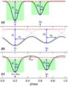 |
Fig. 3. Schematic representation of the two-Gaussian model parameters used in Eq. (3) to fit folded light curves of eclipsing binaries. The ordinate represents magnitude in reverse order. Three cases are shown with their primary eclipses (arbitrarily) located at phase 0.2. Case (a) illustrates the modelling of a well-detached eccentric system using two non-overlapping Gaussians. Case (b) shows a very tight circular system modelled with two overlapping Gaussians. Case (c) represents a tight circular system with an out-of-eclipse ellipsoidal variation modelled with a cosine component. The red dashed horizontal line in each panel indicates the value of the constant C in Eq. (3). The green areas delimit the eclipse durations. The thin black dotted lines in the middle and bottom panels show the individual Gaussian and/or cosine components of the two-Gaussian models. The thick black solid lines show the resulting two-Gaussian models. |
When a Gaussian component is included, its mirror functions at phases below zero and above one are automatically added to take into account the contribution of the tails of the Gaussian function from adjacent phases due to the periodicity of the eclipses (see Eq. (2) of Mowlavi et al. 2017). This is necessary for a correct inclusion of wide Gaussians.
The cosine component, when present, has a period equal to half of the orbital period, and is given by
where Aell is the amplitude of the cosine function. If there are any Gaussian components, μell is either equal to μ1 or μ2, depending on whether the cosine is centred on the first or second Gaussian component, respectively. If the model contains only a cosine, μell is fitted to the data as an independent parameter.
When all the components are present, the model writes
where C is the reference level. The list of model types according to the number of components, and the number of parameters for each model type are summarised in Table 1. We note that this model is adequate to represent eccentric systems only in the absence of a cosine component, and that reflection –which would be described with a cosine component with a period equal to the orbital period– is not included in this first Gaia catalogue of eclipsing binaries.
Types of geometric models fitting the G light curves.
All parameters necessary to reconstruct the geometric model are published in the catalogue, and are summarised in Table 2. The model component parameters are given in field names prepended with ‘geom_model_’. The orbital period is given as a frequency (to which a frequency uncertainty can be associated; see Sect. 2.2.4), which is derived as described in Sect. 2.2.3. The phase is computed based on this period and on the reference time that is also published.
Data fields in the Gaia DR3 table of eclipsing binaries (Gaia DR3 table vari_eclipsing_binary), with their units (Col. 2), the mathematical symbol used in this paper (if used, Col. 3), and a short description (Col. 4).
2.2.2. Derived geometric model parameters
In addition to the ‘two-Gaussian’ model parameters, several parameters are derived from the geometric model and published in the catalogue in field names prepended with ‘derived_’ (see Table 2). These derived parameters give eclipse characteristics (phase location, phase duration, depth) based on the geometric model as given by Eq. (3). The deepest and second-deepest eclipse information is stored in the ‘primary’ and ‘secondary’ eclipse fields, respectively. We reiterate that the underlying Gaussian model components 1 and 2 have no specific order.
Derived eclipse parameters are only provided in association with a Gaussian component. A dip in the folded light curve that results from a cosine component and that has no associated Gaussian does not have derived eclipse parameters. Therefore, models containing a cosine and a Gaussian, for example, only have one set of derived eclipse parameters. Only the ‘derived_primary_*’ fields are then filled in the catalogue. Likewise, purely cosine models have no derived parameters.
The derived eclipse phase locations are obtained by starting at the centre of the Gaussian (1 or 2) and identifying the closest zero-derivative (flat) point in the light curve, which is not necessarily located at the same positions as the centres of the Gaussians if they are not offset by 0.5 in phase or when there is an ellipsoidal component. The derived eclipse depth is defined as the distance between the model value at the derived primary or secondary eclipse phase and the brightest model value, and the derived eclipse duration in phase is defined as 5.6 σk, with σk being defined in Eq. (1), with a maximum of 0.4 (see Mowlavi et al. 2017). These last two definitions equally apply for models with and without an ellipsoidal component.
2.2.3. Period search
The orbital period is obtained in two steps. First, a list of up to 22 candidate periods is established from the G light curve as described in this section. Two-Gaussian models are then fitted to the light curve for each of these periods, and the best model is selected as described in Sect. 2.2.5. The period of this best model is the orbital period published in the catalogue together with the best model parameters.
Due to the variety of eclipsing-binary light-curve geometries, we combined the results of three different period-search methods to identify the list of candidate periods. The three methods are the Generalised Least-Squares (Heck et al. 1985; Cumming et al. 1999; Zechmeister & Kürster 2009), the Phase Dispersion Minimisation (Jurkevich 1971; Stellingwerf 1978; Schwarzenberg-Czerny 1997), and the String Length (Lafler & Kinman 1965; Burke et al. 1970) methods. The choice of these three different methods is based on earlier internal tests on HIPPARCOS (ESA 1997) eclipsing binaries, which showed that the highest level of correct period recovery is found in the union of this ensemble. In the DR3 catalogue of eclipsing binaries, the unweighted procedure has been used in all cases because the observations in the eclipses are fainter than their corresponding out-of-eclipse values (and their uncertainties consequently larger), and they would therefore be down-weighted in a weighted procedure. Periodograms are computed using these three methods in the frequency range between 0.005 and 15 d−1 (spanning 1.6 h to 200 d) using a fixed frequency step of 10−5 d−1.
The two most significant peaks in each of the three periodograms are then gathered in a list of candidate frequencies, to which half and twice their values are added for all three methods, as well as one-third and four times their values for Generalised Least-Squares. In this way, a set of 22 candidate periods is constructed, some of which might overlap between the different methods.
2.2.4. Model parameter uncertainties
Due to the often low duty cycle of eclipsing signals (e.g., down to an adopted minimum of three observations in eclipse), estimations of the uncertainties in our models can be inherently imprecise. As formal errors from the least-squares fit do not capture any modelling errors, we opted for the jackknife method to get a sense of the uncertainties around our best-fit-solution parameters.
For this data release, we implemented a Jackknife method with non-robust mean and variance estimates (Wall & Jenkins 2003). This means that, in order to estimate the uncertainties of the best-fit-model parameters p (including frequency, reference level, and derived parameters) of a source with N observations Xi = 1 → N, we refit the model N times, where each time one of the observations Xi is left out. Generally, for each refit, this recovers a similar, but not identical parameter solution pi of which the variance
(Eq. (6.20) in Wall & Jenkins 2003) is used to populate the uncertainty estimate. Because instances of the N jackknife refits can cause non-convergence, a minimum of 30% converged solutions was required to estimate the uncertainties. If more than 70% of the refits failed, the model is rejected from the list of model candidates for the given source (see Sect. 2.2.5). Even though most Jackknife solutions converged, some included some anomalously large values, which is reflected in some of the published uncertainties. Alternatively, in some cases, the Jackknife samples showed insufficient variation for a good uncertainty estimate, resulting in some near-zero uncertainty estimates. We intend to improve upon this point in DR4 by implementing a more robust estimate of the variance.
The Jackknife method described above allows us to estimate the uncertainties of not only the geometric model parameters, but also of the frequency, reference level, and derived parameters. These uncertainties are generally more informative (and larger) than the formal errors obtained from a simple linear covariance estimation at the best-fit parameter set, because the latter does not include any modelling errors and assumes that observation uncertainties are correctly estimated.
As the frequency is among the most important parameters, we applied more stringent checks and bounds on its estimated Jackknife uncertainty. We set frequency_error = MAX(frequency_error, 0.001/time_duration_g_fov) where time_duration_g_fov is the duration between the first and last observations, as published in the gaiadr3.vari_summary table. Additionally we identified that for frequency_error × time_duration_g_fov > 0.6, no correct period is recovered in our literature cross-match. Therefore, we rejected all models with a value above this limit. These lower and upper bounds on the frequency uncertainty forb, err respectively correspond to 0.1% and 60% phase deviations2 at the last cycle of the observations with the given period Porb = 1/forb.
The uncertainties on all model parameters are published in the catalogue in field names appended with ‘_error’. These include the geometrical model parameters as well as the orbital frequency and derived parameters.
2.2.5. Model-selection strategy
For each of the candidate periods identified in Sect. 2.2.3 (up to 22 in number), seven two-Gaussian models are fitted to the G light curve by considering all possible combinations of the two-Gaussian components, including a simple constant model in order to make a proper model comparison against a non-variable model. This results in a list of up to 154 model candidates per source, considering the six model types listed in Table 1 and the additional constant model. The models are then cleaned and sorted according to their Bayesian information criterion (BIC) score (Feigelson & Babu 2012, Eq. (3.54)), which allows us to compare model fits for all combinations of the candidate periods and geometric models; we then select the best model. Each of these steps is briefly described in the following paragraphs.
In the first, cleaning step, models that have component parameters that we deem non-physical are removed from the list of model candidates. Visual inspection of earlier iterations of our pipeline on Gaia data revealed that the geometric model parameters may model features that we deem non-physical. This is the case when two Gaussian components are too close to each other. We therefore remove a model from the list of model candidates if the derived primary and secondary eclipse locations are less than 0.08 apart in phase in order to avoid stacking Gaussians on the same eclipse. We also remove models with one Gaussian if its width is larger than 0.4 in phase, as well as models with one Gaussian and a cosine component if the Gaussian width is larger than 0.4 in phase (as a Gaussian of this width is partially degenerate with the ellipsoidal component). The pipeline also checks the uncertainties of the geometric model parameters, and rejects models that have uncertainties greater than 10 mag for the reference level (C in Eq. (3)) or for the cosine amplitude (Aell), or greater than one for the phase locations (μ1, μ2) or widths (σ1, σ2) of the Gaussians. No condition is given on the uncertainties of the Gaussian depths as this quantity can be unconstrained for well-detached systems with narrow eclipses.
After this first pruning of models, we order the list of remaining model candidates according to their BIC score. In the adopted BIC convention, a higher BIC score identifies a better model fit to the data by taking into account the number of free parameters in each model and giving a higher weight to models that have a smaller number of parameters. We then retain all models that have a BIC score within 30 of the highest BIC score. All these model candidates are considered to be equivalently good at this point. This list is then filtered according to several exclusion criteria. We remove: the constant model that was added to the list of models, if it remains in the list of model candidates; models that have a phase coverage of less than 0.6 (the phase coverage is computed by binning the phase-folded data into ten bins and counting the fraction of filled bins); and models that have less than three observations in an eclipse. If multiple models survive at this point, a pre-defined model ranking is used to select the model with the highest rank according to the model ranking indicated in Table 1. It must be noted that this model ranking inevitably introduces priors in the model selection. For example, circular systems with two equal-depth eclipses will be favoured over eccentric systems displaying only one eclipse (these two cases differ by a factor of two in their orbital periods). If no candidate model remains in the final list, the source is removed from the catalogue.
2.3. Post-pipeline source filtering and model ranking
In this first Gaia catalogue of eclipsing binaries, the output of the pipeline underwent a large variety of verification and validation checks that led to the application of additional filters outlined here. The first filter concerns the periods found in the time series; it requires that the internal second-best model (see Sect. 2.2.5) have a period compatible with the one found in the best model (i.e. with period ratios equal to 0.5, 1, 1.5, or 2). Additional criteria further consider the Abbe value on the folded light curves in combination with various frequency limits and global ranking criteria. Finally, sources with periods smaller than 0.2 d were removed because of the larger occurrence in DR3 of aliases at these small periods.
In order to compare the models of all sources in the catalogue, a global ranking is computed based on the fraction of variance unexplained (FVU). This quantity is defined as the ratio of the variance of the residuals to the variance of the signal, and is given by
In this equation, Gobs, i is the ith measurement of the NG observations in the G time series, Gmodel, i is the value of the model at that time, and  the mean G magnitude. A global ranking that ranges between zero and one is then derived using a linear transformation of the base ten logarithm of the FUV, given by
The constants in this equation are empirically derived to map the log(FVU) values in the range from zero to one. Our last source filter uses this global ranking. Only sources with a global ranking larger than 0.4 are published in the catalogue.
2.4. Catalogue content
The data fields published in the catalogue are listed in Table 2. They include the orbital frequency, the geometrical model parameters of the G-band light curve, the parameters derived from the model, the uncertainties on these parameters, and the global ranking. Orbital frequencies are published rather than orbital periods for consistency with the internal model parameterisation and subsequent uncertainty estimates by the Jackknife method.
The model type is one of the six possible combinations of two Gaussian functions and a cosine function, which are listed in Table 1, together with the number of sources present in the catalogue for each type. All model parameters are named with a prefix ‘geom_’. The numbering of the first and second Gaussians follows the order of dip detection in the pipeline, and does not necessarily correspond to an order where the deepest Gaussian would be Gaussian one and the shallowest Gaussian would be Gaussian two.
The two-Gaussian model represents a purely geometrical description of the light-curve morphology and is not intended to model the physical properties of the binary system. However, from the two-Gaussian model, estimates of the phase locations, durations, and depths of the primary and secondary eclipses are derived by identifying the deepest and second-deepest dips, respectively, in the model light curve (see Sect. 2.2.2). These quantities are published in the catalogue with data field names prepended with ‘derived_’.
As mentioned in Sect. 2.2.4, the current uncertainty estimation is not robust against outlying samples in the Jackknife method, and can therefore lead to arbitrarily high uncertainties in some cases. This explains the presence in the table of unrealistically large estimates of the errors on some parameters. In addition, values above 3.4E38 have been converted to NULL values, as they cannot fit in a numeric float type in the database. As a result, there are 1131 sources that have NULL values for geom_model_gaussian1_depth_error, 824 sources that have NULL values for geom_model_gaussian2_depth_error, 776 sources that have NULL values for derived_primary_ecl_depth_error, and 1145 sources that have NULL values for derived_secondary_ecl_depth_error, despite these same sources having non-NULL values for the quantities to which the errors are associated.
3. Catalogue usage
3.1. Light-curve models
The automated procedure that processes the data of the two million Gaia eclipsing-binary candidates finds the best two-Gaussian-model fit to the G light curves. As stressed in Sect. 2.4, the model represents a purely geometrical description of the light-curve morphology. The model parameters are not necessarily linked to physical properties of the binary system –despite a good description of light-curve geometry–, because of, for example, a lack of phase coverage, spurious feature identifications in the light curves, or a potentially incorrect period determination. However, the model parameters can in a large number of cases inform us about the physical properties of the eclipses (depth, duration, eccentricity) and the ellipsoidal variability (amplitude).
A detailed analysis of the light-curve models is presented in Appendix A, where the light curves are classified in samples that have two, one, or no Gaussian components, with a naming convention starting with 2G, 1G, or 0G, respectively, and with a letter E added when an ellipsoidal component is present. In addition, groups 2G and 2GE are further subclassified depending on model parameters by adding a postfix to the group name of -A, -B, -C, -D, -X, -Y, or -Z. The definitions of the groups are given in Table A.1. This basic classification is only meant to guide the user on the catalogue content and various types of light-curve morphologies. The main types of binary systems expected in each of these groups are given in Table 3 (see Appendix A.6 for a discussion), with the distribution in each group detailed in Table 4. In this section, we present examples of known eclipsing binaries, all available in the catalogue of Avvakumova et al. (2013).
The overwhelming majority of G light curves are modelled with two Gaussians (94% of sources in the catalogue; see Table 1). Among these, two-thirds have strictly two Gaussian components. The most obvious eclipsing-binary configuration whose light curve can be modelled in this way is that of well-detached systems with constant out-of-eclipse light. The two Gaussians have similar widths, but not necessarily similar depths. In Appendix A, such well-detached systems define Sample 2G-A (285 320 candidates). The G folded light curve of V614 Ven in this sample is displayed in the top panel of Fig. 4. We reiterate that only the G data were used to produce the results published in the DR3 catalogue of eclipsing binaries. The GBP and GRP time series are nevertheless available in the DR3 Gaia archive. The GBP and GRP folded light curves of V614 Ven are shown in the bottom panel of Fig. 4.
 |
Fig. 4. Folded light curves of V614 Ven. Top panel: G light curve. The two-Gaussian model is superposed as a dotted line. The green areas indicate the derived eclipse durations. Bottom panel: GBP and GRP light curves (blue and red dots, respectively), shifted by a value equal to their respective median magnitudes as written in the top of the panel. The GRP light curve is plotted on top of the GBP one, the former therefore hiding the latter when the measurements are at the same ordinate. The dotted model and green areas shown in the bottom panel are the ones from the G light curve shifted to match zero median magnitude. The Gaia period, global ranking, and the light-curve classification (in brackets; see text) are given in the title of the figure after the Gaia DR3 ID and GCVS name. |
Tighter systems in which one or both stars fill their Roche lobes can also display light curves reminiscent of detached systems (e.g., Pojmanski 2002; Paczyński et al. 2006) and therefore be found in Sample 2G-A. This can, for example, happen when the star that fills its Roche lobe is much fainter than its companion such that the induced ellipsoidal variability is below the detection limit (depending on the photometric precision of the instrument). The secondary eclipse would then also be much shallower than the primary eclipse. These features typically characterise Algo-type binaries, which are understood to result from a past mass-transfer episode. Algol itself is not available in Gaia DR3 because of its brightness (2.1 mag in V), but the example of SW Cyg, a A2Ve+KI system (Malkov 2020), is given in the top panel of Fig. 53. The absence of detected out-of-eclipse variability therefore does not necessarily imply a well-detached system. The variety of binary configuration in Sample 2G-A is also attested by the depth ratio distribution shown in blue in the top panel of Fig. 6. The histogram covers all values from close-to-zero to one, with two main peaks, one at small ratios below 0.2, and another at depth ratios close to one.
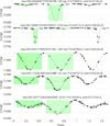 |
Fig. 5. Same as the top panel of Fig. 4, but for additional eclipsing binaries for which the G light curves are modelled with only two Gaussians. From top to bottom: SW Cyg, V745 Cep, 1687 Aql, NS Cam, and KS Eri. |
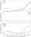 |
Fig. 6. Distribution of the derived eclipse-depth ratio (secondary over primary) for the various samples with two Gaussians in their light-curve models without (top and middle panels) or with (bottom panel) an ellipsoidal component, as labelled in the panels (see text). The histograms are area-normalised. |
Some light curves are modelled with a very narrow primary Gaussian and a wide secondary. In the subclassification presented in Appendix A, these light curves are gathered in Sample 2G-D. The secondary Gaussians of these cases are, on average, much shallower than their primary Gaussian, as shown in Fig. 6 (second panel, cyan histogram). When the primary eclipse is very narrow, the detection of the secondary eclipse may be challenging, which is due for example to insufficient measurements in the eclipse and/or an overly shallow secondary eclipse. The probability that the pipeline fails to correctly detect the secondary, or that the orbital period is incorrect, is therefore much greater than for Sample 2G-A candidates. The second example in Fig. 5 displays a case in Sample 2G-D, V745 Cep classified as a semi-detached system in Avvakumova et al. (2013), where both Gaussians correctly identify the eclipses.
Tight systems are generally modelled with two Gaussians and a cosine to account for the ellipsoidal out-of-eclipse variability. These light curves belong to either Sample 2GE-A or 2GE-B in Appendix A, depending on the amplitude of the ellipsoidal variability. Sample 2GE-A (162 630 sources) contains candidates with small to medium amplitudes of 2 Aell < 0.11 mag, while Sample 2GE-B (265 276 sources) has 2 Aell > 0.11 mag. Sample 2GE-A is similar to Sample 2G-A except for the additional cosine component. Four such examples are shown in Fig. 7, with increasing ellipsoidal amplitude (relative to primary eclipse depth) from the top to the third case, and with a total eclipse in the fourth case. The two famous eclipsing binaries β-Lyr and W UMa, the prototypes of the classical EB- and EW-type eclipsing binaries, respectively, belong to Sample 2GE-B; their light curves are shown in Fig. 8.
 |
Fig. 7. Same as top panel of Fig. 4, but for sources with light curves modelled with two Gaussians and a cosine of small to medium amplitude. From top to bottom: AO Ser, DN Cas, MU Cyg, and HN Cas. |
 |
Fig. 8. Same as top panel of Fig. 4, but for sources with light curves modelled with two Gaussians and a cosine of large amplitude. From top to bottom: β Lyr and W UMa. |
Very tight systems, including semi-detached systems with large ellipsoidal variability, in-contact systems, or systems with a common envelope, have their light curves modelled in several ways using a two-Gaussian model. The most common way consists of two wide overlapping Gaussians of similar width. These systems form Sample 2G-B, which contains 834 093 sources. The Gaussians are located at a phase separation of about 0.5 from each other. The majority of these sources have similar eclipse depths, as seen by the green histogram in Fig. 6 (top panel). 1687 Aql is one example, shown in the third panel of Fig. 5. An example in Sample 2G-B with significantly unequal eclipse depths, NS Cam, is shown in the fourth panel.
A small fraction of candidates modelled with two wide overlapping Gaussians have non-equal Gaussian widths. This feature can reproduce the asymmetries present in the light curves of tight systems. Such candidates form Sample 2G-C (24 081 sources). The distribution of eclipse-depth ratio for this sample is very similar to that of Sample 2G-B (red dotted histogram in Fig. 6, top panel). An example is given in the bottom panel of Fig. 5 with KS Eri, a binary system displaying the O’Connell effect.
In less than 4% of the DR3 eclipsing-binary candidates, the light curve is modelled without a second Gaussian. These belong to samples 1G and 1GE depending on whether or not the model contains a cosine component. The lack of a secondary Gaussian can be due to several factors. One is a lack of eclipse phase coverage. Such is the case for KN And (Fig. 9, top panel) and V379 Per (second panel). The absence of a second Gaussian can also be due to the presence of a cosine component that is sufficient to model the secondary eclipse. This is the case for RZ Col, shown in the third panel of Fig. 9.
 |
Fig. 9. Same as top panel of Fig. 4, but for sources with light curves modelled with only one Gaussian (KN And, top panel), one Gaussian and a cosine (V379 Per in second panel and RZ Col in third panel), or only a cosine (DU Car, bottom panel). No green area is displayed for eclipses that are not modelled with a Gaussian component in the light-curve model. |
Finally, a single cosine may be sufficient to model a light curve. Candidates for which this is the case form Sample 0GE (36 227 sources), and DU Car illustrates this case in Fig. 9 (bottom panel).
About one-fifth of the ∼2 million sources that contain two Gaussians in their light-curve model do not fall in one of the above categories, namely Samples 2G-A, 2G-B, 2G-C, 2G-D, 2GE-A, 2GE-B, 1G, 1GE, or 0GE. These sources form three additional categories, namely 2G-X, 2G-Y, and 2GE-Z, depending on their model parameters. We refer to Appendix A for more details. The probability that their model components reflect physical configurations of the eclipsing binaries is much lower than for the other groups, and they are to be investigated on a case-by-case basis. Examples of nevertheless correct cases in each of these three samples, and where the Gaia period agrees with the literature period, are shown in Fig. 10.
 |
Fig. 10. Same as top panel of Fig. 4, but for additional sources with light curves modelled with at least two Gaussians. From top to bottom: AE Mon, V444 Cyg and RU Gem. |
In conclusion, the two-Gaussian model is a powerful tool for studying the two million eclipsing-binary candidates published in Gaia DR3. The classification provided in Appendix A gives some insight into the types of binary system, keeping in mind that each group defined in that Appendix contains a variety of different light-curve morphologies. In addition, there is an inherent degeneracy in light-curve morphology between different types of binary systems that makes it impossible to discriminate between them solely based on G photometry. The case of detached and semi-detached systems is mentioned above. From the 119 semi-detached systems listed in Malkov (2020), 95 are present in the DR3 catalogue and 74 have Gaia periods compatible within 5% with the values gathered by this latter author. Among these 74 sources, 60 have an ellipsoidal component in their two-Gaussian model (36 in Sample 2GE-A, 19 in 2GE-B, and 5 in 1GE), and 14 do not (5 in 2G-A, 6 in 2G-B, 1 in 1G, and 2 in 2G-X).
3.2. Global ranking
The global ranking is directly linked to the fraction of the variance unexplained by the two-Gaussian model through Eq. (5). As such, it informs us about the reliability of an eclipsing-binary candidate, with a larger global ranking corresponding to a better fit to the light curve, and therefore to a more reliable eclipsing-binary candidate. However, a poor global ranking does not necessarily imply a false detection, as it relies on the assumption that the functions included in the model can adequately describe the light curve of an eclipsing binary. The two-Gaussian model will fail to recognise an eclipsing binary if some physics dominating the shape of the light curve is not modelled by these functions. Such would be the case, for example, for ellipsoidal variables on an eccentric orbit including heartbeat stars; for close binaries featuring a reflection effect (which translates into a cosine function with a period equal to the orbital period); or for short-period, tight binaries that have asymmetric light curves due for example to spots. These and other such cases may even be excluded from our catalogue if their rank falls below 0.4. Sources in the catalogue with a low global ranking will therefore necessitate additional investigation in order to confirm and characterise their binary nature, and may contain systems with light-curve geometries that cannot be modelled with the two-Gaussian components. Sources with a high global ranking, on the other hand, have a high probability of being eclipsing binaries.
The distribution of the global ranking is shown in Fig. 11 for the full catalogue (black histogram). It ranges from 0.40 to 0.84, with a maximum of the distribution around 0.51. Candidates with low global rankings are, on average, fainter than the ones with high global rankings. This is illustrated by the green and red histograms in Fig. 2, where the sample with rankings higher than 0.6 (filled green histogram) peaks around 17.3 mag, while sources with rankings lower than 0.5 (red hatched histogram) are located at much fainter magnitudes around 19 mag. This apparent relationship mainly results from the fact that faint sources have larger epoch G uncertainties than bright sources, which in turn generally leads to poorer eclipsing-binary light-curve characterisation, and hence lower rankings. Figure 12, which plots the signal-to-noise ratio (S/N) in G (std_dev_over_rms_err_mag_g_fov in the Gaia archive) versus global ranking generally supports this explanation.
 |
Fig. 11. Distribution of the global ranking of DR3 EB candidates. The full sample is displayed in thick grey, with the candidates therein that have a cross-match with known eclipsing binaries in the literature shown in thin black. The sample with positive parallax uncertainties better than 15% is displayed in thick green, with the candidates therein with a literature cross-match shown in thin cyan. |
 |
Fig. 12. Density map of the S/N of the G time series (standard deviation of the measurements divided by the root mean square of their uncertainties) of all eclipsing-binary candidates versus their global ranking. The density in the map is colour coded according to the colour scale shown to the right of the figure. |
The histograms of the global ranking for the various samples discussed in the previous section are shown in Fig. 13. The largest global rankings, on average, are found in samples whose model components have a higher probability of representing physical features (eclipses and ellipsoidal variability). These are samples 2G-A and 2G-B without an ellipsoidal component (respectively blue and green distributions in the top panel of Fig. 13), and samples 2GE-A and 2GE-B with an ellipsoidal component (respectively blue and green distributions in the bottom panel). We note that the presence of an ellipsoidal component leads to a higher global ranking, on average, as the ellipsoidal variability is well defined by a cosine (in circular orbits). Notable is the histogram of Sample 2G-C (dashed red histogram in the top panel), which peaks to lower global rankings than the 2G-A, 2G-B, 2GE-A, and 2GE-B samples, despite their generally good light curves. Global-ranking-limited selections should take this into account to avoid their exclusion. Samples 2G-X, 2G-Y, and 2GE-Z, on the other hand, which contain light-curve models with components that are predominantly unrelated to physical features, have small rankings.
 |
Fig. 13. Same as Fig. 6, but for the global ranking. The histograms of the samples are displayed in two panels as labelled in the panels. |
Additional insight into the global-ranking distributions is provided in Appendix A.6. Figure A.27, in particular, shows the distribution of the global ranking versus G magnitude for each sample.
3.3. Orbital periods
The distribution of the orbital periods of the full sample is shown in Fig. 14 (black histogram) on a linear scale for the number of sources in the top panel and on a logarithmic scale in the bottom panel. In half of the cases, the periods result from the ‘string length’ method, while the ‘phase dispersion minimisation’ and ‘generalised least squares’ methods each provide the periods for ∼25% of the sample (see Sect. 2.2.3). Peaks are observed at specific periods above about five days, and especially above 20 days. These structures result from a combination of period-search artefacts and potential scan-angle-dependent signals related to the Gaia instrument calibration and mission properties, such as the scanning law and orientation (Holl et al. 2023). Such structures are significantly more scarce in the sample with global rankings larger than 0.60, as shown by the green filled histogram in Fig. 14. Figure 15 gives a more detailed view of the period distribution versus global rankings. At global rankings larger than 0.54, unexpected peaks are visible mainly at periods longer than 30 days, and more specifically around –in decreasing order of importance– 53.7 d, 107.2 d, and 34.1 d. These structures are far more scarce in sources with a global ranking below 0.54. Instead, structures are visible between 4 and 50 days. At global rankings below ∼0.5, the 6h alias due to the spacecraft rotation and its related 12h alias become significant. The reader is referred to Holl et al. (2023) for an in-depth discussion on the origin and identification of scan-angle-dependent signals that can result in the observed spurious peaks in the DR3 period distributions. The impact of such signals on the eclipsing-binary candidates is addressed in Sect. 3.5.
 |
Fig. 14. Distribution of the orbital periods of the DR3 eclipsing-binary candidates. The full sample is displayed with a black line, and the sample with global ranking higher than 0.6 is shown in green. The top panel shows the number of counts per bin on a linear scale, while the bottom panel shows them on a logarithmic scale. |
 |
Fig. 15. Density map of the orbital period versus global ranking of the DR3 eclipsing-binary candidates. |
The period distributions for the various samples discussed in Sect. 3.1 are shown in Fig. 16 (solid lines). The samples are grouped in three categories. Wider systems (on the mean) are shown in the top panel (samples 2G-A, 2GE-A, 2G-D, 1G). The periods span all values, with a peak at around 1 day and an extended tail above 20 days. The observed period distributions reflect the real distribution of these mainly detached eclipsing binaries convolved with the (complex) selection function resulting from the Gaia eclipsing-binary identification, period determination, and light-curve-modelling procedures. We also note the presence of the alias peak at the six-hour rotation period. The excess is predominant in Sample 2G-D, which contains very narrow primary Gaussians (red histogram), while it is absent in Sample 2GE-A (green histogram) where the presence of a small- to medium-amplitude ellipsoidal component (2 Aell < 0.11 mag) in the light-curve model better constrains the period.
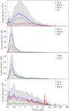 |
Fig. 16. Period distributions of various samples according to their two-model parameters as labelled in the panels (see text). The filled grey histograms represent the combined samples in each panel. |
The periods of tighter systems are shown in the second (samples 2G-B, 2GE-B, 1GE) and third (samples 0GE, 2G-C) panels. They have narrower distributions than the well-detached systems, peaking at ∼0.35 days (second and third panels in Fig. 16). The tighter systems include tighter detached, contact, and ellipsoidal systems. No excess is observed at ∼0.25 d in the period distributions of these systems.
The last category shown in the bottom panel gathers samples 2G-X, 2G-Y, and 2GE-Z, whose light-curve model components are not necessarily linked to physical features of the binary system. This category contains about one-fifth of the full catalogue. The period distributions reveal much more complex structures. Many peaks are observed over the full range of periods, with a predominance at 0.25 days and above 20 days. These distributions support the conclusions drawn in Sect. 3.1, which point out the requirement for confirmation of their periods and the nature of the eclipsing binaries in these samples.
Additional insight into the period distributions is provided in Appendix A.6. Figure A.26, in particular, shows the distribution of periods versus G magnitude for each sample, and Fig. A.28 the distribution of periods against number of measurements, which is further discussed below.
3.4. Number of measurements
The catalogue-construction procedure described in Sect. 2 limits the impact of the number of G measurements on the catalogue output. In particular, no specific structure is visible in the sky distribution of the eclipsing-binary candidates (Fig. 1), despite the strongly non-uniform sky distribution of NG due to the Gaia scanning law (Fig. C.6). Likewise, no dependence of the global ranking on NG is visible from the full catalogue sample shown in Fig. 17.
 |
Fig. 17. Density map of the number of good measurements in the G band versus global ranking. |
There are nevertheless effects of NG on the period distribution, as shown in the top panel of Fig. 18. Alias structures are visible when NG ≲ 30 in a wide range of periods below about 15 days, and at all NG values above this period limit. One recommendation could therefore be to limit the sample to candidates with NG > 30 and to those in given period ranges for studies involving orbital periods. However, these period alias structures are likely related to the so-called scan-angle-dependent signals explained in Sect. 3.5 and can to a large degree be identified using the ripd, G statistic discussed there. However, these criteria must be adapted to each two-Gaussian model type. To help the user to set suitable filtering criteria, the NG versus period distributions for the groups identified in Sect. 3.1 are shown in Fig. A.28. We note, for example, that groups 2GE-A, 2GE-B, and 1GE are not affected by aliases even at NG < 30, which is because of the presence of an ellipsoidal component in their light curves. For these candidates, no restriction on NG is necessary. The case of group 2G-A is interesting as it includes well-detached wide systems. Its NG versus period distribution shown in the top panel of Fig. A.28 suggests a filter NG > 30 should be predominantly applied at periods above 4 days. The same is true for group 2G-B. These groups have a double-peaked NG distribution (a peak around 23 and another one around 43), with a majority of candidates in the second peak. The light curves of two candidates from Group 2G-A are shown in Fig. 19, one with a small number of measurements and yet a high global ranking of 0.60, and another with a large number of measurements but low ranking of 0.44. In contrast, groups 2G-X and 2G-Y have a larger concentration of candidates with low NG values, and display many alias structures. These groups were identified in Sect. 3.1 as containing a majority of candidates with unphysical light-curve model components. These are only examples of application; users are encouraged to apply adequate NG-period filters depending on their case studies.
 |
Fig. 18. Number of good measurements in the G band versus period plane. Top panel: density map. Bottom panel: median value of the global ranking in each cell of the figure, colour-coded according to the colour scale shown to the right of the panel. |
 |
Fig. 19. Same as Fig. 4 for two additional candidates in group 2G-A. Top panel: candidate with a low number of measurements in G and high global ranking. Bottom panel: candidate with a large number of measurements in G and low global ranking. |
Finally, the global ranking is dependent on the location in the NG-versus-period plane, as shown in the bottom panel of Fig. 18. However, here too, the distribution of global ranking varies significantly as a function of the choice of light-curve model. This is shown in Fig. A.29. Groups 2GE-A and 2GE-B have high global rankings overall, while groups 2G-X, 2G-Y, and 2GE-Z have poor rankings overall. Groups 2G-A and especially 2G-B have a clear period limit above which the ranking becomes poor. At intermediate periods, in [∼2, ∼10] d for 2G-A and [∼0.5, ∼1.5] d for 2G-B, the ranking increases, on average, with increasing number of observations.
3.5. Photometric signal from source asymmetry
Holl et al. (2023) identified that asymmetric flux distributions, that is, non-point-like sources, such as partially or unresolved multiple sources and galaxies, can result in a scan-angle-dependent signal in the Gaia G-derived epoch photometry. A variety of statistics were proposed to identify sources affected by such signals, of which the Spearman correlation ripd, G is one of the most powerful. A value around 0 means the source is likely unaffected by such a signal, while a value close to 1 means it is very likely to be affected (values towards −1 would be troubling in the same way, but do not systematically occur). This parameter is available as spearman_corr_ipd_g_fov in table gaia_dr3.vari_spurious_signals in the Gaia archive and is used hereafter to decipher the approximate number of sources in our eclipsing-binary sample that might be affected.
The distribution of ripd, G versus global ranking is shown in Fig. 20. The bulk of the sources has a ripd, G distribution around 0.1, with a dispersion that slightly increases with decreasing global ranking. However, a small fraction of the sources (6%) have ripd, G values above 0.6, pointing to an origin of the photometric variability linked to an asymmetry of the source flux distribution. In principal, the asymmetry could result from the presence of an unresolved binary, especially since we are dealing with binaries. At first glance, the fact that these sources have low global rankings might seem inconsistent with this interpretation. But a high correlation means that there exists a clear signal when phase folding the light curve as function of the scan angle (see Holl et al. 2023, for details), and not with the best-fit period. As the two-Gaussian model used here does not have any degrees of freedom to (additionally) fit for this scan-angle-dependent signal, a high ripd, G will generally result in large residuals and therefore a low global ranking. The statistics are shown in Table 4. We see that the groups that have the largest percentage of sources with ripd, G > 0.6 are 2G-Y (25%), 2G-X (18%), and 2GE-Z (8%), with an overall level of contamination of ‘good’ sources estimated to be ∼5% by comparing this to the counts for ripd, G values below −0.4 (the peak of the distribution is at ∼0.1). These three groups are the ones identified in Sect. 3.1 as requiring confirmation of their binary nature, which is fully consistent with their model-fit being negatively affected by a potential scan-angle signal.
 |
Fig. 20. Density map of the ripd, G correlation (providing an indication of the possible strength of a scan-angle-dependent signal in the photometric time series) versus global ranking of the full catalogue. |
The scan-angle-dependent signals also manifest themselves at specific spurious periods identified in Holl et al. (2023), which again appear consistent with the main period clusters identified in Fig. A.28 per group, and are summarised for the full catalogue in Fig. 21. The ripd, G versus period distributions for each individual group is displayed in Fig. A.30. These figures will help the users to apply proper filters to their samples according to the ripd, G, period and Group to which the sources belong.
 |
Fig. 21. Same as Fig. 20, but versus orbital period and with a more restricted ordinate range for better visibility. |
4. Catalogue quality
We assess the quality of our catalogue by comparison of our results with literature data based on the Gaia DR3 cross-matches presented in Gavras et al. (2023). For the Gaia DR3 catalogue of eclipsing binaries, there are 606 393 cross-matches. The main surveys and number of cross-matched sources are listed in Table 5. The largest number of cross-matches relates to the ZTF survey (42%), followed by OGLE4 (17%), ASAS-SN (14%), ATLAS (10%), CATALINA (8%), and PS1 (5%). The remaining 4% of cross-matches come from a variety of sources not detailed here.
Surveys cross-matched with the Gaia DR3 catalogue of eclipsing binaries.
The statistics of the Gaia DR3 cross-matches with the literature are reported in Table 6. The first set of two rows (labelled ‘All’ in the XMs column) gives the statistics for the sample of all cross-matches, irrespective of whether or not the source is classified as an eclipsing binary in the literature. The table lists the number of sources, the number of sources that have a period reported in the literature, and the number of sources for which the literature period is compatible with the Gaia period, either directly (1:1 ratio, see Sect. 4.1) or within a factor of one or two (1:1, 1:2 or 2:1 ratios). The second two-row set (labelled ‘EB’) then provides the same statistics, but only for the subsample of cross-matches that are also classified as eclipsing binaries in the literature. The last two-row set (labelled ‘non-EB’) finally gives the statistics for the complementary subsample of cross-matches that are classified in the literature in a variability type other than eclipsing binary.
Some statistics on the period comparison between the Gaia DR3 catalogue of eclipsing binaries and literature data.
Table 6 shows that the great majority (87%) of the Gaia DR3 eclipsing binaries cross-matched with literature data are also identified in the literature as eclipsing binaries. This is a good score given the fact that classification of large catalogues is performed through automated procedures, a process that necessarily introduces a fraction of incorrect classifications that will impact the comparison between two independent catalogues. Among the non-EB crossmatches, we note that the Gaia eclipsing-binary candidates cross-matched with non-eclipsing binaries in the literature include 1205 candidates classified as ellipsoidal variables in OGLE4.
In Sect. 4.1, we first compare our periods with the ones found in the literature. Questions surrounding the completeness and purity of the catalogue are then addressed in Sects. 4.2 and 4.3, respectively.
4.1. Orbital periods
Almost all Gaia DR3 eclipsing-binary candidates that have a cross-match in the literature also have a period published in the literature (99% of them; see Table 6), allowing a direct comparison with our periods. To do so, for any given source, we evaluate the phase deviation rP, lit at the end of the observation obtained when adopting the literature period Plit instead of the Gaia period PGaia. This is computed by multiplying the relative difference between the literature and Gaia periods by the number of cycles during the observation, and is given by
where ΔT is the duration of the G light curve. Its cumulative distribution is shown in a grey-filled histogram in Fig. 22 for cross-matches that are classified as eclipsing binaries in the literature. More than 85% of the sources have a phase deviation less than 0.5 at the last cycle of their observation. The histogram also shows that when this is not the case, the value of rP, lit is much larger than 1, indicating a significant difference between the Gaia and literature periods. We therefore consider the Gaia and literature periods to be equal when rP, lit < 1. The number of such sources is reported in the fourth column of Table 6. If we also include sources with Gaia periods that are half or twice the literature periods (replacing Plit by 0.5 Plit or 2 Plit in Eq. (6)), the percentage of sources with compatible Gaia and literature data increases to 93% (fifth column of the table).
 |
Fig. 22. Cumulative distribution of the phase deviation rP, lit at the end of the observation obtained when adopting the literature period Plit instead of the Gaia period PGaia (see Eq. (6)). The sample of Gaia eclipsing-binary candidates that are also classified as eclipsing binaries in the literatures is shown by the filled grey histogram, and the sample which has literature cross-matches but with a classification other than eclipsing binary in the literature is shown by the red histogram. |
In contrast, the Gaia period is equal to that in the literature for less than 6% of sources not classified as eclipsing binaries in the literature (red histogram in Fig. 22 and fourth column in Table 6). Interestingly, this number increases to 32% when considering compatible periods (Plit/PGaia ≃ (0.5, 1, 2) in the table). This can easily be understood if the sources have sinusoidal-like light curves. The detected period can then easily be equal to twice the orbital period if it is an eclipsing binary or ellipsoidal variable, and a survey may pick either one of these periods.
The comparison between Gaia and literature periods is shown in Fig. 23. The upper panel displays the periods of the cross-matches classified as eclipsing binaries in both Gaia DR3 and the literature. These are distributed as expected, with the presence of (mainly) PGaia:Plit = 1:2, 2:1, and 2:3 ratios in addition to the overwhelming 1:1 cases. Alias features are also seen. The distribution of the Gaia eclipsing-binary candidates cross-matched with sources classified as non-eclipsing binaries in the literature, on the other hand, reveals the imprints of the underlying literature catalogues in the distributions of Plit (bottom panel in the figure). At literature periods below 1 day, we see the imprint of ∼31 600 sources from PS1_RRL_SESAR_2017 (Sesar et al. 2017), while the main contribution at literature periods above 20 days comes from ∼17 200 sources from ATLAS_VAR_HEINZE_2018 (Heinze et al. 2018). The former catalogue targets RR Lyrae variables, while the cross-matches in the latter catalogue were assigned the tailored ‘OMIT’ classification type in Gavras et al. (2023) in order to gather sources whose classification in the literature was considered to be ‘too generic, uncertain, or with insufficient variability characterisation’ (see Gavras et al. 2023). Heinze et al. (2018) mainly assigned –in decreasing order of number of cross-matches with our eclipsing binaries– the types NSINE (pure sine wave fit, but noisy data), SINE, or MSINE (modulated sine wave). However, these cross-matches not classified as eclipsing binaries in the literature or considered uncertain by Gavras et al. (2023) are a minority of the full sample of cross-matches.
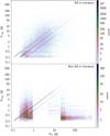 |
Fig. 23. Gaia period versus literature period for all Gaia DR3 eclipsing-binary candidates that have a cross-match in the literature. Top panel: candidates also identified as eclipsing binaries in the literature. Bottom panel: candidates not classified as eclipsing binaries in the literature. The imprints of literature catalogues are visible in the distributions of Plit (see text). |
In summary, the Gaia periods are compatible with literature periods in about 85% of cases. This includes cases where the literature period is twice or half the Gaia period.
4.2. Completeness of the Gaia catalogue
To estimate the completeness of our catalogue, we compare it with the OGLE4 catalogues of eclipsing binaries, which are available, which are available for the LMC and SMC (Pawlak et al. 2016) and for the Galactic Bulge (Soszyński et al. 2016). The sky distribution of the Gaia DR3 eclipsing binaries towards the LMC and Galactic Bulge is displayed in the top panels of Figs. 24 and 25, respectively, and the distributions of the OGLE4 eclipsing binaries in the second panels. Sources in common in Gaia DR3 and OGLE4 catalogues are shown in the third panels.
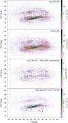 |
Fig. 24. Sky distributions (density maps) in equatorial coordinates of eclipsing-binary candidates around the LMC. The panels show, from top to bottom, Gaia DR3 candidates, OGLE4 candidates, the Gaia-OGLE4 cross-matches (2 arcsecs radius), and the new Gaia candidates with respect to OGLE4. Sources highlighted by filled circles in the bottom panel have their G light curves displayed in Figs. 31 and 32; they are located in the bar of the LMC for the cyan markers and outside the bar for the blue markers. The orange area delineates the subregion of the sky used in the text to compute the fraction of Gaia new candidates towards the LMC. |
Estimation of the completeness of the Gaia catalogue relative to the OGLE4 catalogues is achieved in two steps. We first restrict the OGLE4 catalogues to sources present in the full Gaia DR3 archive, with a cross-match search radius of one arcsecond. The statistics are given in Table 7. Gaia cross-matches are found for almost all OGLE4 eclipsing binaries in the LMC and SMC, but for only 87% of the OGLE4 sources in the Galactic Bulge (420 321/473 798 in Table 7). The 13% OGLE4 sources from the Bulge that are not in the Gaia archive are all very red faint sources with OGLE I magnitudes mainly between 18 and 20.5 mag. Their sky distribution is shown in Fig. 26.
 |
Fig. 26. Same as Fig. 24, but for OGLE4 sources in the Galactic Bulge that have no source counterpart in the Gaia DR3 archive. |
Number of OGLE4 eclipsing binaries towards the LMC, SMC, and Galactic Bulge.
We then limit the OGLE4 samples to sources brighter than 20 mag in G to comply with the input magnitude selection of the Gaia eclipsing binaries (see Sect. 2.1). The final OGLE4 samples contain 35 392, 7843, and 315 523 sources in the LMC, SMC, and Galactic Bulge4, respectively (see Table 7).
From these OGLE4 samples, 28% are present in the Gaia catalogue of eclipsing binaries (36% had we considered 19 mag as the faintest limit for both OGLE4 and Gaia catalogues). The recovery rates are larger in the Magellanic Clouds than in the Bulge, as detailed in Table 7, reaching 48% in the SMC while being 26% in the Bulge. An investigation of the 72% missing OGLE4 sources reveals that ∼45% were excluded from the initial selection (see Sect. 2.1, with ∼40% not being classified as eclipsing binaries and another ∼5% having less than 16 measurements in their G light curves, mainly in the Bulge). The remaining ∼27% of missing sources were further filtered out from the final selection procedure (Sect. 2.3).
A small fraction of the missing OGLE4 eclipsing binaries that were not classified as eclipsing binaries in Gaia DR3 are present in other variability tables published in DR3 (tables gaiadr3.vari_* in the Gaia archive). These consist of 2195 short-timescale variables, 426 binary candidates with a compact companion, 384 long-period variables, 89 main sequence oscillators, 32 rotation modulation variables, 31 Cepheids, and one active galactic nucleus.
In summary, the completeness of the Gaia catalogue of eclipsing binaries amounts to between 25% and 50% depending on the sky region when compared to the OGLE4 catalogues of eclipsing binaries. The missing OGLE4 sources were excluded from the Gaia catalogue at candidate-selection steps in our processing pipeline. As a general remark, we also recall that systems whose light curves cannot be modelled with the two-Gaussian model will lead to low global rankings and be excluded from our catalogue if the ranking falls below 0.4 (see Sect. 3.2). A significant increase in the number of eclipsing-binary candidates is therefore expected for the next Gaia release, DR4.
4.3. New Gaia candidates
In this section, we investigate the Gaia eclipsing-binary candidates that are not present in the OGLE4 catalogues of eclipsing binaries, using the LMC and Galactic Bulge regions as test cases. For this purpose, two sky areas well covered by the OGLE4 surveys are defined towards these regions: the rectangle area 70o < RA < 90o and −73o < Dec < −65o towards the LMC, and the parallelogram area with corners (RA, Dec) = (269o, −37o), (275o, −30o), (275o, −23o), (265o, −37o) towards the Galactic Bulge. These are shown by the orange borders in Figs. 24 and 25, respectively. The statistics on Gaia and OGLE4 sources in these regions are summarised in Table 8. There are 26 020 Gaia eclipsing-binary candidates towards the LMC and 96 199 sources towards the Galactic Bulge. More than half of these are new relative to the OGLE4 catalogues (53% in the LMC and 65% in the Galactic Bulge; see Table 8).
Number of Gaia DR3 eclipsing-binary candidates in selected sky areas of the LMC and Galactic Bulge.
The sky distribution of the new Gaia candidates towards the LMC is shown in the bottom panel of Fig. 24; they are mostly concentrated in the bar, where the sky density of stars is highest. The magnitude distribution of these sources peaks around 19 mag in G (red histogram in the top panel of Fig. 27), similarly to the magnitude distribution of the full Gaia sample in the defined sky area (black histogram). In contrast, the magnitude distribution of the Gaia–OGLE4 cross-match sample reveals a plateau between ∼18.5 and ∼19.5 mag (green histogram). The origin of this plateau is unclear, as the full OGLE4 sample in the defined sky area shows a continuously increasing distribution of G up to 20 mag (not shown here). We checked that the new faint sources are not contaminated by the potential presence of a nearby brighter eclipsing binary.
 |
Fig. 27. Median G magnitude distributions of Gaia eclipsing binaries in specific regions of the sky. Top panel: sky region towards the LMC shown in Fig. 24. Bottom panel: sky region towards the Galactic Bulge shown in Fig. 25. The black histograms show all Gaia DR3 eclipsing-binary candidates in the given sky area. The sources among them that have or do not have a cross-match (2 arcsec radius) with the OGLE4 catalogue of eclipsing binaries are shown by the green and red histograms, respectively. The blue histograms are the distributions of sources with no OGLE4 cross-match but a cross match with eclipsing-binary candidates identified in other surveys. The abscissa range is truncated on the bright side for greater visibility. |
The global rankings of the new Gaia candidates (with respect to OGLE4) towards the LMC are, on average, much lower than those of the Gaia–OGLE4 cross-matches. This is seen from the global-ranking distributions shown in the top panel of Fig. 28, in red for the new candidates and in green for the cross-match sample. As the majority of these new Gaia candidates are faint and lie in crowded regions of the LMC, the eclipsing-binary signature in the G light curves can be mingled with variability of non-astrophysical origin. This would explain their low global rankings. The fraction of new Gaia candidates is much smaller if we limit the samples to sources with larger global rankings. In a sample limited to global rankings larger than 0.5, for example, the fraction of new Gaia candidates towards the LMC is three times less than in the full sample (17% new candidates with respect to OGLE4, compared to 53% considering all global rankings; see Table 8). It is interesting to note that the global-ranking distribution of the Gaia candidates not in OGLE4 but identified as eclipsing binaries in other surveys (blue histogram in the Fig. 28) peaks at values between those of the new candidates and those of the Gaia–OGLE4 cross-match sample.
Figure 29 investigates a potential non-astrophysical origin of the detected variability using the Spearman correlation ripd, G introduced in Sect. 3.5, where we mention that a large value of ripd, G can result from the binary nature of the source. However, visual binaries in dense regions of the sky can also lead to asymmetric source images. The distribution of ripd, G versus period for the sources in the LMC also identified as eclipsing binaries in OGLE4 (top panel of Fig. 29) does not display an excess of sources at large values of ripd, G, as expected. The distribution of the new Gaia candidates (middle panel) shows some artefacts with large ripd, G values at known alias periods that are most probably the result of visual binaries, but these constitute only a small fraction of the sample of new Gaia candidates.
 |
Fig. 29. Same as Fig. 21, but for sources in the LMC. Top panel: sources detected as eclipsing binaries by OGLE4. Middle panel: new candidates with respect to OGLE4. Bottom panel: new candidates with respect to OGLE4 in the red clump. |
The distribution of the new Gaia candidates towards the LMC in the colour–magnitude diagram is shown in Fig. 30 together with the distribution of the Gaia candidates that have an OGLE4 cross-match. A comparison of the two distributions reveals two features. The first is the larger GBP − GRP colour dispersion in the sample of new Gaia candidates (upper-left panel in Fig. 30) compared to that in the cross-matched sample (upper-middle panel), most visible at the faint end of the main sequence. The correctness of the red colours must therefore be verified, as the GBP and GRP values of these faint sources may be affected by residual background estimates and/or multiple source blending in the BP and RP spectra. The BP+RP flux excess factor C available in the Gaia archive (phot_bp_rp_excess_factor in the gaia_source table) provides a handy tool for this purpose (assuming G is correct). This quantity, denoted C by the authors, evaluates the excess of the integrated BP and RP fluxes in comparison with the G flux (Riello et al. 2021); it is shown versus GBP − GRP in the bottom-left panel of Fig. 30. While many sources are seen to have an excess factor between 1.1 and 1.2, as expected, a non-negligible fraction of them have excess factors significantly above 1.2. This is particularly true for the red sources. These large excess factors lead to unreliable GBP and/or GRP magnitudes, and can therefore be at the origin of the large colour dispersion observed at the faint end of the main sequence. We note that the value of C of the cross-matched sources has a much cleaner distribution around the expected values (bottom-middle panel of Fig. 30). The G values, on the other hand, should be reliable, within the uncertainties expected at the faint magnitudes.
 |
Fig. 30. Colour–magnitude (top row) and BP+RP flux excess factor versus colour (bottom row) diagrams of the Gaia eclipsing binaries in the sky area towards the LMC shown in Fig. 24. Left panels: new Gaia eclipsing-binary candidates with respect to the OGLE4 catalogue of LMC eclipsing binaries. Middle panels:Gaia sources with a cross-match (2 arcsec radius) with the OGLE4 catalogue. Right panels: Gaia candidates having no cross-match with the OGLE4 candidates but a cross-match with EB candidates in other surveys. The colour of each bin is proportional to the number of counts per bin according to the colour scales shown to the right for each row. Sources highlighted by filled circles have their G light curves displayed in Figs. 31 and 32; they are located in the bar of the LMC for blue circle markers and outside the bar for cyan diamond markers. The axes ranges have been truncated for greater visibility. |
Visual inspection of the G light curves of the new Gaia candidates provides confidence that at least one-third of them are genuine eclipsing binaries. Moreover, about 17% of these new Gaia candidates towards the LMC with no OGLE4 cross-match are classified as eclipsing binaries in other surveys, using cross-matches from Gavras et al. (2023). These sources were mainly identified from the EROS2 survey by Kim et al. (2014). Eleven examples of good light curves from the Gaia new candidates not in the OGLE4 catalogue are shown in Figs. 31 and 32. Figure 31 shows sources located outside the bar of the LMC. Two of them, sources Gaia DR3 4651581458546544000 and Gaia DR3 4655269942119876864, are also referenced as eclipsing binaries in EROS2. The light curves in Fig. 32 are from sources located in the bar of the LMC. Their sky positions are indicated in Fig. 24, in blue for the sources outside the LMC bar and in cyan for those inside the bar. All 11 light curves show a variety of geometric morphologies typical of eclipsing binaries.
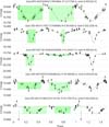 |
Fig. 31. Same as top panel of Fig. 4, but for five Gaia candidates outside the LMC bar that are not present in the OGLE4 catalogues of eclipsing binaries, sorted with increasing GBP − GRP colour from top to bottom. The sources are Gaia DR3 4655269942119876864, 4651511051157939968, 4651581458546544000, 4651853274236480256, 4651018852223135104; their sky positions are identified in Fig. 24. |
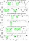 |
Fig. 32. Same as Fig. 31, but for six Gaia candidates in the LMC bar. The sources are Gaia DR3 4657899076482979328, 4658068847785992064, 4657993978084740992, 4657143097661657728, 4657909281189517056, 4657914336358760448. |
The second feature observed in Fig. 30 is an over-density of new Gaia candidates (with respect to OGLE4) at the location of the red clump at G ≃ 19 mag and GBP − GRP > 0.6 mag (upper-left panel) compared to the distribution of the cross-match sample (upper-middle panel). This could be either due to the lack of their detection in the OGLE survey, to variability of non-astrophysical origin, or to variability type misclassification. Investigation of the subsample of red-clump candidates defined with GBP − GRP > 0.7 mag, G > 18.7 mag, and G < 19.3 mag (2224 candidates) reveals that 59% of them belong to samples 2G-X, 2G-Y, or 2GE-Z, for which the binary nature requires confirmation. Furthermore, the global ranking of the subsample, and of the new LMC Gaia candidates in general, is low (see below), indicating large residuals. Yet, 5% of the subsample (112 sources) are detected as variables in the literature, the majority as eclipsing binaries by Kim et al. (2014). Additionally, a dozen of them are reported as RR Lyrae variables in the literature, including by the OGLE team. The classification of these faint candidates can be non-trivial due to potential light-curve geometry degeneracy within the photometric uncertainties between several variability types, such as sinusoidal-like type c RR Lyrae variables, ellipsoidal variables, and W UMa eclipsing binaries (the median G uncertainty at 18 mag is ∼0.024 mag). We also note that the Spearman correlation ripd, G of these new Gaia candidates in the LMC red clump shown in the bottom panel of Fig. 29 does not show any specific feature that would point to a non-astrophysical origin of the signal. The determination of the true nature of these LMC red clump candidates therefore requires further investigation.
The situation of the new Gaia candidates in the Galactic Bulge with respect to OGLE4 is very similar to the situation described above for the LMC, with the additional observation that the sky density is much higher in the Galactic Bulge than in the LMC, and the sources are much redder due to heavy extinction. As a result, C reaches very large values, above three, as shown in Fig. 33. This is particularly true for the new Gaia candidates with no OGLE4 cross-match (bottom panel in the figure) as compared to the sample with an OGLE4 cross-match (top panel). Among these new Gaia candidates compared to OGLE4, only very few have a detection as an eclipsing binary in other surveys. Their magnitude and global ranking distributions are shown in blue in the bottom panels of Figs. 27 and 28, respectively (note the 100× amplification factor compared to the distributions of the other samples). The higher level of sky crowdedness towards the Galactic Bulge may explain the larger fraction of new Gaia candidates in that region of the sky (65% compared to 53% towards the LMC; see Table 8). This fraction is still 35% in a sample limited to global ranking>0.5 towards the Galactic Bulge.
 |
Fig. 33. BP+RP flux excess factor versus colour of the Gaia eclipsing binaries in the sky area towards the Galactic Bulge shown in Fig. 25. Top panel: Gaia candidates with OGLE4 cross-matches. Bottom panel: Gaia candidates with no OGLE4 cross-match. The axes ranges have been truncated for greater visibility. |
In summary, more than half of the Gaia eclipsing binaries are new discoveries, the percentage being larger in crowded regions than in less dense regions of the sky. These new sources generally have low global rankings and large BP+RP flux excess factors, requiring that caution be exercised when using their GBP and GRP magnitudes. However, they show genuine G light curves of eclipsing binaries in many cases.
5. Illustrative samples
Samples of the Gaia DR3 eclipsing-binary candidates towards the LMC and the Galactic Bulge are briefly discussed in Sects. 4.2 and 4.3. In this section, we further illustrate the catalogue, first with the sample of candidates with good parallaxes (Sect. 5.1), and then by investigating the shortage of short-period eclipsing binaries in the Magellanic Clouds (Sect. 5.2).
5.1. Samples with good parallaxes
We consider positive relative parallax uncertainties better than 15% (409 437 sources) and restrict our analysis to sources with good BP+RP flux excess factors to exclude clearly erroneous GBP − GRP colours in colour–magnitude diagrams. We use for this the corrected BP+RP flux excess factor C* proposed by Riello et al. (2021), using the GBP and GRP median values in their Eq. (6). The distribution of this quantity for the sample with good parallaxes is shown in Fig. 34. We limit our sample to C* < 0.5. This removes 2% of the initial sample, leaving 400 996 sources. The resulting parallax distribution versus G magnitude is shown in Fig. 35. Most sources are brighter than ∼18 mag. Sources fainter than this value lie within 2 kpc of the Sun.
 |
Fig. 34. Corrected BP+RP flux excess factor versus colour of Gaia DR3 eclipsing binaries with positive parallax uncertainties better than 15%. Median values of GBP, GRP, and G are used in all quantities. The axis ranges have been truncated for greater visibility. |
 |
Fig. 35. Parallax in milliarcseconds versus median(G) of Gaia DR3 eclipsing binaries with positive parallax uncertainties better than 15% and corrected BP+RP flux excess factor smaller than 0.5. |
The absolute MG magnitude versus GBP − GRP colour diagram, hereafter referred to as the observational Hertzsprung-Russell (HR) diagram, is shown in Fig. 36. In the top panel, we show for reference the distribution of a sample of ten million sources extracted randomly from Gaia DR3 under the conditions of positive relative parallax uncertainty better than 5%, with at least 135 CCD measurements in G (field phot_g_n_obs in the Gaia archive) and at least 15 measurements in GBP and GRP (phot_rp_n_obs and phot_bp_n_obs, respectively), and with no multiple source detection (ipd_frac_multi_peak = 0). The distribution of the eclipsing binaries with good parallaxes is shown in the second panel. For comparison, contour lines of the distribution of the sample of ten million stars are added in grey. The sample of eclipsing binaries is seen to have a lower envelope of the main sequence shifted by ∼0.75 mag to the bright side compared to that of the sample of ten million stars (a convincing representation is shown in Fig. C.8), consistent with the magnitude shift expected for binary systems containing two main sequence stars of similar luminosities.
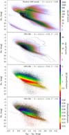 |
Fig. 36. Observational HR diagrams of Gaia DR3 stars with good parallaxes. Top panel: density map of a random sample of ten million stars with parallax uncertainties better than 5% and additional conditions on the number of measurements and source image quality (see text). The yellow lines are evolution tracks of, from bottom to top, 0.8, 1, 1.5, and 2 M⊙ solar-metallicity stellar models from Ekström et al. (2012). Second panel: density map of Gaia eclipsing-binary candidates with parallax uncertainties better than 15% and corrected BP+RP flux excess factors less than 0.5. Contour lines (logarithmic scale) of the sample shown in the top panel are drawn in grey. Third panel: same as second panel, but colour-coded with the median value of the orbital period in each bin. Bottom panel: same as second panel, but colour-coded with the median value of the global ranking in each bin. Median values of the GBP, GRP, and G cleaned time series are used in all panels except in the top one, where mean values are used due to the unavailability of median values for all sources in Gaia DR3. The colours in the figures are coded according to the colour scales to the right of each panel. The ranges of the axes and colour scales are truncated for greater visibility. |
Almost half of the eclipsing-binary candidates in this good parallax sample have an ellipsoidal component in their light-curve model, with 18% of the sample belonging to group 2GE-A and 22% to 2GE-B). An additional 24% are tight systems with the light curves described by two wide Gaussians (group 2G-B), and 10% belong to group 2G-A.
The orbital period distribution across the observational HR diagram is shown in the third panel from the top of Fig. 36, with the per-bin median period colour coded. The period is seen to be well correlated, on average, with the stellar radius, as expected for tight systems. However, this is not observed for intrinsically faint main sequence candidates with absolute MG ≳ 7 mag, or for candidates below the main sequence where cataclysmic variables are found. The global rankings of these faint candidates are generally also very low, as can be seen from the bottom panel of Fig. 36. The observational HR diagram displays a much tighter period–stellar radius correlation over the full magnitude range if we restrict the sample to candidates with high global rankings. This is illustrated in Fig. 37 with the sample of good parallaxes restricted to sources with a global ranking higher than 0.6, to which all 24 081 tight binaries from Sample 2G-C are also added5. More than half of this new sample of 144 994 sources have an ellipsoidal component (among which 21% in Sample 2GE-A and 38% in Sample 2GE-B), and 15% are in Sample 2G-B. The period distributions in the two samples, namely the full sample with good parallaxes and the sample restricted to high global rankings, are very similar, but systems with a strong ellipsoidal component (2GE-B) become predominant at short periods in the sample restricted to high global rankings, as shown in Fig. 38.
 |
Fig. 37. Same as third panel of Fig. 36, but for the subset with global rankings higher then 0.6 or belonging to the group 2G-C. |
 |
Fig. 38. Period distributions of the good parallax sample. The filled grey histogram represents the full distribution, while the orange, blue, magenta, red, and green histograms represent the 2G-A, 2G-B, 2G-C, 2GE-A, and 2GE-B subsamples, respectively. Top panel: all candidates in the good parallax sample with C* < 0.5. Bottom panel: same as top panel, but restricted to candidates with global rankings larger than 0.6 except for group 2G-C. |
Bright candidates without detected ellipsoidal variability. About ten percent of the sample with good parallaxes have two Gaussians in their light curve and no detected ellipsoidal variability (group 2G-A), pointing to detached systems (and some semi-detached ones; see Sect. 3.1). As expected, they have, on average, longer periods than the tighter systems (see Fig. 38). A key question concerns the circularisation of these systems at short periods. While we do not model the binary systems, and hence do not know their eccentricity, an eccentricity proxy eproxy can be derived from the relative eclipse locations and durations provided by the two-Gaussian model. The relevant equations are provided in Appendix B, where we show that most candidates in groups with potential tidal interactions (groups 2G-B, 2G-C, 2GE-A and 2GE-B) have eccentricity proxies compatible with circular systems, while large eccentricity proxies are found in Sample 2G-A of systems without detected tidal interaction. However, the analysis also reveals the unexpected presence of short-period systems with large eccentricity proxies (top panel of Fig. B.1), while these systems are expected to have been circularised.
In order to check the status of these short-period systems with large eccentricity proxies, we focus on the subset of bright candidates with G < 12 mag. There are 401 such candidates in the good parallax sample with large global rankings defined above. Their P–eproxy diagram is shown in Fig. 39. The eccentricity limit above which all systems at a given period are expected to be circular is shown by the dashed blue line, following Eq. (4.4) of Mazeh (2008) with E = 0.98, A = 3.25, B = 6.3, and C = 0.23. The figure shows 48 systems that are unexpectedly above this limit; we refer to these as outlier sources. The uncertainty on their eccentricity proxy, a quantity that can be computed from the parameter uncertainties of the two-Gaussian model (see Eq. (B.4)), does not resolve the issue. If we take the 1σ lower values of the eccentricity proxies considering their ε(eproxy) uncertainties, 27 candidates remain above the limit (the 1σ downward corrections are shown as vertical grey line segments in Fig. 39), and 14 still have a 2σ downward correction. The depth of the secondary eclipse is colour-coded in Fig. 39, red corresponding to shallow dips and blue to deep dips. Most of the outliers are seen to have very shallow secondary eclipses, namely less than ten milli-magnitudes in depth (red markers in the figure). The figure also encodes the secondary over primary depths ratios, with the size of the markers proportional to this ratio such that smaller circles correspond to smaller depth ratios. The large majority of the outliers are seen to have a secondary eclipse that is much shallower than the primary eclipse (small marker size). These features suggest careful verification of the reliability of the secondary eclipse is required.
 |
Fig. 39. Eccentricity proxy versus orbital period of Sample 2G-A eclipsing binaries (well-detached and without ellipsoidal component) that are brighter than 12 mag in G and that have parallax uncertainties better than 15%, a corrected BP+RP flux excess factor lower than 0.5, and global rankings higher than 0.6. The colour of each marker is related to the depth of the secondary eclipse (in G magnitude) according to the colour-scale to the right of the figure, with ratios larger than 0.45 rendered in black. The size of each marker is proportional to the secondary over primary depth ratio. The vertical line segments indicate the 1σ uncertainty of the eccentricity proxy. For clarity, this error has only been drawn on the small eccentricity side. The blue dashed line is Eq. (4.4) from Mazeh (2008) with E = 0.98, A = 3.25, B = 6.3, and C = 0.23. The five sources above this line that are highlighted with open diamonds have their light curves displayed in Fig. 41. |
A comparison of the Gaia periods with literature periods, when available, provides additional insight. The top panel of Fig. 40 shows this comparison for candidates that have acceptable eccentricity proxies, that is, below the expected upper limit. A very good match between PGaia and Plit is seen for a large majority of the sources, with most of them having a 1:1 ratio and some a 1:2 ratio (PGaia ≃ 2 Plit). In contrast, only very few outlier sources have PGaia ≃ Plit, as shown in the bottom panel of Fig. 40, but the majority of them still have a Gaia period ‘compatible’ with the literature period within a factor of two, with PGaia ≃ 0.5 Plit. This suggests that the Gaia pipeline considered the two distinct eclipses as one unique eclipse, and detected a (usually very shallow) artefact in the folded light curve to represent an imaginary secondary eclipse. A typical example of such a case is shown in the top panel of Fig. 41, where the secondary has a very shallow secondary dip identified at phase around 0.1, barely visible in the figure. If we increase the Gaia period of the outlier sources by a factor of two, the majority of them become compatible with the expected maximum eccentricity given their period in Fig. 39. We note that in that case, the eccentricity proxy would also take another value as the two-Gaussian model will be different.
 |
Fig. 40. Same as Fig. 39, but for non-Gaia literature period versus Gaia period for those sources that have a period published in the literature. The dashed line is PLit = PGaia, and the dotted lines are the relations PLit = 2 PGaia and PLit = 0.5 PGaia. Top panel: sources that have eccentricity proxies smaller than the eccentricity limit shown in Fig. 39. Bottom panel: sources with eccentricity proxies larger than this limit. |
The above analyses suggest that a quick way to clean the P–eproxy diagram in Fig. 39 is to remove all small red points. If we do this, a few outlier sources will still remain, which have significant secondary eclipse depths both in terms of absolute depth (non-red colour) and of secondary over primary depth ratio (large marker sizes). We investigate the four systems with the shortest periods below. These are, in increasing order of orbital period, Gaia DR3 4524651705941314432 (0.2411507 d), 5712304991851559040 (0.2450746 d), 2589992273084612480 (0.2818606 d), and 4455992049496820992 (0.3682685 d). They are identified with open diamonds in Fig. 39, and their G, GBP, and GRP light curves are shown in Fig. 41. All two-Gaussian models to the G light curves (dashed lines in the figure) appear acceptable. However, a closer look reveals some features that lead us to question the periods extracted from the G light curves, which have only a small number of measurements in the eclipses. Investigation of the GBP and GRP light curves, which were not used in the DR3 processing of eclipsing binaries, suggest that the periods derived from the G light curves may be incorrect, at least for the second and third sources. Therefore, the periods of these outlier sources should be double checked.
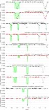 |
Fig. 41. Same as Fig. 4, but for five bright candidates with eccentricity proxies larger than the expected limit shown in Fig. 40. From top to bottom: Gaia DR3 2888711169825554688, 4524651705941314432, 5712304991851559040, 2589992273084612480 and 4455992049496820992. |
Two of these four outliers are identified in the ASAS-SN survey as eclipsing binaries (Jayasinghe et al. 2019), but with different periods from the Gaia period. Gaia DR3 4524651705941314432 is mentioned with a period of 3.3972697 d (ASASSN-V J075432.26-211826.4), and Gaia DR3 5712304991851559040 with a period of 5.9965616 d (ASASSN-V J184156.16+192755.8). Their Plit versus PGaia values are highlighted by the diamonds in the bottom panel of Fig. 40. The Gaia DR3 4524651705941314432 light curve is compatible with the ASAS-SN period (see Fig. C.9 which displays the Gaia light curve folded with the ASAS-SN period). However, this period was not selected by the automated Gaia pipeline because of the scarcity of points that would result in the secondary eclipse. Regarding Gaia DR3 5712304991851559040, the period proposed by ASAS-SN is not compatible with the Gaia light curve. The ASAS-SN period is actually not compatible with the ASAS-SN light curve6 either. However, twice this period (11.9931232 d) would be compatible with both ASAS-SN and Gaia light curves. Nevertheless, here too, the scarcity of Gaia measurements that would result in the secondary eclipse prevented the Gaia pipeline from chosing this period.
In summary, Gaia results of eclipsing binaries are generally very good given the available Gaia time series. However, further investigations must be performed for specific cases. This is especially true for well-detached eclipsing binaries with long periods, for which an incorrect (very) short period may instead be chosen as the best solution by the DR3 pipeline.
5.2. Short-period binaries in the Magellanic Clouds
The period distributions of eclipsing binaries in the Magellanic Clouds are shown in Fig. 42. Here, we have excluded candidates from groups 2G-D, 2G-X, 2G-Y, and 2GE-Z, for which the periods are less reliable, and include only candidates with global rankings above a certain limit as mentioned in the caption of the figure in order to limit the impact of aliases (see Sects. 3.3 and 3.4). The distributions of both the LMC (blue filled histogram in the figure) and SMC (red filled histogram) peak at values above 1 day (∼1.7 and ∼1.3 d, respectively), in contrast to the distribution of candidates in the Galaxy, which peaks at ∼0.33 day (grey histogram). This shortage of short-period (less than about 1 day) eclipsing binaries in the Magellanic Clouds has already been reported by the OGLE survey team (Pawlak et al. 2016).
 |
Fig. 42. Period distributions of eclipsing-binary candidates with global rankings higher than 0.5 (>0.45 for Sample 2G-B). Samples 2G-D, 2G-X, 2G-Y, and 2GE-Z are excluded. The distributions of candidates satisfying these conditions towards the LMC and SMC, with sky position, proper motion, and parallax criteria taken from Mowlavi et al. (2019), are shown in blue and red, respectively. The distribution of the remaining sources satisfying these conditions is shown with the filled grey histogram. The distributions are normalised to their maximum values. |
The Gaia data allow us to confirm the origin of this observed shortage. The absolute magnitudes of the tight systems (see Table 3) with relative parallax uncertainties better than 10% and global ranking above 0.5 (above 0.45 for candidates in Sample 2G-B) are shown versus their orbital period in Fig. 43 (in grey). A clear correlation is visible of decreasing period with decreasing brightness, resulting in a lack of systems with periods shorter than 0.5 days at magnitudes brighter than MG ≃ 1.5 mag. This limit translates to an apparent magnitude G ≃ 20 at the distance of the LMC, considering a distance modulus of 18.476 mag (Pietrzyński et al. 2019), explaining the lack of short-period systems in the LMC, as hypothesised in Pawlak et al. (2016). The distribution of the Gaia tight systems in the LMC is shown in red in Fig. 43. The same conclusion is reached with the sample of wide systems in groups 2G-A and 2GE-A. Despite a less pronounced correlation between MG and P, a lack of these wide system with periods shorter than about 1 day is observed at absolute magnitudes brighter than MG ≃ 1.5 mag. For illustrative purposes, the observational HR diagram of the Galactic and LMC tight systems discussed above is shown in Fig. 44.
 |
Fig. 43. Absolute G magnitude versus orbital period for tight system candidates (samples 2G-B, 2G-C, 2GE-B, 1GE and 0GE) with global ranking higher than 0.5 (> 0.45 for Sample 2G-B). Sources with relative parallax uncertainties better than 10% in the Galaxy are shown in grey and sources towards the LMC (same selection criteria as in Fig. 42) are shown in red. A distance modulus of 18.476 mag is adopted from Pietrzyński et al. (2019) for the LMC. |
 |
Fig. 44. Observational HR diagram of Gaia DR3 for the tight candidates shown in Fig. 43, displayed as a density map for Galactic sources (colour-coded according to the colour scale to the right of the figure) and as red circles for candidates towards the LMC (same selection criteria as in Fig. 42). The contour lines (logarithmic scale) of the random sample of ten million stars shown in the top panel of Fig. 36 are drawn in black. |
6. Summary and conclusions
This paper presents the first Gaia catalogue of eclipsing binaries made available in June 2022 within Gaia DR3. It contains more than two million candidates, which are filtered from a larger set of eclipsing-binary candidates identified by the general classification pipeline of the variability processing modules within the Gaia DPAC (Rimoldini et al. 2023). The orbital periods are determined based on the cleaned G light curves. A two-Gaussian model is used to characterise the morphology of their light curves –which contains up to two Gaussian functions and one sine function– and a global ranking is provided that quantifies the quality of the model fit to the G light curves. The model adequately identifies the eclipses and ellipsoidal variability when they are clearly detectable in the light curves, and several groups of eclipsing binaries, from wide to tight systems, are identified in Sect. 3.1 based on the model parameters. However, the two-Gaussian model can contain components that are not relevant to describing real eclipses or ellipsoidal variability, though they reliably describe the geometry of the light curves. The GBP and GRP light curves were not considered in the processing of the eclipsing binaries in DR3.
About 600 000 of the Gaia candidates have a cross-match in the literature, of which 88% are also identified as eclipsing binaries in the literature. The Gaia and literature periods are similar for 86% of the sources identified as eclipsing binaries in both Gaia and the literature. This number increases to 93% when also considering period ratios of two. The overall completeness of the catalogue is estimated to lie between 25% and 50% –depending on the sky region– based on a comparison with OGLE4 catalogues of eclipsing binaries towards the Magellanic Clouds and the Galactic Bulge. More than half of the catalogue consists of new candidates, with larger percentages of new candidates in dense regions of the sky. We estimate that overall perhaps 6% of our candidates could be affected by scan-angle-dependent signals in their photometry (Sect. 3.5), meaning that their reported period and model is likely wrong even though a subset of them will be of eclipsing-binary origin.
Illustrative samples with good parallaxes –with the majority being tight systems– confirm that their properties, such as distribution in the observational HR diagram and periods, are as expected overall. The analysis of the period–eccentricity diagram for a subset of detached systems, on the other hand, highlights the challenges in dealing with these systems, and illustrates how the catalogue can be used. Finally, we show how the sample of Galactic short-period (less than 1 day) systems with good parallaxes confirms the observational origin of the lack of short-period systems in the Magellanic Cloud.
This release represents the largest catalogue of eclipsing-binary candidates available so far in the literature. Looking to the future, the next Gaia Data Release 4 (DR4) will provide an even larger catalogue of candidates, with improved characterisation due not only to the larger time baseline and increased number of measurements (DR4 will be based on 66 months of data instead of the 34 months in DR3), but also to further improvements in our processing pipeline by, for example, taking into account GBP and GRP time series.
305 binaries on Aug. 30, 2022, see https://www.astro.keele.ac.uk/jkt/debcat
The GBP and GRP light curves of SW Cyg as well as of the other binaries mentioned in this section are displayed in Appendix C.
Most OGLE4 eclipsing binaries in the Magellanic Clouds are on the main sequence. In contrast, in the Galactic Bulge, they are red sources. This is reflected in their I, V, and G magnitudes shown in Fig. C.7.
Downloaded from the ASAS-SN database of light curves at https://asas-sn.osu.edu/variables
When the model includes an ellipsoidal (cosine) term, the Gaussian widths are, by construction, smaller than 0.4/5.6 = 0.0714 to avoid a degenerative competition between the wide Gaussian and the cosine functions (see Sect. 2.2 in the main body of the text).
Acknowledgments
We thank the referee for useful comments. Specific acknowledgements related to the Gaia data on which this work is based are given in Appendix D. This research has made use of the free Starlink Tables Infrastructure Library (STILTS and TOPCAT, Taylor 2006). This research has made use of NASA’s Astrophysics Data System Bibliographic Services.
References
- Alcock, C., Allsman, R. A., Alves, D., et al. 1997, ApJ, 486, 697 [NASA ADS] [CrossRef] [Google Scholar]
- Andersen, J. 1991, A&A Rev., 3, 91 [Google Scholar]
- Avvakumova, E. A., Malkov, O. Y., & Kniazev, A. Y. 2013, Astron. Nachr., 334, 860 [Google Scholar]
- Burke, E. W., Jr, Rolland, W. W., & Boy, W. R. 1970, JRASC, 64, 353 [NASA ADS] [Google Scholar]
- Chen, X., Wang, S., Deng, L., et al. 2020, ApJS, 249, 18 [NASA ADS] [CrossRef] [Google Scholar]
- Cumming, A., Marcy, G. W., & Butler, R. P. 1999, ApJ, 526, 890 [Google Scholar]
- Devor, J., Charbonneau, D., O’Donovan, F. T., Mandushev, G., & Torres, G. 2008, AJ, 135, 850 [Google Scholar]
- Drake, A. J., Djorgovski, S. G., Catelan, M., et al. 2017, MNRAS, 469, 3688 [NASA ADS] [CrossRef] [Google Scholar]
- Ekström, S., Georgy, C., Eggenberger, P., et al. 2012, A&A, 537, A146 [Google Scholar]
- ESA 1997, in The HIPPARCOS and TYCHO catalogues. Astrometric and photometric star catalogues derived from the ESA HIPPARCOS Space Astrometry Mission, ESA Spec. Publ., 1200 [Google Scholar]
- Eyer, L., Mowlavi, N., Evans, D. W., et al. 2017, ArXiv e-prints [arXiv:1702.03295] [Google Scholar]
- Eyer, L., Audard, M., Holl, B., et al. 2023, A&A, 674, A13 (Gaia DR3 SI) [NASA ADS] [CrossRef] [EDP Sciences] [Google Scholar]
- Feigelson, E. D., & Babu, G. J. 2012, Modern Statistical Methods for Astronomy (Cambridge University Press) [Google Scholar]
- Gaia Collaboration (Prusti, T., et al.) 2016, A&A, 595, A1 [NASA ADS] [CrossRef] [EDP Sciences] [Google Scholar]
- Gaia Collaboration (Brown, A. G. A., et al.) 2021, A&A, 649, A1 [NASA ADS] [CrossRef] [EDP Sciences] [Google Scholar]
- Gaia Collaboration (Arenou, F., et al.) 2023a, A&A, 674, A34 (Gaia DR3 SI) [CrossRef] [EDP Sciences] [Google Scholar]
- Gaia Collaboration (Vallenari, A., et al.) 2023b, A&A, 674, A1 (Gaia DR3 SI) [NASA ADS] [CrossRef] [EDP Sciences] [Google Scholar]
- Gavras, P., Rimoldini, L., Nienartowicz, K., et al. 2023, A&A, 674, A22 (Gaia DR3 SI) [NASA ADS] [CrossRef] [EDP Sciences] [Google Scholar]
- Heck, A., Manfroid, J., & Mersch, G. 1985, A&AS, 59, 63 [NASA ADS] [Google Scholar]
- Heinze, A. N., Tonry, J. L., Denneau, L., et al. 2018, AJ, 156, 241 [Google Scholar]
- Holl, B., Fabricius, C., Portell, J., et al. 2023, A&A, 674, A25 (Gaia DR3 SI) [NASA ADS] [CrossRef] [EDP Sciences] [Google Scholar]
- Jayasinghe, T., Stanek, K. Z., Kochanek, C. S., et al. 2019, MNRAS, 486, 1907 [NASA ADS] [Google Scholar]
- Jurkevich, I. 1971, Ap&SS, 13, 154 [NASA ADS] [CrossRef] [Google Scholar]
- Kim, D.-W., Protopapas, P., Bailer-Jones, C. A. L., et al. 2014, A&A, 566, A43 [CrossRef] [EDP Sciences] [Google Scholar]
- Kirk, B., Conroy, K., Prša, A., et al. 2016, AJ, 151, 68 [Google Scholar]
- Lafler, J., & Kinman, T. D. 1965, ApJS, 11, 216 [NASA ADS] [CrossRef] [Google Scholar]
- Malkov, O. Y. 2020, MNRAS, 491, 5489 [NASA ADS] [CrossRef] [Google Scholar]
- Mazeh, T. 2008, EAS Publ. Ser., 29, 1 [NASA ADS] [CrossRef] [EDP Sciences] [Google Scholar]
- Mowlavi, N., Lecoeur-Taïbi, I., Holl, B., et al. 2017, A&A, 606, A92 [NASA ADS] [CrossRef] [EDP Sciences] [Google Scholar]
- Mowlavi, N., Trabucchi, M., & Lebzelter, T. 2019, The Gaia Universe, 62 [Google Scholar]
- Paczyński, B., Szczygieł, D. M., Pilecki, B., & Pojmański, G. 2006, MNRAS, 368, 1311 [CrossRef] [Google Scholar]
- Palaversa, L., Ivezić, Ž., Eyer, L., et al. 2013, AJ, 146, 101 [CrossRef] [Google Scholar]
- Pawlak, M., Soszyński, I., Udalski, A., et al. 2016, Acta Astron., 66, 421 [Google Scholar]
- Pietrzyński, G., Graczyk, D., Gallenne, A., et al. 2019, Nature, 567, 200 [Google Scholar]
- Pigulski, A., Pojmański, G., Pilecki, B., & Szczygieł, D. M. 2009, Acta Astron., 59, 33 [NASA ADS] [Google Scholar]
- Pojmanski, G. 2002, Acta Astron., 52, 397 [NASA ADS] [Google Scholar]
- Prša, A., Kochoska, A., Conroy, K. E., et al. 2022, ApJS, 258, 16 [CrossRef] [Google Scholar]
- Renault, C., Aubourg, E., Bareyre, P., et al. 1998, A&A, 329, 522 [NASA ADS] [Google Scholar]
- Riello, M., De Angeli, F., Evans, D. W., et al. 2021, A&A, 649, A3 [NASA ADS] [CrossRef] [EDP Sciences] [Google Scholar]
- Rimoldini, L., Holl, B., Gavras, P., et al. 2023, A&A, 674, A14 (Gaia DR3 SI) [NASA ADS] [CrossRef] [EDP Sciences] [Google Scholar]
- Schwarzenberg-Czerny, A. 1997, Astron. Time Ser., 218, 183 [NASA ADS] [CrossRef] [Google Scholar]
- Sesar, B., Hernitschek, N., Mitrović, S., et al. 2017, AJ, 153, 204 [NASA ADS] [CrossRef] [Google Scholar]
- Soszyński, I., Pawlak, M., Pietrukowicz, P., et al. 2016, Acta Astron., 66, 405 [NASA ADS] [Google Scholar]
- Southworth, J. 2015, ASP Conf. Ser., 496, 164 [NASA ADS] [Google Scholar]
- Stellingwerf, R. F. 1978, ApJ, 224, 953 [Google Scholar]
- Taylor, M. B. 2006, ASP Conf. Ser., 351, 666 [Google Scholar]
- Udalski, A., Szymanski, M., Kaluzny, J., Kubiak, M., & Mateo, M. 1992, Acta Astron., 42, 253 [NASA ADS] [Google Scholar]
- Wall, J. V., & Jenkins, C. R. 2003, Practical Statistics for Astronomers, 3 (UK: Cambridge University Press) [CrossRef] [Google Scholar]
- Watson, C. L., Henden, A. A., & Price, A. 2006, Soc. Astron. Sci. Ann. Symp., 25, 47 [NASA ADS] [Google Scholar]
- Zechmeister, M., & Kürster, M. 2009, A&A, 496, 577 [CrossRef] [EDP Sciences] [Google Scholar]
Appendix A: Analysis of the two-Gaussian model parameters
This Appendix provides some insight into the two-Gaussian model properties of the Gaia DR3 catalogue of eclipsing-binary candidates. In Sects. A.1 and A.2, we discuss the cases of models including two Gaussians, which constitute the overwhelming majority of the catalogue (94% of the candidates; see Table 1 in the main body of the article). Models containing one Gaussian (4% of the catalogue) are then considered in Sects. A.3 and A.4. The remaining 2% of candidates, whose light curves are modelled with only an ellipsoidal component, are discussed in Sect. A.5. A summary is provided in Sect. A.6.
A.1. Models with only two Gaussians
Almost three quarters (73%) of the sources in the catalogue have their light curves modelled by two Gaussians and without an ellipsoidal component. These are identified in the Gaia table with model_type=TWOGAUSSIANS or num_model_parameters = 8.
The distributions of the phase widths σp and σs of their primary and secondary Gaussian functions, respectively, are shown in Fig. A.1 (top panel). The bulk of the sources lie along the diagonal line of equal Gaussian widths, where two distinct samples can be discerned. We define samples 2G-A and 2G-B as the ones at smaller and larger width, respectively. A third distinct sample is visible at σp ≳ 0.17, which we label Sample 2G-C. The exact definition of each sample is given in Table A.1, and their locations in the σp – σs plane are summarised in Fig. A.2. We briefly describe their properties in the following paragraphs.
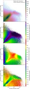 |
Fig. A.1. Secondary versus primary Gaussian widths for models without an ellipsoidal component. The widths are expressed in phase units. Top panel: Density map of the sample, colour-coded according to the colour-scale shown to the right of the panel. Second panel: Bin-median value of the phase separation of the two Gaussians, shifted between 0 and 0.5. Third panel: Bin-median value of secondary to primary Gaussian depths ratio. Bottom panel: Bin-median value of global ranking. The values are colour-coded according to the colour-scales to the right of each panel. The axes ranges have been restricted for better visibility. |
 |
Fig. A.2. Distribution in the primary versus secondary Gaussian width plane of the samples defined in Table A.1 for the models without an ellipsoidal component. |
Sample definition.
Sample 2G-A.
The first sample identified along the diagonal line of equal Gaussian widths at phase widths smaller than ∼0.06 (blue region in Fig. A.2) contains well detached eclipsing binaries. It can also contain semi-detached systems if the star that fills its Roche Lobe is much fainter than the primary star such that the ellipsoidal variability induced by the pear-shaped faint companion remains undetected in the light curve. In this case, the secondary eclipse is expected to be much shallower than the primary eclipse. The two Gaussians in Sample 2G-A are separated by 0.5 in phase in the majority of cases, as shown in the second panel from top in Fig. A.1, suggesting circular orbits for the majority of them. Two example light curves7 are shown in Fig. A.3, one with a circular orbit and one with an eccentric orbit.
 |
Fig. A.3. Example G light curves (top panels in each set) and GBP and GRP light curves (bottom panels in each set) of sources in Sample 2G-A modelled with only two Gaussians. The GBP and GRP magnitudes are shifted by a value equal to their median magnitudes, the values of which are given in the panel. The two-Gaussian model obtained from the G light curve is superposed as a dotted line in both panels of each set. The green areas indicate the derived eclipse durations. The top set is for the circular candidate Gaia DR3 5632871775033302656 and the bottom set is for the eccentric candidate Gaia DR3 2059784985669541760. |
The depth ratio between the two eclipses takes all values between (close-to) zero and one (thin blue histogram in the top panel of Fig. 6 in the main body of the text), suggesting, for close-to-circular systems, a wide range of luminosity ratios between the two binary stars. The median value of this ratio is about 0.6 in all bins in the σp – σs diagram where σp ≃ σs, as seen in the third panel of Fig. A.1. However, the per-bin median depth ratio drops quickly when moving away from the equal-width area, with ratios reaching below 0.3 at the edges of the 2G-A region. This may indicate the presence of sources for which the two Gaussians are not catching the real eclipse dips. Two-Gaussian models that realistically describe the eclipse properties of well-detached eclipsing binaries are expected to have similar Gaussian widths.
Detection of spurious eclipses by the automated algorithm is unavoidable. An example of such a case is shown in Fig. A.4 (top example), where a spurious shallow dip detected close to the primary eclipse is identified as the secondary eclipse, which is probably due to the lack of measurements at a phase distant by 0.5 from the primary, or due to a period that is too small by a factor of two. We note that the primary eclipse still appears to be correct in that example. A visual check of a random set of 100 sources in Sample 2G-A leads to an estimated 5%-10% sources that could have spurious secondary-eclipse identifications.
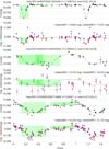 |
Fig. A.4. Same as Fig. A.3, but illustrating cases of incorrect model identifications. From top to bottom sets: Spurious secondary eclipse identification in Sample 2G-A (Gaia DR3 264837033617656448), incorrect period estimate in Sample 2G-B (Gaia DR3 4045605519248336256), spurious ellipsoidal variable in Sample 2G-C (Gaia DR3 2195008530582714880). |
Finally, we must caution that an eclipse may lack sufficient phase coverage to properly constrain its depth. An example of such a case is shown in Fig. A.5. The Gaussian depths and derived eclipse depths are consequently much larger than the magnitude range of the observations, as expected from the lack of observations in the faint parts of the eclipse. Additional observations are needed to confirm the true eclipse depth of these cases. Figure A.6 (top panel) reveals that this mainly occurs for eclipse durations between ∼0.07 and ∼0.17 days. These durations correspond to the time intervals between successive passages in the Gaia FOVs, which are 1.775 hours from FOV1 to FOV2 and 4.225 hours from FOV2 to FOV1 given the six-hour rotation period of the spacecraft and the 106.5 degree basic angle between the two FOVs. For eclipse durations in this time interval, observations of a particular source may be lacking in the core of its eclipse depending on the observation time distribution over the 34 months covered in DR3. Let us consider such a source where only very few observations fall in its eclipse time window during these 34 months. For durations longer than 4.2 h, the probability of having measurements inside the eclipse is large, as the source will be observed during a minimum of two successive FOV passages. For durations shorter than 4.2 h (but larger than 1.8 h), the probability of having sufficient observations in the middle of the eclipse decreases with decreasing eclipse duration. If measurements are still available at the edge of the eclipse, the eclipse will be caught by the pipeline, but with rather unconstrained eclipse depth. For durations shorter than 1.8 h, the probability of having observations only at the edges of the eclipse decreases considerably as this duration is shorter than the shortest time interval between two successive FOVs. These aspects explain the excess of sources with (excessively) large primary eclipse depths in Fig. A.6 for eclipse durations between ∼0.07 and ∼0.17 days.
 |
Fig. A.5. Same as Fig. A.3, but for a case (Gaia DR3 5684917462874690560) with an insufficient coverage of the primary eclipse that leads to the poor constraint of its depth. |
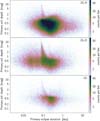 |
Fig. A.6. Density map of the primary eclipse depth versus duration (in days) for the samples 2G-A (top panel), 2G-D (middle panel), and 1G (bottom panel). The primary eclipse duration is taken equal to wecl, 1 Porb. The larger occurrence of eclipse depths larger than about 1 mag for eclipse durations between ∼0.07 and ∼0.17 days is linked to the equivalent time intervals between successive observations in the two Gaia FOVs (see text, Sect. A.1). The axis ranges have been limited for improved visibility. |
Sample 2G-B.
The second sample identified along the line of equal Gaussian widths in the top panel of Fig. A.1 lies at phase widths between 0.06 and 0.15. This is the most populated region in the diagram. Their larger Gaussian widths lead to the absence of flat inter-eclipse phases. These are tighter binaries than candidates in Sample 2G-A. The phase separation between the two eclipses is close to 0.5 (see second panel from top of Fig. A.1), as expected for these types of eclipsing binaries. The distribution of the eclipse depth ratio (green thick histogram in the top panel of Fig. 6) peaks at a value of 1 with a tail extending down to below 0.4. Example light curves are shown in Fig. A.7.
 |
Fig. A.7. Same as Fig. A.3, but for two sources in Sample 2G-B of light curves modelled with only two Gaussians. The top set is for EW-type eclipsing-binary candidate Gaia DR3 5256648720295981184 and the bottom set is for EB-type eclipsing-binary candidate Gaia DR3 1807942504467443456. |
In this sample 2G-B, spurious cases can happen when a potentially erroneous period is obtained. An example of such a case is shown in the second source from the top in Fig. A.4. Visual inspection of a random set of 100 sources in Sample 2G-B reveals only one such case, suggesting a very low fraction of spurious cases on the order of 1%.
Sample 2G-C.
A subset of the sources shown in the top panel of Fig. A.1 forms a distinct group —at primary Gaussian widths larger than ∼0.17— from the majority of the sources that lie along the diagonal line of equal Gaussian widths. We define this subset as Sample 2G-C; it represents less than 2% of the TWOGAUSSIANS models. The light curves of these sources are modelled with two wide and deep overlapping Gaussians. When the Gaussians have similar depths and widths, which is the case at σp ≃ 0.2, the light-curve shape is close to sinusoidal. An example is shown in Fig. A.8 (top case). For σp values above 0.2, σs decreases with increasing σp. These sources are ellipsoidal binaries with light-curve modulations. An example is given by the second case in Fig. A.8. The change of light-curve shape with increasing σp of these Sample 2G-C sources is illustrated in the third panel of Fig. A.1, where the per-bin median depth ratio decreases from above 0.9 at σp ≃ 0.2 (red colours) to about 0.6 at σp ≃ 0.35 (green colours).
 |
Fig. A.8. Same as Fig. A.3, but for two ellipsoidal variable candidates from Sample 2G-C of light curves modelled with only two Gaussians. The top set is for a typical ellipsoidal variable (Gaia DR3 1872983530689181312) and the bottom panel for an ellipsoidal variable with light amplitude modulation (Gaia DR3 1980590328522237824). |
The phase separation between the locations of the two Gaussians is expected to be ∼0.5 for these tight systems. This is indeed confirmed for the majority of the sources in the sample (see second panel from top in Fig. A.1), with 90% of them having a deviation from a 0.5 separation of less than 0.015 in phase. The ones with larger deviations are spurious cases. An example light curve of such an apparently spurious case is shown by the third case in Fig. A.4.
The global ranking of the candidates in Sample 2G-C is generally lower than that of the candidates of samples 2G-A and 2G-B, with only very few cases above 0.6. This is shown in the top panel of Fig. A.9. Nevertheless, the light curves are very good in the majority of cases.
Finally, we must mention the value of derived_primary_ecl_depth (and derived_secondary_ecl_depth) reported in the catalogue for these 2G-C binaries. This value represents the depth of the faintest point of the primary dip in the modelled light curve. For most of the candidates in the catalogue, the value of derived_primary_ecl_depth is similar to the depth of the deepest Gaussian. When there is a significant overlap between the two Gaussian components, as is the case for candidates in Sample 2G-C, a significant difference exists between the depths of the Gaussians and the derived depths in the modelled light curve. This is illustrated in the top panel of Fig. A.10, which compares these two values for the primary Gaussian of models containing only two Gaussians. Sample 2G-C is identified as the distinctive subsample below (and almost parallel to) the diagonal line, with primary Gaussian depths (on the abscissa) that are between two and ten times larger than the actual depth in their light curves (on the ordinate).
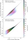 |
Fig. A.10. Density map of the depth of the primary eclipse versus the depth of the deepest Gaussian. The sample of sources whose light curves are modelled with two Gaussians and without an ellipsoidal component is shown in the top panel, while those with two Gaussians and a cosine function are shown in the bottom panel. The density in the maps is colour coded according to the colour scales shown to the right of each panel. The axes ranges have been restricted for better visibility. |
Sample 2G-D.
The remaining areas in Fig. A.1 (top panel) other than the ones defined by samples 2G-A, 2G-B, and 2G-C contain a variety of light-curve geometries. Among them, the ones with narrow primary and much wider secondary Gaussians stand out, with secondary Gaussian depths that are much smaller, in general, than the primary Gaussian depths, as seen in the third panel of Fig. A.1. We therefore define Sample 2G-D with σp ≲ 0.02 and σs ≳ 3 σp. The histogram of their depth ratio is shown by the cyan dotted histogram in Fig. 6 (bottom panel). Most of them have depth ratios lower than 0.2. This sample contains about 5% of the full catalogue.
While their primary Gaussians correctly identify the presence of a detached eclipse in most cases, caution must be taken as to the reality of the second Gaussian identification. The automated algorithm can indeed fail to detect a narrow secondary eclipse in the case of inadequate phase coverage and/or an overly shallow secondary, and instead pick up a wide and shallow feature in the light-curve geometry for the secondary eclipse. This can also result from an incorrect orbital period, for example if the true period is twice the determined period. An example of such a light curve is shown in the top panel of Fig. A.11, where the failure to detect a secondary eclipse may be due to either a lack of observations in the phase range distant by 0.5 from the primary eclipse (if circular orbit), or to a period determination (3.07 d) that is half the true value. Instead, a physically improbable wide and shallow secondary is picked up by the automated pipeline at a phase 0.3 apart from the primary. The GBP and GRP light curves confirm these conclusions drawn from the G light curve. The second example in Fig. A.11 illustrates a case where the GBP and GRP light curves would not be useful were they to be considered in the analysis, as they lack reliable observations due to the source being faint and lying in a dense region on the sky close to the Galactic bulge.
 |
Fig. A.11. Same as Fig. A.3, but for two candidates in Sample 2G-D of light curves modelled with only two Gaussians. The top set shows a case with a convincing primary eclipse detection while the secondary eclipse is spurious (Gaia DR3 2056622657089571968). The bottom set shows a seemingly good case from the G light curve (Gaia DR3 4077271415493214080). |
It must also be mentioned that a fraction of sources in this 2G-D sample lack sufficient observations to properly constrain their eclipse depth. This was already noted for Sample 2G-A at eclipse durations between 0.07 and 1.5 days (top panel of Fig. A.6). The same is true in this sample 2G-D, as clearly seen in the middle panel of Fig. A.6, affecting an even larger fraction of sources in this sample than in Sample 2G-A due to the shorter eclipse durations of the candidates in Sample 2G-D. Sources in this sample merit additional investigation using Gaia data themselves and/or complementary observations.
Samples 2G-X and 2G-Y.
The two remaining areas in Fig. A.1, namely the areas above and below the area of equal Gaussian widths (which respectively define samples 2G-X and 2G-Y), contain sources with various light-curve model geometries. Their Gaussian depth ratios span all values from almost 0 up to 1 (yellow and pink histograms in the bottom panel of Fig. 6, respectively). The phase separation between the two Gaussians also has a wider distribution than those of Samples 2G-A to C, with median values between 0.4 and 0.45 (greenish regions in the second panel of Fig. A.1). Both these features suggest that a careful investigation of the light curves is required, as the two-Gaussian model components may be insufficient to account for the physics of the binary system that determines its light variability. This is also suggested from their generally low global rankings shown in the bottom panel of Fig. A.1, with median per-bin values below 0.48 for a majority of them (yellowish and reddish colours in the panel). The histograms of their global rankings shown in the bottom panel of Fig. A.9 confirm this. Restricting the samples to sources with global rankings greater than 0.52 removes much of the sources in samples 2G-X and 2G-Y, as shown in Fig. A.12 (to be compared with the top panel of Fig. A.1). The total number of sources in each of these two samples amounts to about 10% of the full catalogue.
 |
Fig. A.12. Same as the top panel of Fig. A.1, but for the subset of sources with global rankings higher than 0.52. The colour scale is kept identical to that of the top panel of Fig. A.1 to allow direct comparison. |
A.2. Models with two Gaussians and an ellipsoidal component
About one-quarter (23%) of the sources in the catalogue have their G light curves modelled with two Gaussians and an additional ellipsoidal (cosine) component. The two Gaussians have similar widths 8 (see Fig. A.13), reminiscent of Sample 2G-A of wide binaries identified in Sect. A.1. However, contrary to Sample 2G-A, Sample 2GE-A candidates are all tight systems with a visible ellipsoidal component.
 |
Fig. A.13. Same as the top panel of Fig. A.1, but for the sample of sources whose light curves are modelled with two Gaussians and an ellipsoidal component (samples 2GE-A, 2GE-B and 2GE-Z). The dashed line delineates the region defined for Sample 2G-A eclipsing binaries of the models containing two Gaussians but no ellipsoidal component (Table A.1 and Fig. A.2). |
The amplitude distribution of the ellipsoidal component is shown in Fig. A.14, and reveals two main subsamples: one at small amplitudes (2 Aell < 0.11 mag; pink filled histogram), which defines Sample 2GE-A, and one with larger amplitudes (2 Aell ≥ 0.11 mag; blue filled histogram in the figure), which defines Sample 2GE-B. We further restrict the sources in these two samples to those that have eclipse separations close to 0.5 in phase, because our choice to use a cosine function to describe the ellipsoidal variability implies, in principle, a circular orbit. To do this, we define the separation Δ0.5(φecl) between the locations of the primary (φecl, 1) and secondary (φecl, 2) eclipses in the models measured relative to a separation of 0.5 as
 |
Fig. A.14. Peak-to-peak amplitude distributions of the ellipsoidal component (cosine) of the two-Gaussian models in the various samples containing the cosine component as labeled in the figure. The abscissa scale has been limited for better visibility. |
The distribution of Δ0.5(φecl) versus the ellipsoidal peak-to-peak amplitude is shown in Fig. A.15. This confirms that the majority of sources with two Gaussians and an ellipsoidal component are nearly circular, with Δ0.5(φecl)≲0.07 (i.e. a phase separation of 0.5 ± 0.07 between the eclipses) for 90% of them. A clear separation is actually seen between samples with Δ0.5(φecl) < 0.07 and Δ0.5(φecl) > 0.07. We therefore restrict Samples 2GE-A and 2GE-B to Δ0.5(φecl) < 0.07, and put candidates with Δ0.5(φecl)≥0.07 in Sample 2GE-Z. The definitions of the three samples are summarised in Table A.1. These samples are successively discussed in more detail in the following paragraphs.
 |
Fig. A.15. Density map of the ellipsoidal variation amplitude (peak-to-peak) versus deviation from 0.5 of the phase separation between primary and secondary eclipse locations for the sample of sources with two Gaussians and an ellipsoidal component. The expression of Δ0.5(φecl) is given by Eq. (A.1). The dashed lines delineate the three samples 2GE-A (lower-left region), 2GE-B (upper-left region), and 2GE-Z (right region) defined in the text. The axis scales have been limited for greater visibility. |
Sample 2GE-A.
Sample 2GE-A mainly consists of eclipsing binaries with inter-eclipse brightness variations of small to moderate amplitudes due to ellipsoidal variability. It contains one-third of the binaries whose light curves are modelled with two Gaussians and a cosine (Table A.1). The top panel of Fig A.16 displays the primary Gaussian depth versus (peak-to-peak) amplitude of the ellipsoidal component for the combined 2GE-A + 2GE-B samples. The 2GE-A sample lies, by definition, at 2 Aell ≤ 0.11 mag. The depth of the primary Gaussian goes up to ∼0.8 mag for the bulk of the sample, and up to more than two magnitudes at the tail of the distribution. Samples 2GE-A and 2GE-B are relatively well separated in the figure.
 |
Fig. A.16. Density maps of two-Gaussian-related quantities versus ellipsoidal amplitude (peak-to-peak) of the samples 2GE-A (2 Aell < 0.11) and 2GE-B (2 Aell ≥ 0.11) of sources with two Gaussians and an ellipsoidal component. Top panel: Primary Gaussian depth, with 1:1 (solid), 2:1 (upper dashed), and 1:2 (lower dashed) lines to guide the eyes. Bottom panel: Secondary-to-primary Gaussian depth ratio. The axis scales are truncated for greater visibility. |
Three example light curves are shown in Fig. A.17. The two first examples show cases with about equal eclipse depths, the top one with a mild ellipsoidal variability and the middle one with a stronger ellipsoidal variability. The bottom example illustrates a case with significantly unequal eclipse depths. This last case represents the majority of candidates in Sample 2GE-A, as seen from the bottom panel of Fig A.16. The bulk distribution of the 2GE-A sample is seen in the figure to have depths ratios smaller than 0.3, which is distinct from the second concentration at close-to-equal depth ratios.
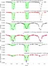 |
Fig. A.17. Same as Fig. A.3, but for three candidates in Sample 2GE-A of light curves modelled with two Gaussians and an ellipsoidal component. The top set shows a case with weak ellipsoidal variability (Gaia DR3 1920242361505734784), the middle set with a mild ellipsoidal component (Gaia DR3 509661748731132800), and the bottom set with very different eclipse depths (Gaia DR3 520547841550454784). |
Sample 2GE-B.
In this sample, the large amplitudes of the ellipsoidal component in the two-Gaussian models dictate the overall morphology of the light curves. The peak-to-peak amplitudes range from 0.11 mag (by definition) to above 0.35 mag (see Fig. A.16, top panel). The Gaussian components, on the other hand, determine the sharpness of the eclipses in the light curve.
The depth of the Gaussian component is typically between half and twice the peak-to-peak amplitude of the ellipsoidal amplitude. Three example light curves are shown in Fig. A.18. In the top example, the Gaussian (depth of 0.15 mag) is less prominent than the ellipsoidal component (peak-to-peak amplitude of 0.25 mag). The middle example shows a case with a stronger Gaussian component (depth of 0.51 mag) than the ellipsoidal amplitude (peak-to-peak amplitude of 0.25 mag). The impact of the Gaussian component on the otherwise sine-like shape of the light curve is clearly visible. The bottom example illustrates a case with a secondary Gaussian that is much shallower than the primary Gaussian. This last case characterises a small fraction of the candidates in Sample 2GE-B, which have Gaussian depth ratios lower than about 0.3. In Fig. A.16 (bottom panel), these are seen to be an extension of the distribution of Sample 2GE-A towards larger ellipsoidal amplitudes.
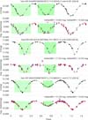 |
Fig. A.18. Same as Fig. A.3, but for three candidates in Sample 2GE-B of light curves modelled with two Gaussians and an ellipsoidal component. The top case shows an example of light curve where the ellipsoidal component is the major contributor to the light-curve shape (Gaia DR3 3444083186030598272), while the second case shows an example with a larger Gaussian depth than the ellipsoidal variability amplitude (Gaia DR3 249126318130979840). The bottom case exemplifies a Sample 2GE-B source with a small depth ratio (of 0.14) between the secondary and primary Gaussian depths. |
Sample 2GE-Z
Only 10% of the models with two Gaussians and a cosine fall in Sample 2GE-Z, which is characterised by eclipse separations deviating from 0.5 by Δ0.5(φecl) > 0.07. The majority of these sources have small ellipsoidal variability amplitudes (Fig. A.15, lower right sample). An analysis based on their Gaussian widths, similarly to what is done in Sect. A.1 for models containing only two Gaussians, suggests that the model components in Sample 2GE-Z may not reflect physical features of binary systems and that further investigation is required before drawing conclusions. The Gaussian widths are indeed widely distributed in the σ1 – σ2 plane, contrary to the distributions of the 2GE-A and 2GE-B samples. Sample 2GE-Z is reminiscent of Samples 2G-X and 2G-Y in Sect. A.1.
Another indication that the Gaussian models of Sample 2GE-Z should be taken with caution comes from their global rankings. The distribution of the rankings of all sources with two Gaussians and a cosine is shown in Fig. A.19 against Δ0.5(φecl). Sample 2GE-Z, defined by Δ0.5(φecl) > 0.07, has a distribution peaked towards low global rankings, while samples 2GE-A and 2GE-B, located at Δ0.5(φecl) < 0.07, are predominantly found at larger rankings. Moreover, the candidates in Sample 2GE-Z that do have large global rankings, have, on average, very shallow secondary Gaussians, as shown in the bottom panel of Fig. A.19. The second eclipse of these models, despite their good global rankings, may therefore be spurious. We note that samples 2GE-A and 2GE-B have, on average, good global rankings. Sample 2GE-Z therefore harbours a variety of cases that require additional investigation before using their two-Gaussian model parameters. Sample 2GE-Z represents only 2% of the full catalogue.
 |
Fig. A.19. Same as Fig. A.15, but for the global ranking versus eclipse phase separation relative to 0.5. Top panel: Density map. Bottom panel: Primary-to-secondary Gaussian depth ratio colour-coded according to the colour scale shown to the right of the panel. |
A.3. Models with only one Gaussian
Sample 1G.
The number of sources whose light-curve model contains only one Gaussian, defining Sample 1G, amounts to 1.7% of the full catalogue. Eccentric systems can result in the occurrence of only one eclipse. The detection of only one eclipse can also happen if the light emitted by the companion in the considered photometric band is below the instrument detection limit. But such a situation can also come about if the period is wrong (typically by a factor of two), or if there are insufficient observations in the eclipse(s). Three example light curves are shown in Fig. A.20. In the top example, the period may be too small by a factor of two. In the second example, the secondary eclipse may lack sufficient observations. In the third example, the lack of sufficient eclipse coverage leads to an unconstrained eclipse depth, resulting in an excessively large depth. This last case is similar to what was noticed in Sect. A.1 for some sources in samples 2G-A and 2G-D. The distribution of the primary eclipse depth versus eclipse duration is shown in the bottom panel of Fig. A.6 for Sample 1G. In summary, the eclipsing-binary candidates in Sample 1G require additional investigation in order to confirm their properties.
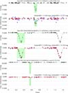 |
Fig. A.20. Same as Fig. A.3, but for three candidates in Sample 1G of light curves modelled with only one Gaussian. The top set (Gaia DR3 5524068296237910272) shows a case where the period is probably a factor of two too small, the second set (Gaia DR3 3033226683222463872) shows a case where observation may be missing at the phase window of the second eclipse, and the third case (Gaia DR3 5541461814286341632) illustrates a case where the lack of sufficient phase coverage within an eclipse leads to an overestimation of the eclipse depth. |
A.4. Models with one Gaussian and an ellipsoidal component
Sample 1GE.
For 2.2% of the sources in the catalogue, the G light curve is modelled with one Gaussian and an ellipsoidal component. These sources define Sample 1GE, and are comparable to sources modelled with two Gaussians and an ellipsoidal component, but with a secondary eclipse (on top of the ellipsoidal variability) that is too faint to be detected, leading to the absence of a second Gaussian in the model. The Gaussian depth is shown in Fig. A.21 versus the peak-to-peak amplitude of the ellipsoidal variability. A comparison of this figure with the similar figure for models containing two Gaussians (Fig. A.16, top panel) confirms that Sample 1GE can be considered to be an extension at small primary Gaussian depths of samples 2GE-A and 2GE-B. The peak-to-peak amplitude distribution of the ellipsoidal component in Sample 1GE is shown by the red histogram in Fig. A.14. Example light curves of sources in this sample are displayed in Fig. A.22.
 |
Fig. A.21. Same as the top panel of Fig. A.16, but for the sample 1GE with one Gaussian component and an ellipsoidal component. The axis scales are kept identical to those in Fig. A.16 for ease of comparison. |
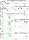 |
Fig. A.22. Same as Fig. A.3, but for three candidates in Sample 1GE of light curves modelled with one Gaussian and an ellipsoidal component. The top, middle, and bottom sets show cases with large (Gaia DR3 5310453356151345408), mild (Gaia DR3 4513043989925301760), and small (Gaia DR3 4052342222634008320) ellipsoidal component relative to the Gaussian depth. The secondary eclipse of the middle case may have gone undetected because of a lack of Gaia measurements at a phase of 0.5 apart from the primary eclipse. |
A.5. Models with only an ellipsoidal component
Sample 0GE.
The remaining candidates in the catalogue are modelled with only a cosine and no Gaussian function, and make up only 2% of the full catalogue. We label them Sample 0GE. In most cases, a purely cosine model is favoured by the automated procedure over a solution involving Gaussians when photometric uncertainties are large. This is shown in Fig. A.23, where the signal-to-noise ratio is plotted versus G magnitude. For comparison, the distribution of the 2GE-B sample is also shown in the figure by six contour lines equally distant on a linear scale. As a result, since photometric uncertainty increases with increasing magnitude, the magnitudes of the 0GE sample are, on average, fainter than any of the other samples containing an ellipsoidal component (see Fig. A.24). The presence of intrinsic scatter in the light curve may also cause the automated procedure to favour a purely cosine model over models containing Gaussian functions.
 |
Fig. A.23. Density map of the S/N (computed as the ratio of the standard deviation over the root-mean-square of the G magnitude uncertainties) versus G magnitude for the sample of candidates modelled with only a cosine function (Sample 0GE). The contours delineate the density of sources in the sample 2GE-B (modelled with two Gaussians and an ellipsoidal component with large amplitude (see text). Six contours are shown on a linear scale of the density of sources on the map. |
 |
Fig. A.24. G magnitude distribution of the various samples containing an ellipsoidal component in their light-curve models, as labeled in the figure The abscissa has been truncated at the bright side for greater visibility. |
An example light curve of a faint (∼18.25 mag in G) 0GE source is shown in Fig. A.25 (top case). The GBP and GRP light curves confirm the ellipsoidal-like variability, though with much larger uncertainties on the measurements. The second example displays another 0GE faint source (∼19.05 mag in G) with a clear sinusoidal-like variability in G, but with no such clear variability in GBP and GRP. Sources like this one require further confirmation of their variability. The last example in Fig. A.25 shows a (rarer) bright case, with G around 13.3 mag.
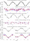 |
Fig. A.25. Same as Fig. A.3, but for three candidates in Sample 0GE (light curves modelled with only a cosine). The first two examples show the most common cases of faint candidates, with (top case, Gaia DR3 5923298253884922624)and without (middle case, Gaia DR3 4037337565429141376) clear confirmation of the variability in the GBP and GRP light curves. The bottom example shows a relatively rare case (in this sample) of a bright candidate (Gaia DR3 5236421790821776256). |
A.6. Summary
Table 3 in the main body of the text summarises the various samples, which are categorised according to the type of binary system expected for the majority of candidates in each one of them. The light curve alone does not always allow us to uniquely identify the type of binary system that it originates from. The light curve of an Algol-type eclipsing binary, for example, in which a star that fills its Roche lobe is much fainter than its companion, can resemble that of a fully detached system. We therefore consider wide versus tight systems without further subclassification. Wide detached systems lead to light curves that are either devoid of ellipsoidal variability (samples 2G-A, 2G-D, 1G) or have a mild ellipsoidal component (2GE-A). Algol-type systems where the secondary is much fainter than the primary would preferentially be classified in this category as well. This first category gathers about one-fourth of the catalogue. The second category contains tighter systems, displaying light curves that have either a predominant ellipsoidal component (samples 2GE-B, 1GE, 0GE), or are described by two wide overlapping Gaussians (2G-B, 2G-C). These represent more than half of the catalogue. We note that the two famous tight systems β Lyr and W UMa belong to Sample 2GE-B (see Fig. 8 in the main body of the article). The third category, containing less than one-fifth of the catalogue, gathers samples 2G-X, 2G-Y, and 2GE-Z. Identifying the nature of the majority of the candidates therein will require further investigation. The grouping of the samples in these three categories is supported by their period distributions shown in Fig. 16. The samples in the first category (2G-A, 2GE-A, 2G-D, 1G) all display wide period distributions reaching values above 10 days (top panel in the figure), as expected for wide systems, while the samples in the second category have period distributions peaking below 0.5 days (second and third panels in the figure), as expected for tight systems. The distributions of the period versus magnitude for all samples are shown in Fig. A.26. Likewise, the distributions of their global ranking versus magnitude are shown in Fig. A.27. The abscissa and ordinate scales are kept identical in all panels of each figure to enable straightforward comparison.
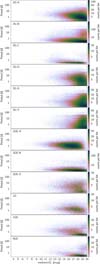 |
Fig. A.26. Density maps of period versus G magnitude for the various samples defined in Table A.1. |
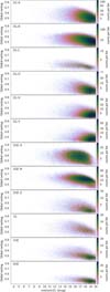 |
Fig. A.27. Same as Fig. A.26, but for global ranking versus G magnitude. |
Several additional figures per sample are shown in Figs. A.28 to A.30. Figure A.28 shows the distribution of the number of cleaned measurements in the G light curves versus orbital period for each sample. Figure A.29 complements Fig. A.28 by showing the distribution of the global ranking in this plane. These two figures are discussed in Sect. 3.4 of the main text. Figure A.30, on the other hand, shows the Spearman correlation ripd, G between source image goodness of fit and the G time series, versus period for each sample, and is discussed in Sect. 3.5 of the main text.
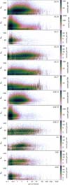 |
Fig. A.28. Density maps of the number of good measurements in the G light curve versus period for the various samples defined in Table A.1. |
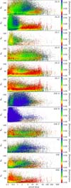 |
Fig. A.29. Same as Fig. A.28, but colour-coded with the median of the global ranking in each cell. The colour scale shown to the right of each figure is truncated at both ends for improved visibility. |
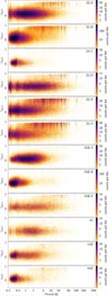 |
Fig. A.30. Density map of the ripd, G correlation versus orbital period for each sample. |
The categorisation presented in Table 3 is not intended to provide a thorough classification of the two million eclipsing-binary candidates, a task that would require additional analysis. Rather, it offers a convenient, quick analysis and overview of the catalogue content. It must also be stressed that the definition of the samples as given in Table A.1 is based on well-defined cuts on σp, σs, Aell and Δ0.5(φecl), which introduces an additional source of uncertainty in the classification.
Appendix B: Eccentricity proxy
A proxy for the eccentricity can be derived using the two-Gaussian model results based on the derived relative locations and durations of the eclipses. At small eccentricities, the projected eccentricity eproxycos ω can be approximated from the phase separation of the eclipses with
where eproxy is the eccentricity proxy and ω is the periastron argument. Equation B.1 is readily computable from the derived model parameters. In addition to eclipse locations, the models also provide the durations wecl, 1 and wecl, 2 of the primary and secondary eclipses, respectively. From these parameters, eproxysin ω can be computed using
The eccentricity is then easily derived from Eqs. B.1 and B.2, and writes
The uncertainty ε(eproxy) on the eccentricity proxy can be computed from Eq. B.3 by propagation of the uncertainties ε(φecl, 1), ε(φecl, 2), ε(wecl, 1) and ε(wecl, 2) of φecl, 1, φecl, 2, wecl, 1 and wecl, 2, respectively. Assuming these uncertainties are uncorrelated, we obtain
The eccentricities are shown versus period in Fig. B.1 for the various samples defined in Sect. 3.1 that contain two Gaussians in their light-curve models. The samples displayed in the figure are limited to the candidates analysed in Sect. 5 that have good parallaxes (uncertainties better than 15%), corrected BP+RP flux excess factor C* smaller than 0.5, and either have global rankings larger than 0.6 or belong to group 2G-C. Figure B.1 shows that most candidates in groups with potential tidal interactions (groups 2G-B, 2G-C, 2GE-A and 2GE-B) have eccentricity proxies smaller than 0.1. The uncertainties on these values, shown versus eccentricity in Fig. B.2, can be as large as 0.15 even at these small eccentricity proxies. These small eccentricities are therefore compatible with circularised systems.
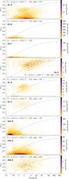 |
Fig. B.1. Density maps of the eccentricity proxy versus orbital period for samples with good parallaxes and global rankings as defined in the text. The dashed lines are Eq. (4.4) from Mazeh (2008) with E = 0.98, A = 3.25, B = 6.3, and C = 0.23. The axis ranges are truncated for improved visibility. |
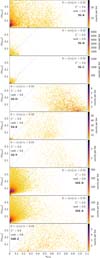 |
Fig. B.2. Same as Fig. B.1, but for the uncertainty on the eccentricity proxy versus the eccentricity proxy. The dashed lines are one-to-one lines. |
 |
Fig. B.3. Histograms of the relative uncertainty on the eccentricity proxy for various samples with conditions on the parallax, corrected BP+RP flux excess factor and global ranking as written in the figure. |
In contrast, large eccentricity proxies (eproxy ≳ 0.3) are found in group 2G-A (top panel in Fig. B.1), which contains well-detached systems with no tidal effect. In particular, many short-period systems are seen to have large eccentricity proxies, contrary to the expectation of them being circularised. This can be seen in the figure, where the eccentricity limit at any given orbital period —above which systems are expected to be circularised— is shown by the dashed blue line based on Eq. (4.4) of Mazeh (2008; with E = 0.98, A = 3.25, B = 6.3 and C = 0.23). However, a careful analysis of the systems with eccentricities larger than this limit, performed in Sect. 5 of the main body of this article, concludes that the eccentricity and/or orbital period of these systems are incorrect. Caution must therefore be taken in the interpretation of the two-Gaussian model results when analysing specific cases.
Large eccentricity proxies are also derived for candidates in groups 2G-D, 2G-X, 2G-Y, and 2GE-Z (Fig. B.1). These groups are shown in Sect. 3.1 to have unreliable light-curve models. Their large eccentricities are therefore mostly spurious, and require confirmation on a case-by-case basis.
Appendix C: Additional figures
Figures C.1 to C.5 show the GBP and GRP folded light curves of the eclipsing binaries displayed in Sect. 3.1, except for V614 Ven, for which the GBP and GRP light curves are shown in Fig. 4.
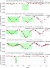 |
Fig. C.1. GBP and GRP folded light curves of the eclipsing binaries whose G are shown Fig. 5 in the main body of the article. The GBP and GRP magnitudes are shifted by a value equal to the median magnitudes of their respective light curves, given in the top of each panel. The dotted line represents the two-Gaussian models determined from the G light curves, with the green areas indicating the derived eclipse durations. |
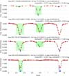 |
Fig. C.2. Same as Fig. C.1, but for the eclipsing binaries whose G light curves are shown in Fig. 7 in the main body of the article. |
 |
Fig. C.3. Same as Fig. C.1, but for the eclipsing binaries whose G light curves are shown in Fig. 8 in the main body of the article. |
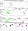 |
Fig. C.4. Same as Fig. C.1, but for the eclipsing binaries whose G light curves are shown in Fig. 9 in the main body of the article. |
 |
Fig. C.5. Same as Fig. C.1, but for the eclipsing binaries whose G light curves are shown in Fig. 10 in the main body of the article. |
Figure C.6 shows the sky distribution of the number of good G-band measurements of all sources in the Gaia DR3 catalogue of eclipsing-binary candidates. This figure is to be compared to the sky distribution of these candidates shown in Fig. 1 in the main body of this article.
 |
Fig. C.6. Sky distribution (Galactic coordinates) of the number NG of FOV observations selected for variability analysis in the G light curves of the Gaia eclipsing binaries, colour-coded according to the colour scale shown to the right of the figure. |
Figure C.7 shows the magnitude distributions of the OGLE4 samples of eclipsing binaries used in Sect. 4.2 to estimate the completeness of the Gaia catalogue. The figure plots the distributions of the OGLE4 sources in the I, V and G bands separately for the OGLE4 samples towards the LMC (top panel), SMC (middle panel), and Galactic Bulge (bottom panel). The G distribution of the Gaia – OGLE4 cross-matches is also shown in each panel by the filled blue histograms.
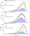 |
Fig. C.7. Magnitude distributions of OGLE4 eclipsing binaries that have a GaiaG magnitude. The distributions are given for the LMC (top panel), the SMC (middle panel), and the Galactic bulge (bottom panel). The OGLE4 I and V magnitudes are shown with a thin green and a dashed grey line, respectively, and their GaiaG magnitude is shown with a thick red line. The G distribution of the subset present in the Gaia catalogue of eclipsing binaries is shown by the filled blue histogram. |
Figure C.8 shows the observational diagram of the sample of eclipsing-binary candidates with parallax uncertainties better than 15%, with the absolute magnitudes MG shifted by 0.75 mag to compare with the distribution of a random sample of Gaia DR3 sources. For this purpose, the contour lines of the random ten million sources shown in the top panel of Fig. 36 (see Sect. 5 in the main text of the article) have not been shifted by 0.75 mag. Figure C.9 shows the light curves of two Gaia candidates discussed in Sect. 5, folded with the ASAS-SN periods of the respective cross-matched ASAS-SN sources.
 |
Fig. C.8. Same as second panel of Fig. 36 in the main body of the text, but with the absolute magnitude MG shifted by 0.75 mag. The contour lines representing the ten million random sample shown in the top panel of Fig. 36 have not been shifted by 0.75 mag. |
 |
Fig. C.9. Light curves of Gaia DR3 4524651705941314432 and Gaia DR3 5712304991851559040 shown in Fig. 41 in the main body of the text, folded with the periods published by the ASAS-SN survey for the respective cross-matches (ASASSN-V J075432.26-211826.4 with P = 3.3972697 d, and ASASSN-V J184156.16+192755.8 with 5.9965616 d, respectively). |
Appendix D: Full acknowledgements
This work presents results from the European Space Agency (ESA) space mission Gaia. Gaia data are being processed by the Gaia Data Processing and Analysis Consortium (DPAC). Funding for the DPAC is provided by national institutions, in particular the institutions participating in the Gaia MultiLateral Agreement (MLA). The Gaia mission website is https://www.cosmos.esa.int/gaia. The Gaia archive website is https://archives.esac.esa.int/gaia.
The Gaia mission and data processing have financially been supported by, in alphabetical order by country:
-
the Algerian Centre de Recherche en Astronomie, Astrophysique et Géophysique of Bouzareah Observatory;
-
the Austrian Fonds zur Förderung der wissenschaftlichen Forschung (FWF) Hertha Firnberg Programme through grants T359, P20046, and P23737;
-
the BELgian federal Science Policy Office (BELSPO) through various PROgramme de Développement d’Expériences scientifiques (PRODEX) grants and the Polish Academy of Sciences - Fonds Wetenschappelijk Onderzoek through grant VS.091.16N, and the Fonds de la Recherche Scientifique (FNRS), and the Research Council of Katholieke Universiteit (KU) Leuven through grant C16/18/005 (Pushing AsteRoseismology to the next level with TESS, GaiA, and the Sloan DIgital Sky SurvEy – PARADISE);
-
the Brazil-France exchange programmes Fundação de Amparo à Pesquisa do Estado de São Paulo (FAPESP) and Coordenação de Aperfeicoamento de Pessoal de Nível Superior (CAPES) - Comité Français d’Evaluation de la Coopération Universitaire et Scientifique avec le Brésil (COFECUB);
-
the Chilean Agencia Nacional de Investigación y Desarrollo (ANID) through Fondo Nacional de Desarrollo Científico y Tecnológico (FONDECYT) Regular Project 1210992 (L. Chemin);
-
the National Natural Science Foundation of China (NSFC) through grants 11573054, 11703065, and 12173069, the China Scholarship Council through grant 201806040200, and the Natural Science Foundation of Shanghai through grant 21ZR1474100;
-
the Tenure Track Pilot Programme of the Croatian Science Foundation and the École Polytechnique Fédérale de Lausanne and the project TTP-2018-07-1171 ‘Mining the Variable Sky’, with the funds of the Croatian-Swiss Research Programme;
-
the Czech-Republic Ministry of Education, Youth, and Sports through grant LG 15010 and INTER-EXCELLENCE grant LTAUSA18093, and the Czech Space Office through ESA PECS contract 98058;
-
the Danish Ministry of Science;
-
the Estonian Ministry of Education and Research through grant IUT40-1;
-
the European Commission’s Sixth Framework Programme through the European Leadership in Space Astrometry (https://www.cosmos.esa.int/web/gaia/elsa-rtn-programme) Marie Curie Research Training Network (MRTN-CT-2006-033481), through Marie Curie project PIOF-GA-2009-255267 (Space AsteroSeismology & RR Lyrae stars, SAS-RRL), and through a Marie Curie Transfer-of-Knowledge (ToK) fellowship (MTKD-CT-2004-014188); the European Commission’s Seventh Framework Programme through grant FP7-606740 (FP7-SPACE-2013-1) for the Gaia European Network for Improved data User Services (https://gaia.ub.edu/twiki/do/view/GENIUS/) and through grant 264895 for the Gaia Research for European Astronomy Training (https://www.cosmos.esa.int/web/gaia/great-programme) network;
-
the European Cooperation in Science and Technology (COST) through COST Action CA18104 ‘Revealing the Milky Way with Gaia (MW-Gaia)’;
-
the European Research Council (ERC) through grants 320360, 647208, and 834148 and through the European Union’s Horizon 2020 research and innovation and excellent science programmes through Marie Skłodowska-Curie grant 745617 (Our Galaxy at full HD – Gal-HD) and 895174 (The build-up and fate of self-gravitating systems in the Universe) as well as grants 687378 (Small Bodies: Near and Far), 682115 (Using the Magellanic Clouds to Understand the Interaction of Galaxies), 695099 (A sub-percent distance scale from binaries and Cepheids – CepBin), 716155 (Structured ACCREtion Disks – SACCRED), 951549 (Sub-percent calibration of the extragalactic distance scale in the era of big surveys – UniverScale), and 101004214 (Innovative Scientific Data Exploration and Exploitation Applications for Space Sciences – EXPLORE);
-
the European Science Foundation (ESF), in the framework of the Gaia Research for European Astronomy Training Research Network Programme (https://www.cosmos.esa.int/web/gaia/great-programme);
-
the European Space Agency (ESA) in the framework of the Gaia project, through the Plan for European Cooperating States (PECS) programme through contracts C98090 and 4000106398/12/NL/KML for Hungary, through contract 4000115263/15/NL/IB for Germany, and through PROgramme de Développement d’Expériences scientifiques (PRODEX) grant 4000127986 for Slovenia;
-
the Academy of Finland through grants 299543, 307157, 325805, 328654, 336546, and 345115 and the Magnus Ehrnrooth Foundation;
-
the French Centre National d’Études Spatiales (CNES), the Agence Nationale de la Recherche (ANR) through grant ANR-10-IDEX-0001-02 for the ‘Investissements d’avenir’ programme, through grant ANR-15-CE31-0007 for project ‘Modelling the Milky Way in the Gaia era’ (MOD4Gaia), through grant ANR-14-CE33-0014-01 for project ‘The Milky Way disc formation in the Gaia era’ (ARCHEOGAL), through grant ANR-15-CE31-0012-01 for project ‘Unlocking the potential of Cepheids as primary distance calibrators’ (UnlockCepheids), through grant ANR-19-CE31-0017 for project ‘Secular evolution of galxies’ (SEGAL), and through grant ANR-18-CE31-0006 for project ‘Galactic Dark Matter’ (GaDaMa), the Centre National de la Recherche Scientifique (CNRS) and its SNO Gaia of the Institut des Sciences de l’Univers (INSU), its Programmes Nationaux: Cosmologie et Galaxies (PNCG), Gravitation Références Astronomie Métrologie (PNGRAM), Planétologie (PNP), Physique et Chimie du Milieu Interstellaire (PCMI), and Physique Stellaire (PNPS), the ‘Action Fédératrice Gaia’ of the Observatoire de Paris, the Région de Franche-Comté, the Institut National Polytechnique (INP) and the Institut National de Physique nucléaire et de Physique des Particules (IN2P3) co-funded by CNES;
-
the German Aerospace Agency (Deutsches Zentrum für Luft- und Raumfahrt e.V., DLR) through grants 50QG0501, 50QG0601, 50QG0602, 50QG0701, 50QG0901, 50QG1001, 50QG1101, 50QG1401, 50QG1402, 50QG1403, 50QG1404, 50QG1904, 50QG2101, 50QG2102, and 50QG2202, and the Centre for Information Services and High Performance Computing (ZIH) at the Technische Universität Dresden for generous allocations of computer time;
-
the Hungarian Academy of Sciences through the Lendület Programme grants LP2014-17 and LP2018-7 and the Hungarian National Research, Development, and Innovation Office (NKFIH) through grant KKP-137523 (‘SeismoLab’);
-
the Science Foundation Ireland (SFI) through a Royal Society - SFI University Research Fellowship (M. Fraser);
-
the Israel Ministry of Science and Technology through grant 3-18143 and the Tel Aviv University Center for Artificial Intelligence and Data Science (TAD) through a grant;
-
the Agenzia Spaziale Italiana (ASI) through contracts I/037/08/0, I/058/10/0, 2014-025-R.0, 2014-025-R.1.2015, and 2018-24-HH.0 to the Italian Istituto Nazionale di Astrofisica (INAF), contract 2014-049-R.0/1/2 to INAF for the Space Science Data Centre (SSDC, formerly known as the ASI Science Data Center, ASDC), contracts I/008/10/0, 2013/030/I.0, 2013-030-I.0.1-2015, and 2016-17-I.0 to the Aerospace Logistics Technology Engineering Company (ALTEC S.p.A.), INAF, and the Italian Ministry of Education, University, and Research (Ministero dell’Istruzione, dell’Università e della Ricerca) through the Premiale project ‘MIning The Cosmos Big Data and Innovative Italian Technology for Frontier Astrophysics and Cosmology’ (MITiC);
-
the Netherlands Organisation for Scientific Research (NWO) through grant NWO-M-614.061.414, through a VICI grant (A. Helmi), and through a Spinoza prize (A. Helmi), and the Netherlands Research School for Astronomy (NOVA);
-
the Polish National Science Centre through HARMONIA grant 2018/30/M/ST9/00311 and DAINA grant 2017/27/L/ST9/03221 and the Ministry of Science and Higher Education (MNiSW) through grant DIR/WK/2018/12;
-
the Portuguese Fundação para a Ciência e a Tecnologia (FCT) through national funds, grants SFRH/BD/128840/2017 and PTDC/FIS-AST/30389/2017, and work contract DL 57/2016/CP1364/CT0006, the Fundo Europeu de Desenvolvimento Regional (FEDER) through grant POCI-01-0145-FEDER-030389 and its Programa Operacional Competitividade e Internacionalização (COMPETE2020) through grants UIDB/04434/2020 and UIDP/04434/2020, and the Strategic Programme UIDB/00099/2020 for the Centro de Astrofísica e Gravitação (CENTRA);
-
the Slovenian Research Agency through grant P1-0188;
-
the Spanish Ministry of Economy (MINECO/FEDER, UE), the Spanish Ministry of Science and Innovation (MICIN), the Spanish Ministry of Education, Culture, and Sports, and the Spanish Government through grants BES-2016-078499, BES-2017-083126, BES-C-2017-0085, ESP2016-80079-C2-1-R, ESP2016-80079-C2-2-R, FPU16/03827, PDC2021-121059-C22, RTI2018-095076-B-C22, and TIN2015-65316-P (‘Computación de Altas Prestaciones VII’), the Juan de la Cierva Incorporación Programme (FJCI-2015-2671 and IJC2019-04862-I for F. Anders), the Severo Ochoa Centre of Excellence Programme (SEV2015-0493), and MICIN/AEI/10.13039/501100011033 (and the European Union through European Regional Development Fund ‘A way of making Europe’) through grant RTI2018-095076-B-C21, the Institute of Cosmos Sciences University of Barcelona (ICCUB, Unidad de Excelencia ‘María de Maeztu’) through grant CEX2019-000918-M, the University of Barcelona’s official doctoral programme for the development of an R+D+i project through an Ajuts de Personal Investigador en Formació (APIF) grant, the Spanish Virtual Observatory through project AyA2017-84089, the Galician Regional Government, Xunta de Galicia, through grants ED431B-2021/36, ED481A-2019/155, and ED481A-2021/296, the Centro de Investigación en Tecnologías de la Información y las Comunicaciones (CITIC), funded by the Xunta de Galicia and the European Union (European Regional Development Fund – Galicia 2014-2020 Programme), through grant ED431G-2019/01, the Red Española de Supercomputación (RES) computer resources at MareNostrum, the Barcelona Supercomputing Centre - Centro Nacional de Supercomputación (BSC-CNS) through activities AECT-2017-2-0002, AECT-2017-3-0006, AECT-2018-1-0017, AECT-2018-2-0013, AECT-2018-3-0011, AECT-2019-1-0010, AECT-2019-2-0014, AECT-2019-3-0003, AECT-2020-1-0004, and DATA-2020-1-0010, the Departament d’Innovació, Universitats i Empresa de la Generalitat de Catalunya through grant 2014-SGR-1051 for project ‘Models de Programació i Entorns d’Execució Parallels’ (MPEXPAR), and Ramon y Cajal Fellowship RYC2018-025968-I funded by MICIN/AEI/10.13039/501100011033 and the European Science Foundation (‘Investing in your future’);
-
the Swedish National Space Agency (SNSA/Rymdstyrelsen);
-
the Swiss State Secretariat for Education, Research, and Innovation through the Swiss Activités Nationales Complémentaires and the Swiss National Science Foundation through an Eccellenza Professorial Fellowship (award PCEFP2_194638 for R. Anderson);
-
the United Kingdom Particle Physics and Astronomy Research Council (PPARC), the United Kingdom Science and Technology Facilities Council (STFC), and the United Kingdom Space Agency (UKSA) through the following grants to the University of Bristol, the University of Cambridge, the University of Edinburgh, the University of Leicester, the Mullard Space Sciences Laboratory of University College London, and the United Kingdom Rutherford Appleton Laboratory (RAL): PP/D006511/1, PP/D006546/1, PP/D006570/1, ST/I000852/1, ST/J005045/1, ST/K00056X/1, ST/K000209/1, ST/K000756/1, ST/L006561/1, ST/N000595/1, ST/N000641/1, ST/N000978/1, ST/N001117/1, ST/S000089/1, ST/S000976/1, ST/S000984/1, ST/S001123/1, ST/S001948/1, ST/S001980/1, ST/S002103/1, ST/V000969/1, ST/W002469/1, ST/W002493/1, ST/W002671/1, ST/W002809/1, and EP/V520342/1.
The Ground Based Optical Tracking (GBOT) programme uses observations collected at (i) the European Organisation for Astronomical Research in the Southern Hemisphere (ESO) with the VLT Survey Telescope (VST), under ESO programmes 092.B-0165, 093.B-0236, 094.B-0181, 095.B-0046, 096.B-0162, 097.B-0304, 098.B-0030, 099.B-0034, 0100.B-0131, 0101.B-0156, 0102.B-0174, and 0103.B-0165; and (ii) the Liverpool Telescope, which is operated on the island of La Palma by Liverpool John Moores University in the Spanish Observatorio del Roque de los Muchachos of the Instituto de Astrofísica de Canarias with financial support from the United Kingdom Science and Technology Facilities Council, and (iii) telescopes of the Las Cumbres Observatory Global Telescope Network.
All Tables
Data fields in the Gaia DR3 table of eclipsing binaries (Gaia DR3 table vari_eclipsing_binary), with their units (Col. 2), the mathematical symbol used in this paper (if used, Col. 3), and a short description (Col. 4).
Some statistics on the period comparison between the Gaia DR3 catalogue of eclipsing binaries and literature data.
Number of Gaia DR3 eclipsing-binary candidates in selected sky areas of the LMC and Galactic Bulge.
All Figures
 |
Fig. 1. Sky-density map of the Gaia catalogue of eclipsing binaries in Galactic coordinates. The map is colour-coded according to the colour scale shown to the right of the figure. |
| In the text | |
 |
Fig. 2. Distribution of G magnitude of the full sample (black histogram) and of the samples with global ranking larger than 0.6 (filled green histogram) and smaller than 0.5 (red spiked histogram). The abscissa scale is truncated at the lower side for improved visibility. |
| In the text | |
 |
Fig. 3. Schematic representation of the two-Gaussian model parameters used in Eq. (3) to fit folded light curves of eclipsing binaries. The ordinate represents magnitude in reverse order. Three cases are shown with their primary eclipses (arbitrarily) located at phase 0.2. Case (a) illustrates the modelling of a well-detached eccentric system using two non-overlapping Gaussians. Case (b) shows a very tight circular system modelled with two overlapping Gaussians. Case (c) represents a tight circular system with an out-of-eclipse ellipsoidal variation modelled with a cosine component. The red dashed horizontal line in each panel indicates the value of the constant C in Eq. (3). The green areas delimit the eclipse durations. The thin black dotted lines in the middle and bottom panels show the individual Gaussian and/or cosine components of the two-Gaussian models. The thick black solid lines show the resulting two-Gaussian models. |
| In the text | |
 |
Fig. 4. Folded light curves of V614 Ven. Top panel: G light curve. The two-Gaussian model is superposed as a dotted line. The green areas indicate the derived eclipse durations. Bottom panel: GBP and GRP light curves (blue and red dots, respectively), shifted by a value equal to their respective median magnitudes as written in the top of the panel. The GRP light curve is plotted on top of the GBP one, the former therefore hiding the latter when the measurements are at the same ordinate. The dotted model and green areas shown in the bottom panel are the ones from the G light curve shifted to match zero median magnitude. The Gaia period, global ranking, and the light-curve classification (in brackets; see text) are given in the title of the figure after the Gaia DR3 ID and GCVS name. |
| In the text | |
 |
Fig. 5. Same as the top panel of Fig. 4, but for additional eclipsing binaries for which the G light curves are modelled with only two Gaussians. From top to bottom: SW Cyg, V745 Cep, 1687 Aql, NS Cam, and KS Eri. |
| In the text | |
 |
Fig. 6. Distribution of the derived eclipse-depth ratio (secondary over primary) for the various samples with two Gaussians in their light-curve models without (top and middle panels) or with (bottom panel) an ellipsoidal component, as labelled in the panels (see text). The histograms are area-normalised. |
| In the text | |
 |
Fig. 7. Same as top panel of Fig. 4, but for sources with light curves modelled with two Gaussians and a cosine of small to medium amplitude. From top to bottom: AO Ser, DN Cas, MU Cyg, and HN Cas. |
| In the text | |
 |
Fig. 8. Same as top panel of Fig. 4, but for sources with light curves modelled with two Gaussians and a cosine of large amplitude. From top to bottom: β Lyr and W UMa. |
| In the text | |
 |
Fig. 9. Same as top panel of Fig. 4, but for sources with light curves modelled with only one Gaussian (KN And, top panel), one Gaussian and a cosine (V379 Per in second panel and RZ Col in third panel), or only a cosine (DU Car, bottom panel). No green area is displayed for eclipses that are not modelled with a Gaussian component in the light-curve model. |
| In the text | |
 |
Fig. 10. Same as top panel of Fig. 4, but for additional sources with light curves modelled with at least two Gaussians. From top to bottom: AE Mon, V444 Cyg and RU Gem. |
| In the text | |
 |
Fig. 11. Distribution of the global ranking of DR3 EB candidates. The full sample is displayed in thick grey, with the candidates therein that have a cross-match with known eclipsing binaries in the literature shown in thin black. The sample with positive parallax uncertainties better than 15% is displayed in thick green, with the candidates therein with a literature cross-match shown in thin cyan. |
| In the text | |
 |
Fig. 12. Density map of the S/N of the G time series (standard deviation of the measurements divided by the root mean square of their uncertainties) of all eclipsing-binary candidates versus their global ranking. The density in the map is colour coded according to the colour scale shown to the right of the figure. |
| In the text | |
 |
Fig. 13. Same as Fig. 6, but for the global ranking. The histograms of the samples are displayed in two panels as labelled in the panels. |
| In the text | |
 |
Fig. 14. Distribution of the orbital periods of the DR3 eclipsing-binary candidates. The full sample is displayed with a black line, and the sample with global ranking higher than 0.6 is shown in green. The top panel shows the number of counts per bin on a linear scale, while the bottom panel shows them on a logarithmic scale. |
| In the text | |
 |
Fig. 15. Density map of the orbital period versus global ranking of the DR3 eclipsing-binary candidates. |
| In the text | |
 |
Fig. 16. Period distributions of various samples according to their two-model parameters as labelled in the panels (see text). The filled grey histograms represent the combined samples in each panel. |
| In the text | |
 |
Fig. 17. Density map of the number of good measurements in the G band versus global ranking. |
| In the text | |
 |
Fig. 18. Number of good measurements in the G band versus period plane. Top panel: density map. Bottom panel: median value of the global ranking in each cell of the figure, colour-coded according to the colour scale shown to the right of the panel. |
| In the text | |
 |
Fig. 19. Same as Fig. 4 for two additional candidates in group 2G-A. Top panel: candidate with a low number of measurements in G and high global ranking. Bottom panel: candidate with a large number of measurements in G and low global ranking. |
| In the text | |
 |
Fig. 20. Density map of the ripd, G correlation (providing an indication of the possible strength of a scan-angle-dependent signal in the photometric time series) versus global ranking of the full catalogue. |
| In the text | |
 |
Fig. 21. Same as Fig. 20, but versus orbital period and with a more restricted ordinate range for better visibility. |
| In the text | |
 |
Fig. 22. Cumulative distribution of the phase deviation rP, lit at the end of the observation obtained when adopting the literature period Plit instead of the Gaia period PGaia (see Eq. (6)). The sample of Gaia eclipsing-binary candidates that are also classified as eclipsing binaries in the literatures is shown by the filled grey histogram, and the sample which has literature cross-matches but with a classification other than eclipsing binary in the literature is shown by the red histogram. |
| In the text | |
 |
Fig. 23. Gaia period versus literature period for all Gaia DR3 eclipsing-binary candidates that have a cross-match in the literature. Top panel: candidates also identified as eclipsing binaries in the literature. Bottom panel: candidates not classified as eclipsing binaries in the literature. The imprints of literature catalogues are visible in the distributions of Plit (see text). |
| In the text | |
 |
Fig. 24. Sky distributions (density maps) in equatorial coordinates of eclipsing-binary candidates around the LMC. The panels show, from top to bottom, Gaia DR3 candidates, OGLE4 candidates, the Gaia-OGLE4 cross-matches (2 arcsecs radius), and the new Gaia candidates with respect to OGLE4. Sources highlighted by filled circles in the bottom panel have their G light curves displayed in Figs. 31 and 32; they are located in the bar of the LMC for the cyan markers and outside the bar for the blue markers. The orange area delineates the subregion of the sky used in the text to compute the fraction of Gaia new candidates towards the LMC. |
| In the text | |
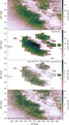 |
Fig. 25. Same as Fig. 24, but towards the Galactic Bulge. |
| In the text | |
 |
Fig. 26. Same as Fig. 24, but for OGLE4 sources in the Galactic Bulge that have no source counterpart in the Gaia DR3 archive. |
| In the text | |
 |
Fig. 27. Median G magnitude distributions of Gaia eclipsing binaries in specific regions of the sky. Top panel: sky region towards the LMC shown in Fig. 24. Bottom panel: sky region towards the Galactic Bulge shown in Fig. 25. The black histograms show all Gaia DR3 eclipsing-binary candidates in the given sky area. The sources among them that have or do not have a cross-match (2 arcsec radius) with the OGLE4 catalogue of eclipsing binaries are shown by the green and red histograms, respectively. The blue histograms are the distributions of sources with no OGLE4 cross-match but a cross match with eclipsing-binary candidates identified in other surveys. The abscissa range is truncated on the bright side for greater visibility. |
| In the text | |
 |
Fig. 28. Same as Fig. 27, but for the global ranking. |
| In the text | |
 |
Fig. 29. Same as Fig. 21, but for sources in the LMC. Top panel: sources detected as eclipsing binaries by OGLE4. Middle panel: new candidates with respect to OGLE4. Bottom panel: new candidates with respect to OGLE4 in the red clump. |
| In the text | |
 |
Fig. 30. Colour–magnitude (top row) and BP+RP flux excess factor versus colour (bottom row) diagrams of the Gaia eclipsing binaries in the sky area towards the LMC shown in Fig. 24. Left panels: new Gaia eclipsing-binary candidates with respect to the OGLE4 catalogue of LMC eclipsing binaries. Middle panels:Gaia sources with a cross-match (2 arcsec radius) with the OGLE4 catalogue. Right panels: Gaia candidates having no cross-match with the OGLE4 candidates but a cross-match with EB candidates in other surveys. The colour of each bin is proportional to the number of counts per bin according to the colour scales shown to the right for each row. Sources highlighted by filled circles have their G light curves displayed in Figs. 31 and 32; they are located in the bar of the LMC for blue circle markers and outside the bar for cyan diamond markers. The axes ranges have been truncated for greater visibility. |
| In the text | |
 |
Fig. 31. Same as top panel of Fig. 4, but for five Gaia candidates outside the LMC bar that are not present in the OGLE4 catalogues of eclipsing binaries, sorted with increasing GBP − GRP colour from top to bottom. The sources are Gaia DR3 4655269942119876864, 4651511051157939968, 4651581458546544000, 4651853274236480256, 4651018852223135104; their sky positions are identified in Fig. 24. |
| In the text | |
 |
Fig. 32. Same as Fig. 31, but for six Gaia candidates in the LMC bar. The sources are Gaia DR3 4657899076482979328, 4658068847785992064, 4657993978084740992, 4657143097661657728, 4657909281189517056, 4657914336358760448. |
| In the text | |
 |
Fig. 33. BP+RP flux excess factor versus colour of the Gaia eclipsing binaries in the sky area towards the Galactic Bulge shown in Fig. 25. Top panel: Gaia candidates with OGLE4 cross-matches. Bottom panel: Gaia candidates with no OGLE4 cross-match. The axes ranges have been truncated for greater visibility. |
| In the text | |
 |
Fig. 34. Corrected BP+RP flux excess factor versus colour of Gaia DR3 eclipsing binaries with positive parallax uncertainties better than 15%. Median values of GBP, GRP, and G are used in all quantities. The axis ranges have been truncated for greater visibility. |
| In the text | |
 |
Fig. 35. Parallax in milliarcseconds versus median(G) of Gaia DR3 eclipsing binaries with positive parallax uncertainties better than 15% and corrected BP+RP flux excess factor smaller than 0.5. |
| In the text | |
 |
Fig. 36. Observational HR diagrams of Gaia DR3 stars with good parallaxes. Top panel: density map of a random sample of ten million stars with parallax uncertainties better than 5% and additional conditions on the number of measurements and source image quality (see text). The yellow lines are evolution tracks of, from bottom to top, 0.8, 1, 1.5, and 2 M⊙ solar-metallicity stellar models from Ekström et al. (2012). Second panel: density map of Gaia eclipsing-binary candidates with parallax uncertainties better than 15% and corrected BP+RP flux excess factors less than 0.5. Contour lines (logarithmic scale) of the sample shown in the top panel are drawn in grey. Third panel: same as second panel, but colour-coded with the median value of the orbital period in each bin. Bottom panel: same as second panel, but colour-coded with the median value of the global ranking in each bin. Median values of the GBP, GRP, and G cleaned time series are used in all panels except in the top one, where mean values are used due to the unavailability of median values for all sources in Gaia DR3. The colours in the figures are coded according to the colour scales to the right of each panel. The ranges of the axes and colour scales are truncated for greater visibility. |
| In the text | |
 |
Fig. 37. Same as third panel of Fig. 36, but for the subset with global rankings higher then 0.6 or belonging to the group 2G-C. |
| In the text | |
 |
Fig. 38. Period distributions of the good parallax sample. The filled grey histogram represents the full distribution, while the orange, blue, magenta, red, and green histograms represent the 2G-A, 2G-B, 2G-C, 2GE-A, and 2GE-B subsamples, respectively. Top panel: all candidates in the good parallax sample with C* < 0.5. Bottom panel: same as top panel, but restricted to candidates with global rankings larger than 0.6 except for group 2G-C. |
| In the text | |
 |
Fig. 39. Eccentricity proxy versus orbital period of Sample 2G-A eclipsing binaries (well-detached and without ellipsoidal component) that are brighter than 12 mag in G and that have parallax uncertainties better than 15%, a corrected BP+RP flux excess factor lower than 0.5, and global rankings higher than 0.6. The colour of each marker is related to the depth of the secondary eclipse (in G magnitude) according to the colour-scale to the right of the figure, with ratios larger than 0.45 rendered in black. The size of each marker is proportional to the secondary over primary depth ratio. The vertical line segments indicate the 1σ uncertainty of the eccentricity proxy. For clarity, this error has only been drawn on the small eccentricity side. The blue dashed line is Eq. (4.4) from Mazeh (2008) with E = 0.98, A = 3.25, B = 6.3, and C = 0.23. The five sources above this line that are highlighted with open diamonds have their light curves displayed in Fig. 41. |
| In the text | |
 |
Fig. 40. Same as Fig. 39, but for non-Gaia literature period versus Gaia period for those sources that have a period published in the literature. The dashed line is PLit = PGaia, and the dotted lines are the relations PLit = 2 PGaia and PLit = 0.5 PGaia. Top panel: sources that have eccentricity proxies smaller than the eccentricity limit shown in Fig. 39. Bottom panel: sources with eccentricity proxies larger than this limit. |
| In the text | |
 |
Fig. 41. Same as Fig. 4, but for five bright candidates with eccentricity proxies larger than the expected limit shown in Fig. 40. From top to bottom: Gaia DR3 2888711169825554688, 4524651705941314432, 5712304991851559040, 2589992273084612480 and 4455992049496820992. |
| In the text | |
 |
Fig. 42. Period distributions of eclipsing-binary candidates with global rankings higher than 0.5 (>0.45 for Sample 2G-B). Samples 2G-D, 2G-X, 2G-Y, and 2GE-Z are excluded. The distributions of candidates satisfying these conditions towards the LMC and SMC, with sky position, proper motion, and parallax criteria taken from Mowlavi et al. (2019), are shown in blue and red, respectively. The distribution of the remaining sources satisfying these conditions is shown with the filled grey histogram. The distributions are normalised to their maximum values. |
| In the text | |
 |
Fig. 43. Absolute G magnitude versus orbital period for tight system candidates (samples 2G-B, 2G-C, 2GE-B, 1GE and 0GE) with global ranking higher than 0.5 (> 0.45 for Sample 2G-B). Sources with relative parallax uncertainties better than 10% in the Galaxy are shown in grey and sources towards the LMC (same selection criteria as in Fig. 42) are shown in red. A distance modulus of 18.476 mag is adopted from Pietrzyński et al. (2019) for the LMC. |
| In the text | |
 |
Fig. 44. Observational HR diagram of Gaia DR3 for the tight candidates shown in Fig. 43, displayed as a density map for Galactic sources (colour-coded according to the colour scale to the right of the figure) and as red circles for candidates towards the LMC (same selection criteria as in Fig. 42). The contour lines (logarithmic scale) of the random sample of ten million stars shown in the top panel of Fig. 36 are drawn in black. |
| In the text | |
 |
Fig. A.1. Secondary versus primary Gaussian widths for models without an ellipsoidal component. The widths are expressed in phase units. Top panel: Density map of the sample, colour-coded according to the colour-scale shown to the right of the panel. Second panel: Bin-median value of the phase separation of the two Gaussians, shifted between 0 and 0.5. Third panel: Bin-median value of secondary to primary Gaussian depths ratio. Bottom panel: Bin-median value of global ranking. The values are colour-coded according to the colour-scales to the right of each panel. The axes ranges have been restricted for better visibility. |
| In the text | |
 |
Fig. A.2. Distribution in the primary versus secondary Gaussian width plane of the samples defined in Table A.1 for the models without an ellipsoidal component. |
| In the text | |
 |
Fig. A.3. Example G light curves (top panels in each set) and GBP and GRP light curves (bottom panels in each set) of sources in Sample 2G-A modelled with only two Gaussians. The GBP and GRP magnitudes are shifted by a value equal to their median magnitudes, the values of which are given in the panel. The two-Gaussian model obtained from the G light curve is superposed as a dotted line in both panels of each set. The green areas indicate the derived eclipse durations. The top set is for the circular candidate Gaia DR3 5632871775033302656 and the bottom set is for the eccentric candidate Gaia DR3 2059784985669541760. |
| In the text | |
 |
Fig. A.4. Same as Fig. A.3, but illustrating cases of incorrect model identifications. From top to bottom sets: Spurious secondary eclipse identification in Sample 2G-A (Gaia DR3 264837033617656448), incorrect period estimate in Sample 2G-B (Gaia DR3 4045605519248336256), spurious ellipsoidal variable in Sample 2G-C (Gaia DR3 2195008530582714880). |
| In the text | |
 |
Fig. A.5. Same as Fig. A.3, but for a case (Gaia DR3 5684917462874690560) with an insufficient coverage of the primary eclipse that leads to the poor constraint of its depth. |
| In the text | |
 |
Fig. A.6. Density map of the primary eclipse depth versus duration (in days) for the samples 2G-A (top panel), 2G-D (middle panel), and 1G (bottom panel). The primary eclipse duration is taken equal to wecl, 1 Porb. The larger occurrence of eclipse depths larger than about 1 mag for eclipse durations between ∼0.07 and ∼0.17 days is linked to the equivalent time intervals between successive observations in the two Gaia FOVs (see text, Sect. A.1). The axis ranges have been limited for improved visibility. |
| In the text | |
 |
Fig. A.7. Same as Fig. A.3, but for two sources in Sample 2G-B of light curves modelled with only two Gaussians. The top set is for EW-type eclipsing-binary candidate Gaia DR3 5256648720295981184 and the bottom set is for EB-type eclipsing-binary candidate Gaia DR3 1807942504467443456. |
| In the text | |
 |
Fig. A.8. Same as Fig. A.3, but for two ellipsoidal variable candidates from Sample 2G-C of light curves modelled with only two Gaussians. The top set is for a typical ellipsoidal variable (Gaia DR3 1872983530689181312) and the bottom panel for an ellipsoidal variable with light amplitude modulation (Gaia DR3 1980590328522237824). |
| In the text | |
 |
Fig. A.9. Same as Fig. 6, but for the global ranking. The histograms are not area-normalised. |
| In the text | |
 |
Fig. A.10. Density map of the depth of the primary eclipse versus the depth of the deepest Gaussian. The sample of sources whose light curves are modelled with two Gaussians and without an ellipsoidal component is shown in the top panel, while those with two Gaussians and a cosine function are shown in the bottom panel. The density in the maps is colour coded according to the colour scales shown to the right of each panel. The axes ranges have been restricted for better visibility. |
| In the text | |
 |
Fig. A.11. Same as Fig. A.3, but for two candidates in Sample 2G-D of light curves modelled with only two Gaussians. The top set shows a case with a convincing primary eclipse detection while the secondary eclipse is spurious (Gaia DR3 2056622657089571968). The bottom set shows a seemingly good case from the G light curve (Gaia DR3 4077271415493214080). |
| In the text | |
 |
Fig. A.12. Same as the top panel of Fig. A.1, but for the subset of sources with global rankings higher than 0.52. The colour scale is kept identical to that of the top panel of Fig. A.1 to allow direct comparison. |
| In the text | |
 |
Fig. A.13. Same as the top panel of Fig. A.1, but for the sample of sources whose light curves are modelled with two Gaussians and an ellipsoidal component (samples 2GE-A, 2GE-B and 2GE-Z). The dashed line delineates the region defined for Sample 2G-A eclipsing binaries of the models containing two Gaussians but no ellipsoidal component (Table A.1 and Fig. A.2). |
| In the text | |
 |
Fig. A.14. Peak-to-peak amplitude distributions of the ellipsoidal component (cosine) of the two-Gaussian models in the various samples containing the cosine component as labeled in the figure. The abscissa scale has been limited for better visibility. |
| In the text | |
 |
Fig. A.15. Density map of the ellipsoidal variation amplitude (peak-to-peak) versus deviation from 0.5 of the phase separation between primary and secondary eclipse locations for the sample of sources with two Gaussians and an ellipsoidal component. The expression of Δ0.5(φecl) is given by Eq. (A.1). The dashed lines delineate the three samples 2GE-A (lower-left region), 2GE-B (upper-left region), and 2GE-Z (right region) defined in the text. The axis scales have been limited for greater visibility. |
| In the text | |
 |
Fig. A.16. Density maps of two-Gaussian-related quantities versus ellipsoidal amplitude (peak-to-peak) of the samples 2GE-A (2 Aell < 0.11) and 2GE-B (2 Aell ≥ 0.11) of sources with two Gaussians and an ellipsoidal component. Top panel: Primary Gaussian depth, with 1:1 (solid), 2:1 (upper dashed), and 1:2 (lower dashed) lines to guide the eyes. Bottom panel: Secondary-to-primary Gaussian depth ratio. The axis scales are truncated for greater visibility. |
| In the text | |
 |
Fig. A.17. Same as Fig. A.3, but for three candidates in Sample 2GE-A of light curves modelled with two Gaussians and an ellipsoidal component. The top set shows a case with weak ellipsoidal variability (Gaia DR3 1920242361505734784), the middle set with a mild ellipsoidal component (Gaia DR3 509661748731132800), and the bottom set with very different eclipse depths (Gaia DR3 520547841550454784). |
| In the text | |
 |
Fig. A.18. Same as Fig. A.3, but for three candidates in Sample 2GE-B of light curves modelled with two Gaussians and an ellipsoidal component. The top case shows an example of light curve where the ellipsoidal component is the major contributor to the light-curve shape (Gaia DR3 3444083186030598272), while the second case shows an example with a larger Gaussian depth than the ellipsoidal variability amplitude (Gaia DR3 249126318130979840). The bottom case exemplifies a Sample 2GE-B source with a small depth ratio (of 0.14) between the secondary and primary Gaussian depths. |
| In the text | |
 |
Fig. A.19. Same as Fig. A.15, but for the global ranking versus eclipse phase separation relative to 0.5. Top panel: Density map. Bottom panel: Primary-to-secondary Gaussian depth ratio colour-coded according to the colour scale shown to the right of the panel. |
| In the text | |
 |
Fig. A.20. Same as Fig. A.3, but for three candidates in Sample 1G of light curves modelled with only one Gaussian. The top set (Gaia DR3 5524068296237910272) shows a case where the period is probably a factor of two too small, the second set (Gaia DR3 3033226683222463872) shows a case where observation may be missing at the phase window of the second eclipse, and the third case (Gaia DR3 5541461814286341632) illustrates a case where the lack of sufficient phase coverage within an eclipse leads to an overestimation of the eclipse depth. |
| In the text | |
 |
Fig. A.21. Same as the top panel of Fig. A.16, but for the sample 1GE with one Gaussian component and an ellipsoidal component. The axis scales are kept identical to those in Fig. A.16 for ease of comparison. |
| In the text | |
 |
Fig. A.22. Same as Fig. A.3, but for three candidates in Sample 1GE of light curves modelled with one Gaussian and an ellipsoidal component. The top, middle, and bottom sets show cases with large (Gaia DR3 5310453356151345408), mild (Gaia DR3 4513043989925301760), and small (Gaia DR3 4052342222634008320) ellipsoidal component relative to the Gaussian depth. The secondary eclipse of the middle case may have gone undetected because of a lack of Gaia measurements at a phase of 0.5 apart from the primary eclipse. |
| In the text | |
 |
Fig. A.23. Density map of the S/N (computed as the ratio of the standard deviation over the root-mean-square of the G magnitude uncertainties) versus G magnitude for the sample of candidates modelled with only a cosine function (Sample 0GE). The contours delineate the density of sources in the sample 2GE-B (modelled with two Gaussians and an ellipsoidal component with large amplitude (see text). Six contours are shown on a linear scale of the density of sources on the map. |
| In the text | |
 |
Fig. A.24. G magnitude distribution of the various samples containing an ellipsoidal component in their light-curve models, as labeled in the figure The abscissa has been truncated at the bright side for greater visibility. |
| In the text | |
 |
Fig. A.25. Same as Fig. A.3, but for three candidates in Sample 0GE (light curves modelled with only a cosine). The first two examples show the most common cases of faint candidates, with (top case, Gaia DR3 5923298253884922624)and without (middle case, Gaia DR3 4037337565429141376) clear confirmation of the variability in the GBP and GRP light curves. The bottom example shows a relatively rare case (in this sample) of a bright candidate (Gaia DR3 5236421790821776256). |
| In the text | |
 |
Fig. A.26. Density maps of period versus G magnitude for the various samples defined in Table A.1. |
| In the text | |
 |
Fig. A.27. Same as Fig. A.26, but for global ranking versus G magnitude. |
| In the text | |
 |
Fig. A.28. Density maps of the number of good measurements in the G light curve versus period for the various samples defined in Table A.1. |
| In the text | |
 |
Fig. A.29. Same as Fig. A.28, but colour-coded with the median of the global ranking in each cell. The colour scale shown to the right of each figure is truncated at both ends for improved visibility. |
| In the text | |
 |
Fig. A.30. Density map of the ripd, G correlation versus orbital period for each sample. |
| In the text | |
 |
Fig. B.1. Density maps of the eccentricity proxy versus orbital period for samples with good parallaxes and global rankings as defined in the text. The dashed lines are Eq. (4.4) from Mazeh (2008) with E = 0.98, A = 3.25, B = 6.3, and C = 0.23. The axis ranges are truncated for improved visibility. |
| In the text | |
 |
Fig. B.2. Same as Fig. B.1, but for the uncertainty on the eccentricity proxy versus the eccentricity proxy. The dashed lines are one-to-one lines. |
| In the text | |
 |
Fig. B.3. Histograms of the relative uncertainty on the eccentricity proxy for various samples with conditions on the parallax, corrected BP+RP flux excess factor and global ranking as written in the figure. |
| In the text | |
 |
Fig. C.1. GBP and GRP folded light curves of the eclipsing binaries whose G are shown Fig. 5 in the main body of the article. The GBP and GRP magnitudes are shifted by a value equal to the median magnitudes of their respective light curves, given in the top of each panel. The dotted line represents the two-Gaussian models determined from the G light curves, with the green areas indicating the derived eclipse durations. |
| In the text | |
 |
Fig. C.2. Same as Fig. C.1, but for the eclipsing binaries whose G light curves are shown in Fig. 7 in the main body of the article. |
| In the text | |
 |
Fig. C.3. Same as Fig. C.1, but for the eclipsing binaries whose G light curves are shown in Fig. 8 in the main body of the article. |
| In the text | |
 |
Fig. C.4. Same as Fig. C.1, but for the eclipsing binaries whose G light curves are shown in Fig. 9 in the main body of the article. |
| In the text | |
 |
Fig. C.5. Same as Fig. C.1, but for the eclipsing binaries whose G light curves are shown in Fig. 10 in the main body of the article. |
| In the text | |
 |
Fig. C.6. Sky distribution (Galactic coordinates) of the number NG of FOV observations selected for variability analysis in the G light curves of the Gaia eclipsing binaries, colour-coded according to the colour scale shown to the right of the figure. |
| In the text | |
 |
Fig. C.7. Magnitude distributions of OGLE4 eclipsing binaries that have a GaiaG magnitude. The distributions are given for the LMC (top panel), the SMC (middle panel), and the Galactic bulge (bottom panel). The OGLE4 I and V magnitudes are shown with a thin green and a dashed grey line, respectively, and their GaiaG magnitude is shown with a thick red line. The G distribution of the subset present in the Gaia catalogue of eclipsing binaries is shown by the filled blue histogram. |
| In the text | |
 |
Fig. C.8. Same as second panel of Fig. 36 in the main body of the text, but with the absolute magnitude MG shifted by 0.75 mag. The contour lines representing the ten million random sample shown in the top panel of Fig. 36 have not been shifted by 0.75 mag. |
| In the text | |
 |
Fig. C.9. Light curves of Gaia DR3 4524651705941314432 and Gaia DR3 5712304991851559040 shown in Fig. 41 in the main body of the text, folded with the periods published by the ASAS-SN survey for the respective cross-matches (ASASSN-V J075432.26-211826.4 with P = 3.3972697 d, and ASASSN-V J184156.16+192755.8 with 5.9965616 d, respectively). |
| In the text | |
Current usage metrics show cumulative count of Article Views (full-text article views including HTML views, PDF and ePub downloads, according to the available data) and Abstracts Views on Vision4Press platform.
Data correspond to usage on the plateform after 2015. The current usage metrics is available 48-96 hours after online publication and is updated daily on week days.
Initial download of the metrics may take a while.


![$$ \begin{aligned} f_\mathrm{cos} (\varphi ) = A_\mathrm{ell} \; \cos [4\pi (\varphi -\mu _\mathrm{ell} )], \end{aligned} $$](/articles/aa/full_html/2023/06/aa45330-22/aa45330-22-eq2.gif)


![$$ \begin{aligned} \mathtt {global\_ranking} = 0.11 \; [3.45 - \log _{10}(\mathrm{FVU})] .\end{aligned} $$](/articles/aa/full_html/2023/06/aa45330-22/aa45330-22-eq8.gif)


![$$ \begin{aligned} e_\mathrm{proxy} \simeq \left[ \frac{\pi ^2}{4} (|\varphi _\mathrm{ecl,2} - \varphi _\mathrm{ecl,1} | - 0.5)^2 + \left( \frac{w_\mathrm{ecl,2} - w_\mathrm{ecl,1} }{w_\mathrm{ecl,2} + w_\mathrm{ecl,1} }\right)^2 \right]^{1/2}. \end{aligned} $$](/articles/aa/full_html/2023/06/aa45330-22/aa45330-22-eq13.gif)
![$$ \begin{aligned} \varepsilon (e_\mathrm{proxy} ) \!\!&\!\!=\!\!\!\!&\frac{1}{2\,e_\mathrm{proxy} } \; \times \nonumber \\ \!\!&\!\!\!\!& \left\{ \frac{\pi ^2}{2} \;\; |(|\varphi _\mathrm{ecl,2} - \varphi _\mathrm{ecl,1} | - 0.5)| \; [\varepsilon (\varphi _\mathrm{ecl,1} ) + \varepsilon (\varphi _\mathrm{ecl,2} )] \right. \nonumber \\ \!\!&\!\!\!\!& \left. + \; \frac{4\,|w_\mathrm{ecl,2} - w_\mathrm{ecl,1} |}{(w_\mathrm{ecl,2} + w_\mathrm{ecl,1} )^3} \; \left[ w_\mathrm{ecl,2} \, \varepsilon (w_\mathrm{ecl,1} ) + w_\mathrm{ecl,1} \, \varepsilon (w_\mathrm{ecl,2} ) \right] \right\} . \end{aligned} $$](/articles/aa/full_html/2023/06/aa45330-22/aa45330-22-eq14.gif)