| Issue |
A&A
Volume 674, June 2023
Gaia Data Release 3
|
|
|---|---|---|
| Article Number | A22 | |
| Number of page(s) | 30 | |
| Section | Catalogs and data | |
| DOI | https://doi.org/10.1051/0004-6361/202244367 | |
| Published online | 16 June 2023 | |
Gaia Data Release 3
Cross-match of Gaia sources with variable objects from the literature⋆
1
RHEA for European Space Agency (ESA), Camino bajo del Castillo, s/n, Urbanizacion Villafranca del Castillo, Villanueva de la Cañada, 28692 Madrid, Spain
2
Department of Astronomy, University of Geneva, Chemin d’Ecogia 16, 1290 Versoix, Switzerland
3
Sednai Sàrl, Geneva, Switzerland
4
Department of Astronomy, University of Geneva, Chemin Pegasi 51, 1290 Versoix, Switzerland
5
Konkoly Observatory, Research Centre for Astronomy and Earth Sciences, Eötvös Loránd Research Network, Konkoly Thege 15-17, 1121 Budapest, Hungary
6
ELTE Eötvös Loránd University, Institute of Physics, Pázmány Péter sétány 1/A, 1117 Budapest, Hungary
7
INAF – Osservatorio Astrofisico di Torino, Via Osservatorio 20, 10025 Pino Torinese, Italy
8
INAF – Osservatorio di Astrofisica e Scienza dello Spazio di Bologna, Via Gobetti 93/3, 40129 Bologna, Italy
9
Instituut voor Sterrenkunde, KU Leuven, Celestijnenlaan 200D, 3001 Leuven, Belgium
10
INAF – Osservatorio Astrofisico di Catania, Via S. Sofia 78, 95123 Catania, Italy
11
European Space Agency (ESA), European Space Astronomy Centre (ESAC), Camino Bajo del Castillo s/n, Urb. Villafranca del Castillo, 28692 Villanueva de la Cañada, Spain
12
Max Planck Institute for Astronomy, Königstuhl 17, 69117 Heidelberg, Germany
13
Astronomical Observatory, University of Warsaw, Al. Ujazdowskie 4, 00-478 Warszawa, Poland
14
School of Physics and Astronomy, Raymond and Beverly Sackler Faculty of Exact Sciences, Tel Aviv University, Tel Aviv 6997801, Israel
15
INAF – Osservatorio Astronomico di Capodimonte, Via Moiariello 16, 80131 Napoli, Italy
16
Porter School of the Environment and Earth Sciences, Raymond and Beverly Sackler Faculty of Exact Sciences, Tel Aviv University, Tel Aviv 6997801, Israel
Received:
28
June
2022
Accepted:
24
October
2022
Abstract
Context. In current astronomical surveys with ever-increasing data volumes, automated methods are essential. Objects of known classes from the literature are necessary to train supervised machine-learning algorithms and to verify and validate their results.
Aims. The primary goal of this work is to provide a comprehensive data set of known variable objects from the literature that we cross-match with Gaia DR3 sources, including a large number of variability types and representatives, in order to cover sky regions and magnitude ranges relevant to each class in the best way. In addition, non-variable objects from selected surveys are targeted to probe their variability in Gaia and possible use as standards. This data set can be the base for a training set that can be applied to variability detection, classification, and validation.
Methods. A statistical method that employed astrometry (position and proper motion) and photometry (mean magnitude) was applied to selected literature catalogues in order to identify the correct counterparts of known objects in the Gaia data. The cross-match strategy was adapted to the properties of each catalogue, and the verification of results excluded dubious matches.
Results. Our catalogue gathers 7 841 723 Gaia sources, 1.2 million of which are non-variable objects and 1.7 million are galaxies, in addition to 4.9 million variable sources. This represents over 100 variability (sub)types.
Conclusions. This data set served the requirements of the Gaia variability pipeline for its third data release (DR3) from classifier training to result validation, and it is expected to be a useful resource for the scientific community that is interested in the analysis of variability in the Gaia data and other surveys.
Key words: catalogs / surveys / stars: variables: general / galaxies: general / methods: data analysis
The cross-match catalogue and Table A.8 are only available at the CDS via anonymous ftp to cdsarc.cds.unistra.fr (130.79.128.5) or via https://cdsarc.cds.unistra.fr/viz-bin/cat/J/A+A/674/A22
Corresponding author: P. Gavras, e-mail: This email address is being protected from spambots. You need JavaScript enabled to view it. .
© The Authors 2023
 Open Access article, published by EDP Sciences, under the terms of the Creative Commons Attribution License (https://creativecommons.org/licenses/by/4.0), which permits unrestricted use, distribution, and reproduction in any medium, provided the original work is properly cited.
This article is published in open access under the Subscribe to Open model. This email address is being protected from spambots. You need JavaScript enabled to view it. to support open access publication.
1. Introduction
Variable stars have been proven extremely useful tools for investigating a diverse set of astronomical problems. Their variability properties allowed us to measure physical quantities such as distances using the luminosity–period relations of stars such as Cepheids (Hubble 1926) and RR Lyrae stars (de Vaucouleurs 1978) or using their pulsation velocities with the Baade–Wesselink method (Baade 1926; Wesselink 1946), while eclipsing binaries enabled us to measure masses and radii of stars (Popper 1967). Other types of variable sources such as Active Galactic Nuclei (AGNs) are useful to enrich our knowledge about the early Universe. Thus, since the early days, scientists have started to register and classify sources that appear to be variable. Over the years, the number of known variables and the number of variablitiy (sub)types has increased significantly. The General Catalogue of Variable Stars (GCVS; Samus’ et al. 2017) was one of the first catalogues of variable stars and was begun in 1946. The American Association of Variable Star Observers (AAVSO) maintains the international variable star index (VSX; Watson et al. 2006), which in its latest version contains more than 2.1 million objects. The advance of modern astronomy allowed the identification and classification of variable sources by large-scale surveys. The All-Sky Automated Survey (ASAS; Pojmanski 2002), the All-Sky Automated Survey for Supernovae (ASAS-SN; Shappee et al. 2014; Jayasinghe et al. 2018, 2019a,b), the Optical Gravitational Lensing Experiment (OGLE; Udalski et al. 2015), the Catalina Real-Time Transient Survey (Drake et al. 2014b), the Zwicky Transient Facility (ZTF; Graham et al. 2019), Gaia (Clementini et al. 2016, 2019; Rimoldini et al. 2019a), and the VIrac VAriable Classification Ensemble (VIVACE; Molnar et al. 2022) are only some projects that significantly increased the number of known variables.
The Gaia consortium released 3194 variable stars of two variability types in its first data release (DR1; Eyer et al. 2017). This increased to 550 737 variables and six types in DR2 (Holl et al. 2018), and to 13 million and 30 (sub)types including galaxies in DR3 (Eyer et al. 2023). Moreover, it is foreseen that the increase in the number of variables will continue in DR4 by an order of magnitude. This abundance of data has made automated methods of source detection and classification imperative. Thus, most modern all-sky surveys use some type of machine-learning method to identify variables. Supervised machine-learning methods use a labelled set of known variables (usually from the literature) in order to train classifiers. The creation of an unbiased training set is a challenging task. It needs to have a large number of sources that adequately cover all variability classes included in the project, in order to be able to select training sources that are free from selection biases, for example, in the distribution on the sky or by incomplete coverage of magnitudes. It may also include contaminants, which in the case of variable sources can be non-variables or other types of objects that exhibit artificial variability. Details about the artificial variability in Gaia can be found in Holl et al. (2023).
Producing an optical catalogue by cross-matching many input catalogues, with data in the radio, mid- and near-infrared, optical, and X-ray bands, is a challenging task. Each catalogue has its own unique properties, such as astrometric and photometric qualities, observational bands, and different needs of propagating the proper motion (when available), depending on object distance and observational time difference (i.e., different survey epochs). These need to be fine-tuned, and some fraction of mismatches becomes inevitable. In the case of Gaia, a cross-match with external catalogues was provided in all data releases (e.g., see Marrese et al. 2019 and online documentation1), but their focus was not on variable objects, leaving the vast majority of the known variables unmatched.
The variability processing of Gaia employed data sets from literature to train its classifiers. Cross-match techniques varied in each data release, but their results were not published before. DR1 was limited to two variability types and a specific region on the sky (Eyer et al. 2017), for which seven literature catalogues were cross-matched with Gaia using a random forest classifier (Rimoldini et al. 2019b). In DR2, astrometry was combined with transformed photometry and time-series features to create a multi-dimensional distance, which was used to match 70 catalogues from the literature (Rimoldini et al. 2019a, online documentation2) with Gaia sources. Machine-learning supervised classification and special variability detection in the third data release of Gaia contains ∼10.5 million variables sources and 24 different classes, which required a larger and more diverse training data set. The basis of this training set is our cross-match catalogue. In this first publication of the cross-match catalogue, we cross-matched the sources found in a selection of 152 catalogues with Gaia results. Our catalogue contains 7.8 million unique objects.
This paper presents the method, the results, and the caveats of the cross-match between the 152 catalogues and Gaia DR3 sources. We describe the creation of this data set in Sect. 2. Section 3 presents the properties of the produced catalogue. We discuss the properties of selected variability types in Sect. 4, indicating the overall quality of the catalogue. Section 5 describes our effort to identify stars that are least variable, and our conclusions are presented in Sect. 6. The cross-match catalogue is made available exclusively online through the website of the Centre de Données astronomiques de Strasbourg3.
2. Creation of the cross-match catalogue
2.1. Selection of input catalogues
There are many interesting catalogues that might have been selected for this work. However, as the idea was to create a large data set with many variability types, we used well-known diverse catalogues that contain various variability types. We also selected smaller catalogues of objects of particular interest or of rare variability types. Finally, we assembled a list of 152 different input catalogues. Some of these were compiled and used internally by members of the Gaia Data Processing and Analysis Consortium (DPAC).
In order to facilitate the identification and basic properties of each catalogue, we constructed and used an informative catalogue label. This label was derived from the mission, survey, or compilation name, the type of targets that the catalogue contains, the name of the first author (or the person who compiled it), and the date of publication. We use this label throughout the rest of the paper.
All input catalogues are listed alphabetically in Table A.1: The first column provides the catalogue label, the second column presents the number of stars that were finally cross-matched with Gaia sources, and the last column lists the references for each catalogue. The selection of the literature catalogues was limited to those published before 2021. The only exception is EROSITA_AGN_LIU_2021 (Liu et al. 2022).
In addition to variable sources, the cross-match catalogue includes a limited number of non-varying sources according to surveys whose precision is similar to that of Gaia (called constants hereafter), for use in variability detection, for instance, or to capture objects with insufficient or corrupt variability. The HIPPARCOS_VAR_ESA_1997 (ESA 1997) and SDSS_CST_IVEZIC_2007 (Ivezić et al. 2007) catalogues are the main providers of non-varying objects, but the first lacks faint objects, and the second misses bright sources and is limited to the SDSS Stripe 82 footprint. Because of the gap in magnitude (12 < G < 14) from these two catalogues and the non-representative distribution in the sky for faint objects, two new catalogues of constant stars were created using data from the Transiting Exoplanet Survey Satellite (TESS; Ricker et al. 2015) to fill the magnitude gap, and from the ZTF (Masci et al. 2019) for an improved sky distribution. This effort it is not the main focus of this paper. It is described in Sect. 5.
2.2. Pipeline
The pipeline we built to identify the correct counterpart of an input source is divided in two main parts. The first part is performing a positional cross-match of each source in a literature catalogue with the Gaia DR3 sources. The second part is the cleaning of the results of the first part from incorrect identifications.
2.2.1. Positional cross-match
The cross-match of an input catalogue with the sources of Gaia DR3 was performed in the database that is deployed at the data-processing centre of Geneva (DPCG) at the homonym observatory. This process was divided into two steps to facilitate processing. The first step was to make a simple cone search in the Gaia catalogue using a radius typically of 1′ around the coordinates of each source in an input catalogue. The large radius was used to cover the positional uncertainties and most of the proper motion effects while keeping the computational load low and speeding up the cross-match. The second step was to make a cone search with a radius of 5″, in which epoch propagation of the positions was applied using the relevant function of the Q3C library (Koposov & Bartunov 2006) and Gaia proper motions. In this way, the cross-match was fine-tuned in a fraction of sources instead of on all the ∼1.8 billion sources in Gaia DR3.
The radius of the cross-match was adjusted in some catalogues to higher or lower values, for example HIPPARCOS_VAR_ESA_1997 (ESA 1997), to take the proper motion effect into account that is more evident due to its bright magnitude limit (including mostly nearby stars) and the large difference in observation times. For the most catalogues, we were able to find the observation dates and to perform epoch propagation of the positions. The epoch we used was the mean observation epoch. However, epoch propagation was not applied to catalogues that were compilations of papers and to a few others for which we were unable to identify the observation date.
2.2.2. Cleaning of incorrect identifications
The results of the positional cross-match may return a large number of candidate counterparts, depending on the properties of the input catalogue. For the second part of the pipeline, to further refine from the many candidates, we selected matches using a synthetic distance metric ρsynth that combines angular sky separation and photometric differences,
![Mathematical equation: $$ \begin{aligned} \rho _{\rm synth} = \sqrt{\left[ \frac{\Delta \theta -\mathrm{median}({\Delta \theta })}{\mathrm{MAD}({\Delta \theta })} \right]^2 + \left[ \frac{\Delta \mathrm{mag}-\mathrm{median}({\Delta \mathrm{mag}})}{\mathrm{MAD}({\Delta \mathrm{mag}})} \right]^2}, \end{aligned} $$](/articles/aa/full_html/2023/06/aa44367-22/aa44367-22-eq1.gif) (1)
(1)
where Δθ denotes the angular distance, and Δmag is the magnitude difference between Gaia and a given survey. Medians and median absolute deviations (MAD) were computed on all neighbours within a radius of 5″ (or on the adapted value used) of the targeted sources. The Gaia magnitudes used in this process come directly from the photometry and did not pass through the data-cleaning process of the variability detection described in Eyer et al. (2023).
With respect to the DR2 approach, we reduced the complexity for DR3 (excluding time-series features and photometric transformations) to favour the use of a robust and consistent ρsynth for most catalogues. This was done at the cost of a loss in precision of Δmag when stars of multiple spectral types in G vs. other bands were compared. For example, the different wavelength coverage of the OGLE I band with respect to Gaia G causes redder objects to be brighter in I than in G. When this is combined with a catalogue that includes both blue and red objects, for instance for eclipsing binaries, the uncorrected photometric comparison of main-sequence stars and red giants may form even separate Δmag clumps of valid counterparts. Although in general, the selection of matches was conservatively biased towards the clump associated with the smallest ρsynth, correct matches from secondary clumps could be recovered by sources overlapping with other catalogues (more specific to the group of missed matches, or more generic, and thus with a larger MAD of Δmag). Consequently, the completeness of the cross-match for a given catalogue can be larger than it appears from the simple association of sources with a catalogue.
The distance ρsynth takes into account the angular distance of all sources in the table and the difference in magnitude between the input source and the Gaia source in the G band. Most of the catalogues contain photometry in different filters than G, and some are in multiple bands (in which cases only one of the bands was used, typically the most similar to G or the most sampled one). For catalogues that are compilations of often many data sets, such as the VSX, each source may have different positional precision or use different filters, so that the quality of the cross-match cleaning is degraded as the efficiency of a common ρsynth is reduced. Moreover, a number of catalogues was cross-matched when Gaia DR3 photometry was not yet available, so that DR2 photometry was used instead. With these constraints it is clear that the values of ρsynth depend on each individual input catalogue and are not comparable between catalogues. Therefore, a universal constraint on ρsynth cannot be set.
Applying a threshold on ρsynth reduces the number of multiple identifications, but there were some left, so that a final cleaning was applied. The selection of the best match among other matches for the same target used the lowest value of ρsynth or angular distance, depending on the catalogue. Finally, the sources flagged as an astrometric duplicated source were rejected (these sources are not published in the Gaia archive either).
Figures 1–3 present examples with data taken from processing step 2 of the CATALINA_VAR_DRAKE_2017 (Catalina Surveys Southern periodic variable star catalogue, Drake et al. 2017). This catalogue contains 37 745 variable sources. After the positional cross-match was completed, we obtained ∼45 000 candidate counterparts. Figure 1 shows the distribution of the angular distance between all targets and their potential counterpart. The output of part 1 with a maximum angular distance of 5″ includes obvious mismatches, which were removed by setting an upper limit to ρsynth.
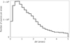 |
Fig. 1. Distribution of angular distance between Catalina CSS South targets and their Gaia candidate counterparts found within a radius of 5″. |
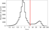 |
Fig. 2. Distribution of the synthetic distance of candidate counterparts obtained by the cross-match between Gaia and Catalina CSS South. An upper limit of ρsynth = 6 was applied to filter out mismatches. |
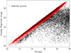 |
Fig. 3. Gaia magnitude vs. Catalina magnitude for candidates. The counterpart sources with ρsynth < 6 are plotted in red. |
Figure 2 shows the distribution of the ρsynth. The abscissa is in log-scale for clarity. This plot led to the selection of the cut-off value ρsynth = 6. The difference in photometric magnitudes between Gaia and Catalina is shown in Fig. 3, where the Gaia magnitude of the candidate Gaia matches is plotted on the horizontal axis and the corresponding Catalina magnitude is given on the vertical axis. The Gaia sources selected by the ρsynth < 6 constraint are shown in red, and ∼36 900 sources are left. The next step was to reduce any remaining multiple matches to a single match. In this example, fewer than 200 sources are multiple matches. We kept those with the lowest value of ρsynth. The final cross-matched catalogue for Catalina Surveys Southern periodic variable star catalogue contains 36 584 sources.
2.3. Assembly of the final catalogue
After cross-matching of all of the individual catalogues, we merged the per-catalogue results to form a single cross-match data set. It is expected that many of the input catalogues overlap, and some of these sources may appear in several input catalogues with different information of their name, variability type, or their variability period. In order to guide users towards the most likely class and period, we defined an approximate catalogue ranking list. This was not a perfect solution because catalogue classifications may be more accurate for some types of objects than others. Catalogues that did not overlap with others did not compete in the ranking, so that their relative position is not meaningful and could go to any place. Table A.2 shows the rank-ordered list of literature catalogues. The higher the place of a catalogue in the list, the more accurate the catalogue in general.
Source matches of multiple catalogues to the same Gaia source identifiers were merged. The resulting cross-match catalogue contains one Gaia source per row, together with information from all relevant catalogues, sorted according to their rank. For convenience, information from the highest ranked catalogue for a given source is replicated in single-element ‘primary’ fields (e.g., primary_var_type and primary_period, see Table A.4).
During the assembly of the catalogue, we tried to homogenise the labels of the variability classes used in the literature. The often different literature class labels for the same types were made homogeneous following the nomenclature used by the AAVSO4, except for a few exceptions (e.g., SARG, OSARG, GTTS, and IMTTS). Some type labels were relabelled ‘OMIT’ as primary class because they were too generic, uncertain, or with insufficient variability characterization, and thus should be omitted from training or completeness and purity estimates. The number of literature catalogues for eclipsing binaries is large, and different authors use different labels in their works. In order to homogenise the naming of eclipsing binaries, we grouped them into four subclasses: EA, EB, EW, and ECL, with the latter denoting the generic class when there is no further information or when the subclass is uncertain. Table A.3 shows the grouping of labels as defined in our catalogue. Information on the original labels from literature was preserved, however. As a special case, sources from the Gaia alerts5 have class labels set to OMIT if they were recorded after 28 May 2017 (Gaia DR3 observation time limit). There are 5676 such sources, and 49% of them were reported by Gaia alerts. The rest were also included in other input catalogues. In some catalogues, sources could be associated with multiple types, in which cases, OR as | and AND as + were used. We respected the source classification given in the original catalogues; therefore, class labels may refer to any level of a possible hierarchy. For example, a source may be classified as AGN, QSO, BLAZAR, or BLLAC, without implying that a subtype (e.g., BLLAC) does not belong to its superclass (e.g., BLAZAR or AGN).
After merging information of overlapping catalogues, the final cross-match catalogue contains 7 841 723 unique Gaia DR3 source ids. This represents 0.43% of the 1.8 billion sources available in DR3. The variability processing produced 9 976 881 variable stars (Rimoldini et al. 2023) and 2 451 364 galaxies (Gaia Collaboration 2023) through the classification pipeline. Of the variable stars, 2 308 354 are part of this cross-match catalogue, and it also contains 973 808 galaxies. A subset of catalogues with particularly low contamination rates is indicated by a boolean column selection and includes 6 697 530 sources. Sources with class ‘OMIT’ are filtered out from the selection. The properties of the final catalogue are discussed in the next section.
2.4. Caveats and exceptions in the pipeline
The method described above, using the statistics of each catalogue, has the advantage of automatically eliminating large numbers of outliers. It also provides a clean data set. However, as a statistical process, it may sometimes reject perfectly good candidates. For example, Gaia source_id 4040728046945051264 exists in both OGLE4_CEP_OGLE_2020 (Soszyński et al. 2020), as OGLE-BLG-T2CEP-0346, and COMP_VAR_VSX_2019 (Watson et al. 2006, VSX version 2019-11-12), with OID = 33239. The angular distance of this source with respect to its Gaia counterpart is Δθ = 0.89″in both catalogues (VSX includes OGLE stars). Figure 4 shows that for OGLE4_CEP_OGLE_2020, most of the counterpart sources exist within 0.3″, while in COMP_VAR_VSX_2019, which is a compilation of sources from various catalogues, it is close to 1″. Thus, due to different cuts, this source was eliminated from OGLE4_CEP_OGLE_2020, but not from COMP_VAR_VSX_2019.
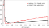 |
Fig. 4. Angular distance distribution (normalised to maximum) of Gaia cross-match candidates for OGLE4_CEP_OGLE_2020 and COMP_VAR_VSX_2019. |
The cross-match was purely astrometric (based only on the smallest Δθ) in the following special cases: catalogues with highly non-uniform photometry (bands, methods, etc.), whose distribution of ρsynth was not adequate to split matches from mismatches, catalogues whose photometry was biased by extreme variability (e.g., sampling only the peak brightness of cataclysmic variables), and very small catalogues for which a statistical procedure was not applicable.
Exceptionally, some catalogues that required no cross-match were included, such as DPAC internal catalogues with pre-assigned Gaia source_id and EROSITA_AGN_LIU_2021, for which the authors had already performed cross-match with Gaia in Salvato et al. (2022) using methods optimised for X-ray data sets. We therefore used their results.
3. Cross-match catalogue
In this section, a description of the catalogue and its general properties are discussed. It is published online through the website of the Centre de Données astronomiques de Strasbourg.
3.1. Description of the catalogue
The cross-match catalogue contains 7 841 723 sources of various types (6 697 530 of them are flagged as selection=true). Table A.4 shows the available fields in the published catalogue and provides a short description. Columns in plural may contain multiple values, separated by a semicolon, as a source may exist in several literature catalogues. Their order follows the ranking list. The fields starting with primary contain the information from the highest ranking catalogue in which a specific source exists. The primary_superclass field was introduced in order to group smaller classes and facilitate the selection of generic types. Table A.5 presents the available types in primary_superclass, the number of sources, and classes assigned to each superclass. The assignment was performed based on the class in the highest ranking catalogue, which is given in primary_var_type. var_types contains the homogenised variability class, original_var_types lists the original variability type from the literature (i.e. not homogenised), and original_alt_var_types shows any alternative variability types provided in literature. Despite our best effort at minimising mismatches, the cross-match catalogue may still associate sources with incorrect classifications because of remaining mismatched sources or inaccurate classifications in the literature. No cleaning or corrections were performed with respect to the information from the literature. Thus, depending on the purpose, users might need to verify or clean some objects of interest, especially when the selection flag is not used.
The final product contains 112 different types of objects. Some of them are not variable, like constants (CST), generic white dwarfs (WD), non-variable DQ dwarfs (DQ, HOT DQ, and WARM DQ), or galaxies that appear artificially as variable in Gaia (Holl et al. 2023), as they might be relevant (depending on the purpose) to distinguish genuine from spurious light variations. The full list of the 112 different types ordered alphabetically is presented in Table A.6, together with the number of objects: the first column shows the variability class, the following two columns present the number of objects of this type in primary_var_type, and the last two columns refer to the number of unique sources that were classified in any input catalogue as the specific class (in var_types).
3.2. Properties of the catalogue
The sky distributions of cross-match sources are presented in Figs. 5–7, where all sources, only variable stars (without WD, CST, AGN, and GALAXY types), and only constant sources are shown. The sky distributions for the extragalactic content are presented and discussed in Sect. 4.6. The Galactic centre, Magellanic Clouds, the Kepler fields, and the SDSS Stripe 82 are prominent as some literature catalogues are focused in those fields.
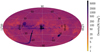 |
Fig. 5. Sky density of all sources in the cross-match catalogue. |
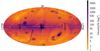 |
Fig. 6. Sky density of 3 157 191 variable stars in the cross-match catalogue. |
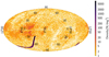 |
Fig. 7. Sky density of 688 960 constant sources in the cross-match catalogue. |
Figure 8 shows the distribution of magnitudes of all sources (black) and of constants (blue), variable objects (red), and galaxies (dashed green). The shape of the magnitude distributions represents the selection function of the literature catalogues used to form this cross-match. Fewer constant sources lie in the range 12 < G < 14 (see Sect. 2.1), however, which is visible, but is partially covered with the ZTF and TESS least variable sources identified in this work (Sect. 5). The galaxies appear at the fainter end of the catalogue, while variable and constant sources are distributed along the full magnitude range.
 (2)
(2)
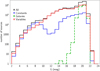 |
Fig. 8. Magnitude distribution of the cross-match catalogue for galaxies, variables, and constants. |
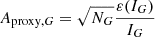
Figure 9 presents the values of an amplitude proxy in G (Aproxy, G; Mowlavi et al. 2021) versus the mean G-band magnitude for the variable stars and constant sources. The amplitude proxy is a measure of the scatter in the light curve of each source. Aproxy, G is defined in Eq. (2), where NG is the number of observations contributing to the G photometry, and IG and ε(IG) are the G-band mean flux and its error. A fraction of stars classified as variable in the literature have low Aproxy, G, sometimes lower than constant sources. An example is source_id 3328974248568180864, which has Aproxy, G = 0.0016 and is classified as an eclipsing binary with a period of 1.04 days by ASAS-SN (ASASSN − V J061917.53+094328.8). The ASAS−SN time series6 shows a few points in eclipse, which could justify the low value of the amplitude proxy, especially if Gaia missed measurements in eclipse. On the other hand, there is a number of ‘constant’ sources with large Aproxy, G. The extreme case of source_id 395015018457259904, Aproxy, G = 0.29 and mean magnitude G = 15.57 is identified as constant in this work with data from the ZTF. The time series from the ZTF (Fig. 10) shows a constant source with a few bright and faint outlying observations and more than 300 points with small dispersion, resulting in a low MAD value. When the four outlying points are removed, the standard deviation of the magnitude values is 0.016 mag. The large amplitude in the Gaia DR3 time series could be due to spurious measurements or transient events that were missed by the ZTF. The discrepant sources may need to be filtered out depending on the requirements of each used case. As an example, the Gaia DR3 paper on the classification of variables (Rimoldini et al. 2023) describes the cleaning process applied to these cross-match sources before they were used for training purposes.
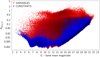 |
Fig. 9. Amplitude proxy G vs. mean G magnitude for constant and variable stars. |
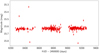 |
Fig. 10. ZTF time series of Gaia DR3 source_id 395015018457259904, which is selected as least variable, but has large Aproxy, G. |
4. Quality of the cross-matched sources
The following subsections assess the quality of the cross-matched sources per variability class. The assessment is based on a visual inspection of the variable source loci in the colour–absolute magnitude diagram (CaMD) with respect to a reference set defined with all the following criteria:
phot_g_mean_flux>0
phot_bp_mean_flux/phot_bp_mean_flux_error>10
phot_rp_mean_flux/phot_rp_mean_flux_error>10
phot_bp_n_obs>10
phot_rp_n_obs>10
parallax_over_error>10
visibility_periods_used>11
ruwe<1.2
These criteria were applied on all ∼1.8 billion Gaia DR3 sources. The outcome was further reduced by sampling on their parallax.
The result of this process was a set of 4.2 million sources with high astrometric and photometric quality. This reference set serves as background in the CaMDs that follow in order to help locate the areas the different variability types occupy.
Considering the significantly lower number of sources per class in the cross-match catalogue, less strict constraints were applied in order to select the sources of the various classes:
astrometric_excess_noise<0.5
parallax/parallax_error>5
visibility_periods_used>5
ruwe<1.4.
The sources within the Magellanic Clouds were excluded from the CaMDs. With these constraints, some rare types (e.g., black hole X-ray binaries (BHXB) and small amplitude red variables (SARV)) did not have sufficient representatives for the CaMD. In the following subsections, a short description of the properties of each class and discussion of the quality of the cross-match are given. More information about the various generic properties for each variability type can be found in the variable star-type designations of the AAVSO VSX7.
4.1. Pulsating variables
The cross-match catalogue contains many different classes of pulsating stars. Results are discussed separately for pulsating stars in dwarfs, sub-dwarfs, BLAPs, long-period variables, semi-regulars, Cepheids, δ Scuti, γ Doradus, RR Lyrae stars, and other types.
4.1.1. White dwarfs, sub-dwarfs, and blue large amplitude pulsators
There are ten different variability classes of variable white dwarfs (WD) and sub-dwarfs in the cross-match catalogue. Figure 11 shows the CaMD for these classes.
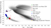 |
Fig. 11. CaMD of white dwarfs, sub-dwarf variables, and blue large amplitude pulsators. The sources of the reference data set are plotted in grey scale as background to facilitate locating the different areas. |
Several classes overlap or are different sub-classes of a larger class, such as the ZZ Ceti stars (for a detailed review of pulsating white dwarfs, see Córsico et al. 2019). Class labels are defined as described below.
– HOT_DQV: These sources are DQ white dwarf variables with C- and H-rich atmospheres. In the CaMD plot, the majority of the stars are clearly in the WD sequence below the area of V777 Herculis stars.
– ZZ_Ceti: For ZZ Ceti types, there are six subtypes in the catalogue, three of which concern ZZA (DAV). A few ZZ Ceti have no further subclassification.
– ZZ: These are generic ZZ Ceti without detailed class. They lie in the correct position in the CaMD.
– ZZA: ZZA (or DAV) are classical ZZ Ceti stars with DA spectral type with H atmospheres. They lie in the expected area in the CaMD of Fig. 11, but four ZZA appear to be well beyond the ZZ Ceti location. These sources originate from the VSX, which is very useful because of its diversity. Its cross-match is prone to mismatches, however.
– HOT_ZZA: The only HOT-ZZA that survived the quality cuts for the CaMD lies in the correct place with respect to ZZA and ZZB, as their effective temperature is in a similar range.
– ELM_ZZA: Extremely low mass (ELM) ZZA tend to have temperatures between 7800 and 10 000 K. The difference between ELM-ZZA and ZZA is clear. The ELM-ZZA on the right is SDSS J184037.78+642312.3. This was the first identified ELM-ZZA (Hermes et al. 2012).
– V777HER: The V777 Herculis (or ZZB, DBV) are stars with He-rich atmospheres. Their periods range between 100 and 1400 s (Bognár et al. 2014). They are well defined in the CaMD. They are grouped in the WD sequence between the warmer GWVIR and the cooler ZZA.
– GWVIR: GW Virginis (or ZZO, DOV, or PG1159) stars are a subtype of ZZ Ceti with absorption lines of HeII and CIV. They are the hottest known type of pulsating WD and pre-white dwarfs. The population in our catalogue is well defined. Some sources lie off the white dwarf sequence and closer to the horizontal branch.
– Subdwarfs: The cross-match catalogue contains two classes of subdwarf B stars: V361 Hya and V1093 Her. The two types are concentrated in the extreme horizontal branch, as expected. Some of them (mostly V361 Hya stars) can be redder than the main clump, but they follow the blue horizontal branch (BHB). Most of the V361 Hya stars are hotter (with effective temperatures of 28 000–35 000 K) than V1093 Her (23 000–30 000 K), so that the two populations are not distinct and overlap, as predicted by their temperature range (Heber 2016).
– BLAP: Blue large amplitude pulsators (BLAPs) have temperatures as hot as sub-dwarfs, but larger amplitudes (Pietrukowicz et al. 2017). In our catalogue, only two survived the astrometric cuts. They lie on the horizontal branch.
4.1.2. Long-period and semi-regular variables
The result of this work contains several classes of long-period variables. As for white dwarfs, several classes overlap or are subclasses of a generic class. Figures 12a and 12b present the CaMD for long-period and semi-regular variables, respectively.
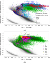 |
Fig. 12. CaMD of long-period (a) and semi-regular (b) variables. |
– LPV: Long-period variables include sources from surveys or catalogues that did not subclassify them.
They generally lie in the expected location in the CaMD, among the red giants. However, ∼3% of them are found on the main sequence. Half of them come from COMP_VAR_VSX_2019 and then from Gaia DR2 and CATALINA_VAR_DRAKE_2017. Additionally, 12 sources have literature periods shorter than one day, but only one of them has additional periods and is consistent with an LPV. For the rest, we tried to obtain additional information from the literature that it is not part of our work using the Vizier service. This effort revealed that 5 of them were identified as LPVs, providing periods consistent with the type, and one was identified as an eclipsing binary.
– M: M (or Mira, o Ceti) variables are late-type stars with periods between 80 and 1000 days. They are very well defined in the red part of the CaMD, with little contamination.
– M|SR: These are long-period variables that include Mira and semi-regular stars identified by classification in Gaia DR2 (Rimoldini et al. 2019a). The majority of this class occupies the expected area in the CaMD, overlapping the regions of Miras and LPVs. Some contaminants fall on the main sequence, however. These are likely young stellar objects (Mowlavi et al. 2018).
– SARG: These are small amplitude red giants pulsating with periods from 10 to 100 days. A large fraction of them have long secondary periods and lie on the RGB or AGB branches. Most of them are well defined in Fig. 12a, but a few are too blue or fall on the main sequence.
– OSARG: These are SARGs from OGLE. Their location on the red giant branch has very little contamination.
– LSP: Long secondary period variables are luminous red giants stars with a secondary period that is an order of magnitude longer than their primary period (Wood et al. 1999). One-third of the LPVs exhibit this type of behaviour (Soszyński 2007), and their periods range from 200 to 1500 days. In Fig. 12a they lie in a well-defined expected area that overlaps with other LPVs, although some outliers extend to the main sequence.
Semi-regular variables are in general giants or supergiants that exhibit irregular periods that vary. Some of them even show time lags of constancy. Figure 12b presents the CaMD for these classes.
– SR: Semi-regular variables are giants or supergiants of late type with no strict periodicity. Most of those that are on the main sequence are imported from ZTF_Periodic_Variables (Chen et al. 2020), likely due to misclassifications rather than mismatches, as several of them were verified to have the same periods in the Gaia counterparts.
– SRA and SRB: These are late-type giants and semi-regular variables. SRA stars tend to have periods of 35–1200 days, while the SRB stars are more irregular, with cycles of 20–2300 days, and also with time intervals that show no variability. These classes are well defined in the CaMD and have only few outliers, although they overlap with the other SR types. This is justified as typically, they all are of the same spectral type.
– SRC: This subclass consists of late-type supergiants with periods that fall into the interval of thirty to thousands of days. In the CaMD, they occupy a well-defined area above the SRA and SRB stars.
– SRD: These are giants and supergiants of types earlier than SRA, SRB, and SRC, with variability periods from 40 to 1100 days. In the CaMD, they are close to but separate from the other subclasses, towards earlier spectral types.
– SRS: These are red giants with shorter periods than other SRs. The periods vary from a few days up to a month. This class is defined in the same area as the other SR stars in the CaMD, but they appear to have several contaminants as well. All of the SRS stars originate from the VSX.
– PPN: These are protoplanetary nebulae with yellow supergiant post-AGB stars. Their variability resembles that of the SRD variables. The few that survived the quality cuts are found in reasonable places in the CaMD.
4.1.3. RR Lyrae stars
Many input catalogues contain RR Lyrae stars. This allows us to construct a significant sample of this type of variable stars and of its subclasses. They are A- to F-type stars showing a periodicity of less than a day and amplitudes that can reach two magnitudes in the optical. The RR Lyrae variables in the cross-match are divided into four subclasses and a generic class for the catalogues that do not provide detailed classification. Figure 13 shows that the majority of the sources falls into the expected place, but a significant fraction does not. Many sources are located in the lower part of the main sequence, and some are between the main and white dwarf sequences. Visual inspection shows that some of them were mismatched sources. When in dense regions, two Gaia sources may have a similar angular distance to the literature target and the most compatible magnitude associated with the incorrect counterpart. The user is encouraged to verify sources of these classes, especially if not filtering input catalogues.
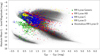 |
Fig. 13. CaMD of RR Lyrae stars. |
– RR: This is the generic class of RR Lyrae stars from catalogues that do not provide subclasses. The majority of those stars are from PS1_RRL_SESAR_2017 (Sesar et al. 2017), which contains several problematic cases of sources lying in the white dwarf sequence or between the white dwarf and the main sequence. This is expected because no selection based on score was applied to these candidates (unlike in PS1_RRL_SESAR_SELECTION_2017).
– RRAB: This is the most common RR Lyrae class, with asymmetric light curves in the optical wavelengths, where there is a quick rising phase followed by a slow decline of their brightness. Their periods vary between 0.3 and 1 day. The majority of them lie in the expected place in the CaMD, with a few outliers towards the white dwarf sequence.
– RRC: These have symmetric and sinusoidal light curves and shorter periods than RRAB stars. In the CaMD, they mostly have GBP − GRP ∼ 0.5 mag, but also extend to the main sequence.
– RRD: These are double-mode pulsators that occupy a well-defined region at GBP − GRP ∼ 0.5 mag, but there are also some very red outliers.
– ARRD: These are anomalous RRDs, double-mode pulsators that are similar to RRDs, but their period ratios are different. Very few ARRDs survived the quality cuts for the CaMD. They are scattered towards the red part of the main sequence.
4.1.4. Cepheids
In our catalogue, we included several types of Cepheids. The relevant CaMD is presented in Fig. 14.
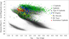 |
Fig. 14. CaMD of the different types of Cepheids. |
– CEP: Cepheids are radial pulsating giants and supergiants with a wide range of periodicities from ∼1 to more than 100 days. Their spectral type varies depending on their phase from F to K. This class label includes all types of Cepheids from catalogues that do not provide a detailed classification. Only a small number of sources of this class is included in the CaMD. Half of them lie in a reasonable location, and the other half falls on the main sequence.
– ACEP: Anomalous Cepheids, or BL Bootis, are pulsating variables that lie on the instability strip. They typically have periods from a few hours to two days. The ACEPs found in the CaMD occupy the expected position.
– DCEP: δ Cepheids, or classical Cepheids, tend to be brighter than the type II Cepheids. Some sources in the cross-match fall on the main sequence, however.
– T2CEP: This is a generic class of type II Cepheids from catalogues that do not provide further details about their subclass. They are pulsating variables with periods in the interval from 1 to more than 50 days. They are similar to classical Cepheids, but with lower masses and luminosities, and they tend to be older. They can be divided into three subclasses: BLHER, CW, and RV TAU. These subclasses have different period ranges, as shown in Fig. 15, while the generic class spreads throughout the full range of periods in the plot.
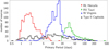 |
Fig. 15. Period distribution of type II Cepheids, as reported in the literature. The different colours show the three subclasses and the generic class. |
– BLHER: BL Herculis (or CWB) are the type II Cepheid variables with the shortest periods of the different subclasses. They have periods from one to four days, and they lie in the region between the horizontal branch and the asymptotic giant branch. Only 90 out of the 1153 BLHER in our catalogue survived after the quality cuts. Some of them are found to be redder than expected.
– CW: W Virginis stars have periods between 10 and 20 days. They cross the instability strip. They expand to the areas of BL Her and RV Tau in the CaMD. Their period distribution reported in the literature has tails that extend to the full range shown in Fig. 15.
– RV: RV Tauri variables are radially pulsating supergiants that change their spectral type along with their magnitude. Their spectral type spans from F–G class to K–M, depending on their phase. Their periods are longer than 30 days, with typical values between 40–50 days. The RV Tau stars in the cross-match catalogue fall into the expected CaMD location.
4.1.5. δ Scuti and γ Doradus variables
Because δ Scuti and γ Doradus variables are closely related and can also be hybrids, they are presented together in Fig. 16.
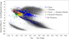 |
Fig. 16. CaMD of the different types of δ Scuti and γ Doradus stars. |
– DSCT: δ Scuti are pulsating variables similar to δ Cepheids. They follow the same period–luminosity relation, but they have shorter periods (from 0.01 to 0.2 days). Their brightness varies with amplitudes between 0.003 and 0.9 mag. Their spectral type is between A0 and F5. Usually, δ Scuti stars lie on the instability strip. Figure 16 shows several contaminants as the δ Scuti representatives cover a large fraction of the main sequence, with some sources on the white dwarf sequence.
– SXPHE: SX Phoenicis are considered similar to δ Scuti stars. But they are subdwarfs with periods typically in the lower part of the DSCT range. They lie in the expected place of the CaMD.
– DSCT|SXPHE: These are δ Scuti or SX Phoenicis stars identified by the classification of the variable sources of Gaia data release 2. They generally occupy a correct region, although there are some outliers.
– GDOR: γ Doradus stars are dwarfs with late-A to late-F spectral type that exhibit variability with non-radial pulsations. They usually have periods of about one day. In Fig. 16, they occupy the expected region, except for some outliers.
– DSCT+GDOR: The δ Scuti and γ Doradus hybrids are variable stars that exhibit both g-mode (GDOR) and p-mode (DSCT) pulsations. They are found in the expected location of the CaMD.
4.1.6. Other pulsating variables
Our cross-match catalogue contains other types of pulsating variable stars that don’t fit in the above groups. These additional pulsating types are presented in this subsection. Figure 17 presents the corresponding CaMD.
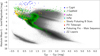 |
Fig. 17. CaMD of the other types of pulsating variable stars. |
– ACYG: α Cygni stars are B–A supergiants exhibiting non-radial pulsations with a wide range of periods. The typical amplitude of their photometric variability is about 0.1 mag. In Fig. 17, they may spread more than anticipated for A- or B-type stars.
– BCEP: β Cepheid stars are main-sequence stars of O8–B6 spectral type exhibiting photometric and radial velocity variability with short periods between 0.1 and 0.6 days. A large number of BCEP stars was cross-matched. The majority originates from KEPLER_VAR_DEBOSSCHER_2011, but no probability thresholds were applied. The vast majority are therefore misclassified sources, and none of those in the CaMD lies in the expected region. If the selection flag is not active, we encourage rejecting unfiltered BCEP stars with primary_var_type originating from KEPLER_VAR_DEBOSSCHER_2011 and also from ASAS_VAR_RICHARDS_2012, which fall on the RGB.
– SPB: These are slowly pulsating B stars that pulsate in high radial mode with periods from one to four days (Southworth et al. 2021) and amplitudes of up to 0.1 mag. Not all sources are compatible with the B-type colour (reddened or not) in Fig. 17. Contaminants lie lower on the main sequence or among the red giants.
– ROAP: Rapidly oscillating Ap stars are Ap/Fp stars that show photometric and radial velocity variability. Their period is shorter than 24 min (Balona 2022), and their amplitudes are lower than 0.01 mag. The ROAP stars identified in the cross-match occupy the expected area in the CaMD, as shown in Fig. 17.
– ROAM: Rapidly oscillating Am stars, like ROAPs, are chemically peculiar A stars, but their spectral type is Am. They oscillate with periods between 8 and 22 min, and have small amplitudes of up to 0.01 mag. They occupy a similar place in the CaMD next to the ROAPs.
– PVTEL: PV Telescopii are supergiants of several spectral types with a hydrogen deficiency. They are divided into thee subclasses of different period ranges, from 0.5 to 100 days. In the CaMD, they lie in the expected region, and their extended range of colours corresponds to the three subclasses. The hottest is of type II with the shortest periods, and the coolest stars are of type III and exhibit the longest periods in the range.
– ZZLEP: ZZ Leporis stars are central stars of planetary nebulae that exhibit photometric variations. They are O-type stars with periods that range from hours to days. The ZZ Lep stars in Fig. 17 are compatible with O-type stars, some of which are reddened.
– PULS-PMS: Pulsating pre-main-sequence stars are Herbig Ae/Be stars of B or A types that are in their PMS phase and have the right combination of physical parameters to become vibrationally unstable (Zwintz & Weiss 2006). In the CaMD of Fig. 17, half of them seem to have the expected colour.
4.2. Cataclysmic variables
A few types of cataclysmic variables are included in the cross-match. The most important ones are shown in Fig. 18 and are discussed in this section. As described in Sect. 2.4, due to the nature of cataclysmic variables, the synthetic distance was not used for catalogues of these objects (e.g., ZTF_CV_SZKODY_2020, SDSS_CV_SZKODY_2011) because the reported magnitude may refer to a measurement during the outburst phase. However, it maybe used when the identification of these objects came from a survey containing multiple classes (e.g., ASASSN_VAR_JAYASINGHE_2019).
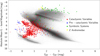 |
Fig. 18. CaMD of cataclysmic variable stars. |
– PCEB: Pre-cataclysmic variables or post-common envelope binaries are binaries of a white dwarf and a main-sequence star or a brown dwarf. In Fig. 18, most of them lie on the extreme horizontal branch.
– CV: This is the generic type of cataclysmic variables that includes novae and dwarf novae. They typically fall between the main sequence and the white dwarf sequence in the CaMD.
– ZAND: Z Andromedae stars include inhomogeneous types of symbiotic binary variable stars composed of a giant and a white dwarf. They display irregular variability with large amplitudes. Most of the few cases that are present in Fig. 18 lie on the AGB branch.
– SYST: These are symbiotic stars, which, like ZAND, form a heterogeneous group of objects, usually with a red giant or AGB star and a white dwarf. Most of them fall on the AGB branch in the CaMD.
4.3. Eclipsing binaries, double periodic variables, and stars with an exoplanet
The CaMD for the eclipsing binary stars and stars with exoplanets in the data set is presented in Fig. 19. As described in Sect. 2.3, we homogenised the various types of binaries in four major types (see Table A.3). The properties of these types are presented in this section. The eclipsing binaries can be scattered throughout the HR diagram, as shown in the figure. The generic class ECL is not plotted as it totally overlaps with the other classes on the main sequence.
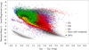 |
Fig. 19. CaMD of eclipsing binaries and stars with transiting planets. |
– EA: Algol-type (β Persei) eclipsing binaries have stars with spherical or only slightly elliptical shape. The secondary eclipse is not always present in the time series. Figure 19 clearly shows that this type of object can be anywhere in the CaMD.
– EB: β Lyrae eclipsing binaries have elliptical components. The secondary minimum is always visible in their light curve. The periods of most of these eclipsing binaries are longer than half a day. They usually cover the upper part of the main sequence and extend to the giants.
– EW: W UMa-type eclipsing binaries are composed of two stars of similar spectral type between A and K. Most of them are F or G. They have short periods, typically between 0.25 and 1 day. There are many red stars in Fig. 19, and ∼3% have periods longer than 2 days in the literature, ∼30% of which have different classifications (e.g., ROT or YSO) in other catalogues. The literature period distribution of this class is shown in Fig. 20, with a strong peak at about 0.37 days, but also with a tail extending to more than 200 days. The peak at 0.37 days for contact binaries was also observed by Paczyński et al. (2006), but more recent studies found that EW present different peaks with a maximum at 0.29 days (e.g., Qian et al. 2017).
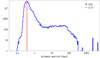 |
Fig. 20. Distribution of periods from the literature for EW-type eclipsing binaries. |
– DPV: Double periodic variables are semi-detached interacting eclipsing binaries that exhibit photometric variability with two distinct periods. Only three of them are shown in Fig. 19.
Although not a system of binary stars, stars with transiting exoplanets (EP) are added to Fig. 19, where they lie on the main sequence. About 48% of the exoplanets included in our catalogue have an original identification that belongs to Kepler (Kepler or K2), and another 11% come from the Kepler input lists (EPIC, KOI, and KIC). The majority of Kepler targets that come from the EPIC list have K-M spectral type (Huber et al. 2016), followed by those of F-G type. The colour of most EPs in Fig. 19 is BP − RP < 1.5.
4.4. Eruptive
The compilation of variables from the literature contains 18 eruptive variability types. Many of them are different subtypes of T Tauri stars (TTS), which are plotted in Fig. 21a separately from other eruptive types in Fig. 21b. Both plots contain stars that are fainter and bluer than the expected pre-main-sequence locus. This is likely due to the circumstellar discs of these stars at high inclination. The photosphere is therefore strongly extincted, and their optical colours are bluer due to the light scattered by the disc atmosphere. A short discussion of the properties of all available eruptive stars is given below.
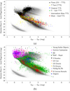 |
Fig. 21. CaMD of eruptive-type variable stars. Panel a shows the various TTS types and flare stars, and panel b shows the rest of the eruptive-type stars. |
– TTS: T Tauri is the generic class of pre-main-sequence objects. They are generally low- to intermediate-mass stars in a stage between protostars and low-mass main-sequence stars. In Fig. 21a, they occupy the expected region, but a small fraction is bluer than the main sequence or is falling on the main sequence. Most of these stars are in the Orion molecular cloud. There are several TTS subclasses in the cross-match catalogue, depending on their spectra (Herbst et al. 1994; Herbst & Shevchenko 1999).
– CTTS: Classical TTS are well-studied stars. They are young accreting stars in late stages of their evolution from protostars to the main sequence. They are well defined in Fig. 21a, although there are a few misplaced sources, half of which are part of the Orion molecular cloud.
– GTTS: G-type TTS are G- and K0-type TTS. Only a few GTTS are available, and they fall in the expected place in the CaMD.
– WTTS: Weak-lined or ‘naked’ TTS have little or even no accretion disc. They also follow the TTS trend in the CaMD, with a few exceptions.
– IMTTS: Intermediate-mass TTS have masses between 1 and 4 M⊙ and are considered precursors to the PMS Herbig Ae/Be stars (Lavail et al. 2017).
– Flares: This is a generic type, encapsulating several other types exhibiting flares due to magnetic activity (UV Ceti, TTS, etc.). In the CaMD, it is evident that they are spread throughout the main sequence and in the RGB.
– HAEBE: Herbig Ae/Be variables are young stars of spectral types A or B. There are only a few of them, but mostly in the expected location of the CaMD, including some very reddened ones.
– FUOR: FU Orionis variables are pre-main-sequence stars closely related to the evolutionary stages of T Tauri stars. They are characterised by rapid and strong photometric and spectral variability. Only three of the nine FUOR stars in the cross-match catalogue survived the quality cuts, and they are in reasonable places in the corresponding CaMD.
– UV: UV Ceti flare stars have spectral types K or M. Figure 21b shows many stars spread in the main sequence up to earlier spectral types.
– GCAS: γ Cassiopeiae stars are of O9–A0 type and thus occupy the expected place in the CaMD. Some are of later types, but without obvious problems. Some of them have been assigned different types in other input catalogues (e.g. some of those on the extreme horizontal branch are also classified as CV).
– BE: These are B-type emission line variables that might be γ Cas stars or λ Eri. The cross-match catalogue includes many misclassified objects in the lower part of the main sequence.
– UXOR: UX Orionis stars are a subclass of Herbig Ae/Be stars, consistent with their location in the CaMD.
– RCB: R Coronae Borealis stars can have several diverse spectral types. In this work, a large fraction of them are post-AGB stars that exhibit RCB variations, but they share the same origin.
– SDOR: S Doradus stars (or luminous blue variables) are evolved stars characterised by large amplitude variations of Bpec to Fpec spectral type, as confirmed by their position in the CaMD.
– YSO: These are young stellar objects of the generic type; many of them are TTS. The majority of them lie on the TTS region, but others are scattered all around.
– I: These are irregular stars that are mostly YSOs, which is confirmed by their distribution in the CaMD.
– DIP: Dippers are pre-main-sequence stars of K and M spectral type and exhibit dips in their light curves. They lack a strict periodicity. The few dippers presented in Fig. 21b are in the expected colour range of this type of stars.
– WR: The Wolf-Rayet stars are a group of massive stars that present broad emission lines. They have high temperatures and luminosities and are considered as descendants of O-type stars. Their variability is not periodic. In the CaMD, a few WR stars lie in the expected area, and others appear to be reddened.
4.5. Rotational
Rotational variables are stars whose variability is caused by their rotation and asymmetries in shape or non-uniform surface brightness. The cross-match catalogue contains 13 types of rotational variables (some of them overlap), and their CaMD is shown in Fig. 22.
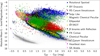 |
Fig. 22. CaMD of the rotational types of variable stars. |
– ROT: This is a generic class of spotted stars. They are scattered throughout in the CaMD.
– RS: RS Canum Venaticorum variables are close binary systems of late spectral type that exhibit chromospheric activity. As shown in Fig. 22, they extend throughout the main sequence, and many of them are very red. The vast majority of these sources originates from the automatic classification of ZTF_PERIODIC_CHEN 2020.
– ACV: α2 Canum Venaticorum variables are chemical peculiar main-sequence stars of B8p–A7p type with strong magnetic fields. Their periods vary from 0.5 to more than 100 days. Most of the ACV stars fall into the expected region of the CaMD, with a few red outliers. A large fraction of these outliers are listed in the VSX and originate from Kabath et al. (2009).
– SXARI: SX Arietis are B-type chemical peculiar stars with strong magnetic fields and periods of about one day. They are similar to ACV stars, but have higher temperatures. Therefore, their distribution in the CaMD overlaps to some extent. Our list includes a few SXARI stars whose period is much longer than one day, and thus their class is spurious.
– MCP: These are magnetic chemically peculiar stars that include Ap, HgMn, and Am types. They naturally overlap with ACV and SXARI variables (and many of them are classified as ACV in other catalogues).
– CP: This is a generic class of chemically peculiar variables originating from Richards et al. (2012), which were selected using a random forest classifier. The class includes mostly hot stars, but also few cooler stars of G and later spectral type, with GBP − GRP > 1.5.
– FKCOM: FK Comae Berenices variables are G to K giants that rotate rapidly and have strong magnetic fields. Only a few FKCOM variables exist in the cross-match catalogue, but they have the expected colour and absolute magnitude for their type.
– BY: BY Draconis stars are dwarfs that have inhomogeneous surface brightness and exhibit chromospheric activity. They have a periodic variability with periods that can vary from less than a day to more than 120 days. The cross-match catalogue has a large number of BY variables that fall on the main sequence, but a significant fraction of them has been classified into other classes as well.
– ELL: Ellipsoidal variables are close binaries whose light curves do not contain an eclipse, but their variability is due to the distortion of their shape from the mutual gravitational fields. The observed light therefore varies because the projected surface towards the observer varies. The sample of ellipsoidal variables is scattered throughout the CaMD, and the majority lies on the main sequence.
– HB: Heartbeat variables are binary star systems with eccentric orbits that cause both variations of stellar shapes and vibrations induced by these changes. There are about 150 heartbeat stars in the cross-match catalogue, 91% of which are also classified as eclipsing binary in various catalogues. The majority of those that passed the quality cuts for the CaMD have a colour of 0.1 < GBP − GRP < 1.0 mag. Only a few of them are redder than this.
– SOLAR_LIKE: These stars exhibit chromospheric activity and include BY, ROT, and Flare types. In the CaMD, most representatives fall on the main sequence, although there are other sources in the red giant branch.
– R: These are close binaries that exhibit strong reflection in their light curves (re-radiation of light of the hotter star from the surface of the cooler one). Most of these stars fall in the region between the main sequence and the white dwarfs; some are found on the extreme horizontal branch as well.
– BY|ROT: These are similar to SOLAR_LIKE and include stars of types BY or ROT, as defined before.
4.6. Extragalactic content
A large number of sources in the cross-match catalogue are galaxies and active galactic nuclei. Most of the input catalogues we used to cross-match galaxies and AGN were internal Gaia catalogues, and their content could be identified by their source_id. The catalogues containing AGN had various levels of detail in their classification (AGN, BLAZAR, BLLAC, and QSO), although most sources were grouped as QSO as a generic class. No subclasses were reported for galaxies. Figures 23a and 23b show the sky distribution of all types of quasars and galaxies. Darker colours indicate a higher density of the objects. Both figures show that the Galactic plane is avoided. As the main contributions for both galaxies and quasars are from Gaia products, their properties are discussed in detail in their corresponding papers (Krone-Martins et al. 2022; Gaia Collaboration 2022).
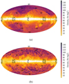 |
Fig. 23. Sky map of (a) 1 801 094 active galactic nuclei, blazars, and quasars in general, and (b) for the 1 746 224 galaxies. |
4.7. Class overlaps
Because so many catalogues contributed to this cross-match, different classes might be associated with the same sources. Table A.8 (available at the CDS) lists the sources that overlap based on their superclasses, ordered alphabetically. The first column shows the primary_superclass, and the 51 columns that follow list the overlapping superclasses taken from var_types. Not to be confused with the same classes, the numbers of sources that are classified as the same type in different catalogues (i.e., the diagonal of the table) were set to zero. We list below some of the reasons that lead to class overlaps.
– Mismatches: Due to the statistical approach used and the fact that each catalogue was treated separately, it is possible that Gaia sources are erroneously assigned to input catalogue counterparts. This problem may occur more frequently in crowded regions and also depends on the astrometric accuracy of each catalogue.
– Misclassifications: Input catalogues might include misclassified sources, especially when generated by automatic methods. An example is presented in Table A.7 for Gaia DR3 source_id 4066039874096072576, which is matched in four catalogues. This table lists the input catalogues, the identifiers of the source in each catalogue (with additional online information, if present), the coordinates, variability types, and periods. ASAS-SN classified this source as a semi-regular (with a classification probability of 0.537) and identified a variability period of ∼18 days. However, the other catalogues classified it as an eclipsing binary (EW, EB, and ECL) with a period of ∼2 days. The ASAS-SN database8 was used to download the photometric data of the source. Running a Lomb–Scargle (Lomb 1976; Scargle 1982) period search (using the R implementation of the lomb package; Ruf 2019) for each camera separately, we found that the periods were consistent with each other, and after doubling them (as is often needed for eclipsing binaries because they have two minima per cycle instead of only one, as targeted by the sine function in this period search method; see Fig. 1 of Holl et al. 2014), they corresponded to the 2.1091-day period identified in the other catalogues (see Fig. 24a). This source is also published in Gaia DR3 as an eclipsing binary with the same period. The period provided from ASAS-SN was recovered as a secondary peak in the frequencygramme, but the folded light curve was worse, suggesting that the correct type is EW rather than SR.
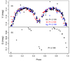 |
Fig. 24. Folded light curve for Gaia DR3 4066039874096072576 using different colours for each ASAS-SN camera. (a) The recovered period is almost always the same at 1.0545 days in the 3 different cameras provided by ASAS-SN, which is half of the period referred to in the literature. The folded light curve is plotted with twice the period recovered in each camera. (b) The same source using data and the period found in Gaia DR3. |
– Multiple classes: Some classes do not exclude others, and sources might be identified in the literature as a combination of two (or more) classes, such as Cepheids in eclipsing binaries or BY Draconis stars with flares of UV Ceti variables.
Table A.8 shows that the most strongly overlapped class is ECL as primary_superclass with RR Lyrae stars with 58 811 cases. However, the overlap rate is low because the cross-match catalogue contains more than 1.1 million sources whose primary_superclass is ECL. The catalogue_labels of these ∼59 K sources reveal that 56 361 of these are in PS1_RRL_SESAR_2017. This catalogue contains sources without filtering on the class probability. The high probability sources of this catalogue are provided in PS1_RRL_SESAR_SELECTION_2017, and only 1553 cases overlap with ECL. Moreover, the shapes of the light curves of EW and RRC stars are very similar and prone to confusion (Hoffman et al. 2009). Of the 1553 overlapped sources in PS1_RRL_SESAR_SELECTION_2017, 1162 are classified as RRC and EW.
Another significant overlap occurs between AGN and CST sources, of which 19 434 cases exist. In this case, the main contributor is GAIA_WD_GENTILEFUSILLO_2019 with 18 001 sources, while the rest are from SDSS_CST_IVEZIC_2007. In the first catalogue, no filtering was applied. When only the reliable sources were selected, (see Gentile Fusillo et al. 2019), 441 sources overlap. The overlap rate is very low because the primary_superclass of ∼1.8 million sources is AGN.
5. Selection of the least variable sources in the ZTF and TESS
5.1. Least variable sources in the ZTF
In order to increase the number of constant stars and widen their sky distribution, it was decided to take advantage of the wealth of the ZTF. The ZTF was started in 2017 at the Palomar observatory. Its goal is to provide a high-cadence data stream, enhancing science in stellar astrophysics, supernovae, active galactic nuclei, and so on. Each image is captured by a 47 square degree field camera mounted on the 48-inch Schmidt telescope. On average, the ZTF observes the entire northern sky more than 300 times per year (see Fig. 25) and issues a data release every two months. ZTF data release 2 9 has become available in December 2019 and contains ∼2.3 billion light curves.
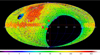 |
Fig. 25. ZTF r filter sky depth-of-coverage in Galactic coordinates. The colour scale corresponds to the number of observation epochs per approximate CCD-quadrant footprint. Image from the ZTF DR29. |
The idea was to obtain the ZTF photometric data and any statistic that is available in order to detect the least variable stars. However, there is no need to download all sources from the ZTF database as the aim is not a comprehensive detection of constant sources in ZTF. For this reason, a dense grid of points scattered throughout the ZTF observable sky was created, and ZTF sources were extracted by performing a cone search with a radius of 2′. The grid contained 36 000 points limited to δ > −30°, and it was created by obtaining healpix with depth 6 and nside 64.
In total, about three million ZTF sources were extracted. For all these sources, the median absolute deviation of their photometric time series was already available and was used to select the least variable stars. The three-million-source sample was divided into 250 magnitude bins, and the sources with MAD under the tenth, fith, and first percentile of the MAD distribution of each bin were selected. Figure 26 shows the ZTF median g magnitude versus time-series MAD. The sources with a MAD higher than the tenth percentile per magnitude bin are shown in grey, those with MAD between the tenth and fifth and the fifth and first percentiles are shown in red and blue, respectively, and sources with MAD lower than the first percentile are in green. Figure 27 shows the spatial distribution of the selected sources per percentile.
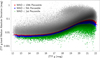 |
Fig. 26. MAD vs. magnitude per percentile cut for the ZTF sources in this work. Sources between the tenth and fifth percentiles are plotted in red, those with a MAD between the fifth and first percentiles are shown in blue, and those below the first percentile are presented as green crosses. |
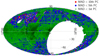 |
Fig. 27. Sky map of the least variable sources. The same colour-coding as in Fig. 26 for percentile (pc) thresholds has been used. |
The next step was to cross-match the selected sources with the Gaia DR3 data set, which was performed with the same method as for the rest of the catalogues in this document. At the end of this cross-match process, 267 784, 133 112, and 26 217 sources for the three different cut-offs (tenth, fifth, and first percentiles) were left. Figure 28 shows the G magnitude distribution of these sources depending on their corresponding percentile range. Because only very few sources lie at the bright end, it was decided to select an upper limit for the number of stars per bin (for a fairer representation of all magnitudes). Figure 29 shows the MAD vs. G magnitude of the selected stars (depicted in red), with a MAD lower than the tenth percentile and including up to 2000 sources per 0.5 mag bin. Figure 30 shows the G magnitude distribution of the final selection of sources.
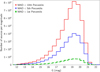 |
Fig. 28. Gaia G magnitude distribution of the selected least variable sources per percentile threshold after cross-match with Gaia DR3 data. The colour schema is the same as in Fig. 26. The line for MAD below the first percentile is dashed. |
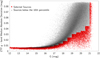 |
Fig. 29. MAD vs. G magnitude of sources below the tenth percentile of the MAD distribution. We highlight the sources that we selected as least variables in red. |
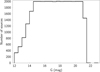 |
Fig. 30. G magnitude distribution of the final selection of sources with a photometric MAD below the tenth percentile, which highlights the ZTF cross-match representation as a function of magnitude. |
5.2. Selection of least variable sources from TESS
TESS is a NASA space telescope with the primary goal of searching for exoplanets. It observes both hemispheres divided into 26 sectors, and its targets are bright stars, most of which are brighter than T ∼ 12 mag. The TESS bandpass expands in the range from ∼600 to 1000 nm and is centred at the IC band (Sullivan et al. 2015). In order to overcome the lack of constant sources with magnitude around G ∼ 12 and considering the targets TESS observes, it was decided to apply the same process as described in Sect. 5.1 to TESS sources. The time series of ∼99 000 unique stars covering 11 sectors were used (see Fig. 31). We recall that our aim was not to cross-match the full TESS targets, but to identify a sufficient number of least variable stars in a specific magnitude range. The light curves were downloaded from the TESS bulk download website10, where a script is provided that extracts data per sector. About half of the sources were duplicated from sector overlaps at the ecliptic poles, and thus they were removed.
 |
Fig. 31. Sky coverage in ecliptic coordinates of the TESS sectors that were used in this work. |
These photometric time series contained the simple aperture photometry (SAP) and the pre-search data-conditioned simple-aperture photometry (PDCSAP) corrected flux of each object. The SAP flux is the raw flux, and from the PDCSAP flux, long-term trends were removed. This removal must be taken with caution as it can alter the true flux changes of variable sources. Fluxes were converted into magnitudes using a preliminary zero-point magnitude (László Molnár, priv. comm.), and the MAD was calculated for each source. The same procedure as in Sect. 5.1 was followed in order to select the sources with a lower MAD per magnitude bin. Figure 32 shows the MAD per magnitude per sector, revealing that sectors can have different MAD thresholds. The 10% least variable stars were therefore selected per sector. Figure 33 shows the final spacial distribution of the least variable stars in TESS. After the cross-matching with Gaia, 5100 sources were selected. The magnitude distribution of the selected sources is shown in Fig. 34, and it covers the magnitude gap of non-variable objects from HIPPARCOS and SDSS Stripe 82.
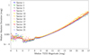 |
Fig. 32. TESS magnitude vs. MAD thresholds (of the tenth percentile) for the various sectors used. |
 |
Fig. 33. Least variable stars (green), the 10% we selected, plotted for the whole sample of TESS targets (blue). |
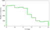 |
Fig. 34. Gaia G magnitude distribution of the 10% least variable stars in TESS after cross-matching with Gaia sources. |
6. Conclusions
We presented the creation of a large and diverse cross-match catalogue with Gaia from variable and constant sources in the literature. In total, 152 different input catalogues from the literature were cross-matched with Gaia DR3 in order to find the counterpart sources. This way, we compiled a large data set of more than 7.8 million sources and 112 different types of variables, constants, and galaxies. Each input was cross-matched individually by performing an epoch propagation and using a synthetic distance that encapsulates the astrometric distance and the photometric difference between targets and counterparts. The catalogue is available online to the scientific community through the website of the Centre de Données astronomiques de Strasbourg. Users of this catalogue might still need to verify or filter out some objects of interest, depending on the purpose of the analysis. This catalogue is a valuable resource for the studies of variable sources as it provides a single data set for the Gaia mission containing uniform photometry and astrometry.
Acknowledgments
We thank the referee Roberto Saito for his comments. This work has made use of data from the European Space Agency (ESA) mission Gaia (https://www.cosmos.esa.int/gaia), processed by the Gaia Data Processing and Analysis Consortium (DPAC, https://www.cosmos.esa.int/web/gaia/dpac/consortium). Funding for the DPAC has been provided by national institutions, in particular the institutions participating in the Gaia Multilateral Agreement which include, for Switzerland, the Swiss State Secretariat for Education, Research and Innovation through the Activités Nationales Complémentaires (ANC). This research has made use of the VizieR catalogue access tool, CDS, Strasbourg, France. We acknowledge with thanks the variable star observations from the AAVSO International Database contributed by observers worldwide and used in this research. Based on observations obtained with the Samuel Oschin 48-inch Telescope at the Palomar Observatory as part of the Zwicky Transient Facility project. ZTF is supported by the National Science Foundation under Grant No. AST-1440341 and a collaboration including Caltech, IPAC, the Weizmann Institute for Science, the Oskar Klein Center at Stockholm University, the University of Maryland, the University of Washington, Deutsches Elektronen-Synchrotron and Humboldt University, Los Alamos National Laboratories, the TANGO Consortium of Taiwan, the University of Wisconsin at Milwaukee, and Lawrence Berkeley National Laboratories. Operations are conducted by COO, IPAC, and UW. This paper includes data collected by the TESS mission. Funding for the TESS mission is provided by the NASA’s Science Mission Directorate. This work made use of software from Postgres-XL (https://www.postgres-xl.org), Java (https://www.oracle.com/java/), Q3C (Koposov & Bartunov 2006) and TOPCAT/STILTS (Taylor 2005).
References
- Abbas, M. A., Grebel, E. K., Martin, N. F., et al. 2014, MNRAS, 441, 1230 [Google Scholar]
- Akras, S., Guzman-Ramirez, L., Leal-Ferreira, M. L., & Ramos-Larios, G. 2019, ApJS, 240, 21 [NASA ADS] [CrossRef] [Google Scholar]
- Alfonso-Garzón, J., Domingo, A., Mas-Hesse, J. M., & Giménez, A. 2012, A&A, 548, A79 [NASA ADS] [CrossRef] [EDP Sciences] [Google Scholar]
- Baade, W. 1926, Astron. Nachr., 228, 359 [NASA ADS] [CrossRef] [Google Scholar]
- Balona, L. A. 2022, MNRAS, 510, 5743 [NASA ADS] [CrossRef] [Google Scholar]
- Beauchamp, A., Wesemael, F., Bergeron, P., et al. 1999, ApJ, 516, 887 [NASA ADS] [CrossRef] [Google Scholar]
- Belczyński, K., Mikołajewska, J., Munari, U., Ivison, R. J., & Friedjung, M. 2000, A&AS, 146, 407 [NASA ADS] [CrossRef] [EDP Sciences] [Google Scholar]
- Benkő, J. M., Bakos, G. Á., & Nuspl, J. 2006, MNRAS, 372, 1657 [CrossRef] [Google Scholar]
- Bergeat, J., Knapik, A., & Rutily, B. 2001, A&A, 369, 178 [NASA ADS] [CrossRef] [EDP Sciences] [Google Scholar]
- Bernhard, K., Hümmerich, S., Otero, S., & Paunzen, E. 2015, A&A, 581, A138 [NASA ADS] [CrossRef] [EDP Sciences] [Google Scholar]
- Boettcher, E., Willman, B., Fadely, R., et al. 2013, AJ, 146, 94 [NASA ADS] [CrossRef] [Google Scholar]
- Bognár, Z., Paparó, M., Córsico, A. H., Kepler, S. O., & Győrffy, Á. 2014, A&A, 570, A116 [NASA ADS] [CrossRef] [EDP Sciences] [Google Scholar]
- Bognár, Z., Kawaler, S. D., Bell, K. J., et al. 2020, A&A, 638, A82 [NASA ADS] [CrossRef] [EDP Sciences] [Google Scholar]
- Boller, T., Schmitt, J. H. M. M., Buchner, J., et al. 2022, A&A, 661, A8 [NASA ADS] [CrossRef] [EDP Sciences] [Google Scholar]
- Bonato, M., Liuzzo, E., Giannetti, A., et al. 2018, MNRAS, 478, 1512 [NASA ADS] [CrossRef] [Google Scholar]
- Bopp, B. W., & Stencel, R. E. 1981, ApJ, 247, L131 [NASA ADS] [CrossRef] [Google Scholar]
- Bradley, P. A., Guzik, J. A., Miles, L. F., et al. 2015, AJ, 149, 68 [CrossRef] [Google Scholar]
- Braga, V. F., Stetson, P. B., Bono, G., et al. 2016, AJ, 152, 170 [Google Scholar]
- Braga, V. F., Contreras Ramos, R., Minniti, D., et al. 2019, A&A, 625, A151 [NASA ADS] [CrossRef] [EDP Sciences] [Google Scholar]
- Bredall, J. W., Shappee, B. J., Gaidos, E., et al. 2020, MNRAS, 496, 3257 [NASA ADS] [CrossRef] [Google Scholar]
- Chang, S. W., Byun, Y. I., & Hartman, J. D. 2015, ApJ, 814, 35 [NASA ADS] [CrossRef] [Google Scholar]
- Chang, Y. L., Arsioli, B., Giommi, P., & Padovani, P. 2017, A&A, 598, A17 [NASA ADS] [CrossRef] [EDP Sciences] [Google Scholar]
- Chen, X., Wang, S., Deng, L., et al. 2020, ApJS, 249, 18 [NASA ADS] [CrossRef] [Google Scholar]
- Clementini, G., Ripepi, V., Leccia, S., et al. 2016, A&A, 595, A133 [NASA ADS] [CrossRef] [EDP Sciences] [Google Scholar]
- Clementini, G., Ripepi, V., Molinaro, R., et al. 2019, A&A, 622, A60 [NASA ADS] [CrossRef] [EDP Sciences] [Google Scholar]
- Corral-Santana, J. M., Casares, J., Muñoz-Darias, T., et al. 2016, A&A, 587, A61 [NASA ADS] [CrossRef] [EDP Sciences] [Google Scholar]
- Córsico, A. H., Althaus, L. G., Miller Bertolami, M. M., & Kepler, S. O. 2019, A&A Rev., 27, 7 [Google Scholar]
- Corwin, T. M., Sumerel, A. N., Pritzl, B. J., et al. 2006, AJ, 132, 1014 [NASA ADS] [CrossRef] [Google Scholar]
- Corwin, T. M., Borissova, J., Stetson, P. B., et al. 2008, AJ, 135, 1459 [Google Scholar]
- Cunha, M. S., Antoci, V., Holdsworth, D. L., et al. 2019, MNRAS, 487, 3523 [NASA ADS] [CrossRef] [Google Scholar]
- Dall’Ora, M., Clementini, G., Kinemuchi, K., et al. 2006, ApJ, 653, L109 [CrossRef] [Google Scholar]
- Dall’Ora, M., Kinemuchi, K., Ripepi, V., et al. 2012, ApJ, 752, 42 [CrossRef] [Google Scholar]
- De Medeiros, J. R., Ferreira Lopes, C. E., Leão, I. C., et al. 2013, A&A, 555, A63 [NASA ADS] [CrossRef] [EDP Sciences] [Google Scholar]
- de Vaucouleurs, G. 1978, ApJ, 223, 351 [NASA ADS] [CrossRef] [Google Scholar]
- Debosscher, J., Sarro, L. M., Aerts, C., et al. 2007, A&A, 475, 1159 [NASA ADS] [CrossRef] [EDP Sciences] [Google Scholar]
- Debosscher, J., Blomme, J., Aerts, C., & De Ridder, J. 2011, A&A, 529, A89 [NASA ADS] [CrossRef] [EDP Sciences] [Google Scholar]
- Demers, S., & Battinelli, P. 2007, A&A, 473, 143 [NASA ADS] [CrossRef] [EDP Sciences] [Google Scholar]
- Devor, J., Charbonneau, D., O’Donovan, F. T., Mandushev, G., & Torres, G. 2008, AJ, 135, 850 [Google Scholar]
- Drake, A. J. 2006, AJ, 131, 1044 [Google Scholar]
- Drake, A. J., Catelan, M., Djorgovski, S. G., et al. 2013a, ApJ, 763, 32 [NASA ADS] [CrossRef] [Google Scholar]
- Drake, A. J., Catelan, M., Djorgovski, S. G., et al. 2013b, ApJ, 765, 154 [Google Scholar]
- Drake, A. J., Gänsicke, B. T., Djorgovski, S. G., et al. 2014a, MNRAS, 441, 1186 [NASA ADS] [CrossRef] [Google Scholar]
- Drake, A. J., Graham, M. J., Djorgovski, S. G., et al. 2014b, ApJS, 213, 9 [Google Scholar]
- Drake, A. J., Djorgovski, S. G., Catelan, M., et al. 2017, MNRAS, 469, 3688 [NASA ADS] [CrossRef] [Google Scholar]
- Dufour, P., Béland, S., Fontaine, G., Chayer, P., & Bergeron, P. 2011, ApJ, 733, L19 [NASA ADS] [CrossRef] [Google Scholar]
- Dunlap, B. H., Barlow, B. N., & Clemens, J. C. 2010, ApJ, 720, L159 [CrossRef] [Google Scholar]
- Eker, Z., Ak, N. F., Bilir, S., et al. 2008, MNRAS, 389, 1722 [NASA ADS] [CrossRef] [Google Scholar]
- ESA 1997, in The HIPPARCOS and TYCHO Catalogues. Astrometric and Photometric Star Catalogues Derived from the ESA HIPPARCOS Space Astrometry Mission, ESA Spec. Publ., 1200 [Google Scholar]
- Eyer, L., Mowlavi, N., Evans, D. W., et al. 2017, ArXiv e-prints [arXiv:1702.03295] [Google Scholar]
- Eyer, L., Rimoldini, L., Rohrbasser, L., et al. 2020, in Stars and their Variability Observed from Space, eds. C. Neiner, W. W. Weiss, D. Baade, R. E. Griffin, C. C. Lovekin, & A. F. J. Moffat, 11 [Google Scholar]
- Eyer, L., Audard, M., Holl, B., et al. 2023, A&A, 674, A13 (Gaia DR3 SI) [NASA ADS] [CrossRef] [EDP Sciences] [Google Scholar]
- Flesch, E. W. 2015, PASA, 32, e010 [Google Scholar]
- Flesch, E. W. 2019, ArXiv e-prints [arXiv:1912.05614] [Google Scholar]
- Gaia Collaboration (Klioner, S. A., et al.) 2022, A&A, 667, A148 [NASA ADS] [CrossRef] [EDP Sciences] [Google Scholar]
- Gaia Collaboration (Bailer-Jones, C. A. L., et al.) 2023, A&A, 674, A41 (Gaia DR3 SI) [NASA ADS] [CrossRef] [EDP Sciences] [Google Scholar]
- Garofalo, A., Cusano, F., Clementini, G., et al. 2013, ApJ, 767, 62 [NASA ADS] [CrossRef] [Google Scholar]
- Gentile Fusillo, N. P., Tremblay, P.-E., Gänsicke, B. T., et al. 2019, MNRAS, 482, 4570 [Google Scholar]
- Gianninas, A., Bergeron, P., & Fontaine, G. 2005, ApJ, 631, 1100 [NASA ADS] [CrossRef] [Google Scholar]
- Graham, M. J., Kulkarni, S. R., Bellm, E. C., et al. 2019, PASP, 131, 078001 [Google Scholar]
- Hamanowicz, A., Pietrukowicz, P., Udalski, A., et al. 2016, Acta Astron., 66, 197 [NASA ADS] [Google Scholar]
- Hartman, J. D., Bakos, G. Á., Kovács, G., & Noyes, R. W. 2010, MNRAS, 408, 475 [Google Scholar]
- Heber, U. 2016, PASP, 128, 082001 [Google Scholar]
- Heinze, A. N., Tonry, J. L., Denneau, L., et al. 2018, AJ, 156, 241 [Google Scholar]
- Herbst, W., & Shevchenko, V. S. 1999, AJ, 118, 1043 [Google Scholar]
- Herbst, W., Herbst, D. K., Grossman, E. J., & Weinstein, D. 1994, AJ, 108, 1906 [Google Scholar]
- Hermes, J. J., Montgomery, M. H., Winget, D. E., et al. 2012, ApJ, 750, L28 [Google Scholar]
- Hermes, J. J., Montgomery, M. H., Gianninas, A., et al. 2013a, MNRAS, 436, 3573 [Google Scholar]
- Hermes, J. J., Montgomery, M. H., Winget, D. E., et al. 2013b, ApJ, 765, 102 [Google Scholar]
- Hey, D. R., Holdsworth, D. L., Bedding, T. R., et al. 2019, MNRAS, 488, 18 [NASA ADS] [CrossRef] [Google Scholar]
- Hoffman, D. I., Harrison, T. E., & McNamara, B. J. 2009, AJ, 138, 466 [NASA ADS] [CrossRef] [Google Scholar]
- Holl, B., Mowlavi, N., Lecoeur-Taïbi, I., et al. 2014, EAS Publ. Ser., 67–68, 299 [CrossRef] [EDP Sciences] [Google Scholar]
- Holl, B., Audard, M., Nienartowicz, K., et al. 2018, A&A, 618, A30 [NASA ADS] [CrossRef] [EDP Sciences] [Google Scholar]
- Holl, B., Fabricius, C., Portell, J., et al. 2023, A&A, 674, A25 (Gaia DR3 SI) [NASA ADS] [CrossRef] [EDP Sciences] [Google Scholar]
- Howell, S. B., Mason, E., Boyd, P., Smith, K. L., & Gelino, D. M. 2016, ApJ, 831, 27 [NASA ADS] [CrossRef] [Google Scholar]
- Hubble, E. P. 1926, ApJ, 64, 321 [Google Scholar]
- Huber, D., Bryson, S. T., Haas, M. R., et al. 2016, ApJS, 224, 2 [Google Scholar]
- Hümmerich, S., Mikulášek, Z., Paunzen, E., et al. 2018, A&A, 619, A98 [NASA ADS] [CrossRef] [EDP Sciences] [Google Scholar]
- Ivezić, Ž., Smith, J. A., Miknaitis, G., et al. 2007, AJ, 134, 973 [Google Scholar]
- Jayasinghe, T., Kochanek, C. S., Stanek, K. Z., et al. 2018, MNRAS, 477, 3145 [Google Scholar]
- Jayasinghe, T., Stanek, K. Z., Kochanek, C. S., et al. 2019a, MNRAS, 486, 1907 [NASA ADS] [Google Scholar]
- Jayasinghe, T., Stanek, K. Z., Kochanek, C. S., et al. 2019b, MNRAS, 485, 961 [Google Scholar]
- Kabath, P., Erikson, A., Rauer, H., et al. 2009, A&A, 506, 569 [NASA ADS] [CrossRef] [EDP Sciences] [Google Scholar]
- Kahraman Aliçavus, F., Niemczura, E., De Cat, P., et al. 2016, MNRAS, 458, 2307 [Google Scholar]
- Kepler, S. O., Fraga, L., Winget, D. E., et al. 2014, MNRAS, 442, 2278 [NASA ADS] [CrossRef] [Google Scholar]
- Kim, D.-W., Protopapas, P., Bailer-Jones, C. A. L., et al. 2014, A&A, 566, A43 [CrossRef] [EDP Sciences] [Google Scholar]
- Kinemuchi, K., Smith, H. A., Woźniak, P. R., McKay, T. A., & ROTSE Collaboration 2006, AJ, 132, 1202 [Google Scholar]
- Kirk, B., Conroy, K., Prša, A., et al. 2016, AJ, 151, 68 [Google Scholar]
- Kochanek, C. S., Shappee, B. J., Stanek, K. Z., et al. 2017, PASP, 129, 104502 [Google Scholar]
- Koester, D., & Kepler, S. O. 2019, A&A, 628, A102 [NASA ADS] [CrossRef] [EDP Sciences] [Google Scholar]
- Koposov, S., & Bartunov, O. 2006, in Astronomical Data Analysis Software and Systems XV, eds. C. Gabriel, C. Arviset, D. Ponz, & S. Enrique, ASP Conf. Ser., 351, 735 [NASA ADS] [Google Scholar]
- Krone-Martins, A., Gavras, P., Ducourant, C., et al. 2022, A&A submitted [Google Scholar]
- Kunkel, W. E., Irwin, M. J., & Demers, S. 1997, A&AS, 122, 463 [NASA ADS] [CrossRef] [EDP Sciences] [Google Scholar]
- Kurtz, D. W., Shibahashi, H., Dhillon, V. S., et al. 2013, MNRAS, 432, 1632 [Google Scholar]
- Lavail, A., Kochukhov, O., Hussain, G. A. J., et al. 2017, A&A, 608, A77 [NASA ADS] [CrossRef] [EDP Sciences] [Google Scholar]
- Liu, T., Buchner, J., Nandra, K., et al. 2022, A&A, 661, A5 [NASA ADS] [CrossRef] [EDP Sciences] [Google Scholar]
- Lomb, N. R. 1976, Ap&SS, 39, 447 [Google Scholar]
- Ma, C., Arias, F. E., Bianco, G., et al. 2013, VizieR Online Data Catalog: I/323 [Google Scholar]
- Marquette, J. B., Beaulieu, J. P., Buchler, J. R., et al. 2009, A&A, 495, 249 [NASA ADS] [CrossRef] [EDP Sciences] [Google Scholar]
- Marrese, P. M., Marinoni, S., Fabrizio, M., & Altavilla, G. 2019, A&A, 621, A144 [NASA ADS] [CrossRef] [EDP Sciences] [Google Scholar]
- Martínez-Arnáiz, R., Maldonado, J., Montes, D., Eiroa, C., & Montesinos, B. 2010, A&A, 520, A79 [NASA ADS] [CrossRef] [EDP Sciences] [Google Scholar]
- Masci, F. J., Laher, R. R., Rusholme, B., et al. 2019, PASP, 131, 018003 [Google Scholar]
- Massaro, E., Maselli, A., Leto, C., et al. 2015, Ap&SS, 357, 75 [Google Scholar]
- Mauron, N., Maurin, L. P. A., & Kendall, T. R. 2019, A&A, 626, A112 [EDP Sciences] [Google Scholar]
- Medhi, B. J., Messina, S., Parihar, P. S., et al. 2007, A&A, 469, 713 [NASA ADS] [CrossRef] [EDP Sciences] [Google Scholar]
- Mennickent, R. E., Pietrzyński, G., Gieren, W., & Szewczyk, O. 2002, A&A, 393, 887 [NASA ADS] [CrossRef] [EDP Sciences] [Google Scholar]
- Messina, S., Desidera, S., Turatto, M., Lanzafame, A. C., & Guinan, E. F. 2010, A&A, 520, A15 [NASA ADS] [CrossRef] [EDP Sciences] [Google Scholar]
- Messina, S., Desidera, S., Lanzafame, A. C., Turatto, M., & Guinan, E. F. 2011, A&A, 532, A10 [NASA ADS] [CrossRef] [EDP Sciences] [Google Scholar]
- Molnar, T. A., Sanders, J. L., Smith, L. C., et al. 2022, MNRAS, 509, 2566 [NASA ADS] [Google Scholar]
- Mould, J., Saha, A., & Hughes, S. 2004, ApJS, 154, 623 [NASA ADS] [CrossRef] [Google Scholar]
- Mowlavi, N., Lecoeur-Taïbi, I., Lebzelter, T., et al. 2018, A&A, 618, A58 [NASA ADS] [CrossRef] [EDP Sciences] [Google Scholar]
- Mowlavi, N., Rimoldini, L., Evans, D. W., et al. 2021, A&A, 648, A44 [EDP Sciences] [Google Scholar]
- Mróz, P., Udalski, A., Poleski, R., et al. 2015, Acta Astron., 65, 313 [NASA ADS] [Google Scholar]
- Mróz, P., Udalski, A., Skowron, J., et al. 2019, ApJS, 244, 29 [Google Scholar]
- Musella, I., Ripepi, V., Clementini, G., et al. 2009, ApJ, 695, L83 [NASA ADS] [CrossRef] [Google Scholar]
- Musella, I., Ripepi, V., Marconi, M., et al. 2012, ApJ, 756, 121 [NASA ADS] [CrossRef] [Google Scholar]
- Niemczura, E. 2003, A&A, 404, 689 [NASA ADS] [CrossRef] [EDP Sciences] [Google Scholar]
- Nitta, A., Kleinman, S. J., Krzesinski, J., et al. 2009, ApJ, 690, 560 [NASA ADS] [CrossRef] [Google Scholar]
- Paczyński, B., Szczygieł, D. M., Pilecki, B., & Pojmański, G. 2006, MNRAS, 368, 1311 [CrossRef] [Google Scholar]
- Palaversa, L., Ivezić, Ž., Eyer, L., et al. 2013, AJ, 146, 101 [CrossRef] [Google Scholar]
- Pawlak, M., Graczyk, D., Soszyński, I., et al. 2013, Acta Astron., 63, 323 [NASA ADS] [Google Scholar]
- Pawlak, M., Soszyński, I., Udalski, A., et al. 2016, Acta Astron., 66, 421 [Google Scholar]
- Pellerin, A., & Macri, L. M. 2011, ApJS, 193, 26 [NASA ADS] [CrossRef] [Google Scholar]
- Pietrukowicz, P., Dziembowski, W. A., Latour, M., et al. 2017, Nat. Astron., 1, 0166 [Google Scholar]
- Pigulski, A., Pojmański, G., Pilecki, B., & Szczygieł, D. M. 2009, Acta Astron., 59, 33 [NASA ADS] [Google Scholar]
- Pojmanski, G. 2002, Acta Astron., 52, 397 [NASA ADS] [Google Scholar]
- Poleski, R., Soszyński, I., Udalski, A., et al. 2010a, Acta Astron., 60, 1 [EDP Sciences] [Google Scholar]
- Poleski, R., Soszyński, I., Udalski, A., et al. 2010b, Acta Astron., 60, 179 [NASA ADS] [Google Scholar]
- Popper, D. M. 1967, ARA&A, 5, 85 [NASA ADS] [CrossRef] [Google Scholar]
- Pourbaix, D., Tokovinin, A. A., Batten, A. H., et al. 2004, A&A, 424, 727 [NASA ADS] [CrossRef] [EDP Sciences] [Google Scholar]
- Pritzl, B. J., Smith, H. A., Catelan, M., & Sweigart, A. V. 2002, AJ, 124, 949 [Google Scholar]
- Pritzl, B. J., Smith, H. A., Stetson, P. B., et al. 2003, AJ, 126, 1381 [Google Scholar]
- Qian, S.-B., He, J.-J., Zhang, J., et al. 2017, RAA, 17, 087 [Google Scholar]
- Quirion, P. O., Fontaine, G., & Brassard, P. 2007, ApJS, 171, 219 [Google Scholar]
- Reinhold, T., & Gizon, L. 2015, A&A, 583, A65 [NASA ADS] [CrossRef] [EDP Sciences] [Google Scholar]
- Renson, P., & Manfroid, J. 2009, A&A, 498, 961 [NASA ADS] [CrossRef] [EDP Sciences] [Google Scholar]
- Richards, J. W., Starr, D. L., Miller, A. A., et al. 2012, ApJS, 203, 32 [NASA ADS] [CrossRef] [Google Scholar]
- Ricker, G. R., Winn, J. N., Vanderspek, R., et al. 2015, J. Astron. Telesc. Instrum. Syst., 1, 014003 [Google Scholar]
- Rimoldini, L., Holl, B., Audard, M., et al. 2019a, A&A, 625, A97 [NASA ADS] [CrossRef] [EDP Sciences] [Google Scholar]
- Rimoldini, L., Nienartowicz, K., Süveges, M., et al. 2019b, in Astronomical Data Analysis Software and Systems XXVI, eds. M. Molinaro, K. Shortridge, & F. Pasian, ASP Conf. Ser., 521, 307 [NASA ADS] [Google Scholar]
- Rimoldini, L., Holl, B., Gavras, P., et al. 2023, A&A, 674, A14 (Gaia DR3 SI) [NASA ADS] [CrossRef] [EDP Sciences] [Google Scholar]
- Ripepi, V., Molinaro, R., Musella, I., et al. 2019, A&A, 625, A14 [NASA ADS] [CrossRef] [EDP Sciences] [Google Scholar]
- Ritter, H., & Kolb, U. 2003, A&A, 404, 301 [NASA ADS] [CrossRef] [EDP Sciences] [Google Scholar]
- Romero, A. D., Amaral, L. A., Klippel, T., et al. 2019, MNRAS, 490, 1803 [NASA ADS] [CrossRef] [Google Scholar]
- Rowan, D. M., Tucker, M. A., Shappee, B. J., & Hermes, J. J. 2019, MNRAS, 486, 4574 [Google Scholar]
- Ruf, T. 2019, {lomb: Lomb-Scargle Periodogram}, R Package Version3.5.2 [Google Scholar]
- Sabogal, B. E., Mennickent, R. E., Pietrzyński, G., & Gieren, W. 2005, MNRAS, 361, 1055 [NASA ADS] [CrossRef] [Google Scholar]
- Sabogal, B. E., Mennickent, R. E., Pietrzyński, G., et al. 2008, A&A, 478, 659 [NASA ADS] [CrossRef] [EDP Sciences] [Google Scholar]
- Salvato, M., Wolf, J., Dwelly, T., et al. 2022, A&A, 661, A3 [NASA ADS] [CrossRef] [EDP Sciences] [Google Scholar]
- Samus’, N. N., Kazarovets, E. V., Durlevich, O. V., Kireeva, N. N., & Pastukhova, E. N. 2017, Astron. Rep., 61, 80 [Google Scholar]
- Sarro, L. M., Debosscher, J., Neiner, C., et al. 2013, A&A, 550, A120 [Google Scholar]
- Scargle, J. D. 1982, ApJ, 263, 835 [Google Scholar]
- Sesar, B., Banholzer, S. R., Cohen, J. G., et al. 2014, ApJ, 793, 135 [NASA ADS] [CrossRef] [Google Scholar]
- Sesar, B., Hernitschek, N., Mitrović, S., et al. 2017, AJ, 153, 204 [NASA ADS] [CrossRef] [Google Scholar]
- Shappee, B. J., Prieto, J. L., Grupe, D., et al. 2014, ApJ, 788, 48 [Google Scholar]
- Shibayama, T., Maehara, H., Notsu, S., et al. 2013, ApJS, 209, 5 [Google Scholar]
- Siegel, M. H. 2006, ApJ, 649, L83 [NASA ADS] [CrossRef] [Google Scholar]
- Sikora, J., David-Uraz, A., Chowdhury, S., et al. 2019, MNRAS, 487, 4695 [Google Scholar]
- Skottfelt, J., Bramich, D. M., Figuera Jaimes, R., et al. 2015, A&A, 573, A103 [NASA ADS] [CrossRef] [EDP Sciences] [Google Scholar]
- Slawson, R. W., Prša, A., Welsh, W. F., et al. 2011, AJ, 142, 160 [Google Scholar]
- Soszyński, I. 2007, ApJ, 660, 1486 [Google Scholar]
- Soszynski, I., Poleski, R., Udalski, A., et al. 2008a, Acta Astron., 58, 163 [NASA ADS] [Google Scholar]
- Soszyński, I., Udalski, A., Szymański, M. K., et al. 2008b, Acta Astron., 58, 293 [NASA ADS] [Google Scholar]
- Soszyński, I., Udalski, A., Szymański, M. K., et al. 2009a, Acta Astron., 59, 1 [NASA ADS] [Google Scholar]
- Soszyński, I., Udalski, A., Szymański, M. K., et al. 2009b, Acta Astron., 59, 239 [Google Scholar]
- Soszyński, I., Udalski, A., Szymański, M. K., et al. 2009c, Acta Astron., 59, 335 [NASA ADS] [Google Scholar]
- Soszyński, I., Poleski, R., Udalski, A., et al. 2010a, Acta Astron., 60, 17 [NASA ADS] [Google Scholar]
- Soszyński, I., Udalski, A., Szymański, M. K., et al. 2010b, Acta Astron., 60, 165 [Google Scholar]
- Soszyński, I., Udalski, A., Szymański, M. K., et al. 2010c, Acta Astron., 60, 91 [NASA ADS] [Google Scholar]
- Soszyński, I., Dziembowski, W. A., Udalski, A., et al. 2011a, Acta Astron., 61, 1 [NASA ADS] [Google Scholar]
- Soszyński, I., Udalski, A., Pietrukowicz, P., et al. 2011b, Acta Astron., 61, 285 [NASA ADS] [Google Scholar]
- Soszyński, I., Udalski, A., Szymański, M. K., et al. 2011c, Acta Astron., 61, 217 [NASA ADS] [Google Scholar]
- Soszyński, I., Udalski, A., Poleski, R., et al. 2012, Acta Astron., 62, 219 [NASA ADS] [Google Scholar]
- Soszyński, I., Udalski, A., Szymański, M. K., et al. 2013, Acta Astron., 63, 21 [NASA ADS] [Google Scholar]
- Soszyński, I., Udalski, A., Szymański, M. K., et al. 2014, Acta Astron., 64, 177 [NASA ADS] [Google Scholar]
- Soszyński, I., Stępień, K., Pilecki, B., et al. 2015a, Acta Astron., 65, 39 [Google Scholar]
- Soszyński, I., Udalski, A., Szymański, M. K., et al. 2015b, Acta Astron., 65, 297 [NASA ADS] [Google Scholar]
- Soszyński, I., Pawlak, M., Pietrukowicz, P., et al. 2016a, Acta Astron., 66, 405 [NASA ADS] [Google Scholar]
- Soszyński, I., Udalski, A., Szymański, M. K., et al. 2016b, Acta Astron., 66, 131 [NASA ADS] [Google Scholar]
- Soszyński, I., Udalski, A., Szymański, M. K., et al. 2017, Acta Astron., 67, 297 [NASA ADS] [Google Scholar]
- Soszyński, I., Udalski, A., Wrona, M., et al. 2019, Acta Astron., 69, 321 [Google Scholar]
- Soszyński, I., Udalski, A., Szymański, M. K., et al. 2020, Acta Astron., 70, 101 [Google Scholar]
- Southworth, J. 2011, MNRAS, 417, 2166 [Google Scholar]
- Southworth, J., Bowman, D. M., & Pavlovski, K. 2021, MNRAS, 501, L65 [NASA ADS] [CrossRef] [Google Scholar]
- Spano, M., Mowlavi, N., Eyer, L., et al. 2011, A&A, 536, A60 [NASA ADS] [CrossRef] [EDP Sciences] [Google Scholar]
- Stankov, A., & Handler, G. 2005, ApJS, 158, 193 [NASA ADS] [CrossRef] [Google Scholar]
- Suh, K.-W., & Hong, J. 2017, J. Korean Astron. Soc., 50, 131 [NASA ADS] [CrossRef] [Google Scholar]
- Sullivan, P. W., Winn, J. N., Berta-Thompson, Z. K., et al. 2015, ApJ, 809, 77 [Google Scholar]
- Süveges, M., Sesar, B., Váradi, M., et al. 2012, MNRAS, 424, 2528 [CrossRef] [Google Scholar]
- Szkody, P., Anderson, S. F., Brooks, K., et al. 2011, AJ, 142, 181 [Google Scholar]
- Szkody, P., Dicenzo, B., Ho, A. Y. Q., et al. 2020, AJ, 159, 198 [NASA ADS] [CrossRef] [Google Scholar]
- Taylor, M. B. 2005, in Astronomical Data Analysis Software and Systems XIV, eds. P. Shopbell, M. Britton, & R. Ebert, ASP Conf. Ser., 347, 29 [Google Scholar]
- Tian, Z., Liu, X., Yuan, H., et al. 2020, ApJS, 249, 22 [NASA ADS] [CrossRef] [Google Scholar]
- Torrealba, G., Catelan, M., Drake, A. J., et al. 2015, MNRAS, 446, 2251 [NASA ADS] [CrossRef] [Google Scholar]
- Udalski, A., Szymański, M. K., & Szymański, G. 2015, Acta Astron., 65, 1 [NASA ADS] [Google Scholar]
- Udalski, A., Soszyński, I., Pietrukowicz, P., et al. 2018, Acta Astron., 68, 315 [Google Scholar]
- Uytterhoeven, K., Moya, A., Grigahcène, A., et al. 2011, A&A, 534, A125 [CrossRef] [EDP Sciences] [Google Scholar]
- Van Reeth, T., Tkachenko, A., Aerts, C., et al. 2015, ApJS, 218, 27 [Google Scholar]
- Varga-Verebélyi, E., Kun, M., Szegedi-Elek, E., et al. 2020, in IAU Symposium, eds. B. G. Elmegreen, L. V. Tóth, & M. del Gü, 345, 378 [Google Scholar]
- Vivas, A. K., Walker, A. R., Martínez-Vázquez, C. E., et al. 2020, MNRAS, 492, 1061 [NASA ADS] [CrossRef] [Google Scholar]
- Walkowicz, L. M., Basri, G., Batalha, N., et al. 2011, AJ, 141, 50 [NASA ADS] [CrossRef] [Google Scholar]
- Watkins, L. L., Evans, N. W., Belokurov, V., et al. 2009, MNRAS, 398, 1757 [NASA ADS] [CrossRef] [Google Scholar]
- Watson, C. L., Henden, A. A., & Price, A. 2006, Soc. Astron. Sci. Ann. Symp., 25, 47 [NASA ADS] [Google Scholar]
- Wesselink, A. J. 1946, Bull. Astron. Inst. Neth., 10, 91 [NASA ADS] [Google Scholar]
- Williams, K. A., Montgomery, M. H., Winget, D. E., Falcon, R. E., & Bierwagen, M. 2016, ApJ, 817, 27 [Google Scholar]
- Wood, P. R., Alcock, C., Allsman, R. A., et al. 1999, in Asymptotic Giant Branch Stars, eds. T. Le Bertre, A. Lebre, & C. Waelkens, 191, 151 [Google Scholar]
- Woźniak, P. R., Williams, S. J., Vestrand, W. T., & Gupta, V. 2004, AJ, 128, 2965 [CrossRef] [Google Scholar]
- Wraight, K. T., Fossati, L., Netopil, M., et al. 2012, MNRAS, 420, 757 [NASA ADS] [CrossRef] [Google Scholar]
- Wu, C.-J., Ip, W.-H., & Huang, L.-C. 2015, ApJ, 798, 92 [Google Scholar]
- Žerjal, M., Zwitter, T., Matijevič, G., et al. 2017, ApJ, 835, 61 [CrossRef] [Google Scholar]
- Zwintz, K., & Weiss, W. W. 2006, A&A, 457, 237 [NASA ADS] [CrossRef] [EDP Sciences] [Google Scholar]
Appendix A: Tables
Input catalogues. The first column is the catalogue_label of the input catalogues used, then the number of objects found in the cross-match follows, and finally references of the catalogue in the literature.
Rank-ordered list of literature catalogues.
Convention between different classes and subclasses of eclipsing binaries and how they merged to form four generic classes: ECL, EA, EB, and EW.
Definition of the fields in the cross-match catalogue. The fields in plural may contain multiple values separated by the semicolon and are therefore regarded as strings.
Available types of primary_superclass. The second column shows the primary_var_types that contribute to this primary_superclass. The last two columns give the number of sources for each of primary_superclass in the full catalogue (All) and when the selection flag is true.
Different classes of sources existing in the cross-match catalogue and the number of sources found in the primary_var_type and var_type fields with this class. For the field var_type, if a type is found several times for a given source id, then it is counted once. The columns All refer to all sources in our catalogue, while selection refers only to the cases for which the selection flag is true.
Counterparts of Gaia DR3 source_id 4066039874096072576 in different catalogues, discussed in Sect. 4.7. The column var_type shows how it was identified in the different literature catalogues in which it exists.
All Tables
Input catalogues. The first column is the catalogue_label of the input catalogues used, then the number of objects found in the cross-match follows, and finally references of the catalogue in the literature.
Convention between different classes and subclasses of eclipsing binaries and how they merged to form four generic classes: ECL, EA, EB, and EW.
Definition of the fields in the cross-match catalogue. The fields in plural may contain multiple values separated by the semicolon and are therefore regarded as strings.
Available types of primary_superclass. The second column shows the primary_var_types that contribute to this primary_superclass. The last two columns give the number of sources for each of primary_superclass in the full catalogue (All) and when the selection flag is true.
Different classes of sources existing in the cross-match catalogue and the number of sources found in the primary_var_type and var_type fields with this class. For the field var_type, if a type is found several times for a given source id, then it is counted once. The columns All refer to all sources in our catalogue, while selection refers only to the cases for which the selection flag is true.
Counterparts of Gaia DR3 source_id 4066039874096072576 in different catalogues, discussed in Sect. 4.7. The column var_type shows how it was identified in the different literature catalogues in which it exists.
All Figures
|
Fig. 1. Distribution of angular distance between Catalina CSS South targets and their Gaia candidate counterparts found within a radius of 5″. |
| In the text | |
|
Fig. 2. Distribution of the synthetic distance of candidate counterparts obtained by the cross-match between Gaia and Catalina CSS South. An upper limit of ρsynth = 6 was applied to filter out mismatches. |
| In the text | |
|
Fig. 3. Gaia magnitude vs. Catalina magnitude for candidates. The counterpart sources with ρsynth < 6 are plotted in red. |
| In the text | |
|
Fig. 4. Angular distance distribution (normalised to maximum) of Gaia cross-match candidates for OGLE4_CEP_OGLE_2020 and COMP_VAR_VSX_2019. |
| In the text | |
|
Fig. 5. Sky density of all sources in the cross-match catalogue. |
| In the text | |
|
Fig. 6. Sky density of 3 157 191 variable stars in the cross-match catalogue. |
| In the text | |
|
Fig. 7. Sky density of 688 960 constant sources in the cross-match catalogue. |
| In the text | |
|
Fig. 8. Magnitude distribution of the cross-match catalogue for galaxies, variables, and constants. |
| In the text | |
|
Fig. 9. Amplitude proxy G vs. mean G magnitude for constant and variable stars. |
| In the text | |
|
Fig. 10. ZTF time series of Gaia DR3 source_id 395015018457259904, which is selected as least variable, but has large Aproxy, G. |
| In the text | |
|
Fig. 11. CaMD of white dwarfs, sub-dwarf variables, and blue large amplitude pulsators. The sources of the reference data set are plotted in grey scale as background to facilitate locating the different areas. |
| In the text | |
|
Fig. 12. CaMD of long-period (a) and semi-regular (b) variables. |
| In the text | |
|
Fig. 13. CaMD of RR Lyrae stars. |
| In the text | |
|
Fig. 14. CaMD of the different types of Cepheids. |
| In the text | |
|
Fig. 15. Period distribution of type II Cepheids, as reported in the literature. The different colours show the three subclasses and the generic class. |
| In the text | |
|
Fig. 16. CaMD of the different types of δ Scuti and γ Doradus stars. |
| In the text | |
|
Fig. 17. CaMD of the other types of pulsating variable stars. |
| In the text | |
|
Fig. 18. CaMD of cataclysmic variable stars. |
| In the text | |
|
Fig. 19. CaMD of eclipsing binaries and stars with transiting planets. |
| In the text | |
|
Fig. 20. Distribution of periods from the literature for EW-type eclipsing binaries. |
| In the text | |
|
Fig. 21. CaMD of eruptive-type variable stars. Panel a shows the various TTS types and flare stars, and panel b shows the rest of the eruptive-type stars. |
| In the text | |
|
Fig. 22. CaMD of the rotational types of variable stars. |
| In the text | |
|
Fig. 23. Sky map of (a) 1 801 094 active galactic nuclei, blazars, and quasars in general, and (b) for the 1 746 224 galaxies. |
| In the text | |
|
Fig. 24. Folded light curve for Gaia DR3 4066039874096072576 using different colours for each ASAS-SN camera. (a) The recovered period is almost always the same at 1.0545 days in the 3 different cameras provided by ASAS-SN, which is half of the period referred to in the literature. The folded light curve is plotted with twice the period recovered in each camera. (b) The same source using data and the period found in Gaia DR3. |
| In the text | |
|
Fig. 25. ZTF r filter sky depth-of-coverage in Galactic coordinates. The colour scale corresponds to the number of observation epochs per approximate CCD-quadrant footprint. Image from the ZTF DR29. |
| In the text | |
|
Fig. 26. MAD vs. magnitude per percentile cut for the ZTF sources in this work. Sources between the tenth and fifth percentiles are plotted in red, those with a MAD between the fifth and first percentiles are shown in blue, and those below the first percentile are presented as green crosses. |
| In the text | |
|
Fig. 27. Sky map of the least variable sources. The same colour-coding as in Fig. 26 for percentile (pc) thresholds has been used. |
| In the text | |
|
Fig. 28. Gaia G magnitude distribution of the selected least variable sources per percentile threshold after cross-match with Gaia DR3 data. The colour schema is the same as in Fig. 26. The line for MAD below the first percentile is dashed. |
| In the text | |
|
Fig. 29. MAD vs. G magnitude of sources below the tenth percentile of the MAD distribution. We highlight the sources that we selected as least variables in red. |
| In the text | |
|
Fig. 30. G magnitude distribution of the final selection of sources with a photometric MAD below the tenth percentile, which highlights the ZTF cross-match representation as a function of magnitude. |
| In the text | |
|
Fig. 31. Sky coverage in ecliptic coordinates of the TESS sectors that were used in this work. |
| In the text | |
|
Fig. 32. TESS magnitude vs. MAD thresholds (of the tenth percentile) for the various sectors used. |
| In the text | |
|
Fig. 33. Least variable stars (green), the 10% we selected, plotted for the whole sample of TESS targets (blue). |
| In the text | |
|
Fig. 34. Gaia G magnitude distribution of the 10% least variable stars in TESS after cross-matching with Gaia sources. |
| In the text | |
Current usage metrics show cumulative count of Article Views (full-text article views including HTML views, PDF and ePub downloads, according to the available data) and Abstracts Views on Vision4Press platform.
Data correspond to usage on the plateform after 2015. The current usage metrics is available 48-96 hours after online publication and is updated daily on week days.
Initial download of the metrics may take a while.