| Issue |
A&A
Volume 665, September 2022
|
|
|---|---|---|
| Article Number | A120 | |
| Number of page(s) | 41 | |
| Section | Planets and planetary systems | |
| DOI | https://doi.org/10.1051/0004-6361/202243548 | |
| Published online | 20 September 2022 | |
A detailed analysis of the Gl 486 planetary system
1
Centro de Astrobiología (CSIC-INTA), ESAC,
Camino bajo del castillo s/n,
28692
Villanueva de la Cañada, Madrid, Spain
e-mail: caballero@cab.inta-csic.es
2
Centro de Astrobiología (CSIC-INTA),
Carretera de Ajalvir km 4,
28850
Torrejón de Ardoz, Madrid, Spain
3
Department of Astronomy and Astrophysics, University of Chicago,
5640 South Ellis Avenue,
Chicago, IL
60637, USA
4
Max-Planck-Institut für Astronomie,
Königstuhl 17,
69117
Heidelberg, Germany
5
Departament of Astronomy, Sofijski universitet “Sv. Kliment Ohridski”,
5 James Bourchier Boulevard,
1164
Sofia, Bulgaria
6
Louisiana State University,
202 Nicholson Hall,
Baton Rouge, LA
70803, USA
7
Universität Zürich, Institute for Computational Science,
Winterthurerstrasse 190,
CH-8057,
Zürich, Switzerland
8
Universitäts-Sternwarte, Ludwig-Maximilians-Universität München,
Scheinerstrasse 1,
81679
München, Germany
9
Exzellenzcluster Origins,
Boltzmannstrasse 2,
85748
Garching, Germany
10
Landessternwarte, Zentrum für Astronomie der Universität Heidelberg,
Königstuhl 12,
69117
Heidelberg, Germany
11
Instituto de Astrofísica de Andalucía (CSIC),
Glorieta de la Astronomía s/n,
18008
Granada, Spain
12
Departamento de Física Teórica y del Cosmos, Universidad de Granada,
18071
Granada, Spain
13
The CHARA Array of Georgia State University, Mount Wilson Observatory,
Mount Wilson, CA
91203, USA
14
Instituto de Astrofísica de Canarias (IAC),
38200
La Laguna, Tenerife, Spain
15
Departamento de Astrofísica, Universidad de La Laguna,
38206
La Laguna, Tenerife, Spain
16
Astrophysics Group, Department of Physics & Astronomy, University of Exeter,
Stocker Road,
Exeter
EX4 4QL, UK
17
Institut für Astrophysik und Geophysik, Georg-August-Universität Göttingen,
Friedrich-Hund-Platz 1,
37077
Göttingen, Germany
18
AstroLAB IRIS, Provinciaal Domein “De Palingbeek”,
Verbrande-molenstraat 5,
8902
Zillebeke, Ieper, Belgium
19
Astronomy Department, University of Michigan,
Ann Arbor, MI
48109, USA
20
Space Telescope Science Institute,
3700 San Martin Drive,
Baltimore, MD
21218, USA
21
Thüringer Landessternwarte Tautenburg,
Sternwarte 5,
07778
Tautenburg, Germany
22
Institut de Ciències de l’Espai (ICE, CSIC),
Campus UAB, Can Magrans s/n,
08193
Bellaterra, Barcelona, Spain
23
Institut d’Estudis Espacials de Catalunya (IEEC),
08034
Barcelona, Spain
24
European Southern Observatory,
Casilla
19001
Santiago 19, Chile
25
Institut de Planetologie et d’Astrophysique de Grenoble,
Grenoble
38058, France
26
Department of Physics and Astronomy, The University of North Carolina at Chapel Hill,
Chapel Hill, NC
27599, USA
27
Departamento de Física de la Tierra y Astrofísica and IPARCOS-UCM (Instituto de Física de Partículas y del Cosmos de la UCM), Facultad de Ciencias Físicas, Universidad Complutense de Madrid,
28040
Madrid, Spain
28
Centro Astronómico Hispano en Andalucía, Observatorio de Calar Alto, Sierra de los Filabres,
04550
Gérgal, Almería, Spain
29
Hamburger Sternwarte, Universität Hamburg,
Gojenbergsweg 112,
21029
Hamburg, Germany
30
Centre for Earth Evolution and Dynamics, Department of Geo-sciences, Universitetet i Oslo,
Sem Sœlands vei 2b,
0315
Oslo, Norway
31
Department of Physics, Ariel University,
Ariel
40700, Israel
32
Department of Astrophysical Sciences, Princeton University,
4 Ivy Lane,
Princeton, NJ
08540, USA
33
Vereniging Voor Sterrenkunde,
Oude Bleken 12,
2400
Mol, Belgium
34
Centre for Mathematical Plasma Astrophysics, Katholieke Universiteit Leuven,
Celestijnenlaan 200B, bus 2400,
3001
Leuven, Belgium
35
Lowell Observatory,
1400 W. Mars Hill Road,
Flagstaff, AZ
86001, USA
36
Exoplanets and Stellar Astrophysics Laboratory, NASA Goddard Space Flight Center,
Greenbelt, MD
20771, USA
Received:
14
March
2022
Accepted:
7
June
2022
Context. The Gl 486 system consists of a very nearby, relatively bright, weakly active M3.5 V star at just 8 pc with a warm transiting rocky planet of about 1.3 R⊕ and 3.0 M⊕. It is ideal for both transmission and emission spectroscopy and for testing interior models of telluric planets.
Aims. To prepare for future studies, we aim to thoroughly characterise the planetary system with new accurate and precise data collected with state-of-the-art photometers from space and spectrometers and interferometers from the ground.
Methods. We collected light curves of seven new transits observed with the CHEOPS space mission and new radial velocities obtained with MAROON-X at the 8.1 m Gemini North telescope and CARMENES at the 3.5 m Calar Alto telescope, together with previously published spectroscopic and photometric data from the two spectrographs and TESS. We also performed near-infrared interferometric observations with the CHARA Array and new photometric monitoring with a suite of smaller telescopes (AstroLAB, LCOGT, OSN, TJO). This extraordinary and rich data set was the input for our comprehensive analysis.
Results. From interferometry, we measure a limb-darkened disc angular size of the star Gl 486 at θLDD = 0.390 ± 0.018 mas. Together with a corrected Gaia EDR3 parallax, we obtain a stellar radius R* = 0.339 ± 0.015 R⊕. We also measure a stellar rotation period at Prot = 49.9 ± 5.5 days, an upper limit to its XUV (5-920 A) flux informed by new Hubble/STIS data, and, for the first time, a variety of element abundances (Fe, Mg, Si, V, Sr, Zr, Rb) and C/O ratio. Moreover, we imposed restrictive constraints on the presence of additional components, either stellar or sub-stellar, in the system. With the input stellar parameters and the radial-velocity and transit data, we determine the radius and mass of the planet Gl 486 b at Rp = 1.343−0.062+0.063 R⊕ and Mp = 3.00−0.12+0.13 M⊕, with relative uncertainties of the planet radius and mass of 4.7% and 4.2%, respectively. From the planet parameters and the stellar element abundances, we infer the most probable models of planet internal structure and composition, which are consistent with a relatively small metallic core with respect to the Earth, a deep silicate mantle, and a thin volatile upper layer. With all these ingredients, we outline prospects for Gl 486 b atmospheric studies, especially with forthcoming James Webb Space Telescope (Webb) observations.
Key words: planetary systems / techniques: photometric / techniques: radial velocities / stars: individual: Gl 486 / stars: late-type
© J. A. Caballero et al. 2022
 Open Access article, published by EDP Sciences, under the terms of the Creative Commons Attribution License (https://creativecommons.org/licenses/by/4.0), which permits unrestricted use, distribution, and reproduction in any medium, provided the original work is properly cited.
This article is published in open access under the Subscribe-to-Open model. Subscribe to A&A to support open access publication.
1 Introduction
Over the 27 years of discoveries since the seminal work by Mayor & Queloz (1995), exoplanet searches have resulted in over 5000 candidate detections. Statistical analyses of large samples of surveyed stars show that planets are ubiquitous, with occurrence rates greater than 0.5 planets per FGK-type star for orbital periods between one day and a few hundred days, based on estimates using radial velocity (RV) data (Howard et al. 2010; Mayor et al. 2011) and transits (Fressin et al. 2013; Petigura et al. 2013; Kunimoto & Matthews 2020). Occurrence rates for planets with low-mass M-dwarf hosts are even higher, with values exceeding one planet per star (Cassan et al. 2012; Bonfils et al. 2013; Dressing & Charbonneau 2015; Gaidos et al. 2016; Sabotta et al. 2021; Mulders et al. 2021) and possibly further increasing from early-to-mid M-type dwarfs (Hardegree-Ullman et al. 2019, but see Brady & Bean 2022 for the opposite).
Our solar neighbourhood is the prime hunting ground for exoplanets around M dwarfs because of the relative abundance of such stars and the brightness limitations of observing them at farther distances. Generally, nearby planets offer the bonus of better perspectives for follow-up characterisation because of their relatively brighter hosts (i.e. higher signal-to-noise ratio; S/N) and greater star-planet angular separation (inversely proportional to the distance) for astrometric measurements and direct imaging. Reylé et al. (2021) determined that 61.3 ± 5.9% of the reported stars and brown dwarfs in the 339 known systems within 10 pc of the Sun are M spectral types (see also: Reid et al. 2002; Henry et al. 2006). This abundance is not only due to the peak of the mass function, but also to the span of the M-star spectral classification, which covers a wide range of properties (e.g. ΔL ≈ 0.08–0.0004 L⊙, ΔM ≈ 0.6–0.08 M⊙; Cifuentes et al. 2020). From the estimated planet occurrence rates above, the immediate vicinity of the Sun should be populated by several hundred planets. As a result, many RV planet searches have focused on nearby M dwarfs, particularly the UVES (Kürster et al. 2003; Zechmeister et al. 2009), HRS/HET (Endl et al. 2003), HARPS (Bonfils et al. 2013; Astudillo-Defru et al. 2017b), RedDots (Anglada-Escudé et al. 2016; Dreizler et al. 2020; Jeffers et al. 2020), and the CARMENES survey (Quirrenbach et al. 2014; Reiners et al. 2018; Zechmeister et al. 2019). A total of 97 planet candidates in 46 stellar systems with distances shorter than 10 pc have been found so far, with 74 planet candidates in 37 systems with M-dwarf hosts1.
The relative abundance of nearby exoplanets diminishes greatly when considering only those that experience transits because of the relatively low geometric probability of eclipse. Assuming the same rates as above, one could expect a dozen transiting planets within 10 pc. These somewhat scarce nearby transiting planets are, therefore, highly valuable and of great interest, especially for atmospheric studies, which at present mostly rely on emission and transmission spectroscopy of transiting planets (Vidal-Madjar et al. 2003; Charbonneau et al. 2009).
The measurement of rocky planet atmospheres has proven very challenging with today’s instrumentation because of their expected small scale height and large contrast with the host star. A particularly favourable example is 55 Cnc e, whose short orbital separation and luminous host lead to an equilibrium temperature, Teq, of ~2400 K. Such a combination has allowed for observations of the phase variation and has pointed to inefficient heat transfer, casting doubt on the existence of an atmosphere (Demory et al. 2016). Another example is LHS 3844 b (Vanderspek et al. 2019), with a much lower Teq of ~800 K. A phase curve was also obtained, but the results were also compatible with the planet having no atmosphere (Kreidberg et al. 2019). A case such as LHS 3844 b is valuable, but the host star is relatively faint (V ≈ 15.3 mag), making the planet properties difficult to measure. For example, no dynamical mass is yet available for this planet. Other potentially interesting nearby systems for atmosphere characterisation of rocky planets with dynamical mass determination are Gl 357 (Luque et al. 2019), Gl 367 (Lam et al. 2021), Gl 1132 (Berta-Thompson et al. 2015), L 98-59 (Kostov et al. 2019), L 231–32 (TOI–270, Günther et al. 2020), LHS 1140 (Ment et al. 2019), and TRAPPIST–1 (2MUCD 12171, Gillon et al. 2017b). Of them, the planets most probed for the existence of atmospheres have probably been the seven in the TRAPPIST-1 system (de Wit et al. 2016, de Wit et al. 2018; Bourrier et al. 2017b,a; Zhang et al. 2018; Wakeford et al. 2019; Gressier et al. 2022). However, none of their atmospheres have been successfully detected because of the observational difficulties (faint primaries and low Teq). The two transiting rocky planets that have been analysed so far, 55 Cnc e and LHS 3844 b, seem to point to the absence of thick atmospheres around close-in hot rocky planets (e.g. Ridden-Harper et al. 2016; Jindal et al. 2020; Deibert et al. 2021), but the very limited statistics do not permit any general conclusions.
Transiting rocky exoplanets around nearby M dwarfs are also the key to comparative geology and geochemistry. Until recently, the only rocky bodies for which we could study and model their interiors were Mercury, Venus, Earth, Mars, and the largest Solar System moons and dwarf planets. However, with the advent of very precise photometry and RV and the discovery of nearby transiting telluric planets, mostly with the Transiting Exoplanet Survey Satellite (TESS; Ricker et al. 2015), we can now compare the structures and compositions of Solar System bodies and exoplanets. For example, Lam et al. (2021) inferred that Gl 367 b, a dense, ultrashort-period sub-Earth planet transiting a nearby M dwarf has an iron core radius fraction of 86 ± 5%, similar to that of Mercury’s interior. On the other hand, Demangeon et al. (2021) reported iron cores of 12% and 14% in total mass of L 98-59 b and c, for which there is no counterpart in our Solar System. Planets c and d of v02 Lup, a very bright Sunlike star, seem to have retained small hydrogen-helium envelopes and a possibly large water fraction, but planet b probably has a rocky, mostly dry composition (Delrez et al. 2021). Additional analyses of the internal structures of rocky exoplanets are more theoretical (Schulze et al. 2021; Adibekyan et al. 2021) or oriented towards non-transiting planets, such as Proxima Centaurib (Brugger et al. 2016; Herath et al. 2021; Noack et al. 2021; Acuña et al. 2022).
In Table 1, we compile the ten transiting planets (in eight systems) with precise radius and mass determination at less than 10 pc, which are expected to be cornerstones for atmospheric studies with the James Webb Space Telescope (Webb), which was recently commissioned. Among them, there are two Neptune-mass planets, seven super- and exoearths, and one sub-Earth with a wide range of instellation (insolation) from S ~5.5 S⊕ to 600 S⊕. Another four planet candidates are missing precise radius or mass determinations (see notes). Table 1 does not list L 98-59 b and c, which are also expected to be cornerstone rocky transiting planets around relatively bright early-M dwarfs, but at slightly over 10 pc.
On the one hand, HD 219134 stands out against the other stars in Table 1 because of its closeness, apparent brightness, and possession of two well-investigated planets. On the other hand, it also stands because of its luminosity and spectral type, as it is the only host with a spectral type other than M. However, being a K3 V star, the planet-to-star radius ratio is not as good for planet investigation as for the other seven early- and mid-M dwarfs, which are smaller. Moreover, the large instellation on HD 219134 b (and, to a lesser degree, on HD 219134 c) leads to a situation similar to 55 Cnc e, with very hot surfaces and, probably, evaporated atmospheres. The second closest star in Table 1 is the M4.0 V star LTT 1445 A, which is the primary of a hierarchical triple stellar system with a fainter double companion at an average separation of 5 arcsec (Rossiter et al. 1937) and two rocky planets.
The third closest star with a transiting planet with precise radius and mass determination is Gl 486, which is the second brightest (in the J band) M dwarf with a transiting rocky planet. The host star is also a photometrically and RV-quiet M3.5 V star, which helps to reduce the impact of stellar activity on both RV and transit observations. At the time of discovery, its planet, Gl 486 b, had the greatest emission spectroscopic metric and second greatest transmission spectroscopic metric of all known transiting planets (Kempton et al. 2018; Trifonov et al. 2021). The planet is warm (Teq ~ 700 K), but below the limit for a molten surface at about 880 K (Mansfield et al. 2019 and references therein), and it has a short orbital period of ~1.47 days that allows observing transits every three nights with a good time sampling. Because of its declination, it is observable from both hemispheres. All these parameters make Gl 486 b a nearby transiting rocky planet ideal for atmospheric and internal structure investigations. However, key exoplanet parameters, such as the scale height, which quantifies the extension of an atmosphere, or the core-to-mantle ratio, which quantifies the amounts of silicates and iron of an interior (if the planet is differentiated by core and mantle), strongly depend on the mass and radius of the exoplanet.
Here, we improved the mass and radius determination of the exoearth Gl 486 b in terms of both accuracy (closeness of the measurements to the true value of the quantity) and precision (closeness of the measurements to each other) based on a large and varied collection of data sets and analyses. The data sets include new CHEOPS transit observations that complement public TESS space photometry, high-resolution spectroscopy collected with MAROON-X and CARMENES, near-infrared interferometry with the CHARA Array, ultraviolet spectroscopy with the Hubble Space Telescope, and multi-site photometric follow-up from the ground with a number of small telescopes. Using state-of-the-art techniques and tools, we measured a nearly model-independent stellar radius, put limits on the presence of additional companions, measured a stellar rotation period shorter than previously considered, determined a suite of photospheric abundances, and determined a planet mass and radius with uncertainties of 4.2% and 4.7%, respectively. From these inputs, we computed different models of Gl 486 b’s internal structure and an atmospheric composition useful for forthcoming observations with Webb.
Transiting planets with radius and mass determination at less than 10 pc.
2 Star and planet
2.1 GI 486
The star Gl 486 was discovered by Wolf (1919) using a proper motion survey of low-luminosity stars with photographic plates collected with the Bruce double astrograph on Königstuhl, Heidelberg. Due to its proximity, Gl 486 is a well-studied star with more than one hundred refereed publications on topics ranging from photometry (Leggett 1992) through spectroscopy (Wright et al. 2004) to planet searches (Bonfils et al. 2013). Table 2 summarises the stellar parameters of Gl 486.
Spectral typing of Gl 486 has varied in the narrow interval between M3.0V (Bidelman 1985) and M4.0V (Newton et al. 2014), consistently with the M-dwarf spectral typing uncertainty of 0.5 sub-types (Alonso-Floriano et al. 2015). We used the Gaia EDR3 (Gaia Collaboration 2021a) equatorial coordinates, proper motions, and the magnitude-, colour-, and ecliptic-latitude-corrected parallax (Lindegren et al. 2021) of Gl 486, together with the absolute RV, γ, of Soubiran et al. (2018), which is similar to other determinations in the literature (see Table A.1), in determining the components of the galactocentric space velocity, UVW, and assigning the star to the Galactic thin disc kinematic population as in Cortés-Contreras (2016). As in Kürster et al. (2003), we also computed the secular radial acceleration,  , which must be taken into account in the long-term monitoring of nearby stars (van de Kamp 1977).
As described in detail in Sects. 3.3 and 4.1, from the corrected Gaia parallax and the limb-darkening-corrected stellar angular diameter, θLDD, measured by us with near-infrared interferometric observations, we derived a precise, model-independent, stellar radius, R*. We integrated the spectral energy distribution of Gl 486 from Johnson B to WISE W4, as in Cifuentes et al. (2020), and obtained the stellar bolometric luminosity, L* (Lbol). The multi-band photometry of the star is listed in Table A.2, and its spectral energy distribution is shown in Fig. A.1. With the stellar radius, bolometric luminosity, and the Stefan–Boltzmann law, we set the effective temperature, Teff, which is similar to previous determinations (see Table A.3). In particular, our Teff agrees within 1σ with the values of Passegger et al. (2019) and Marfil et al. (2021) computed via spectral synthesis on a number of regions of the high-S/N, high-resolution, optical and near-infrared CARMENES template spectrum around atomic and molecular lines sensitive to changes in stellar parameters, but insensitive to Zeeman broadening caused by magnetic activity. Finally, from the stellar radius and the empirical mass-radius relation of Schweitzer et al. (2019), we determined the stellar mass, M*. Trifonov et al. (2021) instead derived R* from the Stefan–Boltzmann law, L* from Cifuentes et al. (2020), who integrated the star’s spectral energy distribution in the same wavelength region but with the deprecated Gaia DR2 parallax, and Teff from Passegger et al. (2019).
Apart from Teff, Marfil et al. (2021) also determined the stellar surface gravity, log g, and iron abundance, [Fe/H], which is the most frequently used proxy for metallicity in stellar astrophysics (Wheeler et al. 1989; Baraffe et al. 1998; Nordström et al. 2004; Ammons et al. 2006). Additional element abundances are presented in Sect. 4.3.
Gl 486 is a very weakly active M dwarf (Stauffer & Hartmann 1986; Walkowicz & Hawley 2009; Browning et al. 2010; Boro Saikia et al. 2018; Fuhrmeister et al. 2018, 2019; Schöfer et al. 2019; Lafarga et al. 2021). The very low projected rotational velocity as measured by Reiners et al. (2018) agrees with previous determinations by Delfosse et al. (1998), Jenkins et al. (2009), Reiners et al. (2012), or Moutou et al. (2017), and with the long rotation period, Prot, of about 50 days (Sects. 4.2 and 4.5). Following Fuhrmeister et al. (2020), the lines of He I D3, Ha, Ca II IRT, and He I 210830 Å, which are robust spectroscopic activity indicators, are all in absorption (see their Table 1 for the line wavelengths). Uncertainties in pseudo-equivalent widths (pEWs) of the lines were estimated from the standard deviation, which is 1.4826 times the median absolute deviation about the median (‘MAD’) tabulated by Fuhrmeister et al. (2020) in the absence of outliers. As expected from its weak activity, the Ca II H&K indicator log R′HK is also very low. For Table 2, we computed the logarithm of mean R′HK of eight HIRES, two ESPaDOnS, two UVES, one FEROS, and one HARPS measurements collected by Perdelwitz et al. (2021) and propagated uncertainties from the standard deviation of the mean (see also: Astudillo-Defru et al. 2017a; Houdebine et al. 2017; Hojjatpanah et al. 2019). Reiners et al. (2022) investigated Zeeman-sensitive Ti I and FeH lines and estimated an upper limit of the stellar average magnetic field strength at 〈B〉 = 240 G as in Shulyak et al. (2019). We also tabulate an upper limit on the X-ray luminosity from the limit on observed flux of Stelzer et al. (2013) and the Gaia EDR3 distance. In Sect. 4.4, we evaluate the stellar coronal emission from X-ray and extreme ultraviolet (EUV) data. Finally, because of the weak activity and potential kinematics membership in the Galactic thin disc, the age of Gl 486 is rather unconstrained.
Stellar parameters of Gl 486.
2.2 Gl 486b
The warm terrestrial planet Gl 486 b was discovered by Trifonov et al. (2021). With a set of methods and tools, including a Markov chain Monte Carlo method, nested sampling, and Gaussian process (GP) regression, they performed a joint Keplerian parameter optimisation analysis of proprietary CARMENES, MAROON-X, and public TESS data. For the planet Gl 486 b, Trifonov et al. (2021) determined an orbital period of  days and an orbital inclination of
  deg. Together with the RV semi-amplitude of
  m s−1, their stellar parameters of Gl 486, and the rest of the joint fit estimates, they obtained a dynamical mass of
  M⊕, a semi-major axis of
  au, and a planet radius of
  R⊕. They concluded that the Gl 486 b orbit is circular, with a maximum possible eccentricity of eb < 0.05 and a 68.3% confidence level, which is expected given the short orbital period and the probable star-planet tides that circularise the orbit. They also performed a series of star-planet tidal simulations of the Gl 486 system and found that Gl 486 b very quickly reached synchronous rotation.
From the planet mass and radius calculated in the joint RV and transit analysis, Trifonov et al. (2021) derived the planet bulk density and surface gravity at ρb ~ 1.3 ρ⊕ and gb ~ 1.7 g⊕ with relative errors of 17% and 12%, respectively. From the location of Gl 486 b in a planet mass-radius diagram, its iron-to-silicate ratio matches that for an Earth-like internal composition. The inferred mass and radius of about 2.82 M⊕ and 1.30R⊕ put Gl 486 b at the boundary between Earth and super-Earth planets, but with a relatively high bulk density. They also pointed towards a massive terrestrial planet rather than an ocean planet. Besides, with these data, the escape velocity at 1 Rb resulted into  km s−1 that, together with an energy-limited escape model and its X-ray flux upper limit, suggested a very small photo-evaporation ratio of
  kg s−1. From the stellar bolometric luminosity and the planet semi-major axis, they inferred a planet instellation of
  and, together with an assumed Bond albedo of ABond = 0, an equilibrium temperature of
  K. Planets with Teq above 880 K, such as 55 Cnce and LHS 3844 b, are expected to have molten surfaces and no atmospheres except for vaporised rocks (Sect. 1). In contrast, Gl 486 b is too cold to be a lava world, and its high temperature, while being below the 880 K boundary, makes it one of the most suitable known rocky planets for emission and transmission spectroscopy and phase-curve studies in the search for an atmosphere.
3 Data
Table 3 summarises all the data sets of Gl 486 used in this work. For each run, visit, or sector, it tabulates the (start and end) observing date, filter, instrument or channel, number of observations, Nobs, and if the data set was already used by Trifonov et al. (2021). Table 3 contains data sets of space photometry, highresolution spectroscopy, interferometry, space spectroscopy, and ground photometry, which are detailed below.
3.1 Space photometry
3.1.1 CHEOPS
Precise exoplanet radius measurements are among the main science goals of the ESA CHEOPS space mission. We refer the reader to Futyan et al. (2020) and Benz et al. (2021) for general descriptions of the mission, and Hoyer et al. (2020), Lendl et al. (2020), and, especially, Maxted et al. (2022), for the data reduction pipeline and on-sky performance.
We observed Gl 486 b on seven visits between 05 April 2021 and 26 June 2021. Individual exposure times were set to the maximum possible value, 60 s, and the duration of each observation averaged about 7.7 h, with maximum and minimum durations of 8.34 h and 7.45 h, respectively. We did not coadd or stack frames (imagettes). The typical visit duration, over seven times longer than the transit time duration of about 1.025 h (Trifonov et al. 2021), allowed us to sample the pre- and post-transit phases and correct from systematics in the CHEOPS light curves. Due to the increasing impact of the South Atlantic Anomaly and, especially, the longer occultations of the target by the Earth (due to the low-altitude orbit of the spacecraft) as the observing season progressed, the number of raw observations per visit decreased from 470 in the first visit to 284 in the last one.
We used the CHEOPS high-level products (level-2 output of the Data Reduction Pipeline; i.e. the light curve extracted for several aperture sizes and associated metadata) processed by the Science Operations Centre in Geneva, Switzerland, and available via the CHEOPS archive browser2. The CHEOPS data are affected by systematics and instrumental artefacts that are associated with the spacecraft roll angle, flux ramps due to small-scale changes in the shape of the point spread function, and internal reflections, among others. Before proceeding with the joint RV + transit analysis, we corrected all our CHEOPS light curves of these effects with the PyCheops3 Python package. PyCheops contains tools for downloading, visualising, and de-correlating CHEOPS data, fitting transits and eclipsing exoplanets, and calculating light-curve noise. We extensively used the diagnostic_plot function, which produces a series of plots of flux as a function of time, spacecraft roll angle, background noise, and x and y centroids, and the planet_check package, which allows us to locate Solar System objects near the field of view of any observation. Finally, we cleaned our light curves and freed them from instrumental artefacts and extra flux with the add_glint function, which removed periodic flux trends and ‘spikes’ at certain spacecraft roll angles and contamination by the Moon, which introduced stray light. We did not correct for ‘glints’ from bright nearby stars. The post-processed light curves during the seven CHEOPS visits are shown in Fig. 1.
3.1.2 TESS
TESS is a space telescope within NASA’s Explorer programme, which is designed to search for exoplanets using the transit method (Ricker et al. 2015). Since its launch in April 2018, it has unveiled a number of interesting planetary systems in the immediate vicinity of the Sun (e.g. Gandolfi et al. 2018; Luque et al. 2019; Vanderspek et al. 2019; Nowak et al. 2020; Bluhm et al. 2021), as well as shedding light on other astrophysical processes, such as stellar flares (Günther et al. 2020) or low-frequency gravity waves in blue supergiants (Bowman et al. 2019).
During sector 23 in March-April 2020, TESS monitored Gl 486, among many other stars, in 2 min short-cadence integrations for 24.7 days in a row, with a ~5 days gap in the middle. The TESS Gl 486 data set here is the same one as in Trifonov et al. (2021), which used the pre-search data-conditioning simple-aperturephotometry(PDCSAP) lightcurve. We refer the reader to Trifonov et al. (2021) for more details. The 13 Gl 486b transits in TESS sector 23 are overlaid on each other at the bottom of Fig. 1. The larger collecting area of CHEOPS with respect to TESS (32 cm vs. 10 cm) compensates the shorter time baseline and, therefore, reduced number ofdata points.
Data sets of Gl 486 used in this work.
3.2 High-resolution spectroscopy
3.2.1 MAROON-X
MAROON-X4 is a red-optical (Blue arm: 5000-6700 Å, Red arm: 6500-9200 Å), high-resolution (R ≈ 85,000) spectrograph on the 8.1 m Gemini North telescope designed for high-precision RVs of M dwarfs (Seifahrt et al. 2016, 2018, 2020). In spite of having only started its regular operations in May 2020, MAROON-X has already contributed to a few publications on exoplanets (Trifonov et al. 2021; Kasper et al. 2021; Winters et al. 2022; Reefe et al. 2022).
We observed Gl 486 a total of 81 times during three runs in May-June 2020 (13 days, run 1), April 2021 (14 days, run 2), and May-June 2021 (8 days, run 3). The bulk of the observations were collected in run 1, which was used by Trifonov et al. (2021). Exposure times ranged from 300 s to 600 s depending on seeing conditions and cloud coverage, and the spectra were taken with simultaneous Fabry-Pérot etalon wavelength calibrations using a dedicated fibre. The raw data were reduced using a custom Python 3 pipeline based on tools previously developed for the CRyogenic high-resolution InfraRed Echelle Spectrograph (CRIRES; Kaeufl et al. 2004; Bean et al. 2010), while the RV and several spectral indices were computed with the SpEctrum Radial Velocity AnaLyser (serval; Zechmeister et al. 2018). In particular, we computed RV, dLW, CRX, Hα, and the three Ca II IRT indices in the Red channel, and RV, dLW, CRX, and the two Na I D indices in the Blue channel (dLW and CRX stand for ‘differential line width’ and ‘chromatic RV index’, respectively; Zechmeister et al. 2018).
There was an improvement in the S/N of the Blue channel spectra between the 2020 run 1 and the 2021 runs 2 and 3 due to an increase of the brightness of the Blue channel etalon in early 2021. However, due to a systemic cooling pump failure on Gemini North in early May 2021, we found that there was also a large instrumental profile shift between our runs 2 and 3. For the sake of caution, we built serval spectral templates for the three runs separately, instead of reducing all data together. While the template in each individual run is composed of fewer individual observations, especially in runs 2 and 3, there do not seem to be any dramatic RV shifts, and there does not appear to be a meaningful increase in RV error.
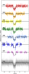 |
Fig. 1 Post-processed light curves of the seven CHEOPS visits and around null phase of the 13 TESS transits in sector 23. From top to bottom: CHEOPS 1 (red), 2 (orange), 3 (yellow), 4 (green), 5 (light blue), 6 (dark blue), 7 (pink), and TESS (grey). Open circles denote binned data (CHEOPS: 10 points, TESS: 30 points), while the solid black lines denote the best model in the joint RV + transit fit (Sect. 4.5). |
3.2.2 CARMENES
CARMENES5 (Calar Alto high-Resolution search for M dwarfs with Exoearths with Near-infrared and optical Echelle Spectrographs) is a double-channel, high-resolution spectrograph at the 3.5 m Calar Alto telescope that covers from 5200 A to 17 100 A in one shot. There is a beam splitter at 9600 Å that divides the stellar light between the optical (VIS, R ≈ 94600) and near-infrared (NIR, R ≈ 80400) channels. Detailed descriptions of the CARMENES instrument at the 3.5 m Calar Alto telescope and the exoplanet survey can be found in Quirrenbach et al. (2010, 2014) and Reiners et al. (2018).
Gl 486 was one of over 300 M-dwarf targets regularly monitored in the CARMENES guaranteed time observation programme. An updated list of past guaranteed time observation and new legacy project targets is included in Marfil et al. (2021). For Gl 486, we initially obtained 80 pairs of VIS and NIR spectra between January 2016 and June 2020 with a time baseline of about 4.5 a. This was the original data set that Trifonov et al. (2021) used in their analysis. We added five additional visits in early May 2021 to these data to anchor CARMENES and new MAROON-X RVs. The typical exposure time in all cases was about 20 min, with the goal of achieving a signal-to-noise ratio of 150 in the J band. A series of short-exposure spectra collected on 02 April 2021 within CARMENES legacy time for another science case were discarded from the analysis because of their low S/N.
All spectra were processed according to the standard CARMENES data flow (Caballero et al. 2016b). We used the latest version of the serval data reduction pipeline (v2.10), re-computed the small nightly zero-point systematics of the CARMENES data, and corrected for them to achieve a metre-per-second precision (e.g. Tal-Or et al. 2018; Trifonov et al. 2018, 2020). Because of the wider wavelength coverage, we were able to measure more indices with CARMENES than with MAROON-X. New indices, apart from dLW, CRX, Hα, Ca II IRT, and Na I D, were the atomic lines of He I D3, He I λ10830 A, and Paβ and the molecular bands of TiO 7050, VO 7436, VO 7942, TiO 8430, and TiO 8860 (Schöfer et al. 2019). We also measured cross-correlation function (CCF) indicators as defined by Lafarga et al. (2020): full width at half maximum (CCF FWHM), contrast (CCF CON), and bisector inverse slope (CCF BIS). Running serval again and, therefore, creating a new template spectrum implies computing new RV velocities and indices. Although very similar to those tabulated by Trifonov et al. (2021), the CARMENES run-1 RVs and indices used here are not identical to what was already published. The MAROON-X and CARMENES RVs are displayed in Fig. 2.
 |
Fig. 2 RV data from CARMENES (green circles), MAROON-X Red (red symbols), and MAROON-X Blue (blue symbols). MAROON-X data are split into runs 1 (circles), 2 (squares), and 3 (triangles). Compare with Fig. S.1 of Trifonov et al. (2021). |
3.3 Interferometry
To extract the planetary mass and radius from the combined RV and transit data, we require the knowledge of the host star’s radius, R*, and mass, M*. These are typically obtained from empirical relations or by using theoretical models to fit other observations of the host star (Mann et al. 2015; Boyajian et al. 2012; Schweitzer et al. 2019). In the case of Gl 486, Trifonov et al. (2021) obtained a precision of ~3% in stellar radius and ~5% in mass, not accounting for systematic errors. Compared to our latest CHEOPS and MAROON-X data, this precision turns out to be the limiting factor in measuring the planetary parameters. As described in Sect. 2, Trifonov et al. (2021) determined R* from L* (Cifuentes et al. 2020) and Teff (Passegger et al. 2019), and M* with the empirical mass-radius relation of Schweitzer et al. (2019). In the present work, however, we directly measured the angular size of Gl 486, from which we determined an R* nearly independent of models or spectral-synthesis-based Teff.
We used the CHARA Array, a long-baseline optical-infrared interferometer located at Mount Wilson Observatory (ten Brummelaar et al. 2005). Observations of Gl 486 were taken on two nights (24 and 27 May 2021) with the MIRC-X beam combiner (Anugu et al. 2020) in the H band using a five-telescope configuration (S1-S2-E1-E2-W1). In interferometry, frequent observations of calibrator stars are needed to measure visibility losses due to non-perfect atmospheric coherence and instrumental effects such as vibration, dispersion, and birefringence. Hence, we used an observing sequence alternating between our target and calibrator stars. We selected calibrator stars from the second version of the Jean-Marie Mariotti Center Stellar Diameter Catalog6 (Bourgés et al. 2014; Duvert 2016; Chelli et al. 2016). The observed calibrator stars were chosen to be bright point sources within 15 deg of the science star on the sky, and they are presented together with their basic properties in Table 4. The data acquisition consisted of taking short, 5 min data sets plus 5 min ‘shutters’ of the science target (Obj) and several calibrator stars (Cal#). In the first run on 24 May 2021, we obtained two sets on the science target in an Obj - Call - Obj - Call sequence, while in the second run on 27 May 2021, we obtained five sets on the science target in a Cal2 - Obj - Obj - Cal3 - Obj - Cal4 - Obj - Call - Obj - Cal3 sequence. Data were reduced and calibrated using version 1.3.5 of the MIRC-X pipeline7 to produce squared visibilities, V2, and closure phases of the science target. During the reduction, we used five coherent coadds, 150 s maximum integration time (each 5 min set was divided into 2 OIFITS8 files), an S/N threshold of 3, and a flux threshold of 5, and we applied the bispectrum bias correction.
Interferometric calibrator stars observed with CHARA.
3.4 Space spectroscopy
To improve the coronal model and better constrain the transition region of Gl 486, we used Hubble low-resolution spectroscopic observations in the ultraviolet. Since there are no public X-ray observations available after the ROSAT observations described by Stelzer et al. (2013), we instead analysed two spectra collected on 15 March 2022 (P.I. Youngblood) with the Hubble Space Telescope Imaging Spectrograph (STIS), the FUV-MAMA detector, and the G140M (1140-1740 Å) and G140L (1150–1730 Å) filters. The spectra were recently made available through the Mikulski Archive for Space Telescopes9 (MAST). On those flux-calibrated spectra, we measured individual atomic lines useful for our purpose as Sanz-Forcada et al. (2003). The line fluxes, Fobs, together with their S/Ns are displayed in Table 5. The remaining tabulated parameters are discussed in Sect. 4.4. The identified species are C II and IV, N V, Al III, and Si II, III, and IV.
Hubble/STIS line fluxes of Gl 486.
3.5 Ground photometry
For the seeing-limited optical photometric monitoring of Gl 486 we collected data with ten different units of Las Cumbres Observatory Global Telescope10 (LCOGT; Brown et al. 2013), the 0.9 m T90 telescope of the Observatorio de Sierra Nevada (OSN; Amado et al. 2021) in Granada, Spain, the 0.8 m Telescopi Joan Oró (TJO; Colomé et al. 2010) at the Observatori Astronomic del Montsec in Lleida, Spain, and the 10 cm Adonis refractor telescope of the Volkssterrenwacht AstroLAB IRIS11 public observatory in Langemark, Belgium. We also added public data of the All-Sky Automated Survey for Supernovae (ASAS-SN; Shappee et al. 2014) and the Wide Angle Search for Planets (SuperWASP; Pollacco et al. 2006). For a summary of the ground photometry data, we invite the reader to consult the bottom part of Table 3.
We did not use other Gl 486 photometry previously compiled by Trifonov et al. (2021). The long-term monitoring data of All-Sky Automated Survey (ASAS; Pojmański 1997) and Northern Sky Variability Survey (NSVS; Woźniak et al. 2004) have poor sampling and large scatter. Because of their short duration, we did not use either observation during and immediately before and after planet transits with the Multicolor Simultaneous Camera for studying Atmospheres of Transiting exoplanets-2 (MuSCAT2; Narita et al. 2019) in May-June 2020, the Perth Exoplanet Survey Telescope (PEST12) in June 2020, LCOGT in May-June 2020, and TJO in April-May 2020.
Mostly because of its relative brightness, there are no useful data of Gl 486 in a number of long-time, baseline, automated, wide surveys such as the Automated Patrol Telescope (APT13; C. G. Tinney, priv. comm.), Hungarian-made Automated Telescope Network (HATNet14; J. Hartman, priv. comm.), MEarth15 (J. Irwin, priv. comm.), Tennessee State University Automated Astronomy Group (TSU16; G. W. Henry, priv. comm.), and Zwicky Transient Facility (Bellm et al. 2019).
The eight light curves used by us are displayed in Fig. 3. The ASAS-SN and SuperWASP North and South data sets were used and described already by Trifonov et al. (2021). These authors also used TJO to cover the ±3σ phase window around the conjunction time predicted by the RV solution at the time of observations, but they performed an intensive monitoring over only four nights. Here, we present a completely new TJO data set that extends for about 11 months, ideal for a long-period determination. We describe below the observations and preliminary data analysis with AstroLAB, LCOGT, and OSN, which were not used by Trifonov et al. (2021), as well as with TJO.
 |
Fig. 3 Used photometric variability sets (Sect. 3.5). From top to bottom: SuperWASP (North and South), ASAS-SN (V and g′), TJO (R), Astro-LAB (V), OSN (V), and LCOGT (B). For homogeneity, we transformed TJO, OSN, and LCOGT (normalised) fluxes to differential magnitudes. |
3.5.1 AstroLab
The Adonis telescope, a commercial 10 cm Explore Scientific ED102 f /7 APO refractor, together with a G2-1600 Moravian CCD camera, provides a field of view of 66 × 44 arcmin2 and pixel size of 1.34 arcsec, which matches the median natural seeing at Langemark, a village of leper (Ypres), at a height above sea level of only 15 m. We used the configuration above and an Astrodon Photometrics V filter to monitor Gl 486 for over six weeks between May and June 2021. Because of the low declination of our target (+09:45) and the high latitude of AstroLAB (+50:51), we always observed it near culmination and at a high air mass (1.6–2.4). The 39 collected images were processed with the LesvePhotometry17 reduction package. For the extraction of the light curve, we used differential photometry relatively to one non-variable comparison star of similar brightness and colour within the field of view.
3.5.2 LCOGT
This network of astronomical observatories has been used to investigate a number of variable astrophysical processes, from supernovae (Valenti et al. 2016), through eclipsing binaries (Steinfadt et al. 2010) and debris discs around white dwarfs (Vanderbosch et al. 2020), to transiting exoplanets (Newton et al. 2019). We refer the reader to Brown et al. (2013) for the technical description of the network telescopes and basic data analysis and the LCOGT website18 for the latest updates. Our B-band photometric observations of Gl 486 with ten 1 m LCOGT robotic telescopes spanned from 22 April 2021 to 27 July 2021 and resulted in 521 images. The data were first divided into ten subsets, one per telescope. Upon visual inspection of each subset, we kept 440 images with an S/N > 8 and not affected by cosmic rays. Aperture photometry on our target and eight reference stars was performed separately for each data set with Astrolmage] (Collins et al. 2017). The median of each data set was then subtracted to create the combined light curve, which has an rms of about 0.010 mag and an approximate Nyquist frequency of 1.5 day−1.
3.5.3 OSN
We also monitored Gl 486 with the T90 telescope at the Observatorio de Sierra Nevada (2896 m). The Ritchey-Chrétien telescope is equipped with a 2k × 2k pixel VersArray CCD camera with a field of view of 13.2 × 13.2 arcmin2 and a pixel size of 0.387 arcsec. The V-band observations were carried out on nine nights in late Spring 2021, with typically 130 exposures per night, and 30 nights during early 2022, with typically 20 exposures per night, each with an integration time of 40 s. We obtained synthetic aperture photometry from the unbinned frames, which were bias subtracted and properly flat-fielded with IRAF beforehand, and selected the best aperture sizes and five reference stars for the differential photometry. In particular, we used the same T90 instrumental configuration and methodology as in previous works involving photometric monitoring of nearby M dwarfs with exoplanets (e.g. Perger et al. 2019; Stock et al. 2020; Amado et al. 2021).
3.5.4 TJO
For the March 2021-April 2022 run of TJO, we collected at least five exposures per observing night with the Large Area Imager for Astronomy (LAIA) and the Johnson R filter. The LAIA is a 4k × 4k CCD camera with a field of view of 30 arcmin and a scale of 0.4 arcsec pixel−1. The images were calibrated with dark, bias, and flat field frames using the observatory pipeline. Differential photometry was extracted with AstrolmageJ using the aperture size and a set of 10 comparison stars selected to minimise the rms of the photometry. We refer the reader to González-Álvarez et al. (2022) for a recent example of TJO being used to study the rotation period of an M dwarf with a transiting planet and RV follow-up.
4 Analysis and results
4.1 Stellar radius
Hanbury Brown et al. (1974) derived the relationship between the distribution of light on the sky, the uniform and limb-darkened disc (UD, LDD), and the squared visibilities, V2, in interferometric observations for measuring apparent angular diameters of stars. The corresponding visibilities for a disc depend on the projected baseline, B′, the linear limb-darkening parameter, µλ, the angular size of the object at a certain wavelength, θλ, and the wavelength of observations, λ, as shown in Eqs. (1)–(4):
 (1)
(1)
 (2)
(2)
 (3)
(3)
 (4)
(4)
where Jα(x) are the Bessel functions of the first kind (α = 1, 3/2). As explained below, the first term in Eq. (1),  , corrects for unknown systematic offsets (di Folco et al. 2007; Woodruff et al. 2008).
In order to determine the stellar angular diameter, we began by creating a large number (N = 3000) of bootstrapped realisations of the calibrated V2 data sets. The uniform disc model was then fitted with the realisations of the data using the Scipy non-linear least-squares minimisation routine (Jones et al. 2001). As part of the fitting process, we also allowed variations in the dependent parameter by sampling the uncertainty in the instrument’s wavelength solution. We fitted each night’s data separately and then when combined. We added the night’s standard deviation to the night results in quadrature with the uncertainty from fitting the entire data set to better capture the true uncertainty in the fit. Since the distribution fits of the determined uniform disc, θUD, and its corresponding floating offset,  , are Gaussian, we tabulate the mean and standard deviations instead of median and 15.8% and 84.1% confidence intervals in Table 6.
We then repeated this process for the limb-darkened disc model using the same technique. We estimated the H-band limb-darkening parameter with the Limb Darkening Toolkit, LDTK (Parviainen & Aigrain 2015), which uses the library of PHOENIX-generated specific intensity spectra by Husser et al. (2013). Hence, the stellar radius determination is not fully model-independent. We provided the LDTK module with first estimates of  , logg, and metallicity, Z. For log g and Z, we used the values in Table 2 and the approximate relation Z = Z⊙ 10[Fe/H], with Z⊙ ≈ 0.013, while for Teff we used the measured θUD in combination with the stellar bolometric luminosity and the Stefan–Boltzmann law
  . We then iterated fitting the limb-darkened diameter until the final
  remained unchanged. This
  , as listed in Table 6, is not identical to the Teff in Table 2, but equal within uncertainties, which supports our determinations. We scaled the errors in µH by five to reflect more realistic values as compared to other limb-darkening grids (e.g. Claret & Bloemen 2011), though this has little impact on the resulting angular diameter, as the uncertainties in the squared visibilities dominate the error in diameter.
The mean and standard deviation for the limb-darkened angular diameter fit, θLDd, with the corresponding µH and  values are again listed in Table 6, while the model for both the limb-darkened and uniform-disc fits and the posterior distributions are shown in Fig. 4. Finally, our measured angular diameter coupled with the corrected Gaia star’s parallax yields a stellar radius of R* = 0.339 ± 0.015 R⊙, which is consistent within less than 1σ with the following value used by Trifonov et al. (2021): R* = 0.328 ± 0.011R⊙.
As noted above, we multiplied the F2/G2 ratio in Eq. (1) by an extra term,  , to account for unknown systematic offsets. Our results indeed showed that
  is at non-unity for both the limb-darkened-disc and uniform-disc fits. In order to determine whether this offset was due to a bad calibrator (e.g. an unknown binary or rotationally oblate object), we did a series of tests on the data sets. First, we calibrated each science target data set independently using the calibrator nearest in time to the science target and found that all calibrators gave mutually consistent results. We then calibrated each calibrator against another to ensure that their response was consistent with point sources, and we found no evidence to reject any calibrator due to that. Lastly, we confirmed that the closure phases of the calibrators were consistent with zero, ensuring us that they are point-symmetric and should not produce spurious results. We suspect that the non-unity
  is a result of the colour mismatch between the calibrators (four early A and one early F dwarfs) and science target (M3.5 V) that is not completely treated in the standard reduction and calibration routines; although, it may also be related to some systematics in the limb-darkening determination of M dwarfs. While the origin of this floating offset is not well understood, we remain confident of the interferometric results, as the stellar diameter is in agreement with past estimates based on independent techniques (e.g. Newton et al. 2015, 2017; Schweitzer et al. 2019; Trifonov et al. 2021, among many others).
Finally, as we put forward in Sect. 2, we determined the stellar mass, M* = 0.333 ± 0.019 M⊕, from R* and the mass-radius linear relation of Schweitzer et al. (2019). The authors derived this relation from 55 detached, double-lined, double eclipsing, main-sequence M-dwarf binaries from the literature. The M*-R* relation of Schweitzer et al. (2019) agrees with (and may surpass) previous relations in the M-dwarf domain by Andersen (1991), Torres et al. (2010), Torres (2013), Eker et al. (2018), and references therein.
 |
Fig. 4 Interferometric determination of the Gl 486 radius with the CHARA Array. Left: MIRC-X squared visibility as a function of spatial frequency (B′/λ, baseline over wavelength). Open grey circles indicate actual measurements, dark blue filled circles with error bars are binned data with standard deviation, and dashed curve and red shadow are our angular diameter fit and its uncertainty. The horizontal dashed lines indicate the visibility at unity (blue) and at unity minus the correction |

CHARA model input and interferometric results.
4.2 Stellar rotation period
The main difficulty in the determination of a robust Prot of Gl 486 lies in its small amplitude of photometric variability. For example, Clements et al. (2017) obtained 69 frames of the star during 5.02 a with the 0.9 m SMARTS telescope at the Cerro Tololo Inter-American Observatory and measured a V-band light curve standard deviation of 11.6 mmag. Díez Alonso et al. (2019) measured greater standard deviations of 32 mmag and 66 mmag with poorer (but public) NSVS and ASAS data, respectively. None of them could conclude anything concerning the star’s photometric variability. Of the photometric data available to Trifonov et al. (2021), they only used the ASAS-SN and SuperWASP (North and South combined) light curves for measuring a stellar rotation period (actually, ‘a proxy obtained from a quasi-periodic representation of the photometric variability’) of Gl 486. However, the signal corresponding to the Prot tabulated by Trifonov et al. (2021), of  days, did not appear in the periodograms of all their data sets, which casted doubts on the Prot determination.
The standard deviations of our eight ground-based light curves (Table 3, Fig. 3) range from 4–10 mmag (LCOGT, OSN, TJO – after subtracting a linear trend from the latter data set) to 28–34 mmag (AstroLAB, ASAS-SN g′) after applying Nσ-clipping filters for outliers (N = 2.5–4.5). We ran generalised Lomb-Scargle (GLS) periodograms (Zechmeister & Kürster 2009) on the joint data sets of SuperWASP and ASAS-SN, with the longest time baseline, and LCOGT, OSN, and TJO, with the smallest scatter. The first joint data set, although it is noisier, allowed us to investigate activity cycles much longer than the stellar Prot, while the second one allowed us to investigate a new range of low-amplitude signals. In the top two panels of Fig. 5, we display the GLS periodograms of the two joint photometric data sets after considering different offsets between the light curves. In the SuperWASP + ASAS-SN periodogram, there is power beyond 300 days, apart from significant signals at ~130 days (as reported by Trifonov et al. 2021) and ~50 days, while the LCOGT + OSN + TJO periodogram shows several significant peaks in the 30–70 days range. A rotation period shorter than 100 days better matches the log R′HK-Prot relations in the literature (e.g. Suárez Mascareño et al. 2016; Astudillo-Defru et al. 2017a; Boudreaux et al. 2022) than the period reported by Trifonov et al. (2021).
In Fig. 5, we also display the GLS periodograms of 13 representative activity indicators associated with Ha, Ca II, Na I, TiO, VO, dLW, and CRX measured on the CARMENES spectra. The TiO indices are the only spectral activity indices that show a forest of (non-significant) peaks around the power maximum of the LCOGT + OSN + TJO periodogram at -50 days. This is in agreement with the weak activity of Gl 486 b and the results of Schöfer et al. (2019), who found that the TiO indices usually are the most sensitive ones to variable activity in weak M dwarfs. However, most of the power of the periodograms falls beyond 100 days. Because of the MAROON-X time sampling, the visits of which were concentrated over a few nights on three short runs much shorter than Prot, a new joint periodogram analysis of the CARMENES and MAROON-X spectral activity indices does not improve the results of Trifonov et al. (2021).
We did a joint fit of our three best light curves, LCOGT (B), OSN (V), and TJO (R), to a double-sinusoidal model with characteristic periods of Prot and Prot/2 (Boisse et al. 2011; González-Álvarez et al. 2022) and a wide uniform Prot prior between 30 days and 60 days. A pair of the most significant peaks in the LCOGT + OSN + TJO periodogram are also 1:2 aliases of each other. Two adjusted sinusoids fixed at the fundamental period and its first harmonic allowed us to remove a large fraction of the photometric jitter amplitude (Boisse et al. 2011 did this for the two first harmonics). The fit was performed using the Juliet19 python package (Espinoza et al. 2019), which uses nested samplers, a numerical method for Bayesian computation that simultaneously provides both posterior samples and Bayesian evidence estimates. Juliet is mostly used for RV and transit best-fit optimisation (Sect. 4.5), but it can also determine rotation periods from light curves. We determined a photometric rotation period of Prot = 49.9 ± 5.5 days and an amplitude of just 3.4 ± 2.4 mmag, which explains the Prot non-detection by Clements et al. (2017, SMARTS) and Díez Alonso et al. (2019, ASAS, NSVS), and the different Prot determination by Trifonov et al. (2021, ASAS-SN, SuperWASP). It is likely that the period measured by them, about three times longer than ours, is associated with a stellar activity cycle. Fig. 6 displays the phase-folded LCOGT, TJO, and OSN data fitted to the two sinusoids.
 |
Fig. 5 GLS periodograms of ground photometry (purple) and CARMENES spectral activity indicator (green) time series. From top to bottom: (a) SuperWASP and ASAS-SN, (b) B LCOGT, V OSN, and R TJO, (c) CARMENES Ca ii IRT[1,2,3], (d) dLW, (e) Hα, (f) CRX, (g) TiO [1,2,3] (TiO 7050, 8430, and 8860), (h) VO [1,2] (VO 7436 and 7942), and (i) Na i D[1,2]. Dark and light green areas at 40–60 days and 100–150 days indicate the Prot and cycle intervals, respectively. Blue dashed horizontal lines mark the 0.1%, 1%, and 10% false alarm probabilities. |
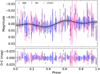 |
Fig. 6 OSN (blue), TJO (violet), and LCOGT (magenta) light curves phase-folded to the double-sinusoidal rotation period (Prot = 49.9 ± 5.5 days). The grey dashed area indicates the fit uncertainty. |
4.3 Stellar abundances
F-, G-, and K-type stars with orbiting Jovian planets are preferentially metal rich (González 1997; Santos et al. 2004; Fischer & Valenti 2005). However, the frequency of low-mass planets, including rocky planets, does not seem to depend on metallicity (e.g. Ghezzi et al. 2010; Mayor et al. 2011; Sousa et al. 2011; Petigura et al. 2018). Likewise, there is no robust indication of a larger frequency of Jovian planets around more metallic M dwarfs (Bonfils et al. 2007; Johnson et al. 2010; Rojas-Ayala et al. 2012; Neves et al. 2013; Courcol et al. 2016); however, see Pinamonti et al. (2019). Jovian planets around M dwarfs are rare (Delfosse et al. 1998; Marcy et al. 1998; Endl et al. 2006; Forveille et al. 2011; Morales et al. 2019; Sabotta et al. 2021), which does not help us in settling the issue. In contrast, small planets around M dwarfs, such as mini-Neptunes and super-Earths, are numerous (Sect. 1). However, the ability to measure a correlation between metallicity and small planet frequency is hampered by the lack of reliable M-dwarf metallicity determinations until very recently. The origin of this absence resides in that M-dwarf atmospheres are more complicated to model than their warmer FGK-type counterparts, though this difficulty is getting easier to overcome with better calibration samples and improved models (Maldonado et al. 2020; Passegger et al. 2022, and references therein).
There are planet-formation models relevant to this work that use different stellar element abundances and ratios as inputs and that predict different planet composition and structure on the assumption that the protoplanetary disc preserves the original stellar abundances (Ida & Lin 2004; Kamp & Dullemond 2004; Chambers 2010; Emsenhuber et al. 2021). Some of these element ratios are Mg/Fe, Si/Fe, C/O, or N/O and will play a role in the future of comparative astrochemistry exoplanetology (Dawson et al. 2015; Gaidos 2015; Thiabaud et al. 2015; Santos et al. 2017; Cridland et al. 2020).
In this work, we applied state-of-the-art M-dwarf element abundance analysis to the high-S/N VIS+NIR CARMENES template spectrum of Gl 486 computed with serval. First, we took the iron abundance with α-enhancement correction, [Fe/H] = −0.15 ± 0.13, from Marfil et al. (2021), which is 1.5σ lower than the mean of seven previously published [Fe/H] values (Table A.4). However, in contrast to the other works (see Passegger et al. 2022), the [Fe/H] values from Marfil et al. (2021) in the range of Teff of our target star are in agreement with the metallicity distribution of FGK-type stars in the solar neighbourhood and correlate well with the kinematic membership of the targets in the Galactic populations. Next, we applied recent techniques for the determination of other element abundances. For internal consistency, apart from the Teff of Marfil et al. (2021), we also used their log g (Table 2) in the following analysis. Our procedure is illustrated in Fig. 7.
First, we used the methodology of Abia et al. (2020) to determine abundances of three neutron-capture elements, namely Rb, Sr, and Zr. In a first step, we determined an average metallicity [M/H] = −0.15 ± 0.10 dex with a number of Fe I, Ti I, Ni I, and Ca I lines, which matches the [Fe/H] of Marfil et al. (2021) and substantiates our choice. Next, we determined the carbon-to-oxygen ratio C/O of Gl 486 with an iterative method that started with a synthetic spectrum with the carbon and oxygen abundances scaled to the metallicity of the model atmosphere. We paid special attention to the strength of CO, OH, CN, and TiO absorption bands. The determined C/O ratio, +0.54 ± 0.05 dex, becomes exactly solar with the latest revision of solar oxygen abundance with respect to the standard value of +0.10 dex (Bergemann et al. 2021). Determining this ratio is vital, as almost all the available carbon in the atmospheres of M dwarfs is locked into CO and, therefore, the abundance of the other O-bearing molecules (TiO, VO, OH, H2O) mainly depends on the C/O ratio. After following all the steps enumerated by Abia et al. (2020), and assuming nonlocal thermodynamic equilibrium (NLTE) for Rb and Sr, we obtained [Rb/M] = +0.15 ± 0.12 dex, [Sr/M] = +0.03 ± 0.14 dex, [Zr/M] = +0.00 ± 0.13 dex, from which we determined the A(X) and [X/H] values in Table 7 with solar values from Lodders et al. (2009). The derived [Rb,Sr,Zr/M] ratios in Gl 486 match the corresponding [Rb,Sr,Zr,M] versus [M/H] relationships of unevolved field stars obtained by Abia et al. (2020, 2021) well.
Next, we used the methodology of Shan et al. (2021) to determine the abundance of V. In M dwarfs, including Gl 486 b, many V I lines exhibit a distinctive broad and flat-bottom shape, which is a result of the hyperfine structure. We used four prominent V I lines at 8093 Å, 8117 Å, 8161 Å, and 8920 Å (1 in air) for the fit, and obtained A(V) = 3.84 ± 0.08. The line-to-line scatter and the errors from the input stellar parameters were added quadratically to determine the abundance uncertainty. With the solar abundances of Asplund et al. (2009), we arrived at [V/H] = −0.08 ± 0.08. The corresponding [V/Fe] = [V/H] − [Fe/H] = +0.07 ± 0.15 is a typical value for stars in the solar neighbourhood (Battistini & Bensby 2015).
Finally, we employed the spectral synthesis method, together with the PHOENIX BT-Settl atmospheric models (Allard et al. 2012) and the radiative transfer code Turbospectrum (Plez 2012) to determine Mg and Si abundances of Gl 486. We measured [Mg/H] = +0.03 ± 0.09 dex and [Si/H] = −0.09 ± 0.13 dex. Further details on the followed steps will be provided by Tabernero et al. (in prep.). To sum up, the composition of Gl 486 seems to be similar to the Sun, but slightly less metallic, although consistent within the error bars.
Element abundances of Gl 486.
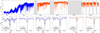 |
Fig. 7 Element abundance determination of Gl 486 b. Top panel: coadded, order-merged, channel-merged CARMENES VIS (blue) and NIR (red) template spectrum. Interruptions (grey areas) are due to strong telluric contamination and inter-order and NIR detector array gaps. Bottom panels: zoomed-in view of six representative, weakly magnetic-sensitive atomic lines from Abia et al. (2020, Rb i, Sr ii), Shan et al. (2021, V i), Passegger et al. (2019, Mg i), and Marfil et al. (2021, Fe i, Ti i). Black dashed lines are the synthetic fits. |
4.4 Stellar coronal emission
To quantify the coronal activity of Gl 486, we searched through public archives of space-borne high-energy observatories (Extreme Ultraviolet Explorer, Chandra, XMM-Newton, Neil Gehrels Swift, eROSITA/Spektr-RG) and found a ROSAT X-ray (5-100 A) upper limit by Stelzer et al. (2013); see also a non-detection reported by Wood et al. (1994). We converted it into an upper limit of the X-ray luminosity with the corrected Gaia distance. The expected X-ray luminosity considering the stellar rotation period of ~50 days, together with the V − Ks colour and L* of Gl 486 and the LX-Prot relation of Wright et al. (2011), is logLX = 27.44 erg s−1. The value is higher than the upper limit calculated by Stelzer et al. (2013), but still consistent given the spread of X-ray luminosity observed in the rotation-activity diagram, of up to one order of magnitude (Table 2).
We also derivedourownupperlimitforthe extreme ultraviolet (EUV, 100–920 Å) luminosity from a coronal model informed by the Hubble/STIS data presented in Sect. 3.4. On the G140L and G140M spectra, we measured the emission measure, EM, defined as:
 (5)
(5)
where Ne and NH are the electron and hydrogen densities (in cm−3), respectively, and V is the volume. Although most measured C, N, Al, and Si lines do not reach the usually required 3σ detection (Table 5), the combined fluxes give a consistent emission measure distribution in the log T (K) = 4.1–5.5 range following the techniques described by Sanz-Forcada et al. (2003); the resulting emission measure distribution is illustrated by Fig. 8 and tabulated with their uncertainties in Table A.5. To evaluate the coronal part of the model, we tried different values of T and EM consistent with the upper limit of LX ≈ 4.17 × 1026 erg s−1 reported by Stelzer et al. (2013). Since the low level of stellar activity indicates a low coronal temperature, we fixed it at a typical quiet solar value of log T (K) = 6.2, which implies log EM(cm−3) = 49.0 with a solar photospheric abundance. Calculated coronal abundances are [C/H] = +0.0 ± 0.3, [N/H] = +0.0 ± 0.3, [Si/H] = +0.2 ± 0.4, and [Al/H] = +0.6 ± 0.9. A more realistic value of coronal abundances would probably imply an Fe enhancement, similar to the solar corona, which would in turn imply an EM value about one order of magnitude lower, but with little impact on the overall X-ray luminosity. With this coronal model, we predicted a more realistic upper limit of the EUV luminosity of 1.45 × 1027 erg s−1. The results are similar to those achieved when applying the LX–LEUV relation of Sanz-Forcada et al. (2011). In the 100–504Å spectral range, which is involved in the formation of the He λ10830 Å triplet in planet atmospheres (Nortmann et al. 2018), the upper limit of the luminosity amounts to 1.27 × 1027 erg s−1.
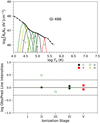 |
Fig. 8 Stellar coronal emission of Gl 486 from ultraviolet spectroscopy. Top: emission measure distribution from Hubble/STIS data. Thin, coloured lines represent the relative contribution function for each ion (the emissivity function multiplied by the emission measure distribution at each point). Numbers within the graph indicate the ionisation stages of the species. Bottom: observed-to-predicted line flux ratios for the ion stages in the upper figure. The dashed lines denote a factor of two. |
4.5 Planet radius and mass
We combined the CARMENES and MAROON-X RV data with the CHEOPS and TESS photometric transit data. As in Trifonov et al. (2021), we did not use HARPS or HIRES RV data, nor any of the plethora of noisier photometric data sets collected for the transit analysis (LCOGT, MuSCAT2, etc.) or by us for the stellar Prot determination. As already noticed by Trifonov et al. (2021), the GLS periodograms of the CARMENES and MAROON-X data are dominated by the planet signal at ~ 1.47 days and its 1 day alias at ~3.14 days (see their Fig. S4). Once the planet signal is subtracted, two signals with a low significance of 1-10% remain. One of them is the yearly alias at ~360 days, which is visible in the RV window, while the other signal at ~ 100 days may correspond to a stellar activity cycle or twice Prot (Sect. 4.2 and below).
We implemented four different models, which are sorted by increasing complexity in Table 8, from one planet in circular orbit to one planet in eccentric orbit and a GP associated with the stellar photometric variability and applied to the RVs. As for the stellar Prot analysis (Sect. 4.2), the fits of the four models were performed using Juliet. For the dynamic nested sampling, we used dyne sty, which is a generalisation of the nested sampling algorithm in which the number of ‘live points’ varies to allocate samples more efficiently (Higson et al. 2019). To double check the results obtained with Juliet, we also used the Exo-Striker20 exoplanet toolbox (Trifonov 2019; Trifonov et al. 2021), a free Python tool with a fast graphical user interface for maximum productivity.
We modelled the planetary transits from the flattened photometric data to measure the orbital period (P) and relative planet-to-star size (p = Rb/R*), the time of transit centre of the planet (t0,b), the inclination of the planetary orbital plane (ib), and the star-planet separation-to-radius ratio (ab/R*). The Juliet and Exo-Striker tools use the batman package (Kreidberg 2015) to this end. The stellar limb-darkening coefficients (quadratic law), q1 and q2, were parameterised following Kipping (2013). We tested using the output of the Limb Darkening Calculator21 as q1 and q2 priors with the star’s Teff, log g, and [Fe/H] from Table 2, Kurucz ATLAS9 models, and quadratic limb-darkening profiles. For the test, we also used the SDSS i′ band-pass response function as a proxy for those of TESS (T) and CHEOPS. However, probably due to width of the space mission response functions encompassing ranges of 4000–5000 Å22, the stellar density posterior, p*, did not match its prior from R* and M* in Table 2 (see below). Therefore, we eventually used uniform priors between 0 and 1 for the quadratic limb-darkening parameters. As a sanity check, we compared our q1 and q2 parameters with those calculated with limb-darkening23, a Python code developed by Espinoza & Jordán (2015). We used the stellar parameters in Table 2, the TESS and CHEOPS response functions from the Filter Profile Service of the Spanish Virtual Observatory24 (Rodrigo et al. 2012; Rodrigo & Solano 2020), and the A100 fitting technique (i.e. limb-darkening coefficients from ATLAS models and interpolating 100 µ-points with a cubic spline as in Claret & Bloemen 2011). The quadratic parameters computed with limb-darkening (q1,tess = 0.37, q1,cheops = 0.46, q2,tess =0.16,q2,cheops =0.21) are identical within uncertainties to the ones determined by us with uniform priors between 0 and 1, which, a posteriori, justifies our approach.
In the fits with Juliet, instead of determining the planet’s relative radius and impact parameter (b ≡ (ab/R*)cosib), we used the parameterisation of Espinoza (2018) and Espinoza et al. (2019), and determined r1 and r2, which vary between 0 and 1 and are defined to explore the physically meaningful ranges for Rb/R* and b. As Trifonov et al. (2021), we adopted dilution factors, Dtess and Dcheops, of 1.0, which translates into no contamination in the (relatively large) TESS and CHEOPS photometric apertures that may mimic a possible planetary transit (see Sect. 4.6 for a companion search). We added a photometric jitter to the nominal flux error bars, σTESS and σcheops, for symmetry with the RV jitter parameters, σcarmenes and σmaroon-x, although the inclusion of the eight additional parameters (one from TESS, seven from CHEOPS) barely modifies the results of the fits. We defined a prior on the stellar density, ρ*, instead of the scaled semi-major axis of the planets, ab/R*. For the periodicity associated with the lpl+GP and lpl+e+GP models, we used a Gaussian Prot,gp prior centred on 49.9 days and a width of 10.0 days from the photometric analysis in Sect. 4.2. We used a quasi-periodic kernel introduced by Foreman-Mackey et al. (2017) of the following form:
![$k{ & _{i,j}}\left( \tau \right) = {{{B_{{\rm{GP}}}}} \over {2 + {C_{{\rm{GP}}}}}}{e^{ - \tau /{L_{{\rm{GP}}}}}}\left[ {1 + {C_{GP}} + \cos {{2\pi \tau } \over {{P_{{\rm{rot}}}}}}} \right],$](/articles/aa/full_html/2022/09/aa43548-22/aa43548-22-eq67.png) (6)
(6)
where τ = |ti − tj| is the time lag, BGP and Cgp define the amplitude of the GP, LGP is a timescale of the amplitude modulation of the GP, and Prot is the period of the quasi-periodic modulations. In order to simplify the GP equation, we fixed the parameter Cgp to 0, and, therefore:
![$k{ & _{i,j}}\left( \tau \right) = {{{B_{{\rm{GP}}}}} \over {2 + {C_{{\rm{GP}}}}}}{{\rm{e}}^{ - \tau /{L_{{\rm{GP}}}}}}\left[ {1 + \cos {{2\pi \tau } \over {{P_{{\rm{rot,GP}}}}}}} \right].$](/articles/aa/full_html/2022/09/aa43548-22/aa43548-22-eq68.png) (7)
(7)
Finally, for the non-circular models, we set uniform priors on eccentricity, e, from 0.00 to 0.15 (three times the upper limit of Trifonov et al. 2021) and on the argument of periapsis, ω (periastron angle), from 0 to 2π.
Table 8 summarises the four different models with the corresponding values of Bayesian log-evidence, In Z (Jeffries 1961; Trotta 2008), and the number of parameters, Npar. As in Buchner et al. (2014), we adopted the scale of Jeffries (1961): a Bayesian log-evidence difference, ΔlnZ, above 2.0 is ‘decisive’; above 1.5, it is ‘very strong evidence; between 1.0 and 1.5, it is ‘strong evidence’; and between 0.5 and 1.0, it is ‘substantial evidence’. In the case of ΔlnZ < 1.0, one must keep the simplest model with the smallest Npar. In previous works on CARMENES RV follow-up of transiting planets detected by TESS, even more conservative criteria of ΔlnZ > 2.5 or 5.0 for decisive difference between models has been used (Kossakowski et al. 2021; González-Álvarez et al. 2022; Kemmer et al. 2022). Such conservative criteria in Bayesian analyses applied to exoplanets can be traced back to previous works (e.g. Gregory 2005; Feroz et al. 2011).
The ln Z of the four models vary within a small range, but the models with the highest ln Z are 1pl + GP and 1pl + e + GP, which are decidedly better than lpl and lpl + e (|∆lnZ| ~ 15). Since the Bayesian log evidences of the two best models vary by just |∆ln Z| ~ 0.5, we selected 1pl + GP, with a lower number of parameters than 1pl + e + GP, as our working model.
The rms of the lpl+GP observed-minus-calculated (O-C) residuals are 693 ppm and 411 ppm for TESS and CHEOPS, and 1.22 m s−1 and 0.74m s−1 for CARMENES and MAROON-X, respectively. The phase-folded TESS + CHEOPS and CARMENES + MAROON-X data with the corresponding best model fit are shown in Fig. 9, while the corner plot depicting the most relevant posterior distributions and derived parameters is shown in Fig. A.3. In total, the lpl+GP model has one stellar, 22 photometry-instrumental, 14 RV-instrumental, four GP, and seven planet parameters, five of which were fixed (e, ω, Dtess, Dcheops, and Cgp), which makes 43 free parameters. The priors, posteriors, units, and description of each parameter are given in Table A.6 (see Espinoza et al. (2022) for a recent application of Juliet and an explanation of the CHEOPS and TESS µ and σ units − mflux and σw in their nomenclature). According to Espinoza (2018), the extra jitter (σw) is the term added in quadrature to each of the error bars of data points for speeding up the computation of the model log evidence (and, therefore, the covariance matrix is diagonal and the noise is white). The extra RV jitter terms added when no GP is included become significantly higher than the values in Table A.6. For example, σcarmenes reaches as high as 1.41 ± 0.19 m s−1 in the lpl (no GP) model, which is in line with the typical scatter of CARMENES VIS RV measurements (Reiners et al. 2018) and the actual rms measurement at 1.22 m s−1.
The most relevant fitted parameters for the lpl+GP model are tabulated again, together with derived and additional planet parameters, in Table 9. The planet radius and mass are  and
and  respectively, from which we derive values of bulk density, surface gravity, and escape velocity that are only slightly larger than those of Earth (ρb ~ 1.2ρ⊕, gb ~ 1.7 g⊕, ve,b ~ 1.5 ve,⊕). However, the instellation is over 40 times higher, which translates into a Bond albedo-corrected Teq higher than on Earth (Sect. 5.3). Apart from the parameters enumerated above, we also tabulate the transit probability, Ptransit, transit depth, ∆transit, transit duration from the first to the last contact, T14, and the ingress and egress duration, T12 = T34, computed as Winn (2010).
In Table A.6, the value of Prot,GP from the applied GP to the RVs, of  days, is consistent within 1σ with Prot,phot from LCOGT+OSN+TJO optical photometry, which is of 49.9 ± 5.5 days, as expected from the normal prior for Prot,GP based on Prot,shot. The Gp parameter that accounts for the timescale of the cyclic variations,
  days, is in agreement with the period of 131 days reported by Trifonov et al. (2021) and the RV signal at ~100 days. This long periodicity may actually be real and correspond to an activity cycle or the timescale of photospheric spots. On the other hand, the GP parameter that accounts for the activity semi-amplitude,
  m s−1, is also in agreement with the expected RV semi-amplitude from the log R′HK relation of Suárez Mascareño et al. (2018), in the 1.0–2.5 ms−1 range, and with the low amplitude of photometric variability (Saar et al. 1998; Jeffers et al. 2022). As a sanity check, we also modelled our data under the 1pl + GP scenario using different Prot,GP priors: normal around 130 days and uniform from 50 days to 130 days. In all cases, the fitted and derived parameters were identical within 1σ uncertainties and, therefore, independent of the stellar cyclic variation.
Finally, we compared the 43 parameters that the two models have in common and are decisively the best, namely 1pl+GP (our working model) and 1pl+e+GP. In all cases, the differences between the parameters of the two models are well within 1σ. These differences also apply to the derived parameters in Table 9. In particular, the differences in Rp and Mp of the two models are in the fourth significant figure, about three orders of magnitude smaller than the uncertainties. The only two parameters that significantly differ between the two models are, obviously, e and ω. For the 1pl+e+GP model, we measured  deg and
  (they were fixed to 90 deg and 0, respectively, in the 1pl+GP model). From this eccentricity value, we can infer a 1σ upper uncertainty e < 0.022 for Gl 486 b. This upper limit is more constraining by a factor of two than the value determined by Trifonov et al. (2021), who imposed e < 0.05.
There might also be a concern about the pre-detrending of the CHEOPS transit photometry prior to the joint transit+RV fit. In our case, we first detrended the CHEOPS light curves using the add_glint function of PyCheops (basically a cubic spline against the spacecraft roll angle – Sect. 3.1.1) and then used these detrended light curves in our joint fit with juliet. Although such a pre-detrending approach is common in the literature, it may result in underestimating our uncertainties on the transit parameters (and derived planet parameters, including the radius) by not accounting for the covariances between the detrending and transit parameters. Therefore, we modelled the correlated noise in the CHEOPS light curves simultaneously with the joint transit + RV fit and compared with the results in Table 9. For that, we re-ran a modified 1pl+GP model by using a second GP, as in Leleu et al. (2021). They used a Matérn-3/2 kernel against roll angle plus a polynomial in time and x–y photocentroid position, while we only used an exponential-squared kernel in linear time and the seven CHEOPS light curves. For each light curve, we added two additional parameters (i.e. 14 in total) with very wide log-uniform priors between 10−6 and 106 (σCHEOPSi,GP) and between 10−3 and 103 (ρCHEOPSi,GP). We compared the posteriors of the rest of parameters with the results of the 1pl+GP fit in Table A.6 and, again, found no appreciable differences within 1σ. This result is in line with the findings of Lendl et al. (2020), who also compared the results of applying different GP kernels and decorrelation techniques, as well as pre-detrending with PyCheops, and obtained values that are fully compatible. All in all, Gl 486 b is a well-characterised warm planet at the boundary between exoearths and super-Earths.
Log-evidence and number of parameters of RV+transit Juliet models.
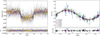 |
Fig. 9 Phase-folded transit and RV data and lpl+GP model fits. Left: light-curve model fit (black line) and CHEOPS+TESS data with the same symbol colours as in Fig. 1 (grey: TESS; rainbow colours: CHEOPS). Right: RV-curve model fit (black line with ±1σ uncertainty marked with a grey shaded area) and CARMENES+MAROON-X data with the same colours as in Fig. 2. Error bars include original RV uncertainties (opaque) and jitter added in quadrature (semi-transparent). |
Fitted and derived planet parameters of Gl 486 b.
4.6 Search for additional companions
Due to its proximity, the star Gl 486 has been the subject of several searches for close companions, sensitive to very-low-mass stars, brown dwarfs, or planets. The results of the Doppler surveys by Marcy & Benitz (1989) and Davison et al. (2015) were not useful for this purpose because they only collected one RV point each. Bonfils et al. (2013), although they collected four RV points with HARPS, set a preliminary upper limit to the short-term RV scatter of a few m s−1. Jódar et al. (2013) and Rodríguez et al. (2015) also looked for companions (and debris discs) around Gl 486 with the FastCam lucky imager in the red optical and with the ESA Herschel space mission in the mid-infrared, both with null results. However, the imaging observations by Dieterich et al. (2012) and Ward-Duong et al. (2015) were more restrictive for the presence of close companions, as illustrated by the left panel of Fig. 10. Dieterich et al. (2012) used NICMOS on the Hubble with the F180M near-infrared filter, and Ward-Duong et al. (2015) used archival adaptive optics imaging obtained with the KIR infrared imager of AOB/PUEO at the Canada-France-Hawai’i Telescope and the [Fe II] narrow filter at 1.6 µm. Both of them established magnitude differences and angular separation limits for which hypothetical companions could be ruled out for Gl 486, which ranged from 0.96 mag at 0.15arcsec (1.2au) to 10.8mag at 3.0-4.0 arcsec (24-32 au). Moreover, Ward-Duong et al. (2015) complemented their AOB/PUEO survey with a common proper motion search on SuperCOSMOS digitised photographic plates (Hambly et al. 2001) to extend their limits at 7.5-7.8 mag from 4.0 arcsec to 19.9 arcsec (161 au). According to D. Ciardi (priv. comm.), beyond a few arcseconds, it would be very hard to beat Hubble without spending a very long time on Keck, Palomar, Lick, or Paranal observatories with adaptive optics facilities.
We also performed our own multiplicity analysis with Gaia EDR3 data. First, we searched for any previously undetected close multiplicity. We analysed the distribution of four representative Gaia EDR3 astrometric quality indicators of over 2200 Carmencita stars: The goodness-of-fit statistic of the model with respect to along-scan observations (astrometric_gof_al), the along-scan chi-square value (astrometric_chi2_al), excess noise of the source (astrometric_excess_noise), and the significance of excess noise (astrometric_excess_noise_sig). Because of the similarity of the four Gaia EDR3 astrometric quality indicators, in the right panel of Fig. 10 we only plot the distribution of astrometric_gof_al.
Carmencita is the CARMENES input catalogue of M dwarfs observable from Calar Alto, from which we selected the CARMENES survey targets, including Gl 486 and the brightest stars in their spectral type bin and those without physical or visual companions at less than 5 arcsec (Caballero et al. 2016b; Alonso-Floriano et al. 2015; Reiners et al. 2018). Close binaries with angular separations of ρ ~ 0.05–0.50 arcsec that are unresolved by Gaia but known to have companions (e.g. resolved instead with adaptive optics, lucky imaging, speckle, or with Hubble, or unresolved with imaging but known to be long-term spectroscopic binaries) in general have relatively large astrometric quality indicator values. The low values of Gl 486 are typical of stars with no companions at close separations. This is in line with its re-normalised a posteriori mean error of unit weight error (RUWE) of 1.094 and below the conservative value for stars with well-behaved astrometric solutions at ~1.4 (Arenou et al. 2018; Lindegren et al. 2018; Cifuentes et al. 2020; Penoyre et al. 2022) and the previous non-detections by Dieterich et al. (2012), Jódar et al. (2013), Rodríguez et al. (2015), and Ward-Duong et al. (2015).
Next, we searched for Gaia common parallax and proper motion companions to Gl 486 at wide separations not explored before, as in Montes et al. (2018) and Cifuentes et al. (2021). In particular, we searched between 5 arcsec (there are no closer Gaia EDR3 sources) and the angular separation that corresponds to a projected physical separation of 100 000 au (Caballero 2009) with the following criteria: A proper motion ratio of Δµ/µ < 0.15, a proper motion position angle difference of APA < 15 deg (see Eqs. (1) and (2) in Montes et al. 2018), and a distance ratio of Δd ≡ |dA − dB| < 0.10 (i.e. within 0.8pc for this target). This search was complete down to the Gaia EDR3 G-band completeness limit at 20.41 mag (Gaia Collaboration 2021b), which translates into an absolute magnitude of MG ≈ 20.87 mag at the distance of Gl 486 (Pecaut & Mamajek 2013; Cifuentes et al. 2020). This absolute magnitude corresponds to sub-stellar objects at the L-T spectral type boundary. Eventually, we ruled out the presence of stellar and high-mass brown-dwarf companions to Gl 486 from the limit of the Hubble observations at 24–32 au up to 100 000au. At 8pc, this projected physical separation implies a search radius of 3.5 deg and, with a total proper motion of 1100 mas a−1, projection effects of about 8 mas a−1, which is much lower than Δµ ~ 160 mas a−1 from the Δµ/µ criterion. Therefore, we are not missing any possible wide companion.
We searched for additional planets in the system at much shorter separations with our RV data. The GLS periodogram of the RV residuals of the lpl+GP fit, displayed in the left panel of Fig. 11, does not show any significant signal in the investigated frequency domain (which corresponds to periods in the 1.1-1000 days range). To estimate the sensitivity of our RV data to additional planets in the system, we computed detection limits following the injection and retrieval procedure presented by Bonfils et al. (2013) and used by Kossakowski et al. (2021). In short, we injected signals to the actual CARMENES + MAROON-X RV data set corresponding to circular orbits (e = 0) with increasing semi-amplitude K until they were detected with a 99.9% confidence level. We performed the experiment both using the measured RVs and the residuals after subtracting a new lpl model of Gl 486 b with the lpl+GP posteriors as narrow priors. We did not use the lpl+GP model in the experiment because the GP may erase any additional long-term signal besides the stellar rotation period. The test on residuals indicates that additional planets in the system above the mass range of ~2-5 M⊕ can be excluded for periods within the time span of the data at ~2000days, and above ~10M⊕ for periods up to 10 000 days, although in this last case, eccentric orbits may impact the results. These periods correspond, through Kepler’s third law of planetary motion, to semi-major axes of ~2.2 au and 5.5 au, respectively, which are 130–320 times greater than the orbital semi-major axis of Gl 486 b.
Finally, we extended the time baseline of the RV monitoring for a better investigation of periods longer than ~2000 days. For that, we added the HIRES and HARPS RVs compiled by Trifonov et al. (2021) to our CARMENES and MAROON-X data sets, which led us to extend the time span from 1967 days (243 RVs) to 8529 days (281 RVs). Because of the greater noise of the HIRES and HARPS data with respect to CARMENES and MAROON-X, the improvement in the injection is appreciable only beyond 5000 days. With the additional data, we excluded planets with minimum masses of ~30M⊕ with periods up to 20 000 days (~11 au). We also considered adding 12 additional RVs from the SOPHIE and ELODIE Archive25 to the new injection, but they are even noisier than those of HARPS and HIRES and overlap in time. The injection analysis is illustrated in the right panel of Fig. 11.
As discussed below, Gl 486 will be observed again by TESS in Sector 50. These new observations, together with the CHEOPS and TESS data used in this paper, photometric data from MuSCAT2/Telescopio Carlos Sánchez and LCOGT presented by Trifonov et al. (2021), and three new CHEOPS visits scheduled for 2022 will allow us to search for new low-mass planets in the system, especially through transit time variations. This analysis will be part of a forthcoming publication.
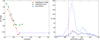 |
Fig. 10 Imaging and astrometric searches for close brown dwarf and stellar companions. Left: contrast curves of Gl 486 from Dieterich et al. (2012, NICMOS/HST F180M, red circles), Ward-Duong et al. (2015, PUEO/CFHT [Fe II], green squares), and our common-parallax and proper-motion search at wide angular separations with Gaia EDR3 data (blue triangles). Right: distribution of Gaia EDR3 goodness-of-flt statistic of model with respect to along-scan observations (astrometric_gof_al) of over 2200 Carmencita M dwarfs. Light blue: all Carmencita stars; dark blue: Carmencita stars with companions at less than 5 arcsec (Caballero et al. 2016b; Cortés-Contreras 2016; Jeffers et al. 2018; Baroch et al. 2018, Baroch et al. 2021). The vertical dashed line marks the value for Gl 486. |
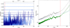 |
Fig. 11 Signal injection on RV data and planet retrieval. In both panels, the CARMENES+MAROON-X and CARMENES+MAROON-X+HARPS+HIRES data sets are plotted with dark and light colours, respectively. Left: GLS periodogram of the RV residuals of the lpl model (blue). Horizontal lines of different thicknesses mark the 0.1%, 1%, and 10% false alarm probabilities, from top to bottom, while the red vertical line marks the orbital period of Gl 486 b. Compare with panels A-H of Fig. S4 of Trifonov et al. (2021). Right: Detection limits on minimum mass following Bonfils et al. (2013) for the RV data of Gl 486 before (grey) and after (green) subtracting the lpl model. Any planet above the green lines is excluded with 99.9% confidence. The blue dashed line is the minimum mass corresponding to a semi-amplitude of 1.22 m s−1 |

5 Discussion
5.1 Comparison with other exoplanets
For a proper comparison of Gl 486 b with exoplanets from the literature, we compiled all the confirmed exoplanets with measured mass and radius. For that, we started off with the complete list of exoplanets provided by the Exoplanet Archive26. Firstly, we discarded unconfirmed Kepler and TESS candidates by choosing soltype == Published Confirmed. Secondly, we selected only the exoplanets discovered by transits, RV, or transit timing variations using the discoverymethod column. Next, we only kept those for which values of both mass (pl_masse) and radius (pl_rade) were tabulated. Among them, we chose those whose masses were derived directly from observations and not inferred from their radii by selecting planets with tabulated densities pl_denslim == 0. Finally, we selected the default set of planetary parameters tabulated in the Exoplanet Archive by selecting default_flag == 1. We only chose the parameters from a source different to the default choice for Kepler-7 b, Kepler 51 b, c, and d, Kepler 138 b, and LTT 3780 b and c.
We added the uncertainties in stellar mass by hand for the hosts of 23 planets, including the seven planets in the TRAPPIST-1 system, since they were incorrectly rounded when downloaded. Additionally, we incorporated four planets not yet included in the Exoplanet Archive: GJ 3929 b (Kemmer et al. 2022), TOI-1759 b (Espinoza et al. 2022), and TOI-1238 b and TOI-1238 c (González-Álvarez et al. 2022). In total, the sample contains 651 confirmed transiting exoplanets with mass and radius determination, displayed in Fig. 12. Coloured symbols stand for planets with mass and radius uncertainties of less than 30%.
As already mentioned by Trifonov et al. (2021), Gl 486 b falls in the expected region for rocky planets with an Earthlike composition, which is well traced towards Martian masses by Gl 637 b and the seven planets in the TRAPPIST-1 system. Gl 486 b seems to be placed in the most massive extreme of the sequence of pure rocky planets. Planets with greater masses are more scattered in the mass-radius diagram as they are probably made of varied mixtures of shallow-to-deep gas and ice envelopes, rocky mantles of various depths, and metallic cores of different sizes.
While our relative radius error of Gl 486 b matches the bulk of those for other well-characterised small transiting planets with Rp ≲ 2R⊕, it is one of the very few transiting planets among all the sizes with an interferometric determination of its stellar host radius, namely 55 Cnc, HD 189733, HD 209458, HD 219134, HD 97658, and Gl 436 (von Braun et al. 2011, 2012; Boyajian et al. 2012, 2015; Ligi et al. 2016; Ellis et al. 2021). Due to the precision of the CARMENES and MAROON-X RV data, together with the relative brightness and very weak activity of Gl 486, our relative mass error is comparable to the most precise determinations available to date among low- and intermediate-mass planets with Mp ≲ 100M⊕, at about 4%. The sources and propagation of error of radius and mass for Gl 486 b in particular and for transiting planets in general are detailed in Appendix B.
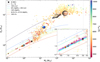 |
Fig. 12 Mass-radius diagram of all currently known transiting exoplanets with mass determination (from RV or transit time variations), in comparison with the Solar System planets. Filled circles with error bars colour-coded by their host’s Teff are planets with mass and radius uncertainties of less than 30%, and open grey circles are the others. The filled black star is Gl 486 b. Dashed coloured curves are theoretical models of Zeng et al. (2019), as specified in the legend. The Earth-like model is orange. The grey vertical dashed line is the deuterium burning mass limit at 13 MJup (‘planet’-brown-dwarf boundary; see Caballero 2018 and references therein). In the inset, we zoom in around the smallest planets and add mass-radius relationships informed by stellar abundances (Sect. 5.2). We plot median and 1σ error regions following nominal relative abundances of Fe, Mg, and Si of the host star without (pink) and with (cyan) the empirical correction of Adibekyan et al. (2021) based on well-characterised super-Earths. The two outliers with very high densities and M ~ 2.0 M⊕ are Kepler-1972b and c, which are two transiting planets with masses determined from transit time variations (Leleu et al. 2022). |
5.2 Planet interior modelling
We modelled the interior of Gl 486 b with available data. First, we compared the planet mass and radius from Sect. 4.5 to the stellar abundances from Sect. 4.3. If the planet reflected the relative abundances of refractory elements of its host star (i.e. Fe, Mg, Si), mass-radius curves informed by stellar abundances would fit the planet data (Dorn et al. 2015). As shown in the inset of Fig. 12, this is the case of Gl 486b when the uncertainties of the planet parameters match the mass-radius relation informed by stellar proxies (pink). Recently, empirical studies have demonstrated that planets are likely enriched in iron compared to their stellar abundance proxies (Plotnykov & Valencia 2020; Adibekyan et al. 2021). If we use the empirical correction suggested by Adibekyan et al. (2021), the planetary data fit the iron-enriched mass-radius relation (cyan) better.
Second, we computed an inference analysis of interior parameters. Our 1D planetary interior model was based on the generalised Bayesian inference method of Dorn et al. (2015, 2017), with updates from Dorn & Lichtenberg (2021). We described the planet in hydrostatic equilibrium with three possible components: an upper layer, a mantle of variable composition, and an iron-dominated core.
In our model, the upper layer is made of pure H O, for which we used the equation of state of Haldemann et al. (2020). For Gl 486 b, the Teq of about 700 K (see Table 9 and Sect. 5.3) forces any water to be present as a steam atmosphere. We assumed that the transit radius derived in Sect. 4.5 is at a pressure of ptransit = 1 hPa (i.e. 10−3 bar). By assuming anything volatile in the upper layer to be in the form of water, we provide upper limits on the possible amount of water.
Also in our model, the mantle is made of MgO, SiO, and FeO that form different minerals. To compute stable mineralogy for a given composition, pressure, and temperature of the solid mantle, we used the Perple_X thermodynamical model of Connolly (2009), which employs equations of state from Stixrude & Lithgow-Bertelloni (2011). For the different components of the liquid mantle, we used a compilation of equations of state from Melosh (2007), Faik et al. (2018), Ichikawa & Tsuchiya (2020), and Stewart et al. (2020) and the additive volume law to compute mixtures from Dorn & Lichtenberg (2021). Finally, for the core we also used a compilation of different equations of state to account for different phases of iron (Dorogokupets et al. 2017; Hakim et al. 2018; Ichikawa & Tsuchiya 2020; Kuwayama et al. 2020; Miozzi et al. 2020). We allowed the mantle to vary in iron content, which is why an iron-rich mantle with no core was allowed in the posterior solution. Whenever we allowed for water to be present in dissolved form in possible magma layers, we followed the approach of Dorn & Lichtenberg (2021), while the partitioning of water between the surface reservoir and the magma was determined by solubility laws (Kessel et al. 2005; Lichtenberg et al. 2021; Bower et al. 2022). We accounted for the fact that water increases the melt fraction by lowering the melting temperature (Katz et al. 2003). Also, the presence of water decreases melt density, which is nearly independent of pressure and temperature (Bajgain et al. 2015).
We tested three different planet interior scenarios in increasing order of complexity. Scenario MR-S was the baseline model of a rocky interior with a thin volatile layer and no further restrictions. In scenario MRA-S, we added the constraints from nominal relative stellar abundances (Fe, Mg, Si), which significantly reduced uncertainty on interior parameters and also caused the mantle mass to significantly increase at the expense of the core mass. The upper layer also became less massive. However, this scenario did not take into account the abundance enrichment suggested by Adibekyan et al. (2021), which is necessary to locate Gl 486 b within a modelable Mp-Rp trend. As a comparison, Demangeon et al. (2021) did not measure the LP 98-59 Mg and Si abundances directly, but instead adopted the mean abundances of Mg and Si of a large list of thin-disc stellar analogues as a proxy. Finally, in scenario MRA-SH, apart from adding the stellar abundance constraints, we allowed water to be not only present on the surface but also to be dissolved in molten parts of the mantle magma ocean, provided the temperature and pressure conditions did not prevent us from doing so. This added complexity corrects possible water mass fractions by roughly an order of magnitude. Therefore, this addition, which was recently proposed by Dorn & Lichtenberg (2021), is critical for warm and hot planets such as Gl 486 b: by neglecting deep water reservoirs in the mantle, bulk water estimates lead to underestimated values. Unfortunately, the actual amount of water critically depends on the stellar proxy of refractory elements (and whether they are added as constraints), how water is modelled in the interior, and the atmosphere mass loss during the entire life of the system (as oxygen and hydrogen loss in the Venus atmosphere) and, therefore, on the incoming stellar flux, as well as the atmospheric XUV (5–920 Å) heating and eroding efficiency (Kasting & Pollack 1983; Barabash et al. 2007; Sanz-Forcada et al. 2011). While the mantle and core equations of state are based on the knowledge of planets of our Solar System, we must still learn more about M-dwarf stellar abundances and their impact on planet interior models, as well as about XUV radiation and its effect on planet atmospheres.
Under the MRA-SH model, with the Gl 486 b mass and radius, Fe, Mg, and Si relative stellar abundance constraints, and water allowed to dissolve in molten rock, we computed confidence regions for mass fractions of the water upper layer, log  , mantle
  , and core,
  . The core radius relative to the planet radius is
  . The results for the MRA-SH model, together with the MR-S and MRA-S models, are shown in Table 10. Our analysis is illustrated by Figs. 13 (MRA-SH) and A.2 (MR-S and MRA-S).
In Table 10, we also compare Gl 486 b to the telluric planets of the Solar System. For the mass of the upper layer, mupper, we first estimated the mass of the atmospheres of Earth, Venus, and Mars from the definition of surface atmospheric pressure:
 (8)
(8)
where g is the planet surface gravity and R is the mean planet radius. In the case of the Earth, our value of matm matches that measured by Trenberth & Smith (2005) at 5.1480 × 10¹⁸ kg. However, this value is about 300 times lower than the total mass of the Earth hydrosphere, mhydro. Therefore, for the Earth we instead estimated mupper from the volume of Earth oceans from Eakins & Sharman (2007) and the average sea water density (i.e. mupper = mhydro + matm ≈ mhydro). We did not tabulate an mupper for Mercury as it has a very tenuous and highly variable atmosphere with a pressure level of just 1 nPa (10−14 bar).
As in the case of the Earth, our models predict that Gl 486b has a solid inner core, a liquid outer core, a solid lower mantle, and a liquid upper mantle. Since the most probable surface temperature is below the critical value for molten rocks (Sect. 5.3), the planet must also have a thin solid crust as an interface between the liquid upper mantle and the gaseous atmosphere27. However, because of the expected crust thinness, we did not include it in our analysis.
The core-to-mantle mass ratio of Gl 486b, between 17:83 (MRA-S and MRA-SH scenarios) and 23:76 (MR-S), is similar to that of Mars, of about 15:85, and to the ratios measured for L 98-59 b and c, and v02 Lup b, c, and d, at about 13:87 (Delrez et al. 2021; Demangeon et al. 2021). The hypothetical iron core of Gl 486 b could proportionally be as massive as those of the Earth and Venus, 33:67, only in the most extreme cases of our simulations, especially in the baseline MR-S scenario. However, the Gl 486 b core relative size, between 0.40 Rp (MRA-S and MRA-SH) and 0.46 Rp (MR-S), more closely resembles the Earth core relative size of 0.454 Rp but is far smaller than that of Gl 367 b, a well-characterised, dense, ultrashort-period sub-Earth around an M dwarf (Lam et al. 2021). The Gl 486 b upper layer mass strongly depends on the planet interior scenario, being more massive than Earth for the model MR-S and less massive than Venus for the models MRA-S and MRA-SH (Figs. 13 and A.2). In any case, as mentioned before, the actual upper-layer mass is also determined by the incoming XUV radiation.
Comparison of Gl 486 b and Solar System telluric planets’ interior and atmospheric parameters.
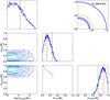 |
Fig. 13 One- and two-dimensional posterior distributions for inferred mass fractions of water log mupper/Mp, mantle mmantle/Mp, and core mcore/Mp for the MRA-SH scenario. The top right panel shows the Rcore/Rp ratio of Gl 486 b (dashed blue with 1σ dashed area) and of the four Solar System telluric planets. Green and red vertical lines denote the Earth and Mars values; comparisons to Mercury and Venus data must be done with caution. Posterior distributions and radii for MR-S and MRA-S scenarios are displayed in Fig. A.2. |
5.3 Prospects for atmospheric characterisation
Here, we present possible atmospheric models of Gl 486 b and discuss whether future observations, especially with Webb, will be able to differentiate between them. One of the key atmosphere parameters that is an input for atmosphere models is the scale height, H. It is the increase in altitude for which the atmospheric pressure decreases by a factor of e (Euler’s number):
 (9)
(9)
where T is the temperature, m is the mean molecular mass, g is the surface gravity, and kB is the Boltzmann constant. In the Solar System, H of the three telluric planets with atmospheres and Titan are defined immediately above the surface where the troposphere is located, and, therefore, T ≈ Tsurf. Above the surface and below the tropopause, rotational turbulence mixes the layers of the atmosphere (the Earth’s tropopause height varies from about 9 km at the poles to 17 km at the equator), and the mean molecular mass of the ‘dry air’ (without water vapour content) remains constant. H is also a key input parameter for the equivalent height of the absorbing atmosphere  which is widely used in exoplanet atmosphere studies (e.g. Nortmann et al. 2018; Orell-Miquel et al. 2022).
The surface temperature, Tsurf, strongly depends on the equilibrium temperature, Teq. In radiative equilibrium, a planet Teq depends on the stellar bolometric luminosity, the planet Bond albedo, and the star-planet separation, through:
 (10)
(10)
where a is the semi-major axis (when e = 0), σ is the Stefan–Boltzmann constant, and є is the atmosphere emissivity. As is customary in the literature, we assumed є = 1.0, by which the whole surface of the planet emits as a black body (if the planet is in radiative equilibrium and there is no heat transfer between both hemispheres, є = 0.25). There are many formal ways of estimating a planet surface temperature, Tsurf, from Teq and the properties of an Earth-like atmosphere. Given the vast amount of uncertainties in the Gl 486 b planet system parameters, we used the simple approach of Houghton (1977), who quantified an atmosphere greenhouse effect with an effective optical thickness, τ :
 (11)
(11)
In the Solar System, τ ≈ 0.09, 0.94, and 160 for Mars, the Earth, and Venus, respectively (Table 10). As a result, the minimum Tsurf of a rocky planet is the Teq for ABond = 1 (total reflectance) and τ = 0 (total transparent atmosphere; i.e. no atmosphere), while the maximum Tsurf is attained for Earth’s open ocean or C-type asteroid-like albedos (ABond = 0.03–0.10) and Venus-like optical thickness (the greatest known to date). Since ABond is bolometric, it depends on the wavelength of the incident flux and, therefore, the spectral type of the stellar host. In planets around M dwarfs, the spectral energy distributions that peak at the red optical-near-infrared boundary (Cifuentes et al. 2020 and references therein), large values of ABond are unlikely because of the expected strong atmospheric absorption at these wavelengths, such as the telluric absorption bands in Fig. 7 (e.g. Irvine & Pollack 1968; Kieffer et al. 1977; Sudarsky et al. 2000; Rogers et al. 2009). This unlikeliness of large values, together with a simpler computation and the smooth dependence Teq ∝ (1 − ABond)1/4, explains why many works assume ABond = 0 for exoplanets around M dwarfs.
In the left panel of Fig. 14, we plot the isotherms of Tsurf for different values of ABond from 0.0 to 1.0 and τ from 0.1 to 100. A priori and without any actual observation of the atmosphere of Gl 486 b, we can only hypothesise its approximate location in the bottom left quadrant of the diagram, with most probable albedos being less than 0.4 (~1.3ABond,⊕) and optical thickness values less than 3 (~3.2τ⊕). With the determined and a and most ABond-τ combinations, Tsurf is below the critical value at 880 K, above which surface rocks can be partially devolatilised (Mansfield et al. 2019). Even with the highest ABond and lowest t, Gl 486 b would never be habitable according to the standard definition (Kasting et al. 1993; Kopparapu et al. 2013). However, a better Teq and Tsurf determination, perhaps from multi-dimensional climate models, would help in future atmospheric retrievals such as the ones presented below (e.g. Fauchez et al. 2020 and references therein).
In the right panel of Fig. 14, we plot lines of constant mean molecular mass as a function of Tsurf for different atmosphere compositions, with mean molecular masses from ~1.3u (90% H, 10% He) to ~44.0u (pure carbon dioxide). Depending on the actual Tsutf and atmospheric composition, Gl 486 b H can vary by almost two orders of magnitude from Earth’s H⊕ ≈ 8.5 km to up to 400 km of a primordial hydrogen and helium atmosphere.
As summarised by Table 11, the Gl 486 system has already been scheduled for future observations with space missions such as TESS, Webb, and Hubble (besides XMM-Newton and Chandra). Only the observations with Webb, namely low-resolution spectroscopy in the near- and mid-infrared with NIR-Spec and MIRI, are aimed at investigating the atmosphere of the planet, while the other observations are equally necessary but focused on quantifying the stellar coronal activity of the host star.
We quantitatively assessed the suitability of Gl 486 b for atmospheric characterisation with both NIRSpec and MIRI. However, before doing so, one must assess the actual presence of an atmosphere surrounding the planet. In the absence of high-quality X-ray and ultraviolet data, we used the Lx and LEUV upper limits in Table 2 to compute maximum values of the XUV flux that arrives at Gl 486 b and the subsequent current atmosphere mass-loss rate, given at the bottom of Table 9. To compute FXUV and  , we used the procedures of Sanz-Forcada et al. (2011). Although the mass-loss rate during the first stages of evolution of the host star was necessarily greater (Ribas et al. 2005; Kubyshkina et al. 2018), the tabulated upper limit of present-day
  translates into 0.07 M⊕ Ga−1, which is comparable to or relatively low in comparison with many transiting exoplanets with atmospheres investigated to date (e.g. K2-100b with more than 0.5 M⊕ Ga−1, Barragán et al. 2019; TOI-849b with 0.95 M⊕ Ga−1, Armstrong et al. 2020; Gl 436 b with 0.019 M⊕ Ga-1, Sanz-Forcada et al. 2011; Villarreal D’Angelo et al. 2021; Foster et al. 2022; see Fig. 11 of the latter authors for a population study). Therefore, available XUV data suggest that Gl 486 b may still retain an atmosphere.
For the quantitative assessment of the Gl 486b suitability for atmospheric characterisation, we synthesised a collection of atmospheric spectra with five scenarios, all of them consistent with the planet interior characterisation in Sect. 5.2. These are (i) optimistic – a substantial H/He gaseous envelope with a relatively low mean molecular weight (i.e. solar abundances); (ii) feasible – an H/He gaseous envelope with enhanced metallicity (i.e. 100× solar abundances); (iii) realistic and compatible with our interior MRA-SH scenario model – an H2O-dominated atmosphere; (iv) realistic – a CO2-dominated atmosphere; and (v) pessimistic – bare rock with a tenuous atmosphere.
The atmospheric composition, spectra, and uncertainties were calculated using the photo-chemical model ChemKM (Molaverdikhani et al. 2019a,b, 2020), the radiative transfer code petitRADTRANS (Mollière et al. 2019), and the community tool Pandexo for transiting exoplanet science with Webb and Hubble (Batalha et al. 2017). The system parameters, including planet mass, radius, equilibrium temperature, transit duration, stellar mass, radius, magnitude, and metallicity were taken from Tables 2 and 9.
The resulting synthetic transmission spectra for the optimistic scenario (i) show strong absorption features due to H2O, CH4, and CO2 over the wavelength range of 0.8–10 µm, as shown in the top panel of Fig. 15. The spectral signature amplitudes are of the order of 50–100 ppm when no haze is assumed. However, haze opacity contribution obscures the mentioned absorption features (e.g. Fortney et al. 2005; Kreidberg et al. 2014; Nowak et al. 2020; Trifonov et al. 2021), particularly at short wavelengths. Here, haze is defined the same way as in Nowak et al. (2020), who included C8H6, C8H7, C10H3, C12H3, C12H10, C14H3, C2H4N, C2H3N2, C3H6N, C4H3N2, C4H8N, C5HN, C5H3N, C5H4N, C5H6N, C9H6N, C3H3O, C3H5O, C3H7O, and C4H6O. All these precursor molecules that represent the haze particles are collectively called soot or haze (e.g. Lavvas & Koskinen 2017).
An increase in the atmospheric metallicity (i.e. scenario ii) enhances this obscuration effect both due to a higher mean molecular weight and a higher haze production rate, as illustrated by the dampened spectral features in the second panel of Fig. 15. Such an H/He gaseous envelope with enhanced metallicity might be a feasible scenario in a rocky planet, for instance, due to the resupply of hydrogen from magma outgassing (Chachan & Stevenson 2018; Kite et al. 2019; Kite & Barnett 2020). Both scenarios (i.e. optimistic, i, and feasible, ii) would be distinguishable with only two transits observed by Webb over a wide range of wavelengths if the atmosphere were haze-free. However, given that a hazy atmosphere for this class of planets has been proposed to be likely (e.g. Gao et al. 2018; Yu et al. 2021), using only NIRSpec/G395H may require more than two transits to differentiate between different (solar or enhanced metallicity) H/He-dominated scenarios.
Terrestrial planets in the Solar System and models of evolution of exoplanetary atmospheres suggest that small planets are less likely to maintain an H-dominated atmosphere (e.g. Gao et al. 2015; Woitke et al. 2021). For example, Ortenzi et al. (2020) showed that for a ~ 3 M⊕ planet such as Gl 486 b, a very efficient H2O outgassing, and hence an H2O dominated atmosphere, is a more likely scenario. Therefore, in our realistic scenario iii, we simulated such an atmosphere based on the outcome of our planet interior MRA-SH model. We assumed an isothermal atmosphere with a temperature equal to the equilibrium temperature of the planet up to 100 hPa (0.1 bar), which roughly marks the tropopause temperature. Then, the temperature profile follows an adiabat. The resulting spectrum is illustrated in the third panel of Fig. 15, with water features reduced in amplitude by a factor of a few compared with the enhanced-metallicity H/He-dominated scenario (ii), which is mainly due to a higher mean molecular weight. The uncertainties shown for ten transits suggest that a steam atmosphere would be detectable under these circumstances, although haze and clouds might obscure water features significantly.
In spite of the fact that an H2O-dominated atmosphere is a more likely scenario according to Ortenzi et al. (2020), a CO2-dominated atmosphere cannot be ruled out in the case of a very dry and oxidised mantle. Moreover, examples in the Solar System, such as Venus and Mars, support such a possibility. Hence, we also assumed a CO2-dominated atmosphere for Gl 486 b to synthetise another realistic spectrum, namely scenario iv. Such an atmosphere could have evolved from an initial secondary atmospheric composition (e.g. H2O, CO, and CO2), as hinted by carbonaceous chondrite outgassing measurements (Thompson et al. 2021). In this scenario, a higher mean molecular weight results in a smaller atmospheric scale height and, therefore, smaller spectral features. This effect is shown in the fourth panel of Fig. 15, where a total of 20 transits were employed to achieve a reasonable S/N for the detection of CO2 features on the order of 5–10 ppm. The number of required transits would increase even more if haze contribution, such as a Venusian atmosphere, were also considered. A way to overcome this issue is to observe this planet in emission.
The day-side temperature of Gl 486 b is expected to be cold enough to maintain an atmosphere, but hot enough to be suitable for emission spectroscopy. The bottom panel of Fig. 15 illustrates a synthetic Webb emission spectrum of a realistic CO2-dominated atmosphere. The relative flux remains below 20 ppm with slight spectral modulations below 5 µm. However, it increases to 100-150 ppm at longer wavelengths, where MIRI/LRS spans its coverage. Uncertainty estimations suggest that the spectral features, particularly around 9 µm, should be detectable with only two eclipses. Therefore, both transmission and emission spectroscopy are necessary to characterise the atmosphere of Gl 486b over different scenarios. The two eclipses of GO 1743 (MIRI/LRS) and the two transits GO 1981 (NIRSpec/G395H) programmed for Webb cycle 1 (Table 11) will certainly shed light on the composition and structure of the atmosphere of the exoearth.
Still, the pessimistic scenario (v) of a bare rock with a tenuous atmosphere would be out of reach for Webb instruments. Therefore, we examined such a scenario for two cases by employing ground-based high-resolution spectrographs, such as CARMENES or MAROON-X. In the first case, we assumed a Mars-like surface pressure of 1 hPa (10−3 bar). With such a pressure, the atmosphere is likely to be thermalised at the surface and, therefore, we used the Teq for null albedo of about 700 K. Welbanks et al. (2019) conducted a homogeneous retrieval of sodium abundance for 19 exoplanets and found that about half of these planets show an abundance of 10−9 or non-detection. Hence, the synthetic spectrum around the D2 and D1 sodium doublet, Na I, 125889.95,5895.92 Å, is shown in the top panel of Fig. 16 for a Mars-like surface pressure and an Na abundance of 10−9. The estimated uncertainties for CARMENES over two transits are much larger than the signals that, hence, remain undetected. The Na D2 and D1 doublet is one of the strongest planetary lines and, thus, other spectral lines are expected to face a similar fate with a tenuous, thermalised atmosphere.
The second case of a bare rock is by assuming an even more tenuous atmosphere. Although this may seem contradictory at first glance, a lower surface pressure might help to heat up the surface species to more than 10 000 K through non-thermal processes, such as surface sputtering by ions (e.g. Bida et al. 2000). In this case, we assumed a surface pressure of around 0.001 hPa (10−6 bar, still several magnitudes higher than that of Mercury), a temperature of 10 000 K, and the same Na abundance of 10−9. We estimated the absorption excess of the Na D2 line, illustrated by the middle panel of Fig. 16, at around 1%, which is large enough for an instrument such as CARMENES to resolve the line. The bottom panel of Fig. 16 illustrates the same atmospheric scenario observed through 20 transits. The characterisation of such atmospheres would be a more suitable task for facilities with more light-gathering power, such as ESPRESSO at the 8.4m Very Large Telescope or ANDES at the 39 m Extremely Large Telescope. Moreover, molecular formation under such conditions is unlikely, but atomic and ionic species that do not have strong resolved lines might still be detectable with the cross-correlation technique (e.g. Snellen et al. 2010).
We estimate that two transits would suffice to meet S/N = 5 for the realistic (CO2-dominated) atmosphere model, while a single transit would be enough for the other four models, namely the optimistic (H/He and 1 × [Fe/H]⊙), feasible (H/He and 100 × [Fe/H]⊙), interior-compatible-realistic (H2O-dominated), and pessimistic (emission) models. However, the definition of the S/N becomes arbitrary and model dependent when dealing with low-resolution spectra over a wide wavelength range. For example, the S/N calculated directly by dividing signals by their corresponding noises (uncertainties) for each spectral bin would not ensure the differentiation of atmospheric scenarios. Therefore, we defined back-of-the-envelope baseline models (a flat line for transmission, the ratio of two black body functions for emission), removed them from the signals, and used the residuals to estimate the sum of all S/Ns for all spectral bins and within each instrument range. As a result, our estimations must be used with care. Instead of reporting S/N, we suggest comparing the models and choosing the best one according to their log evidence.
Altogether, Gl 486 b provides an exceptional opportunity to characterise the atmosphere of an exoearth. However, our analysis shows synergistically planned observations between ground-based facilities and Webb instruments would be needed to achieve that goal.
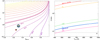 |
Fig. 14 Basic atmospheric parameters of Gl 486 b. Left: Surface temperature as a function of Bond albedo and atmospheric optical thickness, from 500 K to 2000 K in steps of 100 K. The coolest isotherms are labelled. The isotherm of 880 K, at which silicon-based surfaces melt, is drawn with a thick line. The Earth and Mars are indicated as a reference (but their Tsurf do not correspond to those of Gl 486 b because of different L* and a; see Eq. (10)). Venus, with τ ≈ 160, is out of limits. Left: Scale height as a function of surface temperature and mean molecular mass for different atmospheric compositions. From top to bottom: 90% H + 10% He (1.31 u, red), H2 (2.02 u, orange), H2O (18.0 u, green), N2 (28.0 u, cyan), Earth dry air (29.0 u, blue), CO2 (44.0 u, magenta). The dashed horizontal line indicates the Earth scale height (Hφ = 8.5 km), while the grey shaded area marks the surface temperature for rock volatilisation (Tsurf ≳ 880 K). |
Forthcoming space observations of Gl 486 and Gl 486 b in the optical and infrared.
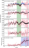 |
Fig. 15 Synthetic Webb atmospheric spectra of Gl 486 b. From top to bottom: Transmission spectra under optimistic (i), feasible (ii), realistic and interior-compatible (iii), and realistic (iv) scenarios, and emission spectrum for the realistic (iv) scenario. Red circles with estimated uncertainties are shown for different numbers of transits and eclipses as stated in the panels, with Webb NIRISS/SOSS, NIRSpec/G395H, and MIRI/LRS configurations. Black and blue lines represent clear (i.e. no haze opacity contribution) and hazy atmospheres, respectively. There is no hazy atmosphere in the realistic scenarios. NIRSpec/G395H and MIRI/LRS (Table 11) wavelength coverages are highlighted by green and blue shades, respectively. |
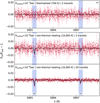 |
Fig. 16 Synthetic CARMENES atmospheric spectra of Gl 486 b. Transmission spectra around the Na i D1 and D2 doublet under the pessimistic scenario (iv: a bare rock with a tenuous atmosphere) for a thermalised atmosphere and two transits (top), and for an exosphere with non-thermal heating and two transits (middle) and 20 transits (bottom). |
6 Conclusions
At a distance of only 8.1 pc, Gl 486 b is the third closest transiting planet to the Sun and presents an important addition to the demographics of known transiting rocky planets. The relatively bright, very weakly active, M-dwarf host star, its visibility from both Earth hemispheres, and the short orbital period and warm expected surface temperature make this planet one of the best targets for planet atmosphere emission and transit spectroscopy with Webb and future ground-based extremely large telescopes.
In this work, we slightly improve the precision and accuracy of the planet mass and radius determination, with which we develop different planet interior and atmosphere scenarios. Except for the eccentricity, of which the upper limit is set at 0.025, the improvement of most parameters with respect to what Trifonov et al. (2021) tabulated is slim. However, there are a few differences with respect to previous work that make this analysis unique. Instead of estimating the stellar radius from luminosity and model-dependent spectral synthesis, we directly measured the angular radius of the planet host star with MIRC-X at the CHARA Array. We reduced the input data error contribution by gathering extremely precise RV data collected by CARMENES and MAROON-X and transit data obtained by TESS and, presented here for the first time, CHEOPS. The selected joint RV and transit fit model, 1pl+GP, was supported by an independent photometric monitoring with small and medium-size telescopes for determining the stellar rotation period, which turned to be shorter than previously reported and of very low amplitude. The additional errors in planet radius and mass introduced by the transit and RV data with respect to the uncertainties in star radius and mass were just 0.3% and 0.4%, respectively, possibly at the limit of what is technically possible nowadays.
As a novelty in M dwarfs, we determined Mg, Si, V, Fe, Rb, Sr, and Zr abundances of the stellar host, which constrained two of the three considered planet interior scenarios. We also considered different planet atmosphere scenarios and their detectability with forthcoming Webb observations with NIRSpec and MIRI after taking into account different possibilities on composition and planet surface temperature and pressure.
In the most probable combination of scenarios, Gl 486 b is a warm, Earth-like planet of R ~ 1.343 Re and M ~ 3.00M⊕ with a relatively low-mass and metallic core surrounded by a silicate mantle with dissolved water and an upper layer probably composed of a mixture of water steam and carbon dioxide. Now it is time to do comparative planetology and investigate topics on solid grounds that were provocative until very recently. For example, if there is a liquid outer core, and because of the fast, tidally locked planet rotation of 1.47 days, there may be a strong magnetic field that protects the Gl 486 b atmosphere from stellar erosion (Scalo et al. 2007); or, if a thick atmosphere is indeed preserved, there may be jet streams that transport heat from the illuminated to the dark hemisphere as in hot Jupiters (Showman & Polvani 2011). These and other novel studies based on the results presented here, such as simultaneously deriving stellar and planetary mass and radius using interferometry and probability density functions (Crida et al. 2018) or constraining the oxygen fugacity of the planet (Doyle et al. 2019), will soon be available.
Acknowledgements
We thank the reviewer for helpful comments, Kate Isaak for her support on CHEOPS observations, Mahmoudreza Oshagh for her preliminary transit-time variation analysis, David Ciardi for helpful comments on deep adaptive optics imaging, Vera M. Passegger for her Mg i fit, Sandra V. Jeffers for comments on stellar activity, and Joel Hartman, Greg W. Henry, Jonathan Irwin, and Chris G. Tinney for their information on HATNet, TSU, MEarth, and APT photometric data. CHEOPS is an ESA mission in partnership with Switzerland with important contributions to the payload and the ground segment from Austria, Belgium, France, Germany, Hungary, Italy, Portugal, Spain, Sweden and the United Kingdom. The development of the MAROON-X spectrograph was funded by the David and Lucile Packard Foundation, the Heising-Simons Foundation, the Gemini Observatory, and the University of Chicago. This work was enabled by observations made from the Gemini North telescope, located within the Maunakea Science Reserve and adjacent to the summit of Maunakea. We are grateful for the privilege of observing the Universe from a place that is unique in both its astronomical quality and its cultural significance. CARMENES is an instrument at the Centro Astronómico Hispano en Andalucía (CAHA) at Calar Alto (Almería, Spain), operated jointly by the Junta de Andalucía and the Instituto de Astrofísica de Andalucía (CSIC). CARMENES was funded by the Max-Planck-Gesellschaft (MPG), the Consejo Superior de Investigaciones Científicas (CSIC), the Ministerio de Economía y Competitividad (MINECO) and the European Regional Development Fund (ERDF) through projects FICTS-2011-02, ICTS-2017-07-CAHA-4, and CAHA16-CE-3978, and the members of the CARMENES Consortium (Max-Planck-Institut für Astronomie, Instituto de Astrofísica de Andalucía, Landessternwarte Königstuhl, Institut de Ciències de l’Espai, Institut für Astrophysik Göttingen, Universidad Complutense de Madrid, Thüringer Landessternwarte Tautenburg, Instituto de Astrofísica de Canarias, Hamburger Sternwarte, Centro de Astrobiología and Centro Astronómico Hispano-Alemán), with additional contributions by the MINECO, the Deutsche Forschungsgemeinschaft (DFG) through the Major Research Instrumentation Programme and Research Unit FOR2544 “Blue Planets around Red Stars”, the Klaus Tschira Stiftung, the states of Baden-Württemberg and Niedersachsen, and by the Junta de Andalucía. This work is based upon observations obtained with the Georgia State University (GSU) Center for High Angular Resolution Astronomy Array at Mount Wilson Observatory. The CHARA Array is supported by the National Science Foundation under Grant No. AST-1636624 and AST-2034336. Institutional support has been provided from the GSU College of Arts and Sciences and the GSU Office of the Vice President for Research and Economic Development. We would like to recognise the observing team, scientists, and support staff at the CHARA Array. Observation time for this work was generously allocated via discretionary time from CHARA Array director Theo ten Brumelaar and via NOIRLab community access program (proposals 2021A-0247 and 2021A-0141). MIRC-X received funding from the European Research Council (ERC) under the European Union’s Horizon 2020 research and innovation program (Grant No. 639889), as well as from NASA (XRP NNX16AD43G) and NSF (AST 1909165). Data were partly collected with the 90 cm telescope at the Observatorio de Sierra Nevada operated by the Instituto de Astrofífica de Andalucía (IAA-CSIC). This work made use of observations from the Las Cumbres Observatory Global Telescope network. LCOGT observations were partially acquired via program number TAU2021A-015 of the Wise Observatory, Tel-Aviv University, Israel. We acknowledge financial support from the Agencia Estatal de Investigación of the Ministerio de Ciencia, Innovación y Universidades and the ERDF through projects PID2019-109522GB-C5[1:4], PID2019-107061GB-C64, PID2019-110689RB-100, PGC2018-095317-B-C21, PGC2018-102108-B-I00, and the Centre of Excellence “Severo Ochoa” and “María de Maeztu” awards to the Instituto de Astrofísica de Canarias (CEX2019-000920-S), Instituto de Astrofísica de Andalucía (SEV-2017-0709), and Centro de Astrobiología (MDM-2017-0737), DFG through FOR2544 (KU 3625/2-1) and Germany’s Excellence Strategy to the Excellence Cluster ORIGINS (EXC-2094 - 390783311), European Research Council (Starting Grant 639889), Bulgarian National Science Fund through VIHREN-2021 (KP-06-DB/5), Schweizerischer Nationalfonds zur Förderung der wissenschaftlichen Forschung / Fonds national suisse de la recherche scientifique (PZ00P2_174028), United Kingdom Science Technology and Facilities Council (630008203), NASA (80NSSC22K0117), National Science Foundation (2108465 and Graduate Research Fellowship DGE 1746045), Princeton University through the Henry Norris Russell Fellowship, Universidad La Laguna through the Margarita Salas Fellowship from the Spanish Ministerio de Universidades and under the EU Next Generation funds (UNI/551/2021-May 26), and the Generalitat de Catalunya (CERCA programme). We used the NASA Exoplanet Archive, which is operated by the California Institute of Technology, under contract with the National Aeronautics and Space Administration under the Exoplanet Exploration Program, and Uncertainties, a Python package for calculations with uncertainties developed by E. O. Lebigot (https://pythonhosted.org/uncertainties).
Appendix A Short tables and diagrams
Published heliocentric radial velocities of Gl 486a.
Multiband photometry of Gl 486a.
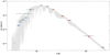 |
Fig. A.1 Spectral energy distribution of Gl 486. The apparent fluxes (coloured filled circles) are imposed on a BT-Settl CIFIST spectrum (grey; Teff = 3200 K and log g = 5.5). The modelled fluxes are depicted as black empty circles. The photometric datum in u’ (purple cross) was not considered for integrating the bolometric luminosity. Horizontal bars represent the effective widths of the bandpasses (equivalent to the horizontal size of a rectangle with height equal to maximum transmission and with the same area that the one covered by the filter transmission curve), while vertical bars (visible only for relatively large values) represent the flux uncertainty derived from the magnitude and parallax errors. See details in Cifuentes et al. (2020). |
Published effective temperatures of Gl 486a.
Published relative iron abundances of Gl 486.
Emission measure distribution of Gl 486.
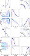 |
Fig. A.2 Same as Fig. 13 but for the MR-S (baseline, top) and MR-SA (baseline plus relative stellar abundance constraints, bottom) planet interior scenarios. |
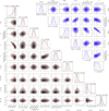 |
Fig. A.3 Nested samples distribution of fitted (black) and derived (blue) parameters of Gl 486 b with CARMENES and MAROON-X RV data and CHEOPS and TESS light curves. The position of the median from the posterior is marked with red grid lines. The contours on the 2D panels represent the 1σ, 2σ, and 3σ confidence levels of the overall posterior samples. The top (black) and bottom (blue) panels of every column represent the 1D histogram distribution of each parameter. |
Priors and posteriors of the joint transit and RV fit of Gl 486a.
CARMENES and MAROON-X Red and Blue RVs of Gl486.
Appendix B Sources of error and propagation of uncertainty
Appendix B.1 Planet radius and mass
Gl 486 b is among the smallest and least massive transiting planets, and among the ones with the smallest relative uncertainties in both radius and, especially, mass. However, there are even smaller and less massive planets (e.g. in the TRAPPIST-1 system), which have smaller reported relative uncertainties. Planets with very small reported uncertainties orbit eclipsing binary stars (with precise and accurate R* and M* determinations) or suffer from incorrect error propagation. This is illustrated in the δRp-Rp and δMp-Mp diagrams in Fig. B.1.
With  in Gl 486 b, we reached the 10% precision boundary on the core-to-mantle ratio of a telluric exoplanet. Breaking this precision boundary will give rise to planet internal composition studies not done before. However, in order to obtain a precision better than 10% on the core-to-mantle ratio of a terrestrial exoplanet (actually, the “core radius fraction”), it is required a measurement of the mass better than 11% and a measurement on the radius better than 3% (Suissa et al. 2018). The approximate uncertainty ratio of three-to-one is also applied to the planet bulk density. From the sphere density formula, the uncertainty in planet radius Rp contributes three times more to the final error of planet bulk density ρp than the uncertainty in planet mass Mp:
 (B.1)
(B.1)

For Gl 486b, the measured relative uncertainties in planet radius and mass translate into a bulk density relative uncertainty of 9.3%, which allowed to determine its internal composition and structure. In our case, we fitted the r1 and r2 parameters, from which we derived the radius ratio, p, and impact parameter, b (Espinoza et al. 2019). The planet radius comes from the simple definition of p:
 (B.3)
(B.3)
and its uncertainty is, therefore:
 (B.4)
(B.4)
As a result, the relative uncertainty in Rp can never be smaller than that in R*. For Gl 486 b,  , the relative error in p is very small, and, therefore, δRp/Rp ≈ δR*/R*. Actually, from Sect. 4.5, the derived planet radius is
  , which represents a relative uncertainty of 4.7% and is very similar to the relative uncertainty of the stellar radius, at 4.5%. The small difference of 0.2% through the p parameter is mostly due to the quality of the TESS and CHEOPS transit data.
The derivation of the relative uncertainty in Mp is, a priori, more complicated and highly non-linear. From the definition of the RV semi-amplitude:
 (B.5)
(B.5)
it can be deduced the following:
 (B.6)
(B.6)
 (B.7)
(B.7)
where P, K, and e are fitted parameters, i is a derived parameter, and M* is an input parameter. Nevertheless, in most cases it happens that M* >> Mp. For example, for Gl 486 b, the ratio between planet and star masses is about 2.7 × 10⁻⁵, which justifies the following approximation:
 (B.8)
(B.8)
As a result, the uncertainty in planet mass becomes:
 (B.9)
(B.9)
When the uncertainty in M* dominates the global error contribution with respect to P, K, i, and e, as in the case of typical observations with CARMENES+MAROON-X or ESPRESSO, the latter equation remains just:
 (B.10)
From Sect. 4.5, the derived planet mass is  , which represents a relative uncertainty of 4.2%, and is about two thirds of the relative uncertainty of the stellar mass, at 5.6%. The small difference of 0.4% through the P, K, and i (and e) parameters is, in this case, mostly due to the quality of the CARMENES and MAROON-X RV data, some of them with sub-metre-per-second precision.
Fig. B.2 illustrates these computations. The majority of confirmed planets fall on or above the 1:1 radius relative error ratio in the δRp/Rp vs. δR*/R* diagram (left panel) and on or above the 2:3 mass relative error ratio in the δMp/Mp vs. δM*/M* diagram. Gl 486b, displayed in both panels of Fig. B.2 with a black filled star, has radius and mass determinations near, but slightly above, the empirical boundaries at δRp/Rp ~ δR*/R* and δMp/Mp ~ 2δM*/3M*. The outliers with δRp/Rp << δR*/R* (Wendelstein 1b and 2 b, Obermeier et al. 2020; CoRoT-27 b, Parviainen et al. 2014; and Kepler-30 b, c and d, Sanchís-Ojeda et al. 2012) and δMp/Mp << δM*/M* (BD+46 2629Ab = Kepler-13b, Esteves et al. 2015; and LTT 9779 b, Jenkins et al. 2020) suffered again from incorrect error propagation. For example, Sanchís-Ojeda et al. (2012) tabulated 3.9 ± 0.2, 12.3 ± 0.4, and 8.8 ± 0.5R⊕ for planets b, c, and d in the Kepler-30 system but, from their R* and Δ = (Rv/R*)2 and the SI values for R⊙ and R⊕, we determined instead 4.21 ± 0.54, 13.2 ± 1.7, and 9.4 ± 1.2R⊕, respectively28.
 |
Fig. B.1 Uncertainty in radius versus radius (left) and uncertainty in mass versus mass (right) of all transiting exoplanets with mass determination (from RV or transit time variations). The symbol colour denotes the stellar host effective temperature, while the symbol size is proportional to mass and radius, respectively. Diagonal dashed lines indicate lines of constant relative uncertainty (1, 2, 5, 10, 20, 50%). Gl 486 b is marked with a black star in both panels. Only in the right panel, the grey vertical dotted line marks the deuterium burning mass limit. The planets with δRp/Rp ratios less than 1 % (left panel) are Kepler-16 b |

Appendix B.2 Stellar radius and mass
While we break by a wide margin the planet mass boundary of Suissa et al. (2018) for internal composition studies at 11%, we get very close to break the planet radius boundary at 3%. The space photometry and RV spectroscopy add only 0.2% and 0.4% extra uncertainty to the fit, respectively, so we are in the case of planet parameters limited by the stellar parameter uncertainties, especially the stellar radius. In our case, this problem is partially alleviated by our accurate interferometric measurements. We analyse below the sources of limiting errors in determining stellar parameters, apart from improvements in RV and transit photometry precision and systematics correction.
We computed the stellar mass M* from the stellar radius R* with the linear mass-radius relation of Schweitzer et al. (2019):
 (B.11)
where α = −0.0240 ± 0.0076 M⊙,  , and R* is expressed in solar units (Sect. 2 - we use α, β instead of a, b as in the original work for avoiding confusion with p, b Juliet parameters). From this relation, the uncertainty in stellar mass is, therefore:
 (B.12)
In our case, we determined the stellar radius with near-infrared interferometric measurements with MIRC-X at the CHARA Array (Sects. 3.3 and 4.1). In particular, R*,interf is a simple function of the stellar angular diameter, θ, and the parallax, ϖ, or, alternative, the parallactic distance, d:
 (B.13)
and the corresponding relative uncertainty is:
 (B.14)
To sum up, the uncertainty in stellar mass from an interferometric stellar radius becomes:
 (B.15)
In most cases, especially for stars within 10 pc of the Sun such as Gl 486, the uncertainty in distance is much smaller than those in angular diameter and slope of the mass-radius linear relation. In Sect. 3.3 we determined a stellar limb-darkened disc diameter θLDd = 0.390 ± 0.018 mas, which error propagated from the scatter of the squared visibility, V2, as a function of spatial frequency, B′/λ, and the uncertainties in all fit parameters (i.e.,  . The uncertainty inθLDd, of ~4.5%, is about three times larger that of β, of ~1.6%, and almost 20 times larger than that of d, of barely ~0.3%. As a result,
δR*,interf/R*,interf ≈ δθLDD/θLDD, which agrees with the stellar radius relative uncertainty of ~4.5% as in Table 2. After including the α and β contributing errors, the stellar mass relative uncertainty becomes the nominal 5.6%.
 |
Fig. B.2 Relative errors in star (X axis) and planet (Y axis) radius (left) and mass (right). Grey open circles: all exoplanet candidates in exoplanets.org. Coloured filled symbols: planets with both mass and radius determination (from RV and transits or transit time variations): the symbol colour denotes the stellar host effective temperature, while the symbol size is log-proportional to the planet radius (left) and mass (right). Black star: Gl 486 system. Solid diagonal lines: 1:1 radius (left:) and 2:3 mass (right:) relative error ratios. Only in the right panel, we also plot a dashed diagonal line at the 1:1 mass relative error ratio, which corresponds to microlensing planets. |
When there is no interferometric determination of the stellar radius, Schweitzer et al. (2019) proposed deriving R* through the Stefan-Boltzmann law from bolometric luminosity and an equilibrium temperature derived from spectral synthesis:
 (B.16)
and its uncertainty is, thus:
 (B.17)
As a result, the uncertainty in Teff to R*,synth contributes four times that in L*. In turn, the uncertainty in luminosity, which is computed from the distance and observed flux after integrating the stellar spectral energy distribution from the blue optical to the mid infrared (L* = 4πd2Fobs), is relatively small for nearby stars with precise Gaia EDR3 parallactic distance and a wealth of well-calibrated multiband photometry:
 (B.18)
As a result, the error in the determination of R*,synth is dominated by that of Teff, which can be 50–200 K in M dwarfs (Passegger et al. 2022).
The following equation summarises all the contributions to the uncertainty in stellar mass in absence of interferometric observations:
 (B.19)
There are different ways of reducing the uncertainties in stellar radius and mass:
Acquiring more and better interferometric data. There are, however, technical and logistics limitations to this, as observing at wide baselines and dense ranges of spatial frequencies with up to six CHARA Array telescopes or any other interferometer is time consuming. Besides, although the scenario is not as serious as for the AstroLAB site, Gl 486 culminates at an altitude of only ~65.5 deg as seen from Mount Wilson.
If there are no interferometric data, improving the Teff determination. We refer to Marfil et al. (2021) and Passegger et al. (2022) for recent and exhaustive comparisons of methodologies for determining Teff of M dwarfs.
Improving the mass-radius relation. TESS is discovering new detached, M-dwarf, eclipsing binaries (e.g., Lendl et al. 2020; Prša et al. 2022), some of them with relatively large orbital periods that lack enhanced magnetic activity and, thus, stellar inflation as in the ones with the shortest periods (Kraus et al. 2011). Special attention must also be given to not including in the fit young eclipsing binaries in stellar kinematic groups that are still on the Hayashi track (Schweitzer et al. 2019).
Measuring a more precise bolometric observed flux. Differences between Fobs computed by us with VOSA or by other teams are in the details, such as origin of the photometry, template choice, handling of zero-points and transmission profiles (Cifuentes et al. 2020). It is however difficult to get better than 1.1% as measured by us because, even if the photometry has tiny errors and the spectral templates are perfect, almost all photometry is calibrated to the same set of standard stars. Those standards only have their true Fobs measured to about 1–2% based on STIS/Hubble Space Telescope spectro-photometric calibrations (Bohlin & Gilliland 2004; Bohlin 2007; Maíz Apellániz & Weiler 2018). Webb and its extended wavelength range towards the near- and mid-infrared can soon be used for improving the bolometric flux of standard stars.
Improving the parallactic distance determination. There is strong evidence that Gaia EDR3 parallax errors are underestimated, especially for bright stars (e.g., Luri et al. 2018; El-Badry et al. 2021; Fabricius et al. 2021; Maíz Apellániz 2022). At G - 10 mag the underestimation can be up to 60%. Since Gaia DR3 parallactic distances will be those already published in EDR3, we will have to wait for DR429 for having uncertainties so small that they will in general be negligible with respect to the errors in other parameters.
Appendix B.3 Element abundances
Slightly different values of A(X) and, therefore, [X/H] can be obtained if other input Teff are used. Different Teff at a fixed Lbol translates into distinct R* and, therefore, M*, Rp, and Mp. However, as discussed in Sect. 2, our Teff from our interferometric radius and bolometric luminosity matches most literature values (Table A.3). The abundances and, therefore, the planet interior models, are also sensitive in a lower degree to the used log g and [Fe/H] values. While the iron abundances of Marfil et al. (2021) seem to be the most reliable ones published to date in M dwarfs (Passegger et al. 2022), their surface gravities are a matter of concern. For example, the Gl 486 surface gravity from our interferometric radius and the mass-radius relation of Schweitzer et al. (2019) is log g ≈ 5.4 dex, which contrasts log gspec = 4.82 ± 0.12 dex from Marfil et al. (2021). Following Passegger et al. (2022), “further in-depth investigations of the employed methods [to determine effective temperatures, surface gravities, and metallicities in M dwarfs] would be necessary in order to identify and correct for the discrepancies that remain”. In any case, the Fe, Mg, and Si abundances derived by us, which are solar within generous uncertainties, can be applicable to current and future planet interior structure and composition models.
References
- Abia, C., Tabernero, H. M., Korotin, S. A., et al. 2020, A&A, 642, A227 [NASA ADS] [CrossRef] [EDP Sciences] [Google Scholar]
- Abia, C., de Laverny, P., Korotin, S., et al. 2021, A&A, 648, A107 [NASA ADS] [CrossRef] [EDP Sciences] [Google Scholar]
- Acuña, L., Lopez, T. A., Morel, T., et al. 2022, A&A, 660, A102 [NASA ADS] [CrossRef] [EDP Sciences] [Google Scholar]
- Adibekyan, V., Dorn, C., Sousa, S. G., et al. 2021, Science, 374, 330 [NASA ADS] [CrossRef] [Google Scholar]
- Ahn, C. P., Alexandroff, R., Allende Prieto, C., et al. 2012, ApJS, 203, 21 [Google Scholar]
- Allard, F., Homeier, D., & Freytag, B. 2012, Philosophical Transactions of the Royal Society of London Series A, 370, 2765 [NASA ADS] [Google Scholar]
- Alonso-Floriano, F. J., Morales, J. C., Caballero, J. A., et al. 2015, A&A, 577, A128 [NASA ADS] [CrossRef] [EDP Sciences] [Google Scholar]
- Amado, P. J., Bauer, F. F., Rodríguez López, C., et al. 2021, A&A, 650, A188 [NASA ADS] [CrossRef] [EDP Sciences] [Google Scholar]
- Ammons, S. M., Robinson, S. E., Strader, J., et al. 2006, ApJ, 638, 1004 [NASA ADS] [CrossRef] [Google Scholar]
- Andersen, J. 1991, A&Ar, 3, 91 [NASA ADS] [CrossRef] [Google Scholar]
- Anglada-Escudé, G., Amado, P. J., Barnes, J., et al. 2016, Nature, 536, 437 [Google Scholar]
- Antoniadis-Karnavas, A., Sousa, S. G., Delgado-Mena, E., et al. 2020, A&A, 636, A9 [NASA ADS] [CrossRef] [EDP Sciences] [Google Scholar]
- Anugu, N., Le Bouquin, J.-B., Monnier, J. D., et al. 2020, AJ, 160, 158 [NASA ADS] [CrossRef] [Google Scholar]
- Arenou, F., Luri, X., Babusiaux, C., et al. 2018, A&A, 616, A17 [NASA ADS] [CrossRef] [EDP Sciences] [Google Scholar]
- Armstrong, D. J., Lopez, T. A., Adibekyan, V., et al. 2020, Nature, 583, 39 [Google Scholar]
- Asplund, M., Grevesse, N., Sauval, A. J., & Scott, P. 2009, ARA&A, 47, 481 [NASA ADS] [CrossRef] [Google Scholar]
- Astudillo-Defru, N., Delfosse, X., Bonfils, X., et al. 2017a, A&A, 600, A13 [NASA ADS] [CrossRef] [EDP Sciences] [Google Scholar]
- Astudillo-Defru, N., Forveille, T., Bonfils, X., et al. 2017b, A&A, 602, A88 [NASA ADS] [CrossRef] [EDP Sciences] [Google Scholar]
- Bajgain, S., Ghosh, D. B., & Karki, B. B. 2015, Nature Commun., 6, 8578 [NASA ADS] [CrossRef] [Google Scholar]
- Barabash, S., Fedorov, A., Lundin, R., & Sauvaud, J.-A. 2007, Science, 315, 501 [CrossRef] [Google Scholar]
- Baraffe, I., Chabrier, G., Allard, F., & Hauschildt, P. H. 1998, A&A, 337, 403 [Google Scholar]
- Baroch, D., Morales, J. C., Ribas, I., et al. 2018, A&A, 619, A32 [NASA ADS] [CrossRef] [EDP Sciences] [Google Scholar]
- Baroch, D., Morales, J. C., Ribas, I., et al. 2021, A&A, 653, A49 [NASA ADS] [CrossRef] [EDP Sciences] [Google Scholar]
- Barragán, O., Aigrain, S., Kubyshkina, D., et al. 2019, MNRAS, 490, 698 [Google Scholar]
- Batalha, N. E., Mandell, A., Pontoppidan, K., et al. 2017, PASP, 129, 064501 [Google Scholar]
- Battistini, C., & Bensby, T. 2015, A&A, 577, A9 [NASA ADS] [CrossRef] [EDP Sciences] [Google Scholar]
- Bean, J. L., Seifahrt, A., Hartman, H., et al. 2010, ApJ, 713, 410 [NASA ADS] [CrossRef] [Google Scholar]
- Bellm, E. C., Kulkarni, S. R., Graham, M. J., et al. 2019, PASP, 131, 018002 [Google Scholar]
- Benz, W., Broeg, C., Fortier, A., et al. 2021, Exp. Astron., 51, 109 [Google Scholar]
- Bergemann, M., Hoppe, R., Semenova, E., et al. 2021, MNRAS, 508, 2236 [NASA ADS] [CrossRef] [Google Scholar]
- Berta-Thompson, Z. K., Irwin, J., Charbonneau, D., et al. 2015, Nature, 527, 204 [Google Scholar]
- Bida, T. A., Killen, R. M., & Morgan, T. H. 2000, Nature, 404, 159 [NASA ADS] [CrossRef] [Google Scholar]
- Bidelman, W. P. 1985, ApJS, 59, 197 [Google Scholar]
- Bluhm, P., Pallé, E., Molaverdikhani, K., et al. 2021, A&A, 650, A78 [NASA ADS] [CrossRef] [EDP Sciences] [Google Scholar]
- Bohlin, R. C. 2007, in Astronomical Society of the Pacific Conference Series, The Future of Photometric, Spectrophotometric and Polarimetric Standardization, ed. C. Sterken, 364, 315 [NASA ADS] [Google Scholar]
- Bohlin, R. C., & Gilliland, R. L. 2004, AJ, 127, 3508 [NASA ADS] [CrossRef] [Google Scholar]
- Boisse, I., Bouchy, F., Hébrard, G., et al. 2011, A&A, 528, A4 [NASA ADS] [CrossRef] [EDP Sciences] [Google Scholar]
- Bonfils, X., Mayor, M., Delfosse, X., et al. 2007, A&A, 474, 293 [NASA ADS] [CrossRef] [EDP Sciences] [Google Scholar]
- Bonfils, X., Delfosse, X., Udry, S., et al. 2013, A&A, 549, A109 [NASA ADS] [CrossRef] [EDP Sciences] [Google Scholar]
- Boro Saikia, S., Marvin, C. J., Jeffers, S. V., et al. 2018, A&A, 616, A108 [NASA ADS] [CrossRef] [EDP Sciences] [Google Scholar]
- Boudreaux, T. M., Newton, E. R., Mondrik, N., Charbonneau, D., & Irwin, J. 2022, ApJ, 929, 80 [NASA ADS] [CrossRef] [Google Scholar]
- Bourgés, L., Lafrasse, S., Mella, G., et al. 2014, in Astronomical Society of the Pacific Conference Series, Astronomical Data Analysis Software and Systems XXIII, eds. N. Manset, & P. Forshay, 485, 223 [Google Scholar]
- Bourrier, V., de Wit, J., Bolmont, E., et al. 2017a, AJ, 154, 121 [NASA ADS] [CrossRef] [Google Scholar]
- Bourrier, V., Ehrenreich, D., Wheatley, P. J., et al. 2017b, A&A, 599, A3 [NASA ADS] [CrossRef] [EDP Sciences] [Google Scholar]
- Bower, D. J., Hakim, K., Sossi, P. A., & Sanan, P. 2022, PSJ, 3, 93 [NASA ADS] [Google Scholar]
- Bowman, D. M., Burssens, S., Pedersen, M. G., et al. 2019, Nat. Astron., 3, 760 [Google Scholar]
- Boyajian, T. S., von Braun, K., van Belle, G., et al. 2012, ApJ, 757, 112 [Google Scholar]
- Boyajian, T., von Braun, K., Feiden, G. A., et al. 2015, MNRAS, 447, 846 [Google Scholar]
- Brady, M. T., & Bean, J. L. 2022, AJ, 163, 255 [NASA ADS] [CrossRef] [Google Scholar]
- Brown, T. M., Baliber, N., Bianco, F. B., et al. 2013, PASP, 125, 1031 [Google Scholar]
- Browning, M. K., Basri, G., Marcy, G. W., West, A. A., & Zhang, J. 2010, AJ, 139, 504 [NASA ADS] [CrossRef] [Google Scholar]
- Brugger, B., Mousis, O., Deleuil, M., & Lunine, J. I. 2016, ApJ, 831, L16 [NASA ADS] [CrossRef] [Google Scholar]
- Buchner, J., Georgakakis, A., Nandra, K., et al. 2014, A&A, 564, A125 [NASA ADS] [CrossRef] [EDP Sciences] [Google Scholar]
- Butler, R. P., Vogt, S. S., Marcy, G. W., et al. 2004, ApJ, 617, 580 [NASA ADS] [CrossRef] [Google Scholar]
- Caballero, J. A. 2009, A&A, 507, 251 [NASA ADS] [CrossRef] [EDP Sciences] [Google Scholar]
- Caballero, J. A. 2018, Geosciences, 8, 362 [NASA ADS] [CrossRef] [Google Scholar]
- Caballero, J. A., Cortés-Contreras, M., Alonso-Floriano, F. J., et al. 2016a, in 19th Cambridge Workshop on Cool Stars, Stellar Systems, and the Sun (CS19), 148 [Google Scholar]
- Caballero, J. A., Guàrdia, J., López del Fresno, M., et al. 2016b, Proc. SPIE, 9910, 99100E [Google Scholar]
- Cale, B. L., Reefe, M., Plavchan, P., et al. 2021, AJ, 162, 295 [NASA ADS] [CrossRef] [Google Scholar]
- Casagrande, L., Flynn, C., & Bessell, M. 2008, MNRAS, 389, 585 [Google Scholar]
- Cassan, A., Kubas, D., Beaulieu, J. P., et al. 2012, Nature, 481, 167 [Google Scholar]
- Chachan, Y., & Stevenson, D. J. 2018, ApJ, 854, 21 [NASA ADS] [CrossRef] [Google Scholar]
- Chambers, J. E. 2010, ApJ, 724, 92 [NASA ADS] [CrossRef] [Google Scholar]
- Charbonneau, D., Berta, Z. K., Irwin, J., et al. 2009, Nature, 462, 891 [NASA ADS] [CrossRef] [Google Scholar]
- Chelli, A., Duvert, G., Bourgès, L., et al. 2016, A&A, 589, A112 [NASA ADS] [CrossRef] [EDP Sciences] [Google Scholar]
- Cifuentes, C., Caballero, J. A., Cortés-Contreras, M., et al. 2020, A&A, 642, A115 [NASA ADS] [CrossRef] [EDP Sciences] [Google Scholar]
- Cifuentes, C., Caballero, J. A., & Agustí, S. 2021, RNAAS, 5, 129 [Google Scholar]
- Claret, A., & Bloemen, S. 2011, A&A, 529, A75 [NASA ADS] [CrossRef] [EDP Sciences] [Google Scholar]
- Clements, T. D., Henry, T. J., Hosey, A. D., et al. 2017, AJ, 154, 124 [NASA ADS] [CrossRef] [Google Scholar]
- Collins, K. A., Kielkopf, J. F., Stassun, K. G., & Hessman, F. V. 2017, AJ, 153, 77 [Google Scholar]
- Colomé, J., Casteels, K., Ribas, I., & Francisco, X. 2010, SPIE Conf. Ser., 7740, 77403K [Google Scholar]
- Connolly, J. A. D. 2009, Geochem. Geophys. Geosyst., 10, Q10014 [Google Scholar]
- Cortés-Contreras, M. 2016, PhD thesis, Universidad Complutense de Madrid, Spain [Google Scholar]
- Courcol, B., Bouchy, F., & Deleuil, M. 2016, MNRAS, 461, 1841 [Google Scholar]
- Crida, A., Ligi, R., Dorn, C., & Lebreton, Y. 2018, ApJ, 860, 122 [NASA ADS] [CrossRef] [Google Scholar]
- Cridland, A. J., van Dishoeck, E. F., Alessi, M., & Pudritz, R. E. 2020, A&A, 642, A229 [NASA ADS] [CrossRef] [EDP Sciences] [Google Scholar]
- Cutri, R. M., Wright, E. L., Conrow, T., et al. 2014, VizieR Online Data Catalog: II/328 [Google Scholar]
- Davison, C. L., White, R. J., Henry, T. J., et al. 2015, AJ, 149, 106 [Google Scholar]
- Dawson, R. I., Chiang, E., & Lee, E. J. 2015, MNRAS, 453, 1471 [Google Scholar]
- Deibert, E. K., de Mooij, E. J. W., Jayawardhana, R., et al. 2021, AJ, 161, 209 [NASA ADS] [CrossRef] [Google Scholar]
- Delfosse, X., Forveille, T., Mayor, M., et al. 1998, A&A, 338, L67 [Google Scholar]
- Delrez, L., Ehrenreich, D., Alibert, Y., et al. 2021, Nat. Astron., 5, 775 [NASA ADS] [CrossRef] [Google Scholar]
- Demangeon, O. D. S., Zapatero Osorio, M. R., Alibert, Y., et al. 2021, A&A, 653, A41 [NASA ADS] [CrossRef] [EDP Sciences] [Google Scholar]
- Demory, B.-O., Gillon, M., de Wit, J., et al. 2016, Nature, 532, 207 [NASA ADS] [CrossRef] [Google Scholar]
- de Wit, J., Wakeford, H. R., Gillon, M., et al. 2016, Nature, 537, 69 [NASA ADS] [CrossRef] [Google Scholar]
- de Wit, J., Wakeford, H. R., Lewis, N. K., et al. 2018, Nat. Astron., 2, 214 [NASA ADS] [CrossRef] [Google Scholar]
- Dieterich, S. B., Henry, T. J., Golimowski, D. A., Krist, J. E., & Tanner, A. M. 2012, AJ, 144, 64 [Google Scholar]
- Díez Alonso, E., Caballero, J. A., Montes, D., et al. 2019, A&A, 621, A126 [NASA ADS] [CrossRef] [EDP Sciences] [Google Scholar]
- di Folco, E., Absil, O., Augereau, J. C., et al. 2007, A&A, 475, 243 [NASA ADS] [CrossRef] [EDP Sciences] [Google Scholar]
- Donati, J. F., Semel, M., Carter, B. D., Rees, D. E., & Collier Cameron, A. 1997, MNRAS, 291, 658 [Google Scholar]
- Dorn, C., & Lichtenberg, T. 2021, ApJ, 922, L4 [NASA ADS] [CrossRef] [Google Scholar]
- Dorn, C., Khan, A., Heng, K., et al. 2015, A&A, 577, A83 [NASA ADS] [CrossRef] [EDP Sciences] [Google Scholar]
- Dorn, C., Venturini, J., Khan, A., et al. 2017, A&A, 597, A37 [NASA ADS] [CrossRef] [EDP Sciences] [Google Scholar]
- Dorogokupets, P. I., Dymshits, A. M., Litasov, K. D., & Sokolova, T. S. 2017, Sci. Rep., 7, 41863 [NASA ADS] [CrossRef] [Google Scholar]
- Doyle, L. R., Carter, J. A., Fabrycky, D. C., et al. 2011, Science, 333, 1602 [NASA ADS] [CrossRef] [Google Scholar]
- Doyle, A. E., Young, E. D., Klein, B., Zuckerman, B., & Schlichting, H. E. 2019, Science, 366, 356 [NASA ADS] [CrossRef] [Google Scholar]
- Dreizler, S., Jeffers, S. V., Rodríguez, E., et al. 2020, MNRAS, 493, 536 [Google Scholar]
- Dressing, C. D., & Charbonneau, D. 2015, ApJ, 807, 45 [Google Scholar]
- Duvert, G. 2016, VizieR Online Data Catalog: II/345 [Google Scholar]
- Eakins, B. W., & Sharman, G. F. 2007, in AGU Fall Meeting Abstracts, 2007, OS13A-0999 [Google Scholar]
- Eker, Z., Bakış, V., Bilir, S., et al. 2018, MNRAS, 479, 5491 [NASA ADS] [CrossRef] [Google Scholar]
- El-Badry, K., Rix, H.-W., & Heintz, T. M. 2021, MNRAS, 506, 2269 [NASA ADS] [CrossRef] [Google Scholar]
- Ellis, T. G., Boyajian, T., von Braun, K., et al. 2021, AJ, 162, 118 [NASA ADS] [CrossRef] [Google Scholar]
- Emsenhuber, A., Mordasini, C., Burn, R., et al. 2021, A&A, 656, A70 [NASA ADS] [CrossRef] [EDP Sciences] [Google Scholar]
- Endl, M., Cochran, W. D., Tull, R. G., & MacQueen, P. J. 2003, AJ, 126, 3099 [Google Scholar]
- Endl, M., Cochran, W. D., Kürster, M., et al. 2006, ApJ, 649, 436 [Google Scholar]
- Espinoza, N. 2018, RNAAS, 2, 209 [Google Scholar]
- Espinoza, N., & Jordán, A. 2015, MNRAS, 450, 1879 [Google Scholar]
- Espinoza, N., Kossakowski, D., & Brahm, R. 2019, MNRAS, 490, 2262 [Google Scholar]
- Espinoza, N., Pallé, E., Kemmer, J., et al. 2022, AJ, 163, 133 [NASA ADS] [CrossRef] [Google Scholar]
- Esteves, L. J., De Mooij, E. J. W., & Jayawardhana, R. 2015, ApJ, 804, 150 [Google Scholar]
- Fabricius, C., Luri, X., Arenou, F., et al. 2021, A&A, 649, A5 [NASA ADS] [CrossRef] [EDP Sciences] [Google Scholar]
- Faik, S., Tauschwitz, A., & Iosilevskiy, I. 2018, Comput. Phys. Commun., 227, 117 [NASA ADS] [CrossRef] [Google Scholar]
- Fauchez, T. J., Turbet, M., Wolf, E. T., et al. 2020, Geosci. Model Dev., 13, 707 [NASA ADS] [CrossRef] [Google Scholar]
- Feroz, F., Balan, S. T., & Hobson, M. P. 2011, MNRAS, 415, 3462 [Google Scholar]
- Fischer, D. A., & Valenti, J. 2005, ApJ, 622, 1102 [NASA ADS] [CrossRef] [Google Scholar]
- Foreman-Mackey, D., Agol, E., Ambikasaran, S., & Angus, R. 2017, AJ, 154, 220 [Google Scholar]
- Fortney, J. J., Marley, M. S., Lodders, K., Saumon, D., & Freedman, R. 2005, ApJ, 627, L69 [NASA ADS] [CrossRef] [Google Scholar]
- Forveille, T., Bonfils, X., Lo Curto, G., et al. 2011, A&A, 526, A141 [CrossRef] [EDP Sciences] [Google Scholar]
- Foster, G., Poppenhaeger, K., Ilic, N., & Schwope, A. 2022, A&A, 661, A23 [NASA ADS] [CrossRef] [EDP Sciences] [Google Scholar]
- Fouqué, P., Moutou, C., Malo, L., et al. 2018, MNRAS, 475, 1960 [Google Scholar]
- Fressin, F., Torres, G., Charbonneau, D., et al. 2013, ApJ, 766, 81 [NASA ADS] [CrossRef] [Google Scholar]
- Fuhrmeister, B., Czesla, S., Schmitt, J. H. M. M., et al. 2018, A&A, 615, A14 [NASA ADS] [CrossRef] [EDP Sciences] [Google Scholar]
- Fuhrmeister, B., Czesla, S., Hildebrandt, L., et al. 2019, A&A, 632, A24 [NASA ADS] [CrossRef] [EDP Sciences] [Google Scholar]
- Fuhrmeister, B., Czesla, S., Hildebrandt, L., et al. 2020, A&A, 640, A52 [NASA ADS] [CrossRef] [EDP Sciences] [Google Scholar]
- Futyan, D., Fortier, A., Beck, M., et al. 2020, A&A, 635, A23 [NASA ADS] [CrossRef] [EDP Sciences] [Google Scholar]
- Gaia Collaboration (Brown, A. G. A., et al.) 2021a, A&A, 649, A1 [NASA ADS] [CrossRef] [EDP Sciences] [Google Scholar]
- Gaia Collaboration (Smart, R. L., et al.) 2021b, A&A, 649, A6 [EDP Sciences] [Google Scholar]
- Gaidos, E. 2015, ApJ, 804, 40 [NASA ADS] [CrossRef] [Google Scholar]
- Gaidos, E., Mann, A. W., Lépine, S., et al. 2014, MNRAS, 443, 2561 [Google Scholar]
- Gaidos, E., Mann, A. W., Kraus, A. L., & Ireland, M. 2016, MNRAS, 457, 2877 [Google Scholar]
- Gandolfi, D., Barragán, O., Livingston, J. H., et al. 2018, A&A, 619, A10 [Google Scholar]
- Gao, P., Hu, R., Robinson, T. D., Li, C., & Yung, Y. L. 2015, ApJ, 806, 249 [NASA ADS] [CrossRef] [Google Scholar]
- Gao, P., Marley, M. S., & Ackerman, A. S. 2018, ApJ, 855, 86 [Google Scholar]
- Ghezzi, L., Cunha, K., Smith, V. V., et al. 2010, ApJ, 720, 1290 [NASA ADS] [CrossRef] [Google Scholar]
- Gillon, M., Demory, B.-O., Van Grootel, V., et al. 2017a, Nat. Astron., 1, 0056 [Google Scholar]
- Gillon, M., Triaud, A. H. M. J., Demory, B.-O., et al. 2017b, Nature, 542, 456 [NASA ADS] [CrossRef] [Google Scholar]
- Gizis, J. E., Reid, I. N., & Hawley, S. L. 2002, AJ, 123, 3356 [Google Scholar]
- Gliese, W. 1969, Veroeffentlichungen des Astron. Rechen-Inst. Heidelberg, 22, 1 [NASA ADS] [Google Scholar]
- González, G. 1997, MNRAS, 285, 403 [CrossRef] [Google Scholar]
- González-Álvarez, E., Zapatero Osorio, M. R., Sanz-Forcada, J., et al. 2022, A&A, 658, A138 [NASA ADS] [CrossRef] [EDP Sciences] [Google Scholar]
- Gregory, P. C. 2005, ApJ, 631, 1198 [NASA ADS] [CrossRef] [Google Scholar]
- Gressier, A., Mori, M., Changeat, Q., et al. 2022, A&A, 658, A133 [NASA ADS] [CrossRef] [EDP Sciences] [Google Scholar]
- Günther, M. N., Zhan, Z., Seager, S., et al. 2020, AJ, 159, 60 [Google Scholar]
- Hakim, K., Rivoldini, A., Van Hoolst, T., et al. 2018, Icarus, 313, 61 [Google Scholar]
- Haldemann, J., Alibert, Y., Mordasini, C., & Benz, W. 2020, A&A, 643, A105 [NASA ADS] [CrossRef] [EDP Sciences] [Google Scholar]
- Hambly, N. C., MacGillivray, H. T., Read, M. A., et al. 2001, MNRAS, 326, 1279 [NASA ADS] [CrossRef] [Google Scholar]
- Hanbury Brown, R., Davis, J., Lake, R. J. W., & Thompson, R. J. 1974, MNRAS, 167, 475 [NASA ADS] [CrossRef] [Google Scholar]
- Hardegree-Ullman, K. K., Cushing, M. C., Muirhead, P. S., & Christiansen, J. L. 2019, AJ, 158, 75 [Google Scholar]
- Hartman, J. D., Jordán, A., Bayliss, D., et al. 2020, AJ, 159, 173 [NASA ADS] [CrossRef] [Google Scholar]
- Henry, T. J., Jao, W.-C., Subasavage, J. P., et al. 2006, AJ, 132, 2360 [Google Scholar]
- Herath, M., Gunesekera, S., & Jayaratne, C. 2021, MNRAS, 500, 333 [Google Scholar]
- Higson, E., Handley, W., Hobson, M., & Lasenby, A. 2019, Stat. Comput., 29, 891 [Google Scholar]
- Høg, E., Fabricius, C., Makarov, V. V., et al. 2000, A&A, 355, L27 [Google Scholar]
- Hojjatpanah, S., Figueira, P., Santos, N. C., et al. 2019, A&A, 629, A80 [NASA ADS] [CrossRef] [EDP Sciences] [Google Scholar]
- Houdebine, E. R., Mullan, D. J., Bercu, B., Paletou, F., & Gebran, M. 2017, ApJ, 837, 96 [NASA ADS] [CrossRef] [Google Scholar]
- Houdebine, É. R., Mullan, D. J., Doyle, J. G., et al. 2019, AJ, 158, 56 [NASA ADS] [CrossRef] [Google Scholar]
- Houghton, J. T. 1977, The physics of atmospheres (Cambridge University Press) [Google Scholar]
- Howard, A. W., Marcy, G. W., Johnson, J. A., et al. 2010, Science, 330, 653 [Google Scholar]
- Hoyer, S., Guterman, P., Demangeon, O., et al. 2020, A&A, 635, A24 [NASA ADS] [CrossRef] [EDP Sciences] [Google Scholar]
- Husser, T. O., Wende-von Berg, S., Dreizler, S., et al. 2013, A&A, 553, A6 [NASA ADS] [CrossRef] [EDP Sciences] [Google Scholar]
- Ichikawa, H., & Tsuchiya, T. 2020, Minerals, 10, 59 [CrossRef] [Google Scholar]
- Ida, S., & Lin, D. N. C. 2004, ApJ, 616, 567 [NASA ADS] [CrossRef] [Google Scholar]
- Irvine, W. M., & Pollack, J. B. 1968, Icarus, 8, 324 [NASA ADS] [CrossRef] [Google Scholar]
- Jeffers, S. V., Schöfer, P., Lamert, A., et al. 2018, A&A, 614, A76 [NASA ADS] [CrossRef] [EDP Sciences] [Google Scholar]
- Jeffers, S. V., Dreizler, S., Barnes, J. R., et al. 2020, Science, 368, 1477 [Google Scholar]
- Jeffers, S. V., Barnes, J. R., Schöfer, P., et al. 2022, A&A, 663, A27 [NASA ADS] [CrossRef] [EDP Sciences] [Google Scholar]
- Jeffries, H. 1961, Theory of Probability, 3rd edn. Oxford Classic Texts in the Physical Sciences (UK: Oxford University Press) [Google Scholar]
- Jenkins, J. S., Ramsey, L. W., Jones, H. R. A., et al. 2009, ApJ, 704, 975 [Google Scholar]
- Jenkins, J. S., Díaz, M. R., Kurtovic, N. T., et al. 2020, Nat. Astron., 4, 1148 [Google Scholar]
- Jindal, A., de Mooij, E. J. W., Jayawardhana, R., et al. 2020, AJ, 160, 101 [Google Scholar]
- Jódar, E., Pérez-Garrido, A., Díaz-Sánchez, A., et al. 2013, MNRAS, 429, 859 [Google Scholar]
- Johnson, J. A., Aller, K. M., Howard, A. W., & Crepp, J. R. 2010, PASP, 122, 905 [Google Scholar]
- Jones, E., Oliphant, T., Peterson, P., et al. 2001, SciPy: Open source scientific tools for Python, http://www.scipy.org/ [Google Scholar]
- Joy, A. H. 1947, ApJ, 105, 96 [NASA ADS] [CrossRef] [Google Scholar]
- Kaeufl, H.-U., Ballester, P., Biereichel, P., et al. 2004, SPIE Conf. Ser., 5492, 1218 [NASA ADS] [Google Scholar]
- Kamp, I., & Dullemond, C. P. 2004, ApJ, 615, 991 [NASA ADS] [CrossRef] [Google Scholar]
- Kasper, D., Bean, J. L., Line, M. R., et al. 2021, ApJ, 921, L18 [CrossRef] [Google Scholar]
- Kasting, J. F., & Pollack, J. B. 1983, Icarus, 53, 479 [NASA ADS] [CrossRef] [Google Scholar]
- Kasting, J. F., Whitmire, D. P., & Reynolds, R. T. 1993, Icarus, 101, 108 [Google Scholar]
- Katz, R. F., Spiegelman, M., & Langmuir, C. H. 2003, Geochem. Geophys. Geosyst., 4, 1073 [NASA ADS] [CrossRef] [Google Scholar]
- Kemmer, J., Dreizler, S., Kossakowski, D., et al. 2022, A&A, 659, A17 [NASA ADS] [CrossRef] [EDP Sciences] [Google Scholar]
- Kempton, E. M. R., Bean, J. L., Louie, D. R., et al. 2018, PASP, 130, 114401 [Google Scholar]
- Kessel, R., Ulmer, P., Pettke, T., Schmidt, M.W., & Thompson, A. B. 2005, Earth Planet. Sci. Lett., 237, 873 [CrossRef] [Google Scholar]
- Kieffer, H. H., Martin, T. Z., Peterfreund, A. R., et al. 1977, J. Geophys. Res., 82, 4249 [CrossRef] [Google Scholar]
- Kipping, D. M. 2013, MNRAS, 435, 2152 [Google Scholar]
- Kite, E. S., & Barnett, M. N. 2020, PNAS, 117, 18264 [NASA ADS] [CrossRef] [Google Scholar]
- Kite, E. S., Fegley, Bruce, J., Schaefer, L., & Ford, E. B. 2019, ApJ, 887, L33 [NASA ADS] [CrossRef] [Google Scholar]
- Kopparapu, R. K., Ramirez, R., Kasting, J. F., et al. 2013, ApJ, 765, 131 [NASA ADS] [CrossRef] [Google Scholar]
- Kossakowski, D., Kemmer, J., Bluhm, P., et al. 2021, A&A, 656, A124 [NASA ADS] [CrossRef] [EDP Sciences] [Google Scholar]
- Kostov, V. B., Schlieder, J. E., Barclay, T., et al. 2019, AJ, 158, 32 [Google Scholar]
- Kostov, V. B., Powell, B. P., Orosz, J. A., et al. 2021, AJ, 162, 234 [NASA ADS] [CrossRef] [Google Scholar]
- Kraus, A. L., Tucker, R. A., Thompson, M. I., Craine, E. R., & Hillenbrand, L. A. 2011, ApJ, 728, 48 [NASA ADS] [CrossRef] [Google Scholar]
- Kreidberg, L. 2015, PASP, 127, 1161 [Google Scholar]
- Kreidberg, L., Bean, J. L., Désert, J.-M., et al. 2014, Nature, 505, 69 [Google Scholar]
- Kreidberg, L., Koll, D. D. B., Morley, C., et al. 2019, Nature, 573, 87 [NASA ADS] [CrossRef] [Google Scholar]
- Kubyshkina, D., Fossati, L., Erkaev, N. V., et al. 2018, A&A, 619, A151 [NASA ADS] [CrossRef] [EDP Sciences] [Google Scholar]
- Kunimoto, M., & Matthews, J. M. 2020, AJ, 159, 248 [NASA ADS] [CrossRef] [Google Scholar]
- Kürster, M., Endl, M., Rouesnel, F., et al. 2003, A&A, 403, 1077 [NASA ADS] [CrossRef] [EDP Sciences] [Google Scholar]
- Kuwayama, Y., Morard, G., Nakajima, Y., et al. 2020, Phys. Rev. Lett., 124, 165701 [NASA ADS] [CrossRef] [Google Scholar]
- Kuznetsov, M. K., del Burgo, C., Pavlenko, Y. V., & Frith, J. 2019, ApJ, 878, 134 [Google Scholar]
- Lafarga, M., Ribas, I., Lovis, C., et al. 2020, A&A, 636, A36 [NASA ADS] [CrossRef] [EDP Sciences] [Google Scholar]
- Lafarga, M., Ribas, I., Reiners, A., et al. 2021, A&A, 652, A28 [NASA ADS] [CrossRef] [EDP Sciences] [Google Scholar]
- Lam, K. W. F., Csizmadia, S., Astudillo-Defru, N., et al. 2021, Science, 374, 1271 [NASA ADS] [CrossRef] [Google Scholar]
- Lanotte, A. A., Gillon, M., Demory, B. O., et al. 2014, A&A, 572, A73 [NASA ADS] [CrossRef] [EDP Sciences] [Google Scholar]
- Lavvas, P., & Koskinen, T. 2017, ApJ, 847, 32 [NASA ADS] [CrossRef] [Google Scholar]
- Leggett, S. K. 1992, ApJS, 82, 351 [Google Scholar]
- Leleu, A., Alibert, Y., Hara, N. C., et al. 2021, A&A, 649, A26 [NASA ADS] [CrossRef] [EDP Sciences] [Google Scholar]
- Leleu, A., Delisle, J. B., Mardling, R., et al. 2022, A&A, 661, A141 [NASA ADS] [CrossRef] [EDP Sciences] [Google Scholar]
- Lendl, M., Csizmadia, S., Deline, A., et al. 2020, A&A, 643, A94 [EDP Sciences] [Google Scholar]
- Lépine, S., Hilton, E. J., Mann, A. W., et al. 2013, AJ, 145, 102 [Google Scholar]
- Lichtenberg, T., Bower, D. J., Hammond, M., et al. 2021, Bull. Am. Astron. Soc., 53, 0701 [Google Scholar]
- Ligi, R., Creevey, O., Mourard, D., et al. 2016, A&A, 586, A94 [NASA ADS] [CrossRef] [EDP Sciences] [Google Scholar]
- Lindegren, L., Hernández, J., Bombrun, A., et al. 2018, A&A, 616, A2 [NASA ADS] [CrossRef] [EDP Sciences] [Google Scholar]
- Lindegren, L., Bastian, U., Biermann, M., et al. 2021, A&A, 649, A4 [EDP Sciences] [Google Scholar]
- Lodders, K., & Fegley, B. 1998, The planetary scientist’s companion (New York: Oxford University Press) [Google Scholar]
- Lodders, K., Palme, H., & Gail, H. P. 2009, Landolt Börnstein, 4B, 712 [Google Scholar]
- Lubin, J., Robertson, P., Stefansson, G., et al. 2021, AJ, 162, 61 [NASA ADS] [CrossRef] [Google Scholar]
- Luque, R., Pallé, E., Kossakowski, D., et al. 2019, A&A, 628, A39 [NASA ADS] [CrossRef] [EDP Sciences] [Google Scholar]
- Luque, R., Fulton, B. J., Kunimoto, M., et al. 2022, A&A, 664, A199 [NASA ADS] [CrossRef] [EDP Sciences] [Google Scholar]
- Luri, X., Brown, A. G. A., Sarro, L. M., et al. 2018, A&A, 616, A9 [NASA ADS] [CrossRef] [EDP Sciences] [Google Scholar]
- Maíz Apellániz, J. 2022, A&A, 657, A130 [NASA ADS] [CrossRef] [EDP Sciences] [Google Scholar]
- Maíz Apellániz, J., & Weiler, M. 2018, A&A, 619, A180 [Google Scholar]
- Maldonado, J., Micela, G., Baratella, M., et al. 2020, A&A, 644, A68 [EDP Sciences] [Google Scholar]
- Mann, A. W., Feiden, G. A., Gaidos, E., Boyajian, T., & von Braun, K. 2015, ApJ, 804, 64 [Google Scholar]
- Mansfield, M., Kite, E. S., Hu, R., et al. 2019, ApJ, 886, 141 [Google Scholar]
- Marcy, G. W., & Benitz, K. J. 1989, ApJ, 344, 441 [NASA ADS] [CrossRef] [Google Scholar]
- Marcy, G. W., Butler, R. P., Vogt, S. S., Fischer, D., & Lissauer, J. J. 1998, ApJ, 505, L147 [Google Scholar]
- Marfil, E., Tabernero, H. M., Montes, D., et al. 2021, A&A, 656, A162 [NASA ADS] [CrossRef] [EDP Sciences] [Google Scholar]
- Martínez-Rodríguez, H., Caballero, J. A., Cifuentes, C., Piro, A. L., & Barnes, R. 2019, ApJ, 887, 261 [Google Scholar]
- Maxted, P. F. L., Ehrenreich, D., Wilson, T. G., et al. 2022, MNRAS, 514, 77 [NASA ADS] [CrossRef] [Google Scholar]
- Mayor, M., & Queloz, D. 1995, Nature, 378, 355 [Google Scholar]
- Mayor, M., Marmier, M., Lovis, C., et al. 2011, ArXiv e-prints [arXiv:1109.2497] [Google Scholar]
- Melosh, H. J. 2007, Meteor. Planet. Sci., 42, 2079 [NASA ADS] [CrossRef] [Google Scholar]
- Ment, K., Dittmann, J. A., Astudillo-Defru, N., et al. 2019, AJ, 157, 32 [NASA ADS] [CrossRef] [Google Scholar]
- Miozzi, F., Matas, J., Guignot, N., et al. 2020, Minerals, 10, 100 [CrossRef] [Google Scholar]
- Molaverdikhani, K., Henning, T., & Mollière, P. 2019a, ApJ, 883, 194 [Google Scholar]
- Molaverdikhani, K., Henning, T., & Mollière, P. 2019b, ApJ, 873, 32 [NASA ADS] [CrossRef] [Google Scholar]
- Molaverdikhani, K., Henning, T., & Mollière, P. 2020, ApJ, 899, 53 [CrossRef] [Google Scholar]
- Mollière, P., Wardenier, J. P., van Boekel, R., et al. 2019, A&A, 627, A67 [Google Scholar]
- Montes, D., González-Peinado, R., Tabernero, H. M., et al. 2018, MNRAS, 479, 1332 [Google Scholar]
- Morales, J. C., Ribas, I., & Jordi, C. 2008, A&A, 478, 507 [NASA ADS] [CrossRef] [EDP Sciences] [Google Scholar]
- Morales, J. C., Mustill, A. J., Ribas, I., et al. 2019, Science, 365, 1441 [Google Scholar]
- Motalebi, F., Udry, S., Gillon, M., et al. 2015, A&A, 584, A72 [NASA ADS] [CrossRef] [EDP Sciences] [Google Scholar]
- Moutou, C., Hébrard, E. M., Morin, J., et al. 2017, MNRAS, 472, 4563 [NASA ADS] [CrossRef] [Google Scholar]
- Mulders, G. D., Drażkowska, J., van der Marel, N., Ciesla, F. J., & Pascucci, I. 2021, ApJ, 920, L1 [NASA ADS] [CrossRef] [Google Scholar]
- Narita, N., Fukui, A., Kusakabe, N., et al. 2019, J. Astron. Telescopes Instrum. Syst., 5, 015001 [Google Scholar]
- Neves, V., Bonfils, X., Santos, N. C., et al. 2013, A&A, 551, A36 [NASA ADS] [CrossRef] [EDP Sciences] [Google Scholar]
- Newton, E. R., Charbonneau, D., Irwin, J., et al. 2014, AJ, 147, 20 [Google Scholar]
- Newton, E. R., Charbonneau, D., Irwin, J., & Mann, A. W. 2015, ApJ, 800, 85 [NASA ADS] [CrossRef] [Google Scholar]
- Newton, E. R., Irwin, J., Charbonneau, D., et al. 2017, ApJ, 834, 85 [Google Scholar]
- Newton, E. R., Mann, A. W., Tofflemire, B. M., et al. 2019, ApJ, 880, L17 [Google Scholar]
- Nidever, D. L., Marcy, G. W., Butler, R. P., Fischer, D. A., & Vogt, S. S. 2002, ApJS, 141, 503 [Google Scholar]
- Noack, L., Kislyakova, K. G., Johnstone, C. P., Güdel, M., & Fossati, L. 2021, A&A, 651, A103 [NASA ADS] [CrossRef] [EDP Sciences] [Google Scholar]
- Nordström, B., Mayor, M., Andersen, J., et al. 2004, A&A, 418, 989 [Google Scholar]
- Nortmann, L., Pallé, E., Salz, M., et al. 2018, Science, 362, 1388 [Google Scholar]
- Nowak, G., Luque, R., Parviainen, H., et al. 2020, A&A, 642, A173 [NASA ADS] [CrossRef] [EDP Sciences] [Google Scholar]
- Obermeier, C., Steuer, J., Kellermann, H., et al. 2020, A&A, 639, A130 [NASA ADS] [CrossRef] [EDP Sciences] [Google Scholar]
- Orell-Miquel, J., Murgas, F., Pallé, E., et al. 2022, A&A, 659, A55 [NASA ADS] [CrossRef] [EDP Sciences] [Google Scholar]
- Ortenzi, G., Noack, L., Sohl, F., et al. 2020, Sci. Rep., 10, 10907 [NASA ADS] [CrossRef] [Google Scholar]
- Parviainen, H., & Aigrain, S. 2015, MNRAS, 453, 3821 [Google Scholar]
- Parviainen, H., Gandolfi, D., Deleuil, M., et al. 2014, A&A, 562, A140 [NASA ADS] [CrossRef] [EDP Sciences] [Google Scholar]
- Passegger, V. M., Reiners, A., Jeffers, S. V., et al. 2018, A&A, 615, A6 [NASA ADS] [CrossRef] [EDP Sciences] [Google Scholar]
- Passegger, V. M., Schweitzer, A., Shulyak, D., et al. 2019, A&A, 627, A161 [NASA ADS] [CrossRef] [EDP Sciences] [Google Scholar]
- Passegger, V. M., Bello-García, A., Ordieres-Meré, J., et al. 2022, A&A, 658, A194 [NASA ADS] [CrossRef] [EDP Sciences] [Google Scholar]
- Pecaut, M. J., & Mamajek, E. E. 2013, ApJS, 208, 9 [Google Scholar]
- Penoyre, Z., Belokurov, V., & Evans, N. W. 2022, MNRAS, 513, 5270 [Google Scholar]
- Perdelwitz, V., Mittag, M., Tal-Or, L., et al. 2021, A&A, 652, A116 [NASA ADS] [CrossRef] [EDP Sciences] [Google Scholar]
- Perger, M., Scandariato, G., Ribas, I., et al. 2019, A&A, 624, A123 [NASA ADS] [CrossRef] [EDP Sciences] [Google Scholar]
- Petigura, E. A., Howard, A. W., & Marcy, G. W. 2013, PNAS, 110, 19273 [NASA ADS] [CrossRef] [Google Scholar]
- Petigura, E. A., Marcy, G. W., Winn, J. N., et al. 2018, AJ, 155, 89 [Google Scholar]
- Pinamonti, M., Sozzetti, A., Giacobbe, P., et al. 2019, A&A, 625, A126 [NASA ADS] [CrossRef] [EDP Sciences] [Google Scholar]
- Plavchan, P., Barclay, T., Gagné, J., et al. 2020, Nature, 582, 497 [Google Scholar]
- Plez, B. 2012, Turbospectrum: Code for spectral synthesis, Astrophysics Source Code Library [record ascl:1205.004] [Google Scholar]
- Plotnykov, M., & Valencia, D. 2020, MNRAS, 499, 932 [CrossRef] [Google Scholar]
- Pojmański, G. 1997, Acta Astron., 47, 467 [NASA ADS] [Google Scholar]
- Pollacco, D. L., Skillen, I., Collier Cameron, A., et al. 2006, PASP, 118, 1407 [NASA ADS] [CrossRef] [Google Scholar]
- Prša, A., Kochoska, A., Conroy, K. E., et al. 2022, ApJS, 258, 16 [CrossRef] [Google Scholar]
- Quirrenbach, A., Amado, P. J., Mandel, H., et al. 2010, SPIE Conf. Ser., 7735, 773513 [Google Scholar]
- Quirrenbach, A., Amado, P. J., Caballero, J. A., et al. 2014, in Society of Photo-Optical Instrumentation Engineers (SPIE) Conference Series, Ground-based and Airborne Instrumentation for Astronomy V, eds. S. K. Ramsay, I. S. McLean, & H. Takami, 9147, 91471F [NASA ADS] [Google Scholar]
- Rajpurohit, A. S., Reylé, C., Allard, F., et al. 2013, A&A, 556, A15 [NASA ADS] [CrossRef] [EDP Sciences] [Google Scholar]
- Rajpurohit, A. S., Allard, F., Rajpurohit, S., et al. 2018, A&A, 620, A180 [NASA ADS] [CrossRef] [EDP Sciences] [Google Scholar]
- Reefe, M. A., Luque, R., Gaidos, E., et al. 2022, AJ, 163, 269 [NASA ADS] [CrossRef] [Google Scholar]
- Reid, I. N., Hawley, S. L., & Gizis, J. E. 1995, AJ, 110, 1838 [Google Scholar]
- Reid, I. N., Gizis, J. E., & Hawley, S. L. 2002, AJ, 124, 2721 [NASA ADS] [CrossRef] [Google Scholar]
- Reiners, A., Joshi, N., & Goldman, B. 2012, AJ, 143, 93 [Google Scholar]
- Reiners, A., Zechmeister, M., Caballero, J. A., et al. 2018, A&A, 612, A49 [NASA ADS] [CrossRef] [EDP Sciences] [Google Scholar]
- Reiners, A., Shulyak, D., Käpylä, P. J., et al. 2022, A&A, 662, A41 [NASA ADS] [CrossRef] [EDP Sciences] [Google Scholar]
- Reylé, C., Jardine, K., Fouqué, P., et al. 2021, A&A, 650, A201 [Google Scholar]
- Ribas, I., Guinan, E. F., Güdel, M., & Audard, M. 2005, ApJ, 622, 680 [Google Scholar]
- Ribas, I., Tuomi, M., Reiners, A., et al. 2018, Nature, 563, 365 [Google Scholar]
- Ricker, G. R., Winn, J. N., Vanderspek, R., et al. 2015, J. Astron. Telescopes Instrum. Syst., 1, 014003 [Google Scholar]
- Ridden-Harper, A. R., Snellen, I. A. G., Keller, C. U., et al. 2016, A&A, 593, A129 [NASA ADS] [CrossRef] [EDP Sciences] [Google Scholar]
- Rodrigo, C. & Solano, E. 2020, in XIV.0 Scientific Meeting (virtual) of the Spanish Astronomical Society, 182 [Google Scholar]
- Rodrigo, C., Solano, E., & Bayo, A. 2012, SVO Filter Profile Service Version 1.0, IVOA Working Draft 15 October 2012 [Google Scholar]
- Rodríguez, D. R., Duchêne, G., Tom, H., et al. 2015, MNRAS, 449, 3160 [CrossRef] [Google Scholar]
- Rogers, J. C., Apai, D., López-Morales, M., Sing, D. K., & Burrows, A. 2009, ApJ, 707, 1707 [NASA ADS] [CrossRef] [Google Scholar]
- Rojas-Ayala, B., Covey, K. R., Muirhead, P. S., & Lloyd, J. P. 2012, ApJ, 748, 93 [Google Scholar]
- Rossiter, R. A., Donner, H. F., & Jessup, M. K. 1937, MmRAS, 65, 51 [NASA ADS] [Google Scholar]
- Saar, S. H., Butler, R. P., & Marcy, G. W. 1998, ApJ, 498, L153 [NASA ADS] [CrossRef] [Google Scholar]
- Sabotta, S., Schlecker, M., Chaturvedi, P., et al. 2021, A&A, 653, A114 [NASA ADS] [CrossRef] [EDP Sciences] [Google Scholar]
- Sanchís-Ojeda, R., Fabrycky, D. C., Winn, J. N., et al. 2012, Nature, 487, 449 [CrossRef] [PubMed] [Google Scholar]
- Santos, N. C., Israelian, G., & Mayor, M. 2004, A&A, 415, 1153 [NASA ADS] [CrossRef] [EDP Sciences] [Google Scholar]
- Santos, N. C., Adibekyan, V., Dorn, C., et al. 2017, A&A, 608, A94 [NASA ADS] [CrossRef] [EDP Sciences] [Google Scholar]
- Sanz-Forcada, J., Maggio, A., & Micela, G. 2003, A&A, 408, 1087 [NASA ADS] [CrossRef] [EDP Sciences] [Google Scholar]
- Sanz-Forcada, J., Micela, G., Ribas, I., et al. 2011, A&A, 532, A6 [NASA ADS] [CrossRef] [EDP Sciences] [Google Scholar]
- Scalo, J., Kaltenegger, L., Segura, A. G., et al. 2007, Astrobiology, 7, 85 [NASA ADS] [CrossRef] [Google Scholar]
- Schöfer, P., Jeffers, S. V., Reiners, A., et al. 2019, A&A, 623, A44 [Google Scholar]
- Schulze, J. G., Wang, J., Johnson, J. A., et al. 2021, PSJ, 2, 113 [Google Scholar]
- Schweitzer, A., Passegger, V. M., Cifuentes, C., et al. 2019, A&A, 625, A68 [NASA ADS] [CrossRef] [EDP Sciences] [Google Scholar]
- Seifahrt, A., Bean, J. L., Stürmer, J., et al. 2016, Proc. SPIE, 9908, 990818 [NASA ADS] [CrossRef] [Google Scholar]
- Seifahrt, A., Stürmer, J., Bean, J. L., & Schwab, C. 2018, in SPIE, 10702, 107026D [NASA ADS] [Google Scholar]
- Shan, Y., Reiners, A., Fabbian, D., et al. 2021, A&A, 654, A118 [NASA ADS] [CrossRef] [EDP Sciences] [Google Scholar]
- Seifahrt, A., Bean, J. L., Stürmer, J., et al. 2020, SPIE Conf. Ser, 11447, 114471F [NASA ADS] [Google Scholar]
- Shappee, B. J., Prieto, J. L., Grupe, D., et al. 2014, ApJ, 788, 48 [Google Scholar]
- Showman, A. P., & Polvani, L. M. 2011, ApJ, 738, 71 [Google Scholar]
- Shulyak, D., Reiners, A., Nagel, E., et al. 2019, A&A, 626, A86 [NASA ADS] [CrossRef] [EDP Sciences] [Google Scholar]
- Skrutskie, M. F., Cutri, R. M., Stiening, R., et al. 2006, AJ, 131, 1163 [NASA ADS] [CrossRef] [Google Scholar]
- Snellen, I. A. G., de Kok, R. J., de Mooij, E. J. W., & Albrecht, S. 2010, Nature, 465, 1049 [Google Scholar]
- Soubiran, C., Jasniewicz, G., Chemin, L., et al. 2018, A&A, 616, A7 [NASA ADS] [CrossRef] [EDP Sciences] [Google Scholar]
- Sousa, S. G., Santos, N. C., Israelian, G., Mayor, M., & Udry, S. 2011, A&A, 533, A141 [NASA ADS] [CrossRef] [EDP Sciences] [Google Scholar]
- Stauffer, J. R., & Hartmann, L. W. 1986, ApJS, 61, 531 [NASA ADS] [CrossRef] [Google Scholar]
- Steinfadt, J. D. R., Kaplan, D. L., Shporer, A., Bildsten, L., & Howell, S. B. 2010, ApJ, 716, L146 [NASA ADS] [CrossRef] [Google Scholar]
- Stelzer, B., Marino, A., Micela, G., López-Santiago, J., & Liefke, C. 2013, MNRAS, 431, 2063 [Google Scholar]
- Stewart, S., Davies, E., Duncan, M., et al. 2020, in American Institute of Physics Conference Series, 2272, 080003 [Google Scholar]
- Stixrude, L., & Lithgow-Bertelloni, C. 2011, Geophys. J. Int., 184, 1180 [NASA ADS] [CrossRef] [Google Scholar]
- Stock, S., Kemmer, J., Reffert, S., et al. 2020, A&A, 636, A119 [NASA ADS] [CrossRef] [EDP Sciences] [Google Scholar]
- Suárez Mascareño, A., Rebolo, R., & González Hernández, J. I. 2016, A&A, 595, A12 [Google Scholar]
- Suárez Mascareño, A., Rebolo, R., González Hernández, J. I., et al. 2018, A&A, 612, A89 [NASA ADS] [CrossRef] [EDP Sciences] [Google Scholar]
- Sudarsky, D., Burrows, A., & Pinto, P. 2000, ApJ, 538, 885 [Google Scholar]
- Suissa, G., Chen, J., & Kipping, D. 2018, MNRAS, 476, 2613 [Google Scholar]
- Tal-Or, L., Zechmeister, M., Reiners, A., et al. 2018, A&A, 614, A122 [NASA ADS] [CrossRef] [EDP Sciences] [Google Scholar]
- ten Brummelaar, T. A., McAlister, H. A., Ridgway, S. T., et al. 2005, ApJ, 628, 453 [Google Scholar]
- Thiabaud, A., Marboeuf, U., Alibert, Y., Leya, I., & Mezger, K. 2015, A&A, 580, A30 [NASA ADS] [CrossRef] [EDP Sciences] [Google Scholar]
- Thompson, M. A., Telus, M., Schaefer, L., et al. 2021, Nat. Astron., 5, 575 [NASA ADS] [CrossRef] [Google Scholar]
- Torres, G. 2013, Astron. Nachr., 334, 4 [NASA ADS] [CrossRef] [Google Scholar]
- Torres, G., Andersen, J., & Giménez, A. 2010, A&Ar, 18, 67 [NASA ADS] [CrossRef] [Google Scholar]
- Trenberth, K. E., & Smith, L. 2005, J. Climate, 18, 864 [CrossRef] [Google Scholar]
- Trifonov, T. 2019, The Exo-Striker: Transit and radial velocity interactive fitting tool for orbital analysis and N-body simulations, Astrophysics Source Code Library [record ascl:1906.004] [Google Scholar]
- Trifonov, T., Kürster, M., Zechmeister, M., et al. 2018, A&A, 609, A117 [NASA ADS] [CrossRef] [EDP Sciences] [Google Scholar]
- Trifonov, T., Tal-Or, L., Zechmeister, M., et al. 2020, A&A, 636, A74 [NASA ADS] [CrossRef] [EDP Sciences] [Google Scholar]
- Trifonov, T., Caballero, J. A., Morales, J. C., et al. 2021, Science, 371, 1038 [Google Scholar]
- Trotta, R. 2008, Contemp. Phys., 49, 71 [Google Scholar]
- Valenti, S., Howell, D. A., Stritzinger, M. D., et al. 2016, MNRAS, 459, 3939 [NASA ADS] [CrossRef] [Google Scholar]
- van de Kamp, P. 1977, Vistas Astron., 21, 289 [NASA ADS] [CrossRef] [Google Scholar]
- Vanderspek, R., Huang, C. X., Vanderburg, A., et al. 2019, ApJ, 871, L24 [Google Scholar]
- Vanderbosch, Z., Hermes, J. J., Dennihy, E., et al. 2020, ApJ, 897, 171 [Google Scholar]
- Vidal-Madjar, A., Lecavelier des Etangs, A., Désert, J. M., et al. 2003, Nature, 422, 143 [Google Scholar]
- Villarreal D’Angelo, C., Vidotto, A. A., Esquivel, A., Hazra, G., & Youngblood, A. 2021, MNRAS, 501, 4383 [CrossRef] [Google Scholar]
- von Braun, K., Boyajian, T. S., ten Brummelaar, T. A., et al. 2011, ApJ, 740, 49 [NASA ADS] [CrossRef] [Google Scholar]
- von Braun, K., Boyajian, T. S., Kane, S. R., et al. 2012, ApJ, 753, 171 [NASA ADS] [CrossRef] [Google Scholar]
- Wakeford, H. R., Lewis, N. K., Fowler, J., et al. 2019, AJ, 157, 11 [Google Scholar]
- Walkowicz, L. M., & Hawley, S. L. 2009, AJ, 137, 3297 [NASA ADS] [CrossRef] [Google Scholar]
- Ward-Duong, K., Patience, J., De Rosa, R. J., et al. 2015, MNRAS, 449, 2618 [NASA ADS] [CrossRef] [Google Scholar]
- Welbanks, L., Madhusudhan, N., Allard, N. F., et al. 2019, ApJ, 887, L20 [NASA ADS] [CrossRef] [Google Scholar]
- Wheeler, J. C., Sneden, C., & Truran, James W.J. 1989, ARA&A, 27, 279 [NASA ADS] [CrossRef] [Google Scholar]
- Winn, J. N. 2010, in Exoplanets, ed. S. Seager, 55 [Google Scholar]
- Winters, J. G., Medina, A. A., Irwin, J. M., et al. 2019, AJ, 158, 152 [Google Scholar]
- Winters, J. G., Cloutier, R., Medina, A. A., et al. 2022, AJ, 163, 168 [NASA ADS] [CrossRef] [Google Scholar]
- Woitke, P., Herbort, O., Helling, C., et al. 2021, A&A, 646, A43 [NASA ADS] [CrossRef] [EDP Sciences] [Google Scholar]
- Wolf, M. 1919, Veroeffentlichungen der Badischen Sternwarte zu Heidelberg, 10, 195 [NASA ADS] [Google Scholar]
- Wood, B. E., Brown, A., Linsky, J. L., et al. 1994, ApJS, 93, 287 [NASA ADS] [CrossRef] [Google Scholar]
- Woodruff, H. C., Tuthill, P. G., Monnier, J. D., et al. 2008, ApJ, 673, 418 [NASA ADS] [CrossRef] [Google Scholar]
- Woźniak, P. R., Vestrand, W. T., Akerlof, C. W., et al. 2004, AJ, 127, 2436 [Google Scholar]
- Wright, J. T., Marcy, G. W., Butler, R. P., & Vogt, S. S. 2004, ApJS, 152, 261 [Google Scholar]
- Wright, N. J., Drake, J. J., Mamajek, E. E., & Henry, G. W. 2011, ApJ, 743, 48 [Google Scholar]
- Yu, X., He, C., Zhang, X., et al. 2021, Nat. Astron., 5, 822 [NASA ADS] [CrossRef] [Google Scholar]
- Zacharias, N., Finch, C. T., Girard, T. M., et al. 2013, AJ, 145, 44 [Google Scholar]
- Zechmeister, M., & Kürster, M. 2009, A&A, 496, 577 [CrossRef] [EDP Sciences] [Google Scholar]
- Zechmeister, M., Kürster, M., & Endl, M. 2009, A&A, 505, 859 [NASA ADS] [CrossRef] [EDP Sciences] [Google Scholar]
- Zechmeister, M., Reiners, A., Amado, P. J., et al. 2018, A&A, 609, A12 [NASA ADS] [CrossRef] [EDP Sciences] [Google Scholar]
- Zechmeister, M., Dreizler, S., Ribas, I., et al. 2019, A&A, 627, A49 [NASA ADS] [EDP Sciences] [Google Scholar]
- Zeng, L., Jacobsen, S. B., Sasselov, D. D., et al. 2019, PNAS, 116, 9723 [Google Scholar]
- Zhang, Z., Zhou, Y., Rackham, B. V., & Apai, D. 2018, AJ, 156, 178 [Google Scholar]
Data from https://exoplanetarchive.ipac.caltech.edu/, http://exoplanet.eu/, and https://gruze.org/18pc/, all accessed on 3 May 2022. The list does not contain Barnard’s Star b (a contested cool super-Earth candidate around the second closest stellar system – Ribas et al. 2018; Lubin et al. 2021) but instead contains other controversial exoplanet candidates (Reylé et al. 2021 and references therein).
http://www.jmmc.fr/jmdc, VizieR II/346/jsdc_v2.
TESS: circa R, I, and z′, https://heasarc.gsfc.nasa.gov/docs/tess/the-tess-space-telescope.html#bandpass; CHEOPS: circa B, V, R, and I, https://www.cosmos.esa.int/web/cheops/performances-bandpass
All Tables
Comparison of Gl 486 b and Solar System telluric planets’ interior and atmospheric parameters.
Forthcoming space observations of Gl 486 and Gl 486 b in the optical and infrared.
All Figures
|
Fig. 1 Post-processed light curves of the seven CHEOPS visits and around null phase of the 13 TESS transits in sector 23. From top to bottom: CHEOPS 1 (red), 2 (orange), 3 (yellow), 4 (green), 5 (light blue), 6 (dark blue), 7 (pink), and TESS (grey). Open circles denote binned data (CHEOPS: 10 points, TESS: 30 points), while the solid black lines denote the best model in the joint RV + transit fit (Sect. 4.5). |
| In the text | |
|
Fig. 2 RV data from CARMENES (green circles), MAROON-X Red (red symbols), and MAROON-X Blue (blue symbols). MAROON-X data are split into runs 1 (circles), 2 (squares), and 3 (triangles). Compare with Fig. S.1 of Trifonov et al. (2021). |
| In the text | |
|
Fig. 3 Used photometric variability sets (Sect. 3.5). From top to bottom: SuperWASP (North and South), ASAS-SN (V and g′), TJO (R), Astro-LAB (V), OSN (V), and LCOGT (B). For homogeneity, we transformed TJO, OSN, and LCOGT (normalised) fluxes to differential magnitudes. |
| In the text | |
|
Fig. 4 Interferometric determination of the Gl 486 radius with the CHARA Array. Left: MIRC-X squared visibility as a function of spatial frequency (B′/λ, baseline over wavelength). Open grey circles indicate actual measurements, dark blue filled circles with error bars are binned data with standard deviation, and dashed curve and red shadow are our angular diameter fit and its uncertainty. The horizontal dashed lines indicate the visibility at unity (blue) and at unity minus the correction |
| In the text | |
|
Fig. 5 GLS periodograms of ground photometry (purple) and CARMENES spectral activity indicator (green) time series. From top to bottom: (a) SuperWASP and ASAS-SN, (b) B LCOGT, V OSN, and R TJO, (c) CARMENES Ca ii IRT[1,2,3], (d) dLW, (e) Hα, (f) CRX, (g) TiO [1,2,3] (TiO 7050, 8430, and 8860), (h) VO [1,2] (VO 7436 and 7942), and (i) Na i D[1,2]. Dark and light green areas at 40–60 days and 100–150 days indicate the Prot and cycle intervals, respectively. Blue dashed horizontal lines mark the 0.1%, 1%, and 10% false alarm probabilities. |
| In the text | |
|
Fig. 6 OSN (blue), TJO (violet), and LCOGT (magenta) light curves phase-folded to the double-sinusoidal rotation period (Prot = 49.9 ± 5.5 days). The grey dashed area indicates the fit uncertainty. |
| In the text | |
|
Fig. 7 Element abundance determination of Gl 486 b. Top panel: coadded, order-merged, channel-merged CARMENES VIS (blue) and NIR (red) template spectrum. Interruptions (grey areas) are due to strong telluric contamination and inter-order and NIR detector array gaps. Bottom panels: zoomed-in view of six representative, weakly magnetic-sensitive atomic lines from Abia et al. (2020, Rb i, Sr ii), Shan et al. (2021, V i), Passegger et al. (2019, Mg i), and Marfil et al. (2021, Fe i, Ti i). Black dashed lines are the synthetic fits. |
| In the text | |
|
Fig. 8 Stellar coronal emission of Gl 486 from ultraviolet spectroscopy. Top: emission measure distribution from Hubble/STIS data. Thin, coloured lines represent the relative contribution function for each ion (the emissivity function multiplied by the emission measure distribution at each point). Numbers within the graph indicate the ionisation stages of the species. Bottom: observed-to-predicted line flux ratios for the ion stages in the upper figure. The dashed lines denote a factor of two. |
| In the text | |
|
Fig. 9 Phase-folded transit and RV data and lpl+GP model fits. Left: light-curve model fit (black line) and CHEOPS+TESS data with the same symbol colours as in Fig. 1 (grey: TESS; rainbow colours: CHEOPS). Right: RV-curve model fit (black line with ±1σ uncertainty marked with a grey shaded area) and CARMENES+MAROON-X data with the same colours as in Fig. 2. Error bars include original RV uncertainties (opaque) and jitter added in quadrature (semi-transparent). |
| In the text | |
|
Fig. 10 Imaging and astrometric searches for close brown dwarf and stellar companions. Left: contrast curves of Gl 486 from Dieterich et al. (2012, NICMOS/HST F180M, red circles), Ward-Duong et al. (2015, PUEO/CFHT [Fe II], green squares), and our common-parallax and proper-motion search at wide angular separations with Gaia EDR3 data (blue triangles). Right: distribution of Gaia EDR3 goodness-of-flt statistic of model with respect to along-scan observations (astrometric_gof_al) of over 2200 Carmencita M dwarfs. Light blue: all Carmencita stars; dark blue: Carmencita stars with companions at less than 5 arcsec (Caballero et al. 2016b; Cortés-Contreras 2016; Jeffers et al. 2018; Baroch et al. 2018, Baroch et al. 2021). The vertical dashed line marks the value for Gl 486. |
| In the text | |
|
Fig. 11 Signal injection on RV data and planet retrieval. In both panels, the CARMENES+MAROON-X and CARMENES+MAROON-X+HARPS+HIRES data sets are plotted with dark and light colours, respectively. Left: GLS periodogram of the RV residuals of the lpl model (blue). Horizontal lines of different thicknesses mark the 0.1%, 1%, and 10% false alarm probabilities, from top to bottom, while the red vertical line marks the orbital period of Gl 486 b. Compare with panels A-H of Fig. S4 of Trifonov et al. (2021). Right: Detection limits on minimum mass following Bonfils et al. (2013) for the RV data of Gl 486 before (grey) and after (green) subtracting the lpl model. Any planet above the green lines is excluded with 99.9% confidence. The blue dashed line is the minimum mass corresponding to a semi-amplitude of 1.22 m s−1 |
| In the text | |
|
Fig. 12 Mass-radius diagram of all currently known transiting exoplanets with mass determination (from RV or transit time variations), in comparison with the Solar System planets. Filled circles with error bars colour-coded by their host’s Teff are planets with mass and radius uncertainties of less than 30%, and open grey circles are the others. The filled black star is Gl 486 b. Dashed coloured curves are theoretical models of Zeng et al. (2019), as specified in the legend. The Earth-like model is orange. The grey vertical dashed line is the deuterium burning mass limit at 13 MJup (‘planet’-brown-dwarf boundary; see Caballero 2018 and references therein). In the inset, we zoom in around the smallest planets and add mass-radius relationships informed by stellar abundances (Sect. 5.2). We plot median and 1σ error regions following nominal relative abundances of Fe, Mg, and Si of the host star without (pink) and with (cyan) the empirical correction of Adibekyan et al. (2021) based on well-characterised super-Earths. The two outliers with very high densities and M ~ 2.0 M⊕ are Kepler-1972b and c, which are two transiting planets with masses determined from transit time variations (Leleu et al. 2022). |
| In the text | |
|
Fig. 13 One- and two-dimensional posterior distributions for inferred mass fractions of water log mupper/Mp, mantle mmantle/Mp, and core mcore/Mp for the MRA-SH scenario. The top right panel shows the Rcore/Rp ratio of Gl 486 b (dashed blue with 1σ dashed area) and of the four Solar System telluric planets. Green and red vertical lines denote the Earth and Mars values; comparisons to Mercury and Venus data must be done with caution. Posterior distributions and radii for MR-S and MRA-S scenarios are displayed in Fig. A.2. |
| In the text | |
|
Fig. 14 Basic atmospheric parameters of Gl 486 b. Left: Surface temperature as a function of Bond albedo and atmospheric optical thickness, from 500 K to 2000 K in steps of 100 K. The coolest isotherms are labelled. The isotherm of 880 K, at which silicon-based surfaces melt, is drawn with a thick line. The Earth and Mars are indicated as a reference (but their Tsurf do not correspond to those of Gl 486 b because of different L* and a; see Eq. (10)). Venus, with τ ≈ 160, is out of limits. Left: Scale height as a function of surface temperature and mean molecular mass for different atmospheric compositions. From top to bottom: 90% H + 10% He (1.31 u, red), H2 (2.02 u, orange), H2O (18.0 u, green), N2 (28.0 u, cyan), Earth dry air (29.0 u, blue), CO2 (44.0 u, magenta). The dashed horizontal line indicates the Earth scale height (Hφ = 8.5 km), while the grey shaded area marks the surface temperature for rock volatilisation (Tsurf ≳ 880 K). |
| In the text | |
|
Fig. 15 Synthetic Webb atmospheric spectra of Gl 486 b. From top to bottom: Transmission spectra under optimistic (i), feasible (ii), realistic and interior-compatible (iii), and realistic (iv) scenarios, and emission spectrum for the realistic (iv) scenario. Red circles with estimated uncertainties are shown for different numbers of transits and eclipses as stated in the panels, with Webb NIRISS/SOSS, NIRSpec/G395H, and MIRI/LRS configurations. Black and blue lines represent clear (i.e. no haze opacity contribution) and hazy atmospheres, respectively. There is no hazy atmosphere in the realistic scenarios. NIRSpec/G395H and MIRI/LRS (Table 11) wavelength coverages are highlighted by green and blue shades, respectively. |
| In the text | |
|
Fig. 16 Synthetic CARMENES atmospheric spectra of Gl 486 b. Transmission spectra around the Na i D1 and D2 doublet under the pessimistic scenario (iv: a bare rock with a tenuous atmosphere) for a thermalised atmosphere and two transits (top), and for an exosphere with non-thermal heating and two transits (middle) and 20 transits (bottom). |
| In the text | |
|
Fig. A.1 Spectral energy distribution of Gl 486. The apparent fluxes (coloured filled circles) are imposed on a BT-Settl CIFIST spectrum (grey; Teff = 3200 K and log g = 5.5). The modelled fluxes are depicted as black empty circles. The photometric datum in u’ (purple cross) was not considered for integrating the bolometric luminosity. Horizontal bars represent the effective widths of the bandpasses (equivalent to the horizontal size of a rectangle with height equal to maximum transmission and with the same area that the one covered by the filter transmission curve), while vertical bars (visible only for relatively large values) represent the flux uncertainty derived from the magnitude and parallax errors. See details in Cifuentes et al. (2020). |
| In the text | |
|
Fig. A.2 Same as Fig. 13 but for the MR-S (baseline, top) and MR-SA (baseline plus relative stellar abundance constraints, bottom) planet interior scenarios. |
| In the text | |
|
Fig. A.3 Nested samples distribution of fitted (black) and derived (blue) parameters of Gl 486 b with CARMENES and MAROON-X RV data and CHEOPS and TESS light curves. The position of the median from the posterior is marked with red grid lines. The contours on the 2D panels represent the 1σ, 2σ, and 3σ confidence levels of the overall posterior samples. The top (black) and bottom (blue) panels of every column represent the 1D histogram distribution of each parameter. |
| In the text | |
|
Fig. B.1 Uncertainty in radius versus radius (left) and uncertainty in mass versus mass (right) of all transiting exoplanets with mass determination (from RV or transit time variations). The symbol colour denotes the stellar host effective temperature, while the symbol size is proportional to mass and radius, respectively. Diagonal dashed lines indicate lines of constant relative uncertainty (1, 2, 5, 10, 20, 50%). Gl 486 b is marked with a black star in both panels. Only in the right panel, the grey vertical dotted line marks the deuterium burning mass limit. The planets with δRp/Rp ratios less than 1 % (left panel) are Kepler-16 b |
| In the text | |
|
Fig. B.2 Relative errors in star (X axis) and planet (Y axis) radius (left) and mass (right). Grey open circles: all exoplanet candidates in exoplanets.org. Coloured filled symbols: planets with both mass and radius determination (from RV and transits or transit time variations): the symbol colour denotes the stellar host effective temperature, while the symbol size is log-proportional to the planet radius (left) and mass (right). Black star: Gl 486 system. Solid diagonal lines: 1:1 radius (left:) and 2:3 mass (right:) relative error ratios. Only in the right panel, we also plot a dashed diagonal line at the 1:1 mass relative error ratio, which corresponds to microlensing planets. |
| In the text | |
Current usage metrics show cumulative count of Article Views (full-text article views including HTML views, PDF and ePub downloads, according to the available data) and Abstracts Views on Vision4Press platform.
Data correspond to usage on the plateform after 2015. The current usage metrics is available 48-96 hours after online publication and is updated daily on week days.
Initial download of the metrics may take a while.