| Issue |
A&A
Volume 678, October 2023
|
|
|---|---|---|
| Article Number | A80 | |
| Number of page(s) | 28 | |
| Section | Planets and planetary systems | |
| DOI | https://doi.org/10.1051/0004-6361/202244261 | |
| Published online | 09 October 2023 | |
GJ 806 (TOI-4481): A bright nearby multi-planetary system with a transiting hot low-density super-Earth
1
Instituto de Astrofísica de Canarias (IAC),
38200
La Laguna, Tenerife,
Spain
e-mail: This email address is being protected from spambots. You need JavaScript enabled to view it.
2
Deptartamento de Astrofísica, Universidad de La Laguna (ULL),
38206
La Laguna, Tenerife,
Spain
3
Department of Astronomy and Astrophysics, University of Chicago,
Chicago, IL
60637,
USA
4
Thüringer Landessternwarte Tautenburg,
07778
Tautenburg,
Germany
5
Institut de Ciències de l’Espai (CSIC), Campus UAB,
c/ de Can Magrans s/n,
08193
Bellaterra, Barcelona,
Spain
6
Institut d'Estudis Espacials de Catalunya,
08034
Barcelona,
Spain
7
Universitäts-Sternwarte, Ludwig-Maximilians-Universität München,
Scheinerstrasse 1,
81679
München,
Germany
8
Exzellenzcluster Origins,
Boltzmannstraße 2,
85748
Garching,
Germany
9
Max-Planck-Institut für Astronomie,
Königstuhl 17,
69117
Heidelberg,
Germany
10
Centro de Astrobiología (CAB, CSIC-INTA), Depto. de Astrofísica, ESAC campus,
28692,
Villanueva de la Cañada (Madrid),
Spain
11
Department of Physics, Ariel University,
Israel
12
Department of Astronomy/Steward Observatory, The University of Arizona,
933 North Cherry Avenue,
Tucson,
AZ 85721,
USA
13
Hamburger Sternwarte, Universität Hamburg,
Gojenbergsweg 112,
21029
Hamburg,
Germany
14
Institut für Astrophysik und Geophysik, Georg-August-Universität,
Friedrich-Hund-Platz 1,
37077
Göttingen,
Germany
15
Instituto de Astrofísica de Andalucía (IAA-CSIC),
Glorieta de la Astronomía s/n,
18008
Granada,
Spain
16
Hamburger Sternwarte, Universität Hamburg,
Gojenbergsweg 112,
21029
Hamburg,
Germany
17
SETI Institute/NASA Ames Research Center,
339 Bernardo Ave, Suite 200 Mountain View,
CA
94043,
USA
18
Center for Astrophysics – Harvard Smithsonian,
60 Garden St.,
Cambridge, MA
02138,
USA
19
Department of Astronomy, Graduate School of Science, The University of Tokyo,
7-3-1 Hongo,
Bunkyo-ku, Tokyo
113-0033,
Japan
20
Vereniging Voor Sterrenkunde (VVS),
Oostmeers 122 C,
8000
Brugge,
Belgium
21
Space Telescope Science Institute,
3700 San Martin Drive,
Baltimore, MD
21218,
USA
22
Department of Earth, Atmospheric and Planetary Sciences, Massachusetts Institute of Technology,
Cambridge, MA
02139,
USA
23
Kavli Institute for Astrophysics and Space Research, Massachusetts Institute of Technology,
Cambridge, MA
02139,
USA
24
Komaba Institute for Science, The University of Tokyo,
3-8-1 Komaba,
Meguro, Tokyo
153-8902,
Japan
25
Universidad Nacional Autónoma de México, Instituto de Astronomía,
AP 70-264,
CDMX
04510,
Mexico
26
Universidad Nacional Autónoma de México, Instituto de Astronomía,
AP 106,
Ensenada 22800,
BC,
Mexico
27
Max-Planck-Institut für Astronomie,
Königstuhl 17,
69117
Heidelberg,
Germany
28
Max Planck Institute for Solar System Research,
Justus-von-Liebig-Weg 3,
37077
Göttingen,
Germany
29
NASA Ames Research Center,
Moffett Field, CA
94035,
USA
30
Zentrum fur Astronomie der Universitat Heidelberg,
Landessternwarte Konigstuhl 12,
69117
Heidelberg,
Germany
31
Department of Physics and Kavli Institute for Astrophysics and Space Research, Massachusetts Institute of Technology,
Cambridge, MA
02139,
USA
32
Departamento de Física de la Tierra y Astrofísica & IPARCOSUCM (Instituto de Física de Partículas y del Cosmos de la UCM), Facultad de Ciencias Físicas, Universidad Complutense de Madrid,
28040
Madrid,
Spain
33
Astrobiology Center,
2-21-1 Osawa,
Mitaka, Tokyo
181-8588,
Japan
34
Landessternwarte, Zentrum für Astronomie der Universität Heidelberg,
Königstuhl 12,
69117
Heidelberg,
Germany
35
Center for Space and Habitability, University of Bern,
Gesellschaftsstrasse 6,
3012
Bern,
Switzerland
36
Department of Astrophysical Sciences, Princeton University,
4 Ivy Lane,
Princeton, NJ
08540,
USA
37
Centre for Mathematical Plasma-Astrophysics, Department of Mathematics, KU Leuven,
Celestijnenlaan 200B,
3001
Heverlee,
Belgium
38
Belgium ASTROLAB IRIS, Provinciaal Domein “De Palingbeek”,
Verbrandemolenstraat 5,
8902
Zillebeke, Ieper,
Belgium
Received:
14
June
2022
Accepted:
21
April
2023
Abstract
One of the main scientific goals of the TESS mission is the discovery of transiting small planets around the closest and brightest stars in the sky. Here, using data from the CARMENES, MAROON-X, and HIRES spectrographs together with TESS, we report the discovery and mass determination of aplanetary system around the M1.5 V star GJ 806 (TOI-4481). GJ 806 is a bright (V ≈ 10.8mag, J ≈ 7.3 mag) and nearby (d = 12 pc) M dwarf that hosts at least two planets. The innermost planet, GJ 806 b, is transiting and has an ultra-short orbital period of 0.93 d, a radius of 1.331 ± 0.023 R⊕, a mass of 1.90 ± 0.17 M⊕, a mean density of 4.40 ± 0.45 g cm−3, and an equilibrium temperature of 940 ± 10 K. We detect a second, non-transiting, super-Earth planet in the system, GJ 806 c, with an orbital period of 6.6 d, a minimum mass of 5.80 ± 0.30 M⊕, and an equilibrium temperature of 490 ± 5 K. The radial velocity data also shows evidence for a third periodicity at 13.6 d, although the current dataset does not provide sufficient evidence to unambiguously distinguish between a third super-Earth mass (M sin i = 8.50 ± 0.45 M⊕) planet or stellar activity. Additionally, we report one transit observation of GJ 806 b taken with CARMENES in search of a possible extended atmosphere of H or He, but we can only place upper limits to its existence. This is not surprising as our evolutionary models support the idea that any possible primordial H/He atmosphere that GJ 806 b might have had would be long lost. However, the bulk density of GJ 806 b makes it likely that the planet hosts some type of volatile atmosphere. With transmission spectroscopy metrics (TSM) of 44 and emission spectroscopy metrics (ESM) of 24, GJ 806 b is to date the third-ranked terrestrial planet around an M dwarf suitable for transmission spectroscopy studies using JWST, and the most promising terrestrial planet for emission spectroscopy studies. GJ 806b is also an excellent target for the detection of radio emission via star-planet interactions.
Key words: planetary systems / planets and satellites: detection / planets and satellites: terrestrial planets / planets and satellites: fundamental parameters / planets and satellites: atmospheres
© The Authors 2023
 Open Access article, published by EDP Sciences, under the terms of the Creative Commons Attribution License (https://creativecommons.org/licenses/by/4.0), which permits unrestricted use, distribution, and reproduction in any medium, provided the original work is properly cited.
This article is published in open access under the Subscribe to Open model. This email address is being protected from spambots. You need JavaScript enabled to view it. to support open access publication.
1 Introduction
The TESS mission (Ricker et al. 2015) is conducting an all-sky survey to find transiting planets around the brightest and closests stars to the Solar System. Given that the majority of stars in the solar neighbourhood are M dwarfs, and the bandpass in which it observes covers red-optical wavelengths, TESS is especially suited for the detection of short-period transiting planets around these star types. This is important, as planets found orbiting M dwarfs offer a unique opportunity for the future exploration of the atmospheric composition of small rocky planets, with the recently launched JWST and the upcoming ELTs (Snellen et al. 2013).
Since the start of operations in mid-2018, TESS has released over 5000 planet candidates, known as TESS Objects of Interest (TOIs)1. The large majority of these TOIs require ground-based follow-up to confirm their planetary nature, and radial velocity measurements in particular to measure the planetary masses. This confirmation process is carried out by an international and coordinated effort, involving a large fleet of professional and amateur observatories, known as the TESS Official Follow-up Program (TFOP). Among the many facilities that can carry out precise radial velocity measurements, here we make use of data from the High-Resolution Echelle Spectrometer (HIRES; Vogt et al. 1994), CARMENES (Quirrenbach et al. 2014), and MAROON-X spectrographs (Seifahrt et al. 2018). HIRES is a visible (0.3–1 µm; ℛ = 85 000) slit echelle spectrograph mounted on the Keck Telescope in Hawaii. CARMENES at Calar Alto observatory is a visible (0.52–0.96 µm; ℛ = 94 600) and near-infrared (0.96-1.71 µm; ℛ = 80 400) fibre-fed spec-trograph, well-suited to measuring radial velocities and confirming planets around M dwarf stellar hosts. The synergy between TESS and CARMENES has already lead to the discovery of several small transiting planets around M dwarfs (Luque et al. 2019; Kemmer et al. 2020; Nowak et al. 2020; Trifonov et al. 2021; Soto et al. 2021; González-Álvarez et al. 2022; Luque & Pallé 2022). Finally, MAROON-X is an optical (0.5–0.92 µm; ℛ = 85 000) fibre-fed echelle spectrograph mounted on the Gemini telescope in Hawaii. The instrument was designed to detect Earth-sized planets in the habitable zones of mid- to late-M dwarfs, and provides extremely precise radial velocity measurements (Trifonov et al. 2021). Here we make use of all three instruments to confirm the planetary nature of GJ 806b (TOI-4481.01), an ultra-short-period (USP) planet candidate around an M1.5V dwarf star.
Ultra-short period planets planets are arbitrarily defined as those having periods shorter than 1 d (Sahu et al. 2006). Given their short distance to their host stars, these planets are subject to strong stellar irradiation, which translates into a lack of intermediate-mass planets at short orbital periods, the so-called Neptunian desert (Szabó & Kiss 2011; Mazeh et al. 2016; McDonald et al. 2019). Smaller USP planets are more common and typically rocky in nature. The Neptunian desert can be explained by photoevaporation mechanisms leading to the loss of primordial H/He atmospheres, leaving behind the rocky cores (Valsecchi et al. 2014; Königl et al. 2017; Owen & Lai 2018), but other mechanisms such as high-eccentricity migration, disc-driven migration or in situ formation have also been proposed (Sanchis-Ojeda et al. 2014; Mazeh et al. 2016; Lundkvist et al. 2016; Lopez 2017).
It is thus of particular interest to accurately measure the mass, radius, and density of these small USP planets in order to understand the mechanisms that govern their formation and evolution. This is especially important for USP planets around M dwarfs that are accessible to further characterization of their atmospheres, which can in turn inform us in more detail about the formation and evolutionary history of the system.
2 Observations
2.1 TESS photometry
The TESS satellite observed GJ 806 during its primary mission in Sector 15, with a cadence of 30 min, and observed it again in Sector 41, with a cadence of 2 min. While the planet candidate went originally unnoticed in Sector 15, it was announced as a TESS object of interest (TOI) on the public TESS data website of the Massachusetts Institute of Technology (MIT)2 on October 7, 2021. TOI-4481.01 was announced as a potential 1.4 R⊕ planet candidate with an ultra-short orbital period of 0.93 days around a bright (Tmag = 8.73) M dwarf.
We downloaded the official Sector 15 and 41 light curves generated by the Science Processing Operations Center (SPOC; Jenkins et al. 2016) at NASA Ames Research Center from the Mikulski Archive for Space Telescopes3 (MAST), and used the systematic error-corrected Pre-search Data Conditioning photometry (PDC-SAP; Smith et al. 2012; Stumpe et al. 2012, 2014) for Sector 41 and the TESS-SPOC HLSP project light curve for Sector 15 (Caldwell et al. 2020) in our photometric analyses. The SPOC pipeline determined low third-light contamination levels of 3% and 1% for Sectors 15 and 41, respectively. Figure 1 shows a TESS image of the target star with its surroundings, which supports the low contamination levels. The field is not crowded, and all the nearby stars are significantly fainter than the target star (Amag > 4).
2.2 Ground-based transit photometry with MuSCAT2
Transits of GJ 806b were observed with the MuSCAT2 multi-imager instrument (Narita et al. 2019) at the Telescopio Carlos Sánchez (TCS) located at the Teide Observatory (Spain). MuSCAT2 observes simultaneously in four bands (g′, r′, i′, and z′). Data reduction is performed using a custom Python pipeline developed specifically for MuSCAT2 (Parviainen et al. 2019). Each night a set of different aperture sizes is extracted for the target and the comparison stars, and the combinations that provide the most accurate photometry are selected to compute the light curves.
Three full transits were observed on the nights of 10, 21, and 22 October 2021, with typical exposure times of 20, 14, 5, and 4 s for the g′, r′, i′, and z′ bands, respectively.
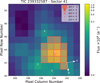 |
Fig. 1 TESS target pixel file for Sector 41 showing GJ 806 as a red circle with a white x, nearby stars as red circles, and the pixels included into the photometry aperture in red. The figure was created with tpfplotter (Aller et al. 2020). |
2.3 Seeing-limited ground photometry
Ground-based seeing-limited observations were taken from a series of observatories in order to determine the rotational period of the host star.
The T150 telescope (Quirrenbach et al. 2022) is a 150 cm Ritchey-Chrètien telescope equipped with a CCD camera Andor Ikon-L DZ936N-BEX2-DD 2k×2k, with a resulting field of view (FOV) of 7.92×7.92 arcmin2. Our set of observations, collected in Johnson V and R filters, consists of 27 epochs obtained during the period October-December 2021. Each epoch typically consisted of 20 exposures of 50 s and 30 s in V and R filters, respectively. All CCD measurements were obtained by the method of fixed aperture photometry using a 1 × 1 binning (no binning). Each CCD frame was corrected in a standard way for bias and flat-fielding. Different aperture sizes were also tested in order to choose the best one for our observations.
GJ806 was monitored in the V-band filter with the 40 cm telescopes of the Las Cumbres Observatory Global Telescope (LCOGT) network (Brown et al. 2013). We obtained 48 epochs between October 8 and December 17, 2021, with the IAC2021B-002 programme (IP: V. Béjar). The instrument mounted on the 40 cm telescopes is a 3k×2k SBIG CCD camera with a pixel scale of 0.571 arcsec providing a FOV of 29.2×19.5 arcmin2. Weather conditions at the observatories were mostly clear during our observations, and the average seeing varied between 1 and 2 arcsecs. Raw data were processed using the BANZAI pipeline (McCully et al. 2018), which includes bad pixel, bias, dark and flat-field corrections for each individual night. Differential aperture photometry of our target with respect to several reference stars were done using AstroImageJ (Collins et al. 2017). We selected the optimal aperture that provides the lower dispersion of the light curves.
GJ806 was also observed from November 2021 to May 2022 with the 0.8 m Joan Oró Telescope (TJO) at the Observatori Astronòmic del Montsec (OAdM), Sant Esteve de la Sarga, Catalonia, using the LAIA 4k×4k CCD camera, which provides a FOV of 30 arcmin with a pixel scale of 0.4 arcsec, and the Johnson R filter. The raw images were reduced with the icat pipeline of the TJO (Colome & Ribas 2006), using dark, bias, and flat-fields images for calibration. We performed differential photometry with AstroImageJ (Collins et al. 2017), using the aperture size that minimized the rms of the resulting relative fluxes, and a selection of the brightest reference stars in the field that did not show variability.
Finally, GJ806 was observed from Entre Encinas y Estrellas4 (e-EYE) in southern Spain. Observations in the B, V, and R filters were taken between October 2021 and May 2022 using a 16″ ODK Corrected-Dall-Kirkham reflector with 16803 CCD chip on an ASA DDM85 mount. The CCD camera is equipped with Astrodon filters. The effective pixel scale is 2.04″ pixel−1 with 3 × 3 binning. Reduction of images and differential aperture photometry of the target and several reference stars were performed using the Lesve photometry package5.
2.4 Spectroscopic observations
2.4.1 CARMENES
The CARMENES6 instrument at the 3.5 m telescope at the Calar Alto Observatory in Almería, Spain, is a dual-channel spectrograph that operates at both the optical (0.52–0.96 µm) and near-infrared (0.96–1.71 µm) wavelengths. The average resolving power for the two wavelength regions is ℛ = 94 600 and ℛ = 80 400, respectively.
GJ 806 was part of the original CARMENES survey of 300 M dwarfs in search of planetary companions, and thus observations started several years prior to the TESS candidate announcement. CARMENES obtained 67 spectra for GJ 806 between 23 April 2016 and 28 October 2021, with a total baseline spanning about 5.5 yr. The exposure times were set to 900s. CARMENES data reduction was performed uniformly using the CARACAL pipeline (Caballero et al. 2016), and radial velocity measurements were extracted using the SERVAL pipeline (Zechmeister et al. 2018). SERVAL RVs were further corrected using measured nightly zero point corrections, as discussed in Trifonov et al. (2020).
The SERVAL pipeline also produces a series of spectral activity indices that can be used to explore the stellar activity signals (see Table D.1). Here we use only the RV data from the CARMENES visible channel. The final CARMENES RV values, along with their uncertainties and BJD time stamp are given in Table D.1. The average signal-to-noise ratio of the observations is 111 at 7370 Å and the average radial velocity precision is 1.5 ms−1.
In addition to the RV monitoring, a single transit of GJ 806b was observed with the CARMENES spectrograph on the night of 30 November 2021. We observed the target simultaneously with the visible and near-infrared channels, collecting a total of 28 high-resolution spectra in each, 10 of them between the first (T1) and fourth (T4) contacts covering the full transit, 8 of them before transit, and 10 after transit. The spectra were taken in good weather conditions with an exposure time of 300 s, ensuring that any planetary absorption line was not spread over more than ~2 pixels during any given exposure, and with a signal-to-noise ratio that varied from 34 to 52 (median value of 44) around 6560 Å and from 73 to 101 (median value of 85) around 10 830 Å.
Fibre A was used to observe GJ 806, while fibre B was placed on the sky in order to monitor the sky emission lines (fibres A and B are permanently separated by 88 arcsec in the east-west direction). The observations were reduced using the CARMENES pipeline caracal, and both fibres were extracted with the flat-optimized extraction algorithm (Zechmeister et al. 2014).
2.4.2 MAROON-X
MAROON-X7 is a stabilized fibre-fed high-resolution (ℛ ≈ 85 000) spectrograph mounted at the 8.1-metre Gemini North telescope on Mauna Kea, Hawaii, USA (Seifahrt et al. 2016, 2018, 2020). MAROON-X has a blue and a red arm, which encompass 500–678 and 654–920 nm, respectively. During an observation the two arms are exposed simultaneously.
We observed GJ 806 with MAROON-X a total of 37 times between 27 October 2021 and 23 November 2021 as part of our ongoing survey of transiting planets identified by TESS around M dwarfs within 30 pc. Exposure times were typically set to 1200 s. When the weather permitted, the target was observed twice a night to allow for precise characterization of the 0.93-day transiting planet.
The data were reduced using a custom package, and radial velocities were extracted using a version of the SERVAL (Zechmeister et al. 2018) pipeline modified for use with MAROON-X data. The red and blue arms were processed separately due to their different wavelength ranges. Thus, the two arms are analysed as independent datasets. The spectra had a peak S/N of around 450 in the red arm and 200 in the blue arm, with accompanying RV precisions of 0.3 ms−1 and 0.4 ms−1, respectively. The higher precision in the red arm is an expected result given the cool host star. As with CARMENES, SERVAL calculated a suite of line indices (Hα, NaD, and CaIRT) and spectral activity indicators (CRX and dLW) to describe the activity of the host star.
2.4.3 HIRES
HIRES obtained 86 spectra for GJ 806 between 2 June 1997 and 26 September 2012, with a total baseline spanning about 15.3 yr. The HIRES RVs were originally published by Butler et al. (2017), and were subsequently reprocessed by Tal-Or et al. (2018), including some nightly zero-point corrections. This last corrected dataset is the one used here (Tal-Or, priv. comm.). The average radial velocity precision is 2.4ms−1.
The complete time series of the radial velocity measurements used in this work, including HIRES, CARMENES, and MAROON-X, is plotted in Fig. 2 and are given in Table D.1.
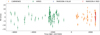 |
Fig. 2 Time series of RV measurements by HIRES, CARMENES VIS, and MAROON-X Red and Blue. |
3 The star
3.1 Stellar parameters
The star GJ 806 was first tabulated in the Bonner Durch-musterung astro-photometric star catalogue (Argelander 1903) with the designation BD+44 3567. However, following the rules of the International Astronomical Union, in this manuscript we use the designation in the first Catalogue of Nearby Stars by Gliese (1969). To avoid confusion with the character string ‘GI’, here we use ‘GJ’ (Gliese & Jahreiß 1988) instead of ‘Gl’ (Gliese) for the acronym.
Because of its relative brightness ( V ~ 10.7 mag) and closeness (d ~ 12 pc), GJ 806 has been frequently investigated on stellar radial velocities (Wilson 1953; Nidever et al. 2002), parallaxes (Strand & Hall 1951; Wagman 1967), magnitudes and colours (Leggett 1992), multiplicity (Fischer & Marcy 1992; Kervella et al. 2019), spectral typing (Kirkpatrick et al. 1991; Rayner et al. 2009), activity (Hawley et al. 1996; Wright et al. 2004), kinematics (Reid et al. 1995; Montes et al. 2001), or characterization in general (Lépine & Shara 2005; Mann et al. 2015; Schweitzer et al. 2019), just to cite a few examples.
GJ 806 was one of the targets of the primary CARMENES guaranteed time observations sample (Reiners et al. 2018), and as such it has been well characterized in the past (e.g. Passegger et al. 2019; Cifuentes et al. 2020). Table 1 summarizes the stellar parameters of GJ 806. We compiled them from Gaia results and preparatory works (Gaia Collaboration 2021; Soubiran et al. 2018) and from CARMENES publications (Fuhrmeister et al. 2020; Marfil et al. 2021; Reiners et al. 2022), or used those that we computed. For simplicity, we refer to Caballero et al. (2022), who exhaustively described each parameter. In the case of log R′HK, we averaged 81 R′HK measurements with Keck/HIRES compiled by Perdelwitz et al. (2021). The age and X-ray emission is discussed in Sect. 4.5, while we derived the rotation period range from photometry, as described below. Additionally, the log R′HK value of −4.92 and the log LCa/Lbol value of −4.92 (Reiners et al. 2022) are consistent with GJ 806 being a very magnetically inactive star.
3.2 Stellar rotation from seeing-limited photometry
GJ 806 has a published rotation period of 19.9 days (Díez Alonso et al. 2019); however, there are clear indications from the TESS light curve, and from the magnetic field value (Reiners et al. 2022) that the rotation period might actually be substantially longer. A quasi-periodic Gaussian process (GP) on the TESS Sector 41 data, masking the transit periods returns a periodicity of  days, significantly longer than the 27-day duration of the TESS sector.
In order to determine GJ 806’s rotational period, we started a photometric follow-up campaign using ground-based telescopes to measure periodic flux variations related to the stellar rotation. We gathered seeing-limited data from the 1.5 m Ritchey-Chrétien telescope at Sierra Nevada Observatory (V and R Johnson filters), the e-EyE telescopes (B and R Johnson filters), the 0.4 m telescopes at Las Cumbres Observatory (V and B Johnson filters), and the 0.8 m Telescopi Joan Oró (TJO) at Observatori Astronomic del Montsec (OAdM; R Johnson filter). Details can be found in Sect. 2.3.
Each photometric dataset was fitted using a linear function to model the mean value and slope of the measurements, and GPs to model the periodic flux variations of the star. The linear function was used to describe long term variations present in the data while the GPs were used to model periodic variations. We used the GP package celerite (Foreman-Mackey et al. 2017), and chose the kernel
![Mathematical equation: $ {k_{ij\,{\rm{Phot}}}} = {B \over {2 + C}}{e^{{{ - \left| {{t_i} - {t_j}} \right|} \mathord{\left/ {\vphantom {{ - \left| {{t_i} - {t_j}} \right|} L}} \right. \kern-\nulldelimiterspace} L}}}\,\left[ {\cos \,\left( {{{2\pi \left| {{t_i} - {t_j}} \right|} \over {{P_{{\rm{rot}}}}}}} \right) + \left( {1 + C} \right)} \right], $](/articles/aa/full_html/2023/10/aa44261-22/aa44261-22-eq2.png) (1)
(1)
where |ti − tj| is the difference between two epochs or observations; B, C, and L are positive constants; and Prot is the stellar rotational period (see Foreman-Mackey et al. 2017 for details). We performed a joint fit of all the photometry available. For each dataset the zero point, we set the slope value of the linear function and the GP kernel constants B, C, L as free parameters. With this approach we can model the different long-term trends seen in the photometry (likely instrumental) and the different sensitivities to the stellar activity of the observed bands. We also note that we allowed the amplitude of the periodic kernel to go to zero for the cases where little to no photometric variations were detected. To constrain the rotation of the star we set the rotational period Prot as a common parameter for all the datasets.
We started the fit with a global optimization of a log posterior function using PyDE8. Then we used the results of the optimization to sample the posterior distribution of the parameters using an Markov chain Monte Carlo (MCMC) procedure with emcee (Foreman-Mackey et al. 2013). The MCMC procedure consisted of 150 chains. We first ran 2000 iterations as a burn-in. The PyDE optimization and this burn-in run were aimed at ensuring convergence. We then ran the MCMC for 10 000 more iterations to properly sample the posterior parameter space. The final parameter values and their respective uncertainties were computed using the percentiles of the posterior distributions: the median values were taken from the 50th percentile and the lower and upper uncertainties were computed using the 16th and 84th percentiles, respectively.
Figure 3 shows all the photometric datasets analysed here and the best-fit model for each time series. Using the procedure described before we find a stellar rotation period of  days. This is in clear disagreement with the value from Díez Alonso et al. (2019). It is noteworthy, however, that a significant peak near 13.6 days appears in the LCO B-band photometric time series, and in the e-EYE R band with sightly shorter periodicity. The period is discussed in the following sections.
Stellar parameters of GJ 806.
3.3 Activityindicators
As mentioned in Sect. 2 the SERVAL analysis of the CARMENES data provides a set of activity indices (see Jeffers et al. 2022 for a full description and discussion of the different indices). Generalized Lomb-Scargle (GLS) periodograms for some of these indices, derived individually for the visible and the near-infrared spectra, are plotted in Fig. 4. Also labelled are some of the periodicities discussed in the data analysis section of this paper that we attribute to planetary signals.
It is clearly seen in Fig. 4 that none of the indices presents significant periodic signals (false alarm probability, FAP < 0.1%) at either the rotation or planetary signals, which are discussed later in this paper. Only the D1 and the Ca II IRT3 indices present a significant periodicity at 39.5 days, which does not have a counterpart in the analysis of the radial velocity values.
To explore these periodicities in more detail, we used the pseudo equivalent width (pEW) of Hα and the two bluer Ca II infrared triplet (IRT) lines as chromospheric indicators, following (Fuhrmeister et al. 2019; see their Table 2 for the used integration bands). Additionally, we used a TiO bandhead index at 7050 Å, defined as the ratio of the integrated flux density in two wavelength bands on both sides of the bandhead. There we followed (Schöfer et al. 2019; see their Table 3 for the wavelength bands used). To each time series of these chromospheric indicators a 3σ clipping was applied to omit outliers due to flaring or weather and instrumental issues. Afterwards we detrended each time series with a polynomial of grade three and then used the GLS periodogram (Zechmeister & Kürster 2009) as implemented in PyAstronomy9 (Czesla et al. 2019) to search for periods in the undetrended and detrended time series. For the 67 usable (of 68 total) spectra of GJ 806 we find a period of 38.629 to 38.996 days in the undetrended data of the four indicators with FAP lower than 0.0036, and a period of 38.690 to 38.934 days in the detrended data with FAP lower than 0.0007. The mean of all eight computed periods (for the four indicators in the undetrended and detrended case) is 38.8 ± 0.2 days (see Fig. B.2).
Finally, to determine the stellar rotation period in a third independent way, we also used the R′HK measurements published by Perdelwitz et al. (2021), which are based on spectra acquired with HIRES (Vogt 1992). The data reduction is also described in Perdelwitz et al. (2021). The 81 values with sufficient signal-to-noise values (S /N > 5 at the Ca II H&K lines) were analysed with a GLS approach (Zechmeister & Kürster 2009) with a period range of 1–1000 days and an oversampling of 1000. The GLS periodogram (see Fig. 5) yields a clear detection at a period of 48.1 d, with a FAP below 10−6.
In summary, using different approaches, we find evidence for GJ 806's rotation period to be at ~34.6, ~38.8, and ~48.1 days. Unfortunately, even considering the large error bars in these period determinations, the results are not compatible. We have to conclude that while the rotation period of GJ 806 is most likely in the range 30–50 days, its true value remains undetermined.
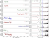 |
Fig. 3 Ground-based photometric observations (left) and generalized Lomb-Scargle (GLS, Zechmeister & Kürster 2009) periodograms (right) for each dataset of GJ 806. Fitting a linear function and a kernel with a periodic term to all the datasets using GPs, we find a stellar rotation period of |

4 Analysis
4.1 Transit photometry
We modelled the transits for the innermost planet (GJ 806 b) using the TESS Sector 15 light curve observed in 30 min cadence, the TESS Sector 41 light curve observed in 2 min cadence, and the MuSCAT2 four-colour light curves from three nights together using PYTRANSIT (Parviainen 2015, 2020; Parviainen & Korth 2020), and show the photometry with the fitted transits models in Fig. 6. The model was parametrized using the mid-transit time at epoch zero, the orbital period, the stellar density, the impact parameter, and the planet-star area ratio (independent of passband or light curve), two quadratic limb darkening coefficients for each passband, an average white noise estimate for each light curve, and a set of linear model covariate coefficients for each light curve10. The limb darkening coefficients were constrained using priors calculated with LDTK (Parviainen & Aigrain 2015), the zero epoch and orbital period had wide normal priors centred around the TESS TOI announcement values11, and the rest of the parameters had uninformative priors obtained after checking that the posterior estimation did not constrain the parameter posteriors. The parameter posteriors agree well with the joint analysis combining photometry and RV information in Sect. 4.3.
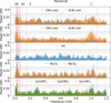 |
Fig. 4 Generalized Lomb-Scargle periodograms of the activity indices derived from SERVAL for the CARMENES data. In all panels, the broken magenta lines indicate the planetary periodicities of 0.96, 6.6, and 13.6 days, and the broken red lines indicate the 19.9-, 34.6-, and 48.1-day possible rotation periods discussed here. In the top two panels, the GLS for the CRX and dLW indices are given independently for the visible and infrared channel spectra. The 10%, 1%, and 0.1% FAP levels are indicated by grey dotted, dash-dotted, and dashed horizontal lines, respectively. |
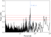 |
Fig. 5 GLS periodogram of R'HK values from the HIRES spectra. The dashed lines in the GLS panel represent the 10%, 1% and 0.1% significance levels. |
4.2 Radial velocities
We searched for planetary signals in the different RV datasets using a GLS approach and computing the theoretical FAP as described in Zechmeister & Kürster (2009). Furthermore, we used juliet12 (Espinoza et al. 2019) to model the detected signals. This Python code is based on other public packages for transit light curves (batman; Kreidberg 2015) and RV (radvel; Fulton et al. 2018) modelling and allows the inclusion of GPs (george, Ambikasaran et al. 2014; celerite, Foreman-Mackey et al. 2017) to model the presence of systematic effects in the data. Instead of using MCMC techniques, juliet uses a nested sampling algorithm to explore all the parameter space and also computes the Bayesian model log-evidence (InZ). This is performed using the MultiNest algorithm (Feroz et al. 2009) via its Python implementation PyMultinest (Buchner et al. 2014). We considered sinusoidal signals with normal priors for the period (P) and uniform priors for the central time of transit (t0) and the semi-amplitude (Kp) to fit the periodicities found in the RVs. We included an instrumental jitter and systemic velocity terms for each of the individual RV datasets.
4.2.1 HIRES RVs
Despite the relatively large number of HIRES measurements, and the long baseline of the dataset, the GLS periodogram does not show significant peaks (FAP ≤ 10%) at periods greater than 1 d. There is a significant peak (FAP ~1%) near 0.92 d, but it is too far away in period to be associated with the signal from the transiting planet GJ 806 b (Fig. 7). We forced a fit to the transiting planet using the parameters from the photometry, but the retrieved model does not recover any significant planet signal. Thus, the HIRES RVs alone do not allow us to characterize the transiting planet, nor do they contain any indication of additional signals.
Although the HIRES data alone cannot find significant planetary signals, two signals at 6.6 and 13.6 days are found when using the other datasets discussed later in this work. If we perform a specific fit for these two signals, with two Keplerians centred around these periods, we find significant detections with semi-amplitudes of  m s−1 and 3.20 + 0.60 m s−1, respectively. Using one Keplerian only for either of the periods or three Keplerians including the transiting planet does not change the results, and the inner transiting planet is not detected (see Table 3).
4.2.2 CARMENES RVs
The GLS of CARMENES RVs presents a very significant peak (FAP ≪0.1%) at ~ 13.6 d and a significant peak (FAP ~ 1%) near 0.92 d (Fig. 7). Because the periodogram region near the transiting planet may be affected by the alias of other signals, we studied the signals in order of significance. We fitted the signal at 13.6 d with a period normal prior (𝒩(l3.608,0.05) [d]). Due to the dispersion in RV, we always used a semi-amplitude uniform prior between 0 and 20 m s−1 (𝒰/(0,20) [m s−1]) for the fitted signals. For the 6.6 d signal, we also used a period normal prior (𝒩(6.64,0.1) [d]). The prior used to fit the transiting planet signal was a period normal prior (𝒩(0.92632,0.001) [d]). After fitting the signal at 13.6 d, the most significant signal of the residuals is at ~6.6 d and the 0.92 d decreases its significance. Thus, we simultaneously fitted the signals at 6.6 d and 13.6 d. The residuals still present a peak near ~ 13 d, but the signal of the transiting planet is clearly detected (FAP ≪ 0.1%). After simultaneously fitting the transiting planet and the 6.6 d and 13.6 d signals, the GLS periodogram of the residuals is mainly flat with only a non-significant peak near 39 d (FAP ~ 10%). This fitting process is illustrated in Fig. 8. Compared with the other models, the three-planet model is preferred for the CARMENES data in terms of Bayesian log-evidence (see Table 2) and minimizes the squared sum of the residuals and the jitter term contribution.
Because the 6.6 d and 13.6 d periods are close to a 1:2 ratio, we explored the hypothesis that one signal is a harmonic of the other. However, in the CARMENES RV analysis, and in the rest of datasets we analyse in the next sections, we found that in general when fitting either of the signals, the other becomes stronger, indicating that we are in fact dealing with either two outer planets in near-resonance or a planet signal and a stellar signal.
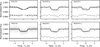 |
Fig. 6 Phase-folded TESS and MuSCAT2 photometry with the median posterior model. The small dots show the original data and the larger dots show data binned to 5 min (TESS) and 10 min (M2) resolution for visualization. The black line shows the posterior median transit model for each passband and dataset. The model for 30 min cadence TESS QLP light curve is supersampled with ten samples per exposure. |
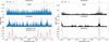 |
Fig. 7 Radial velocity analysis of CARMENES, HIRES, and MAROON-X data. Left: generalized Lomb-Scargle (GLS) periodograms of the HIRES (top), CARMENES (middle), and the two MAROON-X channels (bottom) radial velocity time series. The vertical dotted lines indicate the highest peaks at 13.6 d (magenta), 6.6 d (green), and 0.92 d (orange). The 10%, 1%, and 0.1% FAP levels are indicated by grey dotted, dash-dotted, and dashed lines, respectively. Right: window functions of the HIRES, CARMENES, and MAROON-X channels time series. The vertical dotted lines indicate the 13.6 d (magenta), 6.6 d (green), and 0.92d (orange) periods. |
4.2.3 MAROON-X RVs
The GLS periodograms of the MAROON-X RVs from the red arm, the blue arm, and their combination are similar. They clearly present the transiting planet signal (FAP~ 0.1%) and well-defined peaks at ~6.6d (FAP≪ 0.1%) and ~13.6d (FAP~ 0.1%) (Fig.7). In this section we used the following period priors to fit the 0.9 d, 6.6 d, and 13.6 d signals: 𝒩(0.9263,0.001) [d], 𝒩(6.6,0.1) [d], and 𝒩(13.6,0.1) [d].
In that case, we first fitted the ~6.6 d as it is the strongest signal. In the GLS periodogram of the residuals, the transiting planet then became the biggest peak, followed by the ~ 13.6 d signal, both with FAP ≪0.1%. Then, we simultaneously fitted the 0.92 d and 6.6 d signal. However, after fitting those signals, the 13.6 d signal completely disappeared in the GLS periodogram of the residuals. There is only a long trend that peaks at near ~30d. On the contrary, if we fit the 6.6 d and 13.6 d periods simultaneously, the transiting planet signal disappears in the GLS periodogram of the residuals. When forcing the models to simultaneously fit the 0.92 d, 6.6 d, and 13.6 d signals, the 13.6d signal is not significantly recovered. While we have no clear explanation for these results, it is possible that the 1-day-alias of the 13.6-day signal (at P ≃ 0.931 d) affects the MAROON-X planet signal detections when the transiting planet at 0.92d is fitted. Again our fitting process is illustrated in Fig. 8.
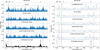 |
Fig. 8 Generalized Lomb-Scargle (GLS) periodograms of CARMENES (left) and MAROON-X (right) RV measurements and the residual RVs after subtraction of different models. In all panels, the 10%, 1%, and 0.1% FAP levels are indicated by grey dotted, dash-dotted, and dashed lines, respectively. Left panels: a) GLS of RV dataset. b) GLS of the RV residuals after fitting the 13.6 d signal (vertical magenta line). c) GLS of the RV residuals after simultaneously fitting the 6.6 d (vertical green line) and 13.6 d signals. d) GLS of the RV residuals after simultaneously fitting the transitting planet (P = 0.926 d, vertical red line), 6.6 d, and 13.6 d signals. Right panels: a) GLS of RV dataset. b) GLS of the RV residuals after fitting the 6.6 d signal (vertical green line). c) GLS of the RV residuals after simultaneously fitting the transiting planet (P = 0.926 d, vertical red line) and 6.6 d signals. d) GLS of the RV residuals after simultaneously fitting the 6.6 d and 13.6 d (vertical magenta line) signals. e) GLS of the RV residuals after simultaneously fitting the transiting planet, 6.6 d, and 13.6 d signals. f) Window function. |
Comparative Bayesian log-evidence.
4.2.4 CARMENES + HIRES RVs
We tried to improve our results by combining the CARMENES and HIRES measurements. The GLS approach combining both RV datasets presents peaks near the transiting planet period with FAP lower than 1%. However, the most significant peak is at 13.6 d and also displays a significant peak at 6.6 d (FAP ~ 0.1%). The GLS is shown in Fig. 9.
Following the same steps as in the CARMENES RV-only analysis, we fitted the 13.6d periodicity with a period normal prior (𝒩(13.6, 0.1) [d]) and, after subtracting this signal, the signal at 6.6 d increased its significance. Thus, we simultaneously fitted a period normal prior (𝒩(6.64, 0.1) [d]) and the 13.6d signal, leading to a refinement of the 6.6d signal properties and constraining the results for the 13.6 d periodicity. When the three periods are simultaneously fitted, using a period normal prior (𝒩(0.9263,0.000032) [d]) for the transiting planet, the RV residuals are mainly flat without significant peaks. Compared with the other models, the three-Keplerian signal model is preferred in terms of Bayesian log-evidence (Table 2), and because it minimizes the squared sum of the residuals and the jitter term contribution.
We also tested the significance of the 0.92d, 6.6d, and 13.6d periods fitting sequentially the three signals, but changing the fitting order. We obtained consistent results in all the cases, enhancing the planetary origin of the signals. Clearly the joint analysis of the combined CARMENES and HIRES data is dominated by the CARMENES signals, and is not significantly different from using CARMENES data alone.
4.2.5 CARMENES + HIRES + MAROON-X RVs
Finally, we analysed the RV measurements from the CARMENES, HIRES, and MAROON-X red and blue arms together. For a quick inspection of the three datasets combined, we used the following period priors to fit the 0.9 d, 6.6 d, and l3.6d signals: 𝒩(0.9263,0.0001) [d], 𝒩(6.64,0.05) [d], and 𝒩(13.60,0.05) [d], respectively. The GLS periodogram of the full combined dataset clearly shows the three signals under study: the transiting planet at 0.93d, and the 6.6d and 13.6d planet candidates. Figure 10 displays the GLS periodograms.
After fitting the three signals under study in the same way as in previous section, the GLS periodogram peaks in the residuals remain under FAP ≤ 10%. The three-Keplerian signal model is still the preferred choice in terms of Bayesian log-evidence (Table 2).
Thus, it would seem that we obtain a consistent picture of the three planetary candidates orbiting GJ 806. A closer inspection of our analysis, however, shows some inconsistencies in the results. The top section in Table 3 summarizes the fitted semi-amplitude (ultimately mass) to each of the three planet candidates. The table shows that the semi-amplitude of the 6.6-day signal is statistically constant no matter what dataset or analysis methods are used. However, the semi-amplitude for the transiting inner planet varies substantially (> 2σ) depending on how many datasets are used, and the third signal at 13.6 days varies its amplitude widely. One would expect a priori that MAROON-X is the best instrument to capture precisely the semi-amplitude of GJ 806b, but the value of the fit to all datasets deviates significantly from the MAROON-X-only fit as a consequence of a possible overestimation of this amplitude in the CARMENES and HIRES data. Moreover, it is possible that the 13.6-day signal, which is detected in the CARMENES and HIRES data, can be of stellar origin, and related to stellar activity (possibly time-varying). Because we were unable to unambiguously determine the rotation period of the host star, as shown in previous sections, this possibility cannot be disregarded.
To account for this possible flaw in our analysis we undertook a series of additional modelling. For a better comparation between datasets and models, and to avoid influences from the used priors, we used the same priors to fit the same signal in all the models showed in Table 3. The priors used in each signal are shown in Table d. Furthermore, the priors for the GP kernels are also shown in Tabled. Those GP prior distributions are the same when the GP is applied to the three different datasets: CARMENES, CARMENES and HIRES individually, and the combined CARMENES+HIRES dataset. In Table 3 we also report the planetary semi-amplitudes reported by a series of models, all including the CARMENES+MAROON-X+HIRES data. The first two models contain simple two- and three-Keplerian signal fits following the same procedures as described in previous sections. In the rest of the models we remove the 13.6-day signal from the CARMENES and/or the HIRES data in different ways, namely: In the reference model, which we name this way as it will be our final adopted model, we removed the 13.6-day signal by fitting a Keplerian signal to the CARMENES+HIRES data and combined the residuals with the MAROON-X data to fit for the 0.9 and 6.6 d signals. In the rest of the models, we fitted the 13.6-day signal using Gaussian processes (GPs). The fit is performed using two different kernels (Quasi-periodic and Exponential Sinus Squared), and applying them to the CARMENES-only data, to the CARMENES and HIRES data individually sharing the GP Prot hyperparameter, and to the combined CARMENES+HIRES dataset. The different combinations give rise to models 2 to 7. The Δ In Z values of each model is also given in Table 3.
Retrieved semi-amplitudes of the three radial velocity signals obtained with each analysis of the different datasets.
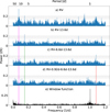 |
Fig. 9 Generalized Lomb-Scargle (GLS) periodograms of the combined CARMENES and HIRES RVs measurements and the residual RVs after subtraction of different models, a) GLS of RV dataset. b) GLS of the RV residuals after fitting the 13.6 d signal (vertical magenta line), c) GLS of the RV residuals after simultaneously fitting the 6.6d (vertical green line) and 13.6 d signals, d) GLS of the RV residuals after simultaneously fitting the transitting planet (P = 0.926 d, vertical red line), 6.6d, and 13.6d signals, e) Window function. The 10%, 1%, and 0.1% FAP levels are indicated by grey dotted, dash-dotted, and dashed lines, respectively. |
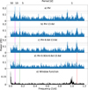 |
Fig. 10 Generalized Lomb-Scargle (GLS) periodograms of CARMENES, HIRES, and MAROON-X red and blue arm RV measurements and the residual RVs after subtraction of different models, a) GLS of RV datasets. b) GLS of the RV residuals after fitting the 13.6 d signal (vertical magenta line), c) GLS of the RV residuals after simultaneously fitting the 6.6 d (vertical green line) and 13.6 d signals, d) GLS of the RV residuals after simultaneously fitting the transiting planet (P = 0.926 d, vertical red line), 6.6 d, and 13.6 d signals, e) Window function. The 10%, 1%, and 0.1% FAP levels are indicated by grey dotted, dash-dotted, and dashed lines, respectively. |
4.2.6 Floating chunk offset analysis
As an independent method of deriving the K-amplitude of the transiting USP planet we applied the floating chunk offset (FCO) method (Hatzes 2014). This method is relatively insensitive to the presence of other long-period signals, and it serves as a check on the K-amplitude found by our previous analyses.
Basically, FCO treats measurements taken on different nights as independent datasets with different zero-point offsets. These nightly datasets are then fit using a fixed period and phase of the transiting planet, but allowing the K-amplitude and nightly zero-point to vary until theχ2 is minimized. FCO acts as a high-pass filter that removes the underlying long-period signals. It also assumes that stellar activity is ‘frozen’ over a single night. In order to apply FCO, two criteria must be met: 1) the periods of other signals must be much longer than that of the short-period transiting planet, and 2) several nights of data are necessary with at least two RV measurements with good time separation.
There were seven nights of CARMENES data with three to four measurements, and only two nights of MAROON-X measurements with good time separation. For the FCO method the number of measurements is relatively sparse, so it is wise to check that the signal of the USP can be detected in the data. To do this we applied an FCO periodogram. The data were fit using a range of trial input periods and allowing the K-amplitude and phase to vary. Figure 11 shows the resulting ;χ2 fit as a function of trial input period. Although there are a large number of ‘alias’ periods present, the best fit is found at the period of the transiting planet.
Applying the FCO method results in an RV amplitude for the USP of Kb = 3.05 ± 0.32 ms−1. However, the presence of additional periods (6.6 d, 13.6 d) found in our previous analyses are short enough that they may introduce a systematic error in the FCO K-amplitude. To check this possibility, we generated a synthetic dataset consisting of the orbit of the USP planet with Kb = 3m s−1 and including the periodic signals (6.6 d and 13.6 d) found by the other analyses. The 13.6-day signal was only added to the synthetic CARMENES dataset. For all input signals the data were sampled using the same time stamps as the observations. No noise was added in this simulation in order to assess a possible offset in the ‘perfect’ case. The simulation resulted in Kb = 3.5 m s−1 implying a systematic offset of +0.5 m s−1 in the FCO value. Applying this correction would result in a final FCO amplitude of Kb = 2.55 ± 0.32 ms−1. However, given that this offset is comparable to the error in the FCO K-amplitude, all that can be said with certainty is that the FCO amplitude recovers the true amplitude within the errors and that the value is entirely consistent with the result derived in Sect. 4.2.5.
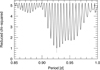 |
Fig. 11 Periodogram of FCO dataset showing reduced χ2 as a function of input period. The vertical dashed line indicates the period of TOI 4481b. |
4.2.7 Best model adoption
As we discuss above, while the CARMENES data alone suggests a three-planet solution, we have reasonable doubts on the nature of the 13.6-day signal. First, MAROON-X data cover nearly two cycles of the 13.6-day signal and the data have enough precision to confidently detect it, but does not retrieve this signal if the transiting planet signal is fitted. We did not find a fully satisfying explanation for this. A first hypothesis was that the 1-day alias of the 13.6-day signal at P = 0.931 d affected the MAROON-X planet signal detection as it is extremely close to the transiting planet period. A second hypothesis is that the 13.6-day signal originates from transient stellar activity in the CARMENES data. Future longer-term RV monitoring observations of the system may solve this issue.
Taking all this in consideration, here we adopted the reference model (2pl ((CARM+HIRES)-13.6 d) + MAROON-X) in Table 3 as our final solution of the RV analysis based on its ∆ ln Z value and its simplicity over the use of GPs. This model’s solution is also consistent with the GJ 806b semi-amplitude solution from MAROON-X data, and has a semi-amplitude for the 13.6-day signal that is close to that from the CARMENES-only data. However we note that, due to the way this model is constructed, it does not fully reflect the degeneracy that might exist in the current dataset between the 13.6 and the 0.92 days signal (due to aliases).
4.3 Joint fit
We simultaneously modelled the TESS and MuSCAT2 photometry and CARMENES, HIRES, and MAROON-X RVs using juliet to obtain the most precise parameters of the GJ 806 planetary system. For the joint fit we adopted the reference model from the RV analysis in Sect. 4.2.5 and only considered transits for planet b. In the process, we took into account the error propagation from the 13.6 d signal subtraction into the CARMENES and HIRES data.
To fit the photometric datasets with juliet, we adopted a linear limb darkening law for the MuSCAT2 photometry and a quadratic limb darkening law for the TESS light curve. The limb darkening coefficients were parametrized with a uniform sampling prior (q1, q2), introduced by Kipping (2013). Additionally, rather than fitting directly the impact parameter of the orbit (b) and the planet-to-star radius ratio (p = Rp/R⋆), we considered the uninformative sample (r1,r2) parametrization introduced in Espinoza (2018). The parameters r1 and r2 ensure a full exploration of the physically plausible values of p and b, with uniform prior sampling. We fixed all the photometric dilution factors to 1 and we added a relative flux offset and a jitter term to the TESS data and for each filter of MuSCAT2.
To save computational time, we narrowed our priors based on the results from the photometry and RV models, but we kept them wide enough to ensure a full exploration of the posterior distribution. The priors used in the joint fit are listed in Table C.2. The median and 68.3% credible intervals of the posterior distributions and the derived planetary parameters are reported in Table 4. Figure C.2 presents the corner plot of the posterior distributions. Figure 12 displays the phase-folded RVs models for the to planets and Fig. C.1 displays the RV time series together with the model. The rms of the residuals is 2.9 ms−1 and the error bar's median error is 2.7 m s−1. We also explored an eccentric solution for planet c; however, this solution is statistically indistinguishable from the circular model (∆ logZ ~ 1), with an eccentricity value that is not well constrained (eccc = 0.07±0.05), and with model parameters consistent within the uncertainties of the values reported in Table 4.
The final analysis result in an inner ultra-short-period planet with a radius of 1.331 ± 0.023 R⊕ and amass of 1.90 ± 0.17 M⊕, and an outer planet with minimum mass of 5.80 ± 0.30 M⊕.
Parameters and 1σ uncertainties for the juliet joint fit model for GJ 806 planetary.
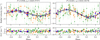 |
Fig. 12 Radial velocities phase-folded to the period and central time of transit (shown above each panel, period units are days and central time of transit t0 units are BJD − 2 457 000) for b (left) and c (right) planets along with the best-fit model (black line) and 3σ confidence intervals (shaded light blue areas). RVs from CARMENES (orange), HIRES (green), and MAROON-X red channel (red) and blue channel (blue) and binned RV (white dots with black error bars) are also shown. The instrument error bars include the extra jitter term added in quadrature. |
Planetary parameters and 1σ uncertainties for the 13.6 d signal.
4.4 The 13.6-day signal as a planet
In our joint fit we determine the planetary nature of GJ 806b and GJ 806c, but we cannot validate the 13.6-day signal as a planet. However, if in the future this signal can be validated, the derived parameters from our reference model in Sect. 4.2.5 are given in Table 5, and the phase-folded CARMENES and HIRES RVs are shown in Fig. 13. The planet would likely be a temperate sub-Neptune, with a minimum mass of 8.50 ± 0.45 M⊕.
4.5 A search for an extended atmosphere
GJ 806b is so far the second ultra-short period planet (P < 1 d) with lower than Earth's mean density discovered around an M dwarf. It joins OI-1685 b in this special category (Bluhm et al. 2021) although GJ 806 is about 2 mag brighter than TOI-1685. As we discuss in the next section, this implies that GJ 806b might posses some type of volatile envelope, either possible remnants of a primordial atmosphere (Howe et al. 2020) or a secondary atmosphere formed through outgassing (Swain et al. 2021). We used a conservative rotational period of the star of 48.1 days to estimate the expected high-energy emission and subsequently the mass loss rate expected in the planet (a shorter rotation period would lead to a larger extreme ultraviolet (XUV) flux estimate). The stellar relation between rotation and X-ray activity by Wright et al. (2011) is used to calculate an X-ray (5–100 Å) luminosity of LX = 2.1 × 1027 ergs−1. The relations in Sanz-Forcada et al. (2011) yield a GJ 806 extreme ultraviolet (XUV, 100–920 Å) luminosity of Leuv = 2.0 × 1028 erg s−1 and a expected mass loss rate in GJ 806 b of 1.5 × 10¹¹ g s−1. This X-ray emission is consistent with an age of ~4 Gyr. Thus, with the aim of detecting a possible extended atmosphere, as described in Sect. 2.4.1, we took transit observations of GJ 806b with CARMENES on 30 November 2021 to measure the Hα and He I planetary absorption.
The transmission spectroscopy data analysis was performed following the same methodology previously employed for CARMENES M dwarf planets in Palle et al. (2020) and Orell-Miquel et al. (2022). The resulting transmission spectrum centred on the spectral regions of the Hα and He I triplet is shown in Fig. 14. The He I triplet transmission spectrum shows a flat spectrum, while the Hα transmission spectrum has an emission-like feature that is a result of stellar variability during the transit. Overall, we found no significant absorption in either of the two line tracers, and we could only place a 3σ upper limit on the excess absorption of 1.5 % and 0.7 % for Hα and He I, respectively.
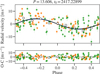 |
Fig. 13 Radial velocities phase-folded to the period and central time of transit (shown above each panel, period units are days and central time of transit t0 units are BJD − 2 457 000) for the 13.6 d signal along with the best-fit model (black line) and 3σ confidence intervals (shaded light blue areas). RVs from CARMENES (orange) and HIRES (green) and binned RVs (white dots with black error bars) are also shown. The instrument error bars include the extra jitter term added in quadrature. |
5 Discussion
5.1 GJ 806b planet properties
As established in previous sections, the GJ8O6 system is composed of an inner ultra-short period planet with a radius of 1.331 + 0.023 R⊕ and a mass of 1.90 + 0.17 M⊕, and at least one outer planet with a 6.6-day period and with minimum mass of 5.80 + 0.30 M⊕. No signs of transits for this outer planet were detected in the TES S light curves (not shown). It is the transiting USP inner planet, however, that makes this system especially interesting.
Figure 15 shows a mass-radius diagram for all know planets with precise mass and radius determinations, where planets around M dwarf stellar types (Teff < 4000 K) are colour-coded. With a mean density of 4.40 ± 0.45 g cm−3 GJ8O6b lies in the pure MgSiO3 model. Thus, GJ8O6b belongs to the growing population of rocky planets in the mass regime of 1–3 M⊕, the majority of which have been discovered orbiting M dwarf stars. GJ8O6b is nearly the same size as two other benchmark targets discovered by CARMENES, GJ 357 b (Luque et al. 2019) and GJ 486 b (Trifonov et al. 2021), although with a much lower density and higher equilibrium temperature.
Focusing on the USP population, as previously mentioned GJ 806b is to date the second ultra-short-period planet (P < 1 d) with a mean density lower than Earth’s discovered around an M dwarf (the third considering the full population of USPs), and the one with the lowest mass (second considering all USPs). Although for the lowest density M dwarf planet, TOI-1685 b, there are some conflicting reports on its final density value (Bluhm et al. 2021; Hirano et al. 2021).
The comparison with planetary models including a light envelope of H/He (Zeng et al. 2019; Fig. 15, left) indicate that such an envelope is very unlikely, well below the 0.1% mass fraction. This is in agreement with our estimation of a very high mass loss rate and the non-detection of an extended atmosphere in Sect. 4.5. It seems that if GJ 806b ever had a primordial H/He atmosphere it was lost a long time ago.
Consistent with this hypothesis is a comparison to synthetic planets computed with the Generation III Bern model of planet formation (Emsenhuber et al. 2021a; Schlecker et al. 2O21 a,b; Mishra et al. 2021). The population of M dwarf planets with 0.5M⊙ host stars presented in Burn et al. (2021) contains ultra-short-period planets (P ≲ 2 d) that are typically of either Earth-like, purely rocky composition or contain ~50% water ice (see Fig. 16), which is supported by the observational population studies of small planets around M dwarfs (Luque & Pallé 2022). Due to atmospheric photoevaporation by their host star, these planets never retain their atmospheres.
GJ 8O6b’s location in the mass-radius diagram strongly suggests that it is a planet devoid of any extended atmosphere. It further occupies a region that is completely unpopulated by synthetic USPs, which may imply that it is a bare core with an intermediate volatile content. If it has accreted all its solids in the form of planetesimals, such an outcome is most likely to occur when the growing planetary core has accreted both inside and outside the water ice line (Burn et al. 2021). This suggests that the planet has migrated inwards significantly during the disc phase, although a giant impact event offers a valid alternative explanation (Emsenhuber et al. 2021b).
Simulations of multi-planet systems with N-body interactions show that a GJ 806-like orbit configuration commonly originates from resonant migration during the disc phase. Once planets lock into a mean-motion resonance, the innermost planet is pushed inside the disc cavity by inward migration of the external planet (Ataiee & Kley 2021; Schlecker et al. 2022). GJ 806 b adds to a small sample of USP planets around mid- and early M dwarfs, contributing to constraints on the scaling of migration traps with stellar host mass.
Turbet et al. (2020) discussed the possibility that planets with a substantial water envelope can develop a supercritical steam atmosphere, which would translate into a slightly larger planetary radius and a slightly lower bulk density than Earth-like planets. Figure 15 (right) indicates that in such a case, GJ8O6b would contain a water mass fraction between 0.1 and 0.01%.
On the other hand, Dorn et al. (2019) discuss how differences in the observed bulk density of small USP planets may occur as a function of radial location and time of planet formation, leading to a class of super-Earths that would have no core and be rich in Ca and Al. This class of planets would have densities 10-20% lower than Earth’s and have very different interior dynamics, outgassing histories, and magnetic fields compared to the majority of super-Earths. This scenario is also compatible with the observed properties of GJ 806b.
With an equilibrium temperature of 940 K, well above the T = 880 K boundary in which rocks start to melt (Mansfield et al. 2019), GJ8O6b is probably a lava world, at least in parts of its surface. Dorn & Lichtenberg (2021) demonstrated how the storage capacity of volatiles in magma oceans has significant implications for the bulk composition. They found that models with and without rock melting and water partitioning lead to deviations in planet radius of up to 16% for fixed bulk compositions and planet mass. While GJ 806b is not a water world, accurate modelling of the mantle melting and volatile redistribution will be needed in order to accurately estimate the bulk water content.
5.2 Atmospheric characterization prospects
We computed the transmission spectroscopy metric (TSM) and emission spectroscopy metric (ESM), as defined by Kempton et al. (2018), to evaluate the prospects for atmospheric characterization of the innermost planet GJ 806 b. Using the stellar and planetary parameters reported in Tables 1 and 4, we obtained  and ESM = 24.1 ± 1.0. Both metric values are well above the respective thresholds of 10 and 7.5 suggested by Kempton et al. (2018) for terrestrial planets, hence classifying GJ 806 b as a high-priority target for transit and eclipse spectroscopic observations. Compared to all confirmed planets with radius Rp < 1.5 R⊕ and given mass measurements from the NASA Exoplanet Archive13, GJ 806 b has the third highest TSM and the highest ESM values (see Fig. 17).
Competing targets for transmission spectroscopy value are L98-59 b (TSM = 51.2; Kostov et al. 2019; Demangeon et al. 2021), LTT 1445 c (TSM = 45.6, Winters et al. 2022), GJ 367 b (TSM = 39.2, Lam et al. 2021), GJ 486 b (TSM = 35.2, Trifonov et al. 2021), and L98-59 c (TSM = 33.9, Demangeon et al. 2021). For emission spectroscopy they are GJ 486 b (ESM = 21.3), GJ 367 b (ESM = 17.2), GJ 1252 b (ESM = 16.5, Shporer et al. 2020), and TOI-431 b (ESM = 15.9, Osborn et al. 2021).
We made use of the online Exoplanet Characterization Toolkit (ExoCTK, Bourque et al. 2021)14 and of the JWST Exposure Time Calculator (ETC)15 to assess the observability of GJ 806 with various spectroscopic modes. The largest spectral coverage can be achieved by combining NIRISS-SOSS (0.6–2.8 μm), NIRSpec-G395H (2.87–5.27 μm), and MIRI-LRS (5–12 μm) instrumental modes. We generated synthetic JWST spectra for a range of atmospheric scenarios using the photo-chemical model ChemKM (Molaverdikhani et al. 2019a,b, 2020), the radiative transfer code petitRADTRANS (Mollière et al. 2019), and ExoTETHyS16 (Morello et al. 2021) to incorporate the instrumental response, including realistic noise and error bars. We considered four models with a H/He gaseous envelope, 1× or 100× solar abundance, without or with haze, and a fifth model with H2O-dominated atmosphere. The models are shown in Fig. 18. The spectroscopic modulations are of several hundred parts per million (ppm) for the cases of H/He-dominated atmospheres, mostly attributable to H2O and CH4 absorption. The spectral features are dampened by a factor of ~2 in the cases with 100× solar metallicity. The presence of haze significantly dampens the spectral features at wavelengths shorter than 2 μm, but some features remain detectable with just one transit observation, even in the presence of enhanced metallicity and haze. Similar trends with enhanced metallicity or haze were also observed in simulations made for other planets (e.g. Espinoza et al. 2022). Interestingly, the spectrum for the H2O-dominated atmosphere presents absorption features of ~60 ppm, that might be detected with high significance by combining a few visits. For reference, we report here our one-visit estimated error bars of 18–22 ppm for the JWST NIRISS-SOSS and NIRSpec-G395H modes with median spectral resolution of R ~ 50, and 42–45 ppm for the MIRI-LRS with wavelength bin sizes of 0.1–0.2 μm.
Owing to the brightness of the host star GJ 806, the near-IR atmospheric features could also be explored with the Hubble Space Telescope (HST) Wide Field Camera 3 (WFC3). In particular, we report one-visit estimated error bars of 21–25 ppm for the HST WFC3-G141 scanning mode (1.075–1.7 µm) using 18 bins, and 27–30 ppm for the WFC3-G102 scanning mode (0.8–1.15 µm) using 12 bins.
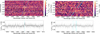 |
Fig. 14 Residuals maps and transmission spectra around the Hα line (left) and He I triplet lines (right). Top panels: residual maps in the stellar rest frame. The planet orbital phase is shown on the vertical axis, the wavelength is on the horizontal axis, and the relative absorption is colour-coded. The dashed white horizontal lines indicate the first and fourth contacts. The cyan lines show the theoretical trace of the planetary signals. Bottom panels: transmission spectra obtained combining all the spectra between the first and fourth contacts. All the wavelengths in this figure are referenced in a vacuum. |
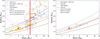 |
Fig. 15 Mass-radius diagrams of all known planets (left) and ultra-short-period planets only (right). Only planets with mass determination better than 30% and radius determination better than 10%, according to the TEPCat database (Southworth 2011), are shown. The orange dots represent the known planets orbiting M dwarfs (Teff < 4000 K) and the grey dots represent those orbiting other stellar types. Overplotted are theoretical models for the planet’s internal composition from Zeng et al. (2019; left) and Turbet et al. (2020; right). GJ 806b is shown as a red dot, while the radius band that GJ 806c occupies is shaded in red. |
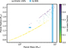 |
Fig. 16 Mass–radius diagram of simulated ultra-short-period planets with periods <2d (from Burn et al. 2021) and GJ 806. Most planets simulated in a core accretion framework (colour-coded by water ice fraction in their cores), are either purely rocky or contain about 50% ice. None of them has an extended atmosphere. GJ 806 b (blue symbol with error bars) is located in the unpopulated space between the two synthetic groups. The radius of GJ 806 c is not constrained (blue stripe). |
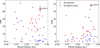 |
Fig. 17 Plot of the TSM and ESM values vs. planetary radius for Earth-sized planets (R < 1.5 R⊙. Red dots correspond to planets orbiting M dwarfs (Teff < 4000 K), while blue dots correspond to all other spectral type hosts. Planet parameters are from the NASA Exoplanet Archive as of 30 March 2022. GJ806b is shown as a red star. |
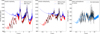 |
Fig. 18 Synthetic JWST transmission atmospheric spectra of GJ 806 b. Left panel: fiducial models with solar abundance and clear atmosphere (solid red line) or haze (solid blue line), and simulated spectral measurements after one transit observation with JWST NIRISS-SOSS, NIRSpec-G395M, and MIRI-LRS configurations. Middle panel: analogous models with metallicity enhanced by a factor of 100. Right panel: fiducial model for a secondary atmosphere made of water, and simulated spectral measurements after combining four transits for each observing mode. |
5.3 Radio emission detection perspectives
The ground-based detection of direct radio emission from Earth-sized exoplanets is not possible as the associated frequency falls below the ≃10 MHz Earth’s ionosphere cutoff. However, in the case of star-planet interaction, the radio emission arises from the magnetosphere of the host star, induced by the exoplanet crossing the star magnetosphere, and the relevant magnetic field is that of the star, B⋆, not the exoplanet magnetic field. Since M-dwarf stars have magnetic fields ranging from about 100 G to above 2–3 kG, their auroral emission falls in the range from a few hundred MHz to a few GHz. This interaction is expected to yield detectable auroral radio emission via the cyclotron emission mechanism (e.g. Turnpenney et al. 2018; Vedantham et al. 2020; Pérez-Torres et al. 2021).
We followed the prescriptions in Appendix B of Pérez-Torres et al. (2021) to estimate the flux density expected to arise from the interaction between the planet GJ 806b and its host star, at a frequency of ~380 MHz, which corresponds to the cyclotron frequency of the star magnetic field of 135 G, taken from Reiners et al. (2022). We show here the radio emission expected to arise from star-planet interaction for a closed dipolar magnetic field geometry, where the interaction between the planet and its host star happens in the sub-Alfvénic regime. Figure 19 shows the predicted flux density as a function of the planet orbital distance, assuming it is not magnetized. The yellow shaded area encompasses the range of values from 0.005 to 0.05 for the efficiency factor, ϵ, in converting Poyinting flux into electron cyclotron maser (ECM) radio emission. The flux density arising from star-planet interaction is expected to be from ~ 160 µJy up to ~25 mJy for the assumed parameters. Thus, radio observations from this system look very promising to probe sub-Alfvénic interaction and, eventually, independently detect radio emission from it. Given the peak frequency, observations at 400 MHz, or even at lower frequencies, would be ideal to probe those scenarios.
6 Conclusions
In this work we presented the discovery of a multi-planetary system around the bright and nearby M1.5 V star GJ 806, using ground-based photometric observations and radial velocity measurements from CARMENES, MAROON-X, and HIRES spectrographs. The star hosts at least two planets. The first is GJ 806b, an ultra-short-period (0.93 d) rocky super-Earth with a radius of 1.331 ± 0.023 R⊕, a mass of 1.90 ± 0.17 Μ⊕, a mean density of 4.40 ± 0.45 g cm−3, and an equilibrium temperature of 940 ± 10 K. The second is GJ 806c, a non-transiting super-Earth with an orbital period of 6.6 d, a mass of 5.80 ± 0.30 Μ⊕, and an equilibrium temperature of 490 ± 5 K. The radial velocity data, the CARMENES data in particular, show evidence of what could be a third super-Earth mass planet (M = 8.50 ± 0.45 Μ⊕) with a period of 13.6 days, but we are unable to unambiguously discard that this signal could be induced by stellar activity, and are thus unable to confirm its planetary nature at this time.
We also estimated the extreme ultraviolet luminosity of GJ 806, and the inferred expected mass loss rate of GJ 806b.
We report the results of a primary transit observation, taken with CARMENES, in search of a possible extended atmosphere focusing on the Hα and He I absorptions lines. We found no significant absorption in either of the two line tracers, but we could set a 3σ upper limit to on the excess absorption of 1.5% and 0.6% for Hα and He I, respectively.
GJ 806b’s relatively low bulk density makes it likely that the planet hosts some type of volatile atmosphere or relatively large water mass fraction, and makes it a very suitable target for atmospheric exploration with JWST and the upcoming ELTs. With a TSM of 43 and an ESM of 24, GJ 806b is the third-ranked terrestrial planet (R < 1.5 R⊕) around an M dwarf suitable for transmission spectroscopy studies using the JWST, and the most promising terrestrial planet for emission spectroscopy studies. We provide simulations of the characterization prospects with the JWST and the HST space telescopes. Additionally, GJ 806b is an excellent target for the detection of radio emission via star-planet interactions.
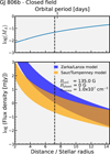 |
Fig. 19 Expected flux density for auroral radio emission arising from star-planet interaction in the system GJ 806 as a function of orbital distance. The interaction is expected to be in the sub-Alfvénic regime (i.e. MA = υrei/υAlfv ≤ 1; top panel) at the location of the planet GJ 806b (vertical dashed line). |
Acknowledgements
CARMENES is an instrument for the Centro Astronómico Hispano-Alemán de Calar Alto (CAHA, Almería, Spain). CARMENES is funded by the German Max-Planck-Gesellschaft (MPG), the Spanish Consejo Superior de Investigaciones Científicas (CSIC), the European Union through FEDER/ERF FICTS-2011-02 funds, and the members of the CARMENES Consortium (Max-Planck-Institut für Astronomie, Instituto de Astrofísica de Andalucía, Landessternwarte Königstuhl, Institut de Ciències de l’Espai, Institut für Astrophysik Göttingen, Universidad Complutense de Madrid, Thüringer Landessternwarte Tautenburg, Instituto de Astrofísica de Canarias, Hamburger Sternwarte, Centro de Astrobiología and Centro Astronómico Hispano-Alemán), with additional contributions by the Spanish Ministry of Economy, the German Science Foundation through the Major Research Instrumentation Programme and DFG Research Unit FOR2544 ‘Blue Planets around Red Stars’, the Klaus Tschira Stiftung, the states of Baden-Württemberg and Niedersachsen, and by the Junta de Andalucía. This paper includes data collected by the TESS mission. Funding for the TESS mission is provided by the NASA Explorer Program. We acknowledge the use of public TOI Release data from pipelines at the TESS Science Office and at the TESS Science Processing Operations Center. Resources supporting this work were provided by the NASA High-End Computing (HEC) Program through the NASA Advanced Supercomputing (NAS) Division at Ames Research Center for the production of the SPOC data products. This research has made use of the Exoplanet Follow-up Observation Program website, which is operated by the California Institute of Technology, under contract with the National Aeronautics and Space Administration under the Exoplanet Exploration Program. The development of the MAROON-X spectrograph was funded by the David and Lucile Packard Foundation, the Heising-Simons Foundation, the Gemini Observatory, and the University of Chicago. The MAROON-X team acknowledges support for this work from the NSF (award number 2108465) and NASA (through the TESS Cycle 4 GI program, grant number 80NSSC22K0117). This work was enabled by observations made from the Gemini North telescope, located within the Maunakea Science Reserve and adjacent to the summit of Maunakea. We are grateful for the privilege of observing the Universe from a place that is unique in both its astronomical quality and its cultural significance. This article is partly based on observations made with the MuSCAT2 instrument, developed by ABC, at Telescopio Carlos Sánchez operated on the island of Tenerife by the IAC in the Spanish Observatorio del Teide. This work makes use of observations from the LCOGT network. Part of the LCOGT telescope time was granted by NOIRLab through the Mid-Scale Innovations Program (MSIP). MSIP is funded by NSF. P.P.P., B.C., D.V. and M.R.M. would like to acknowledge the following iSHELL observers: Claire Geneser, Ahmad Sohani, John Berberian, Patrick Nercessian, Jennah Fayaz, Kevin I Collins and Ian Helm. Based on observations collected at the Observatorio de Sierra Nevada, operated by the Instituto de Astrofisica de Andalucía (IAA-CSIC). This work makes use of observations from the Las Cumbres Observatory global telescope network. The Joan Oró Telescope (TJO) of the Montsec Observatory (OAdM) is owned by the Generalitat de Catalunya and operated by the Institute for Space Studies of Catalonia (IEEC). This material is based upon work supported by the National Science Foundation Graduate Research Fellowship under Grant No. DGE 1746045. We acknowledge financial support from the Agencia Estatal de Investigación of the Ministerio de Ciencia e Innovación and the ERDF ‘A way of making Europe’ through projects PID2021-125627OB-C32 PID2019-109522GB-C5[1:4] PGC2018-098153-B-C3[1,3] ID2019-109522GB-C5[1:4] and the Centre of Excellence ‘Severo Ochoa’ and ‘María de Maeztu’ awards to the Instituto de Astrofísica de Canarias (CEX2019-000920-S), Instituto de Astrofisica de Andalucía (SEV-2017-0709), and Centro de Astrobiología (MDM-2017-0737); the Generalitat de Catalunya/CERCA programme; NASA (Exoplanet Research Program Award #80NSSC20K0251, TESS Cycle 3 Guest Investigator Program Award #80NSSC21K0349, JPL Research and Technology Development, and Keck Observatory Data Analysis); the USA National Science Foundation (Astronomy and Astrophysics Grants #1716202 and 2006517); the Mt. Cuba Astronomical Foundation; R.L. acknowledges funding from University of La Laguna through the Margarita Salas Fellowship from the Spanish Ministry of Universities ref. UNI/551/2021-May 26, and under the EU Next Generation funds. This research was supported by the Excellence Cluster ORIGINS which is funded by the Deutsche Forschungsgemeinschaft (DFG, German Research Foundation) under Germany’s Excellence Strategy – EXC-2094 – 390783311. J.L.-B. acknowledges financial support received from ‘la Caixa’ Foundation (ID 100010434) and from the European Unions Horizon 2020 research and innovation programme under the Marie Slodowska-Curie grant agreement No. 847648, with fellowship code LCF/BQ/PI20/11760023. This research has also been partly funded by the Spanish State Research Agency (AEI) Projects No. PID2019-107061GB-C61 and No. MDM-2017-0737 Unidad de Excelencia ‘María de Maeztu’ – Centro de Astrobiología (INTA-CSIC). This work is partly supported by JSPS KAKENHI Grant Numbers JP17H04574, JP18H05439, Grant-in-Aid for JSPS Fellows, Grant Number JP20J21872, JST CREST Grant Number JPMJCR1761, and the Astrobiology Center of National Institutes of Natural Sciences (NINS; Grant Number AB031010). This article is based on observations made with the MuSCAT2 instrument, developed by ABC, at Telescopio Carlos Sánchez operated on the island of Tenerife by the IAC in the Spanish Observatorio del Teide. M.P.T. acknowledges financial support from the State Agency for Research of the Spanish MCIU through the ‘Center of Excellence Severo Ochoa’ award to the Instituto de Astrofísica de Andalucía (SEV-2017-0709) and through the grant PID2020-117404GB-C21 (MCI/AEI/FEDER, UE). Funding for the TESS mission is provided by NASA’s Science Mission directorate. This paper includes data collected with the TESS mission, obtained from the MAST data archive at the Space Telescope Science Institute (STScI). Funding for the TESS mission is provided by the NASA Explorer Program. STScI is operated by the Association of Universities for Research in Astronomy, Inc., under NASA contract NAS 5–26555. S.V.J. acknowledges the support of the DFG priority programme SPP 1992 Exploring the Diversity of Extrasolar Planets (JE 701/5−1) The results reported herein benefited from collaborations and/or information exchange within the program “Alien Earths” (supported by the National Aeronautics and Space Administration under agreement No. 80NSSC21K0593) for NASA’s Nexus for Exoplanet System Science (NExSS) research coordination network sponsored by NASA’s Science Mission Directorate.
Appendix A Additional stellar parameters
Multi-band photometry of Gl 806a.
Appendix B TESS individual transit light curves
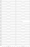 |
Fig. B.1 All individual transits from TESS |
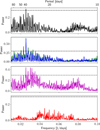 |
Fig. B.2 GLS periodogram of GJ 806 for different detrended time series. The black line (top panel) denotes the GLS of pEW(Hα); the blue and the green line (second panel from top) denote respectively the bluest and the middle line of the Ca II IRT; the violet line (third panel from top) denotes the TiO index; and the red line (bottom panel) denotes the window function. In all panels, the dashed horizontal line marks the FAP of 0.01, above which signals are rated as significant. |
Appendix C Joint fit additional material
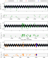 |
Fig. C.1 RV results from the joint fit. CARMENES (orange), HIRES (green), and MAROON-X red channel (red) and blue channel (blue) along with the best-fit model (black line) and the 3σ confidence interval (shaded light blue area). |
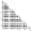 |
Fig. C.2 Corner plot for the orbital parameters fitted with juliet using the joint fit model. The plot makes use of corner.py package (Foreman-Mackey 2016). |
Parameter prior functions used in the juliet joint fit model for GJ 806.
Appendix D RV data
CARMENES radial velocity measurements and spectroscopic activity indicators for GJ 806 from optical spectra.
References
- Aller, A., Lillo-Box, J., Jones, D., Miranda, L. F., & Barceló Forteza, S. 2020, A&A, 635, A128 [NASA ADS] [CrossRef] [EDP Sciences] [Google Scholar]
- Alonso-Floriano, F. J., Morales, J. C., Caballero, J. A., et al. 2015, A&A, 577, A128 [NASA ADS] [CrossRef] [EDP Sciences] [Google Scholar]
- Ambikasaran, S., Foreman-Mackey, D., Greengard, L., Hogg, D. W., & O’Neil, M. 2014 [Google Scholar]
- Argelander, F. W. A. 1903, Eds Marcus and Weber’s Verlag [Google Scholar]
- Ataiee, S., & Kley, W. 2021, A&A, 648, A69 [NASA ADS] [CrossRef] [EDP Sciences] [Google Scholar]
- Bluhm, P., Pallé, E., Molaverdikhani, K., et al. 2021, A&A, 650, A78 [NASA ADS] [CrossRef] [EDP Sciences] [Google Scholar]
- Bourque, M., Espinoza, N., Filippazzo, J., et al. 2021, https://doi.org/18.5281/zenodo.4556863 [Google Scholar]
- Brown, T. M., Baliber, N., Bianco, F. B., et al. 2013, PASP, 125, 1031 [Google Scholar]
- Buchner, J., Georgakakis, A., Nandra, K., et al. 2014, A&A, 564, A125 [NASA ADS] [CrossRef] [EDP Sciences] [Google Scholar]
- Burn, R., Schlecker, M., Mordasini, C., et al. 2021, A&A, 656, A72 [NASA ADS] [CrossRef] [EDP Sciences] [Google Scholar]
- Butler, R. P., Vogt, S. S., Laughlin, G., et al. 2017, AJ, 153, 208 [Google Scholar]
- Caballero, J. A., Guardia, J., López del Fresno, M., et al. 2016, SPIE Conf. Ser., 9910, 99100E [Google Scholar]
- Caballero, J. A., González-Álvarez, E., Brady, M., et al. 2022, A&A, 665, A120 [NASA ADS] [CrossRef] [EDP Sciences] [Google Scholar]
- Caldwell, D. A., Tenenbaum, P., Twicken, J. D., et al. 2020, RNAAS, 4, 201 [NASA ADS] [Google Scholar]
- Cifuentes, C., Caballero, J. A., Cortés-Contreras, M., et al. 2020, A&A, 642, A115 [NASA ADS] [CrossRef] [EDP Sciences] [Google Scholar]
- Collins, K. A., Kielkopf, J. F., Stassun, K. G., & Hessman, F. V. 2017, AJ, 153, 77 [Google Scholar]
- Colome, J., & Ribas, I. 2006, IAU Special Session, 6, 11 [Google Scholar]
- Cutri, R. M., Wright, E. L., Conrow, T., et al. 2021, VizieR Online Data Catalog:II/328 [Google Scholar]
- Czesla, S., Schröter, S., Schneider, C. P., et al. 2019, [record ascl:1906.010] [Google Scholar]
- Demangeon, O. D. S., Zapatero Osorio, M. R., Alibert, Y., et al. 2021, A&A, 653, A41 [NASA ADS] [CrossRef] [EDP Sciences] [Google Scholar]
- Díez Alonso, E., Caballero, J. A., Montes, D., et al. 2019, A&A, 621, A126 [NASA ADS] [CrossRef] [EDP Sciences] [Google Scholar]
- Dorn, C., & Lichtenberg, T. 2021, ApJ, 922, L4 [NASA ADS] [CrossRef] [Google Scholar]
- Dorn, C., Harrison, J. H. D., Bonsor, A., & Hands, T. O. 2019, MNRAS, 484, 712 [Google Scholar]
- Emsenhuber, A., Mordasini, C., Burn, R., et al. 2021a, A&A, 656, A69 [NASA ADS] [CrossRef] [EDP Sciences] [Google Scholar]
- Emsenhuber, A., Mordasini, C., Burn, R., et al. 2021b, A&A, 656, A70 [NASA ADS] [CrossRef] [EDP Sciences] [Google Scholar]
- Espinoza, N. 2018, RNAAS, 2, 209 [Google Scholar]
- Espinoza, N., Kossakowski, D., & Brahm, R. 2019, MNRAS, 490, 2262 [Google Scholar]
- Espinoza, N., Pallé, E., Kemmer, J., et al. 2022, AJ, 163, 133 [NASA ADS] [CrossRef] [Google Scholar]
- Feroz, F., Hobson, M. P., & Bridges, M. 2009, MNRAS, 398, 1601 [NASA ADS] [CrossRef] [Google Scholar]
- Fischer, D. A., & Marcy, G. W. 1992, ApJ, 396, 178 [NASA ADS] [CrossRef] [Google Scholar]
- Foreman-Mackey, D. 2016, J. Open Source Softw., 1, 24 [Google Scholar]
- Foreman-Mackey, D., Hogg, D. W., Lang, D., & Goodman, J. 2013, PASP, 125, 306 [Google Scholar]
- Foreman-Mackey, D., Agol, E., Angus, R., & Ambikasaran, S. 2017, AJ, 154, 220 [NASA ADS] [CrossRef] [Google Scholar]
- Fuhrmeister, B., Czesla, S., Schmitt, J. H. M. M., et al. 2019, A&A, 623, A24 [NASA ADS] [CrossRef] [EDP Sciences] [Google Scholar]
- Fuhrmeister, B., Czesla, S., Hildebrandt, L., et al. 2020, A&A, 640, A52 [NASA ADS] [CrossRef] [EDP Sciences] [Google Scholar]
- Fulton, B. J., Petigura, E. A., Blunt, S., & Sinukoff, E. 2018, PASP, 130, 044504 [Google Scholar]
- Gaia Collaboration (Brown, A. G. A., et al.) 2018, A&A, 616, A1 [NASA ADS] [CrossRef] [EDP Sciences] [Google Scholar]
- Gaia Collaboration (Smart, R. L., et al.) 2021, A&A, 649, A6 [EDP Sciences] [Google Scholar]
- Gliese, W. 1969, Veroeffentlichungen des Astronomischen Rechen-InstitutsHeidelberg, 22, 1 [NASA ADS] [Google Scholar]
- Gliese, W., & Jahreiß, H. 1988, Ap&SS, 142, 49 [NASA ADS] [CrossRef] [Google Scholar]
- González-Álvarez, E., Zapatero Osorio, M. R., Sanz-Forcada, J., et al. 2022, A&A, 658, A138 [NASA ADS] [CrossRef] [EDP Sciences] [Google Scholar]
- Hatzes, A. P. 2014, A&A, 568, A84 [NASA ADS] [CrossRef] [EDP Sciences] [Google Scholar]
- Hawley, S. L., Gizis, J. E., & Reid, I. N. 1996, AJ, 112, 2799 [Google Scholar]
- Hirano, T., Livingston, J. H., Fukui, A., et al. 2021, AJ, 162, 161 [NASA ADS] [CrossRef] [Google Scholar]
- Høg, E., Fabricius, C., Makarov, V. V., et al. 2000, A&A, 355, A27 [NASA ADS] [Google Scholar]
- Howe, A. R., Adams, F. C., & Meyer, M. R. 2020, ApJ, 894, 130 [NASA ADS] [CrossRef] [Google Scholar]
- Jeffers, S. V., Barnes, J. R., Schöfer, P., et al. 2022, A&A, 663, A27 [NASA ADS] [CrossRef] [EDP Sciences] [Google Scholar]
- Jenkins, J. M., Twicken, J. D., McCauliff, S., et al. 2016, in Proc. SPIE, 9913, 99133E [Google Scholar]
- Kemmer, J., Stock, S., Kossakowski, D., et al. 2020, A&A, 642, A236 [EDP Sciences] [Google Scholar]
- Kempton, E. M. R., Bean, J. L., Louie, D. R., et al. 2018, PASP, 130, 114401 [Google Scholar]
- Kervella, P., Arenou, F., Mignard, F., & Thévenin, F. 2019, A&A, 623, A72 [NASA ADS] [CrossRef] [EDP Sciences] [Google Scholar]
- Kipping, D. M. 2013, MNRAS, 435, 2152 [Google Scholar]
- Kirkpatrick, J. D., Henry, T. J., & McCarthy, J. Donald, W., 1991, ApJS, 77, 417 [NASA ADS] [CrossRef] [Google Scholar]
- Königl, A., Giacalone, S., & Matsakos, T. 2017, ApJ, 846, L13 [CrossRef] [Google Scholar]
- Kostov, V. B., Schlieder, J. E., Barclay, T., et al. 2019, AJ, 158, 32 [Google Scholar]
- Kreidberg, L. 2015, PASP, 127, 1161 [Google Scholar]
- Lam, K. W. F., Csizmadia, S., Astudillo-Defru, N., et al. 2021, Science, 374, 1271 [NASA ADS] [CrossRef] [Google Scholar]
- Leggett, S. K. 1992, ApJS, 82, 351 [Google Scholar]
- Lépine, S., & Shara, M. M. 2005, AJ, 129, 1483 [Google Scholar]
- Lindegren, L., Klioner, S. A., Hernández, J., et al. 2021, A&A, 649, A2 [EDP Sciences] [Google Scholar]
- Lopez, E. D. 2017, MNRAS, 472, 245 [NASA ADS] [CrossRef] [Google Scholar]
- Lundkvist, M. S., Kjeldsen, H., Albrecht, S., et al. 2016, Nat. Commun., 7, 11201 [Google Scholar]
- Luque, R., & Pallé, E. 2022, Science, 377, 1211 [NASA ADS] [CrossRef] [Google Scholar]
- Luque, R., Pallé, E., Kossakowski, D., et al. 2019, A&A, 628, A39 [NASA ADS] [CrossRef] [EDP Sciences] [Google Scholar]
- Mann, A. W., Feiden, G. A., Gaidos, E., Boyajian, T., & von Braun, K. 2015, ApJ, 804, 64 [Google Scholar]
- Mansfield, M., Kite, E. S., Hu, R., et al. 2019, ApJ, 886, 141 [Google Scholar]
- Marfil, E., Tabernero, H. M., Montes, D., et al. 2021, A&A, 656, A162 [NASA ADS] [CrossRef] [EDP Sciences] [Google Scholar]
- Mazeh, T., Holczer, T., & Faigler, S. 2016, A&A, 589, A75 [NASA ADS] [CrossRef] [EDP Sciences] [Google Scholar]
- McCully, C., Volgenau, N. H., Harbeck, D.-R., et al. 2018, SPIE Conf. Ser., 10707, 107070K [Google Scholar]
- McDonald, G. D., Kreidberg, L., & Lopez, E. 2019, ApJ, 876, 22 [Google Scholar]
- Mishra, L., Alibert, Y., Leleu, A., et al. 2021, A&A, 656, A74 [NASA ADS] [CrossRef] [EDP Sciences] [Google Scholar]
- Molaverdikhani, K., Henning, T., & Mollière, P. 2019a, ApJ, 883, 194 [Google Scholar]
- Molaverdikhani, K., Henning, T., & Mollière, P. 2019b, ApJ, 873, 32 [NASA ADS] [CrossRef] [Google Scholar]
- Molaverdikhani, K., Henning, T., & Mollière, P. 2020, ApJ, 899, 53 [CrossRef] [Google Scholar]
- Mollière, P., Wardenier, J. P., van Boekel, R., et al. 2019, A&A, 627, A67 [Google Scholar]
- Montes, D., López-Santiago, J., Gálvez, M. C., et al. 2001, MNRAS, 328, 45 [NASA ADS] [CrossRef] [Google Scholar]
- Morello, G., Zingales, T., Martin-Lagarde, M., Gastaud, R., & Lagage, P.-O. 2021, AJ, 161, 174 [NASA ADS] [CrossRef] [Google Scholar]
- Narita, N., Fukui, A., Kusakabe, N., et al. 2019, J. Astron. Telescopes Instrum.Syst., 5, 015001 [NASA ADS] [Google Scholar]
- Nidever, D. L., Marcy, G. W., Butler, R. P., Fischer, D. A., & Vogt, S. S. 2002, ApJS, 141, 503 [Google Scholar]
- Nowak, G., Luque, R., Parviainen, H., et al. 2020, A&A, 642, A173 [NASA ADS] [CrossRef] [EDP Sciences] [Google Scholar]
- Orell-Miquel, J., Murgas, F., Pallé, E., et al. 2022, A&A, 659, A55 [NASA ADS] [CrossRef] [EDP Sciences] [Google Scholar]
- Osborn, A., Armstrong, D. J., Cale, B., et al. 2021, MNRAS, 507, 2782 [NASA ADS] [CrossRef] [Google Scholar]
- Owen, J. E., & Lai, D. 2018, MNRAS, 479, 5012 [Google Scholar]
- Palle, E., Nortmann, L., Casasayas-Barris, N., et al. 2020, A&A, 638, A61 [EDP Sciences] [Google Scholar]
- Parviainen, H. 2015, MNRAS, 450, 3233 [Google Scholar]
- Parviainen, H. 2020, MNRAS, 499, 1633 [NASA ADS] [CrossRef] [Google Scholar]
- Parviainen, H., & Aigrain, S. 2015, MNRAS, 453, 3822 [Google Scholar]
- Parviainen, H., & Korth, J. 2020, MNRAS, 499, 3356 [NASA ADS] [CrossRef] [Google Scholar]
- Parviainen, H., Tingley, B., Deeg, H. J., et al. 2019, A&A, 630, A89 [NASA ADS] [CrossRef] [EDP Sciences] [Google Scholar]
- Passegger, V. M., Schweitzer, A., Shulyak, D., et al. 2019, A&A, 627, A161 [NASA ADS] [CrossRef] [EDP Sciences] [Google Scholar]
- Perdelwitz, V., Mittag, M., Tal-Or, L., et al. 2021, A&A, 652, A116 [NASA ADS] [CrossRef] [EDP Sciences] [Google Scholar]
- Pérez-Torres, M., Gómez, J. F., Ortiz, J. L., et al. 2021, A&A, 645, A77 [NASA ADS] [CrossRef] [EDP Sciences] [Google Scholar]
- Quirrenbach, A., Amado, P. J., Caballero, J. A., et al. 2014, Proc. SPIE, 9147, 91471F [Google Scholar]
- Quirrenbach, A., Passegger, V. M., Trifonov, T., et al. 2022, A&A, 663, A48 [NASA ADS] [CrossRef] [EDP Sciences] [Google Scholar]
- Rayner, J. T., Cushing, M. C., & Vacca, W. D. 2009, ApJS, 185, 289 [Google Scholar]
- Reid, N., Hawley, S. L., & Mateo, M. 1995, MNRAS, 272, 828 [NASA ADS] [Google Scholar]
- Reiners, A., Zechmeister, M., Caballero, J. A., et al. 2018, A&A, 612, A49 [NASA ADS] [CrossRef] [EDP Sciences] [Google Scholar]
- Reiners, A., Shulyak, D., Käpylä, P. J., et al. 2022, A&A, 662, A41 [NASA ADS] [CrossRef] [EDP Sciences] [Google Scholar]
- Ricker, G. R., Winn, J. N., Vanderspek, R., et al. 2015, J. Astron. TelescopesInstrum. Syst., 1, 014003 [Google Scholar]
- Sahu, K. C., Casertano, S., Bond, H. E., et al. 2006, Nature, 443, 534 [Google Scholar]
- Sanchis-Ojeda, R., Rappaport, S., Winn, J. N., et al. 2014, ApJ, 787, 47 [Google Scholar]
- Sanz-Forcada, J., Micela, G., Ribas, I., et al. 2011, A&A, 532, A6 [NASA ADS] [CrossRef] [EDP Sciences] [Google Scholar]
- Schlecker, M., Mordasini, C., Emsenhuber, A., et al. 2021a, A&A, 656, A71 [NASA ADS] [CrossRef] [EDP Sciences] [Google Scholar]
- Schlecker, M., Pham, D., Burn, R., et al. 2021b, A&A, 656, A73 [NASA ADS] [CrossRef] [EDP Sciences] [Google Scholar]
- Schlecker, M., Burn, R., Sabotta, S., et al. 2022, A&A, 664, A180 [NASA ADS] [CrossRef] [EDP Sciences] [Google Scholar]
- Schöfer, P., Jeffers, S. V., Reiners, A., et al. 2019, A&A, 623, A44 [Google Scholar]
- Schweitzer, A., Passegger, V. M., Cifuentes, C., et al. 2019, A&A, 625, A68 [NASA ADS] [CrossRef] [EDP Sciences] [Google Scholar]
- Seifahrt, A., Bean, J. L., Stürmer, J., et al. 2016, SPIE Conf. Ser., 9908, 990818 [NASA ADS] [Google Scholar]
- Seifahrt, A., Stürmer, J., Bean, J. L., & Schwab, C. 2018, SPIE Conf. Ser., 10702, 107026D [NASA ADS] [Google Scholar]
- Seifahrt, A., Bean, J. L., Stürmer, J., et al. 2020, SPIE Conf. Ser., 11447, 114471F [NASA ADS] [Google Scholar]
- Shporer, A., Collins, K. A., Astudillo-Defru, N., et al. 2020, ApJ, 890, L7 [Google Scholar]
- Skrutskie, M. F., Cutri, R. M., Stiening, R., et al. 2006, AJ, 131, 1163 [NASA ADS] [CrossRef] [Google Scholar]
- Smith, J. C., Stumpe, M. C., Van Cleve, J. E., et al. 2012, PASP, 124, 1000 [Google Scholar]
- Snellen, I. A. G., de Kok, R. J., le Poole, R., Brogi, M., & Birkby, J. 2013, ApJ, 764, 182 [Google Scholar]
- Soto, M. G., Anglada-Escudé, G., Dreizler, S., et al. 2021, A&A, 649, A144 [NASA ADS] [CrossRef] [EDP Sciences] [Google Scholar]
- Soubiran, C., Jasniewicz, G., Chemin, L., et al. 2018, A&A, 616, A7 [NASA ADS] [CrossRef] [EDP Sciences] [Google Scholar]
- Southworth, J. 2011, MNRAS, 417, 2166 [Google Scholar]
- Strand, K. A., & Hall, R. G. J. 1951, AJ, 56, 106 [NASA ADS] [CrossRef] [Google Scholar]
- Stumpe, M. C., Smith, J. C., Van Cleve, J. E., et al. 2012, PASP, 124, 985 [Google Scholar]
- Stumpe, M. C., Smith, J. C., Catanzarite, J. H., et al. 2014, PASP, 126, 100 [Google Scholar]
- Swain, M. R., Estrela, R., Roudier, G. M., et al. 2021, AJ, 161, 213 [NASA ADS] [CrossRef] [Google Scholar]
- Szabó, G. M., & Kiss, L. L. 2011, ApJ, 727, L44 [Google Scholar]
- Tal-Or, L., Zechmeister, M., Reiners, A., et al. 2018, A&A, 614, A122 [NASA ADS] [CrossRef] [EDP Sciences] [Google Scholar]
- Trifonov, T., Tal-Or, L., Zechmeister, M., et al. 2020, A&A, 636, A74 [NASA ADS] [CrossRef] [EDP Sciences] [Google Scholar]
- Trifonov, T., Caballero, J. A., Morales, J. C., et al. 2021, Science, 371, 1038 [Google Scholar]
- Turbet, M., Bolmont, E., Ehrenreich, D., et al. 2020, A&A, 638, A41 [NASA ADS] [CrossRef] [EDP Sciences] [Google Scholar]
- Turnpenney, S., Nichols, J. D., Wynn, G. A., & Burleigh, M. R. 2018, ApJ, 854, 72 [Google Scholar]
- Valsecchi, F., Rasio, F. A., & Steffen, J. H. 2014, ApJ, 793, L3 [NASA ADS] [CrossRef] [Google Scholar]
- Vedantham, H. K., Callingham, J. R., Shimwell, T. W., et al. 2020, Nat. Astron., 4, 577 [Google Scholar]
- Vogt, S. S. 1992, in European Southern Observatory Conference and Workshop Proceedings, 40, 223 [NASA ADS] [Google Scholar]
- Vogt, S. S., Allen, S. L., Bigelow, B. C., et al. 1994, SPIE Conf. Ser., 2198, 362 [NASA ADS] [Google Scholar]
- Wagman, N. E. 1967, AJ, 72, 957 [NASA ADS] [CrossRef] [Google Scholar]
- Wilson, R. E. 1953, Carnegie Institute Washington D.C. Publication [Google Scholar]
- Winters, J. G., Cloutier, R., Medina, A. A., et al. 2022, AJ, 163, 168 [NASA ADS] [CrossRef] [Google Scholar]
- Wright, J. T., Marcy, G. W., Butler, R. P., & Vogt, S. S. 2004, ApJS, 152, 261 [Google Scholar]
- Wright, N. J., Drake, J. J., Mamajek, E. E., & Henry, G. W. 2011, ApJ, 743, 48 [Google Scholar]
- Zacharias, N., Finch, C. T., Girard, T. M., et al. 2013, AJ, 145, 44 [Google Scholar]
- Zechmeister, M., & Kürster, M. 2009, A&A, 496, 577 [CrossRef] [EDP Sciences] [Google Scholar]
- Zechmeister, M., Anglada-Escudé, G., & Reiners, A. 2014, A&A, 561, A59 [NASA ADS] [CrossRef] [EDP Sciences] [Google Scholar]
- Zechmeister, M., Reiners, A., Amado, P. J., et al. 2018, A&A, 609, A12 [NASA ADS] [CrossRef] [EDP Sciences] [Google Scholar]
- Zeng, L., Jacobsen, S. B., Sasselov, D. D., et al. 2019, PNAS, 116, 9723 [Google Scholar]
Calar Alto high-Resolution search for M dwarfs with Exoearths with Near-infrared and optical Echelle Spectrographs: http://carmenes.caha.es
M dwarf Advanced Radial velocity Observer Of Neighboring eXo-planets: https://www.gemini.edu/instrumentation/maroon-x
The linear model represents the baseline flux as a weighted sum of auxiliary variables measured simultaneously with the photometry, such as the airmass, x- and y-centroid shifts, and the point spread function (psf) width. The coefficients equal the weights of the auxiliary variables.
All Tables
Retrieved semi-amplitudes of the three radial velocity signals obtained with each analysis of the different datasets.
Parameters and 1σ uncertainties for the juliet joint fit model for GJ 806 planetary.
CARMENES radial velocity measurements and spectroscopic activity indicators for GJ 806 from optical spectra.
All Figures
|
Fig. 1 TESS target pixel file for Sector 41 showing GJ 806 as a red circle with a white x, nearby stars as red circles, and the pixels included into the photometry aperture in red. The figure was created with tpfplotter (Aller et al. 2020). |
| In the text | |
|
Fig. 2 Time series of RV measurements by HIRES, CARMENES VIS, and MAROON-X Red and Blue. |
| In the text | |
|
Fig. 3 Ground-based photometric observations (left) and generalized Lomb-Scargle (GLS, Zechmeister & Kürster 2009) periodograms (right) for each dataset of GJ 806. Fitting a linear function and a kernel with a periodic term to all the datasets using GPs, we find a stellar rotation period of |
| In the text | |
|
Fig. 4 Generalized Lomb-Scargle periodograms of the activity indices derived from SERVAL for the CARMENES data. In all panels, the broken magenta lines indicate the planetary periodicities of 0.96, 6.6, and 13.6 days, and the broken red lines indicate the 19.9-, 34.6-, and 48.1-day possible rotation periods discussed here. In the top two panels, the GLS for the CRX and dLW indices are given independently for the visible and infrared channel spectra. The 10%, 1%, and 0.1% FAP levels are indicated by grey dotted, dash-dotted, and dashed horizontal lines, respectively. |
| In the text | |
|
Fig. 5 GLS periodogram of R'HK values from the HIRES spectra. The dashed lines in the GLS panel represent the 10%, 1% and 0.1% significance levels. |
| In the text | |
|
Fig. 6 Phase-folded TESS and MuSCAT2 photometry with the median posterior model. The small dots show the original data and the larger dots show data binned to 5 min (TESS) and 10 min (M2) resolution for visualization. The black line shows the posterior median transit model for each passband and dataset. The model for 30 min cadence TESS QLP light curve is supersampled with ten samples per exposure. |
| In the text | |
|
Fig. 7 Radial velocity analysis of CARMENES, HIRES, and MAROON-X data. Left: generalized Lomb-Scargle (GLS) periodograms of the HIRES (top), CARMENES (middle), and the two MAROON-X channels (bottom) radial velocity time series. The vertical dotted lines indicate the highest peaks at 13.6 d (magenta), 6.6 d (green), and 0.92 d (orange). The 10%, 1%, and 0.1% FAP levels are indicated by grey dotted, dash-dotted, and dashed lines, respectively. Right: window functions of the HIRES, CARMENES, and MAROON-X channels time series. The vertical dotted lines indicate the 13.6 d (magenta), 6.6 d (green), and 0.92d (orange) periods. |
| In the text | |
|
Fig. 8 Generalized Lomb-Scargle (GLS) periodograms of CARMENES (left) and MAROON-X (right) RV measurements and the residual RVs after subtraction of different models. In all panels, the 10%, 1%, and 0.1% FAP levels are indicated by grey dotted, dash-dotted, and dashed lines, respectively. Left panels: a) GLS of RV dataset. b) GLS of the RV residuals after fitting the 13.6 d signal (vertical magenta line). c) GLS of the RV residuals after simultaneously fitting the 6.6 d (vertical green line) and 13.6 d signals. d) GLS of the RV residuals after simultaneously fitting the transitting planet (P = 0.926 d, vertical red line), 6.6 d, and 13.6 d signals. Right panels: a) GLS of RV dataset. b) GLS of the RV residuals after fitting the 6.6 d signal (vertical green line). c) GLS of the RV residuals after simultaneously fitting the transiting planet (P = 0.926 d, vertical red line) and 6.6 d signals. d) GLS of the RV residuals after simultaneously fitting the 6.6 d and 13.6 d (vertical magenta line) signals. e) GLS of the RV residuals after simultaneously fitting the transiting planet, 6.6 d, and 13.6 d signals. f) Window function. |
| In the text | |
|
Fig. 9 Generalized Lomb-Scargle (GLS) periodograms of the combined CARMENES and HIRES RVs measurements and the residual RVs after subtraction of different models, a) GLS of RV dataset. b) GLS of the RV residuals after fitting the 13.6 d signal (vertical magenta line), c) GLS of the RV residuals after simultaneously fitting the 6.6d (vertical green line) and 13.6 d signals, d) GLS of the RV residuals after simultaneously fitting the transitting planet (P = 0.926 d, vertical red line), 6.6d, and 13.6d signals, e) Window function. The 10%, 1%, and 0.1% FAP levels are indicated by grey dotted, dash-dotted, and dashed lines, respectively. |
| In the text | |
|
Fig. 10 Generalized Lomb-Scargle (GLS) periodograms of CARMENES, HIRES, and MAROON-X red and blue arm RV measurements and the residual RVs after subtraction of different models, a) GLS of RV datasets. b) GLS of the RV residuals after fitting the 13.6 d signal (vertical magenta line), c) GLS of the RV residuals after simultaneously fitting the 6.6 d (vertical green line) and 13.6 d signals, d) GLS of the RV residuals after simultaneously fitting the transiting planet (P = 0.926 d, vertical red line), 6.6 d, and 13.6 d signals, e) Window function. The 10%, 1%, and 0.1% FAP levels are indicated by grey dotted, dash-dotted, and dashed lines, respectively. |
| In the text | |
|
Fig. 11 Periodogram of FCO dataset showing reduced χ2 as a function of input period. The vertical dashed line indicates the period of TOI 4481b. |
| In the text | |
|
Fig. 12 Radial velocities phase-folded to the period and central time of transit (shown above each panel, period units are days and central time of transit t0 units are BJD − 2 457 000) for b (left) and c (right) planets along with the best-fit model (black line) and 3σ confidence intervals (shaded light blue areas). RVs from CARMENES (orange), HIRES (green), and MAROON-X red channel (red) and blue channel (blue) and binned RV (white dots with black error bars) are also shown. The instrument error bars include the extra jitter term added in quadrature. |
| In the text | |
|
Fig. 13 Radial velocities phase-folded to the period and central time of transit (shown above each panel, period units are days and central time of transit t0 units are BJD − 2 457 000) for the 13.6 d signal along with the best-fit model (black line) and 3σ confidence intervals (shaded light blue areas). RVs from CARMENES (orange) and HIRES (green) and binned RVs (white dots with black error bars) are also shown. The instrument error bars include the extra jitter term added in quadrature. |
| In the text | |
|
Fig. 14 Residuals maps and transmission spectra around the Hα line (left) and He I triplet lines (right). Top panels: residual maps in the stellar rest frame. The planet orbital phase is shown on the vertical axis, the wavelength is on the horizontal axis, and the relative absorption is colour-coded. The dashed white horizontal lines indicate the first and fourth contacts. The cyan lines show the theoretical trace of the planetary signals. Bottom panels: transmission spectra obtained combining all the spectra between the first and fourth contacts. All the wavelengths in this figure are referenced in a vacuum. |
| In the text | |
|
Fig. 15 Mass-radius diagrams of all known planets (left) and ultra-short-period planets only (right). Only planets with mass determination better than 30% and radius determination better than 10%, according to the TEPCat database (Southworth 2011), are shown. The orange dots represent the known planets orbiting M dwarfs (Teff < 4000 K) and the grey dots represent those orbiting other stellar types. Overplotted are theoretical models for the planet’s internal composition from Zeng et al. (2019; left) and Turbet et al. (2020; right). GJ 806b is shown as a red dot, while the radius band that GJ 806c occupies is shaded in red. |
| In the text | |
|
Fig. 16 Mass–radius diagram of simulated ultra-short-period planets with periods <2d (from Burn et al. 2021) and GJ 806. Most planets simulated in a core accretion framework (colour-coded by water ice fraction in their cores), are either purely rocky or contain about 50% ice. None of them has an extended atmosphere. GJ 806 b (blue symbol with error bars) is located in the unpopulated space between the two synthetic groups. The radius of GJ 806 c is not constrained (blue stripe). |
| In the text | |
|
Fig. 17 Plot of the TSM and ESM values vs. planetary radius for Earth-sized planets (R < 1.5 R⊙. Red dots correspond to planets orbiting M dwarfs (Teff < 4000 K), while blue dots correspond to all other spectral type hosts. Planet parameters are from the NASA Exoplanet Archive as of 30 March 2022. GJ806b is shown as a red star. |
| In the text | |
|
Fig. 18 Synthetic JWST transmission atmospheric spectra of GJ 806 b. Left panel: fiducial models with solar abundance and clear atmosphere (solid red line) or haze (solid blue line), and simulated spectral measurements after one transit observation with JWST NIRISS-SOSS, NIRSpec-G395M, and MIRI-LRS configurations. Middle panel: analogous models with metallicity enhanced by a factor of 100. Right panel: fiducial model for a secondary atmosphere made of water, and simulated spectral measurements after combining four transits for each observing mode. |
| In the text | |
|
Fig. 19 Expected flux density for auroral radio emission arising from star-planet interaction in the system GJ 806 as a function of orbital distance. The interaction is expected to be in the sub-Alfvénic regime (i.e. MA = υrei/υAlfv ≤ 1; top panel) at the location of the planet GJ 806b (vertical dashed line). |
| In the text | |
|
Fig. B.1 All individual transits from TESS |
| In the text | |
|
Fig. B.2 GLS periodogram of GJ 806 for different detrended time series. The black line (top panel) denotes the GLS of pEW(Hα); the blue and the green line (second panel from top) denote respectively the bluest and the middle line of the Ca II IRT; the violet line (third panel from top) denotes the TiO index; and the red line (bottom panel) denotes the window function. In all panels, the dashed horizontal line marks the FAP of 0.01, above which signals are rated as significant. |
| In the text | |
|
Fig. C.1 RV results from the joint fit. CARMENES (orange), HIRES (green), and MAROON-X red channel (red) and blue channel (blue) along with the best-fit model (black line) and the 3σ confidence interval (shaded light blue area). |
| In the text | |
|
Fig. C.2 Corner plot for the orbital parameters fitted with juliet using the joint fit model. The plot makes use of corner.py package (Foreman-Mackey 2016). |
| In the text | |
Current usage metrics show cumulative count of Article Views (full-text article views including HTML views, PDF and ePub downloads, according to the available data) and Abstracts Views on Vision4Press platform.
Data correspond to usage on the plateform after 2015. The current usage metrics is available 48-96 hours after online publication and is updated daily on week days.
Initial download of the metrics may take a while.