Star-forming content of the giant molecular filaments in the Milky Way

M. Zhang; J. Kainulainen; M. Mattern; M. Fang; Th. Henning

doi:10.1051/0004-6361/201732400

Home

All issues

Volume 622 (February 2019)

A&A, 622 (2019) A52

Full HTML

Free Access

Issue		A&A Volume 622, February 2019


Article Number		A52
Number of page(s)		57
Section		Galactic structure, stellar clusters and populations
DOI		https://doi.org/10.1051/0004-6361/201732400
Published online		04 February 2019

A&A 622, A52 (2019)

Star-forming content of the giant molecular filaments in the Milky Way

M. Zhang (张淼淼)¹^,2, J. Kainulainen³^,1, M. Mattern⁴, M. Fang⁵ and Th. Henning¹

¹ Max-Planck-Institut für Astronomie, Königstuhl 17, 69117 Heidelberg, Germany
e-mail: zhang@mpia.de
² Purple Mountain Observatory, and Key Laboratory for Radio Astronomy, Chinese Academy of Sciences, 210008 Nanjing, PR China
e-mail: miaomiao@pmo.ac.cn
³ Dept. of Space, Earth and Environment, Chalmers University of Technology Onsala Space Observatory, 439 92 Onsala, Sweden
⁴ Max-Planck-Institut für Radioastronomie (MPIfR), Auf dem Hügel 69, 53121 Bonn, Germany
⁵ Department of Astronomy, University of Arizona, 933 North Cherry Avenue, 85721 Tucson, AZ, USA

Received: 1 December 2017
Accepted: 2 November 2018

Abstract

Context. Through observations numerous giant molecular filaments (GMFs) have been discovered in the Milky Way. Their role in the Galactic star formation and Galaxy-scale evolution of dense gas is unknown.

Aims. We investigate systematically the star-forming content of all currently known GMFs. This allows us to estimate the star formation rates (SFRs) of the GMFs and to establish relationships between the SFRs and the GMF properties.

Methods. We identified and classified the young stellar object (YSO) population of each GMF using multiwavelength photometry from near- to far-infrared. We estimated the total SFRs assuming a universal and fully sampled initial mass function and luminosity function.

Results. We uniformly estimate the physical properties of 57 GMFs. The GMFs show correlations between the ¹³CO line width, mass, and size, similar to Larson’s relations. We identify 36 394 infrared excess sources in 57 GMFs and obtain SFRs for 46 GMFs. The median SFR surface density (Σ_SFR) and star formation efficiency (SFE) of GMFs are 0.62 M_⊙ Myr⁻¹ pc⁻² and 1%, similar to the nearby star-forming clouds. The star formation rate per free-fall time of GMFs is between 0.002−0.05 with the median value of 0.02. We also find a strong correlation between SFR and dense gas mass that is defined as gas mass above a visual extinction of 7 mag, which suggests that the SFRs of the GMFs scale similarly with dense gas as those of nearby molecular clouds. We also find a strong correlation between the mean SFR per unit length and dense gas mass per unit length. The origin of this scaling remains unknown, calling for further studies that can link the structure of GMFs to their SF activity and explore the differences between GMFs and other molecular clouds.

Key words: stars: formation / stars: pre-main sequence / ISM: clouds / ISM: structure / infrared: stars

© ESO 2019

1. Introduction

Galactic molecular clouds are known to commonly exhibit filamentary structures (e.g., Barnard et al. 1927; Lynds 1962; Schneider & Elmegreen 1979; Bally et al. 1987; Abergel et al. 1994; Perault et al. 1996; Cambrésy 1999; Hatchell et al. 2005; Myers 2009). Recently, the Herschel results have highlighted the ubiquity of filaments in the interstellar medium (ISM) and their importance in the star formation process (for a recent review, see André et al. 2014). Indeed, studying the impact of filamentary morphology on star formation has become a central topic in current star formation and ISM studies, especially in nearby molecular clouds in which the link between the cloud structure and star formation can be well resolved (e.g., André et al. 2010; Men’shchikov et al. 2010; Schmalzl et al. 2010; Arzoumanian et al. 2011; Hill et al. 2011; Juvela et al. 2012; Hacar et al. 2013; Palmeirim et al. 2013; Alves de Oliveira et al. 2014; Fernández-López et al. 2014; Lee et al. 2014; Storm et al. 2014; Könyves et al. 2015; Roccatagliata et al. 2015; Hacar et al. 2016; Kainulainen et al. 2016; Levshakov et al. 2016; Planck Collaboration Int. XXXII 2016; Planck Collaboration Int. XXXIII 2016; Stutz & Gould 2016; Kainulainen et al. 2017).

Recently, observational studies have discovered and identified a growing number of large-scale filaments with lengths up to ∼100 pc. These objects may be linked to the Galaxy-scale distribution of dense gas and trace features such as the central potential well of spiral arms and spurs sheared off from spiral arms (e.g., Jackson et al. 2010; Kainulainen et al. 2013; Goodman et al. 2014; Ragan et al. 2014; Wang et al. 2015, 2016; Zucker et al. 2015, 2018; Abreu-Vicente et al. 2016; Li et al. 2016). This raises immediately several questions. How relevant are the giant filamentary structures for Galactic star formation? Do they trace Galaxy-scale star formation patterns or trends? Does star formation in them proceed in a similar manner as in other molecular clouds, or does their filamentary nature, or location in the Galaxy, cause a different star formation activity?

Giant filaments have only been identified in the Milky Way since the past few years, and therefore, we still lack a systematic picture of their basic properties and star formation. In general, there is no clear definition for what constitutes “a giant filament”; different studies in literature adopt different definitions. Broadly speaking, a common nominator for these definitions is that the cloud must show clearly elongated shape over some column density regime. For example, the giant filaments can be identified based on the mid-infrared dark features against the Galactic infrared background emission (Ragan et al. 2014; Zucker et al. 2015; Abreu-Vicente et al. 2016) or on the far-infrared or millimeter continuum emission features (Wang et al. 2015; Wang et al. 2016; Li et al. 2016). In the former case the selection leads to clouds whose high column density regions show strong elongation; in the latter case the elongation can be more prominent at lower column densities. The filament candidates identified from column density data are usually considered as continuous clouds only if they show coherence in position-position-velocity space. The velocity coherence can be established with various tracers such as CO (Ragan et al. 2014; Wang et al. 2015; Zucker et al. 2015; Abreu-Vicente et al. 2016), CS and/or NH₃ (Li et al. 2016), and HCO⁺ and/or N₂H⁺ (Wang et al. 2016). As a result of this wide variety of definition techniques, the known giant filaments do not form a uniformly defined sample. Regardless of this ambiguity, it is interesting to consider the basic properties of the objects that fall into this group and compare them with other molecular clouds.

Based on studies exploiting the above methods, the giant filaments have lengths from ∼10 to ∼500 pc (Li et al. 2013) and masses from ∼10³ to ∼10⁵M_⊙. The location of the filaments with respect to the Galactic spiral arms is unclear; efforts have been made to differentiate arm- and inter-arm filaments (Wang et al. 2015, 2016; Zucker et al. 2015, 2018; Li et al. 2016), but the results are sensitive to the uncertainties of the spiral arm models (Vallée 2008, 2017; Reid et al. 2014). Some studies have tried to link the giant filaments to star formation (Henning et al. 2010; Kim et al. 2015; Gong et al. 2016; Xiong et al. 2017). For example, Kim et al. (2015) identified ∼300 young stellar objects (YSOs) in G53.2 that is a filamentary molecular cloud with length of ≳45 pc. Comparison of the YSO population with other nearby star-forming clusters and infrared dark clouds (IRDCs) indicates that G53.2 is similar to the nearby star-forming clusters in age, but at a later evolutionary stage than IRDCs. In contrast, Samal et al. (2015) investigate the star formation activity of a filamentary dark cloud that is part of a ∼20 pc filamentary cloud and found a high protostar fraction (∼70%), which suggests that the filament could still be at a very early evolutionary stage. These studies toward individual long filamentary clouds suggest that giant filaments could exhibit different star formation activities. To estimate the range of SFRs in the giant filaments and to understand the origin of the differing star formation activities, investigation of the star-forming content in a large number of giant filaments is necessary.

In this paper, we present the first systematic investigation of the star-forming content of the Galactic giant molecular filaments (GMFs). We gather together all currently known giant filaments from different studies for a homogeneous analysis. As mentioned before, “giant filament” is a general and not a unique designation, even if the individual studies use well-defined identification criteria. Several different names are used for this type of large-scale filamentary structures, based on the different identification methods, for example, the GMFs (Ragan et al. 2014; Abreu-Vicente et al. 2016), the cold giant filaments (Wang et al. 2015), and the “bones” or “skeleton” of the Galaxy (Goodman et al. 2014; Zucker et al. 2015). We refer to our objects as GMFs for simplicity, reflecting the fact that we estimate their properties mainly based on ¹³CO molecular line data. We identified and classified the YSO population of each GMF using archival multiwavelength photometric catalogs from near- to far-infrared. We further estimated the total star-forming content of the GMFs, based on the assumption of a universal and fully-sampled initial mass function (IMF). This allows us to estimate the star formation rates (SFRs) of the GMFs and correlate the SFRs with the properties of the gas distribution in the GMFs. The resulting relationships between gas and star formation are then compared with literature values and star formation relations. In Sect. 2, we summarize the data used in this paper. In Sect. 3, we describe the methods that are used to obtain the physical properties of the GMFs and to identify YSOs, and we estimate the SFR of each GMF. We investigate the spatial distribution of Class I sources and compare the SFRs of the GMFs with those of nearby star-forming clouds in Sect. 4. In Sect. 5, we compare star formation within GMFs with the canonical star formation relations. We summarize our main conclusions in Sect. 6.

2. Data and point source catalogs

We use the archival multiband photometric catalogs from near-infrared (NIR), mid-infrared (MIR), and far-infrared (FIR) surveys to identify YSO candidates in each Galactic GMF. We also obtain the physical parameters such as mass and column density of each GMF using the ¹³CO molecular line data. Table 1 summarizes these surveys and their purpose and the following sections introduce these data more closely.

Table 1.

Summary of data used in this paper.

2.1. Near-infrared data

We use the archival catalog from the UKIRT infrared deep sky survey (UKIDSS; Lawrence et al. 2007) to obtain near-infrared data for the objects in the northern Galactic plane. For the objects in the southern Galactic plane, there is the archival data from the VISTA variables in the Vía Láctea survey (VVV; Minniti et al. 2010). However, the released catalog of VVV survey is based on aperture photometry, which is clearly unsatisfactory for the crowded fields such as the innermost Galactic center. Thus we downloaded and stacked the archival multiepoch images of VVV survey and then performed point spread function (PSF) photometry. Finally we obtain our own near-infrared photometric catalog for the GMFs in the southern Galactic plane. Due to the saturation problem of UKIDSS and VVV surveys, we also used the 2MASS point source catalog (Skrutskie et al. 2006) for the bright sources.

2.1.1. The UKIDSS/GPS catalog

The UKIDSS Galactic Plane Survey (GPS; Lucas et al. 2008) covers the northern Galactic plane at Galactic latitudes −5 ° < b < 5° in the J, H, K filters with the UKIRT Wide Field Camera (WFCAM; Casali et al. 2007). Compared with 2MASS survey, UKIDSS/GPS is deeper and has better spatial resolution. The median 5σ depths are J = 19.77, H = 19.00, and K = 18.05 mag (Warren et al. 2007). Details about the photometric system, calibration and data processing can be found in Hewett et al. (2006), Hodgkin et al. (2009), Irwin (2008), and Hambly et al. (2008). We use the point source catalog from Date Release 10 Plus (DR10PLUS¹). Because the sources with J < 13.25, H < 12.75, or K < 12.0 mag are affected by saturation (Lucas et al. 2008), we replaced these sources with the photometric results from 2MASS point source catalog (Skrutskie et al. 2006).

2.1.2. PSF photometry for VVV survey

The VVV survey is an ESO public survey, which uses VIRCAM (VISTA InfraRed CAMera; Dalton et al. 2006; Emerson & Sutherland 2010) equipped on the VISTA telecope to observe ∼562 square degrees in the Galactic bulge (−10 ≤ l ≤ 10, −10 ≤ b ≤ 5) and part of the adjacent Galactic plane (−65 ≤ l ≤ −10, −2 ≤ b ≤ 2) in five bands, Z, Y, J, H, K_s, as well as time coverage spanning over five years (Minniti et al. 2010; Saito et al. 2012). The VVV data were processed using VISTA data flow system (VDFS) pipeline at the Cambridge Astronomical Survey Unit (CASU²; Lewis et al. 2010; Saito et al. 2012). The process of VVV data reduction, calibration, and photometry can be found in Saito et al. (2012). Here we should note that the archival photometric catalog from VVV data release is based on aperture photometry which is apparently unsatisfactory for the crowded fields.

We improved an automatic pipeline to perform the PSF photometry on the VVV survey imaging data. This pipeline is based on DAOPHOT algorithm (Stetson 1987) and is written in IDL and Python. We also enabled this pipeline to run in multicore mode, which can significantly decrease the calculating time of PSF fitting. Figure 1 shows the flow chart of the pipeline. For this paper, we have used the data from VSA³ VVV data release 4 (VVVDR4). In order to detect more faint sources, we stacked all multiepoch images for each filter of J, H, and K_s. We mosaiced multi-epoch images chip by chip after excluding the chip images obtained in bad weather condition and then split each stacked chip into the pieces of ∼1000 × 1000 square pixels. The PSF photometry was performed on each piece with PyRAF⁴ which is a command Python scripting language for running IRAF⁵ tasks. Source detection is conducted using DAOFIND task in IRAF with the threshold of S/N > 3. Then we used DAOPHOT PSF task to model the PSF function and ALLSTAR task to obtain the photometric results. The absolute photometric calibration was obtained by a comparison of the instrumental magnitudes of relatively isolated, unsaturated bright sources with the counterparts in the VVV archival CASU catalog. The 2MASS filters are also slightly different from the VISTA filters. To obtain the photometric results in 2MASS photometric system, we calculated the transformations from VISTA to 2MASS system tile by tile using the method suggested by Soto et al. (2013). The saturated sources in our final catalog are also replaced by 2MASS magnitudes.

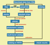Fig. 1.

Flow chart of our automatic PSF-fitting pipeline that is used to do the PSF photometry on the VVV survey imaging data.

Figure 2 shows the K_s magnitude distribution of the sources detected by PSF photometry (black line) and sources in VVV archival CASU catalog (red line) in two tile regions, of which “b332” is a tile in Galactic bulge while “d095” is a tile in Galactic disk. Our PSF photometry can reach ∼1−2 mag deeper than aperture photometry in the K_s band.

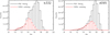Fig. 2.

K_s magnitude distributions of the sources detected by PSF photometry (black line) and sources in VVV CASU catalog (red line) for tile “b332” (left panel) and tile “d095” (right panel).

2.2. Mid-infrared data

We used the archival catalogs from the Spitzer galactic plane surveys, GLIMPSE (Benjamin et al. 2003; Churchwell et al. 2009) and MIPSGAL (Carey et al. 2009), to trace the mid-infrared emission of the point sources. In this paper, we have used the merged GLIMPSE catalog released by Spitzer Science Center (2009) and the high quality 24 μm point source catalog released by Gutermuth & Heyer (2015). We also use the bright sources from the AllWISE (Wright et al. 2010) catalog as a supplement due to the saturation problem of Spitzer surveys. However, some bright source such as the massive young stellar objects (MYSOs) are still saturated on the WISE images. To include the MYSOs in our final catalog, we used the massive protostar catalog from the Red MSX Source (RMS) survey (Lumsden et al. 2013).

2.3. Far-infrared Herschel Hi-GAL catalog

The Herschel Infrared Galactic plane survey (Hi-GAL; Molinari et al. 2010) is a Herschel key project that initially aimed at observing the inner Galactic plane of |l|< 60°, |b|< 1° and was subsequently extended to the entire Galactic plane (Elia et al. 2013). Hi-Gal uses the Photodetector Array Camera and Spectrometer (PACS; Poglitsch et al. 2010) and the Spectral and Photometric Imaging REceiver (SPIRE; Griffin et al. 2010) in parallel mode (pMode) to sample the spectral energy distribution (SED) at 70, 160, 250, 350, and 500 μm simultaneously with the spatial resolution of ∼6″, 12″, 18″, 24″, and 35″, respectively. Details of the Hi-GAL observing strategy, data reduction, calibration, source detection and photometry can be found in Molinari et al. (2010, 2016), and Traficante et al. (2011). In this paper, we use the compact source catalog from Hi-GAL DR1 which is the first public data release and limited to the inner Galactic plane (−70 ° ≤l ≤ 68°, |b|≤1°; Molinari et al. 2016).

2.4. Multiband photometric catalog

We use STILTS (Taylor 2006) to merge the catalogs in different wavelength bands. Molinari et al. (2016) presented five single band catalogs at 70, 160, 250, 350, and 500 μm. First we crossmatched these catalogs to obtain a merged Hi-GAL catalog. Dunham et al. (2008) suggested 70 μm as a crucial wavelength for the embedded protostars and found a tight correlation between the protostellar luminosity and the flux at 70 μm. Thus the detection at 70 μm of the compact sources has been used to distinguish protostars from starless cores (Bontemps et al. 2010; Könyves et al. 2010, 2015; Giannini et al. 2012; Elia et al. 2013; Rygl et al. 2013; Gaczkowski et al. 2013). The objective of this paper is to identify young stellar objects (YSOs). Thus here we only care about the compact sources with 70 μm detections in the Hi-GAL photometric catalogs. Therefore, we used the 70 μm compact source catalog as the reference catalog. Any other Hi-GAL catalog is matched with the reference catalog with the tolerances of 12″, 18″, 24″, and 35″, corresponding to the spatial resolutions at 160, 250, 350, and 500 μm, individually. The merged Hi-GAL catalog only includes the compact sources with 70 μm detections. Secondly, we matched the MIPSGAL catalog with the GLIMPSE catalog using a tolerance of 2″ to obtain an merged Spitzer catalog and then matched the merged Hi-GAL catalog with this merged Spitzer catalog using a tolerance of 6″. To add the near-infrared catalog, we checked the counts of matched sources between the near-infrared catalog and the Spitzer+Herschel catalog using different tolerances and finally selected a tolerance of 0.6″ to match the near-infrared catalog with the merged Spitzer+Herschel catalog. This multiband photometric catalog will be used for the subsequent YSO identification.

2.5. Molecular line data

We used ¹³CO (J = 1 − 0) data cubes from the GRS (Jackson et al. 2006) and ThrUMMS (Barnes et al. 2015) surveys to estimate the physical parameters of the GMFs such as the column density, mass, and velocity dispersion.

2.5.1. GRS data

The Boston University-FCRAO Galactic Ring Survey (GRS; Jackson et al. 2006) use the Five College Radio Astronomy Observatory (FCRAO) 14 m telescope to survey the partial Galactic plane of 18 ° < l < 55.°7, |b|≲1° and 14 ° < l < 18°, |b|≲0.5° at the ¹³CO (J = 1 − 0) frequency (ν₀ = 110.2 GHz) with a beam size of 46″. The velocity resolution of GRS is about 0.2 km s⁻¹ and the RMS noise is about 0.27 K per 0.2 km s⁻¹. The main beam efficiency of the antenna is 0.48. The GRS data are available online⁶. We used the FITS data cubes of GRS data release.

2.5.2. ThrUMMS data

The Three-mm Ultimate Mopra Milky Way Survey (ThrUMMS; Barnes et al. 2015) use 22 m Mopra telescope to survey the fourth Galactic quadrant of 300 ° < l < 360°, |b|≲1° in the J = 1 − 0 lines of ¹²CO, ¹³CO, C¹⁸O, and CN with a spatial resolution of 72″ and a velocity resolution of ∼0.3 km s⁻¹. The sensitivities for ¹³CO are about 0.7 K channel⁻¹. The ThrUMMS data is also available online⁷. We used the data release 4 (DR4) FITS cubes for ¹³CO.

3. Methods

In this section we describe the sample selection of the GMFs and the determination of their physical parameters (Sect. 3.1), YSO identification and classification (Sect. 3.2) and estimation of star formation rate in each GMF (Sect. 3.3).

3.1. GMF sample

We constructed our sample by combining the samples of giant filaments identified by Ragan et al. (2014), Wang et al. (2015, 2016), Zucker et al. (2015), Abreu-Vicente et al. (2016), and Li et al. (2016), including 121 Galactic giant filaments with the length of > 10 pc. Table 2 summarize the sample information. We note that Li et al. (2016) presented a large filament sample based on the data from APEX Telescope Large Area Survey of the Galaxy (ATLASGAL; Schuller et al. 2009). We have only included the velocity coherent filaments with lengths of >10 pc of their sample.

Table 2.

Summary of giant filaments identified with different dataset and criteria.

Our agglomerate sample of 121 giant filaments has been identified using different methods and different datasets. Thus their physical parameters such as mass are also calculated based on different gas tracers and methods. To obtain a systematic investigation of the filament properties, we re-estimated their parameters using a uniform method.

Of 121 giant filaments, 82 are covered by the GRS or ThrUMMS survey data. We also excluded three filaments that show self-absorption, four filaments that are not fully covered by ¹³CO data, and 18 redundant filaments that are identified several times by different papers. We integrated the ¹³CO data cubes over the velocity range of each filament to obtain maps of integrated intensity. Assuming a uniform excitation temperature of 10 K and ¹³CO abundance of [¹³CO/H₂] ∼ 1.2 × 10⁻⁶ (Frerking et al. 1982; Wilson & Rood 1994), we obtain ¹³CO-based column density maps for 56 giant filaments. The uncertainties of these column density maps are mainly from the variation of excitation temperature and ¹³CO abundance. We note that we use the extinction map constructed with the technique of Kainulainen & Tan (2013) for the “Nessie” filament (Mattern et al. 2018). The details about how to obtain the column density maps and associated uncertainties can be found in Appendices A and D.

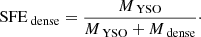
We used the extinction contour level of A_V = 3 mag to define the boundaries of the GMFs. We note as a caveat for the later comparisons that this value is slightly higher than the values used by Lada et al. (2010) (A_V ∼ 1 mag) and Heiderman et al. (2010), Evans et al. (2014) (A_V = 2 mag). We also checked each GMF and made sure that its boundary can morphologically separate the filament from the surrounding diffuse gas. As examples, Figs. 3–9 (left panels) show the column density maps of seven GMFs; the column density maps of the other GMFs can be found in Figs. G.1–G.49.

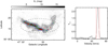Fig. 3.

Overview of GMF 39 (CFG047.06+0.26). Left panel: background is CO-based extinction map. The black and blue contours represent the visual extinction of A_V = 3 and 7 mag, individually. The dashed ellipses are obtained through fitting the pixels inside the regions with A_V > 3 mag. The identified YSOs are labeled with red filled circles (Class I) and green pluses (Class II). Right panel: ¹³CO average spectrum for the region with A_V > 3 mag. The red vertical lines mark the GMF velocity range.

Fig. 4.

Overview of GMF 43 (GMF54.0−52.0). Others are same as Fig. 3.

Fig. 5.

Overview of GMF 44 (GMF307.2−305.4). Others are same as Fig. 3.

Fig. 6.

Overview of GMF 45 (GMF309.5−308.7). Others are same as Fig. 3.

Fig. 7.

Overview of GMF 46 (GMF319.0−318.7). Others are same as Fig. 3.

Fig. 8.

Overview of GMF 52 (GMF335.6−333.6a). Others are same as Fig. 3.

Fig. 9.

Overview of GMF 54 (GMF341.9−337.1). Others are same as Fig. 3.

For the Nessie, the high resolution extinction map has projection effects due to the lack of information along the line-of-sight although the Nessie has been confirmed as a velocity coherent filament (Jackson et al. 2010). To crop the extinction map to the Nessie, we introduced a polygon around the cloud. The area selection is mainly based on by eye inspection of the derived column density map with orientation on the A_V = 3 mag contour and the observations published by Jackson et al. (2010; Mattern et al. 2018).

We obtain the dense gas mass by integrating the ¹³CO-based extinction map above A_V = 7 mag in each GMF. We note that the definitions of dense gas vary in literature. Evans et al. (2014) adopt the extinction contour of A_V = 8 mag to calculate the M_dense. Ragan et al. (2014) and Abreu-Vicente et al. (2016) use the continuum millimeter observations such as ATLASGAL to trace the dense gas. The threshold that they adopted based on the sensitivity of ATLASGAL corresponds to A_V ∼ 10 mag. Our choice is motivated by the choice of Lada et al. (2010). They use the extinction contour of A_K = 0.8 mag to measure the M_dense, corresponding to A_V ≈ 7 mag if using the extinction law suggested by Xue et al. (2016).

Based on the column density map and the defined boundary of each object, we estimated the basic physical parameters of the 57 GMFs (see Appendix B for details). Table H.1 lists these parameters. We note that the uncertainties listed in Table H.1 do not include the distance uncertainty.

3.2. YSO identification and classification

3.2.1. YSO identification

YSOs usually show excessive infrared emission that can be used to distinguish them from field stars. Based on the slope of SEDs, Lada & Wilking (1984) and Lada (1987) developed a “standard” empirical classification scheme to indicate the different evolutionary stages of YSOs. Some authors use the infrared spectral index to identify YSO candidates in the star-forming regions (Mallick et al. 2013; Kim et al. 2015). YSOs can be also identified by the multicolor criteria (i.e., color–color and color-magnitude diagrams). In the present work, we have combined several methods that are based on the infrared multicolor criteria to identify YSO candidates (Gutermuth et al. 2008, 2009; Robitaille et al. 2008; Veneziani et al. 2013; Koenig & Leisawitz 2014; Saral et al. 2015). This method uses the SEDs of sources from 1 to 500 μm and can efficiently mitigate the effects of contamination. The details about this method can be found in the Appendix C. In general, we searched through several tens of millions sources and selected 36394 sources with the infrared excess in 57 GMFs, of which 4821 (∼13%) are AGB candidates. The 31573 YSO candidates include 5611 Class I candidates, 22609 Class II candidates, 384 transition disk candidates, 2874 prostellar objects, and 95 massive YSO candidates (see Appendix C for the criteria of different classifications).

We note that the identification of the bona-fide YSOs needs the spectroscopic observations, which are not available here. However, in the subsequent context we will simply use “YSOs” and “Class I/II sources” to refer “YSO candidates” and “Class I/II candidates” for convenience although they are just candidates.

3.2.2. Correcting for extinction

Considering that our objects are located at large distances and associated with dense gas, it is necessary to correct the flux densities of the YSOs for extinction. We note that we only wish to correct for the diffuse foreground extinction rather than the local extinction from dense cores surrounding protostars (Evans et al. 2009; Dunham et al. 2015). We use the method suggested by Fang et al. (2013) and Zhang et al. (2015) to deredden the photometry of YSOs.

Firstly, for the sources with J, H, K_s detections, the extinction is obtained by employing the JHK_s color–color diagram. A detailed description can be found in Fang et al. (2013) and Zhang et al. (2015). Here we only summarize a few aspects of this scheme. The location of each YSO in the JHK_s color–color diagram depends on both its intrinsic colors and its extinction. Figure 10 shows the J − H versus H − K_s color–color diagram of the YSOs in the GMF 39 (CFG047.06+0.26). Given the different origins of intrinsic colors of YSOs, the color–color diagram is divided into three subregions. In region 1, the intrinsic color of [J − H]₀ is simply assumed to be 0.6; in region 2, the intrinsic color of a YSO is obtained from the intersection between the reddening vector and the locus of main sequence stars (Bessell & Brett 1988); in region 3, the intrinsic color is derived from where the reddening vector and the classical T Tauri star (CTTS) locus (Meyer et al. 1997) intersects. Then the extinction values of YSOs are estimated from observed and intrinsic colors with the extinction law of Xue et al. (2016). Secondly, for other sources (outside these three regions or without detections in JHK_s bands), their extinction is estimated with the median extinction values of surrounding Class II sources and transition disks that have extinction measurements in the first step.

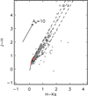Fig. 10.

H − K_s versus J − H color–color diagram for the YSOs in the GMF 39 (CFG047.06+0.26). The solid curves show the intrinsic colors for the main-sequence stars (black) and giants (red; Bessell & Brett 1988), and the dash-dotted line is the locus of T Tauri stars from Meyer et al. (1997). The dashed lines show the reddening direction, and the arrow shows the reddening vector. The extinction law we adopted is from Xue et al. (2016). We note that the dashed lines separate the diagram into three regions marked with numbers 1, 2, and 3 in the figure. We use different methods to estimate the extinction of YSOs in different regions (see the text for details).

With extinctions obtained using above method, we deredden the SED of each YSO using the extinction law of Xue et al. (2016).

3.2.3. YSO classification

We reclassify the identified YSOs after the extinction correction using the dereddened SEDs of the YSOs. There are two main YSO classification schemes, one is based on the spectral index (α, Greene et al. 1994) and the other employs the bolometric temperature (T_bol, Chen et al. 1995). There are both advantages and disadvantages for these two classification schemes.

The source’s spectral index, in other words, the slope of the source’s SED defined as

$\begin{matrix} α = \frac{d log (λ S_{λ})}{d log (λ)}, \end{matrix}$ $\begin{aligned} \alpha = \frac{d\,{\text{ log}}(\lambda S_{\lambda })}{d\,{\text{ log}}(\lambda )}, \end{aligned}$ (1)

where S_λ is the flux density at wavelength λ, can be used to classify the evolutionary state of the source. By fitting the dereddened SEDs from 2 to 24 μm, the YSOs can be classified as Class I, “Flat spectrum”, Class II, and Class III sources based on the scheme suggested by Greene et al. (1994).

The bolometric temperature of a source that is defined as (Myers & Ladd 1993).

$\begin{matrix} T_{bol} = 1.25 \times 10^{- 11} \frac{\int_{0}^{\infty} ν S_{ν} d ν}{\int_{0}^{\infty} S_{ν} d ν} K, \end{matrix}$ $\begin{aligned} T_{\mathrm{bol}} = 1.25 \times 10^{-11} \frac{\int _{0}^{\infty } \nu {S_{\nu }}{\mathrm{d}}\nu }{\int _{0}^{\infty } S_{\nu }{\mathrm{d}}\nu }\,{\mathrm{K}}, \end{aligned}$ (2)

where S_ν is the source’s flux density at frequency ν, can be also used to determine the evolutionary stage of a source. In practice, we calculate these integrals using the trapezoid rule to integrate over the finitely sampled SEDs following the suggestion of Dunham et al. (2008, 2015). Based on their bolometric temperature, YSOs can be classified as Class 0, Class I, and Class II sources according to the classification scheme of Chen et al. (1995).

Figure 11 shows the dereddened α_{2 − 24μm} that is calculated based on the SED from 2 to 24 μm and T_bol of YSOs in the sample of GMF 39 (CFG047.06+0.26). The dashed lines indicate the classification criteria.

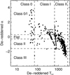Fig. 11.

Dereddened α and T_bol of YSOs in the GMF 39 (CFG047.06+0.26). The dashed lines show the boundaries of YSO classification schemes (Greene et al. 1994; Chen et al. 1995).

The spectral index of α_{2 − 24μm} has been widely used for YSO classification. However, α_{2 − 24μm} is not sensitive for the protostars that are identified based on the emission at 70 μm: some of these protostars only have weak emission or are even invisible at 2−24 μm.

The bolometric temperature T_bol is more appropriate for the embedded objects and can be used to isolate Class 0 sources (Evans et al. 2009). However, Dunham et al. (2015) found that the measured T_bol of YSOs with disks is mostly determined by the spectral type of the central source and the value of T_bol is correlated with the range of SED that is used to calculate T_bol (see Appendix C of Dunham et al. 2015 for details), which means that the T_bol measured with different ranges of SEDs of YSOs with the similar spectral types would be clustered into different narrow T_bol ranges. This effect can be also used to explain the patterns in Fig. 11. As Dunham et al. (2015) pointed, T_bol is not a good discriminator between Class II and Class III.

Taking into account the issues described above, we decided to combine α_{2 − 24μm} and T_bol to classify the YSOs:

The protostellar objects that are identified based on the emission at 70 μm are classified as Class I sources.
The YSOs that have α_{2 − 24μm} measurements are classified as Class I (α_{2 − 24μm} ≥ 0.3) and Flat (−0.3 ≤ α_{2 − 24μm} < 0.3) sources. The YSOs without α_{2 − 24μm} measurements but with T_bol ≤ 650 K are also classified as Class I sources.
Excluding the Class I and Flat sources classified in step 1 and 2, the remaining YSOs are classified as Class II sources if they a) have α_{2 − 24μm} measurements and −1.6 ≤ α_{2 − 24μm} < −0.3 or b) have not α_{2 − 24μm} measurements but 650 < T_bol ≤ 2800 K.
The remaining YSOs are classified as Class III sources.

Finally, each of YSOs can be classified as Class I, Flat, Class II, or Class III source.

The status of Flat sources is not very clear and they are generally considered to be a transitional class. Heiderman & Evans (2015) presented an HCO⁺ survey of Class 0+I and Flat YSOs in the Gould Belt clouds and they defined a Class 0+I+Flat source that is associated with HCO⁺ emission as a stage 0+I source which consists of a star and disk embedded in a dense, infalling envelope (i.e., a bona fide protostar). Heiderman & Evans (2015) found that ∼50% of Flat sources are associated with HCO⁺ emission. They also found that the fraction of sources that are associated with HCO⁺ emission is ≳70% for the sources with bolometric luminosity (L_bol) of ≳1 L_⊙, which means that the bright Flat sources have high probability to be bona fide protostars.

Considering the distances of our GMFs (>2 kpc), we can only detect the bright Flat sources that have high probability to be the bona fide protostars. Therefore, in this paper we simply group together the Flat sources as Class I sources and refer to them together as “Class I sources”.

3.2.4. Estimating and excluding contamination

Considering the distances of the GMFs (>2 kpc), our YSOs are contaminated by foreground sources such as the foreground AGBs and the foreground YSOs which are associated with the molecular clouds that are located between us and the GMFs. In Sect. 3.2.1, we have isolated a bunch of AGBs using the multicolor criteria (see Appendix C). However, because AGB stars can mimic the colors of YSOs, it is difficult to exclude AGBs only based on the color criteria. Simply assuming an universal spatial distribution for the Galactic AGB stars (Jackson et al. 2002; Robitaille et al. 2008), the contamination fraction of foreground AGBs mainly depends on the distances of the GMFs. On the other hand, the contamination fraction of foreground YSOs mainly depends on the number of molecular clouds that are located before the GMFs, which is related with the distances and the Galactic longitudes and latitudes of the GMFs.

We used the A_V values obtained in Sect. 3.2.2 and the 3D extinction map to isolate the foreground contamination. By comparing the 2MASS photometry to the stellar population synthesis model of the Galaxy (Robin et al. 2003), Marshall et al. (2006) established a 3D extinction map of the inner Galaxy (|l|< 100°, |b|< 10°). Using their extinction map, we can estimate the foreground extinction in different lines of sight toward a GMF based on its distance. If the extinction value of a YSO measured in Sect. 3.2.2 is lower than the corresponding foreground extinction, this YSO would have high probability to be a foreground contamination. We checked the YSOs in each GMF and marked the possible foreground contamination using this method. The fraction of foreground contamination in different GMFs is ∼5%−96% in Class I sources with a median value of ∼31% and ∼8%−100% in Class II sources with a median value of ∼28%.

Our YSOs are also contaminated by the background sources, including the extragalactic objects, background AGBs, and background YSOs which are associated with the molecular clouds that are located behind the GMFs. For the extragalactic contamination, on the one hand, the YSO identification method suggested by Gutermuth et al. (2009) and Koenig & Leisawitz (2014) can efficiently mitigate the contamination of star-forming galaxies and AGNs. On the other hand, the contamination due to galaxies should be negligible since we are observing through the Galactic plane (contamination fraction ≲2%; Robitaille et al. 2008; Jose et al. 2016). Thus we conclude that the extragalactic contamination is not important in our YSOs.

The residual contamination of background AGBs is estimated with the control fields. For each GMF, we select five nearby fields with weak ¹³CO emission as the control fields and apply the method described in Sect. 3.2.1 to all the control fields to select YSOs. We assume that there is no YSOs in each control field. Thus all selected “YSOs” in the control fields are actually contamination of AGBs (if neglecting the extragalactic contamination). Using the distance of corresponding GMF, we can separate the AGBs in the control fields into “foreground” and “background”. The foreground AGBs can be excluded with the method mentioned above. With an assumption of a uniform distribution for AGB stars, we can estimate the number of residual background AGBs in each GMF using the mean value of the surface density of background AGBs in five control fields. Combining the numbers of background AGBs identified by color criteria and estimated using control fields, we found that the fraction of background contamination is ∼0.5%−37% for Class I sources with a median value of 12% and ∼1%−25% for Class II sources with a median value of 10%.

The background YSOs are difficult to remove without the information of radial velocities of YSOs. If there are one or more molecular clouds located behind the GMF, we overestimate the number of YSOs for this GMF.

After excluding the possible contamination, we finally obtain 7 028 Class I sources and 11 526 Class II sources in 57 GMFs. Figs. 3–9 (left panels) show the YSO spatial distributions in seven GMFs and the distributions of YSOs in other GMFs can be found in Figs. G.1–G.49.

3.3. Estimating star formation rates and efficiencies

In order to calculate the SFR and SFE of each GMF, we must estimate the total mass of YSOs. However, considering the distances of the GMFs, we obviously miss many low-mass young stars. We can obtain an estimate of the mass of undetected low-mass YSO population by assuming an universal IMF or luminosity function (LF). In the present work, we use different methods to estimate the total mass of Class I and Class II populations, based on which the SFR and SFE of each GMF can be obtained.

3.3.1. Mass of Class II populations

We used the dereddened photometry of Class II sources (excluding foreground and background contamination) in each GMF to estimate the flux completeness. Figure 12 shows the K_s absolute magnitude histogram of Class II sources in GMF 46 (GMF319.0−318.7). We simply adopt the peak position of histogram as the completeness of K_s band (∼1 mag for GMF 46). If there are not enough Class II sources to construct a histogram, we use the median value of K_s magnitudes as the completeness. The K_s completeness of Class II sources in different GMFs are ∼−2.6−2 mag, mainly depending on the cloud distances. To transfer the K_s completeness to mass completeness, we need to establish a relation between SED fluxes and masses for Class II sources.

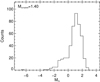Fig. 12.

K_s absolute magnitude (M_{K_s}) histogram of Class II sources in GMF 46 (GMF319.0−318.7).

Robitaille et al. (2006) presented a grid of radiation transfer models of YSOs (∼20 000 YSO models), covering a wide range of stellar masses, disk masses, envelope masses, and accretion rates. For each YSO model, SEDs are calculated for ten inclination angles. The model SEDs are also convolved to commonly used filters to generate broadband fluxes within 50 different apertures (100−100 000 AU). In our analysis, we use the aperture of ∼45 000 AU, corresponding to ∼3″ at a distance of 15 kpc. Using other large apertures do not change our results (Heyer et al. 2016). Robitaille et al. (2006) also defined three evolutionary stages of YSOs based on the accretion rates of envelopes and disks relative to the stellar masses: Stage I has Ṁ_env/M_∗ > 10⁻⁶ yr⁻¹; Stage II has Ṁ_env/M_∗ < 10⁻⁶ yr⁻¹ and M_disk/M_* > 10⁻⁶; and Stage III has Ṁ_env/M_∗ < 10⁻⁶ yr⁻¹ and M_disk/M_* < 10⁻⁶.

Andrews et al. (2013) investigated the disk and stellar masses of Class II sources in Taurus and they found a roughly linear scaling between disk and host star masses, with a typical disk-to-star mass ratio of ∼0.2%−0.6%. We extract the Stage II models with 0.001 < M_disk/M_* < 0.01, 0.08 < M_* < 7 M_⊙, and 30 ° < inclination angle < 60°. Figure 13 shows the distribution of these models in the M_{K_s} − M_* plane. Obviously, there is a correlation between stellar mass and K_s band absolute magnitude for Class II sources. We use a four-order polynomial function to fit the points and then establish a relation between M_{K_s} and M_*. The gray region in Fig. 13 shows the fitting uncertainties (1σ), which is also adopted as the uncertainty of the relation. Fang et al. (2013) investigated the YSOs in L1641 using the optical spectroscopy and estimate the stellar masses of YSOs based on effective temperatures and bolometric luminosities with several different pre-main sequence (PMS) evolutionary models. We plot the K_s absolute magnitudes and stellar masses obtained with Siess et al. (2000) PMS models of the Classic T Tauri stars (CTTS) from Fang et al. (2013) in Fig. 13 with green dots. Most of CTTS are located in the gray region of Fig. 13, which confirms that M_{K_s} − M_* relation for Class II sources established by us is also consistent with the observational results.

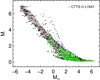Fig. 13.

Relation between stellar mass and K_s absolute magnitude of Class II source. The black dots represent the Robitaille et al. (2006) Stage 2 models with 0.001 < M_disk/M_* < 0.01, 0.08 < M_* < 7 M_⊙, and 30 ° < inclination angle < 60°. The red curve shows the robust polynomial fitting while the gray region shows the 1σ uncertainty of the fitting. The CTTS in L1641 from Fang et al. (2013) are marked with green filled circles.

Using above M_{K_s} − M_* relation, the flux completeness of Class II sources in each GMF can be transfered to mass completeness. The obtained mass completeness (M_comp) of Class II sources in different GMFs are from 0.9 to 4.7 M_⊙, with the average uncertainty of ±0.6 M_⊙.

The number (N_ClassII) of Class II sources brighter than the completeness limit is used to estimate the total number and mass of Class II sources by extrapolating from M_comp down to the hydrogen burning limit (0.08 M_⊙) with the Kroupa IMF (Kroupa 2001).

3.3.2. Mass of Class I populations

Protostars are in the main accretion phase and the luminosities of protostars are also correlated with the accretion process. However, the accretion rate onto a protostar is still under debate (Dunham et al. 2014). On the other hand, the intrinsic stellar parameters of protostars are also poorly constrained. The pre-main sequence evolution, especially during the first few Myr, is much less well constrained (Dunham et al. 2014, and references therein). Therefore, it is difficult to construct a relation between luminosity and mass for Class I sources.

We also extract some Robitaille et al. (2006) Stage I models with 0.001 < M_disk/M_* < 0.1, 0.08 < M_* < 7 M_⊙, 30 ° < inclination angle < 60°, and 10⁻⁸ < Ṁ_disk < 10⁻⁵ (Caratti o Garatti et al. 2012; Antoniucci et al. 2014; Heyer et al. 2016). However, we do not find any correlation between M_* and M_{K_s} for Class I sources. Therefore, in the present work we have tried to use LF to estimate the total number of Class I sources in each GMF.

Kryukova et al. (2012) identified protostars in nine star-forming molecular clouds within 1 kpc and constructed the combined LFs for low-mass star-forming clouds and high-mass star-forming clouds (LLF and HLF hereafter) as shown in Fig. 14. The red vertical lines in Fig. 14 show the luminosity completeness of LLF and HLF (L_cut, LLF and L_cut, HLF). Kryukova et al. (2012) found significant difference between LLF and HLF: HLF peaked near 1 L_⊙ with a tail extending toward luminosities above 100 L_⊙ while LLF peaked below 1 L_⊙ without >100 L_⊙ tail. Assuming the universal LFs for low-mass star-forming regions and high-mass star-forming regions, LLF and HLF constructed by Kryukova et al. (2012) as the templates can be used to estimate the total number of Class I sources in our GMFs.

Fig. 14.

Dereddened luminosity functions constructed by Kryukova et al. (2012) for the combined low-mass star-forming clouds (left) and combined high-mass star-forming clouds (right). The red vertical lines show the dereddened L_cut.

In each GMF, we calculated the bolometric luminosities of Class I sources using the trapezoid rule to integrate over the finitely sampled dereddened SEDs (Dunham et al. 2008, 2015). We find that all our GMFs harbored Class I sources with luminosities of >100 L_⊙, indicating that all our samples are high-mass star-forming molecular clouds. Thus we assume an universal LF that is the same as HLF for all the GMFs.

Because most of Class I sources are identified based on Spitzer photometric catalog (< 20% Class I sources are identified based on emission at 70μm), the luminosity completeness of Class I sources (L_cut) is estimated based on different Spitzer bands. We plot the histograms of photometry at 8 μm and 24 μm for Class I sources in each GMF, and then adopt the peaks as the magnitude completeness (m₈ and m₂₄). Using the method presented by Kryukova et al. (2012), m₈ and m₂₄ can be converted to the luminosity completeness and finally the higher value is adopted as L_cut. Figure 15 shows the dereddened LF of Class I sources in GMF 46 (GMF319.0−318.7) and the corresponding L_cut is marked with the red line.

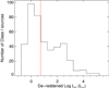Fig. 15.

Dereddened luminosity function of Class I sources in GMF 46 (GMF319.0−318.7). The red vertical line shows the dereddened L_cut.

The number (N_ClassI) of Class I sources brighter than L_cut is used to estimate the total number of Class I sources by extrapolating from L_cut down to L_cut, HLF with HLF template. The L_cut, HLF = 0.055 L_⊙ is similar as L_cut, Orion = 0.047 L_⊙ (Kryukova et al. 2012). The mass completeness of protostars in Orion is about 0.2 M_⊙ (Willis et al. 2013). Thus the total number of Class I sources estimated above is also complete down to ∼0.2 M_⊙. Using the total number of Class II sources that is obtained by extrapolating down to 0.2 M_⊙ with Kroupa IMF, we can calculate the number ratio of Class I to Class II sources, based on which the total number of Class I sources down to 0.08 M_⊙ ( $N_{tot}^{c 1}$ $N_{\mathrm{tot}}^{\mathrm{c1}}$ ) can be estimated. The uncertainty of total number of Class II sources also contribute to the final uncertainty of $N_{tot}^{c 1}$ $N_{\mathrm{tot}}^{\mathrm{c1}}$ . The average uncertainty of log $(N_{tot}^{c 1})$ $(N_{\mathrm{tot}}^{\mathrm{c1}})$ in all GMFs is about ±0.13 dex.

During above calculating process, we assumed an universal LF for all high-mass star-forming molecular clouds. Kryukova et al. (2012) examined the luminosity functions as a function of the local surface density of YSOs in the Orion molecular cloud and they found a significant difference between the luminosity functions of protostars in regions of high and low stellar density, the former of which is biased toward more luminous sources. This result has also been confirmed in the Cygnus-X star-formating complex by Kryukova et al. (2014), indicating the variations of protostellar LF due to the different surrounding environment. Kryukova et al. (2012) constructed two LFs for protostars in the low and high stellar surface density regions of Orion. We found that using different LFs to estimate total number of protostars could introduce an additional uncertainty of about ±0.2 dex to the log $(N_{tot}^{c 1})$ $(N_{\mathrm{tot}}^{\mathrm{c1}})$ , which results in an additional uncertainty of about 0.04 dex to the log(SFR). Assuming a mean mass of 0.5 M_⊙, the total mass of Class I populations can be obtained based on $N_{tot}^{c 1}$ $N_{\mathrm{tot}}^{\mathrm{c1}}$ .

3.3.3. SFRs and SFEs

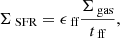
We calculated two estimates for the SFRs of the GMFs based on their YSO content. The first reflects the average SFR during the Class I + Class II lifetimes, and we call this measure simply SFR. The second reflects the average SFR during the Class I lifetime only, and we call this measure the current SFR, or cSFR. Both quantities are calculated by dividing the total mass of YSOs in respective classes by the relevant timescale. We adopted 2 Myr (Evans et al. 2009) and 0.54 Myr (Heiderman & Evans 2015) as the Class I+II and Class I lifetimes, respectively. We also calculated SFE analogously with the SFR with

$\begin{matrix} SFE = \frac{M_{YSO}}{M_{YSO} + M_{cloud}}, \end{matrix}$ $\begin{aligned} {\text{ SFE}} = \frac{M_{\text{ YSO}}}{M_{\text{ YSO}}+M_{\text{ cloud}}}, \end{aligned}$ (3)

where M_YSO is the total mass of Class I + Class II sources in each GMF. Similarly, we calculate the SFE of the dense gas with

$\begin{matrix} {SFE}_{dense} = \frac{M_{YSO}}{M_{YSO} + M_{dense}} \cdot \end{matrix}$ $\begin{aligned} {\text{ SFE}}_{\text{ dense}} = \frac{M_{\text{ YSO}}}{M_{\text{ YSO}}+M_{\text{ dense}}}\cdot \end{aligned}$ (4)

There are 11 GMFs that have too few Class I or Class II sources to estimate the total mass of YSOs, of which ten GMFs are located at the distances of >8 kpc and one GMF (GMF 10, i.e., F24 in Table H.1) has only four Class I sources with the luminosities of >L_cut although it is located at a distance of 4.7 kpc. We also note that the dense gas mass fraction (M_dense/M_cloud) of GMF 10 is only ∼0.4%. Therefore, we finally obtain the SFRs and SFEs for only 46 GMFs. The uncertainties of SFRs and SFEs are from the uncertainties of total mass of YSOs. We obtain the probability distributions of SFRs and SFEs with a Monte Carlo method and use these distributions to define the uncertainties (see Appendix D). The uncertainty introduced due to the variations of protostellar LF during estimating the total mass of Class I sources is not included. Table H.2 shows the SFR and SFE obtained for each GMF. We note that the uncertainties listed in Table H.2 do not include the distance uncertainty (see Appendix D for details).

Even though we have excluded some contamination from the identified YSO population (see Sect. 3.2.4), YSOs on the background of the cloud, possibly associated with other molecular clouds along the line of sight, may still contaminate the total YSO estimate. Specifically, the SFRs and SFEs could be overestimated for the GMFs that exhibit other CO velocity components, and thus possibly other star-froming regions, along the line of sight. We checked each GMF and flagged the ones that are overlapped with other GMFs (Table H.2). We also examined the ¹³CO average spectrum of each GMF and calculated the flux ratio of GMF to other velocity components. High flux ratio implies that the GMF is the dominating component along the line of sight. We used this ratio as a parameter (R) as one measure of the reliability of obtained SFR and SFE. We note that we did not obtain the R value for Nessie due to the lack of sensitive ¹³CO data. Figures 3–9 (right panels) show the ¹³CO average spectra for seven GMFs with R > 1.

All above calculations of SFRs and SFEs are based on the assumption that the identified YSOs are individual objects. Obviously, the presence of unresolved clustering are not accounted for in our estimations. However, Morales & Robitaille (2017) analyzed near-infrared UKIDSS observations of a sample of GLIMPSE-selected YSO candidates in the Galactic plane (Robitaille et al. 2008) and found that ∼87% of YSO candidates have only one dominant UKIDSS counterpart. Based on this, Morales & Robitaille (2017) suggested that the YSO clustering within the GLIMPSE resolution is not important for the GLIMPSE-selected YSOs with intermediate to high masses, and hence, no significant corrections are needed for estimates of the SFR based on the assumption that the GLIMPSE YSOs are individual objects. In our YSO sample, ∼80% are identified based on the Spitzer data while ∼20% are selected using AllWISE and Herschel Hi-GAL data with the spatial resolution of ∼6″. To estimate the possible influence of YSO clustering on our SFRs, we inspect a worst-case scenario in which all YSOs identified using AllWISE and Herschel data are in fact YSO clusters. Gutermuth et al. (2009) investigated 36 nearby YSO clusters and found that a typical young cluster has 26 members with a surface density of 60 pc⁻². Thus each AllWISE or Hi-GAL selected YSO can be decomposed into several members within the resolution of 6″ based on its distance, and then “intrinsic” number of YSOs can be obtained for each GMF. We found that the YSO clustering has small influence on the SFR estimates for the GMFs located at the distances of <4.5 kpc. However, for the GMFs with the distances of >4.5 kpc, we could significantly underestimate the SFRs by a factor of 1.5–7. For the GMFs with the distance of <5.5 kpc, we could underestimate the SFRs within a factor of up to two.

4. Results

4.1. Gas properties of the GMFs

Figure 16 shows the spatial distribution of 57 GMFs. We indicated their positions on the ¹³CO integrated intensity images of the GRS and ThrUMMS survey data with the red ellipses.

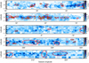Fig. 16.

Spatial distribution of 57 Galactic GMFs. The backgrounds are ¹³CO intensity maps of the GRS and ThrUMMS data, integrated over the entire observed velocity range. The red ellipses mark the positions of 57 GMFs. We obtained the star formation rates of 46 GMFs (see Sect. 3.3 for details) that are labeled with green pluses.

Figure 17 shows the distributions of physical parameters of 57 GMFs. We note that Zucker et al. (2018) also perform a systematic reanalysis of the physical propertites of about 45 giant filaments selected from literature. However, they use Herschel Hi-Gal survey data to estimate the column densities and dust temperatures of the giant filaments. To match the filamentary structures identified in the corresponding original studies, they delineate different boundaries for different giant filaments rather than applying a same column density threshold to all objects. Therefore, we did not perform a direct comparison of our filament parameter estimates to that of Zucker et al. (2018).

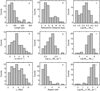Fig. 17.

Distributions of filament length (panel a); heliocentric distance (panel b); logarithm of cloud mass M_cloud (panel c); line width Δv (panel d); logarithm of gas surface density Σ_gas (panel e); logarithm of dense gas mass M_dense (panel f); free-fall time obtained based on spherical morphology (panel g); aspect ratio (panel h); and logarithm of dense gas mass per unit length (panel i).

The median length of 57 GMFs is 67 pc, with a minimum of 17 pc and a maximum of 268 pc, where the length of GMFs is defined as the major axis obtained through fitting the column density map of a GMF with an ellipse (see Sect. 3.1). For the samples originally identified by Ragan et al. (2014), Wang et al. (2015), and Abreu-Vicente et al. (2016) based on the same GRS and ThrUMMS data, the lengths estimated using our method described in Sect. 3.1 are similar as that given by the corresponding papers. However, for the samples originally identified by Li et al. (2016) and Wang et al. (2016) based on the dense gas tracers, the lengths estimated using ¹³CO data with our method are significantly longer. Zucker et al. (2015) mainly focus on the dense part of the giant filament and the lengths given by them are usually shorter than the lengths obtained by us. The heliocentric distances of 57 GMFs are in the range of [2,13] kpc, with a median value of 5.1 kpc. 35 (∼61%) of 57 GMFs are located at the distances of <5.5 kpc and 22 (∼39%) are located at the distances of <4.5 kpc.

To provide a rough description of the GMF shapes, we compute the ratio of the major to minor axis of the ellipses that were fit to the column density maps of the GMFs and obtain the values are between 1–6.7 with the median value of ∼2. We call this value an “aspect ratio”, however, we immediately emphasize that an ellipsoid is not a good approximation of the morphology of the GMFs; a cylindric model that identifies and traces the crest of the filament would be more accurate. Such definition is beyond this paper; our goal is only to provide a simple descriptive statistic. As a result of this definition, our aspect ratios are smaller than given for filaments in the literature by works that adopt more refined techniques to describe the filamentary morphology (e.g., Wang et al. 2015, 2016; Zucker et al. 2018). Some works in literature studying molecular clouds in general have adopted a description of molecular cloud shapes that is similar to ours. For example, Miville-Deschênes et al. (2017) uses a similar technique to describe shapes of giant molecular clouds (GMCs). They find an average aspect ratio of ∼1.5 for all GMCs, a value which is slightly smaller than the median aspect ratio of our GMFs. An interpretation of this is that our aspect ratio reflects mostly the elongation of the relatively low column density GMC inside which the denser gas shows a high-aspect ratio, filamentary morphology.

We obtained the average ¹³CO line width (Δv) of each GMF based on its moment two map (see Appendix B). Table H.1 lists the values of Δv for 56 GMFs (except Nessie). These values are in the range of [1.6, 5.9] km s⁻¹ with a median value of 3.4 km s⁻¹. Evans et al. (2014) compiled a list of linewidths for ∼29 nearby molecular clouds and they obtained the median linewidth of 1.5 km s⁻¹, with a minimum of 0.8 km s⁻¹ and a maximum of 3 km s⁻¹. The value of 3.4 km s⁻¹ is almost twice of the median linewidth of nearby low-mass star-forming regions, however, similar to the median value of ∼4 km s⁻¹ estimated in the IRDCs (Simon et al. 2006; Du & Yang 2008). This is not surprising because most of GMFs are also identified based on the IRDCs.

The median values of M_cloud and Σ_gas are 1.5 × 10⁵M_⊙ and 128 M_⊙ pc⁻², respectively, which are slightly lower than the typical values of the local giant molecular clouds (∼2 × 10⁵M_⊙ and ∼170 M_⊙ pc⁻²; Solomon et al. 1987). We note that we use the extinction contour of A_V = 3 mag to estimate the cloud mass, which is inclined to underestimate the total mass of the GMFs.

In Fig. 18, we show the line widths (Δv) versus the sizes (R) and masses (M_cloud). Here the size is the equivalent radius obtained using the area of the GMFs. The error bars in this and the subsequent figures include distance errors (see Appendix D for details). We first tested the relationships for correlations without considering the uncertainties and find significant correlations between Δv and R, M_cloud with Pearson r = 0.67 for Δv versus R and 0.71 for Δv versus M_cloud. As a comparison, a significant (3σ) correlation requires Pearson $| r | > 3 / \sqrt{N_{s} - 1}$ $|r| > 3/\sqrt{N_{\mathrm{s}}-1}$ where N_s is the sample size (56 here) (Vutisalchavakul et al. 2016). The direct least-square linear fitting without considering uncertainties gives the slopes of 0.35 ± 0.05 for Δv versus R and 0.17 ± 0.02 for Δv versus M_cloud. We then calculate the linear regression coefficients using the Bayesian method developed by Kelly (2007) that allows the inclusion of uncertainties along both axes during the fitting process. We note that the fitting routine requires symmetric uncertainties; for asymmetric uncertainties we simply used the maximum of the two asymmetric errors. Based on the posterior distributions as shown in the inset plots of Fig. 18, the 95% confidence intervals of correlation coefficients are about [0.65, 1.0] for Δv versus R and [0.61, 1.0] for Δv versus M_cloud, respectively. These indicate significant correlations between Δv and R, M_cloud. The posterior median estimates of the slopes are 0.42 ± 0.10 for Δv versus R and 0.22 ± 0.06 for Δv versus M_cloud, individually, which are slightly larger than the slopes obtained without considering uncertainties. These values are also consistent with the canonical relationships obtained by Larson (1981) and Solomon et al. (1987).

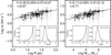Fig. 18.

¹³CO line widths vs. sizes (left panel) and masses (right panel) of the GMFs in log-log plane. The solid lines show the best linear fittings to the points without considering the uncertainties. The correlation coefficients and the fitting results that are obtained without considering the uncertainties are also marked in the top region of panels. The small inset plots in each panel show the probability distributions of correlation coefficients and fitting slopes that are obtained after including uncertainties on both axes using the Bayesian linear regression method developed by Kelly (2007).

4.2. Observed YSO content of GMFs

Table H.2 lists the number of Class I and Class II sources detected in each GMF. In total, we identified 18 395 YSOs (ClassI+II) in 46 GMFs and ∼38% of the YSOs are Class I sources.

The spatial distribution of YSOs is a powerful diagnostic of their formation and early evolution (Kraus & Hillenbrand 2008). We next consider briefly the spatial distribution of the YSOs. We only discuss the Class I sources, because they are still possibly close to their formation sites due to their short lifetime (Lada et al. 2013). The investigation of the clustering of stars at the time of their formation is helpful to establish the connections between the star formation process and the molecular cloud structures.

The degree of clustering of protostars can be quantified with the two-point correlation function (TPCF). In this part, we describe our calculation of the TPCF using the estimator presented by Landy & Szalay (1993), following the method suggested by Kainulainen et al. (2017, see their Sect. 3.3 for details). The TPCF, ξ(r), describes the excess probability distribution of the sources with different separations (r) comparing to a random distribution. The ξ(r) = 0 indicates that the distribution can not distinguish from a random distribution while ξ(r)> 0 and ξ(r)< 0 indicate excess and deficit of separations, individually. We only used the Class I sources with the luminosities higher than the luminosity completeness (L_cut) that is obtained in Sect. 3.3.2 to calculate the TPCF in each GMF. We finally obtained the TPCFs of Class I sources in six “reliable” GMFs that have R > 1, $N_{obs}^{c1}$ $N_{\text{ obs}}^{\text{ c1}}$ (>L_cut) >50, distance <4.5 kpc, and are not overlapped with other GMFs based on in total 1683 Class I sources. Figures 4–9 show the spatial distributions of Class I sources in these six GMFs and Fig. 19 shows the TPCFs.

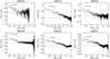Fig. 19.

Two-point correlation functions for the Class I sources in 6 GMFs. The title on each panel corresponds to the ID number of Table H.2. The red solid lines show the linear fits to the roughly straight line part of the data and the fitting slopes are labeled in each panel.

The TPCFs of Class I sources in these six GMFs show 1) obvious clustering of protostars at the small stellar separations; 2) a monotonous decrease with stellar separations in the clustering regime. We try to fit the linear part of TPCFs with a single power law. The obtained power law indices (α) are from −0.58 to −0.20.

The power law TPCFs of YSOs have been observed in some Galactic and extragalactic star-forming regions and are usually interpreted as hierarchical or fractal distributions that could be related to the hierarchical structures of the gas (Gomez et al. 1993; Larson 1995; Simon 1997; Kraus & Hillenbrand 2008; Gouliermis et al. 2014; Koenig & Leisawitz 2014). The power law index is also related to the 2D fractal dimension D₂ as D₂ = α + 2 (Larson 1995). Therefore, the single power law TPCFs in our samples can be also interpreted as fractal clustering of YSOs with the fractal dimensions of D₂ ∼ 1.42−1.80. We note that this range of D₂ is consistent with the range of D₂ ∼ 1.2−1.9 that is obtained in the nearby star-forming regions (Nakajima et al. 1998; Alfaro & Sánchez 2011).

4.3. Star formation rates and efficiencies

Table H.2 lists the SFRs and SFEs obtained for 46 GMFs. Due to the large uncertainties of SFR estimations for the distant GMFs (see Sect. 3.3.3), in this section we apply the statistical analysis to only the 34 GMFs with the distances of <5.5 kpc.

Figure 20 shows the combined probability distributions of SFR, SFE, and Σ_SFR (see Appendix D) for these 34 GMFs. The median values of SFR, Σ_SFR, and SFE for these 34 GMFs are 630 M_⊙ Myr⁻¹, 0.62 M_⊙ Myr⁻¹ pc⁻², and 1%, individually.

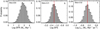Fig. 20.

Probability distributions of star formation rate (panel a); star formation efficiency (panel b); surface density of star formation rate for 34 GMFs with the distances of <5.5 kpc (panel c). The red vertical lines show the median values of SFE and Σ_SFR that are re-estimated with Class I+Flat+II sources in the nearby star-forming regions (see the text for details).

Evans et al. (2009) obtained the Σ_SFR in five nearby star-forming regions and found that the values of Σ_SFR are in the range of 0.65−3.2 M_⊙ Myr⁻¹ pc⁻², with a median value of 1.3 M_⊙ Myr⁻¹ pc⁻². Evans et al. (2014) re-investigated the star formation rates in 29 nearby star-forming clouds and obtained Σ_SFR in the range of 0.06−3.88 M_⊙ Myr⁻¹ pc⁻² with a median value⁸ of 0.9 M_⊙ Myr⁻¹ pc⁻². The SFEs obtained in five nearby star-forming clouds by Evans et al. (2009) are ∼3−6%, with a median value of ∼5%. Based on a larger sample, Evans et al. (2014) found that SFEs in nearby star-forming regions are in the range of [0.2%, 7.8%], with a median value of 1.8%. At a first glance, the Σ_SFR and SFEs of the GMFs are on average significantly lower than that of the molecular clouds in the Gould Belt. However, we must remind that there is a systematic difference between the SFRs obtained in the GMFs and nearby star-forming regions due to the different methods that are used to estimate the SFRs.

Evans et al. (2009, 2014) use all YSOs detected in the nearby star-forming regions to estimate the SFRs, including Class I, Flat, Class II, and Class III sources. However, due to the lack of strong infrared excess, the Class III sources could be incomplete in some clouds. Moreover, the optical spectroscopical observations in Serpens and Lupus found that ∼40−100% of Class III sources are actually background AGB stars (Oliveira et al. 2009; Romero et al. 2012). Considering the high contamination fraction in the Galactic plane, we only use Class I+Flat and Class II sources detected in the GMFs to estimate the total number of YSOs.

To compare the GMFs with nearby star-forming regions, we recalculate the SFRs of the nearby clouds based on the latest version of YSO samples in the c2d and Gould Belt surveys presented by Dunham et al. (2015). We obtain the extinction map for each nearby molecular cloud with 2MASS (Skrutskie et al. 2006) point source catalog using PNICER (Meingast et al. 2017) that is an improved version of the well-known NICER and NICEST algorithms (Lada et al. 1994; Lombardi & Alves 2001; Lombardi 2009), providing a suite for measuring extinction toward individual sources and producing extinction maps with an unsupervised machine learning algorithm. The uncertainties of extinction maps are mainly from the 2MASS photometric uncertainties and the scatters of intrinsic colors. We use the extinction contour of A_V = 3 mag to define the boundaries of nearby molecular clouds and the gas mass and dense gas mass are obtained through integrating down to A_V = 3, and 7 mag in 2MASS extinction maps. The uncertainties of mass estimates are mainly from the uncertainties of extinction maps and distances. SFRs of nearby clouds are estimated with Class I+Flat+II sources within the cloud boundaries based on the relation of SFR = 0.25N(YSOs)M_⊙ Myr⁻¹. The uncertainties of SFRs are based on counting statistics. We used the method suggested by Evans et al. (2014) to estimate the uncertainties of the parameters of nearby clouds. The details about this method can be found in the Appendix B of Evans et al. (2014).

Table 3 lists the SFRs obtained in 24 nearby molecular clouds. The median values of SFEs and Σ_SFR in the nearby star-forming regions are 1.1% and 0.64 M_⊙ Myr⁻¹ pc⁻², respectively, which are also marked with red vertical lines in Fig. 20. Therefore, on average, the SFE and Σ_SFR in the GMFs are similar to that in nearby star-forming regions. However, there could still be systematic differences for SFE because we use ¹³CO-based column density maps and extinction maps to estimate M_cloud for the GMFs and nearby star-forming regions, respectively. Ripple et al. (2013) compared the column density distribution derived using dust extinction with that derived using ¹³CO emission in the Orion molecular cloud. They find that ¹³CO provided a reliable tracer of H₂ mass within the area with strong self-shielding (A_V > 3 mag). However, Ripple et al. (2013) used ¹²CO data to estimate the excitation temperature and then combined the excitation temperature measurements with the ¹³CO emission to derive the column densities, which means that they used a slightly more refined method compared to ours (described in Sect. 3.1). Therefore, it is not clear if their conclusion applies as such to the masses we derive. We cannot totally exclude the caveat of systematic differences in the M_cloud and SFE values for GMFs and nearby clouds.

Table 3.

Properties of nearby molecular clouds.

Most of the GMFs are associated with the spiral arms of the Milky Way (Wang et al. 2015, 2016; Zucker et al. 2015; Abreu-Vicente et al. 2016; Li et al. 2016). The nearby star-forming clouds appear to be located in an inter-arm branch between two major spiral arms of the Galaxy (Xu et al. 2013; Molinari et al. 2014). Whether the spiral arms trigger the star formation is still under debate. Based on the extragalactic observations, some studies suggested that there are significant enhancements of star formation in the spiral arms (Seigar & James 2002; Silva-Villa & Larsen 2012), but some other studies found no significant difference for star formation efficiencies in the spiral arm and inter-arm regions (Foyle et al. 2010; Wall et al. 2016). In the Milky Way, several studies also found no significant difference of star formation properties in Galactic spiral arm and inter-arm regions (Eden et al. 2013; Ragan et al. 2016). Our results favor the interpretation that the star formation activities in the spiral arm and inter-arm regions are similar.

Recently, Duarte-Cabral & Dobbs (2017) investigated the evolution of GMFs using a high-resolution section of a spiral galaxy simulation. They found that the GMFs are only detected in the inter-arm regions and are pressure confined rather than gravitationally bounded as a whole. In their simulation, when the GMFs enter into the spiral arm regions, they begin to break into short filament sections due to the stellar feedback from star formation or differential force from the gravitational potential. Duarte-Cabral & Dobbs (2017) did not find a significant increase of star formation events once the GMFs enter the spiral arm, at least in their selected GMF sample. Based on this scenario, we would expect the similar star formation activity between the GMFs in spiral arm regions and the molecular clouds in inter-arm regions.

5. Discussion

5.1. Star formation relations

We next consider the relationships between the star formation and gas properties in the GMFs and compare them with those from the literature. We only include in the analysis the 34 GMFs with distances less than 5.5 kpc. In some analyses below, we consider two separate samples: GMFs and GMFs + nearby clouds. However, our conclusions are mainly based on GMFs alone, because of the possibility that there may be systematic differences between the physical parameters, such as gas mass and free-fall time, of the GMFs and nearby clouds. To minimize this possibility, we have re-derived the parameters that are listed in Table 3 for the nearby clouds, following a procedure similar to the GMFs (see Sect. 4.3 for details). To search for correlations between the parameters, we always use two methods: 1) the Pearson correlation coefficient (does not considering uncertainties); 2) Bayesian linear regression method that makes use of uncertainties along both axes (Kelly 2007).

Figure 21 (panel a) shows the relationship between Σ_SFR and Σ_gas for the GMFs and nearby star-forming clouds. The figure also shows the relations derived by Kennicutt (1998) and Bigiel et al. (2008). The GMFs fall slightly above these relations (as do the nearby star-forming regions, cf., Heiderman et al. 2010). Without considering uncertainties, we find Pearson r values of 0.08 and 0.40 for GMFs and GMFs + nearby clouds, respectively. We note that a significant correlation needs r > 0.52 for GMFs (N_s = 34) and r > 0.40 for GMFs + nearby clouds (N_s = 58). If considering uncertainties, the Bayesian linear regression method (Kelly 2007) can give the posterior distributions of correlation coefficients as shown in the inset plots of Fig. 21. The 95% confidential intervals of correlation coefficients are [−0.9, 0.9] for GMFs and [0.11, 0.77] with a median value of 0.51 for GMFs + nearby clouds. Thus, there are no convincing correlations between Σ_SFR and Σ_gas for GMFs, but there could be a weak correlation for GMFs + nearby clouds.

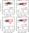Fig. 21.

Surface density of SFR, Σ_SFR, as a function of Σ_gas (panel a), Σ_gas/t_ff, s (panel b), Σ_gas/t_cross (panel c), and Σ_gas/t_ff, f (panel d) for the Galactic GMFs (black filled circles) and the nearby star-forming regions (red triangles). The lines in panel a correspond to the star formation relations suggested by Kennicutt (1998, green solid) and Bigiel et al. (2008, blue dashed). The lines in panels b and d correspond to star formation law suggested by Krumholz et al. (2012) with ϵ_ff = 0.001, 0.01, and 0.1, respectively. The Pearson correlation coefficients between the different sets of parameters obtained without considering uncertainties are marked on top region of each panel and the black fonts are for GMFs while the red fonts are for GMFs + nearby clouds. The inset plots in each panel show probability distributions of correlation coefficients (r) obtained with Bayesian linear regression method by Kelly (2007) for GMFs (black line) and GMFs + nearby clouds (red line).

Next, we discuss the relation between star formation and gas surface density calculated per various timescales. Krumholz et al. (2012) consider a volumetric star formation law, 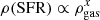$ρ (SFR) \propto ρ_{gas}^{x}$ $\rho ({\rm{SFR}}) \propto \rho _{{\rm{gas}}}^x$ , in which the SFR is proportional to the gas mass per free-fall time (i.e., x = 1.5). Because the volume density is difficult to measure, they only consider the projected quantities:

$\begin{matrix} Σ_{SFR} = ϵ_{ff} \frac{Σ_{gas}}{t_{ff}}, \end{matrix}$ $\begin{aligned} \Sigma _{\text{ SFR}} = \epsilon _{\text{ ff}}\frac{\Sigma _{\text{ gas}}}{t_{\text{ ff}}}, \end{aligned}$ (5)

where ϵ_ff is a dimensionless measure of SFR (i.e., SFR_ff). Krumholz et al. (2012) found that a set of SFR measurements, from nearby star-forming regions to distant sub-millimeter galaxies, can be well fitted by this relation when ϵ_ff∼1%. We plot Σ_SFR versus Σ_gas/t_ff, s and Σ_gas/t_ff, f in Fig. 21 (panels b and d) for GMFs and GMFs + nearby clouds, where t_ff, s and t_ff, f are free-fall time calculated based on spherical and filamentary morphology assumptions (see Appendix B), respectively. Most of GMFs and nearby star-forming regions are located between ϵ_ff= 0.001 and 0.1. The mean values of SFR_ff, s and SFR_ff, f are 0.02 and 0.03 for the GMFs, respectively. These values are higher than the value of 0.01 obtained by Krumholz et al. (2012). We find no convincing correlation between Σ_SFR and Σ_gas/t_ff for GMFs. However, there could be also a weak correlation between Σ_SFR and Σ_gas/t_ff for GMFs + nearby clouds.

The crossing time of molecular clouds can be hypothesized to be a relevant timescale, replacing the t_ff in the volumetric star formation law. Evans et al. (2014) defined $t_{cross} = \frac{size}{⟨ Δ v ⟩}$ $t_{\mathrm{cross}} = \frac{size}{\langle \Delta \mathit{v} \rangle}$ , where size is the equivalent diameter and ⟨Δv⟩ is the mean linewidth of the molecular clouds. They find no significant correlation between Σ_SFR and Σ_gas/t_cross for the nearby star-forming regions. Figure 21 (panel c) shows the relation between Σ_SFR and Σ_gas/t_cross for the GMFs and nearby star-forming regions. We do not find a significant correlation between Σ_SFR and Σ_gas/t_cross for GMFs or GMFs + nearby clouds.

We note here as a caveat that although we do not detect convincing correlations between Σ_SFR and Σ_gas, Σ_gas/t_ff or Σ_gas/t_cross for GMFs, this does not mean that there is no possibility of strong correlations between these quantities. If we see the posterior distributions of correlation coefficients obtained with Bayesian linear regression method (Kelly 2007) for GMFs in Fig. 21 (inset plots), they are close to a uniform distribution rather than a distribution peaked at zero. In other words, the uncertainties of Σ_SFR, Σ_gas, Σ_gas/t_ff, and Σ_gas/t_cross in GMFs are too large to decide whether there are correlations between them.

Another star formation relation that highlights the role of dense gas has been developed. This relation originates from the works of Solomon & Sage (1988) and Gao & Solomon (2004), based on the investigation of galaxies, which suggests that the SFR traced by infrared luminosity is tightly correlated with dense gas traced by HCN luminosity. Wu et al. (2005) found that this relation can be extended to the Galactic dense cores, indicating a global star-forming law from local star-forming regions to the distant galaxies. Kainulainen et al. (2009) show that the solar neighborhood clouds with a higher number of YSOs systematically have a higher relative amount of gas at high column densities. Lada et al. (2010) investigated the star formation activity in several nearby clouds and found that the SFR estimated with the YSO counting method correlates best with specifically the mass at high column densities (A_K > 0.8 mag), which is agreement with the star formation relation suggested by Solomon & Sage (1988), Gao & Solomon (2004), and Wu et al. (2005). Shimajiri et al. (2017) found that this linear SFR−M_dense relation obtained in the nearby clouds can be also extended to the external galaxies after improving the dense gas mass estimates of external galaxies with a new HCN conversion factor, which indicates a quasi-universal star formation efficiency in the dense molecular gas of galaxies on a wide range of scales. Lada et al. (2012) argued that their star formation law is only compatible with the above volumetric law (Krumholz et al. 2012) if x = 1 and ρ_gas > ρ_th, where ρ_th is a volume density threshold that roughly corresponds to the surface density threshold of A_K = 0.8 mag. Kainulainen et al. (2014) showed that also the volume density of gas follows these relations, meaning that the relative amount of gas at high volume densities correlates with the SFR of the clouds; this directly evidences a volumetric star formation law and the impact of dense gas for star formation.

Our results enable extending the above analyses from the Solar neighborhood to a wider, Galactic context. As a caveat, we note again that we derive the dense gas mass by integrating the ¹³CO-based extinction maps down to A_V = 7 mag. However, it is possible that ¹³CO is not a good tracer of dense gas due to the optical depth effects and depletion (Pineda et al. 2008; Goodman et al. 2009). Compared with the mass estimates in nearby clouds based on the near-infrared extinction mapping, we could significantly underestimate the dense gas mass for the GMFs. To avoid problems due to this, we used only GMFs to investigate the star formation relations rather than combine the GMFs and nearby clouds together in the subsequent part.

Figure 22 shows the relation between SFR and M_dense (panel a) and the relation between SFR and M_cloud (panel b) for the GMFs. There are strong correlations for SFR versus M_dense and SFR versus M_cloud for the GMFs. With Bayesian linear regression method considering uncertainties (Kelly 2007), we also obtain the probability distributions of intrinsic scatters (σ) for SFR−M_dense and SFR−M_cloud relations. The posterior median estimates of σ are 0.12 ± 0.07 for both SFR−M_dense and SFR−M_cloud relations. Thus, we do not find a better correlation of SFR with the dense gas mass than with the total cloud mass, as found by Lada et al. (2010). This difference quite possibly originates from different definitions of the total gas mass; we use the level of A_V = 3 mag to define boundaries of molecular clouds, while Lada et al. (2012) uses ∼1 mag. Indeed, we reanalyzed the nearby clouds using a higher threshold for total gas (see measurements in Table 3) and found significant correlations between SFR and M_{dense, A_V > 7}, M_{cloud, A_V > 3}. The intrinsic scatters are 0.37 ± 0.08 for SFR−M_dense relation and 0.46 ± 0.10 for SFR−M_cloud. In conclusion, the SFR does not correlate better with dense gas mass than the total gas mass in nearby clouds either, if we use A_V = 3 mag to define the boundary of the clouds.

Fig. 22.

SFR and Σ_SFR as a function of dense gas mass (panel a); cloud mass (panel b); and f_DGΣ_gas for GMFs (panel c). The GMFs from different original identification publications are marked with different symbols. The abbreviations correspond to the column one of Table 2. The straight lines represent Lada’s equation (green solid line, Lada et al. 2010), the relation from Wu et al. (2005; blue dashed line), fitting result from Evans et al. (2014; red dotted line), and our linear fitting results without considering uncertainties (black solid line). The Pearson correlation coefficients between the different sets of parameters obtained without considering uncertainties are marked on top region of each panel. The inset plots in each panel show the probability distributions of correlation coefficients (r), fitting slopes, and intrinsic scatters (σ) obtained with Bayesian linear regression method by Kelly (2007).

It is possible that including information on the dense gas would improve the correlation between the Σ_SFR and surface density of gas discussed earlier (Fig. 21, panel a). The SFR−M_dense relation can be transformed into a relation in the Σ_SFR − Σ_gas plane by introducing a parameter f_DG = M_dense/M_cloud (Lada et al. 2012). Figure 22 (panel c) shows the relation between Σ_SFR and f_DGΣ_gas for the GMFs. The Pearson r (does not consider uncertainties) is 0.18. Using the Bayesian linear regression method by Kelly (2007), the 95% confidential interval of the correlation coefficient is [−0.4, 0.9] with a median value of 0.33. Thus we find no significant correlation between Σ_SFR and f_DGΣ_gas for GMFs. However, due to the large uncertainties we can not exclude the possibility that there is a correlation between Σ_SFR and f_DGΣ_gas for GMFs.

Overall, the star formation rate per free-fall time of GMFs is in the range of 0.002−0.05 with a median value of 0.02, which is roughly consistent with the results of Krumholz et al. (2012). However, the large uncertainties of Σ_SFR, Σ_gas, f_DGΣ_gas, and Σ_gas/t_ff do not allow us to obtain any robust conclusion about whether there are correlations between these parameters; for this purpose, more accurate measurements of SFR and gas mass are needed. Covering wider dynamic ranges of the parameters would also be helpful in studying the relationships. However, we detect a significant correlation between SFR and M_dense for GMFs, which indicates that the gas mass above a visual extinction of 7 mag can be used as a predictor of SFR.

5.2. SFR control factors of the molecular clouds

In the previous section we found a strong correlation between SFR and gas mass for GMFs. The Bayesian linear regression gives the relationship

$\begin{matrix} SFR (M_{⊙} {Myr}^{- 1}) \propto M_{dense}^{(0.66 \pm 0.12)} (M_{⊙}) . \end{matrix}$ $\begin{aligned} {\text{ SFR}}\, (M_{\odot }\,{\text{ Myr}}^{-1}) \propto M_{\text{ dense}}^{(0.66 \pm 0.12)}\, (M_{\odot }). \end{aligned}$ (6)

This is shallower than the approximately linear relationship found in the nearby clouds (Lada et al. 2010)

$\begin{matrix} {SFR}_{Lada} (M_{⊙} {Myr}^{- 1}) = 0.046 M_{dense} (M_{⊙}), \end{matrix}$ $\begin{aligned} {\text{ SFR}_{\text{ Lada}}}\, (M_{\odot }\,{\text{ Myr}}^{-1})=0.046 M_{\text{ dense}}\,(M_{\odot }), \end{aligned}$ (7)

or in the Galactic dense cores (Wu et al. 2005)

$\begin{matrix} {SFR}_{Wu} (M_{⊙} {Myr}^{- 1}) = 0.012 M_{dense} (M_{⊙}) . \end{matrix}$ $\begin{aligned} {\text{ SFR}}_{\text{ Wu}}\, (M_{\odot }\,{\text{ Myr}}^{-1})=0.012 M_{\text{ dense}}\, (M_{\odot }). \end{aligned}$ (8)

The slope we derive is closer to that derived by Evans et al. (2014), who reinvestigated the SFRs in the nearby star-forming regions with a uniform YSO sample. They obtain a relation of

$\begin{matrix} {SFR}_{Evans} (M_{⊙} {Myr}^{- 1}) = 0.041 M_{dense}^{0.89} (M_{⊙}) . \end{matrix}$ $\begin{aligned} {\text{ SFR}}_{\text{ Evans}}\, (M_{\odot }\,{\text{ Myr}}^{-1})=0.041 M_{\text{ dense}}^{0.89} (M_{\odot }). \end{aligned}$ (9)

However, the role of uncertainties in the parameters of Eqs. (7)–(9) is unclear and thus it is not possible to address the significance of the differences between Eq. (6) and Eqs. (7)–(9).

Evans et al. (2014) do not find a significant correlation in SFR/M_dense versus M_dense data (see their Fig. 6), which suggests a linear relationship, in agreement with Lada et al. (2010). We also investigated the relationship between SFR/M_dense and M_dense in the GMFs (Fig. 23). There is a significant negative correlation between SFR/M_dense and M_dense for GMFs. The 95% confidential interval of correlation coefficient obtained with Bayesian linear regression method by Kelly (2007) is [−1, −0.67]. Therefore, the SFR−M_dense relation in GMFs could be a sub-linear rather than a linear relation. We also investigated this relation using different sub-samples such as the GMFs with distances of <3.5, 4, and 5 kpc or GMFs with R > 1 and found that the slopes of SFR−M_dense relations are <1 (considering 1σ uncertainties) in all cases (see Appendix E for details), which confirms that the detection of this approximate sub-linear SFR−M_dense relation in GMFs is not due to sample selection effects. However, we emphasize that the SFR−M_dense relation detected in GMFs is still roughly consistent with the relations suggested by Wu et al. (2004), Lada et al. (2010), Evans et al. (2014) if considering 3σ uncertainties of the slope.

Fig. 23.

SFR/M_dense as a function of dense gas mass for the GMFs. GMFs from different original identification publications are marked with different symbols. The abbreviations correspond to the column one of Table 2. The Pearson r obtained without considering uncertainties is marked on the top of the figure. The inset plots show the probability distributions of correlation coefficient and fitting slope obtained with Bayesian linear regression method by Kelly (2007).

We briefly speculate about the role of filamentary morphology in the star formation of GMFs. We note that in this work, we have not defined the length of the GMFs accurately; we have only measured the length of the GMFs through the fit of an ellipsoid to the column density map of the GMF. For cylindrical structures, the mass per unit length, or line mass, is an important parameter that is linked to the physical state of the filament (e.g., Stodólkiewicz 1963; Ostriker 1964; Fiege & Pudritz 2000; Fischera & Martin 2012; Recchi et al. 2014). With this in mind, we investigated the line density relation between star formation and dense gas, i.e., SFR/L vs. M_dense/L, as shown in Fig. 24 (panel a). L represents the length of clouds that is the major axis obtained through fitting the extinction map of a cloud with an ellipse. We find a significant correlation between the line densities of star formation rate and dense gas mass. The correlation coefficients are 0.72 without considering uncertainties. If considering uncertainties, the 95% confidential interval of correlation coefficient obtained with the Bayesian linear regression method is [0.58, 0.99]. For all data points, we obtain the relation

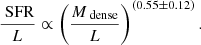
$\begin{matrix} \frac{SFR}{L} \propto {(\frac{M_{dense}}{L})}^{(0.55 \pm 0.12)} . \end{matrix}$ $\begin{aligned} \frac{{\text{ SFR}}}{L} \propto \left(\frac{M_{\text{ dense}}}{L} \right)^{(0.55 \pm 0.12)}. \end{aligned}$ (10)

Fig. 24.

SFR per unit length vs. dense gas mass per unit length for GMFs. GMFs from different original identification publications are marked with different symbols. The abbreviations correspond to the column one of Table 2. The black line shows the linear fittings obtained without considering uncertainties. The Pearson r obtained without considering uncertainties is also marked on the top of the figure. The inset plots show the probability distributions of correlation coefficient and fitting slope obtained with Bayesian linear regression method by Kelly (2007).

In the context of GMCs in general, it has been found that the internal structure, or morphology, plays an important role in predicting the SFRs of GMCs. For instance, Lada et al. (2013, 2017) investigated the star formation activity in several well-studied local molecular clouds and found that the number of protostars is correlated with the area of the cloud above a given extinction A_K, denoted as S′(A_K). Obviously, S′(A_K) reflects the cloud structure. Kainulainen et al. (2014) used the probability distributions of gas density as the measure of the internal cloud structure, and showed that the SFR is correlated with the mass above an H₂ number density threshold of ∼5000 cm⁻³. Hacar et al. (2013) showed that filamentary clouds contain intricate sub-structures, called fibers, some of which are “fertile” and others “non-fertile” from the perspective of star formation. Applying such approaches to GMFs would be a good starting point to further study the relationship indicated by Eq. (10)

In Figs 22–24, we plot GMFs that are originally identified with different dataset and criteria (see Table 2) with different symbols. Nessie is also highlighted in the figures. To show different symbols more clearly, we re-plot these figures without error bars in Fig. F.1. It seems that different samples from different original publications follow the similar SFR−M or SFR/L − M_dense/L relations. We do not find obvious difference or trends between different samples (i.e., symbols). Due to the large uncertainties of measurements and limited number of samples, we did not try to calculate any further statistics.

Another important property that could correlate with star formation is the age of molecular cloud. A reasonable assumption is that young cloud has low SFR and then star formation accelerates. Based on a large sample of GMCs, Lee et al. (2016) investigated the SFRs of ∼200 star-forming complexes (SFCs) with WMAP free-free emission fluxes and found that there is a wide spread in the SFE and SFR_ff of SFCs. These large scatters can be explained with a time-variable SFR_ff model and Lee et al. (2016) suggested that star formation is a dynamic process on GMC scales in the Milky Way. However, cloud age is difficult to determine. With the accurate censuses of YSOs in nearby molecular clouds, relative numbers of YSO classes have been used as age estimators (e.g., Sadavoy 2013; Evans et al. 2014; Stutz & Kainulainen 2015). Following this approach, we adopt the number ratio of Class II to Class I sources, N_ClassII/N_ClassI, as an age indicator. Figure 25 shows the relation between SFR/L and N_ClassII/N_ClassI for the GMFs (left panel) and nearby star-forming clouds (right panel). Based on the Bayesian linear regression method (Kelly 2007), the 95% confidence intervals of the correlation coefficients are [−0.59, 0.99] with a median value of 0.57 for GMFs and [−0.01, 0.96] with a median value of 0.82 for nearby clouds. We note that a significant correlation needs r > 0.52 (N_s = 34) for GMFs and r > 0.75 (N_s = 17) for nearby clouds. Therefore, we did not find significant correlation between SFR/L and N_ClassII/N_ClassI for the GMFs. However, there could be a marginal correlation between SFR/L and N_ClassII/N_ClassI for the nearby star-forming regions, which indicates that the SFR of nearby star-forming regions could be correlated with their age: evolved clouds are inclined to have higher SFR per unit length. However, the uncertainty due to the small number of Class I sources in most of nearby clouds is still large.

Fig. 25.

SFR per unit length vs. Class II to Class I YSO fraction for the GMFs (left panel) and the nearby star-forming clouds (right panel). The Pearson r values obtained without considering uncertainty are marked on the top of panels. The inset plots in each panel show the probability distributions of correlations coefficient and fitting slope obtained with Bayesian linear regression method by Kelly (2007).

Overall, the significant correlation between SFR and M_dense in GMFs suggests that M_dense can be a parameter that control the star formation of molecular clouds. However, we find that the SFR−M_dense relation in GMFs may be slightly shallower than that in nearby clouds suggested by Lada et al. (2010). We also detect a significant correlation between SFR per unit length and dense gas mass per unit length for GMFs. The origin of this correlation is still unknown, calling for further studies linking the structure of GMFs to their SF activity.

6. Conclusions

In this paper, we investigated the properties of 57 previously identified Galactic giant molecular filaments (GMFs) using a uniform method. We also estimate the SFRs of 46 GMFs by identifying and classifying their YSO populations and using simple assumptions to correct for the completeness. Our main results are summarized as follows.

The 57 GMFs we analyze are located at the distances of 2−13 kpc, and their median length, gas mass (M_cloud), and gas surface density (Σ_gas) are 67 pc, 1.5 × 10⁵M_⊙ and 128 M_⊙ pc⁻², respectively, where the gas mass is obtained by integrating the column density maps down to A_V = 3 mag. The median mean ¹³CO line width (Δv) is 3.4 km s⁻¹, similar to infrared dark clouds and higher than the value in nearby star-forming regions. We find significant correlations between the line widths and sizes, and the line widths and masses, of the GMFs, similar to Larson’s relations.
We identify 36 394 sources with infrared excess in 57 GMFs. We found that the fractions of foreground contamination in the GMFs are 5−96% for Class I and 8−100% for Class II sources. The fractions of background contamination are 0.5−37% and 1−25% for Class I and II sources, respectively. After removing the possible contamination, we obtained 7 028 Class I sources and 11 526 Class II sources in 57 GMFs.
The two-point correlation functions (TPCFs) of Class I sources in six GMFs show strong clustering at small scales. Below those scales, the TPCFs can be described by a single power law, which can be interpreted as a hierarchical or fractal distribution of protostars. The obtained power-law indices are between [−0.58, −0.20], corresponding to the 2D fractal dimensions, D₂, between [1.4, 1.8]. These are similar to the values obtained for nearby clouds, D₂ ∼ 1.2−1.9 (Nakajima et al. 1998; Alfaro & Sánchez 2011).
Using the number of identified YSOs, we estimate the SFRs for 46 GMFs. For the 34 GMFs closer than 5.5 kpc with reliable SFR determinations, the median values of the SFR surface densities and SFEs are 0.62 M_⊙ Myr⁻¹ pc⁻², and 1%, similar to the values of 0.64 M_⊙ Myr⁻¹ pc⁻² and 1.1% obtained for the nearby star-forming clouds. This suggests that the giant filaments are similar in their star-forming properties to the nearby, solar neighborhood star-forming regions. This, in turn, implies similar star formation activity per gas mass in spiral arm and inter-arm environments, if most GMFs are associated with the spiral arms.
The star formation rate per free-fall time of GMFs is in the range of ∼0.002−0.05 with a median value of ∼0.02, which is roughly consistent with the results from Krumholz et al. (2012). We also tested the correlations between Σ_SFR vs. Σ_gas and Σ_SFR vs. Σ_gas per free-fall time. However, the large uncertainties of these parameters hamper any definite conclusion. However, the correlations between the SFR and gas mass above the extinction contours of A_V = {3, 7} mag indicate that the mass of dense gas is an important parameter in predicting SFRs of molecular clouds.
We find a significant correlation between SFR per unit length and dense gas mass per unit length for the GMFs, i.e., 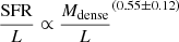$\frac{SFR}{L} \propto {\frac{M_{dense}}{L}}^{(0.55 \pm 0.12)}$ $\frac{\mathrm{SFR}}{L}\propto \frac{M_{\mathrm{dense}}}{L}^{(0.55\pm 0.12)}$ , where M_dense is the mass above the extinction contour of A_V = 7 mag. While the origin of this correlation is elusive, it suggests that there is a link between the (mean) line mass and the specific star formation rate of GMFs. What exactly sets the strength of the relationship is an interesting topic for future study.

In summary, we have performed the first systematic investigation of star-forming content in the Galactic GMFs with a uniform method. Because the SFR surface density and SFE of GMFs are, on average, similar to that of nearby star-forming clouds, our results favor the view that the GMFs are not special objects in the Galaxy. Our method can be also applied to a more general sample of Galactic GMCs to estimate their SFRs. In the near future, a comprehensive investigation of star-forming content toward the Galactic molecular clouds, including GMFs and other GMCs, will be helpful to further assess whether star formation in the GMFs proceeds in a similar manner as in other molecular clouds. Further studies should also be directed to establish if the giant filaments form a class of objects that in some fundamental way differs from other molecular clouds. To do this would require development of a uniform way to define giant filaments; such a definition is currently missing and so hampering the studies of filamentary structures in general.

¹

http://wsa.roe.ac.uk/dr10plus_release.html

²

http://casu.ast.cam.ac.uk/vistasp/

³

http://horus.roe.ac.uk/vsa/

⁴

http://www.stsci.edu/institute/software_hardware/pyraf

⁵

http://iraf.noao.edu/

⁶

http://www.bu.edu/galacticring/

⁷

http://www.astro.ufl.edu/~peterb/research/thrumms/rbank/

⁸

We have excluded the nearby star-forming clouds with Σ_SFR = 0 during the statistics. Thus this value of 0.9 is significantly higher than the value of 0.48 offered in Table 1 of Evans et al. (2014).

Acknowledgments

This project has received funding from the European Union’s Horizon 2020 research and innovation program under grant agreement No. 639459 (PROMISE). This work was supported by the National Natural Science Foundation of China (grants No. 11503086). This work is based in part on observations made with the Spitzer Space Telescope, which is operated by the Jet Propulsion Laboratory, California Institute of Technology under a contract with NASA. This publication makes use of data products from the Wide-field Infrared Survey Explorer, which is a joint project of the University of California, Los Angeles, and the Jet Propulsion Laboratory/California Institute of Technology, funded by the National Aeronautics and Space Administration. This paper made use of information from the Red MSX Source survey database at http://rms.leeds.ac.uk/cgi-bin/public/RMS_DATABASE.cgi which was constructed with support from the Science and Technology Facilities Council of the UK. This publication makes use of molecular line data from the Boston University-FCRAO Galactic Ring Survey (GRS). The GRS is a joint project of Boston University and Five College Radio Astronomy Observatory, funded by the National Science Foundation under grants AST-9800334, AST-0098562, & AST-0100793.

References

Abergel, A., Boulanger, F., Mizuno, A., & Fukui, Y. 1994, ApJ, 423, L59 [NASA ADS] [CrossRef] [Google Scholar]
Abreu-Vicente, J., Ragan, S., Kainulainen, J., et al. 2016, A&A, 590, A131 [NASA ADS] [CrossRef] [EDP Sciences] [Google Scholar]
Alfaro, E. J., & Sánchez, N. 2011, in Computational Star Formation, eds. J. Alves, B. G. Elmegreen, J. M. Girart, & V. Trimble, IAU Symp., 270, 81 [NASA ADS] [Google Scholar]
Alves de Oliveira, C., Schneider, N., Merín, B., et al. 2014, A&A, 568, A98 [NASA ADS] [CrossRef] [EDP Sciences] [Google Scholar]
Anderson, L. D., Bania, T. M., Balser, D. S., & Rood, R. T. 2012, ApJ, 754, 62 [NASA ADS] [CrossRef] [Google Scholar]
André, P., Men’shchikov, A., Bontemps, S., et al. 2010, A&A, 518, L102 [NASA ADS] [CrossRef] [EDP Sciences] [Google Scholar]
André, P., Di Francesco, J., Ward-Thompson, D., et al. 2014, Protostars and Planets VI, 27 [Google Scholar]
Andrews, S. M., Rosenfeld, K. A., Kraus, A. L., & Wilner, D. J. 2013, ApJ, 771, 129 [NASA ADS] [CrossRef] [Google Scholar]
Antoniucci, S., García López, R., Nisini, B., et al. 2014, A&A, 572, A62 [NASA ADS] [CrossRef] [EDP Sciences] [Google Scholar]
Arzoumanian, D., André, P., Didelon, P., et al. 2011, A&A, 529, L6 [Google Scholar]
Bally, J., Langer, W. D., Stark, A. A., & Wilson, R. W. 1987, ApJ, 312, L45 [NASA ADS] [CrossRef] [Google Scholar]
Barnard, E. E., Frost, E. B., & Calvert, M. R. 1927, A Photographic Atlas of Selected Regions of the Milky Way (Washington: Carnegie Institution of Washington) [Google Scholar]
Barnes, P. J., Muller, E., Indermuehle, B., et al. 2015, ApJ, 812, 6 [NASA ADS] [CrossRef] [Google Scholar]
Belloche, A., Schuller, F., Parise, B., et al. 2011, A&A, 527, A145 [NASA ADS] [CrossRef] [EDP Sciences] [Google Scholar]
Benjamin, R. A., Churchwell, E., Babler, B. L., et al. 2003, PASP, 115, 953 [NASA ADS] [CrossRef] [Google Scholar]
Bessell, M. S., & Brett, J. M. 1988, PASP, 100, 1134 [NASA ADS] [CrossRef] [Google Scholar]
Bigiel, F., Leroy, A., Walter, F., et al. 2008, AJ, 136, 2846 [NASA ADS] [CrossRef] [Google Scholar]
Binney, J., & Tremaine, S. 1987, Galactic Dynamics (Princeton: Princeton University Press) [Google Scholar]
Bohlin, R. C., Savage, B. D., & Drake, J. F. 1978, ApJ, 224, 132 [NASA ADS] [CrossRef] [Google Scholar]
Bontemps, S., André, P., Könyves, V., et al. 2010, A&A, 518, L85 [NASA ADS] [CrossRef] [EDP Sciences] [Google Scholar]
Bourke, T. L., Garay, G., Lehtinen, K. K., et al. 1997, ApJ, 476, 781 [NASA ADS] [CrossRef] [Google Scholar]
Butler, M. J., & Tan, J. C. 2012, ApJ, 754, 5 [NASA ADS] [CrossRef] [Google Scholar]
Cambrésy, L. 1999, A&A, 345, 965 [NASA ADS] [Google Scholar]
Caratti o Garatti, A., Garcia Lopez, R., Antoniucci, S., et al. 2012, A&A, 538, A64 [NASA ADS] [CrossRef] [EDP Sciences] [Google Scholar]
Carey, S. J., Noriega-Crespo, A., Mizuno, D. R., et al. 2009, PASP, 121, 76 [NASA ADS] [CrossRef] [Google Scholar]
Casali, M., Adamson, A., Alves de Oliveira, C., et al. 2007, A&A, 467, 777 [NASA ADS] [CrossRef] [EDP Sciences] [Google Scholar]
Chen, H., Myers, P. C., Ladd, E. F., & Wood, D. O. S. 1995, ApJ, 445, 377 [NASA ADS] [CrossRef] [Google Scholar]
Churchwell, E., Babler, B. L., Meade, M. R., et al. 2009, PASP, 121, 213 [NASA ADS] [CrossRef] [Google Scholar]
Comerón, F. 2008, in The Lupus Clouds, ed. B. Reipurth, 295 [Google Scholar]
Cox, N. L. J., Arzoumanian, D., André, P., et al. 2016, A&A, 590, A110 [NASA ADS] [CrossRef] [EDP Sciences] [Google Scholar]
Dalton, G. B., Caldwell, M., Ward, A. K., et al. 2006, in Society of Photo-Optical Instrumentation Engineers (SPIE) Conference Series, Proc. SPIE, 6269, 62690X [Google Scholar]
de Geus, E. J., de Zeeuw, P. T., & Lub, J. 1989, A&A, 216, 44 [NASA ADS] [Google Scholar]
Dickman, R. L. 1978, ApJS, 37, 407 [NASA ADS] [CrossRef] [Google Scholar]
Du, F., & Yang, J. 2008, ApJ, 686, 384 [NASA ADS] [CrossRef] [Google Scholar]
Duarte-Cabral, A., & Dobbs, C. L. 2017, MNRAS, 470, 4261 [NASA ADS] [CrossRef] [Google Scholar]
Dunham, M. M., Crapsi, A., Evans, II., N. J., et al. 2008, ApJS, 179, 249 [NASA ADS] [CrossRef] [Google Scholar]
Dunham, M. M., Stutz, A. M., Allen, L. E., et al. 2014, Protostars and Planets VI, 195 [Google Scholar]
Dunham, M. M., Allen, L. E., Evans, II., N. J., et al. 2015, ApJS, 220, 11 [NASA ADS] [CrossRef] [Google Scholar]
Dzib, S., Loinard, L., Mioduszewski, A. J., et al. 2010, ApJ, 718, 610 [NASA ADS] [CrossRef] [Google Scholar]
Dzib, S., Loinard, L., Mioduszewski, A. J., et al. 2011, Rev. Mex. Astron. Astrofis. Conf. Ser., 40, 231 [NASA ADS] [Google Scholar]
Eden, D. J., Moore, T. J. T., Morgan, L. K., Thompson, M. A., & Urquhart, J. S. 2013, MNRAS, 431, 1587 [NASA ADS] [CrossRef] [Google Scholar]
Elia, D., Molinari, S., Fukui, Y., et al. 2013, ApJ, 772, 45 [NASA ADS] [CrossRef] [Google Scholar]
Emerson, J. P., & Sutherland, W. J. 2010, in Ground-based and Airborne Telescopes III, Proc. SPIE, 7733, 773306 [CrossRef] [Google Scholar]
Enoch, M. L., Young, K. E., Glenn, J., et al. 2006, ApJ, 638, 293 [NASA ADS] [CrossRef] [Google Scholar]
Evans, N. J., Dunham, M. M., Jørgensen, J. K., et al. 2009, ApJS, 181, 321 [NASA ADS] [CrossRef] [Google Scholar]
Evans, II., N. J., Heiderman, A., & Vutisalchavakul, N. 2014, ApJ, 782, 114 [NASA ADS] [CrossRef] [Google Scholar]
Fang, M., Kim, J. S., van Boekel, R., et al. 2013, ApJS, 207, 5 [NASA ADS] [CrossRef] [Google Scholar]
Fernández-López, M., Arce, H. G., Looney, L., et al. 2014, ApJ, 790, L19 [NASA ADS] [CrossRef] [Google Scholar]
Fiege, J. D., & Pudritz, R. E. 2000, MNRAS, 311, 85 [NASA ADS] [CrossRef] [Google Scholar]
Fischera, J., & Martin, P. G. 2012, A&A, 542, A77 [NASA ADS] [CrossRef] [EDP Sciences] [Google Scholar]
Foyle, K., Rix, H.-W., Walter, F., & Leroy, A. K. 2010, ApJ, 725, 534 [NASA ADS] [CrossRef] [Google Scholar]
Franco, G. A. P. 1991, A&A, 251, 581 [NASA ADS] [Google Scholar]
Frerking, M. A., Langer, W. D., & Wilson, R. W. 1982, ApJ, 262, 590 [NASA ADS] [CrossRef] [Google Scholar]
Gaczkowski, B., Preibisch, T., Ratzka, T., et al. 2013, A&A, 549, A67 [NASA ADS] [CrossRef] [EDP Sciences] [Google Scholar]
Gao, Y., & Solomon, P. M. 2004, ApJ, 606, 271 [NASA ADS] [CrossRef] [Google Scholar]
Garden, R. P., Hayashi, M., Hasegawa, T., Gatley, I., & Kaifu, N. 1991, ApJ, 374, 540 [NASA ADS] [CrossRef] [Google Scholar]
Giannini, T., Elia, D., Lorenzetti, D., et al. 2012, A&A, 539, A156 [NASA ADS] [CrossRef] [EDP Sciences] [Google Scholar]
Gomez, M., Hartmann, L., Kenyon, S. J., & Hewett, R. 1993, AJ, 105, 1927 [NASA ADS] [CrossRef] [Google Scholar]
Gong, Y., Mao, R. Q., Fang, M., et al. 2016, A&A, 588, A104 [NASA ADS] [CrossRef] [EDP Sciences] [Google Scholar]
Goodman, A. A., Pineda, J. E., & Schnee, S. L. 2009, ApJ, 692, 91 [NASA ADS] [CrossRef] [Google Scholar]
Goodman, A. A., Alves, J., Beaumont, C. N., et al. 2014, ApJ, 797, 53 [NASA ADS] [CrossRef] [Google Scholar]
Gouliermis, D. A., Hony, S., & Klessen, R. S. 2014, MNRAS, 439, 3775 [NASA ADS] [CrossRef] [Google Scholar]
Greene, T. P., Wilking, B. A., Andre, P., Young, E. T., & Lada, C. J. 1994, ApJ, 434, 614 [NASA ADS] [CrossRef] [Google Scholar]
Griffin, M. J., Abergel, A., Abreu, A., et al. 2010, A&A, 518, L3 [Google Scholar]
Gutermuth, R. A., & Heyer, M. 2015, AJ, 149, 64 [NASA ADS] [CrossRef] [Google Scholar]
Gutermuth, R. A., Myers, P. C., Megeath, S. T., et al. 2008, ApJ, 674, 336 [NASA ADS] [CrossRef] [Google Scholar]
Gutermuth, R. A., Megeath, S. T., Myers, P. C., et al. 2009, ApJS, 184, 18 [NASA ADS] [CrossRef] [Google Scholar]
Hacar, A., Tafalla, M., Kauffmann, J., & Kovács, A. 2013, A&A, 554, A55 [NASA ADS] [CrossRef] [EDP Sciences] [Google Scholar]
Hacar, A., Kainulainen, J., Tafalla, M., Beuther, H., & Alves, J. 2016, A&A, 587, A97 [NASA ADS] [CrossRef] [EDP Sciences] [Google Scholar]
Hambly, N. C., Collins, R. S., Cross, N. J. G., et al. 2008, MNRAS, 384, 637 [NASA ADS] [CrossRef] [Google Scholar]
Harjunpää, P., Lehtinen, K., & Haikala, L. K. 2004, A&A, 421, 1087 [NASA ADS] [CrossRef] [EDP Sciences] [Google Scholar]
Harvey, P. M., Huard, T. L., Jørgensen, J. K., et al. 2008, ApJ, 680, 495 [NASA ADS] [CrossRef] [Google Scholar]
Hatchell, J., Richer, J. S., Fuller, G. A., et al. 2005, A&A, 440, 151 [NASA ADS] [CrossRef] [EDP Sciences] [Google Scholar]
Hatchell, J., Terebey, S., Huard, T., et al. 2012, ApJ, 754, 104 [NASA ADS] [CrossRef] [Google Scholar]
Heiderman, A., & Evans, II., N. J. 2015, ApJ, 806, 231 [NASA ADS] [CrossRef] [Google Scholar]
Heiderman, A., Evans, II., N. J., Allen, L. E., Huard, T., & Heyer, M. 2010, ApJ, 723, 1019 [NASA ADS] [CrossRef] [Google Scholar]
Henning, T., Linz, H., Krause, O., et al. 2010, A&A, 518, L95 [NASA ADS] [CrossRef] [EDP Sciences] [Google Scholar]
Hewett, P. C., Warren, S. J., Leggett, S. K., & Hodgkin, S. T. 2006, MNRAS, 367, 454 [NASA ADS] [CrossRef] [Google Scholar]
Heyer, M., Gutermuth, R., Urquhart, J. S., et al. 2016, A&A, 588, A29 [NASA ADS] [CrossRef] [EDP Sciences] [Google Scholar]
Hill, T., Motte, F., Didelon, P., et al. 2011, A&A, 533, A94 [NASA ADS] [CrossRef] [EDP Sciences] [Google Scholar]
Ho, P. T. P., Moran, J. M., & Rodriguez, L. F. 1982, ApJ, 262, 619 [NASA ADS] [CrossRef] [Google Scholar]
Hodgkin, S. T., Irwin, M. J., Hewett, P. C., & Warren, S. J. 2009, MNRAS, 394, 675 [NASA ADS] [CrossRef] [Google Scholar]
Irwin, M. J. 2008, in 2007 ESO Instrument Calibration Workshop, eds. A. Kaufer, & F. Kerber, 541 [Google Scholar]
Jackson, J. M., Rathborne, J. M., Shah, R. Y., et al. 2006, ApJS, 163, 145 [NASA ADS] [CrossRef] [Google Scholar]
Jackson, J. M., Finn, S. C., Chambers, E. T., Rathborne, J. M., & Simon, R. 2010, ApJ, 719, L185 [NASA ADS] [CrossRef] [Google Scholar]
Jackson, T., Ivezić, Ž., & Knapp, G. R. 2002, MNRAS, 337, 749 [NASA ADS] [CrossRef] [Google Scholar]
Jose, J., Kim, J. S., Herczeg, G. J., et al. 2016, ApJ, 822, 49 [NASA ADS] [CrossRef] [Google Scholar]
Juvela, M., Ristorcelli, I., Pagani, L., et al. 2012, A&A, 541, A12 [NASA ADS] [CrossRef] [EDP Sciences] [Google Scholar]
Kainulainen, J., & Tan, J. C. 2013, A&A, 549, A53 [NASA ADS] [CrossRef] [EDP Sciences] [Google Scholar]
Kainulainen, J., Beuther, H., Henning, T., & Plume, R. 2009, A&A, 508, L35 [NASA ADS] [CrossRef] [EDP Sciences] [Google Scholar]
Kainulainen, J., Ragan, S. E., Henning, T., & Stutz, A. 2013, A&A, 557, A120 [NASA ADS] [CrossRef] [EDP Sciences] [Google Scholar]
Kainulainen, J., Federrath, C., & Henning, T. 2014, Science, 344, 183 [NASA ADS] [CrossRef] [Google Scholar]
Kainulainen, J., Hacar, A., Alves, J., et al. 2016, A&A, 586, A27 [NASA ADS] [CrossRef] [EDP Sciences] [Google Scholar]
Kainulainen, J., Stutz, A. M., Stanke, T., et al. 2017, A&A, 600, A141 [NASA ADS] [CrossRef] [EDP Sciences] [Google Scholar]
Kelly, B. C. 2007, ApJ, 665, 1489 [NASA ADS] [CrossRef] [Google Scholar]
Kennicutt, Jr., R. C. 1998, ApJ, 498, 541 [NASA ADS] [CrossRef] [Google Scholar]
Kim, H.-J., Koo, B.-C., & Davis, C. J. 2015, ApJ, 802, 59 [NASA ADS] [CrossRef] [Google Scholar]
Kirk, J. M., Ward-Thompson, D., Di Francesco, J., et al. 2009, ApJS, 185, 198 [NASA ADS] [CrossRef] [Google Scholar]
Knude, J., & Hog, E. 1998, A&A, 338, 897 [NASA ADS] [Google Scholar]
Koenig, X. P., & Leisawitz, D. T. 2014, ApJ, 791, 131 [NASA ADS] [CrossRef] [Google Scholar]
Koenig, X. P., Leisawitz, D. T., Benford, D. J., et al. 2012, ApJ, 744, 130 [NASA ADS] [CrossRef] [Google Scholar]
Könyves, V., André, P., Men’shchikov, A., et al. 2010, A&A, 518, L106 [NASA ADS] [CrossRef] [EDP Sciences] [Google Scholar]
Könyves, V., André, P., Men’shchikov, A., et al. 2015, A&A, 584, A91 [NASA ADS] [CrossRef] [EDP Sciences] [Google Scholar]
Kraus, A. L., & Hillenbrand, L. A. 2008, ApJ, 686, L111 [NASA ADS] [CrossRef] [Google Scholar]
Kroupa, P. 2001, MNRAS, 322, 231 [NASA ADS] [CrossRef] [Google Scholar]
Krumholz, M. R., Dekel, A., & McKee, C. F. 2012, ApJ, 745, 69 [NASA ADS] [CrossRef] [Google Scholar]
Kryukova, E., Megeath, S. T., Gutermuth, R. A., et al. 2012, AJ, 144, 31 [NASA ADS] [CrossRef] [Google Scholar]
Kryukova, E., Megeath, S. T., Hora, J. L., et al. 2014, AJ, 148, 11 [NASA ADS] [CrossRef] [Google Scholar]
Lada, C. J. 1987, in Star Forming Regions, eds. M. Peimbert, & J. Jugaku, IAU Symp., 115, 1 [NASA ADS] [CrossRef] [Google Scholar]
Lada, C. J., & Wilking, B. A. 1984, ApJ, 287, 610 [NASA ADS] [CrossRef] [Google Scholar]
Lada, C. J., Lada, E. A., Clemens, D. P., & Bally, J. 1994, ApJ, 429, 694 [NASA ADS] [CrossRef] [Google Scholar]
Lada, C. J., Lombardi, M., & Alves, J. F. 2009, ApJ, 703, 52 [NASA ADS] [CrossRef] [Google Scholar]
Lada, C. J., Lombardi, M., & Alves, J. F. 2010, ApJ, 724, 687 [NASA ADS] [CrossRef] [Google Scholar]
Lada, C. J., Forbrich, J., Lombardi, M., & Alves, J. F. 2012, ApJ, 745, 190 [NASA ADS] [CrossRef] [Google Scholar]
Lada, C. J., Lombardi, M., Roman-Zuniga, C., Forbrich, J., & Alves, J. F. 2013, ApJ, 778, 133 [NASA ADS] [CrossRef] [Google Scholar]
Lada, C. J., Lewis, J. A., Lombardi, M., & Alves, J. 2017, A&A, 606, A100 [NASA ADS] [CrossRef] [EDP Sciences] [Google Scholar]
Landy, S. D., & Szalay, A. S. 1993, ApJ, 412, 64 [NASA ADS] [CrossRef] [Google Scholar]
Larson, R. B. 1981, MNRAS, 194, 809 [NASA ADS] [CrossRef] [Google Scholar]
Larson, R. B. 1995, MNRAS, 272, 213 [NASA ADS] [Google Scholar]
Lawrence, A., Warren, S. J., Almaini, O., et al. 2007, MNRAS, 379, 1599 [NASA ADS] [CrossRef] [MathSciNet] [Google Scholar]
Lee, K. I., Fernández-López, M., Storm, S., et al. 2014, ApJ, 797, 76 [NASA ADS] [CrossRef] [Google Scholar]
Lee, E. J., Miville-Deschênes, M.-A., & Murray, N. W. 2016, ApJ, 833, 229 [NASA ADS] [CrossRef] [Google Scholar]
Levshakov, S. A., Reimers, D., & Henkel, C. 2016, A&A, 586, A126 [NASA ADS] [CrossRef] [EDP Sciences] [Google Scholar]
Lewis, J. R., Irwin, M., & Bunclark, P. 2010, in Astronomical Data Analysis Software and Systems XIX, eds. Y. Mizumoto, K. I. Morita, & M. Ohishi, ASP Conf. Ser., 434, 91 [NASA ADS] [Google Scholar]
Li, G.-X., Wyrowski, F., Menten, K., & Belloche, A. 2013, A&A, 559, A34 [NASA ADS] [CrossRef] [EDP Sciences] [Google Scholar]
Li, G.-X., Urquhart, J. S., Leurini, S., et al. 2016, A&A, 591, A5 [NASA ADS] [CrossRef] [EDP Sciences] [Google Scholar]
Lombardi, M. 2009, A&A, 493, 735 [NASA ADS] [CrossRef] [EDP Sciences] [Google Scholar]
Lombardi, M., & Alves, J. 2001, A&A, 377, 1023 [NASA ADS] [CrossRef] [EDP Sciences] [Google Scholar]
Lucas, P. W., Hoare, M. G., Longmore, A., et al. 2008, MNRAS, 391, 136 [NASA ADS] [CrossRef] [Google Scholar]
Lumsden, S. L., Hoare, M. G., Urquhart, J. S., et al. 2013, ApJS, 208, 11 [NASA ADS] [CrossRef] [Google Scholar]
Lynds, B. T. 1962, ApJS, 7, 1 [NASA ADS] [CrossRef] [Google Scholar]
Mallick, K. K., Kumar, M. S. N., Ojha, D. K., et al. 2013, ApJ, 779, 113 [NASA ADS] [CrossRef] [Google Scholar]
Marshall, D. J., Robin, A. C., Reylé, C., Schultheis, M., & Picaud, S. 2006, A&A, 453, 635 [NASA ADS] [CrossRef] [EDP Sciences] [Google Scholar]
Mattern, M., Kainulainen, J., Zhang, M., & Beuther, H. 2018, A&A, 616, A78 [NASA ADS] [CrossRef] [EDP Sciences] [Google Scholar]
Meingast, S., Lombardi, M., & Alves, J. 2017, A&A, 601, A137 [NASA ADS] [CrossRef] [EDP Sciences] [Google Scholar]
Men’shchikov, A., André, P., Didelon, P., et al. 2010, A&A, 518, L103 [NASA ADS] [CrossRef] [EDP Sciences] [Google Scholar]
Meyer, M. R., Calvet, N., & Hillenbrand, L. A. 1997, AJ, 114, 288 [NASA ADS] [CrossRef] [Google Scholar]
Minniti, D., Lucas, P. W., Emerson, J. P., et al. 2010, New Astron., 15, 433 [NASA ADS] [CrossRef] [Google Scholar]
Miville-Deschênes, M.-A., Murray, N., & Lee, E. J. 2017, ApJ, 834, 57 [NASA ADS] [CrossRef] [Google Scholar]
Molinari, S., Swinyard, B., Bally, J., et al. 2010, PASP, 122, 314 [NASA ADS] [CrossRef] [Google Scholar]
Molinari, S., Bally, J., Glover, S., et al. 2014, Protostars and Planets VI, 125 [Google Scholar]
Molinari, S., Schisano, E., Elia, D., et al. 2016, A&A, 591, A149 [NASA ADS] [CrossRef] [EDP Sciences] [Google Scholar]
Morales, E. F. E., & Robitaille, T. P. 2017, A&A, 598, A136 [NASA ADS] [CrossRef] [EDP Sciences] [Google Scholar]
Myers, P. C. 2009, ApJ, 700, 1609 [NASA ADS] [CrossRef] [EDP Sciences] [Google Scholar]
Myers, P. C., & Ladd, E. F. 1993, ApJ, 413, L47 [NASA ADS] [CrossRef] [Google Scholar]
Nakajima, Y., Tachihara, K., Hanawa, T., & Nakano, M. 1998, ApJ, 497, 721 [NASA ADS] [CrossRef] [Google Scholar]
Neuhäuser, R., & Forbrich, J. 2008, in The Corona Australis Star Forming Region, ed. B. Reipurth, 735 [Google Scholar]
Oliveira, I., Merín, B., Pontoppidan, K. M., et al. 2009, ApJ, 691, 672 [NASA ADS] [CrossRef] [Google Scholar]
Ostriker, J. 1964, ApJ, 140, 1056 [NASA ADS] [CrossRef] [MathSciNet] [Google Scholar]
Palmeirim, P., André, P., Kirk, J., et al. 2013, A&A, 550, A38 [NASA ADS] [CrossRef] [EDP Sciences] [Google Scholar]
Perault, M., Omont, A., Simon, G., et al. 1996, A&A, 315, L165 [NASA ADS] [Google Scholar]
Peretto, N., & Fuller, G. A. 2009, A&A, 505, 405 [NASA ADS] [CrossRef] [EDP Sciences] [Google Scholar]
Pineda, J. E., Caselli, P., & Goodman, A. A. 2008, ApJ, 679, 481 [NASA ADS] [CrossRef] [Google Scholar]
Pineda, J. L., Goldsmith, P. F., Chapman, N., et al. 2010, ApJ, 721, 686 [NASA ADS] [CrossRef] [Google Scholar]
Planck Collaboration Int. XXXII. 2016, A&A, 586, A135 [NASA ADS] [CrossRef] [EDP Sciences] [Google Scholar]
Planck Collaboration Int. XXXIII. 2016, A&A, 586, A136 [NASA ADS] [CrossRef] [EDP Sciences] [Google Scholar]
Poglitsch, A., Waelkens, C., Geis, N., et al. 2010, A&A, 518, L2 [NASA ADS] [CrossRef] [EDP Sciences] [Google Scholar]
Ragan, S. E., Henning, T., Tackenberg, J., et al. 2014, A&A, 568, A73 [NASA ADS] [CrossRef] [EDP Sciences] [Google Scholar]
Ragan, S. E., Moore, T. J. T., Eden, D. J., et al. 2016, MNRAS, 462, 3123 [NASA ADS] [CrossRef] [Google Scholar]
Ramón-Fox, F. G., & Bonnell, I. A. 2018, MNRAS, 474, 2028 [NASA ADS] [CrossRef] [Google Scholar]
Rapson, V. A., Pipher, J. L., Gutermuth, R. A., et al. 2014, ApJ, 794, 124 [NASA ADS] [CrossRef] [EDP Sciences] [Google Scholar]
Recchi, S., Hacar, A., & Palestini, A. 2014, MNRAS, 444, 1775 [NASA ADS] [CrossRef] [Google Scholar]
Reid, M. J., Menten, K. M., Brunthaler, A., et al. 2014, ApJ, 783, 130 [Google Scholar]
Ripple, F., Heyer, M. H., Gutermuth, R., Snell, R. L., & Brunt, C. M. 2013, MNRAS, 431, 1296 [NASA ADS] [CrossRef] [Google Scholar]
Robin, A. C., Reylé, C., Derrière, S., & Picaud, S. 2003, A&A, 409, 523 [NASA ADS] [CrossRef] [EDP Sciences] [Google Scholar]
Robitaille, T. P., Whitney, B. A., Indebetouw, R., Wood, K., & Denzmore, P. 2006, ApJS, 167, 256 [NASA ADS] [CrossRef] [Google Scholar]
Robitaille, T. P., Meade, M. R., Babler, B. L., et al. 2008, AJ, 136, 2413 [NASA ADS] [CrossRef] [Google Scholar]
Roccatagliata, V., Dale, J. E., Ratzka, T., et al. 2015, A&A, 584, A119 [NASA ADS] [CrossRef] [EDP Sciences] [Google Scholar]
Rohlfs, K., & Wilson, T. L. 2004, Tools of Radio Astronomy (Berlin: Springer) [CrossRef] [Google Scholar]
Roman-Duval, J., Jackson, J. M., Heyer, M., et al. 2009, ApJ, 699, 1153 [NASA ADS] [CrossRef] [Google Scholar]
Romero, G. A., Schreiber, M. R., Cieza, L. A., et al. 2012, ApJ, 749, 79 [NASA ADS] [CrossRef] [Google Scholar]
Rygl, K. L. J., Benedettini, M., Schisano, E., et al. 2013, A&A, 549, L1 [NASA ADS] [CrossRef] [EDP Sciences] [Google Scholar]
Sadavoy, S. I. 2013, PhD Thesis, University of Victoria, Canada [Google Scholar]
Saito, R. K., Hempel, M., Minniti, D., et al. 2012, A&A, 537, A107 [NASA ADS] [CrossRef] [EDP Sciences] [Google Scholar]
Samal, M. R., Ojha, D. K., Jose, J., et al. 2015, A&A, 581, A5 [NASA ADS] [CrossRef] [EDP Sciences] [Google Scholar]
Saral, G., Hora, J. L., Willis, S. E., et al. 2015, ApJ, 813, 25 [NASA ADS] [CrossRef] [Google Scholar]
Schmalzl, M., Kainulainen, J., Quanz, S. P., et al. 2010, ApJ, 725, 1327 [NASA ADS] [CrossRef] [Google Scholar]
Schneider, S., & Elmegreen, B. G. 1979, ApJS, 41, 87 [NASA ADS] [CrossRef] [Google Scholar]
Schuller, F., Menten, K. M., Contreras, Y., et al. 2009, A&A, 504, 415 [NASA ADS] [CrossRef] [EDP Sciences] [Google Scholar]
Seigar, M. S., & James, P. A. 2002, MNRAS, 337, 1113 [NASA ADS] [CrossRef] [Google Scholar]
Shimajiri, Y., André, P., Braine, J., et al. 2017, A&A, 604, A74 [NASA ADS] [CrossRef] [EDP Sciences] [Google Scholar]
Siess, L., Dufour, E., & Forestini, M. 2000, A&A, 358, 593 [Google Scholar]
Silva-Villa, E., & Larsen, S. S. 2012, A&A, 537, A145 [NASA ADS] [CrossRef] [EDP Sciences] [Google Scholar]
Simon, M. 1997, ApJ, 482, L81 [NASA ADS] [CrossRef] [Google Scholar]
Simon, R., Rathborne, J. M., Shah, R. Y., Jackson, J. M., & Chambers, E. T. 2006, ApJ, 653, 1325 [NASA ADS] [CrossRef] [Google Scholar]
Skrutskie, M. F., Cutri, R. M., Stiening, R., et al. 2006, AJ, 131, 1163 [NASA ADS] [CrossRef] [Google Scholar]
Solomon, P. M., & Sage, L. J. 1988, ApJ, 334, 613 [NASA ADS] [CrossRef] [Google Scholar]
Solomon, P. M., Rivolo, A. R., Barrett, J., & Yahil, A. 1987, ApJ, 319, 730 [NASA ADS] [CrossRef] [Google Scholar]
Soto, M., Barbá, R., Gunthardt, G., et al. 2013, A&A, 552, A101 [NASA ADS] [CrossRef] [EDP Sciences] [Google Scholar]
Sousbie, T. 2011, MNRAS, 414, 350 [NASA ADS] [CrossRef] [Google Scholar]
Spitzer Science Center 2009, VizieR Online Data Catalog: II/293 [Google Scholar]
Stetson, P. B. 1987, PASP, 99, 191 [NASA ADS] [CrossRef] [Google Scholar]
Stodólkiewicz, J. S. 1963, Acta Astron., 13, 30 [NASA ADS] [Google Scholar]
Storm, S., Mundy, L. G., Fernández-López, M., et al. 2014, ApJ, 794, 165 [NASA ADS] [CrossRef] [Google Scholar]
Straižys, V., Černis, K., & BartaŠiūtė, S. 2003, A&A, 405, 585 [NASA ADS] [CrossRef] [EDP Sciences] [Google Scholar]
Stutz, A. M., & Gould, A. 2016, A&A, 590, A2 [NASA ADS] [CrossRef] [EDP Sciences] [Google Scholar]
Stutz, A. M., & Kainulainen, J. 2015, A&A, 577, L6 [NASA ADS] [CrossRef] [EDP Sciences] [Google Scholar]
Taylor, M. B. 2006, in Astronomical Data Analysis Software and Systems XV, eds. C. Gabriel, C. Arviset, D. Ponz, & S. Enrique, ASP Conf. Ser., 351, 666 [NASA ADS] [Google Scholar]
Toalá, J. A., Vázquez-Semadeni, E., & Gómez, G. C. 2012, ApJ, 744, 190 [NASA ADS] [CrossRef] [Google Scholar]
Traficante, A., Calzoletti, L., Veneziani, M., et al. 2011, MNRAS, 416, 2932 [NASA ADS] [CrossRef] [Google Scholar]
Vallée, J. P. 2008, AJ, 135, 1301 [NASA ADS] [CrossRef] [Google Scholar]
Vallée, J. P. 2017, Astron. Rev., 13, 113 [Google Scholar]
van Kempen, T. A., van Dishoeck, E. F., Salter, D. M., et al. 2009, A&A, 498, 167 [NASA ADS] [CrossRef] [EDP Sciences] [Google Scholar]
Veneziani, M., Elia, D., Noriega-Crespo, A., et al. 2013, A&A, 549, A130 [NASA ADS] [CrossRef] [EDP Sciences] [Google Scholar]
Vutisalchavakul, N., Evans, II., N. J., & Heyer, M. 2016, ApJ, 831, 73 [NASA ADS] [CrossRef] [EDP Sciences] [Google Scholar]
Wall, W. F., Puerari, I., Tilanus, R., et al. 2016, MNRAS, 459, 1440 [NASA ADS] [CrossRef] [Google Scholar]
Wang, K., Testi, L., Ginsburg, A., et al. 2015, MNRAS, 450, 4043 [NASA ADS] [CrossRef] [MathSciNet] [Google Scholar]
Wang, K., Testi, L., Burkert, A., et al. 2016, ApJS, 226, 9 [NASA ADS] [CrossRef] [Google Scholar]
Warren, S. J., Cross, N. J. G., Dye, S., et al. 2007, ArXiv e-prints [arXiv:astro-ph/0703037] [Google Scholar]
Whittet, D. C. B., Prusti, T., Franco, G. A. P., et al. 1997, A&A, 327, 1194 [NASA ADS] [Google Scholar]
Wilking, B. A., Gagné, M., & Allen, L. E. 2008, in Star Formation in the ρ Ophiuchi Molecular Cloud, ed. B. Reipurth, 351 [Google Scholar]
Willis, S., Marengo, M., Allen, L., et al. 2013, ApJ, 778, 96 [NASA ADS] [CrossRef] [Google Scholar]
Wilson, T. L., & Rood, R. 1994, ARA&A, 32, 191 [NASA ADS] [CrossRef] [Google Scholar]
Wright, E. L., Eisenhardt, P. R. M., Mainzer, A. K., et al. 2010, AJ, 140, 1868 [NASA ADS] [CrossRef] [Google Scholar]
Wu, Y., Wei, Y., Zhao, M., et al. 2004, A&A, 426, 503 [NASA ADS] [CrossRef] [EDP Sciences] [Google Scholar]
Wu, J., Evans, II., N. J., Gao, Y., et al. 2005, ApJ, 635, L173 [NASA ADS] [CrossRef] [Google Scholar]
Xiong, F., Chen, X., Yang, J., et al. 2017, ApJ, 838, 49 [NASA ADS] [CrossRef] [Google Scholar]
Xu, Y., Li, J. J., Reid, M. J., et al. 2013, ApJ, 769, 15 [NASA ADS] [CrossRef] [Google Scholar]
Xue, M., Jiang, B. W., Gao, J., et al. 2016, ApJS, 224, 23 [NASA ADS] [CrossRef] [Google Scholar]
Zhang, M., Fang, M., Wang, H., et al. 2015, ApJS, 219, 21 [NASA ADS] [CrossRef] [Google Scholar]
Zucker, C., Battersby, C., & Goodman, A. 2015, ApJ, 815, 23 [NASA ADS] [CrossRef] [Google Scholar]
Zucker, C., Battersby, C., & Goodman, A. 2018, ApJ, 864, 153 [NASA ADS] [CrossRef] [Google Scholar]

Appendix A: Obtaining column density maps of GMFs

Ragan et al. (2014), Wang et al. (2015), and Abreu-Vicente et al. (2016) use the GRS and ThrUMMS data to investigate the velocity structure of their samples and present the radial velocity range for each giant filament. Thus for the GMFs from Ragan et al. (2014), Wang et al. (2015), and Abreu-Vicente et al. (2016), we adopted the velocity ranges offered by the corresponding papers. Zucker et al. (2015) also use the GRS and ThrUMMS data to identify the velocity coherent filaments. However, they offer only the radial central velocities for their samples. Li et al. (2016) and Wang et al. (2016) used several different gas tracers such as NH₃ and HCO⁺ to investigate the velocity structures of their samples. Therefore, for the GMFs from Zucker et al. (2015), Li et al. (2016), and Wang et al. (2016), we re-checked them in the ¹³CO data cubes and obtained the radial velocity ranges.

Figure A.1 shows this process of an example, GMF 20 (i.e., BC_026.94−0.30) identified originally by Zucker et al. (2015): firstly, we obtain its ¹³CO average spectrum (black line); secondly, we use the multiple Gaussian functions to fit the average spectrum (red line) and then obtain the positions and FWHMs for most of strong velocity components; thirdly, the closest velocity component to the central velocity offered by the corresponding paper is adopted as the velocity range for this object. During this process, we found that three GMFs identified by Li et al. (2016) or Wang et al. (2016) show the indication of self-absorption in ¹³CO lines. Thus we excluded these three filaments from our samples.

Based on the velocity range of each GMF, we collapsed the data cube to obtain the ¹³CO intensity map and velocity dispersion map. Due to the lack of ¹²CO data in GRS survey and different coverage of ¹²CO and ¹³CO data in ThrUMMS survey, we do not try to obtain the excitation temperature maps based on ¹²CO data. Alternatively, we simply adopted a value of 10 K as the excitation temperature (T_ex) for all GMFs.

The ¹³CO column density can be obtained via (Ho et al. 1982; Garden et al. 1991; Bourke et al. 1997):

$\begin{matrix} N (^{13} CO) = 2.42 \times 10^{14} \frac{1 + 0.88 / T_{ex}}{1 - e^{- 5.29 / T_{ex}}} \int T_{mb}^{*} (^{13} CO) d v, \end{matrix}$ $\begin{aligned} N(^{13} {\text{ CO}})=2.42 \times 10^{14}\frac{1+0.88/T_{\text{ ex}}}{1-\mathrm{e}^{-5.29/T_{\text{ ex}}}}\int T_{\text{ mb}}^{*}(^{13}{\text{ CO}}) {\text{ d}}{ v}, \end{aligned}$ (A.1)

where $T_{mb}^{*} (^{13} CO)$ $T_{\mathrm{mb}}^{*}(^{13}{\mathrm{CO}})$ is the main-beam temperature in ¹³CO emission and v is the line velocity. We adopt the ¹²C/¹³C ratio of 77 (Wilson & Rood 1994) and N(H₂)/N(¹²CO) = 1.1 × 10⁴ (Frerking et al. 1982) to convert N(¹³CO) to the molecular hydrogen column density. And then we convert N(H₂) to the visual extinction units with the relation of N(H₂) (cm⁻²) = 0.94 × 10²¹A_V (mag) (Bohlin et al. 1978).

We note that some GMFs were identified several times by different papers. Excluding the redundant GMFs and four GMFs that are not fully covered by ¹³CO data, we can obtain the column density maps for 56 GMFs.

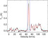Fig. A.1.

¹³CO average spectrum of GMF 20 (i.e., BC_026.94−0.30) that is identified originally by Zucker et al. (2015). The red curve shows the best fitting using the multiple Gaussian components. The dashed line marks the central velocity offered by Zucker et al. (2015) and the blue solid lines show the velocity range of this component.

Nessie is a special case. The sensitivity of the ThrUMMS data in the region with Nessie is not enough to trace the main filamentary part of Nessie. Thus we decided to use the extinction map that is constructed with the technique improved by Kainulainen & Tan (2013) for Nessie. This extinction mapping technique is based on combining extinction maps made at two wavelength regimes: in near-infrared using NICER (Near-Infrared Color Excess Revisited, Lombardi & Alves 2001) and in mid-infrared using the absorption against the Galactic background (Peretto & Fuller 2009; Butler & Tan 2012). Using this method, we obtain a high resolution (∼2″) extinction map of the Nessie. The details about the high-resolution extinction map of Nessie can be found in Mattern et al. (2018).

Appendix B: Measuring physical parameters of GMFs

All the pixels of the column density map inside the GMF boundary are fitted with an ellipse as shown in Figs. 3–9 of the main text. The coordinates and length of each GMF are defined as the center and major axis of the ellipse, respectively. The area of each GMF is the area of pixels inside the boundary (A_V = 3 mag) of the column density map. The distance of each GMF is adopted from the corresponding reference paper that is given in the last column of Table H.1. The Galactocentric radius (R_gal) and the height above the Galactic midplane (z) are calculated based on the coordinates and distances of the GMFs.

We also obtain the ¹³CO line width distribution map (the second moment map) for each GMF. Figure B.1 shows an example of GMF 39 (CFG047.06+0.26). The mean line width (Δv) of a GMF is defined as the average value of the line widths inside the GMF boundary.

We integrated the column density maps of the GMFs down to A_V = 3 mag and A_V = 7 mag to obtain the total mass of the cloud (M_cloud) and the mass of dense gas (M_dense). The average gas surface densities (Σ_gas) and the cloud mass per unit length ( $\frac{M_{cloud}}{L}$ $\frac{M_{\mathrm{cloud}}}{L}$ ) can be also obtained with M_cloud, areas and lengths of the GMFs.

Assuming the spherical morphology, the free-fall time of a GMF can be estimated with the formula (Binney & Tremaine 1987; Krumholz et al. 2012)

$\begin{matrix} t_{ff,s} = \sqrt{\frac{3 π}{32 G ρ}}, \end{matrix}$ $\begin{aligned} t_{\text{ ff,s}} = \sqrt{\frac{3\pi }{32G\rho }}, \end{aligned}$ (B.1)

where ρ is the average volume density. We note that we have used an additional subscript “s” in t_ff, s to emphasize that this free-fall time is estimated based on the spherical morphology assumption.

Of course, the assumption of spherical morphology is not reasonable for the filamentary structures, especially the filaments with large aspect ratio of length to radius. Toalá et al. (2012) computed the free-fall time for finite, uniform, and self-gravitating filamentary clouds and suggested that the free-fall time of a filament whose volume density remains constant during the collapse can be obtained with the formula

$\begin{matrix} t_{ff,f} = \frac{2}{π} \sqrt{\frac{8 A}{3}} t_{ff,s}', \end{matrix}$ $\begin{aligned} t_{\text{ ff,f}} = \frac{2}{\pi }\sqrt{\frac{8A}{3}}t_{\text{ ff,s}}{\prime }, \end{aligned}$ (B.2)

where A is the aspect ratio of the filament and t_ff, s′ is the free-fall time of an spherical cloud with the same volume density as the filamentary cloud. We note that here we also added an subscript “f” in t_ff, f to emphasize that this free-fall time is obtained based on the filamentary morphology assumption. Here we also note as a caveat that we could still underestimate the free-fall time because we could significantly underestimate the aspect ratio of GMFs (see Sect. 4.1).

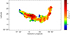Fig. B.1.

¹³CO line width distribution map (obtained from the moment 2 map) of GMF 39 (CFG047.06+0.26).

Appendix C: Method used for YSO identification

There are six steps in the process of YSO identification. The method is mainly based on the YSO classification schemes presented by Gutermuth et al. (2009) and Koenig & Leisawitz (2014). We also combined several color criteria from Robitaille et al. (2008), Veneziani et al. (2013), and Saral et al. (2015) to isolate the AGB stars.

Step 1: we used the method suggested by Gutermuth et al. (2008, 2009) to identify YSOs. The details about this multiphase source classification scheme can be found in the appendix of Gutermuth et al. (2009). Here we only summarize our process (also see the description in Rapson et al. 2014 and Zhang et al. 2015).

There are three phases in the YSO selection scheme suggested by Gutermuth et al. (2009). Phase 1 is applied to the sources that are detected in all four IRAC bands with photometric uncertainties of <0.2 mag. After removing the contaminants of star-forming galaxies, broad-line active galactic nuclei (AGNs), unresolved knots of shock emission, and sources that have polycyclic aromatic hydrocarbon-contaminated apertures, the sources with infrared excess are identified as Class I and Class II sources (see Fig. C.1). The remaining sources are classified as Class III/field sources.

Phase 2 is applied to the sources that lack detections at either 5.8 or 8.0 μm, but have high-quality (σ < 0.05 mag) near-infrared detections in J, H, and K_s bands. We also require the detections at 3.6 and 4.5 μm with the uncertainties of σ < 0.13 mag in order to minimize the contamination of field stars in the crowded regions. To distinguish the sources with IR excess from those that are simply reddened by dust along the line of sight, we deredden the photometry of sources based on the extinction law presented in Xue et al. (2016). The dereddened Ks–[3.6] and [3.6]–[4.5] colors are used to identify the sources with infrared excess at 3.6 and 4.5 μm, accounting for photometric uncertainty (see panel a of Fig. C.2). Sources with no IR excess at 3.6 and 4.5 μm are presumed as Class III/field sources.

Phase 3 is applied to the sources that have detections in the MIPS 24 μm band with the photometric uncertainties of <0.2 mag. The Class III/field sources that were classified in the previous two phases are re-examined, and the transition disks are isolated. The sources that lack detections in some IRAC bands, but are very bright at 24 μm are classified as deeply embedded Class I protostars (see panels b and c of Fig. C.2). The AGNs and shock-emission-dominated sources that were classified as contaminants in phase 1 are also re-examined and identified as Class I sources if they have bright MIPS 24 μm photometry. Finally, the Class I sources that were classified in all three phases are re-analyzed to ensure their nature. Figures C.1 and C.2 show the multicolor criteria mentioned above that are used to identify YSOs in GMF 39 (CFG047.06+0.26).

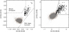Fig. C.1.

Color–color diagrams used for identification of Class I (left), and Class II (right) sources in phase 1 of the classification scheme presented by Gutermuth et al. (2009) for an example of GMF 39 (CFG047.06+0.26). The black filled circles represent the selected Class I and Class II sources. The remaining Class III/field sources are indicated by the gray dots. The black lines show the color criteria of the classification scheme.

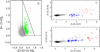Fig. C.2.

Color–color diagrams used for YSO identification in phase 2 (panel a) and phase 3 (panels b and c) classification schemes suggested by Gutermuth et al. (2009) for an example of GMF 39 (CFG047.06+0.26). The Class I sources identified in phase 2 and the protostars identified in phase 3 are marked with red dots. The Class II sources isolated in phase 2 are labeled with green dots while the transition disks classified in phase 3 are shown with blue dots.

Step 2: the 70 μm photometry of the Herschel Hi-Gal catalog (Molinari et al. 2016) is used to identify the protostellar objects. Due to the variation of background in the Galactic plane, Molinari et al. (2016) find that there is no good parameter that can be uniquely taken as a measure of the reliability of a source detection and they suggested to use cross-matching sources in different bands to eliminate the spurious detections. On the other hand, van Kempen et al. (2009) and Heiderman & Evans (2015) suggested that the detection of dense gas around a protostar candidate was a good indicator of a bona fide protostar. Therefore, in the present work only the compact sources with the detections at [70, 160, 250, 350] μm or [70, 250, 350, 500] μm, simultaneously, are identified as the protostars, which means that these protostars have the counterparts of dense cores and thus have high probabilities to be the bona fide protostars. We also crossmatched the protostars identified in this step with the YSOs identified in Step 1 and only keep the additional protostars in our final YSO catalog.

Step 3: all the YSOs identified in the previous steps are re-examined to isolate the possible AGB stars. We combined several classification criteria from Robitaille et al. (2008), Veneziani et al. (2013), and Saral et al. (2015). The YSOs are classified as AGBs if they follow any of the following criteria, as shown in Fig. C.3:

$\begin{matrix} 3 < [3.6] < 9.5 and 0.2 < [3.6] - [4.5] < 1.25, \end{matrix}$ $\begin{aligned} 3 < [3.6] < 9.5\,\mathrm{and}\,0.2 < [3.6]{-}[4.5] < 1.25, \end{aligned}$

or

$\begin{matrix} 3.5 < [3.6] < 9.5 and 0.4 < [3.6] - [8.0] < 2.6, \end{matrix}$ $\begin{aligned} 3.5 < [3.6] < 9.5\,\mathrm{and}\,0.4 < [3.6]{-}[8.0] < 2.6, \end{aligned}$

or

$\begin{matrix} [4.5] > 7.8 and [8.0] - [24] < 2.5, \end{matrix}$ $\begin{aligned}[4.5] > 7.8\,\mathrm{and}\,[8.0]{-}[24] < 2.5, \end{aligned}$

or

$\begin{matrix} 0.2 < \frac{log (\frac{S_{[70]}}{S_{[160]}})}{log (\frac{S_{[70]}}{S_{[250]}})} < 0.9 and 1.2 < \frac{log (\frac{S_{[70]}}{S_{[350]}})}{log (\frac{S_{[160]}}{S_{[350]}})} < 3.3, \end{matrix}$ $\begin{aligned} 0.2 < \frac{{\text{ log}}(\frac{S_{[70]}}{S_{[160]}})}{{\text{ log}}(\frac{S_{[70]}}{S_{[250]}})} < 0.9\,\mathrm{and}\,1.2 < \frac{{\text{ log}} (\frac{S_{[70]}}{S_{[350]}})}{{\text{ log}}(\frac{S_{[160]}}{S_{[350]}})} < 3.3, \end{aligned}$

where S_[x] is the flux at [X] band.

Step 4: we used the selection scheme suggested by Koenig & Leisawitz (2014) to identify bright YSOs that are saturated on Spitzer images based on the AllWISE+NIR catalog. Koenig & Leisawitz (2014) found that the fake source contamination in the Galactic plane can be up to 30% in the W1 band and even 97% in the W4 band. Thus they firstly used the signal-to-noise and reduced chi-squared parameters given in the AllWISE photometric catalog to eliminate the spurious detections, which can suppress the contamination rate in any band down to <7%.

YSO identification and classification scheme resembles the one described in Koenig et al. (2012) and the details can be found in Koenig & Leisawitz (2014). Here we also give a short description of this process.

Firstly, the contaminations of star-forming galaxies and AGNs are filtered out based on their photometry in W1, W2, and W3 bands. Then the Class I and Class II sources are identified using their colors in W1, W2, and W3 bands (see the top left panel of Fig. C.4). Secondly, the remaining sources with the H and K_s detections are identified as YSOs using the color criteria shown in the top right panel of Fig. C.4. Thirdly, the W4 (22 μm) photometry is used to identify transition disks and to retrieve possible protostars from the AGN candidates with the color criteria shown in the bottom panels of Fig. C.4. Finally, all YSOs identified in this step are re-examined to exclude the possible AGB stars and CBe stars (see Fig. C.5). We crossmatched the YSOs identified in this step with the YSOs identified in the previous steps and only the additional YSOs identified in this step are kept in our final YSO catalog.

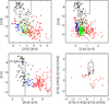Fig. C.3.

Color criteria used to isolate the possible AGB stars from the YSOs in Step 3 for an example of GMF 39 (CFG047.06+0.26). The red dots indicate the Class I sources or protostars while the green and blue dots label the Class II and transition disks, respectively. The AGBs are marked with black dots. The black solid lines show the boundaries of the classification criteria.

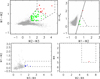Fig. C.4.

Color–color diagrams and the color-magnitude diagram used in Step 4 for a example of GMF 39 (CFG047.06+0.26). The red dots indicate the Class I sources and protostars identified in the YSO classification scheme suggested by Koenig & Leisawitz (2014) while the green and blue dots label the Class II sources and transition disks, respectively.

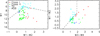Fig. C.5.

Color-magnitude and color–color diagrams used to isolate the possible AGBs from YSOs in Step 4 for an example of GMF 39 (CFG047.06+0.26).

Step 5: all the YSOs identified in the above steps are re-examined in the JHK_s color–color diagram as shown in Fig. 10 of the main text. The sources located in region 1 are classified as possible giants (e.g., AGB stars). We note that we only plot the YSOs after excluding the giants in Fig. 10. Because we account the photometric uncertainties of sources, there are still several YSOs locating in region 1 of Fig 10.

Step 6: the sources classified as “YSO”, “HII regions” or “HII/YSO” in the RMS catalog (Lumsden et al. 2013) are selected as MYSOs and matched with the YSOs identified in the above steps. We kept the additional MYSOs in our final YSO catalog.

Appendix D: Estimating uncertainties of the GMF parameters with the Monte Carlo method

D.1. Uncertainty of SFR

Assuming that the mass completeness ( $M_{comp}^{c 2}$ $M_{\mathrm{comp}}^\mathrm{{c2}}$ ) of Class II population in each GMF follows the Gaussian distribution while the number (N_ClassII) of Class II sources brighter than the completeness limit follows the Poisson distribution, we generate one random number of $M_{comp}^{c 2}$ $M_{\mathrm{comp}}^\mathrm{{c2}}$ and one random number of N_ClassII. Here we must subtract the contaminants estimated with five nearby control fields from N_ClassII (see Sect. 3.2.4). Each control field can give a contamination fraction for Class II sources. We calculated the mean and standard deviation of five contamination fractions based on five control fields. Assuming the contamination fraction follows a Gaussian distribution, we can also generate one random number of contamination fraction for Class II sources. Then the total number ( $N_{tot}^{c 2}$ $N_{\mathrm{tot}}^\mathrm{{c2}}$ ) and mass ( $M_{tot}^{c 2}$ $M_{\mathrm{tot}}^\mathrm{{c2}}$ ) of Class II population are obtained with the Kroupa IMF as described in Sect. 3.3.1.

Assuming that the number (N_ClassI) of Class I sources brighter than the luminosity completeness in each GMF follows the Poisson distribution, we can generate a random number of N_ClassI. We also generate a random number of contamination fraction for Class I sources as mentioned above and then obtain the total number ( $N_{tot}^{c 1}$ $N_{\mathrm{tot}}^{\mathrm{c1}}$ ) and mass ( $M_{tot}^{c 1}$ $M_{\mathrm{tot}}^{\mathrm{c1}}$ ) of Class I population as described in Sect. 3.3.2.

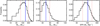Fig. D.1.

Probability distributions of $M_{tot}^{c 2}$ $M_{\mathrm{tot}}^{\mathrm{c2}}$ , $M_{tot}^{c 1}$ $M_{\mathrm{tot}}^{\mathrm{c1}}$ , and SFR in the GMF 39 (CFG047.06+0.26). The vertical blue lines show the median values and the red dashed lines mark the 1σ uncertainties.

Finally, the SFR and SFE can be obtained using the method described in Sect. 3.3.3. Repeating the above process 10 000 times, we can obtain the probability distributions for the parameters such as $M_{tot}^{c 2}$ $M_{\mathrm{tot}}^\mathrm{{c2}}$ , $M_{tot}^{c 1}$ $M_{\mathrm{tot}}^{\mathrm{c1}}$ , and SFR as shown in Fig. D.1. The blue solid lines represent the median values which we adopt as the final values of the corresponding parameters. The red dashed lines show the 1σ uncertainties. 68% scores lie between the two red dashed lines.

D.2. Uncertainty of cloud mass

The uncertainty of GMF H₂ column density is mainly from the observational random errors and the variations of T_ex and ¹³CO abundance. Compared with the last two components, the observational random errors are small and thus ignored.

Thirteen GMFs are also covered or partially covered by ThrUMMS ¹²CO survey data. For these GMFs we collapsed the corresponding data cube to obtain the ¹²CO intensity maps. Assuming the optically thick for ¹²CO (J = 1 − 0) emission lines, the excitation temperature can be obtained using the following formula (Rohlfs & Wilson 2004):

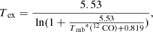
$\begin{matrix} T_{ex} = \frac{5.53}{ln (1 + \frac{5.53}{{T_{mb}}^{*} (^{12} CO) + 0.819})}, \end{matrix}$ $\begin{aligned} T_{\text{ ex}}={\frac{5.53}{{\text{ ln}} (1+\frac{5.53}{{T_{\text{ mb}}}^{*} (^{12}{\text{ CO}})+0.819})}}, \end{aligned}$

where $T_{mb}^{*} (^{12} CO)$ $T_{\mathrm{mb}}^{*} (^{12}{\mathrm{CO}})$ is obtained from the peak of the ¹²CO emission. We obtain the excitation temperature map for the region covered by ¹²CO data in each of these GMFs. Combining 13 excitation temperature maps together, Fig. D.2 shows the excitation temperature distribution. The mean value and standard deviation are ∼10 K and 2.5 K, respectively, with the minimum and maximum of 2.4 K and 33.2 K, individually. We find that the very low excitation temperatures of <4 K are mainly due to the high noise level. Thus finally we adopt a range of [4,35] K for the GMF excitation temperature. For the ¹³CO abundance of [¹³CO/H₂], previous measurements in different interstellar clouds with different conditions vary from ∼0.9 to 3.5 × 10⁻⁶ with a scatter of ∼30−50% (Dickman 1978; Frerking et al. 1982; Lada et al. 1994; Harjunpää et al. 2004; Pineda et al. 2008, 2010; Ripple et al. 2013). We ultimately assume a 50% uncertainty for the convention factor of [H₂/¹³CO] that we adopted in Appendix A.

Assuming that T_ex and [H₂/¹³CO] follow the truncated Gaussian distributions,

$\begin{matrix} T_{ex} \sim N (10, 2 . 5^{2}) 4 < T_{ex} < 35 K \end{matrix}$ $\begin{aligned} T_{\text{ ex}} \sim N(10, 2.5^2)\;\;\;\;\;\;4 <T_{\text{ ex}} < 35\,\mathrm{K} \end{aligned}$

$\begin{matrix} \frac{[H_{2} /^{13} CO]}{10^{5}} \sim N (8.5, 4 . 25^{2}) 1 < \frac{[H_{2} /^{13} CO]}{10^{5}} < 100 \end{matrix}$ $\begin{aligned} \frac{[{\text{ H}}_{\text{2}}/^{\text{13}}{\text{ CO}}]}{\text{10}^{\text{5}}} \sim N(8.5,4.25^2)\;\;\;\;\;\;1<\frac{[{\text{ H}}_{\text{2}}/^{\text{13}}{\text{ CO}}]}{\text{10}^{\text{5}}} < 100 \end{aligned}$ (D.1)

we generate one random number of T_ex and one random number of [H₂/¹³CO]. The column density map for each GMF can be obtained based on Eq. (A.1) and then the cloud mass, dense gas mass and other physical parameters of each GMF can be also obtained using the methods described in Appendices A and B. Repeating the above process 10 000 times, we can obtain the probability distributions for the parameters such as M_cloud and Σ_gas/t_ff, s as shown in Fig. D.3. We adopted the median values of the probability distributions as the final values of the corresponding parameters and 68% confidential intervals as 1σ uncertainties.

Nessie is a special case. For Nessie, we used the extinction map constructed with the technique by Kainulainen & Tan (2013) which combines a near-infrared NICER dust extinction map and a mid-infrared dust extinction map obtained based on mid-infrared absorption against the Galactic background. Kainulainen & Tan (2013) suggested that the uncertainty of the combined extinction map could be mainly from the uncertainty of NIR-MIR dust opacity ratio and they estimated that the uncertainty of this ratio is about 36% based on different dust models. Therefore, here we simply adopted an uncertainty of 36% for Nessie’s extinction map, based on which the uncertainties of other parameters such as gas mass can be obtained.

D.3. Including distance errors

The uncertainties estimated in above two sections do not include the distance errors. The uncertainties of parameters listed in Tables H.1 and H.2 do not include the distance errors, either, because distance cancels out in some quantities such as gas surface density (Σ_gas). The distances of GMFs listed in Table H.1 are directly adopted from the corresponding papers. Most of them are kinematic distances except for the GMFs from Wang et al. (2016).

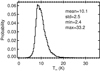Fig. D.2.

Histogram of T_ex obtained in several GMFs that are covered or partially covered by ¹²CO data.

Wang et al. (2016) use three methods to calculate the distances of their giant filaments, including trigonometric parallax measurements, maximum likelihood kinematic distance, and kinematic distance. The different methods give different uncertainties of ∼10−30% and they finally used a conservative 30% distance uncertainty. Therefore, we also decided to adopt a 30% distance uncertainty for the GMFs from Wang et al. (2016).

The kinematic distances of GMFs from other reference papers are estimated using different Galactic models. Anderson et al. (2012) analyzed the effect of different sources of the kinematic distance uncertainty. They found that the uncertainties caused by different rotation curves, non-circular motions, and the change of solar rotation parameters are about <5−20%, 5−10%, and ∼10%, respectively, and the combined uncertainty is about 20%. Roman-Duval et al. (2009) estimated the kinematic distance uncertainty through adding perturbations to the radial velocities of molecular clouds at the Galactic longitudes of 20° and 40° and obtained an uncertainty of <30%. Recently, Ramón-Fox & Bonnell (2018) investigated the gas kinematics in a spiral arm using high-resolution smoothed particle hydrodynamics simulations. They found that the kinematic distance error can be as large as ±2 kpc due to the gas streaming motions. Ramón-Fox & Bonnell (2018) also compared their results with Roman-Duval et al. (2009) and found that the relative distance errors are not larger than 30% for the clouds at galactic longitudes of ±20°. Considering these, we finally used a 30% distance uncertainty for the GMFs that are not from Wang et al. (2016). Therefore, we actually adopt a 30% distance uncertainty for all the GMFs.

Assuming the distance of each GMF, D, follows the truncated Gaussian distribution:

$\begin{matrix} D \sim N (D_{0}, {(0.3 D_{0})}^{2}) D > 1 kpc, \end{matrix}$ $\begin{aligned} D \sim N(D_0, (0.3D_0)^2)\;\;\;\;\;\;D > 1\,{\text{ kpc}}, \end{aligned}$

where D₀ represents the distance value that is listed in Table H.1, we generate one random number of D. The physical parameters of each GMF can be obtained using the dependence of parameters on distance. For example, we have obtained the probability distribution of M_cloud without considering the distance error in Appendix D.2 and thus, we are able to generate one random number, m_cloud that follows this distribution. The final total gas mass can be obtained with the relationpg of

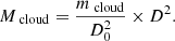
$\begin{matrix} M_{cloud} = \frac{m_{cloud}}{D_{0}^{2}} \times D^{2} . \end{matrix}$ $\begin{aligned} M_{\text{ cloud}} = \frac{m_{\text{ cloud}}}{D_0^2}\times D^2. \end{aligned}$ (D.2)

Repeating this process 10 000 times, we can obtain the probability distribution of M_cloud after including the distance error as shown in Fig. D.5 (top-right panel). The median value of this distribution is adopted as the final value of M_cloud while the 68% confidential interval is adopted as the 1σ uncertainty.

For the SFR of each GMF, it is difficult to obtain the analytical dependence on distance. We recalculate the SFRs using different distances for each GMF and the results are shown in Fig. D.4. There is roughly a linear relation between Log(SFR) and Log(Distance) (blue curves). The linear fitting results (red dashed lines) give the slope in range of [1.2, 1.4] with a mean value of 1.3. Therefore, we assume a simple relation between SFR and distance:

$\begin{matrix} SFR \propto D^{1.3} . \end{matrix}$ $\begin{aligned} {\text{ SFR}} \propto D^{1.3}. \end{aligned}$

With this relation, we were also able to obtain the probability distribution of SFR after including distance errors for each GMF as shown in Fig. D.5 (bottom-left panel).

For other more complex parameters, the dependence on distance is as follows:

$\begin{matrix} \frac{Σ_{gas}}{t_{ff,s}} \propto D^{- 0.5}, \end{matrix}$ $\begin{aligned} \frac{\Sigma _{\text{ gas}}}{{t}_{\text{ ff,s}}} \propto D^{-0.5}, \end{aligned}$ (D.3)

$\begin{matrix} \frac{Σ_{gas}}{t_{cross}} \propto D^{- 1}, \end{matrix}$ $\begin{aligned} \frac{\Sigma _{\text{ gas}}}{{t}_{\text{ cross}}} \propto D^{-1}, \end{aligned}$ (D.4)

$\begin{matrix} {SFR}_{ff,s} \propto D^{- 0.2}, \end{matrix}$ $\begin{aligned} {\text{ SFR}}_{\text{ ff,s}} \propto D^{-0.2}, \end{aligned}$ (D.5)

$\begin{matrix} SFE = \frac{1}{1 + \frac{m_{cloud}}{2 sfr} D^{0.7}}, \end{matrix}$ $\begin{aligned} {\text{ SFE}}=\frac{1}{1+\frac{m_{\text{ cloud}}}{2{\text{ sfr}}} D^{0.7}}, \end{aligned}$ (D.6)

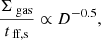
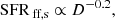
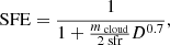
where SFR = sfrD^1.3 and M_cloud = m_cloudD². Table H.3 lists the parameters and associated uncertainties after including distance error for 34 GMFs that are located within 5.5 kpc.

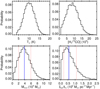Fig. D.3.

Probability distributions of T_ex, [H₂/¹³CO], M_cloud and Σ_gas/t_ff, s in the GMF 39 (CFG047.06+0.26). The vertical blue lines show the median values and the red dotted lines mark the 1σ uncertainties.

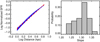Fig. D.4.

Left panel: relations between SFR and distance for 34 GMFs. Each blue curve represents one GMF. The red dashed lines show the linear fits to the blue curves; right panel: distribution of fitting slopes.

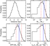Fig. D.5.

Probability distributions of distance, M_cloud, SFR, and Σ_cloud/t_ff, s in the GMF 39 (CFG047.06+0.26) after including 30% distance uncertainty. The vertical blue lines show the median values and the red dotted lines indicate the 1σ uncertainties.

Appendix E: Investigating SFR−M_dense relation with different sub-samples

In Sect. 3.3.3, we mention that we could underestimate the SFRs for the distant GMFs. Other parameters such as M_dense and length of GMFs could be also distance-biased due to the selection effects. These biases could affect the slope of SFR− M_dense relation. To investigate this, we firstly tested the correlations between the parameters such as SFR, M_dense, and length and distances of GMFs. Figure E.1 shows the result. We do not find any significant correlations between SFR, M_dense, and length versus distance for GMFs. However, due to the large uncertainties of the parameters, we can not exclude the possibility that there are strong correlations between these parameter sets, which means that we can not exclude the possibility that SFRs and M_dense of GMFs are distance-biased. We also note that there are two points away from other points in Fig. 22. These two GMFs (GMF 6 and 35) have R value of <1, which means that there are other relatively strong velocity components in the line of sight toward them and we could overestimate their SFRs. Considering above issues, we next consider the detection reliability of an approximate sublinear SFR−M_dense relation in Fig. 22.

We investigated the slope of SFR−M_dense relation in the subsequent 12 samples:

Sample 1:
GMFs (i.e., sample used in the main text).
Sample 2:
GMFs+nearby clouds.
Sample 3:
GMFs excluding GMF 6 and 35.
Sample 4:
GMFs excluding GMF 6 and 35 plus nearby clouds.
Sample 5:
GMFs with R > 1.
Sample 6:
GMFs with R > 1 plus nearby clouds.
Sample 7:
GMFs with distances of <3.5 kpc.
Sample 8:
GMFs with distances of <3.5 kpc plus nearby clouds.
Sample 9:
GMFs with distances of <4 kpc.
Sample 10:
GMFs with distances of <4 kpc plus nearby clouds.
Sample 11:
GMFs with distances of <5 kpc.
Sample 12:
GMFs with distances of <5 kpc plus nearby clouds.

Figures E.2 and E.3 shows the results. Assuming the relation of

$\begin{matrix} SFR \propto M_{dense}^{α}, \end{matrix}$ $\begin{aligned} {\text{ SFR}} \propto M_{\text{ dense}}^{\alpha }, \end{aligned}$

the slopes of α obtained with Bayesian linear regression (Kelly 2007) in different samples are shown in Fig. E.4. Although we can not exclude the possibility of α = 1, SFR−M_dense relation is sublinear within ∼68% confidence (1σ) in all 12 samples.

0

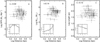Fig. E.1.

SFRs (panel a), M_dense (panel b), and length (panel c) versus distance of GMFs that are located within 5.5 kpc in the log-log plane. The correlation coefficients between different parameter sets obtained without considering uncertainties are shown at the top of each panel. The inset plots in each panel show the probability distributions of correlation coefficients (r) obtained with Bayesian linear regression method by Kelly (2007) and the vertical lines in the inset plots indicate the median values.

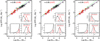Fig. E.2.

SFR as a function of M_dense for GMFs + nearby clouds (panel a); GMFs excluding two objects (GMF 6 and 35) plus nearby clouds (panel b); GMFs with R > 1 plus nearby clouds (panel c). The GMFs are marked with black filled circles while the nearby clouds are labeled with red triangles. The straight lines represent Lada’s equation (green solid line, Lada et al. 2010), the relation from Wu et al. (2005; blue dashed line), fitting result from Evans et al. (2014; red dotted line), and our linear fitting results without considering uncertainties (black solid line). The correlation coefficients between SFR and M_dense obtained without considering uncertainties are shown at the top of each panel and the black fonts are for GMFs while the red fonts are for GMFs + nearby clouds. The inset plots in each panel show the probability distributions of correlation coefficients (r), fitting slopes, and intrinsic scatters (σ) obtained with Bayesian linear regression method by Kelly (2007) for GMFs (black line) and GMFs + nearby clouds (red line).

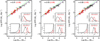Fig. E.3.

SFR as a function of M_dense for GMFs that are located within 3.5 kpc plus nearby clouds (panel a); GMFs that are located within 4 kpc plus nearby clouds (panel b); GMFs that are located within 5 kpc plus nearby clouds (panel c). The GMFs are marked with black filled circles while the nearby clouds are labeled with red triangles. The straight lines represent Lada’s equation (green solid line, Lada et al. 2010), the relation from Wu et al. (2005; blue dashed line), fitting result from Evans et al. (2014; red dotted line), and our linear fitting results without considering uncertainties (black solid line). The correlation coefficients between SFR and M_dense obtained without considering uncertainties are shown at the top of each panel and the black fonts are for GMFs while the red fonts are for GMFs + nearby clouds. The inset plots in each panel show the probability distributions of correlation coefficients (r), fitting slopes, and intrinsic scatters (σ) obtained with Bayesian linear regression method by Kelly (2007) for GMFs (black line) and GMFs + nearby clouds (red line).

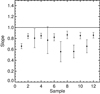Fig. E.4.

Slopes of α (black filled circles) in different samples. The black line indicates the slope = 1.

Appendix F: Plots of SFR−M relations without error bars

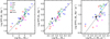Fig. F.1.

SFR and SFR/L as a function of dense gas mass (left panel), cloud mass (middle panel), and dense gas mass per unit length (right panel) for GMFs from different original publications. The black solid lines represent the linear fitting results for all data points. We do not plot error bars with the aim to show different symbols more clearly.

Appendix G: Image gallery

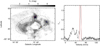Fig. G.1.

Overview of GMF 1 (G015.653−0.224). Left panel: background is CO-based extinction map. The black and blue contours represent the visual extinction of A_V = 3 and 7 mag, individually. The dashed ellipses are obtained through fitting the pixels inside the regions with A_V > 3 mag. The identified YSOs are labeled with red filled circles (Class I) and green pluses (Class II). Right panel: ¹³CO average spectrum for the region with A_V > 3 mag. The red vertical lines show the GMF velocity range (see Figs. G.2–G.49).

Fig. G.2.

Overview of GMF 2 (F19). Others are the same as Fig. G.1.

Fig. G.3.

Overview of GMF 3 (GMF20.0−17.9). Others are the same as Fig. G.1.

Fig. G.4.

Overview of GMF 4 (F20). Others are the same as Fig. G.1.

Fig. G.5.

Overview of GMF 5 (G021.173−0.312). Others are the same as Fig. G.1.

Fig. G.6.

Overview of GMF 6 (BC_021.25−0.15). Others are the same as Fig. G.1.

Fig. G.7.

Overview of GMF 7 (G022.519−0.025). Others are the same as Fig. G.1.

Fig. G.8.

Overview of GMF 8 (F21). Others are the same as Fig. G.1.

Fig. G.9.

Overview of GMF 9 (F23). Others are the same as Fig. G.1.

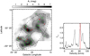Fig. G.10.

Overview of GMF 10 (F24). Others are the same as Fig. G.1.

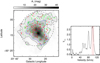Fig. G.11.

Overview of GMF 11 (F22). Others are the same as Fig. G.1.

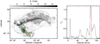Fig. G.12.

Overview of GMF 12 (CFG024.00+0.48). Others are the same as Fig. G.1.

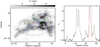Fig. G.13.

Overview of GMF 13 (F26). Others are the same as Fig. G.1.

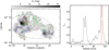Fig. G.14.

Overview of GMF 14 (F27). Others are the same as Fig. G.1.

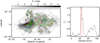Fig. G.15.

Overview of GMF 15 (BC_24.95−0.17). Others are the same as Fig. G.1.

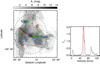Fig. G.16.

Overview of GMF 16 (BC_025.24−0.45). Others are the same as Fig. G.1.

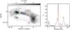Fig. G.17.

Overview of GMF 17 (F28). Others are the same as Fig. G.1.

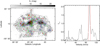Fig. G.18.

Overview of GMF 18 (F29). Others are the same as Fig. G.1.

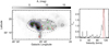Fig. G.19.

Overview of GMF 19 (G025.762+0.241). Others are the same as Fig. G.1.

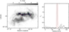Fig. G.20.

Overview of GMF 20 (BC_26.94−0.30). Others are the same as Fig. G.1.

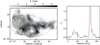Fig. G.21.

Overview of GMF 21 (F30). Others are the same as Fig. G.1.

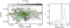Fig. G.22.

Overview of GMF 22 (F31). Others are the same as Fig. G.1.

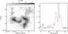Fig. G.23.

Overview of GMF 23 (CFG028.68−0.28). Others are the same as Fig. G.1.

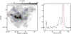Fig. G.24.

Overview of GMF 24 (G028.854−0.238). Others are the same as Fig. G.1.

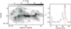Fig. G.25.

Overview of GMF 25 (CFG029.18−0.34). Others are the same as Fig. G.1.

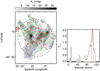Fig. G.26.

Overview of GMF 26 (G030.315−0.154). Others are the same as Fig. G.1.

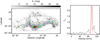Fig. G.27.

Overview of GMF 27 (G32.02+0.06). Others are the same as Fig. G.1.

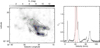Fig. G.28.

Overview of GMF 28 (G032.401+0.082). Others are the same as Fig. G.1.

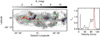Fig. G.29.

Overview of GMF 29 (F34). Others are the same as Fig. G.1.

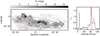Fig. G.30.

Overview of GMF 30 (G033.104+0.068). Others are the same as Fig. G.1.

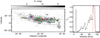Fig. G.31.

Overview of GMF 31 (G033.685−0.020). Others are the same as Fig. G.1.

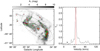Fig. G.32.

Overview of GMF 32 (GMF38.1−32.4b). Others are the same as Fig. G.1.

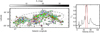Fig. G.33.

Overview of GMF 33 (GMF38.1−32.4a). Others are the same as Fig. G.1.

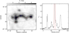Fig. G.34.

Overview of GMF 34 (G037.410−0.070). Others are the same as Fig. G.1.

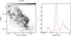Fig. G.35.

Overview of GMF 35 (GMF41.0−41.3). Others are the same as Fig. G.1.

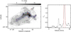Fig. G.36.

Overview of GMF 36 (F38). Others are the same as Fig. G.1.

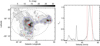Fig. G.37.

Overview of GMF 37 (F39). Others are the same as Fig. G.1.

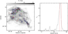Fig. G.38.

Overview of GMF 38 (F40). Others are the same as Fig. G.1.

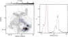Fig. G.39.

Overview of GMF 40 (G048.629+0.096). Others are the same as Fig. G.1.

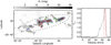Fig. G.40.

Overview of GMF 41 (CFG049.21−0.34). Others are the same as Fig. G.1.

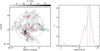Fig. G.41.

Overview of GMF 42 (F42). Others are the same as Fig. G.1.

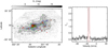Fig. G.42.

Overview of GMF 47 (GMF324.5−321.4b). Others are the same as Fig. G.1.

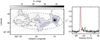Fig. G.43.

Overview of GMF 48 (G322.363+0.542). Others are the same as Fig. G.1.

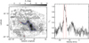Fig. G.44.

Overview of GMF 49 (G323.929+0.036). Others are the same as Fig. G.1.

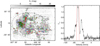Fig. G.45.

Overview of GMF 50 (G327.157−0.256). Others are the same as Fig. G.1.

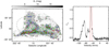Fig. G.46.

Overview of GMF 51 (GMF335.6−333.6b). Others are the same as Fig. G.1.

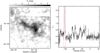Fig. G.47.

Overview of GMF 55 (G341.938+0.054). Others are the same as Fig. G.1.

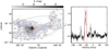Fig. G.48.

Overview of GMF 56 (G349.876+0.099). Others are the same as Fig. G.1.

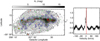Fig. G.49.

Overview of GMF 57 (GMF358.9−357.4). Others are the same as Fig. G.1.

Appendix H: Additional tables

Table H.1.

Physical parameters of the Galactic giant molecular filaments.

Table H.2.

YSO content of the Galactic giant molecular filaments.

Table H.3.

Parameters and associated uncertainties of the Galactic giant molecular filaments.

All Tables

Table 1.

Summary of data used in this paper.

In the text

Table 2.

Summary of giant filaments identified with different dataset and criteria.

In the text

Table 3.

Properties of nearby molecular clouds.

In the text

Table H.1.

Physical parameters of the Galactic giant molecular filaments.

In the text

Table H.2.

YSO content of the Galactic giant molecular filaments.

In the text

Table H.3.

Parameters and associated uncertainties of the Galactic giant molecular filaments.

In the text

All Figures

	Fig. 1. Flow chart of our automatic PSF-fitting pipeline that is used to do the PSF photometry on the VVV survey imaging data.
In the text

	Fig. 2. K_s magnitude distributions of the sources detected by PSF photometry (black line) and sources in VVV CASU catalog (red line) for tile “b332” (left panel) and tile “d095” (right panel).
In the text

Fig. 3.

Overview of GMF 39 (CFG047.06+0.26). Left panel: background is CO-based extinction map. The black and blue contours represent the visual extinction of A_V = 3 and 7 mag, individually. The dashed ellipses are obtained through fitting the pixels inside the regions with A_V > 3 mag. The identified YSOs are labeled with red filled circles (Class I) and green pluses (Class II). Right panel: ¹³CO average spectrum for the region with A_V > 3 mag. The red vertical lines mark the GMF velocity range.

In the text

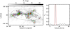	Fig. 4. Overview of GMF 43 (GMF54.0−52.0). Others are same as Fig. 3.
In the text

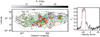	Fig. 5. Overview of GMF 44 (GMF307.2−305.4). Others are same as Fig. 3.
In the text

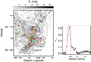	Fig. 6. Overview of GMF 45 (GMF309.5−308.7). Others are same as Fig. 3.
In the text

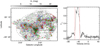	Fig. 7. Overview of GMF 46 (GMF319.0−318.7). Others are same as Fig. 3.
In the text

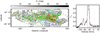	Fig. 8. Overview of GMF 52 (GMF335.6−333.6a). Others are same as Fig. 3.
In the text

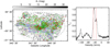	Fig. 9. Overview of GMF 54 (GMF341.9−337.1). Others are same as Fig. 3.
In the text

Fig. 10.

H − K_s versus J − H color–color diagram for the YSOs in the GMF 39 (CFG047.06+0.26). The solid curves show the intrinsic colors for the main-sequence stars (black) and giants (red; Bessell & Brett 1988), and the dash-dotted line is the locus of T Tauri stars from Meyer et al. (1997). The dashed lines show the reddening direction, and the arrow shows the reddening vector. The extinction law we adopted is from Xue et al. (2016). We note that the dashed lines separate the diagram into three regions marked with numbers 1, 2, and 3 in the figure. We use different methods to estimate the extinction of YSOs in different regions (see the text for details).

In the text

	Fig. 11. Dereddened α and T_bol of YSOs in the GMF 39 (CFG047.06+0.26). The dashed lines show the boundaries of YSO classification schemes (Greene et al. 1994; Chen et al. 1995).
In the text

	Fig. 12. K_s absolute magnitude (M_{K_s}) histogram of Class II sources in GMF 46 (GMF319.0−318.7).
In the text

Fig. 13.

Relation between stellar mass and K_s absolute magnitude of Class II source. The black dots represent the Robitaille et al. (2006) Stage 2 models with 0.001 < M_disk/M_* < 0.01, 0.08 < M_* < 7 M_⊙, and 30 ° < inclination angle < 60°. The red curve shows the robust polynomial fitting while the gray region shows the 1σ uncertainty of the fitting. The CTTS in L1641 from Fang et al. (2013) are marked with green filled circles.

In the text

	Fig. 14. Dereddened luminosity functions constructed by Kryukova et al. (2012) for the combined low-mass star-forming clouds (left) and combined high-mass star-forming clouds (right). The red vertical lines show the dereddened L_cut.
In the text

	Fig. 15. Dereddened luminosity function of Class I sources in GMF 46 (GMF319.0−318.7). The red vertical line shows the dereddened L_cut.
In the text

	Fig. 16. Spatial distribution of 57 Galactic GMFs. The backgrounds are ¹³CO intensity maps of the GRS and ThrUMMS data, integrated over the entire observed velocity range. The red ellipses mark the positions of 57 GMFs. We obtained the star formation rates of 46 GMFs (see Sect. 3.3 for details) that are labeled with green pluses.
In the text

Fig. 17.

Distributions of filament length (panel a); heliocentric distance (panel b); logarithm of cloud mass M_cloud (panel c); line width Δv (panel d); logarithm of gas surface density Σ_gas (panel e); logarithm of dense gas mass M_dense (panel f); free-fall time obtained based on spherical morphology (panel g); aspect ratio (panel h); and logarithm of dense gas mass per unit length (panel i).

In the text

Fig. 18.

¹³CO line widths vs. sizes (left panel) and masses (right panel) of the GMFs in log-log plane. The solid lines show the best linear fittings to the points without considering the uncertainties. The correlation coefficients and the fitting results that are obtained without considering the uncertainties are also marked in the top region of panels. The small inset plots in each panel show the probability distributions of correlation coefficients and fitting slopes that are obtained after including uncertainties on both axes using the Bayesian linear regression method developed by Kelly (2007).

In the text

	Fig. 19. Two-point correlation functions for the Class I sources in 6 GMFs. The title on each panel corresponds to the ID number of Table H.2. The red solid lines show the linear fits to the roughly straight line part of the data and the fitting slopes are labeled in each panel.
In the text

	Fig. 20. Probability distributions of star formation rate (panel a); star formation efficiency (panel b); surface density of star formation rate for 34 GMFs with the distances of <5.5 kpc (panel c). The red vertical lines show the median values of SFE and Σ_SFR that are re-estimated with Class I+Flat+II sources in the nearby star-forming regions (see the text for details).
In the text

Fig. 21.

Surface density of SFR, Σ_SFR, as a function of Σ_gas (panel a), Σ_gas/t_ff, s (panel b), Σ_gas/t_cross (panel c), and Σ_gas/t_ff, f (panel d) for the Galactic GMFs (black filled circles) and the nearby star-forming regions (red triangles). The lines in panel a correspond to the star formation relations suggested by Kennicutt (1998, green solid) and Bigiel et al. (2008, blue dashed). The lines in panels b and d correspond to star formation law suggested by Krumholz et al. (2012) with ϵ_ff = 0.001, 0.01, and 0.1, respectively. The Pearson correlation coefficients between the different sets of parameters obtained without considering uncertainties are marked on top region of each panel and the black fonts are for GMFs while the red fonts are for GMFs + nearby clouds. The inset plots in each panel show probability distributions of correlation coefficients (r) obtained with Bayesian linear regression method by Kelly (2007) for GMFs (black line) and GMFs + nearby clouds (red line).

In the text

Fig. 22.

SFR and Σ_SFR as a function of dense gas mass (panel a); cloud mass (panel b); and f_DGΣ_gas for GMFs (panel c). The GMFs from different original identification publications are marked with different symbols. The abbreviations correspond to the column one of Table 2. The straight lines represent Lada’s equation (green solid line, Lada et al. 2010), the relation from Wu et al. (2005; blue dashed line), fitting result from Evans et al. (2014; red dotted line), and our linear fitting results without considering uncertainties (black solid line). The Pearson correlation coefficients between the different sets of parameters obtained without considering uncertainties are marked on top region of each panel. The inset plots in each panel show the probability distributions of correlation coefficients (r), fitting slopes, and intrinsic scatters (σ) obtained with Bayesian linear regression method by Kelly (2007).

In the text

Fig. 23.

SFR/M_dense as a function of dense gas mass for the GMFs. GMFs from different original identification publications are marked with different symbols. The abbreviations correspond to the column one of Table 2. The Pearson r obtained without considering uncertainties is marked on the top of the figure. The inset plots show the probability distributions of correlation coefficient and fitting slope obtained with Bayesian linear regression method by Kelly (2007).

In the text

Fig. 24.

SFR per unit length vs. dense gas mass per unit length for GMFs. GMFs from different original identification publications are marked with different symbols. The abbreviations correspond to the column one of Table 2. The black line shows the linear fittings obtained without considering uncertainties. The Pearson r obtained without considering uncertainties is also marked on the top of the figure. The inset plots show the probability distributions of correlation coefficient and fitting slope obtained with Bayesian linear regression method by Kelly (2007).

In the text

Fig. 25.

SFR per unit length vs. Class II to Class I YSO fraction for the GMFs (left panel) and the nearby star-forming clouds (right panel). The Pearson r values obtained without considering uncertainty are marked on the top of panels. The inset plots in each panel show the probability distributions of correlations coefficient and fitting slope obtained with Bayesian linear regression method by Kelly (2007).

In the text

	Fig. A.1. ¹³CO average spectrum of GMF 20 (i.e., BC_026.94−0.30) that is identified originally by Zucker et al. (2015). The red curve shows the best fitting using the multiple Gaussian components. The dashed line marks the central velocity offered by Zucker et al. (2015) and the blue solid lines show the velocity range of this component.
In the text

	Fig. B.1. ¹³CO line width distribution map (obtained from the moment 2 map) of GMF 39 (CFG047.06+0.26).
In the text

Fig. C.1.

Color–color diagrams used for identification of Class I (left), and Class II (right) sources in phase 1 of the classification scheme presented by Gutermuth et al. (2009) for an example of GMF 39 (CFG047.06+0.26). The black filled circles represent the selected Class I and Class II sources. The remaining Class III/field sources are indicated by the gray dots. The black lines show the color criteria of the classification scheme.

In the text

Fig. C.2.

Color–color diagrams used for YSO identification in phase 2 (panel a) and phase 3 (panels b and c) classification schemes suggested by Gutermuth et al. (2009) for an example of GMF 39 (CFG047.06+0.26). The Class I sources identified in phase 2 and the protostars identified in phase 3 are marked with red dots. The Class II sources isolated in phase 2 are labeled with green dots while the transition disks classified in phase 3 are shown with blue dots.

In the text

	Fig. C.3. Color criteria used to isolate the possible AGB stars from the YSOs in Step 3 for an example of GMF 39 (CFG047.06+0.26). The red dots indicate the Class I sources or protostars while the green and blue dots label the Class II and transition disks, respectively. The AGBs are marked with black dots. The black solid lines show the boundaries of the classification criteria.
In the text

	Fig. C.4. Color–color diagrams and the color-magnitude diagram used in Step 4 for a example of GMF 39 (CFG047.06+0.26). The red dots indicate the Class I sources and protostars identified in the YSO classification scheme suggested by Koenig & Leisawitz (2014) while the green and blue dots label the Class II sources and transition disks, respectively.
In the text

	Fig. C.5. Color-magnitude and color–color diagrams used to isolate the possible AGBs from YSOs in Step 4 for an example of GMF 39 (CFG047.06+0.26).
In the text

	Fig. D.1. Probability distributions of $M_{tot}^{c 2}$ $M_{\mathrm{tot}}^{\mathrm{c2}}$ , $M_{tot}^{c 1}$ $M_{\mathrm{tot}}^{\mathrm{c1}}$ , and SFR in the GMF 39 (CFG047.06+0.26). The vertical blue lines show the median values and the red dashed lines mark the 1σ uncertainties.
In the text

	Fig. D.2. Histogram of T_ex obtained in several GMFs that are covered or partially covered by ¹²CO data.
In the text

	Fig. D.3. Probability distributions of T_ex, [H₂/¹³CO], M_cloud and Σ_gas/t_ff, s in the GMF 39 (CFG047.06+0.26). The vertical blue lines show the median values and the red dotted lines mark the 1σ uncertainties.
In the text

	Fig. D.4. Left panel: relations between SFR and distance for 34 GMFs. Each blue curve represents one GMF. The red dashed lines show the linear fits to the blue curves; right panel: distribution of fitting slopes.
In the text

	Fig. D.5. Probability distributions of distance, M_cloud, SFR, and Σ_cloud/t_ff, s in the GMF 39 (CFG047.06+0.26) after including 30% distance uncertainty. The vertical blue lines show the median values and the red dotted lines indicate the 1σ uncertainties.
In the text

Fig. E.1.

SFRs (panel a), M_dense (panel b), and length (panel c) versus distance of GMFs that are located within 5.5 kpc in the log-log plane. The correlation coefficients between different parameter sets obtained without considering uncertainties are shown at the top of each panel. The inset plots in each panel show the probability distributions of correlation coefficients (r) obtained with Bayesian linear regression method by Kelly (2007) and the vertical lines in the inset plots indicate the median values.

In the text

Fig. E.2.

SFR as a function of M_dense for GMFs + nearby clouds (panel a); GMFs excluding two objects (GMF 6 and 35) plus nearby clouds (panel b); GMFs with R > 1 plus nearby clouds (panel c). The GMFs are marked with black filled circles while the nearby clouds are labeled with red triangles. The straight lines represent Lada’s equation (green solid line, Lada et al. 2010), the relation from Wu et al. (2005; blue dashed line), fitting result from Evans et al. (2014; red dotted line), and our linear fitting results without considering uncertainties (black solid line). The correlation coefficients between SFR and M_dense obtained without considering uncertainties are shown at the top of each panel and the black fonts are for GMFs while the red fonts are for GMFs + nearby clouds. The inset plots in each panel show the probability distributions of correlation coefficients (r), fitting slopes, and intrinsic scatters (σ) obtained with Bayesian linear regression method by Kelly (2007) for GMFs (black line) and GMFs + nearby clouds (red line).

In the text

Fig. E.3.

SFR as a function of M_dense for GMFs that are located within 3.5 kpc plus nearby clouds (panel a); GMFs that are located within 4 kpc plus nearby clouds (panel b); GMFs that are located within 5 kpc plus nearby clouds (panel c). The GMFs are marked with black filled circles while the nearby clouds are labeled with red triangles. The straight lines represent Lada’s equation (green solid line, Lada et al. 2010), the relation from Wu et al. (2005; blue dashed line), fitting result from Evans et al. (2014; red dotted line), and our linear fitting results without considering uncertainties (black solid line). The correlation coefficients between SFR and M_dense obtained without considering uncertainties are shown at the top of each panel and the black fonts are for GMFs while the red fonts are for GMFs + nearby clouds. The inset plots in each panel show the probability distributions of correlation coefficients (r), fitting slopes, and intrinsic scatters (σ) obtained with Bayesian linear regression method by Kelly (2007) for GMFs (black line) and GMFs + nearby clouds (red line).

In the text

	Fig. E.4. Slopes of α (black filled circles) in different samples. The black line indicates the slope = 1.
In the text

	Fig. F.1. SFR and SFR/L as a function of dense gas mass (left panel), cloud mass (middle panel), and dense gas mass per unit length (right panel) for GMFs from different original publications. The black solid lines represent the linear fitting results for all data points. We do not plot error bars with the aim to show different symbols more clearly.
In the text

Fig. G.1.

Overview of GMF 1 (G015.653−0.224). Left panel: background is CO-based extinction map. The black and blue contours represent the visual extinction of A_V = 3 and 7 mag, individually. The dashed ellipses are obtained through fitting the pixels inside the regions with A_V > 3 mag. The identified YSOs are labeled with red filled circles (Class I) and green pluses (Class II). Right panel: ¹³CO average spectrum for the region with A_V > 3 mag. The red vertical lines show the GMF velocity range (see Figs. G.2–G.49).

In the text

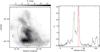	Fig. G.2. Overview of GMF 2 (F19). Others are the same as Fig. G.1.
In the text

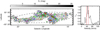	Fig. G.3. Overview of GMF 3 (GMF20.0−17.9). Others are the same as Fig. G.1.
In the text

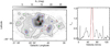	Fig. G.4. Overview of GMF 4 (F20). Others are the same as Fig. G.1.
In the text

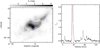	Fig. G.5. Overview of GMF 5 (G021.173−0.312). Others are the same as Fig. G.1.
In the text

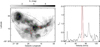	Fig. G.6. Overview of GMF 6 (BC_021.25−0.15). Others are the same as Fig. G.1.
In the text

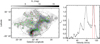	Fig. G.7. Overview of GMF 7 (G022.519−0.025). Others are the same as Fig. G.1.
In the text

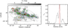	Fig. G.8. Overview of GMF 8 (F21). Others are the same as Fig. G.1.
In the text

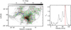	Fig. G.9. Overview of GMF 9 (F23). Others are the same as Fig. G.1.
In the text

	Fig. G.10. Overview of GMF 10 (F24). Others are the same as Fig. G.1.
In the text

	Fig. G.11. Overview of GMF 11 (F22). Others are the same as Fig. G.1.
In the text

	Fig. G.12. Overview of GMF 12 (CFG024.00+0.48). Others are the same as Fig. G.1.
In the text

	Fig. G.13. Overview of GMF 13 (F26). Others are the same as Fig. G.1.
In the text

	Fig. G.14. Overview of GMF 14 (F27). Others are the same as Fig. G.1.
In the text

	Fig. G.15. Overview of GMF 15 (BC_24.95−0.17). Others are the same as Fig. G.1.
In the text

	Fig. G.16. Overview of GMF 16 (BC_025.24−0.45). Others are the same as Fig. G.1.
In the text

	Fig. G.17. Overview of GMF 17 (F28). Others are the same as Fig. G.1.
In the text

	Fig. G.18. Overview of GMF 18 (F29). Others are the same as Fig. G.1.
In the text

	Fig. G.19. Overview of GMF 19 (G025.762+0.241). Others are the same as Fig. G.1.
In the text

	Fig. G.20. Overview of GMF 20 (BC_26.94−0.30). Others are the same as Fig. G.1.
In the text

	Fig. G.21. Overview of GMF 21 (F30). Others are the same as Fig. G.1.
In the text

	Fig. G.22. Overview of GMF 22 (F31). Others are the same as Fig. G.1.
In the text

	Fig. G.23. Overview of GMF 23 (CFG028.68−0.28). Others are the same as Fig. G.1.
In the text

	Fig. G.24. Overview of GMF 24 (G028.854−0.238). Others are the same as Fig. G.1.
In the text

	Fig. G.25. Overview of GMF 25 (CFG029.18−0.34). Others are the same as Fig. G.1.
In the text

	Fig. G.26. Overview of GMF 26 (G030.315−0.154). Others are the same as Fig. G.1.
In the text

	Fig. G.27. Overview of GMF 27 (G32.02+0.06). Others are the same as Fig. G.1.
In the text

	Fig. G.28. Overview of GMF 28 (G032.401+0.082). Others are the same as Fig. G.1.
In the text

	Fig. G.29. Overview of GMF 29 (F34). Others are the same as Fig. G.1.
In the text

	Fig. G.30. Overview of GMF 30 (G033.104+0.068). Others are the same as Fig. G.1.
In the text

	Fig. G.31. Overview of GMF 31 (G033.685−0.020). Others are the same as Fig. G.1.
In the text

	Fig. G.32. Overview of GMF 32 (GMF38.1−32.4b). Others are the same as Fig. G.1.
In the text

	Fig. G.33. Overview of GMF 33 (GMF38.1−32.4a). Others are the same as Fig. G.1.
In the text

	Fig. G.34. Overview of GMF 34 (G037.410−0.070). Others are the same as Fig. G.1.
In the text

	Fig. G.35. Overview of GMF 35 (GMF41.0−41.3). Others are the same as Fig. G.1.
In the text

	Fig. G.36. Overview of GMF 36 (F38). Others are the same as Fig. G.1.
In the text

	Fig. G.37. Overview of GMF 37 (F39). Others are the same as Fig. G.1.
In the text

	Fig. G.38. Overview of GMF 38 (F40). Others are the same as Fig. G.1.
In the text

	Fig. G.39. Overview of GMF 40 (G048.629+0.096). Others are the same as Fig. G.1.
In the text

	Fig. G.40. Overview of GMF 41 (CFG049.21−0.34). Others are the same as Fig. G.1.
In the text

	Fig. G.41. Overview of GMF 42 (F42). Others are the same as Fig. G.1.
In the text

	Fig. G.42. Overview of GMF 47 (GMF324.5−321.4b). Others are the same as Fig. G.1.
In the text

	Fig. G.43. Overview of GMF 48 (G322.363+0.542). Others are the same as Fig. G.1.
In the text

	Fig. G.44. Overview of GMF 49 (G323.929+0.036). Others are the same as Fig. G.1.
In the text

	Fig. G.45. Overview of GMF 50 (G327.157−0.256). Others are the same as Fig. G.1.
In the text

	Fig. G.46. Overview of GMF 51 (GMF335.6−333.6b). Others are the same as Fig. G.1.
In the text

	Fig. G.47. Overview of GMF 55 (G341.938+0.054). Others are the same as Fig. G.1.
In the text

	Fig. G.48. Overview of GMF 56 (G349.876+0.099). Others are the same as Fig. G.1.
In the text

	Fig. G.49. Overview of GMF 57 (GMF358.9−357.4). Others are the same as Fig. G.1.
In the text

Current usage metrics show cumulative count of Article Views (full-text article views including HTML views, PDF and ePub downloads, according to the available data) and Abstracts Views on Vision4Press platform.

Data correspond to usage on the plateform after 2015. The current usage metrics is available 48-96 hours after online publication and is updated daily on week days.

Initial download of the metrics may take a while.

[1] Abergel, A., Boulanger, F., Mizuno, A., & Fukui, Y. 1994, ApJ, 423, L59 [NASA ADS] [CrossRef] [Google Scholar]

[2] Abreu-Vicente, J., Ragan, S., Kainulainen, J., et al. 2016, A&A, 590, A131 [NASA ADS] [CrossRef] [EDP Sciences] [Google Scholar]

[3] Alfaro, E. J., & Sánchez, N. 2011, in Computational Star Formation, eds. J. Alves, B. G. Elmegreen, J. M. Girart, & V. Trimble, IAU Symp., 270, 81 [NASA ADS] [Google Scholar]

[4] Alves de Oliveira, C., Schneider, N., Merín, B., et al. 2014, A&A, 568, A98 [NASA ADS] [CrossRef] [EDP Sciences] [Google Scholar]

[5] Anderson, L. D., Bania, T. M., Balser, D. S., & Rood, R. T. 2012, ApJ, 754, 62 [NASA ADS] [CrossRef] [Google Scholar]

[6] André, P., Men’shchikov, A., Bontemps, S., et al. 2010, A&A, 518, L102 [NASA ADS] [CrossRef] [EDP Sciences] [Google Scholar]

[7] André, P., Di Francesco, J., Ward-Thompson, D., et al. 2014, Protostars and Planets VI, 27 [Google Scholar]

[8] Andrews, S. M., Rosenfeld, K. A., Kraus, A. L., & Wilner, D. J. 2013, ApJ, 771, 129 [NASA ADS] [CrossRef] [Google Scholar]

[9] Antoniucci, S., García López, R., Nisini, B., et al. 2014, A&A, 572, A62 [NASA ADS] [CrossRef] [EDP Sciences] [Google Scholar]

[10] Arzoumanian, D., André, P., Didelon, P., et al. 2011, A&A, 529, L6 [Google Scholar]

[11] Bally, J., Langer, W. D., Stark, A. A., & Wilson, R. W. 1987, ApJ, 312, L45 [NASA ADS] [CrossRef] [Google Scholar]

[12] Barnard, E. E., Frost, E. B., & Calvert, M. R. 1927, A Photographic Atlas of Selected Regions of the Milky Way (Washington: Carnegie Institution of Washington) [Google Scholar]

[13] Barnes, P. J., Muller, E., Indermuehle, B., et al. 2015, ApJ, 812, 6 [NASA ADS] [CrossRef] [Google Scholar]

[14] Belloche, A., Schuller, F., Parise, B., et al. 2011, A&A, 527, A145 [NASA ADS] [CrossRef] [EDP Sciences] [Google Scholar]

[15] Benjamin, R. A., Churchwell, E., Babler, B. L., et al. 2003, PASP, 115, 953 [NASA ADS] [CrossRef] [Google Scholar]

[16] Bessell, M. S., & Brett, J. M. 1988, PASP, 100, 1134 [NASA ADS] [CrossRef] [Google Scholar]

[17] Bigiel, F., Leroy, A., Walter, F., et al. 2008, AJ, 136, 2846 [NASA ADS] [CrossRef] [Google Scholar]

[18] Binney, J., & Tremaine, S. 1987, Galactic Dynamics (Princeton: Princeton University Press) [Google Scholar]

[19] Bohlin, R. C., Savage, B. D., & Drake, J. F. 1978, ApJ, 224, 132 [NASA ADS] [CrossRef] [Google Scholar]

[20] Bontemps, S., André, P., Könyves, V., et al. 2010, A&A, 518, L85 [NASA ADS] [CrossRef] [EDP Sciences] [Google Scholar]

[21] Bourke, T. L., Garay, G., Lehtinen, K. K., et al. 1997, ApJ, 476, 781 [NASA ADS] [CrossRef] [Google Scholar]

[22] Butler, M. J., & Tan, J. C. 2012, ApJ, 754, 5 [NASA ADS] [CrossRef] [Google Scholar]

[23] Cambrésy, L. 1999, A&A, 345, 965 [NASA ADS] [Google Scholar]

[24] Caratti o Garatti, A., Garcia Lopez, R., Antoniucci, S., et al. 2012, A&A, 538, A64 [NASA ADS] [CrossRef] [EDP Sciences] [Google Scholar]

[25] Carey, S. J., Noriega-Crespo, A., Mizuno, D. R., et al. 2009, PASP, 121, 76 [NASA ADS] [CrossRef] [Google Scholar]

[26] Casali, M., Adamson, A., Alves de Oliveira, C., et al. 2007, A&A, 467, 777 [NASA ADS] [CrossRef] [EDP Sciences] [Google Scholar]

[27] Chen, H., Myers, P. C., Ladd, E. F., & Wood, D. O. S. 1995, ApJ, 445, 377 [NASA ADS] [CrossRef] [Google Scholar]

[28] Churchwell, E., Babler, B. L., Meade, M. R., et al. 2009, PASP, 121, 213 [NASA ADS] [CrossRef] [Google Scholar]

[29] Comerón, F. 2008, in The Lupus Clouds, ed. B. Reipurth, 295 [Google Scholar]

[30] Cox, N. L. J., Arzoumanian, D., André, P., et al. 2016, A&A, 590, A110 [NASA ADS] [CrossRef] [EDP Sciences] [Google Scholar]

[31] Dalton, G. B., Caldwell, M., Ward, A. K., et al. 2006, in Society of Photo-Optical Instrumentation Engineers (SPIE) Conference Series, Proc. SPIE, 6269, 62690X [Google Scholar]

[32] de Geus, E. J., de Zeeuw, P. T., & Lub, J. 1989, A&A, 216, 44 [NASA ADS] [Google Scholar]

[33] Dickman, R. L. 1978, ApJS, 37, 407 [NASA ADS] [CrossRef] [Google Scholar]

[34] Du, F., & Yang, J. 2008, ApJ, 686, 384 [NASA ADS] [CrossRef] [Google Scholar]

[35] Duarte-Cabral, A., & Dobbs, C. L. 2017, MNRAS, 470, 4261 [NASA ADS] [CrossRef] [Google Scholar]

[36] Dunham, M. M., Crapsi, A., Evans, II., N. J., et al. 2008, ApJS, 179, 249 [NASA ADS] [CrossRef] [Google Scholar]

[37] Dunham, M. M., Stutz, A. M., Allen, L. E., et al. 2014, Protostars and Planets VI, 195 [Google Scholar]

[38] Dunham, M. M., Allen, L. E., Evans, II., N. J., et al. 2015, ApJS, 220, 11 [NASA ADS] [CrossRef] [Google Scholar]

[39] Dzib, S., Loinard, L., Mioduszewski, A. J., et al. 2010, ApJ, 718, 610 [NASA ADS] [CrossRef] [Google Scholar]

[40] Dzib, S., Loinard, L., Mioduszewski, A. J., et al. 2011, Rev. Mex. Astron. Astrofis. Conf. Ser., 40, 231 [NASA ADS] [Google Scholar]

[41] Eden, D. J., Moore, T. J. T., Morgan, L. K., Thompson, M. A., & Urquhart, J. S. 2013, MNRAS, 431, 1587 [NASA ADS] [CrossRef] [Google Scholar]

[42] Elia, D., Molinari, S., Fukui, Y., et al. 2013, ApJ, 772, 45 [NASA ADS] [CrossRef] [Google Scholar]

[43] Emerson, J. P., & Sutherland, W. J. 2010, in Ground-based and Airborne Telescopes III, Proc. SPIE, 7733, 773306 [CrossRef] [Google Scholar]

[44] Enoch, M. L., Young, K. E., Glenn, J., et al. 2006, ApJ, 638, 293 [NASA ADS] [CrossRef] [Google Scholar]

[45] Evans, N. J., Dunham, M. M., Jørgensen, J. K., et al. 2009, ApJS, 181, 321 [NASA ADS] [CrossRef] [Google Scholar]

[46] Evans, II., N. J., Heiderman, A., & Vutisalchavakul, N. 2014, ApJ, 782, 114 [NASA ADS] [CrossRef] [Google Scholar]

[47] Fang, M., Kim, J. S., van Boekel, R., et al. 2013, ApJS, 207, 5 [NASA ADS] [CrossRef] [Google Scholar]

[48] Fernández-López, M., Arce, H. G., Looney, L., et al. 2014, ApJ, 790, L19 [NASA ADS] [CrossRef] [Google Scholar]

[49] Fiege, J. D., & Pudritz, R. E. 2000, MNRAS, 311, 85 [NASA ADS] [CrossRef] [Google Scholar]

[50] Fischera, J., & Martin, P. G. 2012, A&A, 542, A77 [NASA ADS] [CrossRef] [EDP Sciences] [Google Scholar]

[51] Foyle, K., Rix, H.-W., Walter, F., & Leroy, A. K. 2010, ApJ, 725, 534 [NASA ADS] [CrossRef] [Google Scholar]

[52] Franco, G. A. P. 1991, A&A, 251, 581 [NASA ADS] [Google Scholar]

[53] Frerking, M. A., Langer, W. D., & Wilson, R. W. 1982, ApJ, 262, 590 [NASA ADS] [CrossRef] [Google Scholar]

[54] Gaczkowski, B., Preibisch, T., Ratzka, T., et al. 2013, A&A, 549, A67 [NASA ADS] [CrossRef] [EDP Sciences] [Google Scholar]

[55] Gao, Y., & Solomon, P. M. 2004, ApJ, 606, 271 [NASA ADS] [CrossRef] [Google Scholar]

[56] Garden, R. P., Hayashi, M., Hasegawa, T., Gatley, I., & Kaifu, N. 1991, ApJ, 374, 540 [NASA ADS] [CrossRef] [Google Scholar]

[57] Giannini, T., Elia, D., Lorenzetti, D., et al. 2012, A&A, 539, A156 [NASA ADS] [CrossRef] [EDP Sciences] [Google Scholar]

[58] Gomez, M., Hartmann, L., Kenyon, S. J., & Hewett, R. 1993, AJ, 105, 1927 [NASA ADS] [CrossRef] [Google Scholar]

[59] Gong, Y., Mao, R. Q., Fang, M., et al. 2016, A&A, 588, A104 [NASA ADS] [CrossRef] [EDP Sciences] [Google Scholar]

[60] Goodman, A. A., Pineda, J. E., & Schnee, S. L. 2009, ApJ, 692, 91 [NASA ADS] [CrossRef] [Google Scholar]

[61] Goodman, A. A., Alves, J., Beaumont, C. N., et al. 2014, ApJ, 797, 53 [NASA ADS] [CrossRef] [Google Scholar]

[62] Gouliermis, D. A., Hony, S., & Klessen, R. S. 2014, MNRAS, 439, 3775 [NASA ADS] [CrossRef] [Google Scholar]

[63] Greene, T. P., Wilking, B. A., Andre, P., Young, E. T., & Lada, C. J. 1994, ApJ, 434, 614 [NASA ADS] [CrossRef] [Google Scholar]

[64] Griffin, M. J., Abergel, A., Abreu, A., et al. 2010, A&A, 518, L3 [Google Scholar]

[65] Gutermuth, R. A., & Heyer, M. 2015, AJ, 149, 64 [NASA ADS] [CrossRef] [Google Scholar]

[66] Gutermuth, R. A., Myers, P. C., Megeath, S. T., et al. 2008, ApJ, 674, 336 [NASA ADS] [CrossRef] [Google Scholar]

[67] Gutermuth, R. A., Megeath, S. T., Myers, P. C., et al. 2009, ApJS, 184, 18 [NASA ADS] [CrossRef] [Google Scholar]

[68] Hacar, A., Tafalla, M., Kauffmann, J., & Kovács, A. 2013, A&A, 554, A55 [NASA ADS] [CrossRef] [EDP Sciences] [Google Scholar]

[69] Hacar, A., Kainulainen, J., Tafalla, M., Beuther, H., & Alves, J. 2016, A&A, 587, A97 [NASA ADS] [CrossRef] [EDP Sciences] [Google Scholar]

[70] Hambly, N. C., Collins, R. S., Cross, N. J. G., et al. 2008, MNRAS, 384, 637 [NASA ADS] [CrossRef] [Google Scholar]

[71] Harjunpää, P., Lehtinen, K., & Haikala, L. K. 2004, A&A, 421, 1087 [NASA ADS] [CrossRef] [EDP Sciences] [Google Scholar]

[72] Harvey, P. M., Huard, T. L., Jørgensen, J. K., et al. 2008, ApJ, 680, 495 [NASA ADS] [CrossRef] [Google Scholar]

[73] Hatchell, J., Richer, J. S., Fuller, G. A., et al. 2005, A&A, 440, 151 [NASA ADS] [CrossRef] [EDP Sciences] [Google Scholar]

[74] Hatchell, J., Terebey, S., Huard, T., et al. 2012, ApJ, 754, 104 [NASA ADS] [CrossRef] [Google Scholar]

[75] Heiderman, A., & Evans, II., N. J. 2015, ApJ, 806, 231 [NASA ADS] [CrossRef] [Google Scholar]

[76] Heiderman, A., Evans, II., N. J., Allen, L. E., Huard, T., & Heyer, M. 2010, ApJ, 723, 1019 [NASA ADS] [CrossRef] [Google Scholar]

[77] Henning, T., Linz, H., Krause, O., et al. 2010, A&A, 518, L95 [NASA ADS] [CrossRef] [EDP Sciences] [Google Scholar]

[78] Hewett, P. C., Warren, S. J., Leggett, S. K., & Hodgkin, S. T. 2006, MNRAS, 367, 454 [NASA ADS] [CrossRef] [Google Scholar]

[79] Heyer, M., Gutermuth, R., Urquhart, J. S., et al. 2016, A&A, 588, A29 [NASA ADS] [CrossRef] [EDP Sciences] [Google Scholar]

[80] Hill, T., Motte, F., Didelon, P., et al. 2011, A&A, 533, A94 [NASA ADS] [CrossRef] [EDP Sciences] [Google Scholar]

[81] Ho, P. T. P., Moran, J. M., & Rodriguez, L. F. 1982, ApJ, 262, 619 [NASA ADS] [CrossRef] [Google Scholar]

[82] Hodgkin, S. T., Irwin, M. J., Hewett, P. C., & Warren, S. J. 2009, MNRAS, 394, 675 [NASA ADS] [CrossRef] [Google Scholar]

[83] Irwin, M. J. 2008, in 2007 ESO Instrument Calibration Workshop, eds. A. Kaufer, & F. Kerber, 541 [Google Scholar]

[84] Jackson, J. M., Rathborne, J. M., Shah, R. Y., et al. 2006, ApJS, 163, 145 [NASA ADS] [CrossRef] [Google Scholar]

[85] Jackson, J. M., Finn, S. C., Chambers, E. T., Rathborne, J. M., & Simon, R. 2010, ApJ, 719, L185 [NASA ADS] [CrossRef] [Google Scholar]

[86] Jackson, T., Ivezić, Ž., & Knapp, G. R. 2002, MNRAS, 337, 749 [NASA ADS] [CrossRef] [Google Scholar]

[87] Jose, J., Kim, J. S., Herczeg, G. J., et al. 2016, ApJ, 822, 49 [NASA ADS] [CrossRef] [Google Scholar]

[88] Juvela, M., Ristorcelli, I., Pagani, L., et al. 2012, A&A, 541, A12 [NASA ADS] [CrossRef] [EDP Sciences] [Google Scholar]

[89] Kainulainen, J., & Tan, J. C. 2013, A&A, 549, A53 [NASA ADS] [CrossRef] [EDP Sciences] [Google Scholar]

[90] Kainulainen, J., Beuther, H., Henning, T., & Plume, R. 2009, A&A, 508, L35 [NASA ADS] [CrossRef] [EDP Sciences] [Google Scholar]

[91] Kainulainen, J., Ragan, S. E., Henning, T., & Stutz, A. 2013, A&A, 557, A120 [NASA ADS] [CrossRef] [EDP Sciences] [Google Scholar]

[92] Kainulainen, J., Federrath, C., & Henning, T. 2014, Science, 344, 183 [NASA ADS] [CrossRef] [Google Scholar]

[93] Kainulainen, J., Hacar, A., Alves, J., et al. 2016, A&A, 586, A27 [NASA ADS] [CrossRef] [EDP Sciences] [Google Scholar]

[94] Kainulainen, J., Stutz, A. M., Stanke, T., et al. 2017, A&A, 600, A141 [NASA ADS] [CrossRef] [EDP Sciences] [Google Scholar]

[95] Kelly, B. C. 2007, ApJ, 665, 1489 [NASA ADS] [CrossRef] [Google Scholar]

[96] Kennicutt, Jr., R. C. 1998, ApJ, 498, 541 [NASA ADS] [CrossRef] [Google Scholar]

[97] Kim, H.-J., Koo, B.-C., & Davis, C. J. 2015, ApJ, 802, 59 [NASA ADS] [CrossRef] [Google Scholar]

[98] Kirk, J. M., Ward-Thompson, D., Di Francesco, J., et al. 2009, ApJS, 185, 198 [NASA ADS] [CrossRef] [Google Scholar]

[99] Knude, J., & Hog, E. 1998, A&A, 338, 897 [NASA ADS] [Google Scholar]

[100] Koenig, X. P., & Leisawitz, D. T. 2014, ApJ, 791, 131 [NASA ADS] [CrossRef] [Google Scholar]

[101] Koenig, X. P., Leisawitz, D. T., Benford, D. J., et al. 2012, ApJ, 744, 130 [NASA ADS] [CrossRef] [Google Scholar]

[102] Könyves, V., André, P., Men’shchikov, A., et al. 2010, A&A, 518, L106 [NASA ADS] [CrossRef] [EDP Sciences] [Google Scholar]

[103] Könyves, V., André, P., Men’shchikov, A., et al. 2015, A&A, 584, A91 [NASA ADS] [CrossRef] [EDP Sciences] [Google Scholar]

[104] Kraus, A. L., & Hillenbrand, L. A. 2008, ApJ, 686, L111 [NASA ADS] [CrossRef] [Google Scholar]

[105] Kroupa, P. 2001, MNRAS, 322, 231 [NASA ADS] [CrossRef] [Google Scholar]

[106] Krumholz, M. R., Dekel, A., & McKee, C. F. 2012, ApJ, 745, 69 [NASA ADS] [CrossRef] [Google Scholar]

[107] Kryukova, E., Megeath, S. T., Gutermuth, R. A., et al. 2012, AJ, 144, 31 [NASA ADS] [CrossRef] [Google Scholar]

[108] Kryukova, E., Megeath, S. T., Hora, J. L., et al. 2014, AJ, 148, 11 [NASA ADS] [CrossRef] [Google Scholar]

[109] Lada, C. J. 1987, in Star Forming Regions, eds. M. Peimbert, & J. Jugaku, IAU Symp., 115, 1 [NASA ADS] [CrossRef] [Google Scholar]

[110] Lada, C. J., & Wilking, B. A. 1984, ApJ, 287, 610 [NASA ADS] [CrossRef] [Google Scholar]

[111] Lada, C. J., Lada, E. A., Clemens, D. P., & Bally, J. 1994, ApJ, 429, 694 [NASA ADS] [CrossRef] [Google Scholar]

[112] Lada, C. J., Lombardi, M., & Alves, J. F. 2009, ApJ, 703, 52 [NASA ADS] [CrossRef] [Google Scholar]

[113] Lada, C. J., Lombardi, M., & Alves, J. F. 2010, ApJ, 724, 687 [NASA ADS] [CrossRef] [Google Scholar]

[114] Lada, C. J., Forbrich, J., Lombardi, M., & Alves, J. F. 2012, ApJ, 745, 190 [NASA ADS] [CrossRef] [Google Scholar]

[115] Lada, C. J., Lombardi, M., Roman-Zuniga, C., Forbrich, J., & Alves, J. F. 2013, ApJ, 778, 133 [NASA ADS] [CrossRef] [Google Scholar]

[116] Lada, C. J., Lewis, J. A., Lombardi, M., & Alves, J. 2017, A&A, 606, A100 [NASA ADS] [CrossRef] [EDP Sciences] [Google Scholar]

[117] Landy, S. D., & Szalay, A. S. 1993, ApJ, 412, 64 [NASA ADS] [CrossRef] [Google Scholar]

[118] Larson, R. B. 1981, MNRAS, 194, 809 [NASA ADS] [CrossRef] [Google Scholar]

[119] Larson, R. B. 1995, MNRAS, 272, 213 [NASA ADS] [Google Scholar]

[120] Lawrence, A., Warren, S. J., Almaini, O., et al. 2007, MNRAS, 379, 1599 [NASA ADS] [CrossRef] [MathSciNet] [Google Scholar]

[121] Lee, K. I., Fernández-López, M., Storm, S., et al. 2014, ApJ, 797, 76 [NASA ADS] [CrossRef] [Google Scholar]

[122] Lee, E. J., Miville-Deschênes, M.-A., & Murray, N. W. 2016, ApJ, 833, 229 [NASA ADS] [CrossRef] [Google Scholar]

[123] Levshakov, S. A., Reimers, D., & Henkel, C. 2016, A&A, 586, A126 [NASA ADS] [CrossRef] [EDP Sciences] [Google Scholar]

[124] Lewis, J. R., Irwin, M., & Bunclark, P. 2010, in Astronomical Data Analysis Software and Systems XIX, eds. Y. Mizumoto, K. I. Morita, & M. Ohishi, ASP Conf. Ser., 434, 91 [NASA ADS] [Google Scholar]

[125] Li, G.-X., Wyrowski, F., Menten, K., & Belloche, A. 2013, A&A, 559, A34 [NASA ADS] [CrossRef] [EDP Sciences] [Google Scholar]

[126] Li, G.-X., Urquhart, J. S., Leurini, S., et al. 2016, A&A, 591, A5 [NASA ADS] [CrossRef] [EDP Sciences] [Google Scholar]

[127] Lombardi, M. 2009, A&A, 493, 735 [NASA ADS] [CrossRef] [EDP Sciences] [Google Scholar]

[128] Lombardi, M., & Alves, J. 2001, A&A, 377, 1023 [NASA ADS] [CrossRef] [EDP Sciences] [Google Scholar]

[129] Lucas, P. W., Hoare, M. G., Longmore, A., et al. 2008, MNRAS, 391, 136 [NASA ADS] [CrossRef] [Google Scholar]

[130] Lumsden, S. L., Hoare, M. G., Urquhart, J. S., et al. 2013, ApJS, 208, 11 [NASA ADS] [CrossRef] [Google Scholar]

[131] Lynds, B. T. 1962, ApJS, 7, 1 [NASA ADS] [CrossRef] [Google Scholar]

[132] Mallick, K. K., Kumar, M. S. N., Ojha, D. K., et al. 2013, ApJ, 779, 113 [NASA ADS] [CrossRef] [Google Scholar]

[133] Marshall, D. J., Robin, A. C., Reylé, C., Schultheis, M., & Picaud, S. 2006, A&A, 453, 635 [NASA ADS] [CrossRef] [EDP Sciences] [Google Scholar]

[134] Mattern, M., Kainulainen, J., Zhang, M., & Beuther, H. 2018, A&A, 616, A78 [NASA ADS] [CrossRef] [EDP Sciences] [Google Scholar]

[135] Meingast, S., Lombardi, M., & Alves, J. 2017, A&A, 601, A137 [NASA ADS] [CrossRef] [EDP Sciences] [Google Scholar]

[136] Men’shchikov, A., André, P., Didelon, P., et al. 2010, A&A, 518, L103 [NASA ADS] [CrossRef] [EDP Sciences] [Google Scholar]

[137] Meyer, M. R., Calvet, N., & Hillenbrand, L. A. 1997, AJ, 114, 288 [NASA ADS] [CrossRef] [Google Scholar]

[138] Minniti, D., Lucas, P. W., Emerson, J. P., et al. 2010, New Astron., 15, 433 [NASA ADS] [CrossRef] [Google Scholar]

[139] Miville-Deschênes, M.-A., Murray, N., & Lee, E. J. 2017, ApJ, 834, 57 [NASA ADS] [CrossRef] [Google Scholar]

[140] Molinari, S., Swinyard, B., Bally, J., et al. 2010, PASP, 122, 314 [NASA ADS] [CrossRef] [Google Scholar]

[141] Molinari, S., Bally, J., Glover, S., et al. 2014, Protostars and Planets VI, 125 [Google Scholar]

[142] Molinari, S., Schisano, E., Elia, D., et al. 2016, A&A, 591, A149 [NASA ADS] [CrossRef] [EDP Sciences] [Google Scholar]

[143] Morales, E. F. E., & Robitaille, T. P. 2017, A&A, 598, A136 [NASA ADS] [CrossRef] [EDP Sciences] [Google Scholar]

[144] Myers, P. C. 2009, ApJ, 700, 1609 [NASA ADS] [CrossRef] [EDP Sciences] [Google Scholar]

[145] Myers, P. C., & Ladd, E. F. 1993, ApJ, 413, L47 [NASA ADS] [CrossRef] [Google Scholar]

[146] Nakajima, Y., Tachihara, K., Hanawa, T., & Nakano, M. 1998, ApJ, 497, 721 [NASA ADS] [CrossRef] [Google Scholar]

[147] Neuhäuser, R., & Forbrich, J. 2008, in The Corona Australis Star Forming Region, ed. B. Reipurth, 735 [Google Scholar]

[148] Oliveira, I., Merín, B., Pontoppidan, K. M., et al. 2009, ApJ, 691, 672 [NASA ADS] [CrossRef] [Google Scholar]

[149] Ostriker, J. 1964, ApJ, 140, 1056 [NASA ADS] [CrossRef] [MathSciNet] [Google Scholar]

[150] Palmeirim, P., André, P., Kirk, J., et al. 2013, A&A, 550, A38 [NASA ADS] [CrossRef] [EDP Sciences] [Google Scholar]

[151] Perault, M., Omont, A., Simon, G., et al. 1996, A&A, 315, L165 [NASA ADS] [Google Scholar]

[152] Peretto, N., & Fuller, G. A. 2009, A&A, 505, 405 [NASA ADS] [CrossRef] [EDP Sciences] [Google Scholar]

[153] Pineda, J. E., Caselli, P., & Goodman, A. A. 2008, ApJ, 679, 481 [NASA ADS] [CrossRef] [Google Scholar]

[154] Pineda, J. L., Goldsmith, P. F., Chapman, N., et al. 2010, ApJ, 721, 686 [NASA ADS] [CrossRef] [Google Scholar]

[155] Planck Collaboration Int. XXXII. 2016, A&A, 586, A135 [NASA ADS] [CrossRef] [EDP Sciences] [Google Scholar]

[156] Planck Collaboration Int. XXXIII. 2016, A&A, 586, A136 [NASA ADS] [CrossRef] [EDP Sciences] [Google Scholar]

[157] Poglitsch, A., Waelkens, C., Geis, N., et al. 2010, A&A, 518, L2 [NASA ADS] [CrossRef] [EDP Sciences] [Google Scholar]

[158] Ragan, S. E., Henning, T., Tackenberg, J., et al. 2014, A&A, 568, A73 [NASA ADS] [CrossRef] [EDP Sciences] [Google Scholar]

[159] Ragan, S. E., Moore, T. J. T., Eden, D. J., et al. 2016, MNRAS, 462, 3123 [NASA ADS] [CrossRef] [Google Scholar]

[160] Ramón-Fox, F. G., & Bonnell, I. A. 2018, MNRAS, 474, 2028 [NASA ADS] [CrossRef] [Google Scholar]

[161] Rapson, V. A., Pipher, J. L., Gutermuth, R. A., et al. 2014, ApJ, 794, 124 [NASA ADS] [CrossRef] [EDP Sciences] [Google Scholar]

[162] Recchi, S., Hacar, A., & Palestini, A. 2014, MNRAS, 444, 1775 [NASA ADS] [CrossRef] [Google Scholar]

[163] Reid, M. J., Menten, K. M., Brunthaler, A., et al. 2014, ApJ, 783, 130 [Google Scholar]

[164] Ripple, F., Heyer, M. H., Gutermuth, R., Snell, R. L., & Brunt, C. M. 2013, MNRAS, 431, 1296 [NASA ADS] [CrossRef] [Google Scholar]

[165] Robin, A. C., Reylé, C., Derrière, S., & Picaud, S. 2003, A&A, 409, 523 [NASA ADS] [CrossRef] [EDP Sciences] [Google Scholar]

[166] Robitaille, T. P., Whitney, B. A., Indebetouw, R., Wood, K., & Denzmore, P. 2006, ApJS, 167, 256 [NASA ADS] [CrossRef] [Google Scholar]

[167] Robitaille, T. P., Meade, M. R., Babler, B. L., et al. 2008, AJ, 136, 2413 [NASA ADS] [CrossRef] [Google Scholar]

[168] Roccatagliata, V., Dale, J. E., Ratzka, T., et al. 2015, A&A, 584, A119 [NASA ADS] [CrossRef] [EDP Sciences] [Google Scholar]

[169] Rohlfs, K., & Wilson, T. L. 2004, Tools of Radio Astronomy (Berlin: Springer) [CrossRef] [Google Scholar]

[170] Roman-Duval, J., Jackson, J. M., Heyer, M., et al. 2009, ApJ, 699, 1153 [NASA ADS] [CrossRef] [Google Scholar]

[171] Romero, G. A., Schreiber, M. R., Cieza, L. A., et al. 2012, ApJ, 749, 79 [NASA ADS] [CrossRef] [Google Scholar]

[172] Rygl, K. L. J., Benedettini, M., Schisano, E., et al. 2013, A&A, 549, L1 [NASA ADS] [CrossRef] [EDP Sciences] [Google Scholar]

[173] Sadavoy, S. I. 2013, PhD Thesis, University of Victoria, Canada [Google Scholar]

[174] Saito, R. K., Hempel, M., Minniti, D., et al. 2012, A&A, 537, A107 [NASA ADS] [CrossRef] [EDP Sciences] [Google Scholar]

[175] Samal, M. R., Ojha, D. K., Jose, J., et al. 2015, A&A, 581, A5 [NASA ADS] [CrossRef] [EDP Sciences] [Google Scholar]

[176] Saral, G., Hora, J. L., Willis, S. E., et al. 2015, ApJ, 813, 25 [NASA ADS] [CrossRef] [Google Scholar]

[177] Schmalzl, M., Kainulainen, J., Quanz, S. P., et al. 2010, ApJ, 725, 1327 [NASA ADS] [CrossRef] [Google Scholar]

[178] Schneider, S., & Elmegreen, B. G. 1979, ApJS, 41, 87 [NASA ADS] [CrossRef] [Google Scholar]

[179] Schuller, F., Menten, K. M., Contreras, Y., et al. 2009, A&A, 504, 415 [NASA ADS] [CrossRef] [EDP Sciences] [Google Scholar]

[180] Seigar, M. S., & James, P. A. 2002, MNRAS, 337, 1113 [NASA ADS] [CrossRef] [Google Scholar]

[181] Shimajiri, Y., André, P., Braine, J., et al. 2017, A&A, 604, A74 [NASA ADS] [CrossRef] [EDP Sciences] [Google Scholar]

[182] Siess, L., Dufour, E., & Forestini, M. 2000, A&A, 358, 593 [Google Scholar]

[183] Silva-Villa, E., & Larsen, S. S. 2012, A&A, 537, A145 [NASA ADS] [CrossRef] [EDP Sciences] [Google Scholar]

[184] Simon, M. 1997, ApJ, 482, L81 [NASA ADS] [CrossRef] [Google Scholar]

[185] Simon, R., Rathborne, J. M., Shah, R. Y., Jackson, J. M., & Chambers, E. T. 2006, ApJ, 653, 1325 [NASA ADS] [CrossRef] [Google Scholar]

[186] Skrutskie, M. F., Cutri, R. M., Stiening, R., et al. 2006, AJ, 131, 1163 [NASA ADS] [CrossRef] [Google Scholar]

[187] Solomon, P. M., & Sage, L. J. 1988, ApJ, 334, 613 [NASA ADS] [CrossRef] [Google Scholar]

[188] Solomon, P. M., Rivolo, A. R., Barrett, J., & Yahil, A. 1987, ApJ, 319, 730 [NASA ADS] [CrossRef] [Google Scholar]

[189] Soto, M., Barbá, R., Gunthardt, G., et al. 2013, A&A, 552, A101 [NASA ADS] [CrossRef] [EDP Sciences] [Google Scholar]

[190] Sousbie, T. 2011, MNRAS, 414, 350 [NASA ADS] [CrossRef] [Google Scholar]

[191] Spitzer Science Center 2009, VizieR Online Data Catalog: II/293 [Google Scholar]

[192] Stetson, P. B. 1987, PASP, 99, 191 [NASA ADS] [CrossRef] [Google Scholar]

[193] Stodólkiewicz, J. S. 1963, Acta Astron., 13, 30 [NASA ADS] [Google Scholar]

[194] Storm, S., Mundy, L. G., Fernández-López, M., et al. 2014, ApJ, 794, 165 [NASA ADS] [CrossRef] [Google Scholar]

[195] Straižys, V., Černis, K., & BartaŠiūtė, S. 2003, A&A, 405, 585 [NASA ADS] [CrossRef] [EDP Sciences] [Google Scholar]

[196] Stutz, A. M., & Gould, A. 2016, A&A, 590, A2 [NASA ADS] [CrossRef] [EDP Sciences] [Google Scholar]

[197] Stutz, A. M., & Kainulainen, J. 2015, A&A, 577, L6 [NASA ADS] [CrossRef] [EDP Sciences] [Google Scholar]

[198] Taylor, M. B. 2006, in Astronomical Data Analysis Software and Systems XV, eds. C. Gabriel, C. Arviset, D. Ponz, & S. Enrique, ASP Conf. Ser., 351, 666 [NASA ADS] [Google Scholar]

[199] Toalá, J. A., Vázquez-Semadeni, E., & Gómez, G. C. 2012, ApJ, 744, 190 [NASA ADS] [CrossRef] [Google Scholar]

[200] Traficante, A., Calzoletti, L., Veneziani, M., et al. 2011, MNRAS, 416, 2932 [NASA ADS] [CrossRef] [Google Scholar]

[201] Vallée, J. P. 2008, AJ, 135, 1301 [NASA ADS] [CrossRef] [Google Scholar]

[202] Vallée, J. P. 2017, Astron. Rev., 13, 113 [Google Scholar]

[203] van Kempen, T. A., van Dishoeck, E. F., Salter, D. M., et al. 2009, A&A, 498, 167 [NASA ADS] [CrossRef] [EDP Sciences] [Google Scholar]

[204] Veneziani, M., Elia, D., Noriega-Crespo, A., et al. 2013, A&A, 549, A130 [NASA ADS] [CrossRef] [EDP Sciences] [Google Scholar]

[205] Vutisalchavakul, N., Evans, II., N. J., & Heyer, M. 2016, ApJ, 831, 73 [NASA ADS] [CrossRef] [EDP Sciences] [Google Scholar]

[206] Wall, W. F., Puerari, I., Tilanus, R., et al. 2016, MNRAS, 459, 1440 [NASA ADS] [CrossRef] [Google Scholar]

[207] Wang, K., Testi, L., Ginsburg, A., et al. 2015, MNRAS, 450, 4043 [NASA ADS] [CrossRef] [MathSciNet] [Google Scholar]

[208] Wang, K., Testi, L., Burkert, A., et al. 2016, ApJS, 226, 9 [NASA ADS] [CrossRef] [Google Scholar]

[209] Warren, S. J., Cross, N. J. G., Dye, S., et al. 2007, ArXiv e-prints [arXiv:astro-ph/0703037] [Google Scholar]

[210] Whittet, D. C. B., Prusti, T., Franco, G. A. P., et al. 1997, A&A, 327, 1194 [NASA ADS] [Google Scholar]

[211] Wilking, B. A., Gagné, M., & Allen, L. E. 2008, in Star Formation in the ρ Ophiuchi Molecular Cloud, ed. B. Reipurth, 351 [Google Scholar]

[212] Willis, S., Marengo, M., Allen, L., et al. 2013, ApJ, 778, 96 [NASA ADS] [CrossRef] [Google Scholar]

[213] Wilson, T. L., & Rood, R. 1994, ARA&A, 32, 191 [NASA ADS] [CrossRef] [Google Scholar]

[214] Wright, E. L., Eisenhardt, P. R. M., Mainzer, A. K., et al. 2010, AJ, 140, 1868 [NASA ADS] [CrossRef] [Google Scholar]

[215] Wu, Y., Wei, Y., Zhao, M., et al. 2004, A&A, 426, 503 [NASA ADS] [CrossRef] [EDP Sciences] [Google Scholar]

[216] Wu, J., Evans, II., N. J., Gao, Y., et al. 2005, ApJ, 635, L173 [NASA ADS] [CrossRef] [Google Scholar]

[217] Xiong, F., Chen, X., Yang, J., et al. 2017, ApJ, 838, 49 [NASA ADS] [CrossRef] [Google Scholar]

[218] Xu, Y., Li, J. J., Reid, M. J., et al. 2013, ApJ, 769, 15 [NASA ADS] [CrossRef] [Google Scholar]

[219] Xue, M., Jiang, B. W., Gao, J., et al. 2016, ApJS, 224, 23 [NASA ADS] [CrossRef] [Google Scholar]

[220] Zhang, M., Fang, M., Wang, H., et al. 2015, ApJS, 219, 21 [NASA ADS] [CrossRef] [Google Scholar]

[221] Zucker, C., Battersby, C., & Goodman, A. 2015, ApJ, 815, 23 [NASA ADS] [CrossRef] [Google Scholar]

[222] Zucker, C., Battersby, C., & Goodman, A. 2018, ApJ, 864, 153 [NASA ADS] [CrossRef] [Google Scholar]

Star-forming content of the giant molecular filaments in the Milky Way

1. Introduction

2. Data and point source catalogs

2.1. Near-infrared data

2.1.1. The UKIDSS/GPS catalog

2.1.2. PSF photometry for VVV survey

2.2. Mid-infrared data

2.3. Far-infrared Herschel Hi-GAL catalog

2.4. Multiband photometric catalog

2.5. Molecular line data

2.5.1. GRS data

2.5.2. ThrUMMS data

3. Methods

3.1. GMF sample

3.2. YSO identification and classification

3.2.1. YSO identification

3.2.2. Correcting for extinction

3.2.3. YSO classification

3.2.4. Estimating and excluding contamination

3.3. Estimating star formation rates and efficiencies

3.3.1. Mass of Class II populations

3.3.2. Mass of Class I populations

3.3.3. SFRs and SFEs

4. Results

4.1. Gas properties of the GMFs

4.2. Observed YSO content of GMFs

4.3. Star formation rates and efficiencies

5. Discussion

5.1. Star formation relations

5.2. SFR control factors of the molecular clouds

6. Conclusions

Acknowledgments

References

Appendix A: Obtaining column density maps of GMFs

Appendix B: Measuring physical parameters of GMFs

Appendix C: Method used for YSO identification

Appendix D: Estimating uncertainties of the GMF parameters with the Monte Carlo method

D.1. Uncertainty of SFR

D.2. Uncertainty of cloud mass

D.3. Including distance errors

Appendix E: Investigating SFR−Mdense relation with different sub-samples

Appendix F: Plots of SFR−M relations without error bars

Appendix G: Image gallery

Appendix H: Additional tables

All Tables

All Figures

Appendix E: Investigating SFR−M_dense relation with different sub-samples