| Issue |
A&A
Volume 594, October 2016
Planck 2015 results
|
|
|---|---|---|
| Article Number | A5 | |
| Number of page(s) | 24 | |
| Section | Astronomical instrumentation | |
| DOI | https://doi.org/10.1051/0004-6361/201526632 | |
| Published online | 20 September 2016 | |
Planck 2015 results
V. LFI calibration
1 APC, AstroParticule et Cosmologie, Université Paris Diderot, CNRS/IN2P3, CEA/lrfu, Observatoire de Paris, Sorbonne Paris Cité, 10 rue Alice Domon et Léonie Duquet 75205 Paris Cedex 13, France
2 Aalto University Metsähovi Radio Observatory and Dept of Radio Science and Engineering, PO Box 13000, 00076 Aalto, Finland
3 African Institute for Mathematical Sciences, 6-8 Melrose Road, Muizenberg, Cape Town, South Africa
4 Agenzia Spaziale Italiana Science Data Center, via del Politecnico snc, 00133 Roma, Italy
5 Aix Marseille Université, CNRS, LAM (Laboratoire d’Astrophysique de Marseille) UMR 7326, 13388 Marseille, France
6 Astrophysics Group, Cavendish Laboratory, University of Cambridge, J J Thomson Avenue, Cambridge CB3 0HE, UK
7 CGEE, SCS Qd 9, Lote C, Torre C, 4° andar, Ed. Parque Cidade Corporate, CEP 70308-200, Brasília, DF, Brazil
8 CITA, University of Toronto, 60 St. George St., Toronto, ON M5S 3H8, Canada
9 CNRS, IRAP, 9 Av. colonel Roche, BP 44346, 31028 Toulouse Cedex 4, France
10 CRANN, Trinity College, Dublin, Ireland
11 California Institute of Technology, Pasadena, California, USA
12 Centre for Theoretical Cosmology, DAMTP, University of Cambridge, Wilberforce Road, Cambridge CB3 0WA, UK
13 Computational Cosmology Center, Lawrence Berkeley National Laboratory, Berkeley, California, USA
14 Consejo Superior de Investigaciones Científicas (CSIC), Madrid, Spain
15 DSM/Irfu/SPP, CEA-Saclay, 91191 Gif-sur-Yvette Cedex, France
16 DTU Space, National Space Institute, Technical University of Denmark, Elektrovej 327, 2800 Kgs. Lyngby, Denmark
17 Département de Physique Théorique, Université de Genève, 24 Quai E. Ansermet, 1211 Genève 4, Switzerland
18 Departamento de Astrofísica, Universidad de La Laguna (ULL), 38206 La Laguna, Tenerife, Spain
19 Departamento de Física, Universidad de Oviedo, Avda. Calvo Sotelo s/n, Oviedo, Spain
20 Department of Astronomy and Astrophysics, University of Toronto, 50 Saint George Street, Toronto, Ontario, Canada
21 Department of Astrophysics/IMAPP, Radboud University Nijmegen, PO Box 9010, 6500 GL Nijmegen, The Netherlands
22 Department of Physics& Astronomy, University of British Columbia, 6224 Agricultural Road, Vancouver, British Columbia, Canada
23 Department of Physics and Astronomy, Dana and David Dornsife College of Letter, Arts and Sciences, University of Southern California, Los Angeles, CA 90089, USA
24 Department of Physics and Astronomy, University College London, London WC1E 6BT, UK
25 Department of Physics, Florida State University, Keen Physics Building, 77 Chieftan Way, Tallahassee, Florida, USA
26 Department of Physics, Gustaf Hällströmin katu 2a, University of Helsinki, Helsinki, Finland
27 Department of Physics, Princeton University, Princeton, New Jersey, USA
28 Department of Physics, University of California, Santa Barbara, California, USA
29 Department of Physics, University of Illinois at Urbana-Champaign, 1110 West Green Street, Urbana, Illinois, USA
30 Dipartimento di Fisica e Astronomia G. Galilei, Università degli Studi di Padova, via Marzolo 8, 35131 Padova, Italy
31 Dipartimento di Fisica e Scienze della Terra, Università di Ferrara, via Saragat 1, 44122 Ferrara, Italy
32 Dipartimento di Fisica, Università La Sapienza, P. le A. Moro 2, 00185 Roma, Italy
33 Dipartimento di Fisica, Università degli Studi di Milano, via Celoria, 16, 20133 Milano, Italy
34 Dipartimento di Fisica, Università degli Studi di Trieste, via A. Valerio 2, 34127 Trieste, Italy
35 Dipartimento di Matematica, Università di Roma Tor Vergata, via della Ricerca Scientifica, 1, 00185 Roma, Italy
36 Discovery Center, Niels Bohr Institute, Blegdamsvej 17, 1165 Copenhagen, Denmark
37 Discovery Center, Niels Bohr Institute, Copenhagen University, Blegdamsvej 17, 1165 Copenhagen, Denmark
38 European Space Agency, ESAC, Planck Science Office, Camino bajo del Castillo, s/n, Urbanización Villafranca del Castillo, Villanueva de la Cañada, 68692 Madrid, Spain
39 European Space Agency, ESTEC, Keplerlaan 1, 2201 AZ Noordwijk, The Netherlands
40 Gran Sasso Science Institute, INFN, viale F. Crispi 7, 67100 L’ Aquila, Italy
41 HGSFP and University of Heidelberg, Theoretical Physics Department, Philosophenweg 16, 69120 Heidelberg, Germany
42 Haverford College Astronomy Department, 370 Lancaster Avenue, Haverford, Pennsylvania, USA
43 Helsinki Institute of Physics, Gustaf Hällströmin katu 2, University of Helsinki, 02540 Helsinki, Finland
44 INAF–Osservatorio Astrofisico di Catania, via S. Sofia 78, 95123 Catania, Italy
45 INAF–Osservatorio Astronomico di Padova, Vicolo dell’Osservatorio 5, 35131 Padova, Italy
46 INAF–Osservatorio Astronomico di Roma, via di Frascati 33, Monte Porzio Catone, 00185 Roma, Italy
47 INAF–Osservatorio Astronomico di Trieste, via G.B. Tiepolo 11, 43127 Trieste, Italy
48 INAF/IASF Bologna, via Gobetti 101, 40127 Bologna, Italy
49 INAF/IASF Milano, via E. Bassini 15, 20133 Milano, Italy
50 INFN, Sezione di Bologna, via Irnerio 46, 40126 Bologna, Italy
51 INFN, Sezione di Roma 1, Università di Roma Sapienza, Piazzale Aldo Moro 2, 00185 Roma, Italy
52 INFN, Sezione di Roma 2, Università di Roma Tor Vergata, via della Ricerca Scientifica, 1, 00185 Roma, Italy
53 INFN/National Institute for Nuclear Physics, via Valerio 2, 34127 Trieste, Italy
54 ISDC, Department of Astronomy, University of Geneva, ch. d’Ecogia 16, 1290 Versoix, Switzerland
55 IUCAA, Post Bag 4, Ganeshkhind, Pune University Campus, 411 007 Pune, India
56 Imperial College London, Astrophysics group, Blackett Laboratory, Prince Consort Road, London, SW7 2AZ, UK
57 Infrared Processing and Analysis Center, California Institute of Technology, Pasadena, CA 91125, USA
58 Institut Néel, CNRS, Université Joseph Fourier Grenoble I, 25 rue des Martyrs, 38042 Grenoble, France
59 Institut Universitaire de France, 103 bd Saint-Michel, 75005 Paris, France
60 Institut d’Astrophysique Spatiale, CNRS (UMR8617) Université Paris-Sud 11, Bâtiment 121, Orsay, France
61 Institut d’Astrophysique de Paris, CNRS (UMR7095), 98 bis Boulevard Arago, 75014 Paris, France
62 Institut für Theoretische Teilchenphysik und Kosmologie, RWTH Aachen University, 52056 Aachen, Germany
63 Institute of Astronomy, University of Cambridge, Madingley Road, Cambridge CB3 0HA, UK
64 Institute of Theoretical Astrophysics, University of Oslo, Blindern, 0371 Oslo, Norway
65 Instituto de Astrofísica de Canarias, C/Vía Láctea s/n, 38200 La Laguna, Tenerife, Spain
66 Instituto de Física de Cantabria (CSIC-Universidad de Cantabria), Avda. de los Castros s/n, 39005 Santander, Spain
67 Istituto Nazionale di Fisica Nucleare, Sezione di Padova, via Marzolo 8, 35131 Padova, Italy
68 Jet Propulsion Laboratory, California Institute of Technology, 4800 Oak Grove Drive, Pasadena, California, USA
69 Jodrell Bank Centre forAstrophysics, Alan Turing Building, School of Physics and Astronomy, The University of Manchester, Oxford Road, Manchester, M13 9PL, UK
70 Kavli Institute for Cosmological Physics, University of Chicago, Chicago, IL 60637, USA
71 Kavli Institute for Cosmology Cambridge, Madingley Road, Cambridge, CB3 0HA, UK
72 Kazan Federal University, 18 Kremlyovskaya St., 420008 Kazan, Russia
73 LAL, Université Paris-Sud, CNRS/IN2P3, Orsay, France
74 LERMA, CNRS, Observatoire de Paris, 61 Avenue de l’Observatoire, 75000 Paris, France
75 Laboratoire AIM, IRFU/Service d’Astrophysique – CEA/DSM – CNRS – Université Paris Diderot, Bât. 709, CEA-Saclay, 91191 Gif-sur-Yvette Cedex, France
76 Laboratoire Traitement et Communication de l’Information, CNRS (UMR 5141) and Télécom ParisTech, 46 rue Barrault, 75634 Paris Cedex 13, France
77 Laboratoire de Physique Subatomique et Cosmologie, Université Grenoble-Alpes, CNRS/IN2P3, 53, rue des Martyrs, 38026 Grenoble Cedex, France
78 Laboratoire de Physique Théorique, Université Paris-Sud 11 & CNRS, Bâtiment 210, 91405 Orsay, France
79 Lawrence Berkeley National Laboratory, Berkeley, California, USA
80 Lebedev Physical Institute of the Russian Academy of Sciences, Astro Space Centre, 84/32 Profsoyuznaya st., 117997 Moscow, GSP-7, Russia
81 Max-Planck-Institut für Astrophysik, Karl-Schwarzschild-Str. 1, 85741 Garching, Germany
82 McGill Physics, Ernest Rutherford Physics Building, McGill University, 3600 rue University, Montréal, QC, H3A 2T8, Canada
83 National University of Ireland, Department of Experimental Physics, Maynooth, Co. Kildare, Ireland
84 Nicolaus Copernicus Astronomical Center, Bartycka 18, 00-716 Warsaw, Poland
85 Niels Bohr Institute, Blegdamsvej 17, 1165 Copenhagen, Denmark
86 Niels Bohr Institute, Copenhagen University, Blegdamsvej 17, 1165 Copenhagen, Denmark
87 SISSA, Astrophysics Sector, via Bonomea 265, 34136 Trieste, Italy
88 SMARTEST Research Centre, Università degli Studi e-Campus, via Isimbardi 10, Novedrate (CO), 22060, Italy
89 School of Physics and Astronomy, Cardiff University, Queens Buildings, The Parade, Cardiff, CF24 3AA, UK
90 School of Physics and Astronomy, University of Nottingham, Nottingham NG7 2RD, UK
91 Sorbonne Université-UPMC, UMR7095, Institut d’Astrophysique de Paris, 98 bis Boulevard Arago, 75014 Paris, France
92 Space Sciences Laboratory, University of California, Berkeley, California, USA
93 Special Astrophysical Observatory, Russian Academy of Sciences, Nizhnij Arkhyz, Zelenchukskiy region, 369167 Karachai-Cherkessian Republic, Russia
94 Sub-Department of Astrophysics, University of Oxford, Keble Road, Oxford OX1 3RH, UK
95 Theory Division, PH-TH, CERN, 1211 Geneva 23, Switzerland
96 UPMC Univ Paris 06, UMR7095, 98 bis Boulevard Arago, 75014 Paris, France
97 Université de Toulouse, UPS-OMP, IRAP, 31028 Toulouse Cedex 4, France
98 University of Granada, Departamento de Física Teórica y del Cosmos, Facultad de Ciencias, 18071 Granada, Spain
99 University of Granada, Instituto Carlos I de Física Teórica y Computacional, 18071 Granada, Spain
100 Warsaw University Observatory, Aleje Ujazdowskie 4, 00-478 Warszawa, Poland
⋆
Corresponding author: Maurizio Tomasi, e-mail: This email address is being protected from spambots. You need JavaScript enabled to view it.
Received: 29 May 2015
Accepted: 21 November 2015
Abstract
We present a description of the pipeline used to calibrate the Planck Low Frequency Instrument (LFI) timelines into thermodynamic temperatures for the Planck 2015 data release, covering four years of uninterrupted operations. As in the 2013 data release, our calibrator is provided by the spin-synchronous modulation of the cosmic microwave background dipole, but we now use the orbital component, rather than adopting the Wilkinson Microwave Anisotropy Probe (WMAP) solar dipole. This allows our 2015 LFI analysis to provide an independent Solar dipole estimate, which is in excellent agreement with that of HFI and within 1σ (0.3% in amplitude) of the WMAP value. This 0.3% shift in the peak-to-peak dipole temperature from WMAP and a general overhaul of the iterative calibration code increases the overall level of the LFI maps by 0.45% (30 GHz), 0.64% (44 GHz), and 0.82% (70 GHz) in temperature with respect to the 2013 Planck data release, thus reducing the discrepancy with the power spectrum measured by WMAP. We estimate that the LFI calibration uncertainty is now at the level of 0.20% for the 70 GHz map, 0.26% for the 44 GHz map, and 0.35% for the 30 GHz map. We provide a detailed description of the impact of all the changes implemented in the calibration since the previous data release.
Key words: cosmic background radiation / instrumentation: polarimeters / methods: data analysis
© ESO, 2016
1. Introduction
One of a set associated with the 2015 release of data from the Planck1 mission, this paper describes the techniques we employed to calibrate the voltages measured by the Low Frequency Instrument (LFI) radiometers into a set of thermodynamic temperatures, which we refer to as photometric calibration. We expand on the work described in Planck Collaboration V (2014), henceforth Cal13; we try to follow the structure of the earlier paper as closely as possible to help the reader understand what has changed between the 2013 and the 2015 Planck data releases.
The calibration of both Planck instruments (for HFI, see Planck Collaboration VII 2016) is now based on the small (270 μK) dipole signal induced by the annual motion of the satellite around the Sun – the orbital dipole, which we derive from our knowledge of the orbital parameters of the spacecraft. The calibration is thus absolute and does not depend on external measurements of the larger solar (3.35 mK) dipole, as was the case for Cal13. Absolute calibration allows us both to improve the current measurement of the solar dipole (see Sect. 5) and to transfer Planck’s calibration to various ground-based instruments (see, e.g., Perley & Butler 2015) and other cosmic microwave background (CMB) experiments (e.g., Louis et al. 2014).
Accurate calibration of the LFI is crucial for ensuring reliable cosmological and astrophysical results from the Planck mission. Internally consistent photometric calibration of the nine Planck frequency channels is essential in component separation, where we disentangle the CMB from the various Galactic and extragalactic foreground emission processes (Planck Collaboration IX 2016; Planck Collaboration X 2016). In addition, the LFI calibration directly affects the Planck polarization likelihood at low multipoles, based on the LFI 70 GHz channel, which is extensively employed in the cosmological analysis of this 2015 release. Furthermore, a solid absolute calibration is needed to compare and combine Planck data with results from other experiments, most notably with WMAP. Detailed comparisons of the calibrated data from single LFI radiometers of the three LFI frequency channels, and between LFI and HFI, allow us to test the internal consistency and accuracy of our calibration.
In this paper, we quantify both the absolute and relative accuracy in the calibration of the LFI instrument and find an overall uncertainty of 0.35% (30 GHz map), 0.26% (44 GHz), and 0.20% (70 GHz). The level of the power spectrum near the first peak is now remarkably consistent with WMAP’s. Other papers in this Planck data release deal with the quality of the LFI calibration, in particular:
-
Planck Collaboration X (2016)quantifies the consistency between the calibration of theLFI/HFI/WMAP channels in the context of foregroundcomponent separation, finding that the measured discrepanciesamong channels are a few tenths of a percent;
-
Planck Collaboration XI (2016) analyses the consistency between the LFI 70 GHz low-ℓ polarization map and the WMAP map in pixel space, finding no hints of inconsistencies;
-
Planck Collaboration XIII (2016) compares the estimate for the τ and zre cosmological parameters (reionization optical depth and redshift) using either LFI 70 GHz polarization maps or WMAP maps and finds statistically consistent values.
To achieve calibration accuracy at the few-per-thousand level requires careful attention to instrumental systematic effects and foreground contamination of the orbital dipole. Much of this paper is devoted to discussing these effects and the means to mitigate them.
In this paper we do not explicitly discuss polarization-related issues. Although polarization analysis is one of the most important results of this data release, the calibration of the LFI radiometers is inherently based on temperature signals (Leahy et al. 2010). Estimates of the sensitivity in polarization, as well as the impact of calibration-related systematics on it, are provided by Planck Collaboration III (2016).
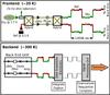 |
Fig. 1 Schematics of an LFI radiometer taken from Cal13. The two linearized polarization components are separated by an orthomode transducer (OMT), and each of them enters a twin radiometer, only one of which is shown in the figure. A first amplification stage is provided in the cold (20 K) focal plane, where the signal is combined with a reference signal originating in a thermally stable 4.5-K thermal load. The radio frequency signal is then propagated through a set of composite waveguides to the warm (300 K) backend, where it is further amplified and filtered, and finally converted into a sequence of digitized numbers by an analogue-to-digital converter. The numbers are then compressed into packets and sent to Earth. |
A schematic of the LFI pseudo-correlation receiver is shown in Fig. 1. We model the output voltage V(t) of each radiometer as  + M + N, \end{eqnarray}](/articles/aa/full_html/2016/10/aa26632-15/aa26632-15-eq9.png) (1)where G is the gain (measured in VK-1), B the beam response, D the thermodynamic temperature of the total CMB dipole signal (i.e., a combination of the solar and orbital components, including the quadrupolar relativistic corrections), which we use as a calibrator, and Tsky = TCMB + TGal + Tother is the overall temperature of the sky (CMB anisotropies, diffuse Galactic emission and other2 foregrounds, respectively) apart from D. Finally, M is a constant offset and N a noise term. In the following sections, we use Eq. (1) many times; whenever the presence of the N term is not important, it is silently dropped. The ∗ operator represents a convolution over the 4π sphere. We base our calibration on the knowledge of the spacecraft velocity around the Sun, which produces the orbital dipole, and use the orbital dipole to accurately measure the dominant solar dipole component. The purpose of this paper is to explain how we implemented and validated the pipeline that estimates the calibration constant K ≡ G-1 (which is used to convert the voltage V into a thermodynamic temperature), to quantify the quality of our estimate for K, and to quantify the impact of possible systematic calibration errors on the Planck/LFI data products.
(1)where G is the gain (measured in VK-1), B the beam response, D the thermodynamic temperature of the total CMB dipole signal (i.e., a combination of the solar and orbital components, including the quadrupolar relativistic corrections), which we use as a calibrator, and Tsky = TCMB + TGal + Tother is the overall temperature of the sky (CMB anisotropies, diffuse Galactic emission and other2 foregrounds, respectively) apart from D. Finally, M is a constant offset and N a noise term. In the following sections, we use Eq. (1) many times; whenever the presence of the N term is not important, it is silently dropped. The ∗ operator represents a convolution over the 4π sphere. We base our calibration on the knowledge of the spacecraft velocity around the Sun, which produces the orbital dipole, and use the orbital dipole to accurately measure the dominant solar dipole component. The purpose of this paper is to explain how we implemented and validated the pipeline that estimates the calibration constant K ≡ G-1 (which is used to convert the voltage V into a thermodynamic temperature), to quantify the quality of our estimate for K, and to quantify the impact of possible systematic calibration errors on the Planck/LFI data products.
Several improvements were introduced in the LFI pipeline for calibration relative to Cal13. In Sect. 2 we recall some terminology and basic ideas presented in Cal13 to discuss the normalization of the calibration, i.e., what factors influence the average value of G in Eq. (1). Section 3 provides an overview of the new LFI calibration pipeline and underlines the differences with the pipeline described in Cal13. One of the most important improvements in the 2015 calibration pipeline is the implementation of a new iterative algorithm to calibrate the data, DaCapo. Its principles are presented separately in a dedicated section, Sect. 4. This code has also been used to characterize the orbital dipole. The details of this latter analysis are provided in Sect. 5, where we present a new characterization of the solar dipole. These two steps are crucial for calibrating LFI. Section 6 describes a number of validation tests we have run on the calibration, as well as the results of a quality assessment. This section is divided into several parts: in Sect. 6.1 we compare the overall level of the calibration in the 2015 LFI maps with those in the previous data release; in Sect. 6.2 we provide a brief account of the simulations described in Planck Collaboration III (2016), which assess the calibration error due to the white noise and approximations in the calibration algorithm itself; in Sect. 6.3 we describe how uncertainties in the shape of the beams might affect the calibration; Sects. 6.4 and 6.5 measure the agreement between radiometers and groups of radiometers in the estimation of the TT power spectrum; and Sect. 6.6 provides a reference to the discussion of null tests provided in Planck Collaboration III (2016). Finally, in Sect. 7, we derive an independent estimate of the LFI calibration from our measurements of Jupiter and discuss its consistency with our nominal dipole calibration.
2. Handling beam efficiency
In this section we develop a mathematical model that relates the absolute level of the calibration (i.e., the average level of the raw power spectrum  for an LFI map) to a number of instrumental parameters related to the beams and the scanning strategy.
The beam response B(θ,ϕ) is a dimensionless function defined over the 4π sphere. In Eq. (1), B appears in the convolution 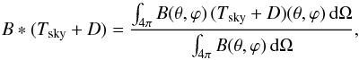 (2)whose value changes with time because of the change in orientation of the spacecraft. Since no time-dependent optical effects are evident from the data taken from October 2009 to February 2013 (Planck Collaboration IV 2016), we assume there is no intrinsic change in the shape of B during the surveys.
In the previous data release, we approximated B as a Dirac delta function (a pencil beam) when modelling the dipole signal seen by the LFI radiometers. The same assumption has been used for all the WMAP data releases (see, e.g., Hinshaw et al. 2009), as well as in the HFI pipeline (Planck Collaboration VIII 2016). However, the real shape of B deviates from the ideal case of a pencil beam because of two factors: (1) the main beam is more like a Gaussian with an elliptical section, whose FWHM (full width half maximum) ranges between 13′ and 33′ in the case of the LFI radiometers; and (2) farther than 5° from the beam axis, the presence of far sidelobes dilutes the signal measured through the main beam further and induces an axial asymmetry on B. Previous studies3 tackled the first point by applying a window function to the power spectrum computed from the maps to correct for the finite size of the main beam. However, the presence of far sidelobes might cause stripes in maps. For this 2015 data release, we used the full shape of B in computing the dipole signal adopted for the calibration. No significant variation in the level of the CMB power spectra with respect to the previous data release is expected, since we are basically subtracting power during the calibration process instead of reducing the level of the power spectrum by means of the window function. However, this new approach improves the internal consistency of the data, since the beam shape is taken into account from the very first stages of data processing (i.e., the signal measured by each radiometer is fitted with its own calibration signal Brad ∗ D); see Sect. 6.6. The definition of the beam window function has been changed accordingly; see Planck Collaboration IV (2016).
In Cal13 we introduced the two quantities φD and φsky as a way to quantify the impact of a beam window function on the calibration4 and on the mapmaking process, respectively. Here we briefly summarize the theory, and we introduce new equations that are relevant for understanding the normalization of the new Planck-LFI results in this data release.
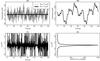 |
Fig. 2 Quantities used in determining the value of φsky (Eq. (8)) for radiometer LFI-27M (30 GHz) during a short time span (2 min). Panel A): the quantities Bmb ∗ TCMB and Bsl ∗ TCMB are compared. Fluctuations in the latter term are much smaller than those in the former. Panel B): the quantity Bsl ∗ TCMB shown in the previous panel is replotted here to highlight the features in its tiny fluctuations. That the pattern of fluctuations repeats twice depends on the scanning strategy of Planck, which observes the sky along the same circle many times with a spin rate of 1/60 Hz. Panel C): value of φsky calculated using Eq. (8). There are several values that diverge to infinity, which is due to the denominator in the equation going to zero. Panel D): distribution of the values of φsky plotted in panel C). The majority of the values fall around the number + 0.02%. |
Because of the motion of the solar system in the CMB rest frame, the solar dipole D is given by 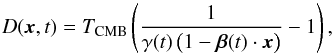 (3)where TCMB is the CMB monopole, β = v/c is the velocity of the spacecraft, and γ = (1−β2)− 1 / 2. Each radiometer measures the signal D convolved with the beam response B, according to Eq. (2); therefore, in principle, each radiometer has a different calibration signal. Under the assumption of a Dirac delta shape for B, Cal13 shows that the estimate of the gain constant
  is related to the true gain G by the formula
 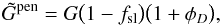 (4)where
 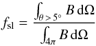 (5)is the fraction of power entering the sidelobes (i.e., along directions farther than 5° from the beam axis), and
 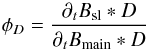 (6)is a time-dependent quantity that depends on the shape of B = Bmain + Bsl and its decomposition into a main (θ< 5°) and a sidelobe part, on signal D, and on the scanning strategy because of the time dependence of the stray light; the notation ∂t indicates a time derivative. Once the timelines are calibrated, traditional mapmaking algorithms approximate5B as a Dirac delta (e.g., Hinshaw et al. 2003; Jarosik et al. 2007; Keihänen et al. 2010), thus introducing a new systematic error. In this case, the mean temperature
  of a pixel in the map would be related to the true temperature Tsky by the formula
 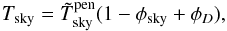 (7)which applies to timelines and should only be considered valid when considering details on angular scales larger than the width of the main beam. Cal13 defines the quantity φsky using the following equation:
 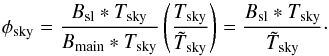 (8)See Fig. 2 for an example showing how φsky is computed.
In this 2015 Planck data release, we take advantage of our knowledge of the shape of B to compute the value of Eq. (2)and use this as our calibrator. Since the term B ∗ Tsky = (Bmain + Bsl) ∗ Tsky is unknown, we apply the following simplifications:
-
1.
we apply the point source and 80% Galactic masks (PlanckCollaboration 2015), in order not to consider theBmain ∗ Tsky term in the computation of the convolution;
-
2.
we assume that Bsl ∗ Tsky ≈ Bsl ∗ TGal and subtract it from the calibrated timelines, using an estimate for TGal computed by means of models of the Galactic emission (Planck Collaboration IX 2016; Planck Collaboration X 2016).
The result of such transformations is a new timeline  . Under the hypothesis of perfect knowledge of the beam B and of the dipole signal D, these steps are enough to estimate the true calibration constant without bias6 (unlike Eq. (4)):
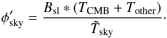
  (9)which should be expected, since no systematic effects caused by the shape of B affect the estimate of the gain G. To see how Eq. (7)changes in this case, we write the measured temperature as
  (10)Since in this 2015 data release we remove Bsl ∗ TGal, the contribution of the pickup of Galactic signal through the sidelobes (Planck Collaboration II 2016), the equation can be rewritten as
  (11)If we neglect details at angular scales smaller than the main beam size, then
 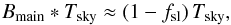 (12)so that
  (13)We modify Eq. (8)in order to introduce a new term
  :
:  (14)When solving for Tsky, Eq. (13)can be rewritten as
 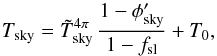 (15)where T0 = M/ (1−fsl) is a constant offset that is not very relevant for pseudo-differential instruments like LFI. Equation (15)is the equivalent of Eq. (7)in the case of a calibration pipeline that takes the 4π shape of B into account, as is the case for the Planck-LFI pipeline used for the 2015 data release.
Since one of the purposes of this paper is to provide a quantitative comparison of the calibration of this Planck data release with the previous one, we provide now a few formulae that quantify the change in the average level of the temperature fluctuations and of the power spectrum between the 2013 and 2015 releases. The variation in temperature can be derived from Eqs. (7)and (15): 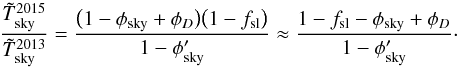 (16)If we consider the ratio between the power spectra
  and
and  , the quantity becomes
 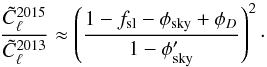 (17)In Sect. 6.1 we provide quantitative estimates of fsl, φD, φsky, and , as well as the ratios in Eqs. (16)and (17).
3. The calibration pipeline
In this section we briefly describe the implementation of the calibration pipeline. Readers interested in more detail should refer to Planck Collaboration II (2016).
Evaluating the calibration constant K (see Eq. (1)) requires us to fit the timelines of each radiometer with the expected signal D induced by the dipole as Planck scans the sky. This process provides the conversion between the voltages and the measured thermodynamic temperature.
As discussed in Sect. 2, we have improved the model used for D, since we are now computing the convolution of D with each beam B over the full 4π sphere. Moreover, we are considering the Bsl ∗ TGal term in the fit in order to reduce the bias due to the pickup of Galactic signal by the beam far sidelobes. The model of the dipole D now includes the correct7 quadrupolar corrections for special relativity. The quality of the beam estimate B has been improved as well: we are now using all seven Jupiter transits observed in the full four-year mission, and we account for the optical effects of the variation in the beam shape across the band of the radiometers. It is important to underline that these new beams do not follow the same normalization convention as in the first data release (now ∫4πB(θ,ϕ) dΩ ≠ 1) because numerical inaccuracies in the simulation of the 4π beams cause a loss of roughly 1% of the signal entering the sidelobes8: see Planck Collaboration IV (2016) for a discussion of this point.
As for the 2013 data release, the calibration constant K is estimated once per each pointing period, i.e., the period during which the spinning axis of the spacecraft holds still and the spacecraft rotates at a constant spinning rate of 1 / 60 Hz. The code used to estimate K, named DaCapo, has been completely rewritten; it is able to run in two modes, one of which (the so-called unconstrained mode) is able to produce an estimate of the solar dipole signal, and the other one (the constrained mode) which requires the solar dipole parameters as input. We used the unconstrained mode to assess the characteristics of the solar dipole, which were then used as input into the constrained mode of DaCapo for producing the actual calibration constants.
We smooth the calibration constants produced by DaCapo by means of a running mean, where the window size has a variable length. That length is chosen so that every time there is a sudden change in the state of the instrument (e.g., because of a change in the thermal environment of the front-end amplifiers) that discontinuity is not averaged out. However, this kind of filter removes any variation in the calibration constants, whose timescale is smaller than a few weeks. One example of this latter kind of fluctuation is the daily variation measured in the radiometer backend gains during the first survey, which was caused by the continuous turning on-and-off of the transponder9 while sending the scientific data to Earth once per day. To keep track of these fluctuations, we estimated the calibration constants K using the signal of the 4.5 K reference load in a manner similar to that described in Cal13 under the name of 4 K calibration, and we have added this estimate to the DaCapo gains after having applied a high-pass filter to them, as shown in Fig. 5. Details about the implementation of the smoothing filter are provided in Appendix A.
Once the smoothing filter has been applied to the calibration constants K, we multiply the voltages by K in order to convert them into thermodynamic temperatures and remove the term B ∗ D + Bsl ∗ Tsky from the result, thus removing the dipole and the Galactic signal captured by the far sidelobes from the data. The value for Tsky has been taken from a sum of the foreground signals considered in the simulations described in Planck Collaboration IX (2016); refer to Planck Collaboration II (2016) for further details.
4. The calibration algorithm
DaCapo is an implementation of the calibration algorithm we used in this data release to produce an estimate of the calibration constant K in Eq. (1). In this section we describe the model on which DaCapo is based, as well as a few details of its implementation.
4.1. Unconstrained algorithm
Let Vi be the ith sample of an uncalibrated data stream, and k(i) the pointing period to which the sample belongs. Following Eq. (1)and assuming the usual mapmaking convention of scanning the sky, Tsky, using a pencil beam, we model the uncalibrated time stream as  (18)where we write B ∗ Di ≡ (B ∗ D)i and use the shorthand notation Ti = (Tsky)i. The quantity Gk is the unknown gain factor for kth pointing period, ni represents white noise, and bk is an offset10 that captures the correlated noise component. We denote the sky signal by Ti , which includes foregrounds and the CMB sky apart from the dipole, and the dipole signal as seen by the beam B by B ∗ Di. The dipole includes both the solar and orbital components, and it is convolved with the full 4π beam. The beam convolution is carried out by an external code, and the result is provided as input to DaCapo.
The signal term is written with help of a pointing matrix P as  (19)Here P is a pointing matrix that picks the time-ordered signal from the unknown sky map m. The current implementation takes only the temperature component into consideration. In radiometer-based calibration, however, the polarization signal is partly accounted for, since the algorithm interprets whatever combination of the Stokes parameters (I,Q,U) the radiometer records as temperature signal. In regions that are scanned in only one polarization direction, this gives a consistent solution that does not induce any error on the gain. A small error can be expected to arise in those regions where the same sky pixel is scanned in vastly different directions of polarization sensitivity. The error is proportional to the ratio of the polarization signal and the total sky signal, including the dipole.
We determine the gains by minimizing the quantity  (20)where
 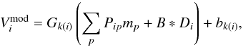 (21)and
  is the white noise variance. The unknowns of the model are m, G, b, and n (while we assume that the beam B is perfectly known). The dipole signal D and pointing matrix P are assumed to be known.
To reduce the uncertainty that arises from beam effects and subpixel variations in signal, we apply a galactic mask and include only those samples that fall outside the mask in the sum in Eq. (20).
Since Eq. (21)is quadratic in the unknowns, the minimization of χ2 requires iteration. To linearize the model, we first rearrange it as ![Mathematical equation: \begin{eqnarray} V_{i}^{\mathrm{mod}} &=& G_{k(i)}\left(B * D_{i}+\sum_{p}P_{ip}m_{p}^{0}\right) + G^{0}_{k(i)}\sum_{p}P_{ip} (m_{p}-m_{p}^{0}) \nonumber\\ && +\left[(G_{k(i)}-G^0_{k(i)})(m_{p}-m_{p}^{0}) \right] +b_{k(i)}. \end{eqnarray}](/articles/aa/full_html/2016/10/aa26632-15/aa26632-15-eq95.png) (22)Here G0 and m0 are the gains and the sky map from the previous iteration step. We drop the quadratic term in brackets and obtain
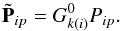
(22)Here G0 and m0 are the gains and the sky map from the previous iteration step. We drop the quadratic term in brackets and obtain 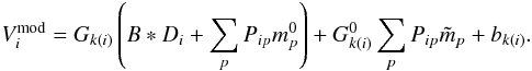 (23)Here
  (24)is a correction to the map estimate from the previous iteration step. Equation (23) is linear in the unknowns
  , G and b. We run an iterative procedure, where at each step we minimize χ2 with the linearized model in Eq. (23), update the map and the gains as
  and G0 → g, and repeat until convergence. The iteration is started from G0 = m0 = 0. Thus at the first step we are fitting just the dipole model and a baseline Gk(i)B ∗ Di + bk, and we obtain the first estimate for the gains. The first map estimate is obtained in the second iteration step.
DaCapo solves the gains for two radiometers of a horn at the same time. Two map options are available. Either the radiometers have their own sky maps, or both see the same sky. In the former case the calibrations become independent.
4.1.1. Solution of the linear system
Minimization of χ2 yields a large linear system. The number of unknowns is dominated by the number of pixels in map m. It is possible, however, to reformulate the problem as a much smaller system as follows.
We first rewrite the model using matrix notation. We combine the first and last terms of Eq. (23) formally into 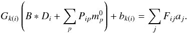 (25)The vector aj contains the unknowns b and G, and the matrix F spreads them into a time-ordered data stream. The dipole signal B ∗ D seen by the beam B, and a signal picked from map m0, are included in F.
Equation (21)can now be written in matrix notation as  (26)Gains G0 have been transferred inside matrix
  ,
,  (27)Using this notation, Eq. (20)becomes
  (28)where Cn is the white noise covariance.
Equation (28)is equivalent to the usual destriping problem of map-making (Planck Collaboration VI 2016), only the interpretation of the terms is slightly different. In place of the pointing matrix P we have , which contains the gains from the previous iteration step, and a contains the unknown gains beside the usual baseline offsets.
We minimize Eq. (28)with respect to  , insert the result back into Eq. (28), and minimize with respect to a. The solution is identical to the destriping solution
 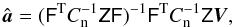 (29)where
 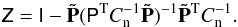 (30)We use a hat to indicate that
  is an estimate of the true a. We are here making use of the sparse structure of the pointing matrix, which allows us to invert matrix
  through non-iterative methods. For a detailed solution of an equivalent problem in mapmaking, see Keihänen et al. (2010) and references therein. The linear system in Eq. (29)is much smaller than the original one. The rank of the system is similar to the number of pointing periods, which is 44 070 for the full four-year mission.
Equation (29)can be solved by conjugate gradient iteration. The map correction is obtained as 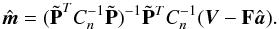 (31)Matrix
  is diagonal, and inverting it is a trivial task.
A lower limit for the gain uncertainty, based on radiometer white noise alone, is given by the covariance matrix 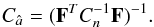 (32)
(32)
4.2. Constrained algorithm
4.2.1. Role of the solar dipole
The dipole signal is a sum of the solar and orbital contributions. The solar dipole can be thought of as being picked from an approximately11 constant dipole map, while the orbital component depends on beam orientation and satellite velocity. The latter can be used as an independent and absolute calibration. As we discuss in Sect. 5, this has allowed us to determine the amplitude and direction of the solar dipole and decouple the Planck absolute calibration from that of WMAP.
The solar dipole can be interpreted either as part of the dipole signal B ∗ D or part of the sky map m. This has important consequences. The advantage is that we can calibrate using only the orbital dipole, which is better known than the solar component and can be measured absolutely. (It only depends on the temperature of the CMB monopole and the velocity of the Planck spacecraft.) When the unconstrained DaCapo algorithm is run with erroneous dipole parameters, the difference between the input dipole and the true dipole simply leaks into the sky map m. The map can then be analysed to yield an estimate for the solar dipole parameters.
The drawback from the degeneracy is that the overall gain level is weakly constrained, since it is determined from the orbital dipole alone. In the absence of the orbital component, a constant scaling factor applied to the gains would be fully compensated for by an inverse scaling applied to the signal. It would then be impossible to determine the overall scaling of the gain. The orbital dipole breaks the degeneracy, but leaves the overall gain level weakly constrained compared with the relative gain fluctuations.
The degeneracy is not perfect, since the signal seen by a radiometer is modified by the beam response B. In particular, a beam sidelobe produces a strongly orientation-dependent signal. This is, however, a small correction to the full dipole signal.
4.2.2. Dipole constraint
Because of the degeneracy between the overall gain level and the map dipole, it makes sense to constrain the map dipole to zero. For this to work, two conditions must be fulfilled: 1) the solar dipole must be known; and 2) the contribution of foregrounds (outside the mask) to the dipole of the sky must either be negligible, or it must be known and included in the dipole model.
In the following we assume that both the orbital and the solar dipole are known. We aim at deriving a modified version of the DaCapo algorithm, where we impose the additional constraint  . Here mD is a a map representing the solar dipole component. We are thus requiring that the dipole in the direction of the solar dipole is completely included in the dipole model D, and nothing is left for the sky map. We note that mD only includes the pixels outside the mask.
It turns out that condition  alone is not sufficient, since there is another degeneracy in the model that must be taken into account. The monopole of the sky map is not constrained by data, since it cannot be distinguished from a global noise offset bk = const. It is therefore possible to satisfy the condition by adjusting the baselines and the monopole of the map simultaneously, with no cost in χ2. To avoid this pitfall, we simultaneously constrain the dipole and the monopole of the map. We require and 1Tm = 0, and combine them into one constraint
  (33)where mc now is a two-column object.
We add an additional prior term to Eq. (28)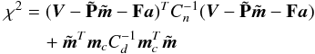 (34)and aim at taking
  to infinity. This will drive
  to zero.
Minimization of Eq. (34) yields the solution 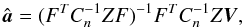 (35)with
  (36)where for brevity we have written
 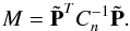 (37)This differs from the original solution (Eqs. (29), (30)) by the term
  in the definition of Z.
Equation (36)is impractical owing to the large size of the matrix to be inverted. To proceed, we apply the Sherman-Morrison formula and let CD → 0, yielding  (38)The middle matrix
  is a 2x2 block diagonal matrix, and is easy to invert.
Equations (35)−(38)are the basis of the constrained DaCapo algorithm. The system is solved using a conjugate-gradient method, similar to the unconstrained algorithm.
The map correction becomes  (39)One readily sees that
  fulfils the condition expressed by Eq. (33), and thus so does the full map m.
The constraint breaks the degeneracy between the gain and the signal, but also makes the gains again dependent on the solar dipole, which must be known beforehand.
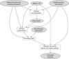 |
Fig. 3 Diagram of the pipeline used to produce the LFI frequency maps in the 2015 Planck data release. The grey ovals represent input/output data for the modules of the calibration pipeline, which are represented as white boxes. The product of the pipeline is a set of calibrated timelines that are passed as input to the mapmaker. |
4.3. Use of unconstrained and constrained algorithms
We have used the unconstrained and constrained versions of the algorithm together to obtain a self-consistent calibration and to obtain an independent estimate for the Solar dipole.
We first ran the unconstrained algorithm, using the known orbital dipole and an initial guess for the solar dipole. The results depend on the solar dipole only through the beam correction. The difference between the input dipole and the true dipole are absorbed in the sky map.
We estimated the solar dipole from these maps (Sect. 5); since the solar dipole is the same for all radiometers, we combined data from all the 70 GHz radiometers to reduce the error bars. (Simply running the unconstrained algorithm, fixing the dipole, and running the constrained version with same combination of radiometers would have just yielded the same solution.)
Once we had produced an estimate of the solar dipole, we reran DaCapo in constrained mode to determine the calibration coefficients K more accurately.
5. Characterization of the orbital and solar dipoles
In this section, we explain in detail how the solar dipole was obtained for use in the final DaCapo run mentioned above. We also compare the LFI measurements with the Planck nominal dipole parameters, and with the WMAP values given by Hinshaw et al. (2009).
5.1. Analysis
When running DaCapo in constrained mode to compute the calibration constants K (Eq. (1)), the code needs an estimate of the solar dipole in order to calibrate the data measured by the radiometers (see Sect. 3 and especially Fig. 3), since the signal produced by the orbital dipole is ten times weaker. We used DaCapo to produce this estimate from the signal produced by the orbital dipole. We limited our analysis to the 70 GHz radiometric data, since this is the cleanest frequency in terms of foregrounds. The pipeline was provided by a self-contained version of the DaCapo program, run in unconstrained mode (see Sect. 4.2), in order to make the orbital dipole the only source of calibration, while the solar dipole is left in the residual sky map.
We bin the uncalibrated differenced time-ordered data into separated rings, with one ring per pointing period. These data are then binned according to the direction and orientation of the beam, using a Healpix12 (Górski et al. 2005) map of resolution Nside = 1024 and 256 discrete bins for the orientation angle ψ. The far sidelobes should prevent a clean dipole from being reconstructed in the sky model map, since the signal in the timeline is convolved with the beam B over the full sphere. To avoid this, an estimate for the pure dipole is obtained by subtracting the contribution due to far sidelobes using an initial estimate of the solar dipole, which in this case was the WMAP dipole (Hinshaw et al. 2009). We also subtract the orbital dipole at this stage. The bias introduced by using a different dipole is of second order and is discussed in the section on error estimates (5.2).
DaCapo builds a model sky brightness distribution that is used to clean out the polarized component of the CMB and foreground signals to only leave noise, the orbital dipole, and far-sidelobe pickup. This sky map is assumed to be unpolarized, but since radiometers respond to a single linear polarization, the data will contain a polarized component, which is not compatible with the sky model and thus leads to a bias in the calibration. An estimate of the polarized signal, mostly CMB E modes and some synchrotron, needs to be subtracted from the timelines. To bootstrap the process we need an intial gain estimate, which is provided by DaCapo constrained to use the WMAP dipole. We then used the inverse of these gains to convert calibrated polarization maps from the previous LFI data release (which also used WMAP dipole calibration) into voltages and unwrap the map data into the timelines using the pointing information for position and boresight rotation. This polarized component due to E modes, which is ~ 3.5 μK rms on small angular scales plus an additional large-scale contribution of the North Galactic Spur of amplitude ~ 3 μK, was then subtracted from the time-ordered data. Further iterations using the cleaned timelines were found to make a negligible difference.
5.2. Results
To make maps of the dipole, a second DaCapo run was made in the unconstrained mode for each LFI 70 GHz detector using the polarization-cleaned timelines and the 30 GHz Madam mask, which allows 78% of the sky to be used. The extraction of the dipole parameters (Galactic latitude, longitude, and temperature amplitude) in the presence of foregrounds was achieved with a simple Markov chain Monte Carlo (MCMC) template-fitting scheme. Single detector hit maps, together with the white noise in the LFI-reduced instrument model (RIMO), were used to create the variance maps needed to construct the likelihood estimator for the MCMC samples. Commander maps (Planck Collaboration X 2016) were used for synchrotron, free-free, and thermal dust for the template maps with the MCMC fitting for the best amplitude scaling factor to clean the dipole maps. The marginalized distribution of the sample chains between the 16th and 84th percentiles were used to estimate the statistical errors, which were 0.̊004, 0.̊009, and 0.16μK for latitude, longitude, and amplitude respectively. The 50% point was taken as the best parameter value, as shown in Table 1. To estimate the systematic errors on the amplitude in calibration process due to white noise, 1 /f noise, gain fluctuations, and ADC corrections, simulated time-ordered data were generated with these systematic effects included. These simulated timelines were then calibrated by DaCapo in the same way as the data. The standard deviation of the input to output gains were taken as the error in absolute calibration with an average value of 0.11%.
Plots of the dipole amplitudes with these errors are shown in Fig. 6, together with the error ellipses for the dipole direction. As can be seen, the scatter is greater than the statistical error. Therefore, we take a conservative limit by marginalizing over all the MCMC samples for all the detectors, which results in an error ellipse (±0.̊02, ±0.̊05) centred on Galactic latitude and longitude (48.̊26, 264.̊01). The dipole amplitudes exhibit a trend in focal plane position, which is likely due to residual, unaccounted-for power in far sidelobes, which would be symmetrical between horn pairs. These residuals, interacting with the solar dipole, would behave like an orbital dipole, but in opposite ways on either side of the focal plane. This residual therefore cancels out to first order in each pair of symmetric horns in the focal plane, i.e., horns 18 with 23, 19 with 22, and 20 with 21 (see inset in Fig. 6). Since the overall dipole at 70 GHz is calculated by combining all the horns, the residual effect of far sidelobes is reduced.
Dipole characterization from 70 GHz radiometers.
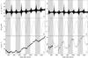 |
Fig. 4 Variation in time of a few quantities relevant for calibration for radiometers LFI-21M (70 GHz, left) and LFI-27M (30 GHz, right). Grey/white bands indicatecomplete sky surveys. All temperatures are thermodynamic. Panel A): calibration constant K estimated using the expected amplitude of the CMB dipole. The uncertainty associated with the estimate changes with time, according to the amplitude of the dipole as seen in each ring. Panel B): expected peak-to-peak difference in the dipole signal (solar + orbital). The shape of the curve depends on the scanning strategy of Planck, and it is strongly correlated with the uncertainty in the gain constant (see panel A)). The deepest minima happen during Surveys 2 and 4; because of the higher uncertainties in the calibration (and the consequent bias in the maps), these surveys have been neglected in some of the analyses in this Planck data release (see, e.g., Planck Collaboration XIII 2016). Panel C): the calibration constants K used to actually calibrate the data for this Planck data release are derived by applying a smoothing filter to the raw gains in panel A). Details regarding the smoothing filter are presented in Appendix A. |
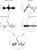 |
Fig. 5 Visual representation of the algorithms used to filter the calibration constants produced by DaCapo (top left plot; see Sect. 4). The example in the figure refers to radiometer LFI-27M (30 GHz) and only shows the first part of the data (roughly three surveys). |
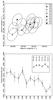 |
Fig. 6 Dipole amplitudes and directions for different radiometers. Top: errors in the estimation of the solar dipole direction are represented as ellipses. Bottom: estimates of the amplitude of the solar dipole signal; the errors here are dominated by gain uncertainties. Inset: the linear trend (recalling that the numbering of horns is approximately from left to right in the focal plane with respect to the scan direction), most likely caused by a slight symmetric sidelobe residual, is removed when we pair the 70 GHz horns. |
6. Validation of the calibration and accuracy assessment
Accuracy in the calibration of LFI data.
In this section we present the results of a set of checks we have run on the data that comprise this new Planck release. Table 2 quantifies the uncertainties that affect the calibration of the LFI radiometers.
6.1. Absolute calibration
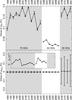 |
Fig. 7 Top: estimate of the value of φD (Eq. (6)) for each LFI radiometer during the whole mission. The plot shows the median value of φD over all the samples and the 25th and 75th percentiles (upper and lower bar). These bars provide an idea of the range of variability of the quantity during the mission; they are not an error estimate of the quantity itself. Bottom: estimate of the value of φsky (Eq. (8)). The points and bars have the same meaning as in the plot above. Because of the low value for the 44 and 70 GHz channels, the inset shows a zoom of their median values. The large bars for the 30 GHz channels are motivated by the coupling between the stronger foregrounds and the relatively large power falling in the sidelobes. |
Optical parametersa of the 22 LFI beams.
In this section we provide an assessment of the change in the absolute level of the calibration since the first Planck data release, in terms of its impact on the maps and power spectra. Generally speaking, a change in the average value of G in Eq. (1)of the form  (40)leads to a change of ⟨T⟩ → ⟨T⟩(1 + δG) in the average value of the pixel temperature T, and to a change Cℓ → Cℓ(1 + 2δG) in the average level of the measured power spectrum Cℓ, before the application of any window function. Our aim is to quantify the value of the variation δG from the previous Planck-LFI data release to the current one. We did this by comparing the level of power spectra in the ℓ = 100–250 multipole range consistently with Cal13.
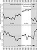 |
Fig. 8 Top: comparison between the measured and estimated ratios of the aℓm harmonic coefficients for the nominal maps (produced using the full knowledge of the beam B over the 4π sphere) and the maps produced under the assumption of a pencil beam. The estimate has been computed using Eq. (11). Bottom: difference between the measured ratio and the estimate. The agreement is better than 0.03% for all 22 LFI radiometers. |
There have been several improvements in the calibration pipeline that have led to a change in the value of ⟨G⟩:
-
1.
The peak-to-peak temperature difference of the referencedipole D used in Eq. (1)has changed by + 0.27% (see Sect. 5), because we now use the solar dipole parameters calculated from our own Planck measurements (Planck Collaboration I 2016).
-
2.
In the same equation, we no longer convolve the dipole D with a beam B that is a delta function, but instead use the full profile of the beam over the sphere (see Sect. 2).
-
3.
The beam normalization has changed, since in this data release B is such that (Planck Collaboration IV 2016)
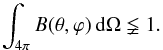 (41)
(41) -
4.
The old dipole fitting code has been replaced with a more robust algorithm, DaCapo (see Sect. 4).
Table 4 lists the impact of these effects on the amplitude of fluctuations in the temperature ⟨T⟩ of the 22 LFI radiometer maps. The numbers in this table have been computed by rerunning the calibration pipeline on all the 22 LFI radiometer data with the following setup:
-
1.
A pencil-beam approximation for B in Eq. (1)has been used, instead of the full 4π convolution (“Beam convolution” column), with the impact of this change quantified by Eq. (16), and the comparison between the values predicted by this equation with the measured change in the aℓm harmonic coefficients shown in Fig. 8 (the agreement is excellent, better than 0.03%).
-
2.
The old calibration code has been used instead of the DaCapo algorithm described in Sect. 4 (“Pipeline upgrades” column).
-
3.
The B ∗ TGal term has not been removed, as in the discussion surrounding Eq. (11)(“Galactic sidelobe removal” column).
-
4.
The signal D used in Eq. (1)has been modelled using the dipole parameters published in Hinshaw et al. (2009), as was done in Cal13 (“Reference dipole” column).
We measured the actual change in the absolute calibration level by considering the radiometric maps (i.e., maps produced using data from one radiometer) of this data release (indicated with a prime) and of the previous data release and averaging the ratio: 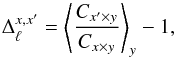 (42)where y indicates a radiometer at the same frequency as x and x′, such that y ≠ x. The average is meant to be taken over all the possible choices for y (thus 11 choices for 70 GHz radiometers, 5 for 44 GHz, and 3 for 30 GHz) in the multipole range 100 ≤ ℓ ≤ 250. The way that cross-spectra are used in Eq. (42)ensures that the result does not depend on the white noise level. Of course, this result quantifies the ratio between the temperature fluctuations (more correctly, between the aℓm coefficients of the expansion of the temperature map in spherical harmonics) in the two data releases, and not between the power spectra.
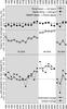 |
Fig. 9 Top: impact on the average value of the aℓm spherical harmonic coefficients (computed using Eq. (42), with 100 ≤ ℓ ≤ 250) because of several improvements in the LFI calibration pipeline, from the first to the second data release. Bottom: measured change in the aℓm harmonic coefficients between the first and the second data releases. No beam window function has been applied. These values are compared with the estimates produced using Eq. (43), which assumes perfect independence among the effects. |
The column labelled “Estimated change” in Table 4 contains a simple combination of allthe numbers in the table:  (43)where the ϵ factors are the numbers shown in the same table and discussed above. This formula assumes that all the effects are mutually independent. This is, of course, an approximation; however, the comparison between this estimate and the measured value (obtained by applying Eq. (42) to the 2013 and 2015 release maps) can give an idea of the amount of interplay of these effects in producing the observed shift in temperature. Figure 9 shows a plot of the contributions discussed above, as well as a visual comparison between the measured change in the temperature and the estimate from Eq. (43).
6.2. Noise in dipole fitting
We performed a number of simulations that quantify the impact of white noise in the data on the estimation of the calibration constant, as well as the ability of our calibration code to retrieve the true value of the calibration constants. Details of this analysis are described in Planck Collaboration III (2016). We did not include such sorts of errors as an additional element in Table 2, because the statistical error is already included in the row “Spread among independent radiometers”.
Changes in the calibration level between this (2015) Planck-LFI data release and the previous (2013) one.
6.3. Beam uncertainties
As discussed in Planck Collaboration IV (2016), the beams B used in the LFI pipeline are very similar to those presented in Planck Collaboration IV (2014); they are computed with GRASP, properly smeared to take the satellite motion into account. Simulations were performed using the optical model described in Planck Collaboration IV (2014), which was derived from the Planck radio frequency Flight Model (Tauber et al. 2010) by varying some optical parameters within the nominal tolerances expected from the thermoelastic model, in order to reproduce the measurements of the LFI main beams from seven Jupiter transits. This is the same procedure adopted in the 2013 release (Planck Collaboration IV 2014); however, unlike the case presented in Planck Collaboration IV (2014), a different beam normalization is introduced here to properly take the actual power entering the main beam into account (typically about 99% of the total power). This is discussed in more detail in Planck Collaboration IV (2016).
Given the broad use of beam shapes B in the current LFI calibration pipeline, it is extremely important to assess their accuracy and the way errors in B propagate down to the estimate of the calibration constants K in Eq. (1).
In the previous data release we did not use our knowledge of the bandpasses of each radiometer to produce an in-band model of the beam shape, but instead estimated B by means of a monochromatic approximation (see Cal13). In that case, we estimated the error induced in the calibration as the variation of the dipole signal when using either a monochromatic or a band-integrated beam, since we believe the latter to be a more realistic model.
In this data release, we have switched to the full bandpass-integrated beams produced using GRASP, which represents our best knowledge of the beam (Planck Collaboration IV 2016). We tested the ability of DaCapo to retrieve the correct calibration constants K for LFI19M (a 70 GHz radiometer) when the large-scale component (ℓ = 1) of the beam’s sidelobes is: (1) rotated arbitrarily by an angle −160° ≤ θ ≤ 160°; or (2) scaled by ± 20%. We find that such variations alter the calibration constants by approximately 0.1%. However, we do not list such a small number as an additional source of uncertainty in Table 2, since we believe that this is already captured by the scatter in the points shown in Fig. 10, which were used to produce the numbers in the row Inconsistencies among radiometers.
6.4. Inter-channel calibration consistency
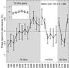 |
Fig. 10 Discrepancy among the radiometers of the same frequency in the height of the power spectrum Cℓ near the first peak. For a discussion of how these values were computed, see the text. Inset: to better understand the linear trend in the 70 GHz radiometers, we have computed the weighted average between pairs of radiometers whose position in the focal plane is symmetric. The six points refer to the combinations 18M/23M, 18S/23S, 19M/22M, 19S/22S, 20M/21M, and 20S/21S, respectively. All six points are consistent with zero within 1σ; see also Fig. 6. |
In this section we provide a quantitative estimate of the relative calibration error for the LFI frequency maps by measuring the consistency of the power spectra computed using data from one radiometer at time. By relative error we mean any error that is different among the radiometers, in contrast to an absolute error, which induces a common shift in the power spectrum. We computed the power spectrum of single radiometer half-ring maps and have estimated the variation in the region around the first peak (100 ≤ ℓ ≤ 250), since this is the multipole range with the best S/N.
The result of this analysis is shown in Fig. 10, which plots the values of the quantity  (44)where
  is the cross-power spectrum computed using two half-ring maps, and ⟨·⟩ denotes an average over ℓ. The quantity ⟨Cℓ⟩freq is the same average computed using the full frequency half-ring maps. The δrad slope is symmetric around zero in the 70 GHz radiometers; this might be caused by residual unaccounted-for power in the far sidelobes of the beam. The same explanation was advanced in Sect. 5 to explain a similar effect. It is interesting to note that the amplitude of the two systematics is comparable; the trend in Fig. 6 has a peak-to-peak variation (in temperature) of about 0.5%, while the trend in Fig. 10 has a variation (in power) of roughly 1.0%. We combine the values of δrad for those pairs of radiometers whose beam position in the focal plane is symmetric (e.g., 18M versus 23M, 18S versus 23S, 19M versus 22M, etc.), since in these pairs the unaccounted-for power should be balanced. We have found that indeed all the six combinations of δrad are consistent with zero within 1 σ (see the inset of Fig. 10).
Since the cross-spectrum of two half-ring maps does not depend on the level of uncorrelated noise, the fluctuations of δi around the average value that can be seen in Fig. 10 can be interpreted as relative calibration errors. If we limit our analysis to the multipole range 100 ≤ ℓ ≤ 250, we can estimate the error of the 70 GHz map as the error on the average height of the peaks (i.e., the value  , with σ being the standard deviation and N the number of points) that is, 0.25, 0.16, and 0.10 percent and 30, 44, and 70 GHz, respectively.
6.5. Inter-frequency calibration consistency
In this section we carry out an analysis similar to the one presented in Sect. 6.4, where we compare the absolute level of the maps at the three LFI frequencies, i.e., 30, 44, and 70 GHz. We make use of the full frequency maps, as well as the pair of half-ring maps at 70 GHz. Each half-ring map has been produced using data from one of the two halves of each pointing period. We quantify the discrepancy between the 70 GHz map and another map by means of the quantity 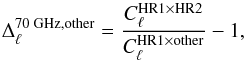 (45)where
  is the cross-spectrum between the two 70 GHz half-ring maps, and
  is the cross-spectrum between the first 70 GHz half-ring map and the map under analysis. In the ideal case (perfect correspondence between the spectrum of the 70 GHz map and the other map) we expect Δℓ = 0. As was the case for Eq. (44), this formula has the advantage of discarding the white noise level of the spectrum
  by using the cross-spectrum with the 70 GHz map, whose noise should be uncorrelated.
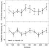 |
Fig. 11 Estimate of |

Over the multipole range 100 ≤ ℓ ≤ 250, the average discrepancy13 is 0.15 ± 0.17% for the 44 GHz map, and 0.15 ± 0.26% for the 30 GHz map, as shown in Fig. 11. Such numbers are consistent with the calibration errors provided in Sect. 6.4.
Visibility epochs of Jupiter.
6.6. Null tests
In Cal13 we provided a study of a number of null tests, with the purpose of testing the quality of the calibration. In this new data release, we have moved the bulk of the discussion to Planck Collaboration III (2016). We just show one example here, which is particularly relevant in the context of the LFI calibration validation. Figure 12 shows the variation in the quality of the maps due to the use of the full 4π convolution versus a pencil beam approximation, as discussed in Sect. 2. The analysis of many similar difference maps has provided us with sufficient evidence that using the full 4π beam convolution reduces the level of systematic effects in the LFI maps.
7. Measuring the brightness temperature of Jupiter
The analysis of the flux densities of planets for this Planck data release has been considerably extended. We only use Jupiter data for planet calibration, so we now focus the discussion on observations of this planet. The new analysis includes all seven transits of Jupiter through each main beam of the 22 LFI radiometers. The analysis pipeline has been improved considerably by considering several effects not included in Cal13.
Planets provide a useful calibration cross-check; in particular, the measurement of the brightness temperature of Jupiter can be a good way to assess the accuracy of the calibration, since Jupiter is a remarkably bright source with a S/N per scan as high as 50 and a relatively well known spectrum. Furthermore, at the resolution of LFI beams, it can be considered a point-like source.
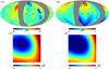 |
Fig. 12 Difference in the application of the full 4π beam model versus the pencil beam approximation. Panel A): difference between survey 1 and survey 2 for a 30 GHz radiometer (LFI-27S) with the 4π model, smoothed to 15°. We do not show the same difference with pencil beam approximation, because it would appear indistinguishable from the 4π map. Panel B): double difference between the 4π1-2 survey difference map in panel A and the pencil difference map (not shown here). This map shows what changes when one drops the pencil approximation and uses the full shape of the beam in the calibration. Panel C): zoom on the blue spot visible at the top of the map in panel A). Panel D): same zoom for the pencil approximation map. The comparison between panels C) and D) shows that the 4π calibration produces better results. |
 |
Fig. 13 Visual timeline of Jupiters’s crossings with LFI beams. Here SS lables sky surveys. |
 |
Fig. 14 Time dependence of the angle between Jupiter’s direction and the spin axis of the Planck spacecraft. The darker horizontal bar indicates the angular region of the 11 LFI beam axes, and the lighter bar is enlarged by ± 5°. |
7.1. Input data
Table 5 lists the epochs when the LFI main beams crossed Jupiter, and Figs. 13 and 14 give a visual timeline of these events. The first four transits occurred in nominal scan mode (spin shift 2′, 1° per day) with a phase angle of 340°, and the last three scans in deep mode (shift of the spin axis between rings of 0.5′, 15′ per day) with a phase angle of 250° (see Planck Collaboration I 2016). The analysis follows the procedure outlined in Cal13, but with a number of improvements:
-
1.
The brightness of Jupiter was extracted from timelines to fullyexploit the time dependence in the data.
-
2.
Seven transits have been considered instead of two, which allowed us to analyse the sources of scatter better among the measurements.
-
3.
All the data were calibrated simultaneously.
-
4.
Different extraction methods were exploited to find the most reliable among them.
In the following discussion, we refer to a timeline (one for each of the 22 LFI radiometers) as the list of values (t,xp,t,xt,ψt,ΔTant,t) with t the epoch of observation, xp,t the instantaneous apparent planet positions as seen from Planck, xt and ψt the corresponding beam pointing directions and orientations, and ΔTant,t the measured antenna temperature. We took the the values of xt and ψt, as well as the calibrated values of ΔTant,t cleaned from the dipole and quadrupole signals, from the output of the LFI pipeline. We recovered xp,t from the Horizons14 on-line service.
Samples from each radiometer timeline were used in this analysis only if the following conditions were met: (1) the samples were acquired in stable conditions during a pointing period (Planck Collaboration II 2016); (2) the pipeline did not flag them as “bad”; (3) their angular distance from the planet position at the time of the measurement was less than 5°; and (4) they were not affected by any anomaly or relevant background source. We checked the last condition by visually inspecting small coadded maps of the selected samples.
7.2. Description of the analysis pipeline
In the following paragraphs, we describe how we improved the pipeline used to extract the brightness temperature TB of Jupiter from the raw LFI data. This extraction goes through an initial estimation of the antenna temperature TA and a number of corrections to take various systematic effects into account. We present the methods used to estimate TA in Sect. 7.2.1, and then in Sect. 7.2.2 we discuss the estimation of TB. Since the computation of TB requires an accurate estimate of the planet solid angle Ωp, we discuss the computation of this factor in a dedicated part, Sect. 7.2.3.
7.2.1. Estimation of the antenna temperature
Following Cal13 and Cremonese et al. (2002), the recovery of the instantaneous planet signal from a timeline is equivalent to the deconvolution of the planet shape from the beam pattern Bt at time t. Since the planet can be considered a point source, the most practical way is to assume  (46)where TA,p is the unknown planet antenna temperature, b the background, and Bt(δxp,t) the beam response for the planet at the time of observation. Of course, Bt depends on the relative position of the planet with respect to the beam, δxp,t. If a suitable beam model is available, Bt can be determined and TA,p can be recovered from least squares minimization. We use an elliptic Gaussian centred on the instantaneous pointing direction as a model for the beam, because it shows a very good match with the main beam of the GRASP model (Planck Collaboration IV 2016), with peak-to-peak discrepancies of a few tenths of a percent (the importance of far sidelobes is negligible for a source as strong as Jupiter). To compute Bt, the pointings are rotated into the beam reference frame, since this allows for better control of the beam pattern reconstruction15.
7.2.2. Estimation of the brightness temperature
In Cal13, we computed the brightness temperature TB from the antenna temperature TA by means of the following formula (assuming monochromatic radiometers):  (47)where BPlanck is Planck’s blackbody function, Ωb and Ωp the beam and planet solid angles, and TCMB = 2.7255 K is the temperature of the CMB monopole. In this 2015 Planck data release, we have also introduced corrections to account for the bandpass.
The accuracy of the TB determination is affected by confusion noise (i.e., noise caused by other structures in the maps), which we estimate from the standard deviation of samples taken between a radius of 1° and 1.5° (depending on the beam) and 5° from the beam centre. These samples are masked for strong sources or other defects. Since background maps are not subtracted, the confusion noise is greater than the pure instrumental noise. However, since the histogram is described well by a normal distribution, we used error propagation16 to assess the accuracy of TB against the confusion noise.
In the conversion of TA,p into TB through Eq. (46), the pipeline implements a number of small corrections:
-
1.
detector-to-detector differences in the beam solid angleΩb, accounting for ± 6%, which is probably the most important effect;
-
2.
changes in the solid angle of the planet, Ωp, due to the change of the Jupiter–Planck distance, which introduces a correction factor of up to 6.9% percent;
-
3.
changes in the projected planet ellipticity, due to the planeto-centric latitude of the observer and the oblateness of the planet, to reduce observations as if they were made at Jupiter’s pole;
-
4.
blocking of background radiation by the planet, changing from about 0.7% to 1.5%, depending on the ratio Ωp/ Ωb;
-
5.
a φsl correction, which accounts for the fraction of radiation not included in the main beam (about 0.2%).
7.2.3. Determination of the solid angle of Jupiter
The solid angle Ωp of Jupiter for a given planet-spacecraft distance Δp and planeto-centric latitude δP is given by  (48)where Δp,ref is a fiducial planet-spacecraft distance (for Jupiter, Δp,ref ≈ 5.2 AU),
  is the solid angle of the planet as seen from its pole at the fiducial distance, and ep(< 1) the ratio between the polar and equatorial radii of the planet.
Our new pipeline does not use the ellipticity, FWHM, and orientation of the elliptical beam parameters provided by Planck Collaboration IV (2016), as they were derived from a marginalization over TA,p on the same Jupiter data used in this analysis. However, because of a degeneracy between TA,p and the beam parameters, the results were sensitive to details of the fitting procedure (up to about 1%), such as the radius of the area being analysed and the minimization method. Therefore, we have first determined a new set of beam parameters for each transit and computed the weighted average (using a numerical minimization), and then we used these parameters to determine TA,p.
7.3. Results
We present here the results per radiometer and transit, and we also discuss how to combine the measurements performed using the 30, 44, and 70 GHz radiometers to obtain three estimates of TB at these three nominal frequencies.
7.3.1. Brightness temperatures per radiometer and transit
In Cal13, based on the first two transits, we noted that confusion noise alone was not able to account for variations in TB found for different radiometers belonging to the same frequency channel. We therefore assumed the presence of some unidentified systematics error, dominating the ultimate accuracy in the measures.
That residual systematics are more important than confusion noise and background is still true in the 2015 data release. The values of TB measured by radiometers in the same frequency channel have a spread of 0.6%, 1.0%, and 0.6% of the average signal at 30, 44 and 70 GHz, respectively, and are not normally distributed (see Fig 15). These observed dispersions are a factor of ~ 3 larger than the confusion noise, and cannot be ascribed to the background, whose effect is only 1% of the observed scatter. The excess dispersion must be due to a small residual systematic effect such as pointing, beam model, or mismatch in the centre frequency.
One possible cause of the observed dispersion in the brightness temperature is some systematic effect in the estimation of the beam parameters (see Sect. 7.2.3).
Non-Gaussianities in the beam, as well as beam smearing were investigated by replacing the elliptical beam with band-averaged beam maps derived from GRASP calculations. The results are consistent with the elliptical beam, with residuals of at most 4 × 10⁻³ K in TA,p.
We computed TA,p and TB again using an analytical approximation based on the assumption of negligible background (which is quite a good approximation for Jupiter), and compared the results. The two methods agree at the level of 6 × 10⁻⁷ K for TA,p, and at the level of 6 × 10⁻⁴ K for TB.
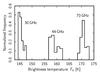 |
Fig. 15 Distribution of the values of TB for Jupiter measured by the 22 LFI radiometers during each of the seven transits. The histogram has been produced using five bins per frequency. The lack of Gaussianity in the three distributions is evident. |
7.3.2. Combination of the results and comparison with WMAP
We now want to combine the measurements of the 22 LFI radiometers in order to have three estimates of TB at the three LFI nominal frequencies, 30, 44, and 70 GHz.
Such a determination of TB depends on proper knowledge of the central frequency, νcen, for each detector. This parameter is derived from the bandpasses, but these are not known exactly. It is possible to remove most of the differences amongst the 30 GHz and amongst the 44 GHz radiometers by changing the νcen values of the radiometers by as little as ± 0.2 GHz. However, it is still not clear how the bandshapes would have to be modified to explain these changes in νcen. For this reason, we did not include these corrections for 30 GHz and 44 GHz data.
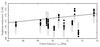 |
Fig. 16 Distribution of the values of Tb for Jupiter as a function of the central frequency νcen of each radiometer. |
At 70 GHz the situation is complicated even more by the fact that the νcen values of the radiometers are significantly spread over the channel bandwidth, so that each of the 70 GHz radiometers samples a slightly different portion of the Jupiter spectrum. Indeed, comparing TB at 70 GHz from one transit to the next after having ordered the radiometers for increasing νcen, it is possible to see quite a significant correlation (see Fig. 16). Using a linear regression of the TB at 70 GHz against νcen, a cleaned list of TB values was obtained. Their average is identical to the simple weighted average of TB for all of the transits and of the detectors TB = (171.558 ± 0.008) K. The standard deviation of the whole set of samples reduces to just 2.7%. Interestingly, the inferred slope dTB/ dνcen = (0.2570 ± 0.0058) K / GHz matches the one from WMAP data very well, dTB/ dνcen = (0.243 ± 0.025) K / GHz, and the correlation between transits loses most of its statistical significance. We attempted the same test for the 30 GHz and 44 GHz channels, but the spread in νcen is too small to produce meaningful results. These results open the possibility of including the spectral slope directly as a free parameter of the fit in a future analysis.
Brightness temperature of Jupiter.
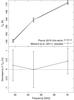 |
Fig. 17 Top: brightness temperature of Jupiter (Tbr) compared with the data from Weiland et al. (2011), linearly rescaled in frequency to match LFI’s central frequencies νcen and corrected for difference between the LFI and WMAP dipoles. Bottom: deviation from unity of the ratio between LFI’s estimate for Tbr and WMAP’s. The agreement is excellent among the three frequencies. |
The result of this analysis produced the brightness temperatures TB listed in Table 6. The errors are 0.6%, 0.9%, and 0.6% at 30, 44, and 70 GHz, respectively. As in Cal13, in Fig. 17 we compared Jupiter’s TB averaged in each LFI band with the spectrum provided by WMAP. The agreement is quite good, with a difference that does not exceed 0.5%. In this comparison, we must note that WMAP and Planck-LFI are calibrated on slightly different dipoles, with Planck assuming an amplitude of 3364.5 μK (Planck Collaboration I 2016), while WMAP assumed an amplitude of 3355 μK (Hinshaw et al. 2009). In addition, WMAP central frequencies are different from those of Planck. So to make the comparison, the measures provided in Weiland et al. (2011) are scaled by 1.00268 and linearly interpolated to the averaged νcen of each LFI frequency channel.
7.4. What does the analysis of Jupiter tell about the LFI calibration?
The errors in our estimates of Jupiter’s brightness temperature are 0.6%, 0.9%, and 0.6%. These are consistent with (albeit slightly larger than) the numbers presented in Sects. 6.4 and 6.5, where our analysis of the consistency of inter-channel and inter-frequency cross-spectra in the range 100 ≤ ℓ ≤ 250 produced estimates between 0.1% and 0.3%. We believe that the larger error bars are a direct consequence of a number of facts: (1) bandpass uncertainties play a larger role in the analysis of a non-thermodynamic sky signal like Jupiter’s emission in the microwave range; (2) the amount of data usable for this analysis is only a limited fraction of the overall amount used to create LFI maps; and (3) uncertainties in the main beam profile have a larger impact on the study of a point-like source such as Jupiter, with respect to the analysis presented in Sect. 6, which dealt with angular scales corresponding to 100 ≤ ℓ ≤ 250.
8. Conclusions
We have described the method used to calibrate the Planck/LFI data for the 2015 Planck data release and provided a quantitative analysis that shows the amount of change in detail at the calibration level thanks to all the improvements we implemented in the pipeline since the previous data release. Compared to our 2013 release, we have improved the LFI calibration in several ways, most notably in the use of an internally consistent dipole signal as a calibrator, as well as more accurate data analysis algorithms. As a result, we have also improved the accuracy of the LFI calibration by a factor of 3, which for the 2015 release ranges from 0.20% to 0.35%, depending on the frequency.
An important byproduct of our analysis is a novel estimate of the solar dipole signal; using LFI data alone, we have estimated the amplitude of the dipole to be 3 365.6 ± 3.0 μK and the direction of its axis to be (l,90°−b) = (264.01 ± 0.05°,48.26 ± 0.02°) (Galactic coordinates). This result matches the numbers provided by Hinshaw et al. (2009) within 1σ. This slight difference in amplitude has the effect of a shift by ~ 0.3% in the overall level of the calibrated timelines. Together with the improved LFI calibration, we now find very good agreement between the level of the spectra estimated by WMAP.
Planck (http://www.esa.int/Planck) is a project of the European Space Agency (ESA) with instruments provided by two scientific consortia funded by ESA member states and led by Principal Investigators from France and Italy, telescope reflectors provided through a collaboration between ESA and a scientific consortium led and funded by Denmark, and additional contributions from NASA (USA).
Within this term we include extragalactic foregrounds and all point sources.
Apart from the use of appropriate window functions (e.g., Page et al. 2003), the WMAP team implemented a number of other corrections to further reduce systematic errors due to the non-ideality of their beams. In their first data release, the WMAP team estimated the contribution of the Galaxy signal picked up through the sidelobes at the map level (Barnes et al. 2003) and then subtracted them from the maps. Starting from the third year release, they estimated a multiplicative correction, called the recalibration factor, assumed constant throughout the survey, by means of simulations. This constant accounts for the sidelobe pickup and has been applied to the TODs (Jarosik et al. 2007). The deviation from unity of this factor ranges from 0.1% to 1.5%.
The definition of φD provided in Cal13 was not LFI-specific: it can be applied to any experiment that uses the dipole signal for the calibration.
Keihanen & Reinecke (2012) provide a deconvolution code that can be used to produce maps potentially free of this effect.
Because of a bug in implementing the pipeline, the previous data release had a spurious factor that led to a residual quadrupolar signal of ~ 1.9 μK, as described in Cal13.
This loss was present in the beams used for the 2013 release too, but in that case we applied a normalization factor to B. We removed this normalization because it had the disadvantage of uniformly spreading the 1% sidelobe loss over the whole 4π sphere.
This operating mode was subsequently changed, and the transponder has been kept on for the remainder of the mission starting from 272 days after launch, thus removing the origin of this kind of gain fluctuations.
The offset absorbs noise at frequencies lower than the inverse of the pointing period length (typically 40 min). The process of coadding scanning rings efficiently reduces noise at higher frequencies. We treat the remaining noise as white.
It is not exactly constant, since the dipole signal is B ∗ D. Since the orientation of B changes with time, any deviation from axial symmetry in B (ellipticity, far sidelobes, etc.) falsifies this assumption. However, when convolving a large-scale signal such as the CMB dipole with the LFI beams, such asymmetries are a second-order effect.
To reduce the impact of the Galactic signal we have masked 60% of the sky, since we found that less aggressive masks produced significant biases in the ratios.
This is the opposite of Cal13, which used the planet reference frame.
We can quickly derive an order of magnitude for the size of the confusion noise effect in the estimation of TA. Since the confusion noise is of the order of a few mK and the number N of samples within 2 FWHM (the radius used for estimating TB) is of the order of 103–104, we can expect an accuracy of the order of  .
.
The null tests we used in this process are typically the difference between survey maps; in the case of an ideal, perfectly calibrated instrument, such differences should yield a map where all the pixels are zero.
Acknowledgments
The Planck Collaboration acknowledges the support of: ESA; CNES, and CNRS/INSU-IN2P3-INP (France); ASI, CNR, and INAF (Italy); NASA and DoE (USA); STFC and UKSA (UK); CSIC, MINECO, JA and RES (Spain); Tekes, AoF, and CSC (Finland); DLR and MPG (Germany); CSA (Canada); DTU Space (Denmark); SER/SSO (Switzerland); RCN (Norway); SFI (Ireland); FCT/MCTES (Portugal); ERC and PRACE (EU). A description of the Planck Collaboration and a list of its members, indicating which technical or scientific activities they have been involved in, can be found at http://www.cosmos.esa.int/web/planck/planck_collaboration
References
- Barnes, C., Hill, R. S., Hinshaw, G., et al. 2003, ApJS, 148, 51 [Google Scholar]
- Cremonese, G., Marzari, F., Burigana, C., & Maris, M. 2002, New A, 7, 483 [NASA ADS] [CrossRef] [Google Scholar]
- Górski, K. M., Hivon, E., Banday, A. J., et al. 2005, ApJ, 622, 759 [NASA ADS] [CrossRef] [Google Scholar]
- Hinshaw, G., Barnes, C., Bennett, C. L., et al. 2003, ApJS, 148, 63 [NASA ADS] [CrossRef] [Google Scholar]
- Hinshaw, G., Weiland, J. L., Hill, R. S., et al. 2009, ApJS, 180, 225 [NASA ADS] [CrossRef] [Google Scholar]
- Jarosik, N., Barnes, C., Greason, M. R., et al. 2007, ApJS, 170, 263 [NASA ADS] [CrossRef] [Google Scholar]
- Keihanen, E., & Reinecke, M. 2012, A&A, 548, A110 [NASA ADS] [CrossRef] [EDP Sciences] [Google Scholar]
- Keihänen, E., Keskitalo, R., Kurki-Suonio, H., Poutanen, T., & Sirviö, A. 2010, A&A, 510, A57 [NASA ADS] [CrossRef] [EDP Sciences] [Google Scholar]
- Leahy, J. P., Bersanelli, M., D’Arcangelo, O., et al. 2010, A&A, 520, A8 [NASA ADS] [CrossRef] [EDP Sciences] [Google Scholar]
- Louis, T., Addison, G. E., Hasselfield, M., et al. 2014, J. Cosmology Astropart. Phys., 7, 16 [Google Scholar]
- Page, L., Barnes, C., Hinshaw, G., et al. 2003, ApJS, 148, 39 [NASA ADS] [CrossRef] [Google Scholar]
- Perley, R. A. & Butler, B. J. 2015, in Am. Astron. Soc. Meet. Abstr., 225, 311.06 [Google Scholar]
- Planck Collaboration IV. 2014, A&A, 571, A4 [NASA ADS] [CrossRef] [EDP Sciences] [Google Scholar]
- Planck Collaboration V. 2014, A&A, 571, A5 [NASA ADS] [CrossRef] [EDP Sciences] [Google Scholar]
- Planck Collaboration 2015, The Explanatory Supplement to the Planck 2015 results, http://wiki.cosmos.esa.int/planckpla/index.php/Main_Page (ESA) [Google Scholar]
- Planck Collaboration I. 2016, A&A, 594, A1 [NASA ADS] [CrossRef] [EDP Sciences] [Google Scholar]
- Planck Collaboration II. 2016, A&A, 594, A2 [NASA ADS] [CrossRef] [EDP Sciences] [Google Scholar]
- Planck Collaboration III. 2016, A&A, 594, A3 [NASA ADS] [CrossRef] [EDP Sciences] [Google Scholar]
- Planck Collaboration IV. 2016, A&A, 594, A4 [NASA ADS] [CrossRef] [EDP Sciences] [Google Scholar]
- Planck Collaboration V. 2016, A&A, 594, A5 [NASA ADS] [CrossRef] [EDP Sciences] [Google Scholar]
- Planck Collaboration VI. 2016, A&A, 594, A6 [NASA ADS] [CrossRef] [EDP Sciences] [Google Scholar]
- Planck Collaboration VII. 2016, A&A, 594, A7 [NASA ADS] [CrossRef] [EDP Sciences] [Google Scholar]
- Planck Collaboration VIII. 2016, A&A, 594, A8 [NASA ADS] [CrossRef] [EDP Sciences] [Google Scholar]
- Planck Collaboration IX. 2016, A&A, 594, A9 [NASA ADS] [CrossRef] [EDP Sciences] [Google Scholar]
- Planck Collaboration X. 2016, A&A, 594, A10 [NASA ADS] [CrossRef] [EDP Sciences] [Google Scholar]
- Planck Collaboration XI. 2016, A&A, 594, A11 [NASA ADS] [CrossRef] [EDP Sciences] [Google Scholar]
- Planck Collaboration XII. 2016, A&A, 594, A12 [NASA ADS] [CrossRef] [EDP Sciences] [Google Scholar]
- Planck Collaboration XIII. 2016, A&A, 594, A13 [NASA ADS] [CrossRef] [EDP Sciences] [Google Scholar]
- Planck Collaboration XIV. 2016, A&A, 594, A14 [NASA ADS] [CrossRef] [EDP Sciences] [Google Scholar]
- Planck Collaboration XV. 2016, A&A, 594, A15 [NASA ADS] [CrossRef] [EDP Sciences] [Google Scholar]
- Planck Collaboration XVI. 2016, A&A, 594, A16 [NASA ADS] [CrossRef] [EDP Sciences] [Google Scholar]
- Planck Collaboration XVII. 2016, A&A, 594, A17 [NASA ADS] [CrossRef] [EDP Sciences] [Google Scholar]
- Planck Collaboration XVIII. 2016, A&A, 594, A18 [NASA ADS] [CrossRef] [EDP Sciences] [Google Scholar]
- Planck Collaboration XIX. 2016, A&A, 594, A19 [NASA ADS] [CrossRef] [EDP Sciences] [Google Scholar]
- Planck Collaboration XX. 2016, A&A, 594, A20 [NASA ADS] [CrossRef] [EDP Sciences] [Google Scholar]
- Planck Collaboration XXI. 2016, A&A, 594, A21 [NASA ADS] [CrossRef] [EDP Sciences] [Google Scholar]
- Planck Collaboration XXII. 2016, A&A, 594, A22 [NASA ADS] [CrossRef] [EDP Sciences] [Google Scholar]
- Planck Collaboration XXIII. 2016, A&A, 594, A23 [NASA ADS] [CrossRef] [EDP Sciences] [Google Scholar]
- Planck Collaboration XXIV. 2016, A&A, 594, A24 [NASA ADS] [CrossRef] [EDP Sciences] [Google Scholar]
- Planck Collaboration XXV. 2016, A&A, 594, A25 [NASA ADS] [CrossRef] [EDP Sciences] [Google Scholar]
- Planck Collaboration XXVI. 2016, A&A, 594, A26 [NASA ADS] [CrossRef] [EDP Sciences] [Google Scholar]
- Planck Collaboration XXVII. 2016, A&A, 594, A27 [NASA ADS] [CrossRef] [EDP Sciences] [Google Scholar]
- Planck Collaboration XXVIII. 2016, A&A, 594, A28 [NASA ADS] [CrossRef] [EDP Sciences] [Google Scholar]
- Tauber, J. A., Norgaard-Nielsen, H. U., Ade, P. A. R., et al. 2010, A&A, 520, A2 [NASA ADS] [CrossRef] [EDP Sciences] [Google Scholar]
- Weiland, J. L., Odegard, N., Hill, R. S., et al. 2011, ApJS, 192, 19 [Google Scholar]
Appendix A: Smoothing calibration curves
In this appendix we explain in some detail the algorithm used to smooth the LFI calibration constant timelines. This task is performed by the smoothing filter discussed in Sect. 3 (see also Fig. 3).
Appendix A.1: Purpose of the smoother
Variations in the orientation of the Planck spacecraft during the mission caused its instruments to observe the calibration signal (the CMB solar dipole) with varying amplitude. This in turn induced variations in the accuracy of the reconstruction of the calibration constant K = G-1 (Eq. (1)), as shown in Fig. 4. Such variations are mainly due to statistical errors and are in general unrelated to the true stability of the LFI detectors. Therefore, before applying such calibration constants to the raw data measured by the LFI radiometers, we have applied a low-pass filter that smooths most of the high-frequency fluctuations.
In Cal13 we employed a simple smoothing filter, which used wavelets to clean the stream of calibration constants of high-frequency fluctuations (note that no smoothing was applied to the 30 GHz radiometers, since the calibration algorithm used for them made this step unnecessary).
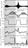 |
Fig. A.1 Example of application of the algorithm for the detection of jumps in the stream of K = G-1 values (Eq. 1) for LFI-27M during Planck’s first year. Panel A): the set of calibration constants K computed by Da Capo for LFI27M. The x-axis here is cropped to the first two sky surveys (one year of data). Panel B): the amplitude of the dipole signal, δTdip, as seen within each ring by the Planck spacecraft. The two horizontal lines mark the thresholds for regions where the signal is considered either strong or weak. Panel C): the size N of the window used to compute the moving average of K (there are roughly N = 30 values of K per day). In regions where the dipole signal is weak or strong, the window width is 1200 or 400 samples, respectively; outside such regions, we use a linear interpolation between these two values. Panel D): the result of applying a moving average with the variable window size (Panel C)) to the series of data shown in Panel A). This is not the smoothed series used for calibration; only the rms of the moving average is used (see next panel). Panel E): the figure of merit used to detect jumps is the product of the dipole amplitude and the rms of the moving average. The threshold used to detect jumps in this particular example (LFI-27M) is equal to the 99th percentile of such values (grey dashed line). In this case, two jumps have been found (days 257 and 450). |
In the 2015 Planck data release, we have improved our smoothing filter in order to consider sudden jumps in the calibration constant that are caused by a genuine change in the state of the radiometer; we call these real jumps. Such real jumps are not statistical effects and it is therefore incorrect to include them when smoothing the data. The actual smoothing algorithm used in the 2015 Planck-LFI data release works as follows:
-
1.
determine if there are sudden variations in the calibrationconstants that might have a non-statistical origin and make a list ofthem;
-
2.
split the stream of calibration constants into sub-streams, using the jumps found in the previous step;
-
3.
apply a low-pass filter to each sub-stream defined in the previous step as boundaries.
In the following paragraphs, we provide more details about the implementation of these steps.
Appendix A.2: Detecting jumps in the calibration constants
We discuss here how our data analysis code is able to determine the presence of sudden jumps in the calibration constant that are due to some real change in the state of the radiometer. This task is not trivial, since we must look for sudden variations in a stream of numbers (the K values) that is dominated by statistical noise; moreover, the rms of such data changes with time, since it is correlated with the amplitude of the dipole signal ΔTdip (see Fig. 4). Within a region of high rms, it is therefore possible to mistake a sudden change in the value of K due to statistical fluctuations with an intrinsic change in the radiometer’s calibration. We have therefore developed a figure of merit that allows us to disentangle these two families of jumps.
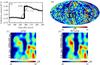 |
Fig. A.2 Comparison between the behaviour of the smoothing code in the nominal case and in the case where the jump near day 257 is considered to be a statistical fluctuation. Panel A): value of the calibration constant in the two cases. Fast variations have been removed from the data to make the plot clearer. If the jump is not considered to be real by the algorithm, the smoothing stage introduces an increasing slope in the values (thin grey line). Panel B): map of the difference between the maps from Surveys 1 and 2 (the jump happened during the first survey), in ecliptic coordinates. Residual systematic effects produce stripes that are either aligned with the direction of the scan (i.e., perpendicular to the ecliptic plane) or with the Galactic plane. The black square highlights a region in the map that has been observed during the jump near day 257. Panel C): zoom into the region highlighted in panel B) (the difference between maps from Surveys 1 and 2), when the jump near day 257 has been considered real (see Panel A), thick black line). Panel D): the same as the previous panel, but data have been calibrated assuming no real jump near day 257 (Panel A), thin grey line). Features are sharper in the latter case, and therefore we can conclude that the former calibration produces better results. |
To implement our figure of merit, we have defined a procedure to quantify the level of statistical fluctuations in the data. Such a procedure is similar to a smoothing filter and we describe it with the aid of Fig. A.1, which shows its application to some real data (the values of K for radiometer LFI-27M, calculated during the first two sky surveys). As already described in Sect. 3, the variation in the statistical noise in K (panel A) is related to the strength of the dipole signal, i.e., the amplitude of ΔTdip (panel B). Therefore, in order to properly weight the importance of variations in the value of K, we apply a moving average to the stream of K values, where the amplitude of the window (panel C) depends on the value of ΔTdip. The result of the moving average (Ksm) is shown in panel D of Fig. A.1. For each window, the code computes the rms, σK, of the N values. This quantity depends both on the statistical noise and on the presence of real jumps in the value of K. Therefore, we use the expression 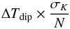 (A.1)as a figure of merit for determining the presence of real jumps. This quantity is proportional to the rms of the moving average but is weighted by the amplitude of the calibration signal: the stronger the latter, the more likely that a real jump is present in the N samples.
The threshold used with Eq. (A.1)is defined in terms of percentiles, specifically, we consider all the data that are greater than the nth percentile to mark the presence of a real jump. The value for n depends on the radiometer: for 30 GHz radiometers it is 99; for 44 GHz it is 99.9; and for 70 GHz it is 99.5. Such values have been determined by considering the quality of the null17 test (see Sect. A.4).
Appendix A.3: The smoothing algorithm
Once the positions of the jumps have been determined, the code applies a smoothing algorithm to each subset of values of the original K (produced by Da Capo) between two consecutive jumps. The algorithm applies a low-pass filter in the Fourier
domain that retains only 5% of the lowest frequencies. After this step, to further reduce the noise, we apply a moving average to the result, where each sample is weighted by the value of ΔTdip.
Appendix A.4: Validation of the algorithm
Since an incorrect identification of a real jump is likely to produce stripes in maps, we ran a number of null tests in order to optimize the free parameters of the smoothing algorithm (e.g., the threshold used to detect jumps and the widths of the moving average windows). We calibrated the data using a number of combinations of parameters and produced single-survey sky maps (i.e., maps obtained using six months of data). We then differenced them, under the hypothesis that a perfect calibration would produce a map where the value of each pixel is consistent with zero. Figure A.2 shows an example of this analysis and shows that the jump found by the code near day 257 is likely to be a real jump, because not considering it as such leads to a stronger stripe in survey-difference maps.
All Tables
Changes in the calibration level between this (2015) Planck-LFI data release and the previous (2013) one.
All Figures
|
Fig. 1 Schematics of an LFI radiometer taken from Cal13. The two linearized polarization components are separated by an orthomode transducer (OMT), and each of them enters a twin radiometer, only one of which is shown in the figure. A first amplification stage is provided in the cold (20 K) focal plane, where the signal is combined with a reference signal originating in a thermally stable 4.5-K thermal load. The radio frequency signal is then propagated through a set of composite waveguides to the warm (300 K) backend, where it is further amplified and filtered, and finally converted into a sequence of digitized numbers by an analogue-to-digital converter. The numbers are then compressed into packets and sent to Earth. |
| In the text | |
|
Fig. 2 Quantities used in determining the value of φsky (Eq. (8)) for radiometer LFI-27M (30 GHz) during a short time span (2 min). Panel A): the quantities Bmb ∗ TCMB and Bsl ∗ TCMB are compared. Fluctuations in the latter term are much smaller than those in the former. Panel B): the quantity Bsl ∗ TCMB shown in the previous panel is replotted here to highlight the features in its tiny fluctuations. That the pattern of fluctuations repeats twice depends on the scanning strategy of Planck, which observes the sky along the same circle many times with a spin rate of 1/60 Hz. Panel C): value of φsky calculated using Eq. (8). There are several values that diverge to infinity, which is due to the denominator in the equation going to zero. Panel D): distribution of the values of φsky plotted in panel C). The majority of the values fall around the number + 0.02%. |
| In the text | |
|
Fig. 3 Diagram of the pipeline used to produce the LFI frequency maps in the 2015 Planck data release. The grey ovals represent input/output data for the modules of the calibration pipeline, which are represented as white boxes. The product of the pipeline is a set of calibrated timelines that are passed as input to the mapmaker. |
| In the text | |
|
Fig. 4 Variation in time of a few quantities relevant for calibration for radiometers LFI-21M (70 GHz, left) and LFI-27M (30 GHz, right). Grey/white bands indicatecomplete sky surveys. All temperatures are thermodynamic. Panel A): calibration constant K estimated using the expected amplitude of the CMB dipole. The uncertainty associated with the estimate changes with time, according to the amplitude of the dipole as seen in each ring. Panel B): expected peak-to-peak difference in the dipole signal (solar + orbital). The shape of the curve depends on the scanning strategy of Planck, and it is strongly correlated with the uncertainty in the gain constant (see panel A)). The deepest minima happen during Surveys 2 and 4; because of the higher uncertainties in the calibration (and the consequent bias in the maps), these surveys have been neglected in some of the analyses in this Planck data release (see, e.g., Planck Collaboration XIII 2016). Panel C): the calibration constants K used to actually calibrate the data for this Planck data release are derived by applying a smoothing filter to the raw gains in panel A). Details regarding the smoothing filter are presented in Appendix A. |
| In the text | |
|
Fig. 5 Visual representation of the algorithms used to filter the calibration constants produced by DaCapo (top left plot; see Sect. 4). The example in the figure refers to radiometer LFI-27M (30 GHz) and only shows the first part of the data (roughly three surveys). |
| In the text | |
|
Fig. 6 Dipole amplitudes and directions for different radiometers. Top: errors in the estimation of the solar dipole direction are represented as ellipses. Bottom: estimates of the amplitude of the solar dipole signal; the errors here are dominated by gain uncertainties. Inset: the linear trend (recalling that the numbering of horns is approximately from left to right in the focal plane with respect to the scan direction), most likely caused by a slight symmetric sidelobe residual, is removed when we pair the 70 GHz horns. |
| In the text | |
|
Fig. 7 Top: estimate of the value of φD (Eq. (6)) for each LFI radiometer during the whole mission. The plot shows the median value of φD over all the samples and the 25th and 75th percentiles (upper and lower bar). These bars provide an idea of the range of variability of the quantity during the mission; they are not an error estimate of the quantity itself. Bottom: estimate of the value of φsky (Eq. (8)). The points and bars have the same meaning as in the plot above. Because of the low value for the 44 and 70 GHz channels, the inset shows a zoom of their median values. The large bars for the 30 GHz channels are motivated by the coupling between the stronger foregrounds and the relatively large power falling in the sidelobes. |
| In the text | |
|
Fig. 8 Top: comparison between the measured and estimated ratios of the aℓm harmonic coefficients for the nominal maps (produced using the full knowledge of the beam B over the 4π sphere) and the maps produced under the assumption of a pencil beam. The estimate has been computed using Eq. (11). Bottom: difference between the measured ratio and the estimate. The agreement is better than 0.03% for all 22 LFI radiometers. |
| In the text | |
|
Fig. 9 Top: impact on the average value of the aℓm spherical harmonic coefficients (computed using Eq. (42), with 100 ≤ ℓ ≤ 250) because of several improvements in the LFI calibration pipeline, from the first to the second data release. Bottom: measured change in the aℓm harmonic coefficients between the first and the second data releases. No beam window function has been applied. These values are compared with the estimates produced using Eq. (43), which assumes perfect independence among the effects. |
| In the text | |
|
Fig. 10 Discrepancy among the radiometers of the same frequency in the height of the power spectrum Cℓ near the first peak. For a discussion of how these values were computed, see the text. Inset: to better understand the linear trend in the 70 GHz radiometers, we have computed the weighted average between pairs of radiometers whose position in the focal plane is symmetric. The six points refer to the combinations 18M/23M, 18S/23S, 19M/22M, 19S/22S, 20M/21M, and 20S/21S, respectively. All six points are consistent with zero within 1σ; see also Fig. 6. |
| In the text | |
|
Fig. 11 Estimate of |
| In the text | |
|
Fig. 12 Difference in the application of the full 4π beam model versus the pencil beam approximation. Panel A): difference between survey 1 and survey 2 for a 30 GHz radiometer (LFI-27S) with the 4π model, smoothed to 15°. We do not show the same difference with pencil beam approximation, because it would appear indistinguishable from the 4π map. Panel B): double difference between the 4π1-2 survey difference map in panel A and the pencil difference map (not shown here). This map shows what changes when one drops the pencil approximation and uses the full shape of the beam in the calibration. Panel C): zoom on the blue spot visible at the top of the map in panel A). Panel D): same zoom for the pencil approximation map. The comparison between panels C) and D) shows that the 4π calibration produces better results. |
| In the text | |
|
Fig. 13 Visual timeline of Jupiters’s crossings with LFI beams. Here SS lables sky surveys. |
| In the text | |
|
Fig. 14 Time dependence of the angle between Jupiter’s direction and the spin axis of the Planck spacecraft. The darker horizontal bar indicates the angular region of the 11 LFI beam axes, and the lighter bar is enlarged by ± 5°. |
| In the text | |
|
Fig. 15 Distribution of the values of TB for Jupiter measured by the 22 LFI radiometers during each of the seven transits. The histogram has been produced using five bins per frequency. The lack of Gaussianity in the three distributions is evident. |
| In the text | |
|
Fig. 16 Distribution of the values of Tb for Jupiter as a function of the central frequency νcen of each radiometer. |
| In the text | |
|
Fig. 17 Top: brightness temperature of Jupiter (Tbr) compared with the data from Weiland et al. (2011), linearly rescaled in frequency to match LFI’s central frequencies νcen and corrected for difference between the LFI and WMAP dipoles. Bottom: deviation from unity of the ratio between LFI’s estimate for Tbr and WMAP’s. The agreement is excellent among the three frequencies. |
| In the text | |
|
Fig. A.1 Example of application of the algorithm for the detection of jumps in the stream of K = G-1 values (Eq. 1) for LFI-27M during Planck’s first year. Panel A): the set of calibration constants K computed by Da Capo for LFI27M. The x-axis here is cropped to the first two sky surveys (one year of data). Panel B): the amplitude of the dipole signal, δTdip, as seen within each ring by the Planck spacecraft. The two horizontal lines mark the thresholds for regions where the signal is considered either strong or weak. Panel C): the size N of the window used to compute the moving average of K (there are roughly N = 30 values of K per day). In regions where the dipole signal is weak or strong, the window width is 1200 or 400 samples, respectively; outside such regions, we use a linear interpolation between these two values. Panel D): the result of applying a moving average with the variable window size (Panel C)) to the series of data shown in Panel A). This is not the smoothed series used for calibration; only the rms of the moving average is used (see next panel). Panel E): the figure of merit used to detect jumps is the product of the dipole amplitude and the rms of the moving average. The threshold used to detect jumps in this particular example (LFI-27M) is equal to the 99th percentile of such values (grey dashed line). In this case, two jumps have been found (days 257 and 450). |
| In the text | |
|
Fig. A.2 Comparison between the behaviour of the smoothing code in the nominal case and in the case where the jump near day 257 is considered to be a statistical fluctuation. Panel A): value of the calibration constant in the two cases. Fast variations have been removed from the data to make the plot clearer. If the jump is not considered to be real by the algorithm, the smoothing stage introduces an increasing slope in the values (thin grey line). Panel B): map of the difference between the maps from Surveys 1 and 2 (the jump happened during the first survey), in ecliptic coordinates. Residual systematic effects produce stripes that are either aligned with the direction of the scan (i.e., perpendicular to the ecliptic plane) or with the Galactic plane. The black square highlights a region in the map that has been observed during the jump near day 257. Panel C): zoom into the region highlighted in panel B) (the difference between maps from Surveys 1 and 2), when the jump near day 257 has been considered real (see Panel A), thick black line). Panel D): the same as the previous panel, but data have been calibrated assuming no real jump near day 257 (Panel A), thin grey line). Features are sharper in the latter case, and therefore we can conclude that the former calibration produces better results. |
| In the text | |
Current usage metrics show cumulative count of Article Views (full-text article views including HTML views, PDF and ePub downloads, according to the available data) and Abstracts Views on Vision4Press platform.
Data correspond to usage on the plateform after 2015. The current usage metrics is available 48-96 hours after online publication and is updated daily on week days.
Initial download of the metrics may take a while.