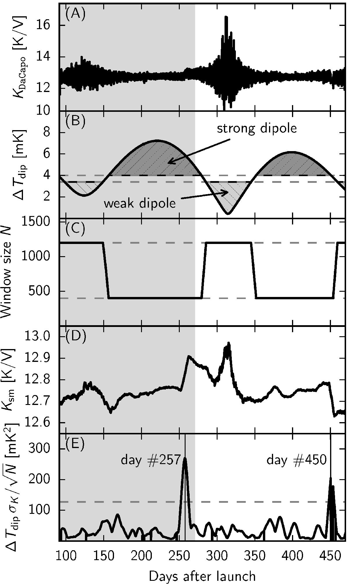
Example of application of the algorithm for the detection of jumps in the stream of K = G^-1 values (Eq. 1) for LFI-27M during Planck’s first year. Panel A): the set of calibration constants K computed by Da Capo for LFI27M. The x-axis here is cropped to the first two sky surveys (one year of data). Panel B): the amplitude of the dipole signal, δT_dip, as seen within each ring by the Planck spacecraft. The two horizontal lines mark the thresholds for regions where the signal is considered either strong or weak. Panel C): the size N of the window used to compute the moving average of K (there are roughly N = 30 values of K per day). In regions where the dipole signal is weak or strong, the window width is 1200 or 400 samples, respectively; outside such regions, we use a linear interpolation between these two values. Panel D): the result of applying a moving average with the variable window size (Panel C)) to the series of data shown in Panel A). This is not the smoothed series used for calibration; only the rms of the moving average is used (see next panel). Panel E): the figure of merit used to detect jumps is the product of the dipole amplitude and the rms of the moving average. The threshold used to detect jumps in this particular example (LFI-27M) is equal to the 99th percentile of such values (grey dashed line). In this case, two jumps have been found (days 257 and 450).