| Issue |
A&A
Volume 571, November 2014
Planck 2013 results
|
|
|---|---|---|
| Article Number | A28 | |
| Number of page(s) | 22 | |
| Section | Catalogs and data | |
| DOI | https://doi.org/10.1051/0004-6361/201321524 | |
| Published online | 29 October 2014 | |
Planck 2013 results. XXVIII. The Planck Catalogue of Compact Sources
1
APC, AstroParticule et Cosmologie, Université Paris Diderot, CNRS/IN2P3,
CEA/lrfu, Observatoire de Paris, Sorbonne Paris Cité, 10 rue Alice Domon et Léonie Duquet ;
75205
Paris Cedex 13 ;
France
2
Aalto University Metsähovi Radio Observatory and Dept of Radio
Science and Engineering, PO Box
13000, 00076
AALTO,
Finland
3
African Institute for Mathematical Sciences,
6-8 Melrose Road, 7945 Muizenberg,
Cape Town, South
Africa
4
Agenzia Spaziale Italiana Science Data Center,
via del Politecnico snc,
00133
Roma,
Italy
5
Agenzia Spaziale Italiana, Viale Liegi 26, 00198
Roma,
Italy
6
Astrophysics Group, Cavendish Laboratory, University of
Cambridge, J J Thomson
Avenue, Cambridge
CB3 0HE,
UK
7
Astrophysics & Cosmology Research Unit, School of
Mathematics, Statistics & Computer Science, University of
KwaZulu-Natal, Westville Campus,
Private Bag X54001, 4000
Durban, South
Africa
8
Atacama Large Millimeter/submillimeter Array, ALMA Santiago Central
Offices, Alonso de Cordova 3107,
Vitacura, Casilla
763 0355, Santiago, Chile
9
CITA, University of Toronto, 60 St. George St., Toronto, ON
M5S 3H8,
Canada
10
CNRS, IRAP, 9 Av.
colonel Roche, BP
44346, 31028
Toulouse Cedex 4,
France
11
California Institute of Technology, Pasadena, California, USA
12
Centre for Theoretical Cosmology, DAMTP, University of
Cambridge, Wilberforce
Road, Cambridge
CB3 0WA,
UK
13
Centro de Estudios de Física del Cosmos de Aragón (CEFCA), Plaza San
Juan, 1, planta 2, 44001
Teruel,
Spain
14
Computational Cosmology Center, Lawrence Berkeley National
Laboratory, Berkeley,
California,
USA
15
Consejo Superior de Investigaciones Científicas
(CSIC), 28006
Madrid,
Spain
16
DSM/Irfu/SPP, CEA-Saclay, 91191
Gif-sur-Yvette Cedex,
France
17
DTU Space, National Space Institute, Technical University of
Denmark, Elektrovej
327, 2800
Kgs. Lyngby,
Denmark
18
Département de Physique Théorique, Université de
Genève, 24 quai E.
Ansermet, 1211
Genève 4,
Switzerland
19
Departamento de Física Fundamental, Facultad de Ciencias,
Universidad de Salamanca, 37008
Salamanca,
Spain
20
Departamento de Física, Universidad de Oviedo,
Avda. Calvo Sotelo s/n,
33007
Oviedo,
Spain
21
Departamento de Matemáticas, Universidad de Oviedo,
Avda. Calvo Sotelo s/n,
33007
Oviedo,
Spain
22
Department of Astronomy and Astrophysics, University of
Toronto, 50 Saint George Street,
Toronto, Ontario,
Canada
23
Department of Astrophysics/IMAPP, Radboud University
Nijmegen, PO Box
9010, 6500 GL
Nijmegen, The
Netherlands
24
Department of Electrical Engineering and Computer Sciences,
University of California, Berkeley, California, USA
25
Department of Physics & Astronomy, University of British
Columbia, 6224 Agricultural Road,
Vancouver, British
Columbia, Canada
26
Department of Physics and Astronomy, Dana and David Dornsife College
of Letter, Arts and Sciences, University of Southern California,
Los Angeles, CA
90089,
USA
27
Department of Physics and Astronomy, University College
London, London
WC1E 6BT,
UK
28
Department of Physics, Florida State University,
Keen Physics Building, 77 Chieftan
Way, Tallahassee,
Florida,
USA
29
Department of Physics, Gustaf Hällströmin katu 2a, University of
Helsinki, 00014
Helsinki,
Finland
30
Department of Physics, Princeton University,
Princeton, New Jersey, USA
31
Department of Physics, University of California,
One Shields Avenue, Davis, California, USA
32
Department of Physics, University of California,
Santa Barbara, California, USA
33
Department of Physics, University of Illinois at
Urbana-Champaign, 1110 West Green
Street, Urbana,
Illinois,
USA
34
Dipartimento di Fisica e Astronomia G. Galilei, Università degli
Studi di Padova, via Marzolo
8, 35131
Padova,
Italy
35
Dipartimento di Fisica e Scienze della Terra, Università di
Ferrara, via Saragat
1, 44122
Ferrara,
Italy
36
Dipartimento di Fisica, Università La Sapienza,
P. le A. Moro 2, 00185
Roma,
Italy
37
Dipartimento di Fisica, Università degli Studi di
Milano, via Celoria,
16, 20133
Milano,
Italy
38
Dipartimento di Fisica, Università degli Studi di
Trieste, via A. Valerio
2, Trieste,
Italy
39
Dipartimento di Fisica, Università di Roma Tor
Vergata, via della Ricerca Scientifica,
1, Roma,
Italy
40
DiscoveryCenter, Niels Bohr Institute, Blegdamsvej 17, Copenhagen, Denmark
41
Dpto. Astrofísica, Universidad de La Laguna (ULL),
38206, La Laguna, Tenerife, Spain
42
European Southern Observatory, ESO Vitacura, Alonso de Cordova 3107, Vitacura, Casilla
19001
Santiago,
Chile
43
European Space Agency, ESAC, Planck Science Office, Camino bajo del
Castillo, s/n, Urbanización Villafranca del Castillo, Villanueva de la
Cañada, 28691
Madrid,
Spain
44
European Space Agency, ESTEC, Keplerlaan 1,
2201 AZ
Noordwijk, The
Netherlands
45
Finnish Centre for Astronomy with ESO (FINCA), University of
Turku, Väisäläntie 20,
21500, Piikkiö,
Finland
46
Haverford College Astronomy Department, 370 Lancaster Avenue, Haverford, Pennsylvania, USA
47
Helsinki Institute of Physics, Gustaf Hällströmin katu 2, University
of Helsinki, 00014
Helsinki,
Finland
48
INAF – Osservatorio Astrofisico di Catania, via S. Sofia
78, 95123
Catania,
Italy
49
INAF – Osservatorio Astronomico di Padova, Vicolo dell’Osservatorio
5, 35122
Padova,
Italy
50
INAF – Osservatorio Astronomico di Roma, via di Frascati
33, 00040
Monte Porzio Catone,
Italy
51
INAF – Osservatorio Astronomico di Trieste, via G.B. Tiepolo
11, 34131
Trieste,
Italy
52
INAF Istituto di Radioastronomia, via P. Gobetti 101,
40129
Bologna,
Italy
53
INAF/IASF Bologna, via Gobetti 101, 40129
Bologna,
Italy
54
INAF/IASF Milano, via E. Bassini 15, 20133
Milano,
Italy
55
INFN, Sezione di Bologna, via Irnerio 46,
40126
Bologna,
Italy
56
INFN, Sezione di Roma 1, Università di Roma Sapienza,
Piazzale Aldo Moro 2,
00185
Roma,
Italy
57
IPAG: Institut de Planétologie et d’Astrophysique de Grenoble,
Université Joseph Fourier, Grenoble 1/CNRS-INSU, UMR 5274, 38041
Grenoble,
France
58
ISDC Data Centre for Astrophysics, University of
Geneva, Ch. d’Ecogia
16, 1290
Versoix,
Switzerland
59
IUCAA, Post Bag 4, Ganeshkhind, Pune University
Campus, 411 007
Pune,
India
60
Imperial College London, Astrophysics group, Blackett
Laboratory, Prince Consort
Road, London,
SW7 2AZ,
UK
61
Infrared Processing and Analysis Center, California Institute of
Technology, Pasadena,
CA
91125,
USA
62
Institut Néel, CNRS, Université Joseph Fourier Grenoble
I, 25 rue des
Martyrs, 38042
Grenoble,
France
63
Institut Universitaire de France, 103 bd Saint-Michel, 75005
Paris,
France
64
Institut d’Astrophysique Spatiale, CNRS (UMR 8617) Université
Paris-Sud 11, Bât.
121, 91405
Orsay,
France
65
Institut d’Astrophysique de Paris, CNRS (UMR 7095),
98bis boulevard Arago, 75014,
Paris,
France
66
Institute for Space Sciences, 077125
Bucharest-Magurale,
Romania
67
Institute of Astronomy and Astrophysics, Academia
Sinica, 10617
Taipei,
Taiwan
68
Institute of Astronomy, University of Cambridge,
Madingley Road, Cambridge
CB3 0HA,
UK
69
Institute of Theoretical Astrophysics, University of
Oslo, 1029 Blindern,
0315
Oslo,
Norway
70
Instituto de Astrofísica de Canarias, C/Vía Láctea s/n, 38205 La Laguna, Tenerife, Spain
71
Instituto de Física de Cantabria (CSIC-Universidad de
Cantabria), Avda. de los Castros
s/n, 39005
Santander,
Spain
72
Jet Propulsion Laboratory, California Institute of
Technology, 4800 Oak Grove
Drive, Pasadena,
California,
USA
73
Jodrell Bank Centre for Astrophysics, Alan Turing Building, School
of Physics and Astronomy, The University of Manchester, Oxford Road, Manchester, M13
9PL, UK
74
Kavli Institute for Cosmology Cambridge,
Madingley Road, Cambridge, CB3 0HA, UK
75
LAL, Université Paris-Sud, CNRS/IN2P3, 91898
Orsay,
France
76
LERMA, CNRS, Observatoire de Paris, 61 avenue de
l’Observatoire, 75014
Paris,
France
77
Laboratoire AIM, IRFU/Service d’Astrophysique – CEA/DSM – CNRS –
Université Paris Diderot, Bât. 709, CEA-Saclay, 91191
Gif-sur-Yvette Cedex,
France
78
Laboratoire Traitement et Communication de l’Information, CNRS (UMR
5141) and Télécom ParisTech, 46 rue
Barrault, 75634
Paris Cedex 13,
France
79
Laboratoire de Physique Subatomique et de Cosmologie, Université
Joseph Fourier Grenoble I, CNRS/IN2P3, Institut National Polytechnique de
Grenoble, 53 rue des
Martyrs, 38026
Grenoble Cedex,
France
80
Laboratoire de Physique Théorique, Université Paris-Sud 11 &
CNRS, Bât. 210,
91405
Orsay,
France
81
Lawrence Berkeley National Laboratory, Berkeley, California, USA
82
Max-Planck-Institut für Astrophysik, Karl-Schwarzschild-Str. 1, 85741 Garching, Germany
83
McGill Physics, Ernest Rutherford Physics Building, McGill
University, 3600 rue University, Montréal, QC,
H3A 2T8,
Canada
84
MilliLab, VTT Technical Research Centre of Finland, Tietotie
3, 02044
Espoo,
Finland
85
National University of Ireland, Department of Experimental
Physics, Maynooth,
Co. Kildare,
Ireland
86
Niels Bohr Institute, Blegdamsvej 17, Copenhagen, Denmark
87
Observational Cosmology, Mail Stop 367-17, California Institute of
Technology, Pasadena,
CA
91125,
USA
88
Optical Science Laboratory, University College London,
Gower Street, London, UK
89
SB-ITP-LPPC, EPFL, 1015
Lausanne,
Switzerland
90
SISSA, Astrophysics Sector, via Bonomea 265,
34136
Trieste,
Italy
91
School of Physics and Astronomy, Cardiff University,
Queens Buildings, The Parade,
Cardiff, CF24 3AA, UK
92
Space Research Institute (IKI), Russian Academy of
Sciences, Profsoyuznaya Str,
84/32, 117997
Moscow,
Russia
93
Space Sciences Laboratory, University of California,
Berkeley, California, USA
94
Special Astrophysical Observatory, Russian Academy of
Sciences, Nizhnij Arkhyz,
Zelenchukskiy region, 369167
Karachai-Cherkessian Republic,
Russia
95
Stanford University, Dept of Physics, Varian Physics Bldg, 382 via Pueblo
Mall, Stanford,
California,
USA
96
Sub-Department of Astrophysics, University of Oxford,
Keble Road, Oxford
OX1 3RH,
UK
97
Theory Division, PH-TH, CERN, 1211, 23
Geneva,
Switzerland
98
UPMC Univ Paris 06, UMR7095, 98bis boulevard Arago, 75014
Paris,
France
99
Université de Toulouse, UPS-OMP, IRAP, 31028
Toulouse Cedex 4,
France
100
Universities Space Research Association, Stratospheric Observatory
for Infrared Astronomy, MS
232-11, Moffett
Field, CA
94035,
USA
101
University of Granada, Departamento de Física Teórica y del Cosmos,
Facultad de Ciencias, 18071
Granada,
Spain
102
Warsaw University Observatory, Aleje Ujazdowskie 4, 00-478
Warszawa,
Poland
Received:
21
March
2013
Accepted:
26
November
2013
The Planck Catalogue of Compact Sources (PCCS) is the catalogue of sources detected in the first 15 months of Planck operations, the “nominal” mission. It consists of nine single-frequency catalogues of compact sources, both Galactic and extragalactic, detected over the entire sky. The PCCS covers the frequency range 30–857 GHz with higher sensitivity (it is 90% complete at 180 mJy in the best channel) and better angular resolution (from 32.88′ to 4.33′) than previous all-sky surveys in this frequency band. By construction its reliability is >80% and more than 65% of the sources have been detected in at least two contiguous Planck channels. In this paper we present the construction and validation of the PCCS, its contents and its statistical characterization.
Key words: cosmology: observations / radio continuum: general / submillimeter: general
© ESO, 2014
1. Introduction
This paper, one of a set associated with the 2013 release of data from the Planck1 mission (Planck Collaboration I 2014), describes the first release of the Planck Catalogue of Compact Sources (PCCS).
The main goal of the Planck mission is to measure anisotropies in the cosmic microwave background (CMB), the relic radiation of the big bang; this radiation is “contaminated” by foreground emission arising from cosmic structures of all scales located between the CMB and us – galaxies, galaxy clusters, and gas and dust distributed on small as well as large scales within the Milky Way. In order to reveal the rich cosmological information concealed in the CMB such foreground emission must be characterized and separated (Planck Collaboration XII 2014). As a by-product, the study of foregrounds delivers an extensive catalogue of discrete compact sources as well as a series of maps of the Galactic diffuse emission; both of these are valuable resources for a variety of studies in the fields of Galactic and extragalactic astrophysics (e.g. Planck Collaboration XIX 2011; Planck Collaboration Int. XIV 2014; Planck Collaboration VII 2011; Planck Collaboration XXIII 2011; Planck Collaboration XXIX 2014).
In 1983 the IRAS survey (Beichman et al. 1988) revolutionized astronomy with the discovery of ultra-luminous infrared galaxies and debris disks, etc and is still relevant to active astrophysical research 30 years after its completion. Planck is at longer wavelengths but at comparable depths and promises to provide the community with an invaluable data set from the radio to sub-mm for many years to come.
The Planck Early Release Compact Source Catalogue (ERCSC; Planck Collaboration VII 2011) presented catalogues of discrete sources detected during Planck’s first 1.6 all-sky surveys. It has already been exploited for follow-up observations (e.g., AMI Consortium et al. 2012; Kurinsky et al. 2013) and for astrophysical investigations including the first direct determination of the bright end of the extragalactic source counts at frequencies ≥100 GHz (Planck Collaboration Int. VII 2013); the study of the spectral properties of radio sources (Planck Collaboration XIII 2011; Planck Collaboration XIV 2011; Bonavera et al. 2011) and of their long-term variability (Chen et al. 2013); as well as accurate estimates of the luminosity function of dusty galaxies in the very local Universe (i.e., distances ≤100 Mpc) at several millimetre and submillimetre wavelengths (Negrello et al. 2013) and of their dust mass and star-formation rate functions (Clemens et al. 2013). Moreover, a z = 3.26 strongly lensed submillimetre galaxy detected within the ≃135 deg2 of the phase 1 Herschel-ATLAS survey and possibly associated with a proto-cluster of dusty galaxies was found to be associated with an ERCSC source (Herranz et al. 2013; Fu et al. 2012), highlighting the potential of Planck surveys for detecting extremely high-redshift sources.
This paper presents a new Planck catalogue, the PCCS, which uses deeper observations (from the first 15 months of Planck operations) and better calibration and analysis procedures (Planck Collaboration II 2014; Planck Collaboration III 2014; Planck Collaboration V 2014; Planck Collaboration VI 2014; Planck Collaboration X 2014; Planck Collaboration VIII 2014) to improve on the results from the ERCSC. The PCCS comprises nine single-frequency source lists, one for each Planck frequency band. It contains high-reliability sources, both Galactic and extragalactic, detected over the entire sky. The PCCS differs in philosophy from the ERCSC in that it puts more emphasis on the completeness of the catalogue, without greatly reducing the reliability of the detected sources (>80% by construction). A comparison of the PCCS and ERCSC results is presented in Sect. 4.3.
This paper describes the construction and content of the PCCS; scientific results from the catalogue will appear in later papers. In Sect. 2 we describe the data, source detection pipelines, selection criteria, and photometry methods used in the production of the PCCS. In Sect. 3 we discuss the validation processes (both internal and external) performed to assess the quality of the catalogues. The main characteristics of the PCCS are summarized in Sect. 4, and a description of the content and use of the catalogue is presented in Sect. 5. Finally, in Sect. 6 we summarize our conclusions. Details of the different photometry estimators are described in Appendix A.
2. The Planck Catalogue of Compact Sources
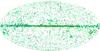 |
Fig. 1 Sky distribution of the PCCS sources at three different channels: 30 GHz (pink circles); 143 GHz (magenta circles); and 857 GHz (green circles). The dimension of the circles is related to the brightness of the sources and the beam size of each channel. The figure is a full-sky Aitoff projection with the Galactic equator horizontal; longitude increases to the left with the Galactic centre in the centre of the map. |
PCCS characteristics.
2.1. Data
The data obtained from the Planck nominal mission between 2009 August 12 and 2010 November 27 have been processed into full-sky maps by the Low Frequency Instrument (LFI; 30–70 GHz) and High Frequency Instrument (HFI; 100–857 GHz) Data Processing Centres (DPCs) (see Planck Collaboration II 2014; Planck Collaboration VI 2014). The data consist of two complete sky surveys and 60% of the third survey. This implies that the flux densities of sources obtained from the nominal mission maps are the average of at least two observations separated by roughly six months.
The nine Planck frequency channel maps were used as input to the source detection pipelines. The CMB dipole is removed during the map making stage. For the highest-frequency channels, 353, 545, and 857 GHz, a model of the zodiacal emission (Planck Collaboration XIV 2014) was the only foreground emission subtracted from the maps before detecting the sources. The relevant properties of the frequency maps are summarized in Table 1.
2.2. Source detection pipelines
Compact sources were detected in each frequency map by looking for peaks after convolving with a linear filter that preserves the amplitude of the source while reducing both large scale structure (e.g., diffuse Galactic emission) and small scale fluctuations (e.g., instrumental noise) in the vicinity of the sources.
Although the matched filter is optimal for uniform Gaussian noise, the real data present additional challenges. For example, the power spectrum is needed to construct the matched filter and this quantity is not known a priori and has to be determined directly from the data. We have explored the performance of different filters using realistic Planck simulations, among them our implementation of a matched filter and the first and second members of the Mexican Hat wavelet family, MHW and MHW2 (González-Nuevo et al. 2006; López-Caniego et al. 2006), and for these particular data we have chosen the last of these, MHW2, which performs better than the MHW and similarly to the matched filter.
The MHW2 has only one free parameter, the scale R, to be locally optimized, and is less sensitive to artefacts (e.g., missing pixels) or very bright structures in the image, like those found in the Galactic plane. These bright structures introduce instabilities in the determination of the power spectrum needed to construct the matched filter and reduce its performance. The MHW2 is robust and gives good performance at all Galactic latitudes. Besides, it has previously been used to detect compact sources in astronomical images, including realistic simulations of Planck (López-Caniego et al. 2006; González-Nuevo et al. 2006; Leach et al. 2008) and data from WMAP (López-Caniego et al. 2007; Massardi et al. 2009).
The MHW2 filter in Fourier space is given by 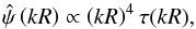 (1)where
k is the
wavenumber; τ
is the beam profile or point spread function, approximated by a Gaussian τ(x) = (1 /
2πσb2)
(1)where
k is the
wavenumber; τ
is the beam profile or point spread function, approximated by a Gaussian τ(x) = (1 /
2πσb2)![\hbox{$\exp[-\frac{1}{2}(\xx/\sigma_{\rm b})^2]$}](/articles/aa/full_html/2014/11/aa21524-13/aa21524-13-eq26.png) ; and σb is the
Gaussian beam dispersion.
; and σb is the
Gaussian beam dispersion.
Two independent implementations of the MHW2 algorithm have been used, one by the LFI DPC and another by the HFI DPC. The outputs of the two implementations have been compared and the results are compatible at the level of statistical uncertainty (see Sect. 2.5). An additional algorithm, the matrix filter (Herranz & Sanz 2008; Herranz et al. 2009), has been used to validate the catalogue; this is a multifrequency method that is also being used for the production of a multifrequency catalogue of non-thermal sources that will be published in a future paper.
The two MHW2 pipelines have a number of features in common. The full-sky HEALPix maps (Górski et al. 2005) are divided into small, square patch maps using a gnomonic projection. The patches should be large enough to get a fair sample of the noise in each, but small enough that the noise and foreground characteristics are close to uniform across each patch. The number of patches is chosen to allow sufficient overlap to remove detections in the borders of the patches where edge effects become important. In both pipelines the scale R of the filter is optimized by finding the maximum signal-to-noise ratio (S/N) of the sources in the filtered patch. The optimal scale is determined for each patch independently and, while it is always near to unity, it is usually smaller near the Galactic plane, e.g., 0.6 <R< 1.2 at 30 GHz, and bigger when the beam is smaller when compared to the pixel size, e.g., 1.1 <R< 1.5 at 70 GHz. Detections above a given S/N threshold are retained and the positions of the detected objects are translated from patch coordinates to spherical coordinates. The final stage is to remove multiple detections of the same object from different patches. No attempt has been made to remove detected sources from the maps.
LFI:
The compact source detection pipeline used in the LFI is part of the IFCAMEX software package2. It can be used to detect sources with no prior information on their position (blind mode), or at the position of known objects (non-blind mode). For this analysis we blindly search for objects over the full sky with S/N ≥ 2 to produce a preliminary catalogue of potential sources with positions, flux densities. and uncertainties. In the second step, IFCAMEX is run in non-blind mode, using as input the coordinates of the objects detected in the first step and keeping those with S/N ≥ 4. In this case the patch is centred on the position of the source. The goal of this second iteration is to minimize the already small border and projection effects and to refine the estimation of the position and S/N of each detection, keeping only those objects that still have a S/N above the threshold, and thus improving the reliability of the catalogue. In addition, and given the large size of the LFI beams, a fitting algorithm has been incorporated to find the centroids of the sources, achieving sub-pixel coordinate accuracy. Moreover, we have taken into account the effective non-Gaussian shape of the beams in the estimation of the flux density. This is done applying a correction factor to the IFCAMEX flux density estimation obtained by comparing the flux density of a simulated Gaussian test source of a given scale R with that of source convolved with the effective non-Gaussian beam of the detector at each of the LFI frequencies. This correction factor is small, typically <1%. Further details of this procedure can be found in Massardi et al. (2009).
HFI:
The novel features of the HFI implementation were designed to deal with the challenging environment for source detection in the high frequency channels. They aim to reduce the number of spurious detections with minimal impact on the number of real sources found. Each patch is filtered at the optimal scale, and also at four other scales bracketing the optimal scale. The dependence of the amplitude of the detection on the filter scale is compared with the predicted behaviour of a point source. The χ2 between the observed and predicted values is minimized to provide an alternative measurement of the amplitude. The values of the S/N, χ2, and the ratio of the two measurements of the amplitude determine whether a source is accepted or rejected. There is also an additional criterion for removing spurious detections that is based on the number of connected pixels, above a threshold, associated with a detection in the filtered patch at the optimal scale. The idea behind this is to reject artefacts that lie in narrow structures and may not be completely removed by the filtering. For the given scale of the wavelet, the number of expected connected pixels for a point source is evaluated and this is compared with the number of connections found for the detection. A combination of the S/N of the detection and the ratio of these numbers of connected pixels is used to determine whether rejection should occur. These additional criteria to reject artefacts help to improve the reliability of the catalogue without affecting its completeness and its other statistical properties.
2.3. Selection criteria
 |
Fig. 2 The Galactic and extragalactic zones used to define the S/N thresholds to meet the reliability target. The figure is a full-sky Mollweide projection. See text for further details. |
The source selection for the PCCS is made on the basis of the S/N. However, the background properties of the Planck maps vary substantially depending on frequency and part of the sky. Up to 217 GHz, the CMB is the dominant source of confusion at high Galactic latitudes. At high frequencies, confusion from Galactic foregrounds dominates the noise budget at low Galactic latitudes, and the cosmic infrared background at high Galactic latitudes. The S/N has therefore been adapted for each particular case.
The driving goal of the ERCSC was reliability greater than 90%. In order to increase completeness and explore possibly interesting new sources at fainter flux densities, however, a lower reliability goal of 80% was chosen for the PCCS. The S/N thresholds applied to each frequency channel have been determined, as far as possible, to meet this goal. The reliability of the catalogues has been assessed using the internal and external validation procedures described in Sect. 3.
At 30, 44, and 70 GHz, the reliability goal alone would permit S/N thresholds below 4. A secondary goal of minimizing the upward bias on fainter flux densities (Eddington bias; Eddington 1940) led to the imposition of an S/N threshold of 4.
At higher frequencies, where the confusion caused by the Galactic emission starts to become an issue, the sky has been divided into two zones, one Galactic (52% of the sky) and one extragalactic (48% of the sky), using the G45 mask defined in Planck Collaboration XV (2014). The zones are shown in Fig. 2. At 100, 143, and 217 GHz, the S/N threshold needed to achieve the target reliability is determined in the extragalactic zone, but applied uniformly across the sky. At 353, 545, and 857 GHz, the need to control confusion from Galactic cirrus emission led to the adoption of different S/N thresholds in the two zones. This strategy ensures interesting depth and good reliability in the extragalactic zone, but also high reliability in the Galactic zone. The extragalactic zone has a lower threshold than the Galactic zone. The S/N thresholds are given in Table 1.
2.4. Photometry
For each source in the PCCS we have obtained four different measures of the flux density. They are determined by the source detection algorithm; aperture photometry; point spread function (PSF) fitting; and Gaussian fitting. Only the first is obtained from the filtered maps, and the other measures are estimated from the full-sky maps at the positions of the sources. The source detection algorithm photometry, the aperture photometry and the PSF fitting use the Planck band-average effective beams, calculated with FEBeCoP (Fast Effective Beam Convolution in Pixel space; Mitra et al. 2011; Planck Collaboration IV 2014; Planck Collaboration VII 2014). Notice that only the PSF fitting uses a model of the PSF that depends on the position of the source and the scan pattern.
Detection pipeline photometry (DETFLUX).
As described in Sect. 2.2, the detection pipelines assume that sources are point-like. The amplitude of the detected source is converted to flux density using the area of the beam and the conversion from map units into intensity units. If a source is resolved its flux density will be underestimated. In this case it may be better to use the GAUFLUX estimation.
Aperture photometry (APERFLUX).
The flux density is estimated by integrating the data in a circular aperture centred at the position of the source. An annulus around the aperture is used to evaluate the level of the background. The annulus is also used to make a local estimate of the noise to calculate the uncertainty in the estimate of the flux density. The flux density is corrected for the fraction of the beam solid angle falling outside the aperture and for the fraction of the beam solid angle falling in the annulus. The aperture photometry was computed using an aperture with radius equal to the average full width at half maximum (FWHM) of the effective beam, and an annulus with an inner radius of 1 FWHM and an outer radius of 2 FWHM. The effective beams were used to compute the beam solid angle corrections. For details see Appendix A.1.
PSF fit photometry (PSFFLUX).
The flux density is obtained by fitting a model of the PSF at the position of the source to the data. The model has two free parameters, the amplitude of the source and a background offset. The PSF is obtained from the effective beam. For details see Appendix A.2.
Gaussian fit photometry (GAUFLUX).
The flux density is obtained by fitting an elliptical Gaussian model to the source. The Gaussian is centred at the position of the source and its amplitude, size, and axial ratio are allowed to vary, as is the background offset. The flux density is calculated from the amplitude and the area of the Gaussian. For details see Appendix A.3.
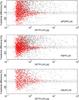 |
Fig. 3 Comparison of the APERFLUX, PSFFLUX and GAUFLUX flux density estimates with the DETFLUX ones for the 100 GHz catalogue, (S − SDETFLUX) /SDETFLUX. Grey points correspond to sources below | b | < 5° while red ones show the ones for | b | > 5°. Dashed lines indicates the ± 10% uncertainty level. |
Figure 3 shows a comparison between DETFLUX flux densities at 100 GHz and the other three estimates. DETFLUX has been chosen as the reference photometry because it is the photometry used in the selection process and the only one estimated directly from the filtered patches (filtering attenuates the background fluctuations by a factor ~2 and allows a much more robust estimation of the faintest flux densities). The dispersion increases at lower S/N and near the Galactic plane, where the different estimators behave differently in the presence of a strong background (indicated by grey points). At higher latitudes the agreement is much better for bright sources (the red points). This figure shows how the four different flux density estimators can provide complementary information on the same object, for example if the object is extended or near the Galactic plane (see Sect. 5.2).
2.5. Comparison between MHW2 pipelines
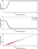 |
Fig. 4 Test of internal consistency between the two implementations of the MHW pipeline at 30 GHz for | b | > 30°. Top panel: cumulative percentage of sources detected by both methods. Middle panel: cumulative percentage of sources detected by only one of the methods. Bottom panel: comparison of the recovered flux densities (DETFLUX). |
In order to ensure the internal consistency of the whole catalogue, we have checked that both implementations of the MHW2 algorithm are equivalent. Both were run on the LFI nominal maps producing two sets of catalogues and the outputs from both implementations have been compared (see Fig. 4 for an example). We have studied the number of sources detected by both implementations (“matched”) and the number of sources detected by only one (“non-matched”). We have also compared the native (DETFLUX) photometry from both implementations. As shown in Fig. 4 for the 30 GHz channel, the only differences between the detections obtained by both implementations appear near the threshold where small changes in S/N values make the difference between a source being detected or not. These differences are always below 10% in the faintest bin. More important is the good agreement between photometric results from the two pipelines.
3. Validation of the PCCS
The PCCS contents and the four different flux-density estimates have been validated by simulations (internal validation) and comparison with other observations (external validation). The validation of the non-thermal radio sources can be done with a large number of existing catalogues, whereas the validation of thermal sources is mostly done with simulations. Detections identified with known sources have been marked in the catalogues.
3.1. Internal validation
The catalogues for the HFI channels have been validated primarily through an internal Monte Carlo quality assessment (QA) process in which artificial sources are injected in both real maps and simulated maps. For each channel, we calculate statistical quantities describing the quality of detection, photometry, and astrometry for each detection code. The detection is described by the completeness and reliability of the catalogue: completeness is a function of intrinsic flux density, the selection threshold applied to detection (S/N), and location, while reliability is a function only of the detection S/N. The quality of photometry and astrometry is assessed by direct comparison of detected position and flux density with the known parameters of the artificial sources. An input source is considered to be detected if a detection is made within one beam FWHM of the injected position.
The completeness is determined from the injection of unresolved point sources into the real maps. Bias due to the superimposition of sources is avoided by preventing injection within an exclusion radius of σb around both existing detections in the real map and previously injected sources. The flux from real and injected point sources contributes to the noise estimation for each detection patch, reducing the S/N of all detections and biasing the completeness. We prevent this effect by determining the noise properties on the maps before injecting sources, and have verified that remaining bias on detection and parameter estimates due to injected sources is negligible. The injected sources are convolved with the effective beam (Planck Collaboration II 2014; Planck Collaboration VI 2014).
We use two cumulative reliability estimates for the HFI catalogues. The first, which we will call simulation reliability, is determined from source injection into simulated maps and is defined as the fraction of detected sources that match the positions of injected sources. If the simulations are accurate, such that the spurious and real detection number counts mirror the real catalogue, the reliability is exact. To accept the simulations, we require that they pass the internal consistency tests outlined below. Simulation reliability is used for the 100, 143, and 217 GHz channels.
The simulations used to calculate simulation reliability consist of realizations of CMB, instrumental noise, and the diffuse Galactic emission component of the FFP6 simulations (a set of realistic simulations based on the Planck Sky Model; Planck Collaboration XII 2014; Planck Collaboration Int. VII 2013; Delabrouille et al. 2013). We require that the simulated catalogues pass two internal consistency tests: that they have the same injected source completeness as the real catalogues calculated as outlined above; and that they have total detected number counts, as a function of S/N, that are consistent with those in the real data. The intrinsic number counts are assumed to be power law functions of flux density and are fitted to the detection counts at higher flux densities, where the catalogues are reliable and complete, and extrapolated to lower flux densities. Sources are injected with random positions.
The second reliability estimator is applied to the 353, 545, and 857 GHz channels, where the simulations fail our internal consistency tests (due to deficiencies in the simulations of diffuse dust emission). In the absence of accurate simulations capable of producing realistic realisations of spurious detections, we use an approximate reliability criterion that we will call injection reliability. Injection reliability makes use of source injection into the real maps to determine number counts of matched sources. If the fiducial input source model is accurate, the matched counts are a good estimate of the real detection counts in the catalogue. To form a reliability estimate, we take the ratio per S/N bin of the matched number counts over the number counts of the real catalogue (the latter of which is the sum of real and spurious number counts).
The input flux density model is assumed to be a power law and is fitted in the same way as for the simulation reliability. The extrapolation of the input source model to lower flux densities is the main source of uncertainty in the injection reliability estimate. However, it is also subject to bias due to the Poisson fluctuations of number counts in the real catalogue. The total numbers are large enough at low S/N in the higher frequency channels that the measurement of the increment of spurious sources is robust to these fluctuations. At higher S/N, however, we take as reliable any bin where the difference between expected real and measured total number counts is smaller than twice the Poisson noise of the total number counts. To minimise bias from fluctuations, we also assume the catalogues are completely reliable at S/N> 10. We have verified that the two reliability estimates are consistent with one another at 217 GHz, the only frequency where they can both be applied.
3.1.1. Completeness
We have estimated the completeness of each of the HFI catalogues in the 48% extragalactic zone shown in Fig. 2. We have also estimated completeness in the larger zones outside two Galactic dust masks shown in Fig. 5: the less restrictive 85% zone for 100 GHz and 143 GHz, and the 65% zone for 217 GHz. These zones match those assumed for the reliability estimate at those channels. The completeness estimates are shown in Fig. 6, along with full-sky maps of the sensitivity, defined as the flux density at 50% differential completeness.
 |
Fig. 5 Galactic dust masks used to estimate completeness and reliability for some of the HFI channels. The unmasked zones correspond to sky fractions of 65% and 85%. The figure is a full-sky Mollweide projection. See text for further details. |
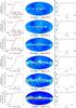 |
Fig. 6 Results of the internal validation for HFI channels. The quantities plotted are (left) completeness per bin, (middle) a map of sensitivity (the 50% completeness threshold in flux density), and (right) cumulative reliability as a function of S/N. The black curves in completeness are for the extragalactic zone described in Sect. 2.3. The red curves in completeness are for smaller masks used for the reliability estimation (if the extragalactic zone was not used). See text for discussion of the limitations of the injection reliability estimate used for 353 GHz and above. |
3.1.2. Reliability
The cumulative reliability, or fraction of detections above a given S/N that match a real source, is determined using the simulation reliability estimate for channels up to and including 217 GHz, and the injection reliability estimate at higher frequencies. These are shown in the right column of Fig. 6. For 100 GHz and 143 GHz, the reliability is calculated using the 85% Galactic dust mask, for 217 GHz using the 65% Galactic dust mask, and for the other channels using the 48% extragalactic zone. Injection reliability cannot accurately resolve the small departures from reliability at S/N> 5.8, due to Poisson noise. Some bins above this limit show departures from full reliability at greater than 2σ at 545 GHz and 857 GHz and these are responsible for the exaggerated stepping of the reliability. These fluctuations are likely purely statistical and are a limitation of the precision of injection reliability at higher S/N.
3.1.3. Photometry and astrometry
For the HFI channels we characterize the accuracy of source photometry by comparing the native flux density estimates (DETFLUX) of matched sources to the known flux densities of sources injected into the real maps. Examples of the distributions of photometric errors, for 143 GHz and 857 GHz, are shown in Fig. 7, which presents histograms of the quantity ΔS/σS, where ΔS is the difference between the estimated and the injected flux densities, and σS is the flux density uncertainty. The photometric accuracy is a function of S/N, with faint detections affected by upward bias due to noise fluctuations. At lower HFI frequencies, the DETFLUX estimates are unbiased for bright sources. At higher HFI frequencies, the DETFLUX estimates are biased low. Table 2 shows the DETFLUX bias per channel as well as the standard deviation of ΔS/σS (which would be unity for Gaussian noise).
We characterize the accuracy of the astrometry by calculating the radial position offset between the positions of detected sources and the known positions of the sources injected into the real maps. The distribution of the radial offsets is shown in Fig. 7 for 143 GHz and 857 GHz.
Native photometry (DETFLUX) bias (mean multiplicative), photometric recovery uncertainty, and median radial position uncertainty from the internal validation, all calculated in the extragalactic zone.
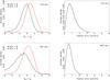 |
Fig. 7 Example distributions of photometric recovery (left) and positional error (right) for 143 GHz (top row) and 857 GHz (bottom row). |
3.2. External validation
3.2.1. Low frequencies: 30, 44, and 70 GHz
At the three lowest Planck frequencies, it is possible to validate the PCCS source identifications, completeness, reliability, positional accuracy, and in some case even flux density accuracy using external data sets, particularly large-area radio surveys. This external validation was undertaken using the following catalogues and surveys: (1) the full-sky NEWPS catalogue, based on WMAP maps (López-Caniego et al. 2007; Massardi et al. 2009); (2) in the southern hemisphere, the Australia Telescope 20 GHz survey (AT20G; Murphy et al. 2010); (3) in the northern hemisphere, where no large-area survey at similar frequencies to AT20G is available, the 8.4 GHz Combined Radio All-sky Targeted Eight GHz Survey (CRATES; Healey et al. 2007). These catalogues have comparable frequency coverage and source density to the PCCS. We also compared the PCCS with the Planck ERCSC: this provides a useful check on the PCCS pipelines, although the ERCSC is based on a subset of the data used for the PCCS and is not an independent catalogue. As discussed in Planck Collaboration VII (2011), more than 95% of the ERCSC sources had a clear counterpart in external catalogues.
For this comparison, a PCCS source is considered reliably identified if it falls within a circle of radius 0.65 times the Planck effective beam FWHM (see Table 1) that is centred on a source at the corresponding frequency found in one of the above catalogues. Of the four reference catalogues, only the ERCSC covers the Galactic plane and therefore for | b | < 2deg (the AT20G Galactic cut) the external validation relies on the previous identification effort performed for the ERCSC (Planck Collaboration XIV 2011).
Owing to its better sensitivity, the PCCS detects almost all the sources previously
found by WMAP (Bennett et al. 2013). Therefore,
for studying completeness, deeper samples like the AT20G or CRATES are needed. The
problem is that those samples are at lower frequencies (20 and 8.4 GHz, respectively)
than the LFI, so spectral effects or variability could in some cases put the sources
below the PCCS detection limit. The completeness values estimated by comparison with
these catalogues should thus be considered as lower limits. For this reason we used an
alternative completeness estimate that can be derived from knowledge of the noise in the
maps. If the native flux density estimates are subject to Gaussian errors with amplitude
given by the noise of the filtered patches, the completeness per patch should be
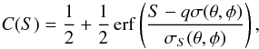 (2)where
 is the variance of the
filtered patch located at (θ,φ), q is the S/N threshold and
is the variance of the
filtered patch located at (θ,φ), q is the S/N threshold and
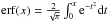 is the standard error
function. The true completeness will depart from this limit when the simplifying
assumptions of Gaussian noise and uniform Gaussian beams are broken. The cumulative
completeness is derived by making use of a model of the source counts N(S)
(de Zotti et al. 2005).
is the standard error
function. The true completeness will depart from this limit when the simplifying
assumptions of Gaussian noise and uniform Gaussian beams are broken. The cumulative
completeness is derived by making use of a model of the source counts N(S)
(de Zotti et al. 2005).
Figure 8 shows the estimated completeness and a summary of the external validation results at the LFI channels (30, 44, and 70 GHz), after combining the information from the four reference radio catalogues. The completeness at 90% level is also given in Table 1.
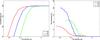 |
Fig. 8 External validation summary (completeness and number of non-matched sources) of the 30, 44, and 70 GHz channels. |
The unmatched sources are those detected by Planck and appearing in the PCCS, but not present in any of the reference catalogues. Many of them, however, are internally confirmed, either by a multifrequency detection method for the LFI frequencies or in adjacent HFI channels. Sources in this category are robust detections, and therefore are probably sources previously undetected at frequencies between 10 and 20 GHz or by IRAS at higher frequencies. The few remaining ones are likely to be peaks or structures in the distribution of Galactic emission, that may include supernova remnants, reflection nebulae, or planetary nebulae (AMI Consortium et al. 2012). They could also be faint thermal sources, or strongly variable ones. They may therefore constitute an interesting sample for follow-up observations. The status of the cross-matching is indicated in the EXT_VAL column in the PCCS (see Sect. 5.1).
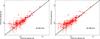 |
Fig. 9 Comparison between the PACO sample (Massardi et al. 2011; Bonavera et al. 2011; Bonaldi et al. 2013) and the extrapolated, colour-corrected PCCS flux densities (DETFLUX) at 32 (left) and 40 GHz (right). The multiple PACO observations of each source have been averaged to a single flux density and therefore the uncertainties reflect the variability of the sources instead of the actual flux density accuracy of the measurements (a few mJy). |
An absolute validation of the extracted photometry can be obtained by comparing the PCCS measurements with external data sets. For instance, the Planck Australia Telescope Compact Array (ATCA) Co-eval Observations (PACO; Massardi et al. 2011; Bonavera et al. 2011; Bonaldi et al. 2013) have provided flux density measurements of well-defined samples of AT20G sources at frequencies below and overlapping with Planck frequency bands, obtained almost simultaneously with Planck observations. A total of 482 sources have been observed in the frequency range between 4.5 and 40 GHz in the period between 2009 July and 2010 August. The multiple PACO observations have been averaged to a single flux density and therefore the uncertainties reflect the variability of the sources instead of the actual flux density accuracy of the measurements (typically, a few millijanskys). The comparison was performed at the PACO frequencies by extrapolating the PCCS flux densities using the spectral indices estimated between 30 and 44 GHz and taking into account the corresponding colour correction (Planck Collaboration II 2014; Planck Collaboration VI 2014). At both 30 and 44 GHz the two flux density scales appear to be in good overall agreement (− 4% ± 8% and 5% ± 10%, respectively) with any difference attributable partly to the background effect in the Planck measurements and partly to variability in the radio sources, since the PCCS and PACO measurements were not exactly simultaneous (see Fig. 9). In particular, the PCCS flux densities of the faintest sources are, on average, overestimated due to faint sources that exceed the detection threshold because they lie on top of positive intensity fluctuations. This effect, known as Eddington bias, can be statistically corrected (López-Caniego et al. 2007, Appendix B2; Crawford et al. 2010). Note however that it mostly affects sources below the 90% completeness limit.
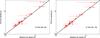 |
Fig. 10 Comparison between the Metsähovi and the colour-corrected PCCS flux densities (DETFLUX) interpolated to 37 GHz using 30 and 44 GHz Planck data (left) and 30 and 70 GHz data (right). The multiple observations of each source have been averaged to a single flux density and therefore the uncertainties reflect the variability of the sources instead of the actual flux density accuracy of the measurements (a few mJy). |
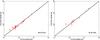 |
Fig. 11 Planck flux densities for bright sources observed within a month of VLA observations at that frequency. Planck values (APERFLUX) were colour-corrected and interpolated to ~28 GHz (left) and ~43 GHz (right). |
The Metsähovi observatory is continuously monitoring bright radio sources in the northern sky (Planck Collaboration XV 2011) at 37 GHz. From their sample, sources brighter than 2 Jy were selected and their flux densities averaged over the period of Planck observations used for the PCCS. As in the PACO case, the uncertainties in the plot reflect the variability of the sources during the Planck nominal mission period. The Planck measurements were colour-corrected and extrapolated to the Metsähovi frequency before the comparison (see Fig. 10). The Planck and Metsähovi flux densities agree at the 0.2% level with an uncertainty of ±4%.
On 2012 January 19–20, the Karl G. Jansky Very Large Array (VLA) was employed by Rick Perley of the NRAO staff to make observations of a number of bright, extragalactic radio sources also detected by Planck within a month of that date. The aim of these coordinated observations was to minimize scatter caused by the variability of bright radio sources, most of them blazars. The VLA observations were made at a number of frequencies, spanning the two lowest LFI frequencies. Planck data (APERFLUX), colour-corrected and interpolated to the VLA frequencies of 28.45 and 43.34 GHz, were compared with nearly simultaneous Planck observations (see Fig. 11 for the 43 GHz case). To lessen the effect of Eddington-like bias in the Planck data, the fit was forced to pass through (0,0). The slopes of the fitted lines show that the VLA and Planck flux densities agree to about 2 ± 1.6% at 28 GHz, with Planck slightly low. At 43 GHz the agreement is not as good, with Planck PCCS flux densities running ~6% high on average. This value, however, is driven by one source, 3C 84, known to be variable. If it is excluded, Planck and VLA flux densities at 44 GHz agree to ~0.5 ± 2.5%. The VLA flux density scale used in this comparison is the new one proposed by Perley & Butler (2013), based on observations of Mars.
3.2.2. Intermediate frequencies: 143 and 217 GHz
A similar comparison was made between Planck flux density measurements of around 40 sources catalogued by the Atacama Cosmology Telescope team (M. Gralla et al., in prep.). Planck 143 and 217 GHz measurements were colour-corrected and interpolated to match the band centres of the ACT 148 and 218 GHz channels. Since the ACT measurements were made over a wider span of time than the Planck ones, source variability introduces a scatter (see Fig. 12). Nevertheless, on average, Planck and ACT observations agree to 2.0 ± 2.5% at 148 GHz, and ~5.0 ± 3.5% at 218 GHz. If we exclude 2–4 variable sources, the agreement at 218 GHz improves to ~0.5 ± 3.5%.
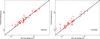 |
Fig. 12 Comparison between ACT and Planck measurements (DETFLUX; colour-corrected). Left panel: Planck measurements were extrapolated to 148 GHz. Planck flux densities are on average 1% fainter (or ACT’s brighter). The uncertainty in the slope is 0.025 = 2.5%. Right panel: Planck measurements were extrapolated to 218 GHz.The slope is 1.033: Planck flux densities are high (or ACT’s low) by 3.3 ± 3.4% on average. |
3.2.3. High frequencies: 353, 545, and 857 GHz
Figure 13 shows a comparison between Planck flux densities at 353 GHz and those from two SCUBA catalogues (Dale et al. 2005; Dunne et al. 2000 [SLUGS]) at 850 μm. A colour correction of 0.898 has been applied to the Planck flux densities (Planck Collaboration VI 2014). The flux densities are in broad agreement between the two catalogues. The uncertainties in SCUBA measurements for extended sources make it difficult to draw strong conclusions about the suitability of the four PCCS flux density estimates.
 |
Fig. 13 Comparison between SCUBA and Planck flux densities at 353 GHz. All four PCCS flux densities estimates are shown, from left to right, APERFLUX, PSFFLUX, GAUFLUX, and DETFLUX. A colour correction of 0.898 has been applied to the Planck flux densities. The vertical dashed line shows the 90% completeness level of the PCCS. The diagonals show the line of equality between the flux densities. |
The Herschel/SPIRE instrument (Griffin et al. 2010) is performing many science programs, among which the wide surveys (extragalactic and Galactic) can be used to cross-check the flux densities of SPIRE and HFI at the common channels: 857 GHz with 350 μm, and 545 GHz with 500 μm. The H-ATLAS survey (Eales et al. 2010) is of particular interest since many common bright sources (typically with flux densities above a few hundred millijanskys) can be compared.
Figure 14 shows the comparison between Planck flux densities at 545 and 857 GHz and four Herschel catalogues, HRS (Boselli et al. 2010), KINGFISH (Kennicutt et al. 2011), HeViCS (Davies et al. 2013), and H-ATLAS (Eales et al. 2010). Inter-calibration offsets between the two instruments were corrected prior to comparison (Planck Collaboration V 2014; Planck Collaboration VIII 2014). To compare with 545 GHz flux densities, the Herschel 500 μm data have been extrapolated to 550 μm (545 GHz) assuming a spectral index of 2.7, which is the mean value found for the matched objects. At 350 μm (857 GHz) no correction has been applied since the Herschel and Planck filters are nearly the same.
At low flux densities, the smallest dispersion is achieved by the DETFLUX photometry because the filtering process removes structure not associated with compact sources. At high flux densities, the brightest objects in the KINGFISH survey are extended galaxies that are resolved by Planck so their flux densities are underestimated by DETFLUX, APERFLUX and PSFFLUX. GAUFLUX accounts for the size of the source and is therefore able to estimate the flux density correctly. For extended sources like these, we recommend the use of GAUFLUX (see also Sect. 5.2).
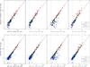 |
Fig. 14 Comparison between Herschel and Planck flux densities at 545 GHz (top) and 857 GHz (bottom). All four PCCS flux densities estimates are shown, from left to right, APERFLUX, PSFFLUX, GAUFLUX, and DETFLUX. The Herschel 500 μm data have been extrapolated to 550 μm (545 GHz) assuming a spectral index of 2.7. The vertical dashed line shows the 90% completeness level of the PCCS. The diagonals show the line of equality between the flux densities. |
All these results show that the flux density measurements in the PCCS are in reasonable agreement with those obtained at ground-based observatories or with higher resolution instruments like SCUBA and those of Herschel. That agreement, in turn, means that the solid angles of Planck beams are understood to comparable accuracy.
3.3. Comparison between internal and external validation
To check the consistency of the two validation processes, we extend the HFI internal validation to 70 GHz and compare with the results of the external validation. Simulations were constructed at 70 GHz as outlined in Sect. 3.1 and the injected sources were extracted using the HFI–MHW extraction algorithm. The simulations passed the internal consistency tests discussed in Sect. 3.1, allowing us to determine the reliability using simulation reliability estimate, as was the case for 100–217 GHz.
Figure 15 shows the completeness and reliability for the HFI–MHW and LFI–MHW catalogues as estimated using their respective validations at 70 GHz. We compare the external validation of the LFI–MHW catalogue with the internal validation of the HFI–MHW catalogue. Both the reliability and the completeness determined from each of the validations are in good agreement.
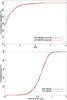 |
Fig. 15 Cumulative reliability (top panel) and differential completeness (bottom panel) of the HFI–MHW and LFI–MHW catalogues at 70 GHz as determined by their respective internal and external validation procedures. |
3.4. Impact of Galactic cirrus at high frequency
The intensity fluctuations in the Planck high-frequency maps are dominated by faint star-forming galaxies and Galactic cirrus (Condon 1974; Hacking et al. 1987; Franceschini et al. 1989; Helou & Beichman 1990; Toffolatti et al. 1998; Dole et al. 2003; Negrello et al. 2004; Dole et al. 2006). The filamentary structure of Galactic cirrus at small angular scales (from a few tens of arcseconds up to a few tens of arcminutes or a degree) is often visible as knots in Planck maps. These sources, which appear compact in the Planck maps, appear as filamentary structures when viewed by high-resolution instruments such as Herschel/SPIRE. An example is the Polaris field (see Fig. 16), where Herschel does not detect sources above the extragalactic density counts, but Planck detects a sharply increasing number of sources with lower interstellar brightness that are coincident with filaments.
Using the few Herschel fields available, we are able to establish a statistical evaluation of how the spurious source density behaves. We consider real sources to be compact structures that are not part of the interstellar quasi-stationary turbulent cascade. The other apparent sources are artefacts of the detection algorithms on the general interstellar structure and depend strongly on the angular resolution used. They are not useful as sources in a catalogue.
To control the spurious detections induced by the cirrus filaments, we apply higher S/N thresholds in the Galactic zone for 353, 545, and 857 GHz (see Table 1). These thresholds remove the bulk of the spurious sources identified in the Herschel SPIRE fields in this zone, while preserving the majority of the extragalactic compact objects.
For the extragalactic zone, we note that there is a local threshold in brightness that we estimate to be approximately 3–5 MJysr-1 at 857 GHz, above which the probability of cirrus-induced spurious detections increases. This is not used to threshold the catalogue, but could be used as a further control of spurious detections.
In some areas the situation is more complicated. Herschel does detect “real” Galactic (protostellar) sources in filaments in brighter regions (like the Aquila rift, André et al. 2010). These sources often are not fully unresolved but are embedded in an envelope and the filamentary structure. These sources usually lie in sky regions of much higher brightnesses, and are located within the Galactic zone.
We suggest a local definition of the presence of “real” Galactic sources: the power spectra of the maps at 857 GHz retain their power law behaviour all the way from large scales measured by Planck to the smallest scales measured by Herschel (with a very good overlap), with the flat part of the power spectrum after noise removal being at the level set by extragalactic sources. The power spectra of the fields considered in this analysis are shown in Fig. 17.
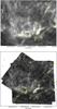 |
Fig. 16 The Polaris field observed by Planck (top) and Herschel (bottom) at 857 GHz (350 μm). Structures that appear to be compact sources to Planck, shown with yellow circles, are revealed to be cirrus knots when observed at higher resolution. They are located in regions with bright backgrounds, which provides a proxy for identifying them. The declination grid has spacing of 30 arc-min. |
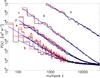 |
Fig. 17 Power spectra of six fields observed by both Planck (red) and Herschel (black). Fits to the spectra are shown in blue. There is a good agreement between Planck and Herschel in the common multipole range (typically ℓ< 3000). Fields are, from top to bottom: (a) Aquila; (b) Polaris; (c) Spider; (d) Draco; (e) Gama; (f) FLS; and (g) XMM-LSS. No real Galactic sources are expected in fields (b)–(g), only extragalactic sources (correlated and Poisson components) and cirrus at larger angular scales. Real Galactic sources are detected, however, in (a) (André et al. 2010): the power spectrum is orders of magnitude above the other fields, demonstrating the need to separate the Galactic from extragalactic zones, and the use of the background brightness as a proxy to estimate the cirrus contamination. |
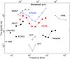 |
Fig. 18 The PCCS completeness level outside the Galactic plane (see Table 1) is shown relative to other wide area surveys. The ERCSC completeness levels have been obtained from Planck Collaboration XIII (2011) up to 70 GHz and Planck Collaboration Int. VII (2013) for the other channels, while the WMAP ones are from González-Nuevo et al. (2008) up to 41 GHz and Lanz et al. (2013) for 61 and 94 GHz. The sensitivity levels for Herschel SPIRE and PACS instruments are from Clements et al. (2010) and Rigby et al. (2011), respectively. The other wide area surveys shown as a comparison are: GB6 (Gregory et al. 1996), CRATES (Healey et al. 2007), AT20G (Murphy et al. 2010), PACO (Bonavera et al. 2011), SPT (Mocanu et al. 2013), ACT (Marsden et al. 2014) and IRAS (Beichman et al. 1988). |
4. Characteristics of the PCCS
4.1. Sensitivity and positional uncertainties
Table 1 shows the effective beam FWHM, the minimum flux density (after excluding the faintest 10% of sources) and the 90% completeness level of all nine lists in the PCCS. As an illustration, Fig. 18 shows the completeness level of PCCS at high Galactic latitude (| b | > 30°) relative to the previous ERCSC and other wide area surveys at comparable frequencies. It is clear from this comparison that the sensitivity of the PCCS is a significant improvement on that of the ERCSC (see Sect. 4.3) and that both catalogues are more complete than the WMAP ones. Note that the PCCS detection limit increases inside the Galactic plane.
Figure 6 shows how the sensitivity of the catalogues varies across the sky due to the scanning strategy (the minimum noise is at the ecliptic poles where the sky is observed many times) and due to the effect of Galactic emission (near the Galactic plane and in particular Galactic regions).
The positional accuracy of the ERCSC was confirmed to be better than FWHM/5 (Planck Collaboration VII 2011; Bonavera et al. 2011). In the case of the PCCS we have found similar results or better, as expected, since we have made corrections for two types of pointing errors that affected the ERCSC (Planck Collaboration VII 2011). The first was due to time-dependent, thermally-driven misalignment between the star tracker and the telescope (Planck Collaboration I 2014). The second was due to uncorrected stellar aberration across the focal plane. The misalignment resulting from stellar aberration is of the same magnitude as the positional uncertainties, and hence was not apparent in the ERCSC.
As explained in Sect. 3.2, by comparing the positions derived with the detection method used to build the PCCS with the PACO sample (Massardi et al. 2011; Bonavera et al. 2011; Bonaldi et al. 2013), we have estimated the distribution of the pointing uncertainties up to 353 GHz. In the case of 545 and 857 GHz we derived the same quantities from the comparison with Herschel sources. The median values of these distributions are reported in Table 1. The estimated positional uncertainties are below FWHM/5. These results are in good agreement with the values derived from the internal validation (see Table 2).
Summary of sources matched between neighbouring channels.
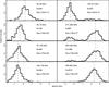 |
Fig. 19 Spectral indices of PCCS sources matched between contiguous channels with | b | > 30°. Each panel also shows the number of sources and the fraction with α> 1. The median values are indicated by vertical dashed lines. |
4.2. Statistical properties of the PCCS
Table 3 shows the numbers of sources internally matched within PCCS by finding them in neighbouring channels. It shows the number Nboth of sources matched both above and below in frequency (e.g., sources at 100 GHz found in both the 70 and 143 GHz catalogues), the number Neither matched either above or below in frequency (a less stringent criterion), and the fraction of sources so matched. A source is considered to be matched if the positions are closer than the larger FWHM of the two channels. A catalogue was extracted from the IRIS 100 μm map (Miville-Deschênes & Lagache 2005) using the MHW2 pipeline, and that is used as the neighbouring channel above 857 GHz. The IRIS mask, which removes around 2.1% of the sky, was applied to the 857 GHz catalogue before doing this comparison, and this reduces the number of sources to 24 119, a decrease of about 1%. The number of matches obtained for the 857 GHz channel only includes sources outside the IRIS mask. For the 30 GHz channel, the matches were evaluated using only the channel above, 44 GHz. The low percentage of internal matches of the 30 GHz channel results from two factors: the generally negative spectral index of the sources at these frequencies and the relatively low sensitivity of the 44 GHz receivers. In fact, when the sensitivity of one of the neighbouring channels is worse, the percentage of matched sources is lower, as is the case between 70 and 100 GHz and between 217 and 353 GHz.
Figure 19 shows histograms of the spectral indices obtained from the matches between contiguous channels. As expected, the high frequency channels (545 and 857 GHz) are dominated (>90%) by dusty galaxies and the low frequency ones are dominated (>95%) by synchrotron sources. In addition, two striking results initially obtained making use of the ERCSC are also seen in Fig. 19: i) the difference between the median values of the spectral indices below 70 GHz indicates that there is a significant steepening in blazar spectra as demonstrated in Planck Collaboration XIII (2011); ii) the high frequency counts (at least for frequencies ≤217 GHz) of extragalactic sources are dominated at the bright end by synchrotron emitters, not dusty galaxies (Planck Collaboration Int. VII 2013).
The deeper completeness levels and, as a consequence, the higher number of sources compared with the ERCSC (see next section), will allow the extension of previous studies to more sources and to fainter flux densities. However, this is beyond the scope of this paper and will be addressed in future publications.
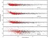 |
Fig. 20 Comparison of ERCSC and PCCS photometries at 143 GHz. Grey points correspond to common sources below | b | < 30° while red ones show the common ones for | b | > 30°. Dashed lines indicates the ± 10% uncertainty level. |
4.3. Comparison with the Planck ERCSC
The Early Release Compact Source Catalogue is a catalogue of high-reliability sources, both Galactic and extragalactic, detected over the full sky, in the first Planck all-sky survey. One of the primary goals of the ERCSC was to provide an early catalogue of sources for follow-up observations with existing facilities, in particular Herschel, while they were still in their cryogenic operational phase. The PCCS differs from the ERCSC both in the data and the philosophy.
The data used to build the ERCSC consisted of one complete survey and 60% of the second survey included in the maps. The data used for the PCCS consists of two complete surveys and 60% of the third survey. Moreover, our knowledge of the instruments has improved during this time, and this translates into a better calibration and quality of the maps, and better characterization of the beams (Planck Collaboration II 2014; Planck Collaboration VI 2014). The beam size and shapes are crucial to obtaining precise measurements of the flux densities. The change in beam sizes between those used for ERCSC and the present values used for the PCCS is ~2% in the LFI channels and ~8% in the HFI ones. Figure 20 shows a comparison at 143 GHz between the photometries from ERCSC and PCCS. Similar results are obtained for all the other channels.
The primary goal of the ERCSC, to provide a reliable catalogue, was successfully accomplished. The goal of the PCCS is to increase the completeness of the catalogue while maintaining a good global reliability (>80% by construction). This has led to the higher number of detections per channel (a factor 2–4 more sources) and better sensitivity achieved by the PCCS (see also Fig. 18 for a direct comparison between the PCCS and ERCSC completeness levels).
5. The PCCS: access, content and usage
The PCCS is available from the ESA Planck Legacy Archive3. The source lists contain 24 columns. The 857 GHz source list has six additional columns that consist of the band-filled aperture flux densities and associated uncertainties in the three adjacent frequency channels, 217–545 GHz, for each source detected at 857 GHz.
5.1. Catalogue content and usage
Detailed information about the catalogue content and format can be found in the Explanatory Supplement (Planck Collaboration Int. VII 2013) and in the FITS files headers. Here we summarize the most important features of the catalogues. The key columns in the catalogues are:
-
Source identification: NAME (string).
-
Position: GLON and GLAT contain the Galactic coordinates, and RA and DEC the equatorial coordinates (J2000).
-
Flux density: the four estimates of flux density (DETFLUX, APERFLUX, PSFFLUX, and GAUFLUX) in mJy, and their associated uncertainties (with the _ERR suffix).
-
Source extension: the EXTENDED flag is set to 1 if a source is extended. See the definition below.
-
Cirrus indicator: the CIRRUS_N column contains a cirrus indicator for the HFI channels. See the definition below.
-
External validation: the EXT_VAL contains a summary of the external validation for the LFI channels. See the definition below.
-
Identification with ERCSC: the ERCSC column indicates the name of the ERCSC counterpart, if there is one, at this channel.
A source is classified as extended if
 (3)where FWHMnom is the
nominal beam size for the selected channel and the quantity FWHMeff is the
geometric mean of the major and minor FWHM values from the Gaussian fit,
(3)where FWHMnom is the
nominal beam size for the selected channel and the quantity FWHMeff is the
geometric mean of the major and minor FWHM values from the Gaussian fit,
 (4)In the upper HFI bands,
sources that are extended tend to be associated with structure in the Galactic
interstellar medium although individual nearby galaxies are also extended sources as seen
by Planck (see Planck Collaboration XVI
2011). The choice of the threshold, 1.5 times the beam width, is motivated by the
accuracy with which source profiles can be measured from maps where the point spread
function is critically sampled (1.́7 pixel scale for a FHWM of ~4′). Naturally, faint sources for which the
Gaussian fitting failed do not have the EXTENDED flag set.
(4)In the upper HFI bands,
sources that are extended tend to be associated with structure in the Galactic
interstellar medium although individual nearby galaxies are also extended sources as seen
by Planck (see Planck Collaboration XVI
2011). The choice of the threshold, 1.5 times the beam width, is motivated by the
accuracy with which source profiles can be measured from maps where the point spread
function is critically sampled (1.́7 pixel scale for a FHWM of ~4′). Naturally, faint sources for which the
Gaussian fitting failed do not have the EXTENDED flag set.
Sources in the HFI channels have a cirrus indicator, CIRRUS_N. This is the number of sources detected at 857 GHz (using a uniform S/N threshold of 5) within a 1° radius of the source. Many 857 GHz detections at this S/N threshold in the Galactic region will be from cirrus knots, so it provides a useful indicator of the presence of cirrus.
The EXT_VAL column summarizes the cross-matching with external catalogues. For the LFI channels this is the set of radio catalogues used in the external validation (see Sect. 3.2). For HFI channels it is the catalogue extracted from the IRIS map (see Sect. 4.2). The EXT_VAL flag takes the value 0, 1, or 2:
-
0:
The source has no clear counterpart in any of the externalcatalogues and it has not been detected in otherPlanck channels.
-
1:
The source has no clear counterpart in any of the external catalogues, but it has been detected in other Planck channels.
-
2:
For the LFI channels, the source has a clear counterpart in the radio catalogues. For the HFI channels, the source either has a clear counterpart in the radio catalogues or in both the IRIS catalogue and all the higher Planck channels.
This flag provides valuable information about the reliability of individual sources: those flagged as EXT_VAL= 2 are already known, those with EXT_VAL = 1 have been detected in other Planck channels and are therefore potentially new sources, and those with EXT_VAL = 0 appear in only a single channel, and thus are more likely to be spurious. For the LFI channels, the matrix filters (Herranz et al. 2009) are used to determine whether a source has been detected in other Planck channels. For the HFI channels, the cross-matching is carried out a posteriori from the catalogues (see Sect. 4.2).
As described in Sect. 2.4, four measures of flux density are provided in units of mJy. For extended sources, both DETFLUX and PSFFLUX are likely to produce underestimates of the true source flux density. Furthermore, at faint flux densities corresponding to low S/N, the PSF and GAUSSIAN fits may fail. This would be represented either by a negative flux density or by a significant difference between the GAUFLUX and DETFLUX values. In general, for bright extended sources, we recommend using the GAUFLUX and GAUFLUX_ERR values although even these might be biased high if the source is located in a region of complex, diffuse foreground emission. Uncertainties in the flux density measured by each technique are reflected in the corresponding _ERR column.
The median positional uncertainty, given in Table 1, is only a statistical estimate for each band. Individual sources could have a larger positional offset depending on the local background rms and S/N. As this quantity has been obtained by comparison with external data sets it also takes into account any astrometric offset in the maps.
5.2. Cautionary notes on the use of catalogues
In this section, we remind readers of the preliminary nature of the PCCS and list some cautionary notes for users of the catalogue. The PCCS is based solely on the nine frequency maps derived from the nominal mission, which ended in November 2010. The HFI instrument continued to operate stably for another 14 months after the end of the nominal mission, and the LFI instrument is expected to complete an additional 5.4 full-sky surveys not included in the PCCS. Thus the PCCS is based on only a fraction of Planck data: approximately 1/3 in the case of LFI. The observations following the nominal mission will also allow for better control of systematic errors, which in turn is likely to improve the quality and accuracy of a later, more complete catalogue of Planck sources based on the entire mission. Our understanding of the instrument (effective beam size, for instance) has improved since the ERCSC was issued and will surely continue to improve. Likewise, we can expect further improvements in the use of ground-based and other facilities to validate properties of the catalogue, such as flux density scales. Note the improvement over validation efforts for the ERCSC, and the extension of external validation to 143 and 217 GHz (Sect. 3.2.2). It is also reasonable to expect further refinements in the algorithms used to detect sources and to measure their properties. Finally, the PCCS does not address, as future catalogues will, the issue of polarization.
As noted earlier, the aim of the PCCS is to provide as complete a list as possible of Planck sources with a reasonable degree of reliability. The criteria used to include or exclude candidate sources differ from channel to channel and in different parts of the sky; they also are based on different S/N levels. These differences were consequences of our desire to make the catalogue as complete as possible, yet maintain >80% reliability. These differences have to be taken into account when using the PCCS for statistical studies. On the other hand, we have endeavoured to ensure that the flux density scales of the various channel catalogues are consistent. They appear to be at the few percent level (see discusion in Planck Collaboration XXXI 2014).
We now turn to several specific cautions and comments for users of the PCCS.
Variability:
at radio frequencies, up to and including 217 GHz, many of the extragalactic sources are highly variable. A small fraction of them vary even on time scales of a few hours based on observed changes in the flux density as a source drifts through the different Planck horns (Planck Collaboration II 2014; Planck Collaboration VI 2014). Follow-up observations of these sources might show significant differences in flux density compared to the values in the Planck data products. Although the maps used for the PCCS are based on 2.6 sky coverages, the PCCS provides only a single average flux density estimate over all Planck data samples that were included in the maps and does not contain any measure of the variability of the sources from survey to survey.
Contamination from CO:
at infrared/submillimetre frequencies (100 GHz and above), the Planck bandpasses straddle energetically significant CO lines. The effect is the greatest at 100 GHz, where the line contributes strongly to the flux densities of Galactic sources. Aperture photometry at PCCS candidate locations using the type-3 CO map derived from Planck component separation (Planck Collaboration XIII 2014) shows that 91% of detections within the 85% Galactic dust mask have CO contamination of their APERFLUX estimates at the level of 20% or higher. Outside this mask, this contamination drops to 6%. Follow-up observations of these Galactic sources, especially those associated with Galactic star-forming regions, at a similar frequency but different bandpass, should correct for the contribution of line emission to the measured continuum flux density of the source.
Photometry:
each source has multiple estimates of flux density, DETFLUX, APERFLUX, GAUFLUX and PSFFLUX, as defined above. The appropriate photometry to be used depends on the nature of the source. For sources that are unresolved at the spatial resolution of Planck, APERFLUX and DETFLUX are most appropriate. Even in this regime, PSF or Gaussian fits of faint sources fail and consequently these have a PSFFLUX/GAUFLUX value of NaN (“Not a Number”). For bright resolved sources, GAUFLUX might be most appropriate although GAUFLUX appears to overestimate the flux density of the sources close to the Galactic plane due to an inability to fit for the contribution of the Galactic background at the spatial resolution of the data. For the 353–857 GHz channels, the complex nature of the diffuse emission and the relative undersampling of the beam produces a bias in DETFLUX, we therefore recommend that APERFLUX is used instead (see Fig. 14).
Calibration:
the absolute calibration uncertainties of Planck are <1% for 30–217 GHz and are <1.2% at 353 GHz. For 545 and 857 GHz, the absolute calibration uncertainty is <10% (Planck Collaboration II 2014; Planck Collaboration V 2014; Planck Collaboration VI 2014; Planck Collaboration VIII 2014). For these two channels the calibration uncertainty is an appreciable systematic error on the photometry, which is not included in the internal validation (as it was not simulated) or the external comparison with Herschel photometry (see Sect. 3.2.3) as the inter-calibration between HFI and SPIRE was corrected prior to comparison.
Colour correction:
the flux density estimates have not been colour corrected. Colour corrections are described in Planck Collaboration II (2014) and Planck Collaboration VI (2014). The typical amplitude of the correction is below 4% for synchrotron-like spectra in the LFI channels and below 15% for thermal emission in the HFI channels. Colour corrections can be calculated using Planck unit conversion and colour correction software (UC_CC), included in the data release (Planck Collaboration IX 2014), which uses the instrumental bandpasses (Planck Collaboration Int. VII 2013).
Cirrus/ISM:
a significant fraction of the sources detected in the upper HFI bands could be associated with Galactic interstellar medium features or cirrus. The value of CIRRUS_N in the catalogue can be used to flag sources that might be clustered together and thereby associated with ISM structure. Candidate ISM features can also be selected by choosing objects with EXTENDED =1 although nearby Galactic and extragalactic sources that are extended at Planck spatial resolution will meet this criterion too. The 857 GHz brightness proxy described in Sect. 3.4 can also be used as indicator of cirrus contamination.
6. Conclusions
The PCCS lists sources extracted from the Planck nominal mission data in each of its nine frequency bands. By construction its reliability is >80% and a special effort was made to use simple selection procedures in order to facilitate statistical analyses. With a common detection method for all the channels and the additional three photometric estimates, spectral analysis can also be performed safely. The deeper completeness levels and, as a consequence, the higher number of sources compared with the ERCSC, will allow the extension of previous studies to more sources and to fainter flux densities. The PCCS is the natural evolution of the ERCSC, but both lack polarization and multi-frequency information. Future releases will take advantage of the full mission data and they will contain information on properties of sources not available in this release, including polarization and variability, and association of sources detected in different bands.
This paper describes the construction and properties of this preliminary catalogue. We have not attempted to exploit the PCCS for science purposes, preferring instead to leave this to future papers and to the wider community.
Planck (http://www.esa.int/Planck) is a project of the European Space Agency (ESA) with instruments provided by two scientific consortia funded by ESA member states (in particular the lead countries France and Italy), with contributions from NASA (USA) and telescope reflectors provided by a collaboration between ESA and a scientific consortium led and funded by Denmark.
Acknowledgments
The development of Planck has been supported by: ESA; CNES and CNRS/INSU-IN2P3-INP (France); ASI, CNR, and INAF (Italy); NASA and DoE (USA); STFC and UKSA (UK); CSIC, MICINN, JA and RES (Spain); Tekes, AoF and CSC (Finland); DLR and MPG (Germany); CSA (Canada); DTU Space (Denmark); SER/SSO (Switzerland); RCN (Norway); SFI (Ireland); FCT/MCTES (Portugal); and PRACE (EU). A description of the Planck Collaboration and a list of its members, including the technical or scientific activities in which they have been involved, can be found at http://www.sciops.esa.int/index.php?project=planck&page=Planck_Collaboration. This research has made use of Aladin. We are deeply grateful to Rick Perley and the U.S. National Radio Astronomy Observatory for participating in the joint Planck-VLA observations. We also thank Steve Eales and the H-ATLAS team (Eales et al, 2010 PASP 122 499E) for sharing their SPIRE catalogs prior to publication, allowing a comparison of flux densities between HFI and SPIRE.
References
- AMI Consortium, Perrott, Y. C., Green, D. A., et al. 2012, MNRAS, 421, L6 [NASA ADS] [CrossRef] [Google Scholar]
- André, P., Men’shchikov, A., Bontemps, S., et al. 2010, A&A, 518, L102 [NASA ADS] [CrossRef] [EDP Sciences] [Google Scholar]
- Beichman, C. A., Neugebauer, G., Habing, H. J., Clegg, P. E., & Chester, T. J., 1988, Infrared astronomical satellite (IRAS) catalogs and atlases, Vol. 1: Explanatory supplement, 1 [Google Scholar]
- Bennett, C. L., Larson, D., Weiland, J. L., et al. 2013, ApJS, 208, 20 [Google Scholar]
- Bonaldi, A., Bonavera, L., Massardi, M., & De Zotti, G. 2013, MNRAS, 428, 1845 [NASA ADS] [CrossRef] [Google Scholar]
- Bonavera, L., Massardi, M., Bonaldi, A., et al. 2011, MNRAS, 416, 559 [NASA ADS] [Google Scholar]
- Boselli, A., Eales, S., Cortese, L., et al. 2010, PASP, 122, 261 [NASA ADS] [CrossRef] [Google Scholar]
- Chen, X., Rachen, J. P., López-Caniego, M., et al. 2013, A&A, 553, A107 [NASA ADS] [CrossRef] [EDP Sciences] [Google Scholar]
- Clements, D. L., Rigby, E., Maddox, S., et al. 2010, A&A, 518, L8 [NASA ADS] [CrossRef] [EDP Sciences] [Google Scholar]
- Clemens, M. S., Negrello, M., De Zotti, G., et al. 2013, MNRAS, 433, 695 [NASA ADS] [CrossRef] [Google Scholar]
- Condon, J. J. 1974, ApJ, 188, 279 [NASA ADS] [CrossRef] [Google Scholar]
- Crawford, T. M., Switzer, E. R., Holzapfel, W. L., et al. 2010, ApJ, 718, 513 [NASA ADS] [CrossRef] [Google Scholar]
- Dale, D. A., Bendo, G. J., Engelbracht, C. W., et al. 2005, ApJ, 633, 857 [NASA ADS] [CrossRef] [Google Scholar]
- Davies, J. I., Bianchi, S., Baes, M., et al. 2013, MNRAS, 428, 834 [NASA ADS] [CrossRef] [Google Scholar]
- de Zotti, G., Ricci, R., Mesa, D., et al. 2005, A&A, 431, 893 [NASA ADS] [CrossRef] [EDP Sciences] [Google Scholar]
- Delabrouille, J., Betoule, M., Melin, J.-B., et al. 2013, A&A, 553, A96 [NASA ADS] [CrossRef] [EDP Sciences] [Google Scholar]
- Dole, H., Lagache, G., & Puget, J.-L. 2003, ApJ, 585, 617 [NASA ADS] [CrossRef] [Google Scholar]
- Dole, H., Lagache, G., Puget, J.-L., et al. 2006, A&A, 451, 417 [NASA ADS] [CrossRef] [EDP Sciences] [MathSciNet] [Google Scholar]
- Dunne, L., Eales, S., Edmunds, M., et al. 2000, MNRAS, 315, 115 [NASA ADS] [CrossRef] [Google Scholar]
- Eales, S., Dunne, L., Clements, D., et al. 2010, PASP, 122, 499 [NASA ADS] [CrossRef] [Google Scholar]
- Eddington, Sir, A. S. 1940, MNRAS, 100, 354 [NASA ADS] [CrossRef] [Google Scholar]
- Franceschini, A., Toffolatti, L., Danese, L., & de Zotti, G. 1989, ApJ, 344, 35 [NASA ADS] [CrossRef] [Google Scholar]
- Fu, H., Jullo, E., Cooray, A., et al. 2012, ApJ, 753, 134 [NASA ADS] [CrossRef] [Google Scholar]
- González-Nuevo, J., Argüeso, F., López-Caniego, M., et al. 2006, MNRAS, 369, 1603 [NASA ADS] [CrossRef] [Google Scholar]
- González-Nuevo, J., Massardi, M., Argüeso, F., et al. 2008, MNRAS, 384, 711 [NASA ADS] [CrossRef] [Google Scholar]
- Górski, K. M., Hivon, E., Banday, A. J., et al. 2005, ApJ, 622, 759 [NASA ADS] [CrossRef] [Google Scholar]
- Gregory, P. C., Scott, W. K., Douglas, K., & Condon, J. J. 1996, ApJS, 103, 427 [NASA ADS] [CrossRef] [Google Scholar]
- Griffin, M. J., Abergel, A., Abreu, A., et al. 2010, A&A, 518, L3 [Google Scholar]
- Hacking, P., Condon, J. J., & Houck, J. R. 1987, ApJ, 316, L15 [NASA ADS] [CrossRef] [Google Scholar]
- Healey, S. E., Romani, R. W., Taylor, G. B., et al. 2007, ApJS, 171, 61 [NASA ADS] [CrossRef] [Google Scholar]
- Helou, G., & Beichman, C. A. 1990, in Liege International Astrophysical Colloquia 29, ed. B. Kaldeich, 117 [Google Scholar]
- Herranz, D., & Sanz, J. L. 2008, IEEE J. Select. Topics Signal Process., 2, 727 [Google Scholar]
- Herranz, D., López-Caniego, M., Sanz, J. L., & González-Nuevo, J. 2009, MNRAS, 394, 510 [NASA ADS] [CrossRef] [Google Scholar]
- Herranz, D., González-Nuevo, J., Clements, D. L., et al. 2013, A&A, 549, A31 [NASA ADS] [CrossRef] [EDP Sciences] [Google Scholar]
- Kennicutt, R. C., Calzetti, D., Aniano, G., et al. 2011, PASP, 123, 1347 [NASA ADS] [CrossRef] [Google Scholar]
- Kurinsky, N., Sajina, A., Partridge, B., et al. 2013, A&A, 549, A133 [NASA ADS] [CrossRef] [EDP Sciences] [Google Scholar]
- Lanz, L. F., Herranz, D., López-Caniego, M., et al. 2013, MNRAS, 428, 3048 [NASA ADS] [CrossRef] [Google Scholar]
- Leach, S. M., Cardoso, J.-F., Baccigalupi, C., et al. 2008, A&A, 491, 597 [NASA ADS] [CrossRef] [EDP Sciences] [Google Scholar]
- López-Caniego, M., Herranz, D., González-Nuevo, J., et al. 2006, MNRAS, 370, 2047 [NASA ADS] [CrossRef] [Google Scholar]
- López-Caniego, M., González-Nuevo, J., Herranz, D., et al. 2007, ApJS, 170, 108 [NASA ADS] [CrossRef] [Google Scholar]
- Marsden, D., Gralla, M., Marriage, T. A., et al. 2014, MNRAS, 439, 1556 [NASA ADS] [CrossRef] [Google Scholar]
- Massardi, M., López-Caniego, M., González-Nuevo, J., et al. 2009, MNRAS, 392, 733 [NASA ADS] [CrossRef] [Google Scholar]
- Massardi, M., Bonaldi, A., Bonavera, L., et al. 2011, MNRAS, 415, 1597 [NASA ADS] [CrossRef] [Google Scholar]
- Mitra, S., Rocha, G., Górski, K. M., et al. 2011, ApJS, 193, 5 [NASA ADS] [CrossRef] [Google Scholar]
- Miville-Deschênes, M.-A. & Lagache, G. 2005, ApJS, 157, 302 [NASA ADS] [CrossRef] [Google Scholar]
- Mocanu, L. M., Crawford, T. M., Vieira, J. D., et al. 2013, ApJ, 779, 61 [NASA ADS] [CrossRef] [Google Scholar]
- Murphy, T., Sadler, E. M., Ekers, R. D., et al. 2010, MNRAS, 402, 2403 [NASA ADS] [CrossRef] [Google Scholar]
- Negrello, M., Magliocchetti, M., Moscardini, L., et al. 2004, MNRAS, 352, 493 [NASA ADS] [CrossRef] [Google Scholar]
- Negrello, M., Clemens, M., Gonzalez-Nuevo, J., et al. 2013, MNRAS, 429, 1309 [NASA ADS] [CrossRef] [Google Scholar]
- Perley, R. A., & Butler, B. J. 2013, ApJS, 204, 19 [NASA ADS] [CrossRef] [Google Scholar]
- Planck Collaboration VII. 2011, A&A, 536, A7 [NASA ADS] [CrossRef] [EDP Sciences] [Google Scholar]
- Planck Collaboration XIII. 2011, A&A, 536, A13 [NASA ADS] [CrossRef] [EDP Sciences] [Google Scholar]
- Planck Collaboration XIV. 2011, A&A, 536, A14 [NASA ADS] [CrossRef] [EDP Sciences] [Google Scholar]
- Planck Collaboration XV. 2011, A&A, 536, A15 [NASA ADS] [CrossRef] [EDP Sciences] [Google Scholar]
- Planck Collaboration XVI. 2011, A&A, 536, A16 [NASA ADS] [CrossRef] [EDP Sciences] [Google Scholar]
- Planck Collaboration XIX. 2011, A&A, 536, A19 [NASA ADS] [CrossRef] [EDP Sciences] [Google Scholar]
- Planck Collaboration XXIII. 2011, A&A, 536, A23 [NASA ADS] [CrossRef] [EDP Sciences] [Google Scholar]
- Planck Collaboration Int. VII. 2013, A&A, 550, A133 [NASA ADS] [CrossRef] [EDP Sciences] [Google Scholar]
- Planck Collaboration 2013, The Explanatory Supplement to the Planck 2013 results, http://www.sciops.esa.int/wikiSI/planckpla/index.php?title=Main_Page (ESA) [Google Scholar]
- Planck Collaboration I. 2014, A&A, 571, A1 [NASA ADS] [CrossRef] [EDP Sciences] [Google Scholar]
- Planck Collaboration II. 2014, A&A, 571, A2 [NASA ADS] [CrossRef] [EDP Sciences] [Google Scholar]
- Planck Collaboration III. 2014, A&A, 571, A3 [NASA ADS] [CrossRef] [EDP Sciences] [Google Scholar]
- Planck Collaboration IV. 2014, A&A, 571, A4 [NASA ADS] [CrossRef] [EDP Sciences] [Google Scholar]
- Planck Collaboration V. 2014, A&A, 571, A5 [NASA ADS] [CrossRef] [EDP Sciences] [Google Scholar]
- Planck Collaboration VI. 2014, A&A, 571, A6 [NASA ADS] [CrossRef] [EDP Sciences] [Google Scholar]
- Planck Collaboration VII. 2014, A&A, 571, A7 [NASA ADS] [CrossRef] [EDP Sciences] [Google Scholar]
- Planck Collaboration VIII. 2014, A&A, 571, A8 [NASA ADS] [CrossRef] [EDP Sciences] [Google Scholar]
- Planck Collaboration IX. 2014, A&A, 571, A9 [NASA ADS] [CrossRef] [EDP Sciences] [Google Scholar]
- Planck Collaboration X. 2014, A&A, 571, A10 [NASA ADS] [CrossRef] [EDP Sciences] [Google Scholar]
- Planck Collaboration XI. 2014, A&A, 571, A11 [NASA ADS] [CrossRef] [EDP Sciences] [Google Scholar]
- Planck Collaboration XII. 2014, A&A, 571, A12 [NASA ADS] [CrossRef] [EDP Sciences] [Google Scholar]
- Planck Collaboration XIII. 2014, A&A, 571, A13 [NASA ADS] [CrossRef] [EDP Sciences] [Google Scholar]
- Planck Collaboration XIV. 2014, A&A, 571, A14 [NASA ADS] [CrossRef] [EDP Sciences] [Google Scholar]
- Planck Collaboration XV. 2014, A&A, 571, A15 [NASA ADS] [CrossRef] [EDP Sciences] [Google Scholar]
- Planck Collaboration XVI. 2014, A&A, 571, A16 [NASA ADS] [CrossRef] [EDP Sciences] [Google Scholar]
- Planck Collaboration XVII. 2014, A&A, 571, A17 [NASA ADS] [CrossRef] [EDP Sciences] [Google Scholar]
- Planck Collaboration XVIII. 2014, A&A, 571, A18 [NASA ADS] [CrossRef] [EDP Sciences] [Google Scholar]
- Planck Collaboration XIX. 2014, A&A, 571, A19 [NASA ADS] [CrossRef] [EDP Sciences] [Google Scholar]
- Planck Collaboration XX. 2014, A&A, 571, A20 [NASA ADS] [CrossRef] [EDP Sciences] [Google Scholar]
- Planck Collaboration XXI. 2014, A&A, 571, A21 [NASA ADS] [CrossRef] [EDP Sciences] [Google Scholar]
- Planck Collaboration XXII. 2014, A&A, 571, A22 [NASA ADS] [CrossRef] [EDP Sciences] [Google Scholar]
- Planck Collaboration XXIII. 2014, A&A, 571, A23 [NASA ADS] [CrossRef] [EDP Sciences] [MathSciNet] [PubMed] [Google Scholar]
- Planck Collaboration XXIV. 2014, A&A, 571, A24 [NASA ADS] [CrossRef] [EDP Sciences] [Google Scholar]
- Planck Collaboration XXV. 2014, A&A, 571, A25 [NASA ADS] [CrossRef] [EDP Sciences] [Google Scholar]
- Planck Collaboration XXVI. 2014, A&A, 571, A26 [NASA ADS] [CrossRef] [EDP Sciences] [Google Scholar]
- Planck Collaboration XXVII. 2014, A&A, 571, A27 [NASA ADS] [CrossRef] [EDP Sciences] [Google Scholar]
- Planck Collaboration XXVIII. 2014, A&A, 571, A28 [NASA ADS] [CrossRef] [EDP Sciences] [Google Scholar]
- Planck Collaboration XXIX. 2014, A&A, 571, A29 [NASA ADS] [CrossRef] [EDP Sciences] [Google Scholar]
- Planck Collaboration XXX. 2014, A&A, 571, A30 [NASA ADS] [CrossRef] [EDP Sciences] [Google Scholar]
- Planck Collaboration XXXI. 2014, A&A, 571, A31 [NASA ADS] [CrossRef] [EDP Sciences] [Google Scholar]
- Planck Collaboration Int. XIV. 2014, A&A, 564, A45 [NASA ADS] [CrossRef] [EDP Sciences] [Google Scholar]
- Rigby, E. E., Maddox, S. J., Dunne, L., et al. 2011, MNRAS, 415, 2336 [NASA ADS] [CrossRef] [Google Scholar]
- Toffolatti, L., Argueso Gomez, F., de Zotti, G., et al. 1998, MNRAS, 297, 117 [NASA ADS] [CrossRef] [Google Scholar]
Appendix A: Photometry
This appendix describes in detail the photometry methods used in the PCCS.
Appendix A.1: Aperture photometry
The aperture photometry is evaluated by centring a circular aperture on the position of
the source. An annulus around this aperture is used to evaluate the background. In the
absence of noise, the observed flux density of the source, Sobs, may be
written as: 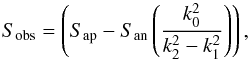 (A.1)where k0 is the
radius of the aperture, k1 and k2 are the
inner and outer radii of the annulus, and, Sap and San are the
flux densities of the source in the aperture and annulus. Both Sap and
Sann may be written in terms of the true
flux density of the source, Strue. This gives the following
relationship between the observed and true flux densities of the source:
(A.1)where k0 is the
radius of the aperture, k1 and k2 are the
inner and outer radii of the annulus, and, Sap and San are the
flux densities of the source in the aperture and annulus. Both Sap and
Sann may be written in terms of the true
flux density of the source, Strue. This gives the following
relationship between the observed and true flux densities of the source: 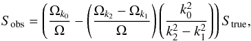 (A.2)where
Ω is the solid angle of
the beam, and Ωk0, Ωk1, and Ωk2
are the beam solid angles out to the radii of k0, k1 and
k2. This provides the correction factor
to be applied to the observed flux density, which accounts for both the flux density of
the source missing from the aperture and that removed through background subtraction.
(A.2)where
Ω is the solid angle of
the beam, and Ωk0, Ωk1, and Ωk2
are the beam solid angles out to the radii of k0, k1 and
k2. This provides the correction factor
to be applied to the observed flux density, which accounts for both the flux density of
the source missing from the aperture and that removed through background subtraction.
Assuming a circularly symmetric Gaussian beam and that k0,
k1 and k2 are given
in units of the FWHM, Eq. (A.2) may be
written as: 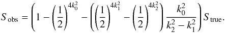 (A.3)We used a radius of
1 FWHM for the aperture, k0 = 1, and the annulus is located
immediately outside of the aperture and has a width of 1 FWHM, k1 = 1 and
k2 =
2.
(A.3)We used a radius of
1 FWHM for the aperture, k0 = 1, and the annulus is located
immediately outside of the aperture and has a width of 1 FWHM, k1 = 1 and
k2 =
2.
The beams however are not exactly Gaussian so the effective FWHM is used to determine
the radii of the aperture and annulus, and the correction factor is evaluated using:
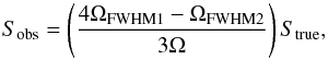 (A.4)where
ΩFWHM1 and
ΩFWHM2 are the
beam solid angles within radii of 1 and 2 times the effective FWHM.
(A.4)where
ΩFWHM1 and
ΩFWHM2 are the
beam solid angles within radii of 1 and 2 times the effective FWHM.
The noise level per pixel is estimated from the variance of the pixels that lie in the annulus, hence the uncertainties in the estimates of the background and the flux density within the aperture may be evaluated, allowing the uncertainty on Sobs to be calculated. The diffuse sky emission is a source of uncertainty in the photometry, thus it contributes a component to the “noise” that is correlated between pixels. Given that the exact degree of correlation is not known and is likely to vary with position on the sky, a correction factor to account for the correlated noise is evaluated by performing aperture photometry nearby, in regions without detected sources. Its value is such that it scales the residuals normalized by the uncertainties to a Gaussian of unit variance.
Appendix A.2: PSF photometry
The PSF photometry is obtained by fitting a model of the PSF to the map at the position
of the source. The PSF is obtained from the effective beam (Planck Collaboration II 2014; Planck
Collaboration VI 2014). The model of the source is
 (A.5)where P is the PSF
at the position of the source, A is the amplitude of the source and
C is a
the (constant) background. The best-fit values of the parameters β =
(A,C) are found by minimising the χ2 between the
model and the data, d,
(A.5)where P is the PSF
at the position of the source, A is the amplitude of the source and
C is a
the (constant) background. The best-fit values of the parameters β =
(A,C) are found by minimising the χ2 between the
model and the data, d,  (A.6)where
N is the covariance matrix
of the noise. The noise is assumed to be uncorrelated between pixels and proportional to
the inverse of the number of hits in each pixel. The overall normalization of the noise
is adjusted by setting χ2 = 1 at the best-fit value of the
parameters. This has the effect of inflating the uncertainties to account for any
mismatch between the modelled PSF and the true shape of the source in the map. The
uncertainties on the parameters are computed from the curvature of the χ2. The
best-fit amplitude and its uncertainty are converted to units of flux density using the
area of the PSF.
(A.6)where
N is the covariance matrix
of the noise. The noise is assumed to be uncorrelated between pixels and proportional to
the inverse of the number of hits in each pixel. The overall normalization of the noise
is adjusted by setting χ2 = 1 at the best-fit value of the
parameters. This has the effect of inflating the uncertainties to account for any
mismatch between the modelled PSF and the true shape of the source in the map. The
uncertainties on the parameters are computed from the curvature of the χ2. The
best-fit amplitude and its uncertainty are converted to units of flux density using the
area of the PSF.
Appendix A.3: Gaussian fit photometry
The Gaussian fit photometry is obtained by fitting a 2-dimensional Gaussian to the map
at the position of the source. The model consists of a elliptical Gaussian centred at
the position of the source plus a linear background,
![\appendix \setcounter{section}{1} \begin{equation} m(\vec{x}) = A \exp\left[-\vec{x}^{\rm T}\tens{Q}^{-1}\vec{x}/2\right] + \vec{B}\cdot\vec{x} + C , \end{equation}](/articles/aa/full_html/2014/11/aa21524-13/aa21524-13-eq122.png) (A.7)where A is the amplitude of the
source, Q is the covariance
matrix of the elliptical Gaussian profile, and B and
C are the
background parameters. It is assumed that the source is at the origin of the coordinates
x. The components of Q can be expressed as a function of the
semi-axes a
and b, and
an orientation angle θ as
(A.7)where A is the amplitude of the
source, Q is the covariance
matrix of the elliptical Gaussian profile, and B and
C are the
background parameters. It is assumed that the source is at the origin of the coordinates
x. The components of Q can be expressed as a function of the
semi-axes a
and b, and
an orientation angle θ as
 (A.8)where R
is the rotation matrix,
(A.8)where R
is the rotation matrix, ![\appendix \setcounter{section}{1} \begin{equation} \textbf{R}=\left[ \begin{array}{cc} \cos\theta & -\sin\theta \\ \sin\theta & \cos\theta \end{array} \right] , \end{equation}](/articles/aa/full_html/2014/11/aa21524-13/aa21524-13-eq130.png) (A.9)and
(A.9)and
![\appendix \setcounter{section}{1} \begin{equation} \textbf{C}^{-1}=\left[ \begin{array}{cc} 1/a^2 & 0 \\ 0 & 1/b^2 \end{array} \right] . \end{equation}](/articles/aa/full_html/2014/11/aa21524-13/aa21524-13-eq131.png) (A.10)There are seven
parameters to fit
(A.10)There are seven
parameters to fit ![\appendix \setcounter{section}{1} \begin{equation} \beta = [A, B_1, B_2, C, a, b, \theta] . \end{equation}](/articles/aa/full_html/2014/11/aa21524-13/aa21524-13-eq132.png) (A.11)The model is
fitted to the data by minimising the χ2 (A.6) between a pixelized version of the model m and the
data d. The uncertainties on the parameters
are given by the diagonal elements of the covariance matrix of the fit. Assuming that
the elliptical Gaussian model is a good approximation to the real source profile, the
amplitude of the source and its uncertainty are converted to units of flux density using
the area of the Gaussian.
(A.11)The model is
fitted to the data by minimising the χ2 (A.6) between a pixelized version of the model m and the
data d. The uncertainties on the parameters
are given by the diagonal elements of the covariance matrix of the fit. Assuming that
the elliptical Gaussian model is a good approximation to the real source profile, the
amplitude of the source and its uncertainty are converted to units of flux density using
the area of the Gaussian.
All Tables
Native photometry (DETFLUX) bias (mean multiplicative), photometric recovery uncertainty, and median radial position uncertainty from the internal validation, all calculated in the extragalactic zone.
All Figures
|
Fig. 1 Sky distribution of the PCCS sources at three different channels: 30 GHz (pink circles); 143 GHz (magenta circles); and 857 GHz (green circles). The dimension of the circles is related to the brightness of the sources and the beam size of each channel. The figure is a full-sky Aitoff projection with the Galactic equator horizontal; longitude increases to the left with the Galactic centre in the centre of the map. |
| In the text | |
|
Fig. 2 The Galactic and extragalactic zones used to define the S/N thresholds to meet the reliability target. The figure is a full-sky Mollweide projection. See text for further details. |
| In the text | |
|
Fig. 3 Comparison of the APERFLUX, PSFFLUX and GAUFLUX flux density estimates with the DETFLUX ones for the 100 GHz catalogue, (S − SDETFLUX) /SDETFLUX. Grey points correspond to sources below | b | < 5° while red ones show the ones for | b | > 5°. Dashed lines indicates the ± 10% uncertainty level. |
| In the text | |
|
Fig. 4 Test of internal consistency between the two implementations of the MHW pipeline at 30 GHz for | b | > 30°. Top panel: cumulative percentage of sources detected by both methods. Middle panel: cumulative percentage of sources detected by only one of the methods. Bottom panel: comparison of the recovered flux densities (DETFLUX). |
| In the text | |
|
Fig. 5 Galactic dust masks used to estimate completeness and reliability for some of the HFI channels. The unmasked zones correspond to sky fractions of 65% and 85%. The figure is a full-sky Mollweide projection. See text for further details. |
| In the text | |
|
Fig. 6 Results of the internal validation for HFI channels. The quantities plotted are (left) completeness per bin, (middle) a map of sensitivity (the 50% completeness threshold in flux density), and (right) cumulative reliability as a function of S/N. The black curves in completeness are for the extragalactic zone described in Sect. 2.3. The red curves in completeness are for smaller masks used for the reliability estimation (if the extragalactic zone was not used). See text for discussion of the limitations of the injection reliability estimate used for 353 GHz and above. |
| In the text | |
|
Fig. 7 Example distributions of photometric recovery (left) and positional error (right) for 143 GHz (top row) and 857 GHz (bottom row). |
| In the text | |
|
Fig. 8 External validation summary (completeness and number of non-matched sources) of the 30, 44, and 70 GHz channels. |
| In the text | |
|
Fig. 9 Comparison between the PACO sample (Massardi et al. 2011; Bonavera et al. 2011; Bonaldi et al. 2013) and the extrapolated, colour-corrected PCCS flux densities (DETFLUX) at 32 (left) and 40 GHz (right). The multiple PACO observations of each source have been averaged to a single flux density and therefore the uncertainties reflect the variability of the sources instead of the actual flux density accuracy of the measurements (a few mJy). |
| In the text | |
|
Fig. 10 Comparison between the Metsähovi and the colour-corrected PCCS flux densities (DETFLUX) interpolated to 37 GHz using 30 and 44 GHz Planck data (left) and 30 and 70 GHz data (right). The multiple observations of each source have been averaged to a single flux density and therefore the uncertainties reflect the variability of the sources instead of the actual flux density accuracy of the measurements (a few mJy). |
| In the text | |
|
Fig. 11 Planck flux densities for bright sources observed within a month of VLA observations at that frequency. Planck values (APERFLUX) were colour-corrected and interpolated to ~28 GHz (left) and ~43 GHz (right). |
| In the text | |
|
Fig. 12 Comparison between ACT and Planck measurements (DETFLUX; colour-corrected). Left panel: Planck measurements were extrapolated to 148 GHz. Planck flux densities are on average 1% fainter (or ACT’s brighter). The uncertainty in the slope is 0.025 = 2.5%. Right panel: Planck measurements were extrapolated to 218 GHz.The slope is 1.033: Planck flux densities are high (or ACT’s low) by 3.3 ± 3.4% on average. |
| In the text | |
|
Fig. 13 Comparison between SCUBA and Planck flux densities at 353 GHz. All four PCCS flux densities estimates are shown, from left to right, APERFLUX, PSFFLUX, GAUFLUX, and DETFLUX. A colour correction of 0.898 has been applied to the Planck flux densities. The vertical dashed line shows the 90% completeness level of the PCCS. The diagonals show the line of equality between the flux densities. |
| In the text | |
|
Fig. 14 Comparison between Herschel and Planck flux densities at 545 GHz (top) and 857 GHz (bottom). All four PCCS flux densities estimates are shown, from left to right, APERFLUX, PSFFLUX, GAUFLUX, and DETFLUX. The Herschel 500 μm data have been extrapolated to 550 μm (545 GHz) assuming a spectral index of 2.7. The vertical dashed line shows the 90% completeness level of the PCCS. The diagonals show the line of equality between the flux densities. |
| In the text | |
|
Fig. 15 Cumulative reliability (top panel) and differential completeness (bottom panel) of the HFI–MHW and LFI–MHW catalogues at 70 GHz as determined by their respective internal and external validation procedures. |
| In the text | |
|
Fig. 16 The Polaris field observed by Planck (top) and Herschel (bottom) at 857 GHz (350 μm). Structures that appear to be compact sources to Planck, shown with yellow circles, are revealed to be cirrus knots when observed at higher resolution. They are located in regions with bright backgrounds, which provides a proxy for identifying them. The declination grid has spacing of 30 arc-min. |
| In the text | |
|
Fig. 17 Power spectra of six fields observed by both Planck (red) and Herschel (black). Fits to the spectra are shown in blue. There is a good agreement between Planck and Herschel in the common multipole range (typically ℓ< 3000). Fields are, from top to bottom: (a) Aquila; (b) Polaris; (c) Spider; (d) Draco; (e) Gama; (f) FLS; and (g) XMM-LSS. No real Galactic sources are expected in fields (b)–(g), only extragalactic sources (correlated and Poisson components) and cirrus at larger angular scales. Real Galactic sources are detected, however, in (a) (André et al. 2010): the power spectrum is orders of magnitude above the other fields, demonstrating the need to separate the Galactic from extragalactic zones, and the use of the background brightness as a proxy to estimate the cirrus contamination. |
| In the text | |
|
Fig. 18 The PCCS completeness level outside the Galactic plane (see Table 1) is shown relative to other wide area surveys. The ERCSC completeness levels have been obtained from Planck Collaboration XIII (2011) up to 70 GHz and Planck Collaboration Int. VII (2013) for the other channels, while the WMAP ones are from González-Nuevo et al. (2008) up to 41 GHz and Lanz et al. (2013) for 61 and 94 GHz. The sensitivity levels for Herschel SPIRE and PACS instruments are from Clements et al. (2010) and Rigby et al. (2011), respectively. The other wide area surveys shown as a comparison are: GB6 (Gregory et al. 1996), CRATES (Healey et al. 2007), AT20G (Murphy et al. 2010), PACO (Bonavera et al. 2011), SPT (Mocanu et al. 2013), ACT (Marsden et al. 2014) and IRAS (Beichman et al. 1988). |
| In the text | |
|
Fig. 19 Spectral indices of PCCS sources matched between contiguous channels with | b | > 30°. Each panel also shows the number of sources and the fraction with α> 1. The median values are indicated by vertical dashed lines. |
| In the text | |
|
Fig. 20 Comparison of ERCSC and PCCS photometries at 143 GHz. Grey points correspond to common sources below | b | < 30° while red ones show the common ones for | b | > 30°. Dashed lines indicates the ± 10% uncertainty level. |
| In the text | |
Current usage metrics show cumulative count of Article Views (full-text article views including HTML views, PDF and ePub downloads, according to the available data) and Abstracts Views on Vision4Press platform.
Data correspond to usage on the plateform after 2015. The current usage metrics is available 48-96 hours after online publication and is updated daily on week days.
Initial download of the metrics may take a while.