| Issue |
A&A
Volume 694, February 2025
|
|
|---|---|---|
| Article Number | A185 | |
| Number of page(s) | 22 | |
| Section | Catalogs and data | |
| DOI | https://doi.org/10.1051/0004-6361/202452811 | |
| Published online | 12 February 2025 | |
MOCKA – A PLATO mock asteroseismic catalogue: Simulations for gravity-mode oscillators
1
Institute for Astronomy, KU Leuven,
Celestijnenlaan 200D bus 2401,
3001
Leuven,
Belgium
2
Department of Astrophysics, IMAPP, Radboud University Nijmegen,
PO Box 9010,
6500 GL
Nijmegen,
The Netherlands
3
Max Planck Institute for Astronomy,
Koenigstuhl 17,
69117
Heidelberg,
Germany
4
Sub-department of Astrophysics, Department of Physics, University of Oxford,
Oxford
OX1 3RH,
UK
5
HUN-REN CSFK Konkoly Observatory, MTA Centre of Excellence,
Konkoly Thege Miklós út 15-17,
1121
Budapest,
Hungary
6
ELTE Eötvös Loránd University, Institute of Physics and Astronomy,
1117 Pázmány Péter sétány 1/A,
Budapest,
Hungary
7
Department of Astrophysical Sciences, Princeton University,
4 Ivy Lane,
Princeton,
NJ
08544,
USA
8
School of Mathematics, Statistics and Physics, Newcastle University,
Newcastle upon Tyne,
NE1 7RU,
UK
9
Sydney Institute for Astronomy, School of Physics, University of Sydney,
Sydney,
NSW 2006,
Australia
★ Corresponding author; nicholas.jannsen@kuleuven.be
Received:
30
October
2024
Accepted:
14
December
2024
Context. With the PLAnetary Transits and Oscillation of stars (PLATO) space mission set for launch in December 2026 by the European Space Agency (ESA), a new photometric legacy and a future of new scientific discoveries await the community. By exploring scientific topics outside of the core science program, the PLATO complementary science program (PLATO-CS) provides a unique opportunity to maximise the scientific yield of the mission.
Aims. In this work, we investigate PLATO’s potential for observing pulsating stars across the Hertzsprung–Russell diagram (HRD). This search is distinct from the core science program. Here, we present a PLATO mock asteroseismic catalogue (MOCKA) of intermediate to massive stars as a benchmark to highlight the asteroseismic yield of PLATO-CS in a quantitative way. MOCKA includes simulations of β Cephei, slowly pulsating B (SPB), δ Scuti, γ Doradus, RR Lyrae, Cepheid, hot sub-dwarf, and white dwarf stars. In particular, main sequence gravity (g) mode pulsators are of interest, as some of these stars form an important foundation for the scientific calibration of PLATO. Their pulsation modes primarily probe the radiative region near the convective core boundary, making them unique stellar laboratories for studying the deep internal structure of stars.
Methods. MOCKA is based on a magnitude-limited (G ≲ 17) Gaia catalogue. It is a product of realistic end-to-end PlatoSim simulations of stars for the first PLATO pointing field in the southern hemisphere, which will be observed for a minimum duration of two years. Comprising a state-of-the-art hare-and-hound detection exercise, the simulations of this project explore the impact of spacecraft systematics and stellar contamination on the on-board PLATO light curves.
Results. We demonstrate, for the first time, PLATO’s ability to detect and recover the oscillation modes for main sequence g-mode pulsators. We show that an abundant spectrum of frequencies is achievable across a wide range of magnitudes and co-pointing PLATO cameras. Within the magnitude-limited regimes simulated in this work (G ≲ 14 for γ Doradus stars and G ≲ 16 for SPB stars), the dominant g-mode frequency was recovered in more than 95% of cases. Furthermore, we find that an increased spacecraft noise budget impacts the recovery of g modes more than the stellar contamination by variable stars.
Conclusions. MOCKA helps improve our understanding of the limits of the PLATO mission, as well as to highlight the opportunities to push astrophysics beyond current stellar models. All the data products of this paper are made available to the community for further exploration. The key data products of MOCKA can be found include the magnitude-limited Gaia catalogue of the first PLATO pointing field, together with fully reduced light curves from multi-camera observations for each pulsation class.
Key words: asteroseismology / methods: numerical / techniques: photometric
© The Authors 2025
 Open Access article, published by EDP Sciences, under the terms of the Creative Commons Attribution License (https://creativecommons.org/licenses/by/4.0), which permits unrestricted use, distribution, and reproduction in any medium, provided the original work is properly cited.
This article is published in open access under the Subscribe to Open model. Subscribe to A&A to support open access publication.
1 Introduction
PLAnetary Transits and Oscillation of stars (PLATO; Rauer et al. 2014, 2024) is the next medium-class European Space Agency (ESA) mission dedicated to space photometry. With a payload utilising a multi-telescopic design (covering a sky area of 2132 deg2; Pertenais et al. 2021), PLATO will monitor about a quarter of a million bright stars (V < 15 mag) over its nominal four-yr mission duration. The primary aim of PLATO’s core science program is to discover and characterise Earth-like planets orbiting in the habitable zone of Sun-like stars.
Space-based missions such as PLATO are poised to deliver exquisite photometric quality over long baselines that are valuable for studying a zoo of variable phenomena. Indeed, results from dedicated space photometers such Microvariability and Oscillations of Stars (MOST; Walker et al. 2003), Convection, Rotation & planetary Transits (CoRoT; Auvergne et al. 2009), Kepler (Borucki et al. 2010), and Transiting Exoplanet Survey Satellite (TESS; Ricker et al. 2015) have shown that, even with a minimal observational budget, the scientific outcome of these missions extends well beyond the primary science goals. To exploit the full potential of the PLATO mission for scientific topics that are distinct from the core science program, the PLATO complementary science program (PLATO-CS) was designed (Tkachenko et al. 2024; Aerts & Tkachenko 2024b). With 8% of PLATO’s telemetry budget being offered to the Guest Observer (GO) program through open competitive calls to the community (Heras 2024), PLATO-CS will play a crucial role in preparing these calls.
To help explore the potential of the different variable phenomena of PLATO-CS (grouped into dedicated mission work packages)1, simulations provide essential diagnostic quantities before mission launch. Common for all PLATO’s scientific disciplines, the underlying internal and external noise sources will dictate how well the astrophysical signal can be preserved. The impact of spacecraft systematics and data post-processing strongly depends on the photometric signature (e.g. see highlights from previous photometric space missions by García et al. 2011; Handberg & Lund 2014; Vanderburg & Johnson 2014; Aigrain et al. 2015; Lund et al. 2015, 2021; Aigrain et al. 2016; Luger et al. 2016; Handberg et al. 2021; Maxted et al. 2022). Consequently, to validate the success of the PLATO-CS, we address the following concerns in this work.
Here, we consider which instrument (normal versus fast cameras), data products (pixel imagettes versus light curves), and observing cadence (2.5 s, 25 s, 50 s, and 600 s) are needed, along with the number of cameras. We also investigate whether this complies with the number density of stars with different spectral type across the field of view (FOV). Given that the PLATO passband is designed for solar-type dwarf and subgiant stars, we explore what the typical limiting magnitude is for detecting variability of more massive and/or evolved stars. We investigate the effect of spacecraft systematics and how this depends on, for example, the intra-pixel position of a target star on the detector, the radial distance away from the optical axis of the pupil, or the ageing effects of the cameras. We consider the effect of stellar contamination and how it interplays with instrumental systematics. Ultimately, answering these (and many more) questions with the usage of mock simulations gives a strong indication of the expected outcome and, more importantly, the full potential of PLATO-CS.
As an integrated part of the workforce providing diagnostics for the ‘pulsating stars’ work package of PLATO-CS, we present the PLATO mock asteroseismic catalogue (MOCKA). Since the success of asteroseismic studies crucially depends on the detection and identification of as many stellar pulsation modes as possible (e.g. see reviews by Cunha et al. 2007; Aerts et al. 2010; Chaplin & Miglio 2013; Hekker & Christensen-Dalsgaard 2017; Aerts et al. 2019; Bowman 2020; Aerts 2021), MOCKA is the first simulated catalogue to benchmark the asteroseismic potential of the mission. As we aim to provide a PLATO mock asteroseismic catalogue for the PLATO-CS, the stars in question are all more massive and/or more evolved than the Sun. With MOCKA, we target eight classes of stellar pulsators with synthetic light curves that are well suited to address questions related to the photometric precision needed for seismic modelling. Table 1 shows the different pulsators of MOCKA and their generic asteroseismic characteristics.
This work focusses on γ Doradus (γ Dor) and slowly pulsating B-type (SPB) stars, as together they form a critical benchmark sample of gravity (g) mode scientific calibrators for the PLATO mission (Rauer et al. 2024). As late-A to early-F spectral types, γ Dor stars are located on and near the main sequence, with masses between 1.3 and 2.0 M⊙, whereas SPB stars are typically found on the main sequence, with masses between 2 and 8 M⊙ (Mombarg et al. 2024). Together with the pressure (p) mode δ Scuti (δ Sct) pulsators, these mass regimes probe the transition phases between convective versus radiative outer envelope (~2 M⊙), which allows for asteroseismic inferences of the underlying physics (Aerts 2021).
The 𝑔 modes of γ Dor and SPB stars primarily probe the radiative region near the convective core boundary. In the asymptotic regime of low-frequency high-order, consecutive modes are equally spaced in period and exhibit a characteristic period Π0 (Shibahashi 1979; Tassoul 1980). The quasi-regularity of the modes in period allows for the construction of a so-called period-spacing pattern, which is a key diagnostic tool for unravelling the physics of the stellar interior, such as the gradient in chemical composition (e.g. Miglio et al. 2008; Degroote et al. 2010; Moravveji et al. 2016; Mombarg et al. 2019), near-core rotation profile (e.g. Van Reeth et al. 2016; Ouazzani et al. 2017; Pápics et al. 2017), transport of angular momentum (e.g. Kurtz et al. 2014; Saio et al. 2015; Van Reeth et al. 2018; Ouazzani et al. 2019; Pedersen 2022), and, more recently, stellar magnetism (e.g. Van Beeck et al. 2020; Loi 2020; Mathis et al. 2021; Rui & Fuller 2023).
In this paper, we provide a small general overview of MOCKA in Sect. 2. We explain the generation of the stellar catalogue in Sect. 3 and the models of variability in Sect. 4, which were used as input for the simulations. Section 5 provides a detailed explanation of the setup and the execution of the mock simulations, together with the post-processing pipeline developed to provide the final data products (being light curves and pulsation modes). Next, we present and discuss the results of recovering pulsation modes for g-mode pulsators in Sect. 6. Finally, in Sect. 7, we conclude the paper with our findings in the context of the future prospects for PLATO(-CS).
MOCKA’s arsenal of pressure (p) and gravity (𝑔) mode pulsators.
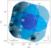 |
Fig. 1 Illustration of the first PLATO pointing field called LOPS2. The platform pointing (being parallel to the pointing of the two F- CAMs; see magenta star) is centred at the equatorial coordinate (α, δ) = (95.310 43°, −47.886 93°), with zero rotation with respect to the Galactic equator. The N-CAM overlap of nCAM ∈ {6,12,18,24} is illustrated with an increasing darker shade of blue (also indicated in the white boxes), and the blue, green, yellow, and red dot show the pointing of N-CAM group one, two, three, and four, respectively. The black transparent map highlights dense sky regions such as the location of the Milky Way plane, the Large Magellanic Cloud (LMC, encircled in orange), and a few globular clusters (pink circles, from Harris 1996). |
2 Overview of MOCKA
The MOCKA catalogue has been generated using the PLATO camera simulator, PlatoSim2 (Jannsen et al. 2024). Specifically, the PlatoSim software package provides a toolkit dubbed PLATOnium, which transforms PlatoSim (being a camera simulator) into a mission simulator, meaning that realistic instrumental systematics for the entire payload are easily configured in a coherent way in accordance to the number of co-pointing cameras and the mission requirements. With PlatoSim being an extremely feature-rich pixel-based simulator, PLATOnium greatly alleviates the manual process of setting up a new PlatoSim project, meanwhile being designed for parallel computing. Aside from instrumental systematics, the toolkit provides scripts to generate custom stellar sky catalogues (either using the PLATO input catalogues (PIC; Montalto et al. 2021) or the Gaia database (Gaia Collaboration 2016)), and realistic models of stellar variability (cf. Sect. 4).
Compared to the PIC, which focusses on FGKM dwarf and subgiant stars, the stellar catalogue used in this work is queried from the third data release (DR3; Gaia Collaboration 2023b) of the Gaia mission. Since the selection of the longduration observational phases (LOPs; Nascimbeni et al. 2022) a slight modification has been made to the LOP south (LOPS1 → LOPS2; Nascimbeni et al. 2025), which is the first definite pointing for PLATO. The choice of using the Gaia catalogue (as compared to a synthetic one) is based on: i) a more realistic distribution of relative pixel positions and brightnesses of target stars with respect to stellar contaminants and ii) a realistic crowding metric (e.g. more massive pulsators are found in crowded regions within the galactic thin disc; Bowman et al. 2022). In practice, the final LOPS2–Gaia DR3 catalogue was generated from full-frame CCD images of PlatoSim while injecting stars with 2 ≲ G ≲ 17 (cf. Appendix A).
Figure 1 shows the LOPS2 pointing in equatorial coordinates with the characteristic geometric feature of six co-pointing cameras, situated in four camera groups each with an opening angle of 9.2° relative to the platform pointing. The result is an overlap of the FOV for the so-called normal cameras (N-CAMs) counting nCAM ∈ {6,12,18,24}. Figure 2 shows the colour absolute magnitude diagram (CaMD) of stars from the LOPS2 within a distance of 1 kpc from the Sun. The ellipses represent the approximate regions of where each pulsating class is expected to be found.
Our catalogue contains three batches of simulated data for each stellar sample:
AFFOGATO is a best-case scenario where the instrumental systematics are ‘as expected’ and stellar variability from nearby contaminant stars is excluded;
CORTADO is a worst-case scenario regarding instrumental systematics but with ‘quiet’ stellar contaminants;
DOPPIO is a worst-case scenario regarding variable stellar contaminants (with all contaminants being variable) but with instrumental systematics ‘as expected’ by the mission.
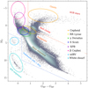 |
Fig. 2 CaMD of stars from the LOPS2 (see Fig. 1) within 1 kpc from the Sun. Here, G, GBP, and GRP refer to the Gaia full-bandwidth, blue, and red passband, respectively. Commonly known CaMD features are highlighted with coloured text. Each of the coloured circles indicates the approximate region of a stellar pulsation class that is a part of MOCKA. |
3 Stellar input catalogue
The LOPS2–Gaia DR3 catalogue shown in Fig. 1 contains 7,757,180 stars in the magnitude range 2 ≲ G ≲ 17 and forms the base from which we construct a target catalogue for each asteroseismic sample. Like any other survey, Gaia is magnitudelimited and suffers from several observational biases (e.g. Schönrich et al. 2019; Rybizki et al. 2022). To mitigate the inclusion of artefacts in our stellar samples, we start from the Gaia CaMD, shown in Fig. 2.
We first accounted for the extinction as measured in the Gaia passband, AG (GSP-PHOT). Our catalogue contains 6,602,912 stars with an extinction measurement. We consider these as our potential target stars (cf. Sect. 3.1). The remaining million or so (typically faint) stars without an extinction value may be a stellar contaminant. With an uncertain location in the CaMD, we assume that all of these stars have a zero extinction and we acknowledge the small bias this may entail in the target-to-contaminant magnitude distribution of our simulations (cf. Sect. 5.2).
Next, we converted the stellar magnitudes from the Gaia G passband to the PLATO N-CAM passband, 𝒫 (for a passband comparison, see Fig. 6 of Marchiori et al. 2019). The passband conversion is derived from atlases of stellar atmospheric models for dwarfs and giants (cf. Appendix B, using the Gaia colour, GBP − GRP). As shown in Fig. 2, we separated dwarfs from giants using an upper CaMD boundary (with giants above the dotted red line) as well as dwarfs from compact objects using a lower CaMD boundary (with compact objects below the blue dotted line). Determined from a linear fit to the red clump, the gradient of the boundary definitions is parallel to the direction of interstellar reddening, such that MG ∝ 1.6 (GBP − GRP).
3.1 Target star sky catalogue
Before we started to refine each asteroseismic sample, we first removed bright stars that will saturate the PLATO detectors. Jannsen et al. (2024) showed that for stars of 𝒫 ~ 7.5 mag, charge bleeding results in a non-conservative photometric measurement. Hence, we rejected 3175 bright stars with 𝒫 < 7.5 mag. To keep the analysis simple, we only sought to simulate targets as if they are all single stars. Following Penoyre et al. (2020), we excluded binaries by rejecting stars with a reduced unit weight error defined by Gaia in excess of 1.2. Moreover, we removed all stars without a measurement of either {G, GBP − GRB, AG, ϖ} and stars with extremely large relative parallax uncertainties (i.e. σϖ/ϖ > 1). After all these cuts, we were left with 5,683,986 potential target stars.
The base of each asteroseismic sample (except for compact pulsators) was constructed from a query of all stars defined by the ellipses of Fig. 2. Each ellipse was define based on known pulsators from Gaia Collaboration (2019, Fig. 3). Since these CaMD instability regions comply with approximately the mass range of intermediate to massive stars, the on-sky crowding metric per pulsation class is well conserved using this methodology. Next, each sample was trimmed using the respective gross spectral type ranges given in Table 1; except for γ Dor and δ Sct stars, for which further physical cuts are made (as we discuss in Sect. 3.2).
For each asteroseismic sample, we homogeneously assembled N★ stars, as indicated in the last column of Table 1. The choice of N★ was set by the number of potential targets available in each class after all cuts. We required that each sample have an equal observability count of nCAM ∈ {6, 12, 18, 24}, while having an approximately uniform star count over the range of apparent magnitudes 7.5 < 𝒫 < 17. The upper magnitude limit (𝒫max, Table 1) was adjusted given the detectability of the maximum amplitude for each type of pulsator. As an example, even though both are gravito-inertial pulsators along the main sequence, the γ Dor stars have lower amplitudes than the SPB stars (Van Reeth et al. 2015; Pedersen et al. 2021), implying that we simulated the former class only up to 𝒫 = 14 while the latter up to 𝒫 = 16. Each detection-magnitude threshold was set by PLATO’s noise budget derived from a separate set of simulations (cf. Appendix C). To conform to these requirements, we used a stellar magnitude histogram, corresponding to the four camera visibilities, as the inverse weight to randomly draw N★/4 stars in each nCAM-bin of each asteroseismic sample. We note that due to the effective number of a available targets in our limited Gaia catalogue, this methodology does not provide a perfectly equal (but still sufficient) count over each nCAM–𝒫 range (see Appendix D).
3.2 Target star parameters
We defined a stellar parameter space for each (target) star in order to apply an instrumental amplitude correction (cf. Sect. 4). This requires an estimate of the stellar mass, M, radius, R, luminosity, L, effective temperature, Teff, surface gravity, log 𝑔, and metal- licity, [Fe/H]. In the following we provide a short summary how the stellar parameter space of each asteroseismic sample was created, while leaving an in depth description to Appendix D for the interested reader.
At this stage, the majority of our target stars have { M, R, Teff, log 𝑔, [Fe/H]} defined by Gaia. Due to the strong model biases from the Gaia pipeline for these parameters regarding massive and evolved stars (and to some degree for lower mass dwarfs, e.g. Fritzewski et al. 2024a), we only rely the Gaia FLAME pipeline3 for the AF-type dwarfs, namely the γ Dor and δ Sct samples. While the selection of γ Dor stars was guided by the theoretical instability strip of Dupret et al. (2005, red lines of Fig. 3), the δ Sct stars were established using the observational instability strip of Murphy et al. (2019, orange lines of Fig. 3). The parameter space of the SPB and β Cep sample was artificially generated by defining a HRD polygon using evolutionary tracks and instability strips of Burssens et al. (2020, blue and purple lines of Fig. 3, respectively).
The parameter space of evolved stars was likewise artificially created. For the sample of RR Lyrae and Cepheid pulsators, each physical quantity was generated using a simple normal distribution while drawing the mean and standard deviations using literature results (see Tables D.1 and D.2, respectively). For the hot subdwarf B (sdB) and white dwarf (WD) pulsators, we also use literature values wherever possible (see reference of Sect. 4.1.7). Otherwise the parameter space was assigned using a best knowledge estimate given the spectroscopic and/or photometric information of each compact pulsator.
4 Models of variability
A huge number of stellar variables all across the CaMD have been discovered by ground-based surveys, such as OGLE (Udalski et al. 1992), and space-based missions, primarily by CoRoT, Kepler, K2, TESS, and Gaia. In particular, Gaia Collaboration (2019) cross matched several of the above surveys with the Gaia DR2 for the identification of variable sources.
To avoid introducing biases from sparse sampling and changing data quality from one survey to another, we generate each variable model using either a database of high-precision space-based photometric measurements or a theoretical framework.
Following the former option means finding a suitable sample for which pulsation modes (frequency, amplitude, and phase) can be used more broadly in a statistical sense. Then, starting from an equidistant time series, t (with a sampling of δt = 25 s, and a duration of Δt = 2 yr), we use a slightly modified formalism from Van Reeth et al. (2015) to create each light curve:
![$F(t) = A\left[ {{{f(t)} \over {\max [f(t)]}} - \left\langle {{{f(t)} \over {\max [f(t)]}}} \right\rangle } \right],$](/articles/aa/full_html/2025/02/aa52811-24/aa52811-24-eq1.png) (1)
(1)

Here, every ith pulsation mode has a cyclic frequency, ν (together with an angular frequency, ω = 2π v, and period, P = 2π/ω = 1/ν), along with the amplitude, a, and phase, ϕ. Also, A is the maximum peak-to-peak amplitude of the light curve, and the index, γ, describes the asymmetry of the pulsations in the time domain. We use γ = 2.2 for γ Dor and SPB stars (Van Reeth et al. 2015) and otherwise a power of unity4. Furthermore, throughout Sect. 4.1, a log-normal fit is used to describe the distribution of mode amplitudes, ai, from the stellar sample in question. In this work, we restrict ourselves to simulations based on stable frequencies, νi.
While this work uses observations from different instruments, a correction is needed to rescale the pulsation amplitudes observed in a given passband to that of the PLATO passband. This effect is particularly important for the current analysis of intermediate to massive stars, as the amplitude ratios of OBAF- type stars decrease with increasing central passband wavelength (e.g. Heynderickx et al. 1994; De Ridder et al. 2004; Hey & Aerts 2024; Fritzewski et al. 2024b). The passband correction (PC) is modelled5 as the quotient of the effective passband flux of a given star, which in turn is the product of the total spectral response, Sλ, and the spectral energy density, Fλ, from a synthetic spectrum:
 (3)
(3)
where SX is the response function for passband X (i.e. the PLATO passband) and Y is the response function for passband SY (i.e. the reference passband of the photometric data). When possible, we use the PHOENIX library (Husser et al. 2013) of high resolution spectral models as it covers a dense grid of stellar bulk parameters { M, R, Teff, log 𝑔, [Fe/H]}. Since the PHOENIX grid only extends to Teff = 12.2 kK, we use the ATLAS9 library (Castelli et al. 2003) for earlier spectral type stars (extending to Teff = 50kK).
Additionally, the finite data sampling of astronomical instruments also alters the observed amplitudes. This phenomenon is described by the amplitude visibility function (or ‘apodization’ cf. Hekker & Christensen-Dalsgaard 2017) which is a strong function of frequency (e.g. Bowman et al. 2016; Bowman & Kurtz 2018). Expressed in terms of the normalised sinc function, the apodization correction (AC) factor is given by:
 (4)
(4)
where a0 is the true signal amplitude and a1 is the observed signal amplitude. It is evident from Eq. (4) that the strongest suppression are near integer multiplets of the Nyquist frequency,  .
.
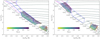 |
Fig. 3 HRD of the γ Dor and SPB (left panel), and δ Sct and β Cep (right panel) stellar samples. The colour gradient indicates the stellar surface gravity, and over-plotted are MIST evolutionary tracks (Choi et al. 2016). Solid lines indicate instability strips for gravity modes in the left panel and pressure modes in the right panel. The red lines show the edges of the theoretical γ Dor instability strip from Dupret et al. (2005) (corresponding to a mixing length of respectively αMLT = 2 (solid lines) and αMLT = 1.5 (dashed lines) in the left-hand plot). The orange lines represent the observational δ Sct instability strip from Murphy et al. (2019). The blue and purple lines are the theoretical instability regions of SPB and β Cep stars, respectively, calculated by Burssens et al. (2020). |
4.1 Target variables
To simulate the target variables, we primarily use Kepler observations, as this mission shares a similar photometric precision, a similar observing strategy, and instrumental systematics common for a spacecraft located in the second Lagrange point (L2), as planned for PLATO. Hereto, the 4-yr Kepler light curves serve as an excellent benchmark for creating the asteroseismic signals of our targets. For the remaining cases, light curves from TESS and OGLE were used due to their typical much larger sample size of variable stars.
4.1.1 γ Doradus stars
γ Dor stars are high-order non-radial g-mode pulsators whose oscillations are excited by the flux blocking mechanism at the base of their convective envelopes (Guzik et al. 2000; Dupret et al. 2005). They are intermediate mass (~1.2–2M⊙) Population I main sequence stars with oscillation periods between ∼0.2 and 3 day.
To generate the oscillation modes for each mock object, we use the sample of 611 Kepler γ Dor stars from Li et al. (2020) as benchmark. From this sample, three classes of oscillation modes dominate: dipole sectoral prograde g modes (l, m) = (1, 1), quadrupole sectoral prograde g modes (l, m) = (2, 2), and retrograde dipole Rossby (r) modes (k, m) = (−2, −1) with an occurrence rate of around 62, 19, and 12%, respectively. For simplicity, we generate synthetic light curves including only dipole sectoral g modes. Assuming that the period spacing changes linearly with period (imitating a smooth chemical gradient at the convective core boundary), we construct the mode periods, Pi, using the formalism by Li et al. (2020, typically used to construct a period-spacing échellogram):
 (5)
(5)
where P0 and ΔP0 are respectively the first period and first period-spacing in the pattern, Σ is the gradient of the periodspacing pattern, and ni = [(1 + Σ)1 − 1]/Σ is the normalised index, with ϵ = P0/ΔP0. A gradient in the period spacing pattern is a result of stellar rotation shifting the pulsation frequencies (Bouabid et al. 2013). Prograde modes, considered in this project, show a downward gradient as seen by an observer in an inertial frame of reference (Van Reeth et al. 2015; Aerts & Tkachenko 2024a).
Since the gradient and the mean period spacing are correlated (as a consequence of the stellar rotation rate), we model the gradient from a (arbitrary) best fit model to the dipole mode periods of lowest radial order:
 (6)
(6)
where {c1, c2, c3, c4, c5} are model coefficients. Figure 4 shows the model fit. From the Li et al. (2020) sample, we construct a kernel density estimation (KDE) for P0, ΔP0, and the total number of modes in the period-spacing pattern. A weighted extraction of these parameters was made, allowing for Σ to also be computed with Eq. (6).
While generating the mode periods with Eq. (5), care was taken to avoid unphysical period-spacing patterns that would imply a rotational velocity above the critical value (i.e. if vi > 3.3 d−1 the model generation was reset by drawing P0 again). Moreover, the peak of maximum amplitude may be either the first or last mode period, which is typically not observed (Van Reeth et al. 2015; Li et al. 2020). Hence the number index of this mode in the pattern is used to swap with the central mode period in the pattern. The number index is allowed for a random uniform offset of noffset ∈ [−5,5]. Lastly, using the model generation described above, a synthetic light curve for each star was iteratively generated using Eq. (1).
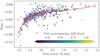 |
Fig. 4 Model fit to the gradient–period relation for dipole sectoral prograde g modes from Li et al. (2020). Typically this diagram features the mean period, but here we correlate the first mode period in the period spacing pattern with the gradient. The colour scaling shows the value of the corresponding first period spacing. |
4.1.2 Slowly pulsating B stars
Slowly pulsating B (SPB) stars are high-order non-radial g- mode pulsators, whose oscillations are excited by the opacity (κ) mechanism operating in the partial ionisation zone of irongroup elements (Dziembowski & Pamiatnykh 1993). These stars are intermediate-mass (∼2.5–8 M⊙) Population I main sequence, stars with oscillation periods between ∼0.2 and 3 day.
The Kepler sample of 26 SPB stars from Pedersen et al. (2021) was used to construct a model of the oscillation modes. Each noise-less light curve was computed following the same methodology as for γ Dor stars of Sect. 4.1.1, with the exception of Σ, which was drawn from its KDE distribution due to the low number statistics being disadvantageous for fitting it to a real Kepler sample. Figure 5 shows an example of a typical g-mode pulsation model of a SPB star.
4.1.3 δ Scuti stars
δ Sct stars are radial or low-order non-radial p-mode pulsators, whose oscillations are excited by the κ mechanism acting in the partial ionisation zone of He II (Aerts et al. 2010). Moreover, some δ Sct stars have moderate radial order p modes excited by turbulent pressure (Antoci et al. 2014, 2019). They are intermediate mass (∼1.5–2.5 M⊙) Population I stars with pulsation periods between ∼0.2 and 8 h. While these pulsators are found on the sub-giant branch, in this project, we only consider main sequence p-mode δ Sct stars.
We used the Kepler sample of 334 δ Sct stars from Bowman & Kurtz (2018) to generate a database of synthetic light curves. Amongst these multi-periodic pulsators, 187 stars were selected to confidently avoid residual instrumental systematics present in the short cadence data. Due to the highly complex oscillation patterns amongst δ Sct stars, we do not attempt to reproduce a physical model similar to that of the γ Dor and SPB stars. For this work, we simply draw the number of modes, frequencies, and amplitudes directly from the KDE distribution established from the Kepler sample.
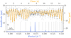 |
Fig. 5 Example of a simulated SPB star. The lower/left axes belong to the amplitude spectrum (blue line), where we have highlighted the mode frequencies (dotted lines), the first mode period (P0), and the first period spacing (ΔP0). The upper/right axes belong to the corresponding light curve (shown for the first 15 days) in its noise-less form (orange line) and simulated form (black points, representing a 𝓟 ≈ 10.3 star observed with nCAM = 6). |
4.1.4 β Cephei stars
β Cep are low-radial order p- or ɡ-mode pulsators whose oscillations are excited by the κ mechanism acting in the partial ionisation zone of iron elements (Dziembowski & Pamiatnykh 1993; Gautschy & Saio 1993). The β Cep stars are high mass (~8–25M⊙) Population-I stars, and their oscillation periods range between a few hours to several days. Most of them are main sequence stars, but a significant fraction are (sub-)giants (see Burssens et al. 2020).
As benchmark for the generation of oscillation modes, we use a sample of 196 β Cep stars initially assembled by Gaia Collaboration (2023a) using Gaia DR3 observations and further refined and validated by Hey & Aerts (2024) and Fritzewski et al. (2024b) using TESS observations. Among this sample, 93 objects were already catalogued by Stankov & Handler (2005). The model generation of β Cep mock stars follows that of the δ Sct sample (see Sect. 4.1.3).
4.1.5 RR Lyrae stars
RR Lyrae stars are often called ‘classical radial pulsators’ whose p modes are driven by the κ mechanism acting in the partial ionisation zone of He I (Stellingwerf 1984). They are metal-poor, low-mass (~0.5–0.9 M⊙) Population-II horizontal branch (i.e. He-shell burning) stars, where the majority pulsate in a dominant radial mode with period from ~0.2–1 day. Originally from Bailey’s classification scheme, today RR Lyrae are classified into RRab, RRc, and RRd types based on the amplitude and skewness in the light curves (e.g. McNamara & Barnes 2014; Bono et al. 2020). A significant fraction of the RRab and RRc stars shows long-term amplitude and phase modulations, also known as the Tseraskaya-Blazko effect (Blazko 1907).
While partly being based on the work of Molnár et al. (2022), we use a sample of 1538 synthetic RR Lyrae templates derived from TESS observations. Among these, we have 1105 RRab (99 being Tseraskaya-Blazko) stars, 382 RRc (17 being Tseraskaya-Blazko) stars, and 56 RRd stars. With such an abundant database of variable models we generate each noiseless light curve by simply drawing a source with replacement from the sample and introduce a small perturbation to the mode frequencies and amplitudes. We allow for a constant (multiplicative) shift of all amplitudes of ±10% compared to the dominant mode amplitude (resulting in a variety of light curve shapes seen for real RR Lyrae stars). Next, the first mode frequency was perturbed by ±10% and the subsequent frequencies were adjusted proportionally, based on the original frequency ratios.
4.1.6 Cepheid stars
Cepheid variables also belong to the class of ‘classical radial pulsators’ excited by the κ mechanism. While evolved stars of different masses may cross the classical instability strip at various evolutionary stages, the classification of Cepheids is quite diverse, forming three groups: classical Cepheids, anomalous Cepheids, and type II Cepheids (see Aerts et al. 2010, for a review).
While partly being based on the work of Plachy et al. (2021), we use a database of 2703 variable templates derived from TESS observations. Amongst 1339 classical Cepheids, our database contains 902 fundamental-mode, 366 overtone, and 71 double-mode pulsators. Amongst 264 anomalous Cepheids, our database contains 170 fundamental-mode and 94 firstovertone pulsators. Amongst 1078 type II Cepheids, our database contains 512 BL Herculis, 503 W Virginis star, and 63 RV Tauri stars. We follow the same methodology as used for the RR Lyrae sample to generate each mock object (see Sect. 4.1.5).
4.1.7 Compact pulsating stars
sdB stars are evolved low- to intermediate-mass stars that have survived core helium (flash) ignition, and now populate the extreme blue end of the horizontal branch (Heber 2009, 2016, see Fig. 2). Pulsating sdB (sdBV) stars come in two flavours: V361 Hya and V1093 Her variables, both with modes excited by the κ mechanism acting in the partial ionisation zone of iron elements (Charpinet et al. 1997; Fontaine et al. 2012). V361 Hya stars are slightly hot sdB stars with short-period (~1–13 min), non-radial, low-order p modes. V1093 Her stars are on the other hand slightly cooler pulsating sdB stars with long-period (~1–3 h), non-radial, low-order g modes. From the catalogue of 256 pulsating sdBV stars compiled by Uzundag et al. (2024), we use the 17 richest pulsators observed by Kepler suited for asteroseismic analysis. Among these, two are V361 Hya stars and 15 are V1093 Her stars.
Being the end product of stellar evolution for most (low- to intermediate mass) stars, WDs may enter one of three main instability regions as they slowly cool (i.e. DOV, DBV, and DAV). Which instability region they (potentially) enter depends on their atmospheric composition (see the reviews of Fontaine & Brassard 2008; Winget & Kepler 2008; Córsico et al. 2019). While Kepler/K2 provided high-precision photometry for 27 DAV stars (e.g. Hermes et al. 2017a, Table 1), only three DBV stars (Østensen et al. 2011; Duan et al. 2021; Zhang et al. 2024) and one DOV star (Hermes et al. 2017b) were observed. In contrast, the on-going TESS survey has so far provided an abundant catalogue of WD pulsators, especially for H-deficient WDs. Considering the photometric precision and sample coverage, we simulate in total 30 WD pulsators with the highest number of detected modes, which includes 10 DAV Kepler/K2 stars (Mukadam et al. 2004; Voss et al. 2006; Gianninas et al. 2006; Greiss et al. 2014, 2016), 10 DAV TESS stars (cf. Bognár et al. 2020; Romero et al. 2022; Uzundag et al. 2023; Romero et al. 2023), 5 DBV TESS stars (cf. Bell et al. 2019; Córsico et al. 2022b; Córsico et al. 2022a), and 5 DOV TESS stars (cf. Córsico et al. 2021; Uzundag et al. 2021, 2022; Oliveira da Rosa et al. 2022; Calcaferro et al. 2024).
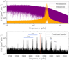 |
Fig. 6 Power spectral density (PSD) diagrams showing granulation and pulsation signals caused by large convective envelopes in low-mass dwarfs. The PSD was computed for a 2-yr noise-less light curve. The bottom panel is a zoom-in on the combined model illustrating the standard envelope of excited modes (used to estimate the frequency of maximum power, νmax) and the small (δv) and large (Δv) frequency separations. |
4.2 Contaminating variables
With FGKM-type dwarf stars being the key residents among our stellar (contaminant) catalogue, we additionally need to model their variability. Solar-like (FGK dwarfs) stars can exhibit convection-driven stochastic oscillations and various phenome- nas of stellar activity (e.g. granulation and star spots), whereas M dwarfs are known to be magnetically active leading to frequent events of energetic flares. In the following we describe our adapted model for variable contaminants, including eclipsing binaries and a group of miscellaneous variables.
4.2.1 Solar-like oscillations
To generate convection-driven variability of solar-like stars in PLATO passband, we follow Jannsen et al. (2024). In essence the stochastic oscillations are generated using 96 distinct pulsation mode frequencies of the Sun from the observational network BiSON (Chaplin et al. 1996; Davies et al. 2014; Hale et al. 2016) and using asteroseismic scaling relations from Kjeldsen & Bedding (1995). Granulation is modelled with two super- Lorentzian functions (cf. Kallinger et al. 2014) while scaling amplitudes using the methodology of Corsaro et al. (2013). The oscillation and granulation signals are modelled in the time domain directly using the formalism of De Ridder et al. (2006). Lastly, we use high resolution PHOENIX spectra to calculate the bolometric correction and scale the amplitude spectrum to what is expected in the PLATO passband. Figure 6 shows a model example of a solar-type star.
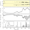 |
Fig. 7 Illustration of a stellar on-axis activity model for a solar-like star simulated for two years. (a) Spot emergence diagram with the black dots being their latitudinal location and relative sizes at emergence with respect to the stellar surface. (b) Stellar surface area covered by spots (in percentage). (c) Relative flux darkening by the spot coverage (in ppt) as function time. (d) Relative flux brightening by stellar flares (in ppt) as function of time. |
4.2.2 Star spots
Stellar activity of solar-type stars is an important and non- negligible photometric noise component for PLATO photometry. From an observational point of view, stellar activity generally imprints itself as cyclic rotational modulations due to the presence of dark optical spots and bright faculae (and networks of the latter, so-called prominences), and transient events such as flares. In the effort of modelling spot modulations of solar-type stars in a broader scope for the PLATO core science program, we developed the code pyspot. We describe the functionality of the software in Appendix E. In short, most parameter are being derived or selected at random from distributions based on Meunier et al. (2019, and references therein). Figure 7 shows an example of the code’s output, with panel a, b, and c showing the spot emergence diagram, the spot coverage diagram, and the relative flux diagram as function of time, respectively.
4.2.3 Stellar flares
Flares are high energetic phenomena caused by reconnection of magnetic fields in the stellar atmosphere (Sun et al. 2015). Their dramatic increase of brightness, lasting on the order of minutes to hours, challenge the post-processing of space-based photometry, hence making them important to include in our simulations. To be representative of real stellar flares, we use the analytic model of Davenport et al. (2014) which is based on a sample of more than 6100 single flare events of the M dwarf star GJ1243 that was observed by Kepler. This model describes a fast polynomial rise and a two-phased exponential decay (cf. Eq. (1)–(3)). Tovar Mendoza et al. (2022) improved the model of Davenport et al. (2014) using a more robust subsample of flares from GJ1243 and modern statistical methods. This model is not yet implemented in PlatoSim. With only slight differences between the two flare templates, the improved model is expected to have a minimal impact on the asteroseismic yields of this project, but a greater impact is expected for extrinsic variability research (such as eclipse signatures).
Given the difference in internal structure and magnetic topology of FGKM dwarf stars, we use the spectral type dependent distributions of Van Doorsselaere et al. (2017) to draw the amplitudes (Fig. 4) and the occurrence rates (Fig. 6) for each star. Using the occurrence rate, the total number of injected flares was scaled by the activity rate (compared to solar) determined by the software pyspot. Each flare duration is drawn from a uniform distribution between 1 and 200 min, and following scaled to the flare amplitude such that more energetic events last longer. Finally, the spot coverage (also provided by pyspot) is used as weight while drawing the times of peak flaring flux. Hence, the flare occurrences realistically follow the stellar magnetic cycle, as illustrated in Fig. 7d for an active solar-like star.
4.2.4 Eclipsing binaries
The multiplicity fraction is a rapidly increasing function with mass, meaning almost all OB-type stars are found in multiple star systems (see Offner et al. 2022, for an overview). Especially, eclipsing binary (EB) systems are overly presented in all-sky surveys (IJspeert et al. 2024). For simplicity, we only model EBs (ignoring higher orders of binarity, cataclysmic binaries, attached systems, etc.) with an intermediate to massive star primary. Moreover, exoplanet transits are excluded in this project as they would have a minimal effect on our analysis.
We used a database of 3155 EB candidates observed by TESS from IJspeert et al. (2021), out of which 2946 systems were confidently selected as genuine EB systems. This catalogue contains detached main sequence EBs with an OBA-type dwarf primary.
4.2.5 Miscellaneous variables
All other stellar objects, not catagorised photometrically in previous subsections (acknowledging our enforced pigeonholing)6, are placed into a class of miscellaneous variables. We divide this class into long-period variables (LPVs) and short-period variables (SPVs). Generally, LPVs are red giant stars that populate the reddest and brightest regions of the CaMD and consist in terms of oscillatory behavior of Mira stars, semi-regular variables, slow irregular variables, and small-amplitude red giants. Due to the custom detrending approach employed in this work (which removes any trend longer than ~30 d; see Sect. 5.4), LPVs are not considered as target stars but only as stellar contaminants. We use the extensive library of LPVs from OGLE (Udalski et al. 2008, 2015) for the model generation.
Being part of PLATO’s calibration strategy, short-period chemically peculiar ApBp stars show extremely stable photometric signatures of chemcial spots that cause rotational modulation. From current studies we expect around 10% of all B5-A5 stars to possess a fossil magnetic field and therefore exhibit stable rotational modulations caused by chemical stratification (i.e. spots) in such stars (Renson & Manfroid 2009; Chojnowski et al. 2019; Mathys et al. 2020). Hence, a significant fraction of these stars are expected in the PLATO FOV. We simulate their noise-less light curves by drawing the rotational frequencies from a uniform distribution covering the usual [1, 3] d−1. The light curve shapes of these stars is modelled with a simple sinusoid with occasional contribution of the second harmonic. While the amplitude modulations of these stars observed by Kepler (Holdsworth 2021) and TESS (Holdsworth et al. 2021, 2024) are typically below 3G mmag, we assume that all are high amplitude BpAp stars with an amplitude distribution of 10–30 mmag in the PLATO passband.
5 Simulations
5.1 Spacecraft systematics
Instrumental systematics are crucial to include in any realistic set of simulations (e.g. Börner et al. 2024). PlatoSim provides a wealth of options and features to configure the PLATO payload in this regard (Jannsen et al. 2024). In this project we configure PlatoSim with settings from the PLATO mission parameter database (MPDB)7. Common for all simulations we assume that the properties of each camera (i.e. the telescope optical unit and the optics; Munari et al. 2022; the detectors and the front-end electronics; Koncz et al. 2022) are identical and that their noise sources are uncorrelated. All simulations include cosmic rays with a constant hit rate of 10 events cm−2 s−1. Moreover, an analytic model of the point spread function (PSF; mimicking the expected variation in PSF morphology across the focal plane) was used and charge diffusion was activated using a Gaussian kernel of 0.2 pixel.
From a computational point of view, the most important systematics to consider are pointing error sources that may impact the shape and stability of the PSF, meanwhile introducing a pixel displacement of the PSF barycenter in the CCD focal plane. In particular, two systematic errors that alter the location of the PSF on the CCD are camera misalignments (see Royer et al. 2022) and imperfect pointing repeatability between consecutive mission quarters. We account for these by randomly drawing the camera pointing and the platform pointing from a uniform distribution with a 3σ confidence that the error is below that of the mission requirements. Furthermore, we apply differential kinematic aberration (DKA) using a realistic L2 orbit.
We differentiate the configuration of random and systematic noise sources between the three simulation batches: AFFOGATO, CORTADO, and DOPPIO. Drawing all parameters from the PLATO mission database, AFFOGATO and DOPPIO complies to the MPDB ‘as expected’ instrument design, whereas CORTADO comply to the MPDB ‘as required’ instrument design. In particular, the only difference between AFFOGATO/DOPPIO and CORTADO regarding spacecraft systematics are the differences in settings for detector noise, the attitude and orbit control system (AOCS) jitter, and the thermo-elastic distortion (TED) of the payload. Table 2 shows the noise parameters related to the PLATO detectors given their requirement; a linear fit between beginning-of-life (BOL) and end-of-life (EOL) values is used to properly account for the time dependence of the CCD/FEE read noise and the dark current, which is updated at the beginning of each mission quarter.
A common AOCS red noise jitter model sampled at 0.1 Hz was used, but the root mean square (rms) values of the Euler angles {yaw, pitch, roll} are configured differently: AFFOGATO and DOPPIO use {0.036, 0.034, 0.040} arcsec, and CORTADO uses {0.144, 0.136, 0.160} arcsec. The former values correspond to the rms values extracted from the simulations of a dynamical AOCS model representative for the mission requirements ‘as expected’. The TED for each camera and mission quarter is included using a second order polynomial model whilst uniformly drawing the model coefficients under the restriction that the amplitude in yaw, pitch, and roll cannot exceed 9 arcsec and 2.25 arcsec (being equivalent to 0.6 pixel and 0.15 pixel)8 in three months, respectively. We further use a dynamical TED model to realistically add the repeating pattern of momentum dumps of the reaction wheels with a typical amplitude of ~30 ppm (which will happen every three days for PLATO). Next, a TED time series is created for each camera group via small perturbations in order to simulate a more realistic distribution of correlated noise across the platform. In summary, the AOCS jitter and TED amplitudes for CORTADO are four times larger than those of AFFOGATO and DOPPIO.
Configuration parameters for the PLATO detectors.
5.2 The pixel subfield
For each simulation (i.e. star+camera+quarter configuration), only contaminant stars within a radial distance of 45 arcsec (equivalent to three pixels in the CCD focal plane) away from their corresponding target star are simulated. Although our stellar catalogue is complete up to 𝓟 ~ 17, to avoid a negligible contribution from faint stellar contaminants for the brighter targets, a relative target-to-contaminant magnitude threshold of Δ𝓟 = 5 was used (being equivalent to an intensity ratio of 100) to limit the number of contaminants in a single subfield.
As part of keeping the PLATO telemetry budget at a minimum, small 6 × 6 pixel imagettes, will be placed around each (non-saturated) target star. The usage of the imagettes in this project is however undesirable since long-term drifts of a star’s barycentric position may move it outside the subfield and thus cause flux anomalies. By design, the subfield is always placed around a target star such that the target is within the central pixel of the subfield (i.e. maximally half a pixel offset from the central intra-pixel position). From the inclusion threshold of stellar contaminants, this means that all contaminants, before considering barycentric drift, are located within a central circular aperture of 6.5 pixel in diameter. In principle the maximum amplitude for the DKA can be as high as 0.8 pixel per mission quarter (Samadi et al. 2019). However, for the vast majority of cases the DKA amplitude is much lower. Hence, the combined (TED and DKA) pixel displacement in a single mission quarter rarely exceeds 1 pixel. Thus, even for a worst case scenario of having the longterm drift purely in a horizontal or vertical direction, a 8 × 8 pixel subfield is an optimal trade-off regarding computational speed and preventing flux anomalies.
 |
Fig. 8 Gaussian KDE distribution per spectral type of the LOPS2–Gaia DR3 single stars with valid stellar bulk parameters. The normalised density is scaled from low to high with brown to purple colour, respectively. A cut in the density region, discarding the lowest 25–50%, has been made to each spectral type to better confine each region. |
5.3 Variability injection for contaminants
For PlatoSim the variable injection happens at pixel-level and at run time. Thus, the database of noise-less light curves (cf. Sect. 3) were considered. For AFFOGATO and CORTADO, only the target star is variable and the injection follows the procedure described in Sect. 4. For DOPPIO, we also injected stellar variability into the contaminants, for which we first check for binaries (cf. Sect. 3.1). If a contaminant star belongs to one of the 853 869 sources in our catalogue classified as a binary system, we then randomly draw an EB model from our database (cf. Sect. 4.2.4). If it is not a binary system, the classification continues to the next stage for single stars.
In the single star stage, we first checked that the stellar parameters { M, R, Teff, log ɡ, [Fe/H]} have been defined for all stars within the sub-field. Since Gaia does not always provide these bulk parameters, we draw them from empirically estimated KDE distributions as in Fig. 8, assembled into spectral types provided by Gaia. Each spectral type KDE is created from the subset of stars with valid stellar parameters, meanwhile an arbitrary 25– 50% density cut is used to remove potentially spurious solutions. It is clear from the unphysical bimodal structures (i.e. for O, A, and M-type), that the Gaia pipeline suffers from systematic biases. The spectral type tag CSTAR are candidate carbon stars (whose complex morphology we ignore in this project) and the unknown spectral types are typically non-stellar or extragalactic objects. Furthermore, a smaller group of stars do not have any spectral classification (in total 27 981 objects; i.e 0.4% of our catalogue), hence we merged these into the group of unknown stars. For each star, we retrieved the stellar parameters using three cases based on Fig. 8: (i) If the effective temperature and the colour are known, we select a star (and its parameters) from a closest match to these parameters of the respective KDE distribution; (ii) if a star only has colour information, this is used to draw a star along a horizontal slice of the KDE for a given spectral type; (iii) if no colour information is available and only the spectral type of a star is known, a direct weighted draw from the KDE distribution is performed.
With each contaminant having a complete set of stellar parameters, we first check if a contaminant belongs to any of the pulsation classes of MOCKA. If true, we create its model as explained in the respective subsection of Sect. 4.1. If false, we consider variability of lower mass dwarf and giant stars. As outlined in Sect. 4.2, depending on the stellar parameters and magnitude cuts, we model stars later than spectral type F5 using one or more of the components: granulation, stochastic oscillations, spots, and flares. We introduce cuts in the CaMD using a linear relation of the form: MG = a (GBP − GRP) + b, with model coefficients {a, b).
Since dwarf, subgiant, and giant stars of spectral type F5-K7 have a convective envelope, the expectation is that all of them are solar-like oscillators. We first confine red giant stars in the CaMD within an upper boundary using (a, b) = (1.6, −3.6) and a lower boundary using (a, b) = (1.6, −0.6), respectively. Further we require that GBP − GRP > 0.5 and log ɡ < 3.8 (Fig. 9a). We confine solar-type (main sequence and sub-giant) stars using the lower red giant star boundary in addition to a CaMD cut using (a, b) = (−10, 8), while further requiring that log ɡ > 4.2 (Fig. 9b). We furthermore confine rotational spotted variables in CaMD using the observational dearth of these stars below GBP − GRP < 0.4 (e.g. see Gaia Collaboration 2019), which theoretically corresponds to the transition region between stars having radiative versus convective outer envelopes (Kippenhahn et al. 2013). To increase the variety among the solar-like stars, each star is assigned a stellar flare probability based on its spectral type being p(F, G, K, M) = (20%, 80%, 90%, 100%). Lastly, we confine active M dwarfs using the cuts of GBP − GRP > 1.7 and MG > 6. Shown in Fig. 9c, these red dwarf stars were modelled to have spots and flares.
If it is not assigned as a binary (see Fig. 9d), a solar-like oscillator, or a red dwarf, the classification simply assumes that the stellar contaminant is a miscellaneous variable. As mentioned in Sect. 4.2.5, we model short and long period miscellaneous variables. Shown in Fig. 9e, we confine LPVs in the CaMD as those above the upper red giant boundary and with GBP − GRP > 0.8. Lastly, any star with an unknown spectral classification (see Fig. 9f) is simply classified as a SPV. Hence, we artificially increase the noise budget by assuming that all extra-galactic objects are SPVs.
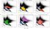 |
Fig. 9 CaMD of different stellar classes used to assign a variable signal to stellar contaminants. The respective class is written in the title header together with the number count of the class. The upper panels show the confinement of all stars that feature solar-like variability: (a) red giants, (b) solar-like dwarfs and subgiants, and (c) red dwarfs. The lower panels show the confinement of (d) binaries, (e) giants and compact objects (above the purple line and below the blue lines, respectively), and (f) all objects with an unknown spectral type. The black points are all stars in the LOPS2 (G ≲ 17), whereas the metallic contour defines stars within 1 kpc from the Sun. |
5.4 Photometric pipeline
The GO programmes of PLATO, demanding on-board photometry, will rely on an optimal aperture mask algorithm by Marchiori et al. (2019). This algorithm is implemented in PlatoSim and constructs a pixel mask based on a simple trade-off between lowering the noise-to-signal ratio (NSR) while mitigating stellar contamination. In particular, the algorithm defines a stellar pollution ratio (SPR; an important parameter for the forthcoming analysis) measuring how much contaminating flux leaks into the aperture mask. As part of the mission strategy (Rauer et al. 2024), the aperture mask of each star may be updated periodically during a mission quarter given that a lower NSR can be achieved. The mask-update frequency is currently undecided. Hence, to be conservative, we choose an update every 30.5 d (which may or may not enforce a trigger twice per quarter).
As illustrated by Jannsen et al. (2024, Fig. 18), the current best estimate of a single PLATO camera light curve shows several levels of instrumental systematics. The three dominant instrumental features are the long-term trends caused by displacement of the PSF barycenter (due to the effect of TED, KDA, etc.), large jumps in the mean flux level between consecutive mission quarters (due to changes of optical throughput), and a slow continuous flux decrease (due to ageing effects). Additionally, relevant for the on-board photometry, mask-updates likewise introduce jumps in the mean flux level.
While the official post-processing pipeline is still under construction, we have implemented a simple reduction pipeline needed to perform our analysis. Several sub-modules of the official post-processing pipeline exist (e.g. the REPUBLIC detrending algorithm; Barragán et al. 2024). Hence, as a better performance is expected from the official pipeline, the employed pipeline should be a conservative approach with respect to the removal of systematics (potentially counteracting the increased complexity of reality versus simulations). Appendix F shows each of the reduction steps presented in the following.
To correct for the long-term systematic trends in the light curves, we use a polynomial model for detrending the signal of each individual camera and mission quarter segment. If a mask-update was triggered, each sub-segment was detrended individually. To account for the varying segment lengths (i.e. roughly 30, 60, and 90 d) we perform a model comparison between a polynomial fit of first to fourth degree by obtaining the Bayesian information criterion (BIC) probability:
 (7)
(7)
where ΔBIC ≡ BIC − BICmin and BIC being determined from each ordinary least squares fit. The model with the highest BIC probability was selected for the fit.
Outliers were removed only after the detrending to avoid sharp features in the light curve (e.g. flux jumps due to mask- updates) to be flagged as outliers. Closely resembling PLATO’s on-board outlier rejection algorithm, we employ the software Wōtan9 (Hippke et al. 2019) and use an upper and lower threshold in multiples of the median absolute deviation (MAD) with the following magnitude dependence:
 (8)
(8)
From empirical tests, the length of the filter window was set to half a day, and the middle point in each window was calculated using the median.
For each star, the multi-camera and multi-quarter light curves were combined to a single dataset. Next, a second iteration of the outlier removal was applied following the procedure described above. Data points sharing the exact same timings (i.e. camera observations from the same camera group) were averaged. Depending on the pulsation class, the final light curve per star was sampled at a cadence of δt = {25, 50, 600) s (cf. Table 1), corresponding to a Nyquist frequency of  , respectively10.
The uncertainty on the flux measurements was computed as the internal scatter in the time series to account for all additional sources of error introduced by previous reduction steps. From a computational point of view, σ was calculated using a carbox filter of size N. Hence, for each time stamp i, we equated the fractional uncertainty by calculating a short-term filter σi(N = 1 h). To robustly estimate the uncertainties in the presence of intrinsic stellar variability, a long-term filter µi(N = 10 d) was applied to the filtered signal and used as the mean flux error.
The final light curves of MOCKA span two years and include quarterly data gaps of exactly one day (allowing for a custom mission downtime distribution to be applied). As shown in Fig. 10, a realistic distribution of data gaps was introduced for further analysis in this project. This was done to properly account for the impact on the asteroseismic analysis from a degraded window function (e.g. García et al. 2014; Pascual-Granado et al. 2018).
In line with the latest performance study, we apply interquarter data gaps (approximately every 91 d) with a duration of ΔTi = 1.5 + 𝓤(−0.5,0.5) d, where a duration anomaly (drawn from a uniform distribution) was included. To maintain PLATO’s nominal Lissajous orbit around L2, a station-keeping manoeuvre is planned every 30d. As the duration of these manoeuvres is still unknown, we conservatively estimate it to be ΔTi = 2.5 + 𝓤(−0.5, 0.5) h. Lastly, using statistics from the 4-year Kepler mission, we further introduced data gaps from coarse pointing events (i.e. temporary loss of fine guidance resulting in an increased photometric scatter) and safe mode events (i.e. temporarily operation shut-offs due to unexpected events). The duration of these two events was computed with ΔTi = 30 + 𝓤(−15, 15) min and ΔTi = 1 + 𝓤(−0.5, 0.5) d, respectively11.
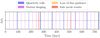 |
Fig. 10 Assembly of data gaps included prior to the frequency analysis. Besides the quarterly rotational realignment of the spacecraft (blue lines), we also consider downtime due to station keeping manoeuvres (purple lines), loss of fine guidance (orange lines), and safe mode events (red lines). |
5.5 Frequency extraction
With the delivery of high-quality space-based data, the recovery of mode frequencies increasingly depends on the iterative prewhitening strategy employed (e.g. see Van Beeck et al. 2021, for a comparison between five different methods for g modes in SPB stars). The frequency extraction in this work was performed with the software STAR SHADOW12 (IJspeert et al. 2024). Although developed for the detection of eclipsing binaries, this software contains a robust iterative prewhitening procedure: i) it extracts the frequency of the highest amplitude one by one, directly from the Lomb-Scargle periodogram (Lomb 1976; Scargle 1982) as long as it reduces the BIC of the model by ∆BIC < 2, and; ii) a multi-sinusoid non-linear least-squares optimisation is performed, using groups of frequencies to limit the number of free parameters.
We emphasise that the prewhitening strategy used by STAR SHADOW is conceptually different from a more standardised procedure of invoking a stopping criterion based on the signal- to-noise ratio (S/N). Thus, as an alternative to the ∆BIC < 2 stopping criterion, we extended the iterative prewhitening module of STAR SHADOW, implementing a S/N stopping criterion. In our analysis, we recorded all extracted frequencies until a certain S/N threshold. A commonly used criterion is S/N = 4, which has been empirically determined from ground-based observations of p-mode oscillators by Breger et al. (1993). The validity of this criterion in comparison to space-based surveys is however questionable (e.g. see Baran et al. 2015; Zong et al. 2016; Baran & Koen 2021; Bowman & Michielsen 2021). In fact, the premise of a standardised S/N criterion relies on the assumption of Gaussian noise, in which only the cadence, δt, and number of data points, N, are model parameters (Baran & Koen 2021).
We investigated what S/N criterion is optimal for PLATO light curves as function of sampling δt ∈ {25, 50, 600} s and number of mission quarters nQ ∈ [1, 8]. We assume that two days are lost due to downtime (approximately agreeing with Fig. 10), meaning that a mission quarter of ∼89.31 d contains N = {304128, 152064, 4224} data points for the nominal, twice nominal, and long N-CAM cadence, respectively. We generated 10 000 synthetic light curves, including only white noise for each duration and sampling, and used, for consistency, STAR SHADOW to compute the Lomb-Scargle periodogram of each light curve up to the Nyquist frequency. Following Baran & Koen (2021), the amplitude spectrum was standardised using its median to get rid of the dependence of the rms average noise level. The S/N value of the highest amplitude peak was computed as the ratio between the peak-amplitude and the local noise level using a 1 d−1 frequency window in the residual periodogram. Lastly, we calculate the false alarm probability (FAP) from the resultant histogram. Figure 11 shows an example of the computed criterion for nQ = 8 and FAP = 1%.
Baran & Koen (2021) showed that the S/N(nQ) can be described by a simple logarithmic relation. This is also true for S/N(FAP) due to the log-normal behaviour of the S/N histograms (see Fig. 11). Performing the above exercise for each cadence, mission quarter duration, and over a semi-regular grid of FAP ∈ [0.01, 10]%, results in a so-called significance criterion surface for each cadence:
 (9)
(9)
where the best fit coefficients {d1, d2, d3} are listed in Table 3. Eq. (9) states that the S/N criterion is increasing: (i) the shorter the cadence; (ii) the longer the duration of the time series, and; (iii) the lower the FAP. The latter two interferences are clearly illustrated in Fig. 12 showing the best-fit S/N surface to the simulations with a 25 s cadence.
It is worth noticing that for the most commonly adopted thresholds in the literature of FAP = 1% and FAP = 0.1%, the optimal S/N is always larger than four, independent of the duration of the light curve. This highlights that the traditional threshold is too optimistic for continuous space-based data (agreeing with previous studies, e.g. Degroote et al. 2010; Baran et al. 2015). Furthermore, since PLATO light curves consist of co-added observations of multiple cameras, residual instrumental systematics are difficult to avoid. Instrumental systematics typically show excess power at low frequencies in amplitude spectra, which increases the probability of detecting higher amplitude noise peaks. Thus, any S/N value determined using Eq. (9) should be seen as a lower boundary when dealing with long-period variable signals. In the forthcoming analysis, the S/N threshold computed for nQ = 8 and FAP = 0.1% were selected, which for δt ∈ {25, 50, 600} s are S/N ∈ {5.76, 5.63, 5.34}.
As part of the final post-processing step, we computed the frequency and amplitude precision of the pulsation modes from the amplitude spectrum (see Fig. F.5 for the workflow), rather than from analytical formulae as in Montgomery & O’Donoghue (1999) or an adaptation of it as in Zong et al. (2021). STAR SHADOW uses more advanced numerical techniques to compute the frequency and amplitude precisions (see IJspeert et al. 2024, for details). From the list of observed pulsation modes (extracted using the BIC criterion), we queried and matched each mode one by one to the list of injected modes. First, this was done by searching for all possible modes within a 0.1 d−1 frequency window from the injected mode frequency. If multiple mode frequency candidates were found, a closest match to the input frequency and amplitude was computed by minimising  , with
  and
and  being the relative difference between the observed and injected amplitude and frequency, respectively. Next, a residual diagram in frequency and amplitude was computed based on the matched modes. Finally, a root mean square (rms) estimate of the frequency and amplitude precision were calculated for pulsation modes detected with both the BIC and S/N criterion. This procedure was repeated for each star, while the (noise) peak of smallest amplitude was additionally recorded. We note that rms frequency precision in this project is a simple approximation, since the ‘real’ frequency precision depends on many factors (e.g. see Bowman & Michielsen 2021). In the next section we present the results of the combined frequency extraction for the γ Dor and SPB star samples.
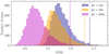 |
Fig. 11 Histogram of the S/N of the highest amplitude frequency extracted from 10 000 synthetic white noise PLATO light curves. This example shows the optimal S/N criterion (dashed lines) estimated as the FAP = 1% from time series with a duration of eight mission quarters. |
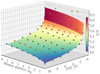 |
Fig. 12 Optimum significance surface for PLATO light curves with a cadence of δt = 25 s. The surface fit was performed with Eq. (9) to the grid points (sorted in colour after the FAP, with semi-regular grid points of {10, 8,6,4,2, 1, 0.5, 0.1, 0.01}%). |
6 Results: g-mode pulsators
6.1 Noise budget in the frequency domain
We start by considering the limiting amplitude that can be retrieved from prewhitening in the presence of random and systematic noise. Figure 13 shows the result as computed from each stellar light curve of the AFFOGATO (high amplitude, cf. Sect. 6.2) SPB sample as a function of magnitude and camera visibility. As expected from the NSR estimates in the time domain, the amplitude detection limit is a clear function of the camera visibility, with the smallest amplitudes being retrieved from light curves combined from 24 N-CAMs.
Compared to the NSR estimate in the time domain, the amplitude detection limit is an order of magnitude lower when applying modern prewhitening strategies like that of STAR SHADOW. We highlight that the simulation batch AFFOGATO is mainly dominated by Gaussian-like noise, i.e. the underlying noise model is well described by a jitter, photon, and sky/detector dominated noise regime (cf. Fig. C.1; see also Börner et al. 2024). With PLATO covering variable signals with amplitudes ranging from ppm to ppt level, Fig. 13 shows that for the expected operation of 24 N-CAMs, PLATO will be able to detect peaks in the periodogram below 10 ppm, 100 ppm, and 1000 ppm for 𝒫 ≲ 12, 𝒫 ≲ 15, and 𝒫 ≲ 17, respectively.
Although we have illustrated that the underlying amplitude distribution for most pulsating stars is well described by a log-normal relation, Fig. 13 highlights that the dominant pulsation mode should be retrievable within a fairly large magnitude range, independent of the underlying asteroseismic sample. In fact, the dominant mode amplitude for the γDor and SPB sample is recovered in most cases up to their simulationlimited magnitude of 𝒫 = 14 and 𝒫 = 16. We recover 98.9 and 95.8% for the γ Dor sample and 98.2 and 95.4% for the SPB sample as per simulation batch AFFOGATO and CORTADO, respectively.
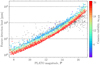 |
Fig. 13 Amplitude detection limit from a prewhitening strategy using the S/N stopping criterion and a high amplitude version of the AFFOGATO SPB sample (cf. Sect. 6.2). This plot illustrates the general noise budget in the frequency domain enforced by random and systematic noise sources. Like in the time domain (see Fig. C.1), the detection limit at mission level is a clear function of the camera observability (colour scale). The dark grey data points are stars with a SPR value larger than 6% (a critical threshold explained in Sect. 6.5). The dotted horizontal lines are reference limits. We highlight that multiple stars have a camera visibility different from nCAM ∈ {6, 12, 18, 24} due to the usage of pointing error sources in our simulations (cf. Sect. 5.1). The same is true for Figs. 14 and 15. While we illustrate the star count histogram (versus nCAM) of this figure in Fig. C.4, the effect in this plot is most noticeable from the four (upper-most) purple/blue data points with nCAM ∈ {1, 2}. |
6.2 Limiting mode amplitude yields
The smallest mode amplitudes detectable as a function of magnitude for each star of the γ Dor and SPB sample are shown in Fig. 14 (left and right panels, respectively), from the simulation batch AFFOGATO (top panels) and CORTADO (bottom panels). First of all, increased scatter is generally observed for CORTADO as compared to AFFOGATO. Secondly, as observed in the time domain, the noise budget of AFFOGATO seems to follow the expected underlying noise model (cf. Fig. 13). On the other hand, the increased level of instrumental systematics of CORTADO clearly impacts the general shape of this distribution, forming a single log-linear relation between 9 < 𝒫 < 13. Using the dotted horizontal lines (at 10 ppm) as references, it is evident that the impact of instrumental systematics enforces that a similar detection limit of AFFOGATO can only be reached if observing a magnitude brighter for CORTADO.
The main differences of the γ Dor and SPB sample is the magnitude distribution (with an upper magnitude cut of 𝒫 = 14 and 𝒫 = 16, respectively) and the mode amplitude distribution (with the SPB stars having generally larger amplitudes). The top right panel of Fig. 14 shows the nominal distribution (of the simulation batch AFFOGATO) constructed from the small Kepler SPB sample of Pedersen et al. (2021). In contrast, a noise plateau exists for the SPB sample for 𝒫 < 9 (top right panel). Similarly, a noise plateau is observed for both the γ Dor and SPB sample of CORTADO (lower left and right panel, respectively). Along each noise plateau, the limiting amplitude detection seems independent of the camera visibility.
The amplitude distribution of the γ Dor sample is expected to be well representative and complete, as it includes all γ Dor stars with identified modes in the Kepler field (Li et al. 2020). On the other hand, the amplitude distribution of the SPB sample is generated from a rather small core sample of stars with excellent seismic information (Pedersen et al. 2021). More recent studies have shown that Gaia too is able to detect g- and p- mode pulsators (see e.g. Gaia Collaboration 2023a; Hey & Aerts 2024). Combining the photometry of TESS and Gaia, Hey & Aerts (2024) discovered thousands of new pulsating stars, across the γ Dor, δ Sct, SPB, β Cep, and hybrid classification, down to a detection threshold of ∼4 ppt. In contradiction to the amplitude distribution recovered from the γ Dor and SPB samples used in this work, Hey & Aerts (2024) found that statistically the two amplitude distributions were not significantly different. While these results are based on the first and second dominant pulsation modes, it is difficult to tell if the true underlying distribution of these two classes of pulsators is in fact identical or distinct, due to the observational biases of Gaia. Moreover, a more pronounced difference in amplitude distribution between the two asteroseismic classes might emerge in PLATO’s passband. Thus, to test how the limiting mode amplitude changes with the injected amplitude distribution, we generated another AFFOGATO batch of simulations with higher mode amplitudes, more in line with Hey & Aerts (2024).
Figure 15 shows a few differences between the high amplitude simulations as compared to the nominal-amplitude simulations: (i) the noise plateau now extends up to 𝒫 ∼ 13; (ii) the lower boundary of the noise plateau has increased to ∼10 ppm and; (iii) the overall scatter has decreased (except in the very faint regime). The former observation is related to a saturation of detectability; left of the dotted vertical lines of Figs. 14 and 15, almost all mode amplitudes are detected. The second observation simply reflects that the smallest amplitudes injected are significantly higher than those of the original sample. The latter observation can readily be understood considering a more precise determination of the mode amplitudes. Meanwhile in the faint end, beyond 𝒫 > 16, the increased scatter is in fact spurious results due to highly contaminated stars (see Fig. 13).
We note that the detection limit presented in Fig. 15 is well aligned with the general PLATO noise budget (see Appendix C). This may reflect that at camera level, in the photon noise limit (𝒫 ≲ 13) the detection limit is independent on magnitude and all pulsation modes can be detected (if the SPR = 0). However, in the sky background/detector noise limit (𝒫 ≳ 13) the pulsation modes start to be increasingly harder to detect, with the detection limit increasing as the square root of the magnitude in agreement with Fig. 13.
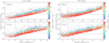 |
Fig. 14 Limiting mode amplitude detection for the γ Dor sample (left panels) and the SPB sample (right panels). Top and bottom panel show the lowest mode amplitude detected for each star of the simulation batch AFFOGATO and CORTADO, respectively. The data points are colour-coded after camera visibility. The dotted horizontal lines are 10 ppm reference lines to compare the two batches. The dotted vertical line in the bottom panel marks a transition between a noise floor plateau (left of line) and an increasing detection limit. |
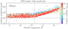 |
Fig. 15 Limiting mode amplitude detection for the SPB sample, simulation batch AFFOGATO, and using an artificially increased mode amplitude distribution. The data points are colour-coded after camera visibility. The dotted vertical line marks a clear transition (at 𝒫 ∼ 12.5) between a noise floor plateau in the bright regime and an increasing detection limit in the faint regime. |
6.3 Mode occurrence rates
To quantify the mode occurrence rates, we calculated the overall yield of detecting oscillation modes of g-mode pulsators as a function of the camera visibility and magnitude (in ∆𝒫 = 1 bins). Figure 16 shows the results of the γ Dor and SPB sample (left and right panels, respectively) for AFFOGATO (top panel), CORTADO (middle panel), and the residuals of the two simulation batches (bottom panel). Again, as expected, the detection rate is steadily decreasing as a function of magnitude and with decreasing camera visibility. As mentioned earlier, looking at the γ Dor sample, for the brightest targets (𝒫 = 8), almost all pulsation modes are detected, with a recovery rate of 93.0–97.5% for AFFOGATO and 81.8–89.3% for CORTADO. However, for the faintest targets (𝒫 = 14), the recovery rates are only 8.8–22.7% for AFFOGATO and 7.2–12.9% for CORTADO. Similar results are recovered from the SPB sample, but with the gradient in the occurrence rate extending to 𝒫 = 16. We note that the mode occurrence rate for 𝒫 < 11 is generally below 50%. This result is particularly promising as it means that the construction of period-spacing patterns, facilitating mode identification, would be possible for a large sample of γ Dor and SPB stars in the LOPS2 (given the 1455 pure g-mode and 1449 hybrid pulsators detected so far within the LOPS2, cf. Hey & Aerts 2024).
The impact of an increased instrumental noise budget of CORTADO compared to AFFOGATO for the γDor and SPB sample is evident from the residual plot in the bottom left and bottom right panels of Fig. 16, respectively. The biggest discrepancy between the two datasets is in the regime 9 < 𝒫 < 13 where the photon noise typically is the dominant noise source. However, the increased dominance of the instrumental systematics (over photon noise) is particularly peaked at 𝒫 ∼ 11 for the γ Dor sample and at 𝒫 ∼ 12 for the SPB sample. Interestingly, the residual trend increases with camera visibility for the γ Dor sample, whereas the opposite is observed for the SPB sample. The former observation is anticipated as a higher level of spacecraft systematics is expected to leave a higher (uncorrected) systematic noise excess in the final light curve when combining uncorrelated observations of more and more cameras. The fact that the two residual distributions disagree indicates that the generally lower mode frequencies of the SPB sample are affected differently by the low frequency systematics than of the γ Dor sample. It is, however, expected to find a smaller yield difference between AFFOGATO and CORTADO for the SPB sample compared to the γ Dor sample, simply due to a smaller impact on the larger mode amplitudes.
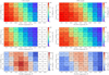 |
Fig. 16 Detection efficiency diagrams (E in %) for the γ Dor sample (left panels) and SPB sample (right panels). The top and middle panels show the detection efficiency as a function of the camera visibility for AFFOGATO and CORTADO, respectively. The bottom panels show the residuals (∆E in %) between the results of AFFOGATO and CORTADO. White boxes marked as ‘nan’ are outside the simulated parameter space. Note a direct comparison is possible between the two samples with respect to the colour scaling. |
6.4 Amplitude and frequency precision
Here, we focus our discussion on the amplitude and frequency precision (cf. Sect. 5.5) of the γ Dor sample, however, the trends are overall the same for the SPB sample. The left panels of Fig. 17 shows the amplitude precision recovery as a function of camera visibility and magnitude. The top and middle panels display the results for AFFOGATO and CORTADO, respectively. The general trend in precision is (as expected) a decreasing function of magnitude and decreasing camera visibility. It is intriguing that an amplitude precision of ≲100 ppm is found below 𝒫 < 12 for both simulation batches. If the two F-CAMs, having respectively a red and blue filter, can reach a similar precision a few orders of magnitudes brighter, this may be excellent news for improved mode identification (e.g. Daszynska-Daszkiewicz 2008; Breger 2014; Reese et al. 2017), which is notoriously hard for massive pulsators (cf. Bowman 2020; Aerts & Tkachenko 2024a).
Similarly to the result seen for the amplitude precision, the frequency precision shown in the right panels of Fig. 17 also shows a decreasing gradient as a function of magnitude and decreasing camera visibility for both AFFOGATO (top panel) and CORTADO (middle panel), respectively. The decreasing trend with decreasing camera visibility is, however, not obvious in the faint limit (e.g. for 𝒫 > 12). Given that generally less than 15% of the pulsation modes could be recovered in the faint regime, an overall frequency precision recovery of ≲10−4 d−1 is a valuable result as forward modelling of high-order g modes requires a frequency precision better than 10−3 d−1 (Aerts et al. 2019).
Looking at the fractional difference in amplitude precision between AFFOGATO and CORTADO (shown in the bottom left panel of Fig. 17) the precision for which the mode amplitudes could be determined does not generally depend much on spacecraft systematics in the bright limit but does so in the faint limit. Comparing this to the fractional difference in frequency precision between AFFOGATO and CORTADO (shown in the bottom right panel of Fig. 17), the largest difference is in the bright limit and the smallest difference is in the faint limit, with a slight dependence on the camera observability. The latter result is rather interesting, as one would generally expect systematics to play an increasing role the more noisy the light curve becomes.
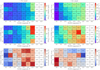 |
Fig. 17 Amplitude precision (left panels; in ppm) and frequency precision (right panels; in d−1) of detected pulsation modes as a function of magnitude and camera visibility for the γ Dor sample. The top and middle panels show the results for AFFOGATO and CORTADO, respectively. The bottom panel shows the fractional residuals between the results of AFFOGATO and CORTADO. Note that compared to all other figures shown in this section, blue indicates the most desirable result. |
6.5 Impact of stellar contamination
Out of 4000 stars, 2650 and 2957 stars (i.e. around 66.3 and 73.9%) from the γ Dor and SPB sample, respectively, have a non-zero stellar pollution ratio (i.e. SPR > 0). Here the SPR represents the average value over all aperture mask definitions from the co-added camera observations.
The simplest case we can consider is flux dilution from nonvariable contaminating stars. Figure 18 explores the relationship between recovered amplitude precision as a function of the SPR and the magnitude for the γ Dor sample (left plots) and as a function of the SPR and the dominant mode amplitude (A1) for the SPB sample (right plots). The top and bottom panels are the results from AFFOGATO and CORTADO, respectively.
Both samples and datasets show a clear correlation between the amplitude precision and the SPR. Most notably is the kink at around 6% third-light level (vertical dotted line), where a drastic increase (i.e. a worsening) of the amplitude precision is observed. While catching almost all spurious outliers of the noise trends shown in Fig. 13, this appears to be a key threshold for on-board PLATO imagery. Additionally, for the dataset AFFOGATO a slight non-linear decreasing trend is observed for increasing SPR values up to the kink, whereas for CORTADO a plateau is observed for the γ Dor sample but less so for the SPB sample. Both the decreasing trend and the local amplitude precision minimum at SPR ∼ 0.06 of AFFOGATO are hard to physically motivate. Hence, it could in fact reflect an optimisation threshold of the optimal aperture mask algorithm itself.
The colour coding in Fig. 18 illustrates that the spread in amplitude precision is related to the brightness (see left plot). For the AFFOGATO simulations (shown for the SPB sample in the right hand plot), this magnitude dependence results in an (well explained) amplitude precision ridge of high A1 modes. On the other hand, for the CORTADO simulations (here only illustrated for the SPB sample), the relation seems only to persevere for the most contaminated stars and wash out stars below the critical SPR threshold. This suggests that instrumental systematics dominate the noise budget up to SPR ∼ 0.06. Thereafter contamination of non-variable stars starts to dominate.
We can further investigate the impact of stellar contamination of non-variable stars in the presence of systematics. The upper and middle panels of Fig. 19 show the residuals of the mode occurrence rates for the γ Dor sample (left plots) and the SPB sample (right plots). Specifically, the upper and lower panels are the residuals between the entire AFFOGATO and CORTADO samples compared to only stars within each sample with SPR > 0, respectively. All four plots show that contamination affects the occurrence rates mostly in the bright regime (i.e. 𝒫 < 11). Moreover, it evident that the stellar contamination in the presence of increased spacecraft systematics has a larger impact on the occurrence rates (decreasing the detection efficiency as expected).
The lower panels of Fig. 19 show the impact of contamination by variable stars (i.e. the batch DOPPIO) for the γ Dor sample (left panel) and the SPB sample (right panel). As compared to results of non-variable contaminants shown in the four upper panels of Fig. 19, the added variability overall washes out the strong gradient of high to low occurrences from the bright to faint regime. Instead, a rather smooth landscape of occurrence rates is observed. Except for a few magnitude/camera visibility configurations, overall the added variability decreases the occurrence rates, making it harder to detect pulsation modes as expected. Lastly, we highlight that instrumental systematics seem to overall decrease the occurrence rates by a factor of two or more, as compared to stellar contamination (variable or not).
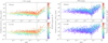 |
Fig. 18 Amplitude precision vs. SPR diagrams for the γ Dor and SPB sample (left and right panels, respectively), and for the simulation batches AFFOGATO and CORTADO (upper and lower panels, respectively). The colour scaling of the γ Dor sample shows the PLATO magnitude and for the SPB sample the dominant mode amplitude (A1). The dotted vertical lines represent a SPR threshold between two amplitude precision regimes. |
6.6 Choice on prewhitening stopping criterion
As a last point of attention, we investigated the difference in results when using either the STAR SHADOW BIC or the standardised S/N prewhitening stopping criterion with respect to the number of input modes. Figure 20 shows the average relative number difference between modes detected with the BIC and S/N threshold as a function of the camera visibility and magnitude.
Considering all samples, it is clear that for AFFOGATO the choice of prewhitening stopping criterion is rather insignificant, with the largest relative difference of detected modes being ∼6.3 and ∼7.5% (corresponding to an actual number difference of ∼1.7 and ∼1.3) for the γDor and SPB samples, respectively. The smallest difference is found in the bright and high nCAM regime, and in the faint and low nCAM regime. This is not surprising since AFFOGATO is dominated by white-noise and the largest discrepancy is approximately in the photon noise dominated regime.
Comparing the results of AFFOGATO to that of CORTADO (middle panels of Fig. 20), the largest relative difference has now increased to ∼11.0 and ∼12.2% (corresponding to an actual number difference of ∼2.8 and ∼2.2) for the γ Dor and SPB samples, respectively. Similar to AFFOGATO, the two samples of CORTADO are generally affected similarly by the choice of the prewhitening strategy. However, as expected, the increased noise budget of CORTADO introduce an offset of around one magnitude towards the bright regime as compared to AFFOGATO.
While the results of the two samples are comparable among AFFOGATO and CORTADO themselves, an offset of around one magnitude for similar recovered values is observed. This is expected as the success of prewhitening depends on the underlying amplitude distribution. The same is true for the frequency distribution due to apodization. However, even for long-cadence PLATO data, the apodization for g-mode pulsators is rather insignificant (e.g. 0.1–1.9% suppression for 1–5 d−1). On a star-to-star basis, more low amplitude modes may be recovered when increasing the FAP for the choice of the S/N. However, given the rather low relative difference in detected modes between the two methods, this is discouraged for larger (statistical) stellar assemblies.
Lastly, we look at the fractional residuals of AFFOGATO and CORTADO for the two samples (lower panels of Fig. 20). A clear trend can be seen towards larger values in the lower left corner (low 𝒫 and high nCAM) and smaller values in the upper right corner (high 𝒫 and low nCAM), with a rather smooth gradient in between. This result shows that the better the photometric precision, the more the instrumental systematics affects the choice of the prewhitening scheme. At first this may be surprising since spurious noise peaks should become increasingly likely to be mistaken for a mode peak in the periodogram. However, the a likely explanation may be that for low 𝒫 and high nCAM, the stellar signal usually dominates over any long-term systematics, resulting in a larger noise floor due to a higher chance of imperfect detrending.
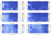 |
Fig. 19 Detection efficiency residual (Δℰ in %) diagrams to test the impact of stellar contamination for the γ Dor sample (left panels) and SPB sample (right panels). The top panels show the results for non-variable targets from AFFOGATO when comparing all stars vs. contaminated stars only. The middle panels show the result for non-variable targets from CORTADO when comparing all stars vs. contaminated stars only. The lower panels show the result considering only contaminated targets and comparing non-variable targets of AFFOGATO vs. variable targets of DOPPIO. Note that the colour scaling of [0, 30] % was chosen in order to make a direct comparison to the Δℰ diagram of CORTADO displayed in the lower panels of Fig. 16. |
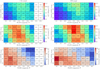 |
Fig. 20 Difference between pulsation mode detected using the BIC and the S/N prewhitening stopping criterion, ΔN = (NBIC − NS/N)/Ninput, as function of magnitude and camera visibility for the γ Dor sample (left panels) and SPB sample (right panels). The top panels show the results for AFFOGATO, the middle panels the result for CORTADO, and the bottom panels show the fractional residuals between AFFOGATO and CORTADO. |
7 Conclusions
In this work, we investigated PLATO’s ability to detect pulsation modes of intermediate-to-massive stars. Despite the fact that the PLATO passband has been optimised for finding transiting exoplanets around solar-type stars, our simulations predict that observing abundant frequency spectra of 𝑔-mode pulsators is achievable with the exquisite long-baseline photometry that PLATO is planning to deliver. For γ Dor and SPB stars, we tested three noise regimes (i.e. AFFOGATO, CORTADO, and DOPPIO cf. Sect. 2) and below we highlight a few key results:
The exact underlying amplitude distribution that will be observed plays a key role in how many modes can be detected and used for asteroseismic modelling. In this work, we used a fully data-driven approach based on Kepler data, as the instability computations tend to be inefficient. Below a limited magnitude of 𝒫 < 14 for the γ Dor sample and 𝒫 < 16 for the SPB sample, the dominant mode amplitude is recovered in more than 95% of the cases, even in the presence of strong residual spacecraft systematics.
The spacecraft systematics increase the noise budget in the photon limited regime of a PLATO observation (9 < 𝒫 < 13). The impact increases the amplitude detection limit with a difference of up to tens of ppm, being equivalent to a difference of around one magnitude in brightness between AFFOGATO and CORTADO in order to reach the same photometric precision.
Throughout the different scenarios for the systematics, the general 𝑔-mode occurrence rates for both samples are above 80% at the bright end and above 6% at the faint end. Furthermore, we find that the g-mode occurrence rate for 𝒫 < 11 is generally above 50%. This highlight that the mode identification using period-spacing patterns would likely be possible for a large sample of γ Dor and SPB stars in LOPS2.
Regarding the mean rms amplitude precision, we find that in most cases, an uncertainty of less than 20 ppm has been retrieved for the γ Dor sample and less than 100 ppm for the SPB sample (with exceptions found for faint targets and low camera visibilities). For the mean rms frequency precision, the uncertainty is always well below the required level of 10−3 d−1 needed for forward asteroseismic modelling (Aerts et al. 2019). Spacecraft systematics affect the amplitude precision mostly for faint targets and low camera visibilities, whereas the opposite is observed for the frequency precision.
Our simulations suggest that stellar contamination does not play a major role for on-board photometry if the third-light contamination is below 6%. Above the 6% level, the amplitude precision is heavily affected, whereas the frequency precision stays almost unaffected. We also showed that stellar contamination from variable stars generally has less of an impact on the yields compared to an increased budget of spacecraft systematics.
We calculated a prewhitening stopping criteria for each PLATO cadence using a significance criterion surface. We showed that there is a difference of ~7% in the number of detected modes when using a classic S/N stopping criterion compared to the BIC stopping criterion. Although the difference is small, the methodology of recovering mode frequencies in this work is biased towards finding pulsations and not noise peaks. Hence, the computed S/N criterion is a safer and more consistent strategy for prewhitening prior to any peak-pattern recognition, as applied to high-order g modes (e.g. Pápics et al. 2014, 2015, 2017; Van Reeth et al. 2015; Li et al. 2020).
While Jannsen et al. (2024) discussed the strengths and shortcomings of PlatoSim, this work presents the most realistic end-to-end simulations for g-mode asteroseismology carried out to date for the PLATO space mission. MOCKA is the first legacy of simulations for PLATO-CS; meanwhile, we plan to perform simulations in the nearby future for each work-package. With PlatoSim continuously being improved, future simulations may for example include a time-dependent model of scattered light from the Earth and the Moon. A more critical milestone for the next-generation simulations is to test PLATO’s reduction pipeline (both on-board and on-ground) with realistic PlatoSim simulations. The expectation is that the PLATO pipeline will provide cleaner light curves as compared to the post-processing pipeline developed for this work.
This work constructs models of oscillations from observational Kepler samples that suffer from observational biases (of their own) to some extent. Moreover, we avoided working with hybrid pulsators in order to unambiguously determine the yield for pure 𝑔-mode pulsators. Despite the theoretical instability regions for pulsators, it is clear that most main sequence stars oscillate and can be hybrid 𝑔- and p-mode pulsators (see Gaia Collaboration 2023a; Hey & Aerts 2024). Thus, future studies may address the added complexity of observing hybrids.
In this project, we did not apply a barycentric correction, which would alter the timings of the 25 s cadence of PLATO. Such irregular but periodically modulated data sampling effectively splits Nyquist aliases into multiplets. Since the shape of these aliases are different from real pulsation frequencies in amplitude spectra, Murphy et al. (2013) showed that for Kepler time series longer than a single orbit around the barycenter, there is no ambiguity in distinguishing between the two. For stars with pulsation frequencies approaching the Nyquist frequency, this will become a problem for increasingly higher frequencies as their amplitudes would steadily reduce due to the irregular sampling. This in turns affects the amplitude S/N and thus the amplitude precision. As the S/N of a mode amplitude depends on the exposure time (Eyer & Bartholdi 1999), we expect the effect to be insignificant for our analysis as the Nyquist frequency is well beyond the highest frequency injected for each sample and the effective exposure time compared to the time sampling for all three PLATO cadences is as high as ∼84%. While this may be irrelevant in the specific context of this project due to a choice of constant cadences, the irregular sampling of PLATO will ultimately allow for super-Nyquist asteroseismology (Murphy et al. 2013).
Although the focus in this work encapsulates the potential for g-mode pulsators on or near the main sequence, MOCKA is an abundant open-source catalogue of pulsators (cf. Table 1) that can be used by the community today. With MOCKA marking the unset to estimate the yield for PLATO as a whole, simulation studies can be performed across multiple complimentary scientific disciplines to uncover the full potential of the mission.
Data availability
All data and appendices are available at: https://doi.org/10.5281/zenodo.14540810
Acknowledgements
This work presents results from the European Space Agency (ESA) space mission PLATO. The PLATO payload, the PLATO Ground Segment and PLATO data processing are joint developments of ESA and the PLATO mission consortium (PMC). Funding for the PMC is provided at national levels, in particular by countries participating in the PLATO Multilateral Agreement (Austria, Belgium, Czech Republic, Denmark, France, Germany, Italy, Netherlands, Portugal, Spain, Sweden, Switzerland, Norway, and United Kingdom) and institutions from Brazil. Members of the PLATO Consortium can be found at https://platomission.com/. The ESA PLATO mission website is https://www.cosmos.esa.int/plato. We thank the teams working for PLATO for all their work. The research behind these results has received funding from the BELgian federal Science Policy Office (BELSPO) through PRODEX grant PLATO: ZKE2050-01-D01. C.A. and M.V. acknowledge financial support from the European Research Council (ERC) under the Horizon Europe programme (Synergy Grant agreement N° 101071505: 4D-STAR). While partially funded by the European Union, views and opinions expressed are however those of the author(s) only and do not necessarily reflect those of the European Union or the European Research Council. Neither the European Union nor the granting authority can be held responsible for them. E.P. has been supported by the ‘SeismoLab’ KKP-137523 Élvonal grant of the Hungarian Research, Development and Innovation Office (NKFIH) and by the NKFIH excellence grant TKP2021- NKTA-64. M.U. gratefully acknowledges funding from the Research Foundation Flanders (FWO) by means of a junior postdoctoral fellowship (grant agreement No. 1247624N). D.M.B. gratefully acknowledges funding from UK Research and Innovation (UKRI) in the form of a Frontier Research grant under the UK government’s ERC Horizon Europe funding guarantee (SYMPHONY; grant number: EP/Y031059/1), and a Royal Society University Research Fellowship (URF; grant number: URF\R1\231631). D.J.F. acknowledges financial support from the Flemish Government under the long-term structural Methusalem funding program by means of the project SOUL: Stellar evolution in full glory, grant METH/24/012 at KU Leuven. L.I.J. acknowledges funding from the Research Foundation Flanders (FWO) under grant agreement 1124321N. M.G.P. acknowledges support from the Professor Harry Messel Research Fellowship in Physics Endowment, at the University of Sydney. R.H. acknowledges support from the German Aerospace Agency (Deutsches Zentrum für Luft- und Raumfahrt) under PLATO Data Center grant 50OO1501. This work has made use of data from the European Space Agency (ESA) mission Gaia (https://www.cosmos.esa.int/gaia), processed by the Gaia Data Processing and Analysis Consortium (DPAC, https://www.cosmos.esa.int/web/gaia/dpac/consortium). Funding for the DPAC has been provided by national institutions, in particular, the institutions participating in the Gaia Multilateral Agreement. This research has made use of NASA’s Astrophysics Data System Bibliographic Services, and the SIMBAD and VizieR databases, operated at CDS, Strasbourg, France. This project additionally made use of the following published Python packages: NumPy (Harris et al. 2020), Numba (Lam et al. 2015), Pandas (McKinney et al. 2011; Reback et al. 2022), SciPy (Virtanen et al. 2020), Matplotlib (Hunter 2007), and Astropy (Astropy Collaboration 2022, 2018, 2013).
References
- Aerts, C. 2021, Rev. Mod. Phys., 93, 015001 [Google Scholar]
- Aerts, C., & Tkachenko, A. 2024a, A&A, 692, R1 [NASA ADS] [CrossRef] [EDP Sciences] [Google Scholar]
- Aerts, C., & Tkachenko, A. 2024b, in 8th TESS/15th Kepler Asteroseismic Science Consortium Workshop, 22 [Google Scholar]
- Aerts, C., Christensen-Dalsgaard, J., & Kurtz, D. W. 2010, Asteroseismology, Springer Science and Business Media (Berlin: Springer) [Google Scholar]
- Aerts, C., Mathis, S., & Rogers, T. M. 2019, ARA&A, 57, 35 [Google Scholar]
- Aigrain, S., Hodgkin, S. T., Irwin, M. J., Lewis, J. R., & Roberts, S. J. 2015, MNRAS, 447, 2880 [NASA ADS] [CrossRef] [Google Scholar]
- Aigrain, S., Parviainen, H., & Pope, B. J. S. 2016, MNRAS, 459, 2408 [NASA ADS] [Google Scholar]
- Antoci, V., Cunha, M., Houdek, G., et al. 2014, ApJ, 796, 118 [Google Scholar]
- Antoci, V., Cunha, M. S., Bowman, D. M., et al. 2019, MNRAS, 490, 4040 [Google Scholar]
- Astropy Collaboration (Robitaille, T. P., et al.) 2013, A&A, 558, A33 [NASA ADS] [CrossRef] [EDP Sciences] [Google Scholar]
- Astropy Collaboration (Price-Whelan, A. M., et al.) 2018, AJ, 156, 123 [Google Scholar]
- Astropy Collaboration (Price-Whelan, A. M., et al.) 2022, AJ, 935, 167 [NASA ADS] [CrossRef] [Google Scholar]
- Auvergne, M., Bodin, P., Boisnard, L., et al. 2009, A&A, 506, 411 [NASA ADS] [CrossRef] [EDP Sciences] [Google Scholar]
- Baran, A. S., & Koen, C. 2021, Acta Astron., 71, 113 [Google Scholar]
- Baran, A. S., Koen, C., & Pokrzywka, B. 2015, MNRAS, 448, L16 [NASA ADS] [CrossRef] [Google Scholar]
- Barragán, O., Aigrain, S., & McCormac, J. 2024, RAS Tech. Instrum., 3, 198 [CrossRef] [Google Scholar]
- Bell, K. J., Córsico, A. H., Bischoff-Kim, A., et al. 2019, A&A, 632, A42 [NASA ADS] [CrossRef] [EDP Sciences] [Google Scholar]
- Blazko, S. 1907, Astron. Nachr., 175, 327 [CrossRef] [Google Scholar]
- Bognár, Z., Kawaler, S. D., Bell, K. J., et al. 2020, A&A, 638, A82 [NASA ADS] [CrossRef] [EDP Sciences] [Google Scholar]
- Bono, G., Braga, V. F., Crestani, J., et al. 2020, ApJ, 896, L15 [NASA ADS] [CrossRef] [Google Scholar]
- Börner, A., Paproth, C., Cabrera, J., et al. 2024, Exp. Astron., 58, 1 [CrossRef] [Google Scholar]
- Borucki, W. J., Koch, D., & Kepler Science Team 2010, AAS/Division for Planetary Sciences Meeting Abstracts, 42, 47.03 [Google Scholar]
- Bouabid, M. P., Dupret, M. A., Salmon, S., et al. 2013, MNRAS, 429, 2500 [Google Scholar]
- Bowman, D. M. 2020, Front. Astron. Space Sci., 7, 70 [Google Scholar]
- Bowman, D. M., & Kurtz, D. W. 2018, MNRAS, 476, 3169 [NASA ADS] [CrossRef] [Google Scholar]
- Bowman, D. M., & Michielsen, M. 2021, A&A, 656, A158 [NASA ADS] [CrossRef] [EDP Sciences] [Google Scholar]
- Bowman, D. M., Kurtz, D. W., Breger, M., Murphy, S. J., & Holdsworth, D. L. 2016, MNRAS, 460, 1970 [NASA ADS] [CrossRef] [Google Scholar]
- Bowman, D. M., Vandenbussche, B., Sana, H., et al. 2022, A&A, 658, A96 [NASA ADS] [CrossRef] [EDP Sciences] [Google Scholar]
- Breger, M. 2014, IAU Symp., 301, 93 [NASA ADS] [Google Scholar]
- Breger, M., Stich, J., Garrido, R., et al. 1993, A&A, 271, 482 [NASA ADS] [Google Scholar]
- Burssens, S., Simón-Díaz, S., Bowman, D. M., et al. 2020, A&A, 639, A81 [NASA ADS] [CrossRef] [EDP Sciences] [Google Scholar]
- Calcaferro, L. M., Sowicka, P., Uzundag, M., et al. 2024, A&A, 686, A140 [NASA ADS] [CrossRef] [EDP Sciences] [Google Scholar]
- Castelli, F., Kurucz, R., Piskunov, N., Weiss, W., & Gray, D. 2003, IAU Symp., 210, A20 [NASA ADS] [Google Scholar]
- Chaplin, W. J., & Miglio, A. 2013, ARA&A, 51, 353 [Google Scholar]
- Chaplin, W. C., Elsworth, Y., Isaak, G. R., et al. 1996, The Observatory, 116, 32 [NASA ADS] [Google Scholar]
- Charpinet, S., Fontaine, G., Brassard, P., & Dorman, B. 1997, Astrophys. Space Sci. Lib., 214, 477 [NASA ADS] [CrossRef] [Google Scholar]
- Choi, J., Dotter, A., Conroy, C., et al. 2016, ApJ, 823, 102 [Google Scholar]
- Chojnowski, S. D., Hubrig, S., Hasselquist, S., et al. 2019, ApJ, 873, L5 [NASA ADS] [CrossRef] [Google Scholar]
- Corsaro, E., Fröhlich, H. E., Bonanno, A., et al. 2013, MNRAS, 430, 2313 [Google Scholar]
- Córsico, A. H., Althaus, L. G., Miller Bertolami, M. M., & Kepler, S. O. 2019, A&A Rev., 27, 7 [Google Scholar]
- Córsico, A. H., Uzundag, M., Kepler, S. O., et al. 2021, A&A, 645, A117 [EDP Sciences] [Google Scholar]
- Córsico, A. H., Uzundag, M., Kepler, S. O., et al. 2022a, A&A, 668, A161 [NASA ADS] [CrossRef] [EDP Sciences] [Google Scholar]
- Córsico, A. H., Uzundag, M., Kepler, S. O., et al. 2022b, A&A, 659, A30 [NASA ADS] [CrossRef] [EDP Sciences] [Google Scholar]
- Cunha, M. S., Aerts, C., Christensen-Dalsgaard, J., et al. 2007, A&A Rev., 14, 217 [Google Scholar]
- Daszynska-Daszkiewicz, J. 2008, Commun. Asteroseismol., 152, 140 [NASA ADS] [CrossRef] [Google Scholar]
- Davenport, J. R. A., Hawley, S. L., Hebb, L., et al. 2014, ApJ, 797, 122 [Google Scholar]
- Davies, G. R., Broomhall, A. M., Chaplin, W. J., Elsworth, Y., & Hale, S. J. 2014, MNRAS, 439, 2025 [Google Scholar]
- Degroote, P., Aerts, C., Baglin, A., et al. 2010, Nature, 464, 259 [Google Scholar]
- De Ridder, J., Telting, J. H., Balona, L. A., et al. 2004, MNRAS, 351, 324 [NASA ADS] [CrossRef] [Google Scholar]
- De Ridder, J., Arentoft, T., & Kjeldsen, H. 2006, MNRAS, 365, 595 [CrossRef] [Google Scholar]
- Duan, R. M., Zong, W., Fu, J. N., et al. 2021, ApJ, 922, 2 [NASA ADS] [CrossRef] [Google Scholar]
- Dupret, M. A., Grigahcène, A., Garrido, R., Gabriel, M., & Scuflaire, R. 2005, A&A, 435, 927 [NASA ADS] [CrossRef] [EDP Sciences] [Google Scholar]
- Dziembowski, W. A., & Pamiatnykh, A. A. 1993, MNRAS, 262, 204 [CrossRef] [Google Scholar]
- Eyer, L., & Bartholdi, P. 1999, A&AS, 135, 1 [NASA ADS] [CrossRef] [EDP Sciences] [Google Scholar]
- Fontaine, G., & Brassard, P. 2008, PASP, 120, 1043 [NASA ADS] [CrossRef] [Google Scholar]
- Fontaine, G., Brassard, P., Charpinet, S., et al. 2012, A&A, 539, A12 [NASA ADS] [CrossRef] [EDP Sciences] [Google Scholar]
- Fritzewski, D. J., Aerts, C., Mombarg, J. S. G., Gossage, S., & Van Reeth, T. 2024a, A&A, 684, A112 [NASA ADS] [CrossRef] [EDP Sciences] [Google Scholar]
- Fritzewski, D. J., Vanrespaille, M., Aerts, C., et al. 2024b, A&A, submitted [arXiv:2408.06097] [Google Scholar]
- Gaia Collaboration (Prusti, T., et al.) 2016, A&A, 595, A1 [NASA ADS] [CrossRef] [EDP Sciences] [Google Scholar]
- Gaia Collaboration (Eyer, L., et al.) 2019, A&A, 623, A110 [NASA ADS] [CrossRef] [EDP Sciences] [Google Scholar]
- Gaia Collaboration (De Ridder, J., et al.) 2023a, A&A, 674, A36 [CrossRef] [EDP Sciences] [Google Scholar]
- Gaia Collaboration (Vallenari, A., et al.) 2023b, A&A, 674, A1 [NASA ADS] [CrossRef] [EDP Sciences] [Google Scholar]
- García, R. A., Hekker, S., Stello, D., et al. 2011, MNRAS, 414, L6 [NASA ADS] [CrossRef] [Google Scholar]
- García, R. A., Mathur, S., Pires, S., et al. 2014, A&A, 568, A10 [Google Scholar]
- Gautschy, A., & Saio, H. 1993, MNRAS, 262, 213 [NASA ADS] [CrossRef] [Google Scholar]
- Gianninas, A., Bergeron, P., & Fontaine, G. 2006, AJ, 132, 831 [NASA ADS] [CrossRef] [Google Scholar]
- Greiss, S., Gänsicke, B. T., Hermes, J. J., et al. 2014, MNRAS, 438, 3086 [NASA ADS] [CrossRef] [Google Scholar]
- Greiss, S., Hermes, J. J., Gänsicke, B. T., et al. 2016, MNRAS, 457, 2855 [CrossRef] [Google Scholar]
- Guzik, J. A., Kaye, A. B., Bradley, P. A., Cox, A. N., & Neuforge, C. 2000, ApJ, 542, L57 [Google Scholar]
- Hale, S. J., Howe, R., Chaplin, W. J., Davies, G. R., & Elsworth, Y. P. 2016, Sol. Phys., 291, 1 [NASA ADS] [CrossRef] [Google Scholar]
- Handberg, R., & Lund, M. N. 2014, MNRAS, 445, 2698 [Google Scholar]
- Handberg, R., Lund, M. N., White, T. R., et al. 2021, AJ, 162, 170 [NASA ADS] [CrossRef] [Google Scholar]
- Harris, W. E. 1996, AJ, 112, 1487 [Google Scholar]
- Harris, C. R., Millman, K. J., van der Walt, S. J., et al. 2020, Nature, 585, 357 [NASA ADS] [CrossRef] [Google Scholar]
- Heber, U. 2009, ARA&A, 47, 211 [Google Scholar]
- Heber, U. 2016, PASP, 128, 082001 [Google Scholar]
- Hekker, S., & Christensen-Dalsgaard, J. 2017, A&A Rev., 25, 1 [NASA ADS] [CrossRef] [Google Scholar]
- Heras, A. M. 2024, EAS, 2024, 2579 [Google Scholar]
- Hermes, J. J., Gänsicke, B. T., Kawaler, S. D., et al. 2017a, ApJS, 232, 23 [Google Scholar]
- Hermes, J. J., Kawaler, S. D., Bischoff-Kim, A., et al. 2017b, ApJ, 835, 277 [Google Scholar]
- Hey, D., & Aerts, C. 2024, A&A, 688, A93 [NASA ADS] [CrossRef] [EDP Sciences] [Google Scholar]
- Heynderickx, D., Waelkens, C., & Smeyers, P. 1994, A&AS, 105, 447 [NASA ADS] [Google Scholar]
- Hippke, M., David, T. J., Mulders, G. D., & Heller, R. 2019, AJ, 158, 143 [Google Scholar]
- Holdsworth, D. L. 2021, Front. Astron. Space Sci., 8, 31 [NASA ADS] [CrossRef] [Google Scholar]
- Holdsworth, D. L., Cunha, M. S., Kurtz, D. W., et al. 2021, MNRAS, 506, 1073 [NASA ADS] [CrossRef] [Google Scholar]
- Holdsworth, D. L., Cunha, M. S., Lares-Martiz, M., et al. 2024, MNRAS, 527, 9548 [Google Scholar]
- Hunter, J. D. 2007, Comput. Sci. Eng., 9, 90 [NASA ADS] [CrossRef] [Google Scholar]
- Husser, T. O., Wende-von Berg, S., Dreizler, S., et al. 2013, A&A, 553, A6 [NASA ADS] [CrossRef] [EDP Sciences] [Google Scholar]
- IJspeert, L. W., Tkachenko, A., Johnston, C., et al. 2021, A&A, 652, A120 [NASA ADS] [CrossRef] [EDP Sciences] [Google Scholar]
- IJspeert, L. W., Tkachenko, A., Johnston, C., et al. 2024, A&A, 685, A62 [NASA ADS] [CrossRef] [EDP Sciences] [Google Scholar]
- Jannsen, N., De Ridder, J., Seynaeve, D., et al. 2024, A&A, 681, A18 [NASA ADS] [CrossRef] [EDP Sciences] [Google Scholar]
- Kallinger, T., De Ridder, J., Hekker, S., et al. 2014, A&A, 570, A41 [NASA ADS] [CrossRef] [EDP Sciences] [Google Scholar]
- Kippenhahn, R., Weigert, A., & Weiss, A. 2013, Stellar Structure and Evolution (Berlin: Springer) [Google Scholar]
- Kjeldsen, H., & Bedding, T. R. 1995, A&A, 293, 87 [NASA ADS] [Google Scholar]
- Koncz, A., Eigmüller, P., Michaelis, H., et al. 2022, SPIE Conf. Ser., 12180, 121801E [NASA ADS] [Google Scholar]
- Kurtz, D. W., Saio, H., Takata, M., et al. 2014, MNRAS, 444, 102 [Google Scholar]
- Lam, S. K., Pitrou, A., & Seibert, S. 2015, in Proc. Second Workshop on the LLVM Compiler Infrastructure in HPC, 1 [Google Scholar]
- Li, G., Van Reeth, T., Bedding, T. R., et al. 2020, MNRAS, 491, 3586 [Google Scholar]
- Loi, S. T. 2020, MNRAS, 496, 3829 [Google Scholar]
- Lomb, N. R. 1976, Ap&SS, 39, 447 [Google Scholar]
- Luger, R., Agol, E., Kruse, E., et al. 2016, AJ, 152, 100 [Google Scholar]
- Lund, M. N., Handberg, R., Davies, G. R., Chaplin, W. J., & Jones, C. D. 2015, ApJ, 806, 30 [NASA ADS] [CrossRef] [Google Scholar]
- Lund, M. N., Handberg, R., Buzasi, D. L., et al. 2021, ApJS, 257, 53 [NASA ADS] [CrossRef] [Google Scholar]
- Marchiori, V., Samadi, R., Fialho, F., et al. 2019, A&A, 627, A71 [NASA ADS] [CrossRef] [EDP Sciences] [Google Scholar]
- Mathis, S., Bugnet, L., Prat, V., et al. 2021, A&A, 647, A122 [EDP Sciences] [Google Scholar]
- Mathys, G., Kurtz, D. W., & Holdsworth, D. L. 2020, A&A, 639, A31 [NASA ADS] [CrossRef] [EDP Sciences] [Google Scholar]
- Maxted, P. F. L., Ehrenreich, D., Wilson, T. G., et al. 2022, MNRAS, 514, 77 [NASA ADS] [CrossRef] [Google Scholar]
- McKinney, W., et al. 2011, Python for High Performance and Scientific Computing (USA: ACM Digital Library), 14, 1 [Google Scholar]
- McNamara, D. H., & Barnes, J. 2014, AJ, 147, 31 [Google Scholar]
- Meunier, N., Lagrange, A. M., Boulet, T., & Borgniet, S. 2019, A&A, 627, A56 [NASA ADS] [CrossRef] [EDP Sciences] [Google Scholar]
- Miglio, A., Montalbán, J., Noels, A., & Eggenberger, P. 2008, MNRAS, 386, 1487 [Google Scholar]
- Molnár, L., Bódi, A., Pál, A., et al. 2022, ApJS, 258, 8 [CrossRef] [Google Scholar]
- Mombarg, J. S. G., Van Reeth, T., Pedersen, M. G., et al. 2019, MNRAS, 485, 3248 [NASA ADS] [CrossRef] [Google Scholar]
- Mombarg, J. S. G., Rieutord, M., & Espinosa Lara, F. 2024, A&A, 683, A94 [NASA ADS] [CrossRef] [EDP Sciences] [Google Scholar]
- Montalto, M., Piotto, G., Marrese, P. M., et al. 2021, A&A, 653, A98 [NASA ADS] [CrossRef] [EDP Sciences] [Google Scholar]
- Montgomery, M. H., & O’Donoghue, D. 1999, Delta Scuti Star Newsletter, 13, 28 [NASA ADS] [Google Scholar]
- Moravveji, E., Townsend, R. H. D., Aerts, C., & Mathis, S. 2016, ApJ, 823, 130 [NASA ADS] [CrossRef] [Google Scholar]
- Mukadam, A. S., Mullally, F., Nather, R. E., et al. 2004, ApJ, 607, 982 [NASA ADS] [CrossRef] [Google Scholar]
- Munari, M., Magrin, D., Ragazzoni, R., et al. 2022, SPIE Conf. Ser., 12180, 121804I [Google Scholar]
- Murphy, S. J., Shibahashi, H., & Kurtz, D. W. 2013, MNRAS, 430, 2986 [NASA ADS] [CrossRef] [Google Scholar]
- Murphy, S. J., Hey, D., Van Reeth, T., & Bedding, T. R. 2019, MNRAS, 485, 2380 [NASA ADS] [CrossRef] [Google Scholar]
- Nascimbeni, V., Piotto, G., Börner, A., et al. 2022, A&A, 658, A31 [NASA ADS] [CrossRef] [EDP Sciences] [Google Scholar]
- Nascimbeni, V., Piotto, G., Cabrera, J., et al. 2025, A&A, in press, https://doi.org/10.1051/0004-6361/202452325 [Google Scholar]
- Offner, S. S., Moe, M., Kratter, K. M., et al. 2022, arXiv e-prints [arXiv:2203.10066] [Google Scholar]
- Oliveira da Rosa, G., Kepler, S. O., Córsico, A. H., et al. 2022, ApJ, 936, 187 [NASA ADS] [CrossRef] [Google Scholar]
- Østensen, R. H., Bloemen, S., Vuckovic, M., et al. 2011, ApJ, 736, L39 [CrossRef] [Google Scholar]
- Ouazzani, R.-M., Salmon, S. J. A. J., Antoci, V., et al. 2017, MNRAS, 465, 2294 [Google Scholar]
- Ouazzani, R. M., Marques, J. P., Goupil, M. J., et al. 2019, A&A, 626, A121 [NASA ADS] [CrossRef] [EDP Sciences] [Google Scholar]
- Pápics, P. I., Moravveji, E., Aerts, C., et al. 2014, A&A, 570, A8 [NASA ADS] [CrossRef] [EDP Sciences] [Google Scholar]
- Pápics, P. I., Tkachenko, A., Aerts, C., et al. 2015, ApJ, 803, L25 [Google Scholar]
- Pápics, P. I., Tkachenko, A., Van Reeth, T., et al. 2017, A&A, 598, A74 [Google Scholar]
- Pascual-Granado, J., Suárez, J. C., Garrido, R., et al. 2018, A&A, 614, A40 [NASA ADS] [CrossRef] [EDP Sciences] [Google Scholar]
- Pedersen, M. G. 2022, ApJ, 940, 49 [NASA ADS] [CrossRef] [Google Scholar]
- Pedersen, M. G., Aerts, C., Pápics, P. I., et al. 2021, Nat. Astron., 5, 715 [NASA ADS] [CrossRef] [Google Scholar]
- Penoyre, Z., Belokurov, V., Wyn Evans, N., Everall, A., & Koposov, S. E. 2020, MNRAS, 495, 321 [NASA ADS] [CrossRef] [Google Scholar]
- Pertenais, M., Cabrera, J., Paproth, C., et al. 2021, SPIE Conf. Ser., 11852, 118524Y [NASA ADS] [Google Scholar]
- Plachy, E., Pál, A., Bódi, A., et al. 2021, ApJS, 253, 11 [NASA ADS] [CrossRef] [Google Scholar]
- Rauer, H., Catala, C., Aerts, C., et al. 2014, Exp. Astron., 38, 249 [Google Scholar]
- Rauer, H., Aerts, C., Cabrera, J., et al. 2024, arXiv e-prints [arXiv:2406.05447] [Google Scholar]
- Reback, J., McKinney, W., Van Den Bossche, J., et al. 2022, https://doi.org/10.5281/zenodo.7344967 [Google Scholar]
- Reese, D. R., Lignières, F., Ballot, J., et al. 2017, A&A, 601, A130 [NASA ADS] [CrossRef] [EDP Sciences] [Google Scholar]
- Renson, P., & Manfroid, J. 2009, A&A, 498, 961 [NASA ADS] [CrossRef] [EDP Sciences] [Google Scholar]
- Ricker, G. R., Winn, J. N., Vanderspek, R., et al. 2015, J. Astron. Telesc. Instrum. Syst., 1, 014003 [Google Scholar]
- Romero, A. D., Kepler, S. O., Hermes, J. J., et al. 2022, MNRAS, 511, 1574 [NASA ADS] [CrossRef] [Google Scholar]
- Romero, A. D., da Rosa, G. O., Kepler, S. O., et al. 2023, MNRAS, 518, 1448 [Google Scholar]
- Royer, P., Baeke, A., Terrasa, G., et al. 2022, SPIE Conf. Ser., 12180, 121804H [Google Scholar]
- Rui, N. Z., & Fuller, J. 2023, MNRAS, 523, 582 [NASA ADS] [CrossRef] [Google Scholar]
- Rybizki, J., Green, G. M., Rix, H.-W., et al. 2022, MNRAS, 510, 2597 [NASA ADS] [CrossRef] [Google Scholar]
- Saio, H., Kurtz, D. W., Takata, M., et al. 2015, MNRAS, 447, 3264 [Google Scholar]
- Samadi, R., Deru, A., Reese, D., et al. 2019, A&A, 624, A117 [NASA ADS] [CrossRef] [EDP Sciences] [Google Scholar]
- Scargle, J. D. 1982, ApJ, 263, 835 [Google Scholar]
- Schönrich, R., McMillan, P., & Eyer, L. 2019, MNRAS, 487, 3568 [Google Scholar]
- Shibahashi, H. 1979, PASJ, 31, 87 [NASA ADS] [Google Scholar]
- Stankov, A., & Handler, G. 2005, ApJS, 158, 193 [NASA ADS] [CrossRef] [Google Scholar]
- Stellingwerf, R. F. 1984, ApJ, 277, 322 [Google Scholar]
- Sun, J. Q., Cheng, X., Ding, M. D., et al. 2015, Nat. Commun., 6, 7598 [CrossRef] [Google Scholar]
- Tassoul, M. 1980, ApJS, 43, 469 [Google Scholar]
- Tkachenko, A., Aerts, C., & Jannsen, N. 2024, EAS, 2024, 871 [Google Scholar]
- Tovar Mendoza, G., Davenport, J. R. A., Agol, E., Jackman, J. A. G., & Hawley, S. L. 2022, AJ, 164, 17 [CrossRef] [Google Scholar]
- Udalski, A., Szymanski, M., Kaluzny, J., Kubiak, M., & Mateo, M. 1992, Acta Astron., 42, 253 [NASA ADS] [Google Scholar]
- Udalski, A., Szymanski, M. K., Soszynski, I., & Poleski, R. 2008, Acta Astron., 58, 69 [NASA ADS] [Google Scholar]
- Udalski, A., Szymanski, M. K., & Szymanski, G. 2015, Acta Astron., 65, 1 [Google Scholar]
- Uzundag, M., Córsico, A. H., Kepler, S. O., et al. 2021, A&A, 655, A27 [NASA ADS] [CrossRef] [EDP Sciences] [Google Scholar]
- Uzundag, M., Córsico, A. H., Kepler, S. O., et al. 2022, MNRAS, 513, 2285 [NASA ADS] [CrossRef] [Google Scholar]
- Uzundag, M., De Gerónimo, F. C., Córsico, A. H., et al. 2023, MNRAS, 526, 2846 [NASA ADS] [CrossRef] [Google Scholar]
- Uzundag, M., Krzesinski, J., Pelisoli, I., et al. 2024, A&A, 684, A118 [NASA ADS] [CrossRef] [EDP Sciences] [Google Scholar]
- Van Beeck, J., Prat, V., Van Reeth, T., et al. 2020, A&A, 638, A149 [NASA ADS] [CrossRef] [EDP Sciences] [Google Scholar]
- Van Beeck, J., Bowman, D. M., Pedersen, M. G., et al. 2021, A&A, 655, A59 [NASA ADS] [CrossRef] [EDP Sciences] [Google Scholar]
- Vanderburg, A., & Johnson, J. A. 2014, PASP, 126, 948 [Google Scholar]
- Van Doorsselaere, T., Shariati, H., & Debosscher, J. 2017, ApJS, 232, 26 [NASA ADS] [CrossRef] [Google Scholar]
- Van Reeth, T., Tkachenko, A., Aerts, C., et al. 2015, A&A, 574, A17 [NASA ADS] [CrossRef] [EDP Sciences] [Google Scholar]
- Van Reeth, T., Tkachenko, A., & Aerts, C. 2016, A&A, 593, A120 [NASA ADS] [CrossRef] [EDP Sciences] [Google Scholar]
- Van Reeth, T., Mombarg, J. S. G., Mathis, S., et al. 2018, A&A, 618, A24 [NASA ADS] [EDP Sciences] [Google Scholar]
- Virtanen, P., Gommers, R., Oliphant, T. E., et al. 2020, Nat. Methods, 17, 261 [Google Scholar]
- Voss, B., Koester, D., Østensen, R., et al. 2006, A&A, 450, 1061 [NASA ADS] [CrossRef] [EDP Sciences] [Google Scholar]
- Walker, G., Matthews, J., Kuschnig, R., et al. 2003, PASP, 115, 1023 [Google Scholar]
- Winget, D. E., & Kepler, S. O. 2008, ARA&A, 46, 157 [Google Scholar]
- Zhang, J., Fu, J., Cang, T., et al. 2024, ApJ, 976, 46 [Google Scholar]
- Zong, W., Charpinet, S., Vauclair, G., Giammichele, N., & Van Grootel, V. 2016, A&A, 585, A22 [NASA ADS] [CrossRef] [EDP Sciences] [Google Scholar]
- Zong, W., Charpinet, S., & Vauclair, G. 2021, ApJ, 921, 37 [NASA ADS] [CrossRef] [Google Scholar]
https://github.com/IvS-KULeuven/PlatoSim3 (for PLATO mission consortium members).
Due to the direct usage of pulsation modes of RR Lyrae and Cepheid (cf. Sects. 4.1.5 and 4.1.6), the light curve asymmetry is preserved. While some high amplitude δ Sct and β Cep stars also show strongly asymmetric light curves (e.g. Bowman et al. 2016; Stankov & Handler 2005), we do not model these stellar minorities in this work.
The PC can also be determined in a model independent way using concomitant light curves from multiple instruments (e.g. Bowman et al. 2016).
Related to data gaps, in principle any large movement of the spacecraft (e.g. quarterly rotations, safe mode events, etc.) will introduce small thermal changes across the payload (affecting mounts, optics, and detectors), which gradually relaxes typically on time scales from hours to days. Seen as exponential decaying structures in the extracted light curve, these so-called ‘thermal transients’ are caused by an increased detector gain or/and general PSF breathing. Due to PLATO’s aperture mask strategy this may have a significant effect on the onboard photometry, hence, we acknowledge their importance for future simulations.
All Tables
All Figures
|
Fig. 1 Illustration of the first PLATO pointing field called LOPS2. The platform pointing (being parallel to the pointing of the two F- CAMs; see magenta star) is centred at the equatorial coordinate (α, δ) = (95.310 43°, −47.886 93°), with zero rotation with respect to the Galactic equator. The N-CAM overlap of nCAM ∈ {6,12,18,24} is illustrated with an increasing darker shade of blue (also indicated in the white boxes), and the blue, green, yellow, and red dot show the pointing of N-CAM group one, two, three, and four, respectively. The black transparent map highlights dense sky regions such as the location of the Milky Way plane, the Large Magellanic Cloud (LMC, encircled in orange), and a few globular clusters (pink circles, from Harris 1996). |
| In the text | |
|
Fig. 2 CaMD of stars from the LOPS2 (see Fig. 1) within 1 kpc from the Sun. Here, G, GBP, and GRP refer to the Gaia full-bandwidth, blue, and red passband, respectively. Commonly known CaMD features are highlighted with coloured text. Each of the coloured circles indicates the approximate region of a stellar pulsation class that is a part of MOCKA. |
| In the text | |
|
Fig. 3 HRD of the γ Dor and SPB (left panel), and δ Sct and β Cep (right panel) stellar samples. The colour gradient indicates the stellar surface gravity, and over-plotted are MIST evolutionary tracks (Choi et al. 2016). Solid lines indicate instability strips for gravity modes in the left panel and pressure modes in the right panel. The red lines show the edges of the theoretical γ Dor instability strip from Dupret et al. (2005) (corresponding to a mixing length of respectively αMLT = 2 (solid lines) and αMLT = 1.5 (dashed lines) in the left-hand plot). The orange lines represent the observational δ Sct instability strip from Murphy et al. (2019). The blue and purple lines are the theoretical instability regions of SPB and β Cep stars, respectively, calculated by Burssens et al. (2020). |
| In the text | |
|
Fig. 4 Model fit to the gradient–period relation for dipole sectoral prograde g modes from Li et al. (2020). Typically this diagram features the mean period, but here we correlate the first mode period in the period spacing pattern with the gradient. The colour scaling shows the value of the corresponding first period spacing. |
| In the text | |
|
Fig. 5 Example of a simulated SPB star. The lower/left axes belong to the amplitude spectrum (blue line), where we have highlighted the mode frequencies (dotted lines), the first mode period (P0), and the first period spacing (ΔP0). The upper/right axes belong to the corresponding light curve (shown for the first 15 days) in its noise-less form (orange line) and simulated form (black points, representing a 𝓟 ≈ 10.3 star observed with nCAM = 6). |
| In the text | |
|
Fig. 6 Power spectral density (PSD) diagrams showing granulation and pulsation signals caused by large convective envelopes in low-mass dwarfs. The PSD was computed for a 2-yr noise-less light curve. The bottom panel is a zoom-in on the combined model illustrating the standard envelope of excited modes (used to estimate the frequency of maximum power, νmax) and the small (δv) and large (Δv) frequency separations. |
| In the text | |
|
Fig. 7 Illustration of a stellar on-axis activity model for a solar-like star simulated for two years. (a) Spot emergence diagram with the black dots being their latitudinal location and relative sizes at emergence with respect to the stellar surface. (b) Stellar surface area covered by spots (in percentage). (c) Relative flux darkening by the spot coverage (in ppt) as function time. (d) Relative flux brightening by stellar flares (in ppt) as function of time. |
| In the text | |
|
Fig. 8 Gaussian KDE distribution per spectral type of the LOPS2–Gaia DR3 single stars with valid stellar bulk parameters. The normalised density is scaled from low to high with brown to purple colour, respectively. A cut in the density region, discarding the lowest 25–50%, has been made to each spectral type to better confine each region. |
| In the text | |
|
Fig. 9 CaMD of different stellar classes used to assign a variable signal to stellar contaminants. The respective class is written in the title header together with the number count of the class. The upper panels show the confinement of all stars that feature solar-like variability: (a) red giants, (b) solar-like dwarfs and subgiants, and (c) red dwarfs. The lower panels show the confinement of (d) binaries, (e) giants and compact objects (above the purple line and below the blue lines, respectively), and (f) all objects with an unknown spectral type. The black points are all stars in the LOPS2 (G ≲ 17), whereas the metallic contour defines stars within 1 kpc from the Sun. |
| In the text | |
|
Fig. 10 Assembly of data gaps included prior to the frequency analysis. Besides the quarterly rotational realignment of the spacecraft (blue lines), we also consider downtime due to station keeping manoeuvres (purple lines), loss of fine guidance (orange lines), and safe mode events (red lines). |
| In the text | |
|
Fig. 11 Histogram of the S/N of the highest amplitude frequency extracted from 10 000 synthetic white noise PLATO light curves. This example shows the optimal S/N criterion (dashed lines) estimated as the FAP = 1% from time series with a duration of eight mission quarters. |
| In the text | |
|
Fig. 12 Optimum significance surface for PLATO light curves with a cadence of δt = 25 s. The surface fit was performed with Eq. (9) to the grid points (sorted in colour after the FAP, with semi-regular grid points of {10, 8,6,4,2, 1, 0.5, 0.1, 0.01}%). |
| In the text | |
|
Fig. 13 Amplitude detection limit from a prewhitening strategy using the S/N stopping criterion and a high amplitude version of the AFFOGATO SPB sample (cf. Sect. 6.2). This plot illustrates the general noise budget in the frequency domain enforced by random and systematic noise sources. Like in the time domain (see Fig. C.1), the detection limit at mission level is a clear function of the camera observability (colour scale). The dark grey data points are stars with a SPR value larger than 6% (a critical threshold explained in Sect. 6.5). The dotted horizontal lines are reference limits. We highlight that multiple stars have a camera visibility different from nCAM ∈ {6, 12, 18, 24} due to the usage of pointing error sources in our simulations (cf. Sect. 5.1). The same is true for Figs. 14 and 15. While we illustrate the star count histogram (versus nCAM) of this figure in Fig. C.4, the effect in this plot is most noticeable from the four (upper-most) purple/blue data points with nCAM ∈ {1, 2}. |
| In the text | |
|
Fig. 14 Limiting mode amplitude detection for the γ Dor sample (left panels) and the SPB sample (right panels). Top and bottom panel show the lowest mode amplitude detected for each star of the simulation batch AFFOGATO and CORTADO, respectively. The data points are colour-coded after camera visibility. The dotted horizontal lines are 10 ppm reference lines to compare the two batches. The dotted vertical line in the bottom panel marks a transition between a noise floor plateau (left of line) and an increasing detection limit. |
| In the text | |
|
Fig. 15 Limiting mode amplitude detection for the SPB sample, simulation batch AFFOGATO, and using an artificially increased mode amplitude distribution. The data points are colour-coded after camera visibility. The dotted vertical line marks a clear transition (at 𝒫 ∼ 12.5) between a noise floor plateau in the bright regime and an increasing detection limit in the faint regime. |
| In the text | |
|
Fig. 16 Detection efficiency diagrams (E in %) for the γ Dor sample (left panels) and SPB sample (right panels). The top and middle panels show the detection efficiency as a function of the camera visibility for AFFOGATO and CORTADO, respectively. The bottom panels show the residuals (∆E in %) between the results of AFFOGATO and CORTADO. White boxes marked as ‘nan’ are outside the simulated parameter space. Note a direct comparison is possible between the two samples with respect to the colour scaling. |
| In the text | |
|
Fig. 17 Amplitude precision (left panels; in ppm) and frequency precision (right panels; in d−1) of detected pulsation modes as a function of magnitude and camera visibility for the γ Dor sample. The top and middle panels show the results for AFFOGATO and CORTADO, respectively. The bottom panel shows the fractional residuals between the results of AFFOGATO and CORTADO. Note that compared to all other figures shown in this section, blue indicates the most desirable result. |
| In the text | |
|
Fig. 18 Amplitude precision vs. SPR diagrams for the γ Dor and SPB sample (left and right panels, respectively), and for the simulation batches AFFOGATO and CORTADO (upper and lower panels, respectively). The colour scaling of the γ Dor sample shows the PLATO magnitude and for the SPB sample the dominant mode amplitude (A1). The dotted vertical lines represent a SPR threshold between two amplitude precision regimes. |
| In the text | |
|
Fig. 19 Detection efficiency residual (Δℰ in %) diagrams to test the impact of stellar contamination for the γ Dor sample (left panels) and SPB sample (right panels). The top panels show the results for non-variable targets from AFFOGATO when comparing all stars vs. contaminated stars only. The middle panels show the result for non-variable targets from CORTADO when comparing all stars vs. contaminated stars only. The lower panels show the result considering only contaminated targets and comparing non-variable targets of AFFOGATO vs. variable targets of DOPPIO. Note that the colour scaling of [0, 30] % was chosen in order to make a direct comparison to the Δℰ diagram of CORTADO displayed in the lower panels of Fig. 16. |
| In the text | |
|
Fig. 20 Difference between pulsation mode detected using the BIC and the S/N prewhitening stopping criterion, ΔN = (NBIC − NS/N)/Ninput, as function of magnitude and camera visibility for the γ Dor sample (left panels) and SPB sample (right panels). The top panels show the results for AFFOGATO, the middle panels the result for CORTADO, and the bottom panels show the fractional residuals between AFFOGATO and CORTADO. |
| In the text | |
Current usage metrics show cumulative count of Article Views (full-text article views including HTML views, PDF and ePub downloads, according to the available data) and Abstracts Views on Vision4Press platform.
Data correspond to usage on the plateform after 2015. The current usage metrics is available 48-96 hours after online publication and is updated daily on week days.
Initial download of the metrics may take a while.