| Issue |
A&A
Volume 691, November 2024
|
|
|---|---|---|
| Article Number | A131 | |
| Number of page(s) | 13 | |
| Section | Stellar structure and evolution | |
| DOI | https://doi.org/10.1051/0004-6361/202451651 | |
| Published online | 05 November 2024 | |
Estimates of (convective core) masses, radii, and relative ages for ∼14 000 Gaia-discovered gravity-mode pulsators monitored by TESS
1
IRAP, Université de Toulouse, CNRS, UPS, CNES, 14 Avenue Édouard Belin, F-31400 Toulouse, France
2
Institute of Astronomy, KU Leuven, Celestijnenlaan 200D, B-3001 Leuven, Belgium
3
Université Paris-Saclay, Université de Paris, Sorbonne Paris Cité, CEA, CNRS, AIM, 91191 Gif-sur-Yvette, France
4
Department of Astrophysics, IMAPP, Radboud University Nijmegen, PO Box 9010 6500 GL Nijmegen, The Netherlands
5
Max Planck Institute for Astronomy, Königstuhl 17, 69117 Heidelberg, Germany
6
Institute for Astronomy, University of Hawai’i, Honolulu, HI, 96822
USA
⋆ Corresponding authors; This email address is being protected from spambots. You need JavaScript enabled to view it.
; This email address is being protected from spambots. You need JavaScript enabled to view it.
Received:
25
July
2024
Accepted:
4
October
2024
Abstract
Context. Gravito-inertial asteroseismology saw its birth from the 4-year-long light curves of rotating main-sequence stars assembled by the Kepler space telescope. High-precision measurements of internal rotation and mixing are available for about 600 stars of intermediate mass so far that are used to challenge the state-of-the-art stellar structure and evolution models.
Aims. Our aim is to prepare for future large ensemble modelling of gravity-mode pulsators by relying on a new sample of such stars recently discovered from the third Data Release of the Gaia space mission and confirmed by space photometry from the TESS mission. This sample of potential asteroseismic targets is about 23 times larger than the Kepler sample.
Methods. We use the effective temperature and luminosity inferred from Gaia to deduce evolutionary masses, convective core masses, radii, and ages for ∼14 000 gravity-mode pulsators classified as such from their nominal TESS light curves. We do so by constructing two dedicated grids of evolutionary models for rotating stars with input physics from the asteroseismic calibrations of Keplerγ Dor pulsators. These two grids consider the distribution of initial rotation velocities at the zero-age main sequence deduced from gravito-inertial asteroseismology, for two extreme values found for the metallicity of γ Dor stars deduced from spectroscopy ([M/H]=0.0 and −0.5).
Results. We find the new gravity-mode pulsators to cover an extended observational instability region covering masses from about 1.3 M⊙ to about 9 M⊙. We provide their mass-luminosity and mass-radius relations, as well as convective core masses. Our results suggest that oscillations excited by the opacity mechanism occur uninterruptedly for the mass range above about 2 M⊙, where stars have a radiative envelope aside from thin convection zones in their excitation layers.
Conclusions. Our evolutionary parameters for the sample of Gaia-discovered gravity-mode pulsators with confirmed modes by TESS offer a fruitful starting point for future TESS ensemble asteroseismology once a sufficient number of modes is identified in terms of the geometrical wave numbers and overtone for each of the pulsators.
Key words: asteroseismology / methods: numerical / stars: evolution / stars: fundamental parameters / stars: interiors / stars: oscillations
© The Authors 2024
 Open Access article, published by EDP Sciences, under the terms of the Creative Commons Attribution License (https://creativecommons.org/licenses/by/4.0), which permits unrestricted use, distribution, and reproduction in any medium, provided the original work is properly cited.
This article is published in open access under the Subscribe to Open model. This email address is being protected from spambots. You need JavaScript enabled to view it. to support open access publication.
1. Introduction
Data Release 3 (DR3, Gaia Collaboration 2023a) of the ESA Gaia space mission (Gaia Collaboration 2016a,b, 2018) contains the time-series photometry of millions of variable stars classified and delivered by Coordination Unit 7 (CU 7, Eyer et al. 2023). Even if the mission was not specifically designed for it, Gaia’s sparsely sampled DR3 photometric light curves revealed excellent capacity to discover a multitude of new nonradial pulsators. In particular, Gaia Collaboration (2023b, hereafter called Paper I) discovered more than 100 000 of such pulsators occurring along the main sequence, where a variety of excitation mechanisms are known to be active (Aerts et al. 2010, Chapter 2).
In a follow-up study to Paper I, Aerts et al. (2023, hereafter Paper II) considered the more than 15 000 newly discovered Gaia DR3 candidate gravity (g-)mode pulsators. These turned out to have a dominant amplitude above about 4 mmag, which was found to mark the detection threshold for nonradial oscillations with significant frequencies occurring in the sparse DR3 light curves. The CU 7 algorithms assigned these pulsators to either the class of Slowly Pulsating B-type stars (SPB stars hereafter, Waelkens 1991; Waelkens et al. 1998; Aerts et al. 1999; De Cat & Aerts 2002) or the class of γ Doradus stars (γ Dor stars hereafter, Kaye et al. 1999; Handler 1999; Uytterhoeven et al. 2011). Both these classes consist of multiperiodic low-frequency (typically between 0.5 d−1 and 3 d−1) g-mode pulsators with internal rotation frequencies covering from slow to very fast compared to the frequencies of the excited modes (Pápics et al. 2017; Aerts et al. 2019; Li et al. 2020).
Since the era of high-cadence space photometry started, thousands of pulsators have been discovered from their high-precision (down to μmag) uninterrupted space photometric light curves. These are mainly assembled with the NASA Kepler and Transiting Exoplanet Survey Satellite (TESS) space telescopes (see Kurtz 2022, for an extensive review). Even though thousands of g-mode pulsators were discovered from Kepler data (Blomme et al. 2010; Debosscher et al. 2011; Uytterhoeven et al. 2011), only about 700 were characterised asteroseismically so far (Li et al. 2020; Pedersen et al. 2021; Aerts 2021 for a summary), because this requires proper identification of the mode geometry of several g modes per star. While frequency analysis methods from high-cadence light curves are well established (Aerts et al. 2010, Chapter 5) and easy to apply (e.g. Bowman 2017; Van Beeck et al. 2021), identification of the corresponding mode geometry for each of the significant frequencies is not a straightforward task. For g modes, such identification can be established from the detection of so-called period spacing patterns revealed by modes of consecutive radial overtone, as highlighted in the theory papers by Miglio et al. (2008), Bouabid et al. (2013) and Van Reeth et al. (2015a). This potential was first put into practice for two SPB stars monitored during five months by the CoRoT mission (Degroote et al. 2010; Pápics et al. 2012).
The real breakthrough in g-mode asteroseismology of main-sequence stars came from the 4-year-long Kepler light curves. These data opened up the new sub-field of gravito-inertial asteroseismology (e.g. Pápics et al. 2014; Van Reeth et al. 2015a,b, 2016; Van Reeth et al. 2018; Moravveji et al. 2015, 2016; Schmid & Aerts 2016; Ouazzani et al. 2017; Szewczuk & Daszyńska-Daszkiewicz 2018; Wu et al. 2018; Wu & Li 2019; Mombarg et al. 2019, 2021; Ouazzani et al. 2019; Li et al. 2020, 2024; Sekaran et al. 2021; Pedersen et al. 2021; Szewczuk et al. 2021, 2022; Pedersen 2022a,b; Fritzewski et al. 2024a,b). This led to the major conclusion that single intermediate-mass stars have nearly rigid rotation throughout the long core-hydrogen burning phase of their evolution, with levels of differentiality between the near-core region and the stellar surface typically below 10% (Li et al. 2020). The same conclusion holds for rotation frequencies of the core (Saio et al. 2021). These findings required revisions of the stellar evolution theory of such stars in regards to the transport of angular momentum (Aerts et al. 2019; Fuller et al. 2019; Moyano et al. 2024).
The excitation of g modes in SPB stars is linked to the κ-mechanism, operating around the iron opacity peak in the partial ionisation zone of heavy elements such as iron and nickel at a temperature of about 200 kK. This mechanism drives an efficient heat-engine cycle, exciting slow eigenmodes with periods of about one day to a couple of days. In γ Dor stars, the dominant excitation mechanism is believed to be convective flux blocking. This mechanism operates at the interface between the radiative zone and the thin convective outer envelope, situated in an area with a temperature from about 200 kK to 500 kK (Guzik et al. 2000; Dupret et al. 2005). However, convective flux blocking alone cannot explain the observed hotter γ Dor stars, suggesting that the κ-mechanism also plays a role in these stars (Xiong et al. 2016). The current commonly used instability regions for the SPB stars (Szewczuk & Daszyńska-Daszkiewicz 2017) and γ Dor stars (Dupret et al. 2005) suggest a gap between the red edge of the SPB instability region and the blue edge of the γ Dor strip, even when considering time-dependent convection and adopting a range of mixing-length parameters. Yet, g-mode pulsators are observed to fall within this gap (Balona & Ozuyar 2020; Balona 2024, and Paper I) indicating that at least some of the astrophysical properties of these stars are still not fully captured by the models and/or the theory of mode excitation.
In this paper, we estimate masses, convective core masses, radii, and ages (in terms of the central hydrogen-mass fraction) of the largest sample of g-mode pulsators so far. We investigate their properties from the dominant oscillation mode discovered in the Gaia DR3 data and meanwhile confirmed by the TESS space photometry (Hey & Aerts 2024). Combining the information in these space photometric light curves allows us to map the instability regions more carefully than has been done so far and to decide whether there is indeed a lack of stars with excited g modes in the mass regime between roughly 2 and 3 M⊙. We discuss the main astrophysical properties of the ∼14 000 Gaia DR3 g-mode pulsators confirmed and reclassified as such from TESS photometry. We also provide their potential for future asteroseismic forward and inverse modelling.
Section 2 treats the sample selection while Sect. 3 focuses on our modelling approach, which is based on two grids of stellar models, one for solar metallicity and one for a metallicity of [M/H] = −0.5. Section 4 covers the derived parameters, including the mass, convective core mass, radius, and age. We end the paper with our conclusions in Sect. 5.
2. Sample selection
It was shown in Paper II that the Gaia DR3 candidate g-mode pulsators have similar properties as the genuine SPB or γ Dor pulsators observed with the Kepler space telescope, which delivered 4-year-long high-cadence μmag-precision light curves (Gilliland et al. 2010; Kurtz 2022). This resemblance not only concerned their fundamental parameters, but also the dominant frequency and its amplitude. Nevertheless, these similarities are not a solid proof that the candidate pulsators identified by Paper I are genuine class members, because the Gaia DR3 data only delivered one or two significant frequencies. Moreover, the Fourier Transforms of the Gaia DR3 light curves reveal instrumental frequencies at mmag level, particularly for frequencies above the satellite spinning frequency of about 4 d−1. Regardless whether most of the gravito-inertial modes in SPB and γ Dor stars occur below this satellite frequency, it is difficult to exclude that the secondary frequencies in the Gaia DR3 light curves deduced in Paper I originate from the satellite instead of from the target stars.
In order to confirm (or refute) the nature of the Gaia DR3 candidate pulsators, Hey & Aerts (2024) considered high-cadence light curves assembled by the nominal TESS mission (having a time base between 27 d and 352 d). They relied on all the candidate pulsators found in Paper I having data available in the homogeneously reduced TESS–Gaia light curve (TGLC) catalogue produced from full-frame images by Han & Brandt (2023). A total of 58 970 stars out of the 106 207 Gaia DR3 candidate pulsators classified in Paper I have TGLC light curves. Analyses of this data revealed that more than 70% of the 58 970 stars have the same dominant frequency in the completely independent TGLC and Gaia DR3 light curves. Moreover, Hey & Aerts (2024) reported that almost all these stars turn out to be genuine multiperiodic pulsators.
A reclassification of these 58 970 TESS-confirmed pulsators was performed by Hey & Aerts (2024). Here, we take all stars they classified as γ Dor/SPB or hybrid pulsator with more than two observed significant independent frequencies in the TESS data. This selection criterion is based on earlier classification work for highly sampled photometric light curves assembled from space. Debosscher et al. (2009) and Blomme et al. (2010) showed that a classifier based on the demand of having at least three independent frequencies is very effective in selecting γ Dor pulsators from space photometry (Tkachenko et al. 2013; Van Reeth et al. 2015b).
For our study, we wish to maximise the sample size of Gaiag-mode pulsators. However, we do not want to include too many contaminants according to the confusion matrix of the random forest classifier used by Hey & Aerts (2024). Aside from demanding three significant frequencies, which greatly helps to avoid eclipsing binaries or rotational variables, we inspect the properties of the dominant frequency commonly present in the Gaia and TESS photometry. Figure 1 shows this frequency, its amplitude, and also the total number of significant frequencies in the nominal TESS light curve as a function of the classification probability from Hey & Aerts (2024). We achieved maximal ranges of frequencies and amplitudes at Ppred ≃ 0.5. For this reason, we worked with the sample of stars having Ppred ≥ 0.5.
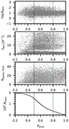 |
Fig. 1. Pulsational characteristics of the sample. From top to bottom: amplitude of dominant frequency in the TESS light curve (in mmag), dominant frequency, and number of significant frequencies in the nominal TESS data. The bottom panel shows the number of stars above a given threshold on the classification probability Ppred from Hey & Aerts (2024). Vertical dashed lines indicate the used threshold in Ppred for the different samples. |
Furthermore, we eliminated pulsators whose effective temperature locates them outside the two grids of stellar models discussed in Sect. 3. This resulted in a total of ∼14 000 new confirmed Gaia DR3 g-mode pulsators, 13 682 stars when we assume a metallicity of [M/H]= − 0.5, and 14 072 stars when we assume [M/H]=0, to be exact. We also investigated the effect of using a lower threshold Ppred ≥ 0.2 and a higher threshold Ppred ≥ 0.8, on the probability of the star being a g-mode or hybrid pulsator, which yielded a total of 18 132 (18 634) and 3165 (3195) stars, respectively for [M/H]= − 0.5 (0.0). These numbers include cuts that we impose to exclude stars that fall outside of the used grids of stellar models, as we will discuss later.
The ∼14 000 stars with Ppred ≥ 0.5 of being a g-mode pulsator cover one global observational instability region as shown in Fig. 2. This observational ‘combined Gaia-DR3/TESS’ g-mode instability strip is far more extended than the joint coverage of various theoretically predicted individual strips for SPB and γ Dor stars computed by assuming that these pulsators are excited by convective flux blocking or the κ mechanism. This was already found in Paper I from Gaia DR3 data and also independently concluded from a summary of high-cadence Kepler and TESS space photometry by Balona (2024). We discuss the distributions of the properties of the pulsators, including the effect of the chosen threshold in the classification probability on our results.
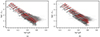 |
Fig. 2. Hertzsprung-Russell diagrams showing the sample of g-mode pulsators with Ppred ≥ 0.5 (grey symbols with error bars). The evolutionary tracks show the extend of the grid of rotating stellar models, covering a mass range of [1.3, 9] M⊙, where the black (red) colour indicates ω0 = 0.05 (0.55), and the solid (dashed) line style fCBM = 0.005 (0.025). |
The Gaia DR3 sample of stars having a probability above 50% to be a g-mode pulsator from TESS is 23 times larger than the Kepler sample of 611 γ Dor stars that were asteroseismically characterised by Li et al. (2020). Starting from this Kepler sample, Fritzewski et al. (2024b) and Mombarg et al. (2024) determined the mass, convective core mass, radius, and age from grid-based modelling for subsets of respectively 490 and 539 of these pulsators, restricting to targets with identified prograde dipole modes and their measured asymptotic period spacing Π0, also known as the buoyancy radius, or buoyancy travel time as it has the dimensions of a period. On the other hand, Li et al. (2020) estimated the internal rotation frequency near the convective core from the slope of the measured period spacing patterns from dipole prograde modes of consecutive radial order for all 611 genuine Keplerγ Dor stars with such identified modes. For the Gaiag-mode pulsators, we cannot perform asteroseismic modelling at this stage because their modes are not identified in terms of their geometry. This opportunity may occur in the future from their 5-year (or longer) yearly-interrupted TESS photometry. So far, such mode identification has only been achieved for stars in the Continuous Viewing Zones of TESS (Garcia et al. 2022a,b; Fritzewski et al. 2024a; Li et al. 2024).
Our aim for now is to prepare for future asteroseismic ensemble modelling of the Gaia-discovered TESS-confirmed g-mode pulsators by already deducing initial estimates for their masses, radii, convective core masses, and ages from the homogeneously deduced Gaia DR3 data. We do so for ∼14 000 new Gaia/TESS g-mode pulsators classified as such by Hey & Aerts (2024) with a probability above 50% and having the same dominant frequency in both independent light curves. To reach our goal, we relied on their Gaia DR3 effective temperature and luminosity (obtained from the GSP-Phot analysis, Paper I), which are two observables available for all stars in the sample, thus allowing us to do a homogeneous sample analysis. To compensate for the generally underestimated uncertainties on the effective temperature, we inflated the uncertainties by a factor 3. This way, the typical uncertainty is more in line with what is achieved with high-resolution spectroscopy (Gebruers et al. 2021), namely a median uncertainty of 108 K. The average relative uncertainty as a function of the effective temperature itself is constant, while for logL/L⊙, there is a decrease from ∼8% to ∼3% between 1 < logL/L⊙ < 2. We coupled these observables to two grids of stellar evolution models for rotating stars. These models have been constructed specifically for our purpose, by relying on input physics calibrated by the genuine Keplerγ Dor prograde dipole pulsators from asteroseismic modelling by Mombarg (2023). These models are compliant with the observed angular momentum of the stellar interior as probed by gravito-inertial asteroseismology following the method in Aerts et al. (2018) and summarised in Aerts (2021).
3. Grid-based parameter estimation
Our parameter estimation relies on the effective temperature and luminosity from Gaia DR3 as the two observables. These were coupled to the theoretically predicted values as derived from two grids of stellar evolution models with input physics calibrated by gravito-inertial asteroseismology. We first describe these model grids and then the method of the parameter estimation. Our computational setup, computed models, and results discussed below are publicly available on Zenodo1.
3.1. Stellar structure and evolution models
We compute a grid of stellar structure and evolution models with the code MESA r24.03.1 (Paxton et al. 2011, 2013, 2015; Paxton et al. 2018, 2019; Jermyn et al. 2023) covering masses, M⋆, between 1.3 and 9 M⊙. We assume an exponentially decaying convective-boundary mixing (CBM, or overshoot) zone outside the convective core, where the radiative temperature gradient is taken and for which the slope of the diffusion coefficient with respect to the radial coordinate is set by a factor fCBM times the local pressure scale height. We varied this parameter for each stellar mass between 0.005 and 0.025, based on the inferred distributions from the sample of 539 genuine Keplerγ Dor stars by Mombarg et al. (2024). The switch from convective mixing to CBM was set to a distance of 0.005 times the local pressure scale height into the convection zone (overshoot_f0 in MESA). We also varied the initial fraction of Keplerian critical rotation at the zero-age main sequence (ZAMS), ω0, (assuming a uniform rotation profile at the ZAMS) between 5 and 55%, following Mombarg et al. (2024). In MESA, the stellar structure equations are modified when rotation is enabled by redefining the radius coordinate, r, such that a sphere with this radius has the same volume as the distorted surface in the Roche model. This assumes that the angular velocity, Ω, is constant over isobars.
The chemical diffusion coefficient in the radiative envelope was computed from the rotational mixing predicted by the theoretical works of Zahn (1992) and Chaboyer & Zahn (1992),
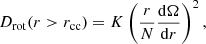 (1)
(1)
where K is the thermal diffusivity, N the Brunt-Väisälä frequency, and rcc the radius of the convective core. The transport of angular momentum is done in a fully diffusive implementation, where we assumed a constant viscosity equal to 107 cm2 s−1. This is consistent with the range derived for slowly rotating γ Dor stars near the terminal-age main sequence (TAMS) (Mombarg 2023). The evolution of a model is stopped if critical rotation is reached. This happens for a handful of models only.
We note that it is currently not well known which processes drive chemical mixing inside the radiative envelopes of main-sequence stars with a convective core. This is why we mimicked the unknown internal mixing processes and their effect on the luminosity and the effective temperature by encompassing the CBM parameter (fCBM). Furthermore, we did not include microscopic diffusion, but note that this type of mixing alters the local Rosseland mean opacity. We compute this opacity for a solar mixture according to Asplund et al. (2009) using the data from the Opacity Project (Seaton 2005).
Adopting the present-day cosmic abundances of nearby early B-type stars from Nieva & Przybilla (2012) as initial composition, we compute a first grid of models for a metallicity Z = 0.014. This places many of the stars below the ZAMS line (Fig. 2, right panel). While the error bars based on the Gaia data are rather uncertain, this finding may represent shortcomings in the physics during the contraction phase until the ZAMS (we refer to Zwintz & Steindl 2022 for an extensive discussion). However, the position of the stars below the ZAMS for solar metallicity is also in line with the sub-solar metallicity found consistently from both high-resolution ground-based spectroscopy and Gaia spectroscopy of γ Dor stars obtained by Gebruers et al. (2021) and de Laverny et al. (2024), respectively. For this reason, we also compute a second grid of models, for a metallicity Z = 0.0045 ([M/H] = −0.5) found as lower limit for a large sample of γ Dor stars by de Laverny et al. (2024) from Gaia spectroscopy. This second grid gives better agreement with the Gaia data as most stars are now well positioned above the ZAMS line (Fig. 2, left panel). For the grid with Z = 0.014, an initial helium mass fraction of Y = 0.2612 was used, and for the Z = 0.0045 grid Y = 0.2495 was used, following the chemical enrichment rate derived by Verma et al. (2019). The parameter ranges covered by the grids are listed in Table 1. We limited ourselves to a lower limit of 1.3 M⊙, since none of the g-mode pulsators known to date has a mass below this value. Moreover, lower-mass models require a different treatment of rotation as magnetic breaking becomes important.
Parameter range covered by the grids used to train the CNF.
Convection is treated following mixing length theory (Cox & Giuli 1968), where we use the solar-calibrated value αMLT = 1.8 (Choi et al. 2016). Since stars in the mass range considered here do not have a significant convective envelope during the main sequence, and we rely on models calibrated from gravity modes probing the deep interior, our work does not depend on the exact choice of αMLT. Furthermore, an Eddington grey atmosphere is assumed, with an opacity that is consistent with the local temperature and pressure of the atmosphere.
3.2. Interpolation with conditional normalising flows
We seek to interpolate the computed stellar evolution models in the three aforementioned physical quantities, M⋆, fCBM, and ω0. The potential of conditional normalising flows (CNFs) to emulate grids of stellar models has been pointed out by Hon et al. (2024), to which we refer for details on the methodology. In brief, normalising flows represent a class of probabilistic machine learning tools with the capacity to make transformations between simple and more complex distributions. Here, we take a similar approach as presented by Hon et al. (2024), making use of the Zuko software package (Rozet et al. 2023).
The general principle of normalising flows is to train a neural network to learn the transformation for a simple probability distribution of a random variable z to a more complex distribution of a variable y = f(z). The transformation can be conditioned based on labels c such that probability densities p(y|c) can be estimated. The labels c (conditional variables) are in this case M⋆, fCBM, and ω0. The output variables are the effective temperature (Teff, in log scale), the luminosity (L⋆/L⊙, in log scale), the rotation rate measured by the g modes at the convective core boundary (Ωgc), the hydrogen mass fraction in the core compared to the initial one (Xc/Xini), the mass of the convective core (mcc/M⊙), and the stellar radius (R⋆/R⊙, in log scale). The CNF is trained on a data set of ∼155 000 points representing the evolution models in each grid.
We draw 2.5 million samples from the trained CNF within the ranges of M⋆, fCBM, and ω0 covered by the grid of stellar models. The combination of these three conditional variables are sampled uniformly. To avoid oversampling near the ZAMS and TAMS, we resample from these 2.5 million points such that we are left with a more or less uniform initial distribution of Xc/Xini values. This leaves us with at least one million samples. For each star in the sample, the likelihood of each sample drawn from the CNF is computed,
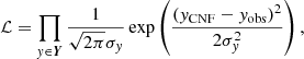 (2)
(2)
where σy denotes the observational uncertainty, and Y = {logTeff, logL/L⊙}. We then compute weighted kernel density estimations (KDE) for M⋆, Xc/Xini, mcc/M⋆, and logR⋆/R⊙, where the likelihood values are taken as the weights. The optimal KDE bandwidth is determined using the Silverman method (Silverman 1986). The uncertainties are defined as the 68% confidence interval. We discard stars that clearly fall outside the grid by imposing cuts at 3.81 < logTeff < 4.43 and logL/L⊙ < 5.2logTeff − 18.3.
4. Derived evolutionary stellar parameters
Figure 3 shows the resulting KDEs of the maximum likelihood estimates (MLEs) of the inferred masses, the evolutionary stages (Xc/Xini) as a proxy for the ages, the convective core masses, and the radii. We show the results for the three different probability thresholds of the classification results in Hey & Aerts (2024). We leave out stars that fall in either the lowest or the highest mass bin, as we consider them to be located outside the grid. Combined with the cuts mentioned above, this omits 748 stars for Z = 0.0045 and 373 stars for Z = 0.014 (Ppred ≥ 0.5).
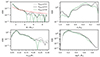 |
Fig. 3. Kernel density estimations of the MLEs for the stellar mass (top-left), the fraction of initial hydrogen in the core (top-right), the fractional core mass (bottom-left), and the stellar radius (bottom-right), assuming Z = 0.0045. The different colours indicate different threshold on the classification probability from Hey & Aerts (2024) for the star to be considered a g-mode pulsator. The red line in the top-left panel corresponds to a Salpeter IMF with dN/dM ∝ M−2.35. |
Two-sample Kolomogorov-Smirnov tests are performed to determine whether a different threshold in Ppred affects the underlying distributions of the inferred stellar parameters. We adopt as null hypothesis that the underlying distributions of both samples are equal and reject it for p values lower than 0.05. We find that the distributions for M⋆, Xc/Xini, mcc/M⋆ are not drawn for the same underlying distribution for the samples based on Ppred = 0.2 and Ppred = 0.5 (see Table 2). Yet, for the distribution of the radius, the null hypothesis cannot be rejected. When we omit stars above 4 M⊙, as higher masses are under-sampled, the null hypothesis can also not be rejected for the distribution of Xc/Xini. Furthermore, two-sample Kolomogorov-Smirnov tests for the distributions of Ppred = 0.5 and Ppred = 0.8 yield p values lower than 0.05 for all four inferred stellar parameters. These conclusions hold for both Z = 0.0045 and Z = 0.014. We do caution over-interpretation of these tests because the sample sizes are quite different (Fig. 1).
Summary of p values from two-sample Kolomogorov-Smirnov tests.
We estimate the uncertainty of the derived distributions by means of bootstrapping, where each measurement is perturbed independently within its uncertainty interval following a uniform probability2. The results of 1000 iterations are shown in grey in Fig. 4. We conclude that the shape of the derived distributions is robust, although the uncertainties at higher masses are larger as a result of the scarcity of higher-mass g-mode pulsators. The derived distribution of the stellar masses is compared with a Salpeter initial-mass function (IMF, Salpeter 1955) dN/dM ∝ M−2.35. We observe an excess of g-mode pulsators below roughly 1.6 M⊙. This suggests that the convective flux blocking mechanism is efficient in exciting g modes within a narrow mass range.
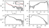 |
Fig. 4. Same as Fig. 3, but for Ppred ≥ 0.5 (in black) and the result of 1000 iterations of bootstrapping (in grey). The inset in the top-left panel shows a zoom-in around the mass range of γ Dor pulsators. |
Interestingly, we do not observe a drop in the number of g-mode pulsators between the predicted blue edge of the γ Dor instability region (roughly above 2 M⊙, Dupret et al. 2005) and the predicted red edge of the SPB instability region (roughly below 3 M⊙, Szewczuk & Daszyńska-Daszkiewicz 2017). We perform one-sample Kolomogorov-Smirnov tests assuming a cumulative distribution function predicted by a Salpeter IMF. We adopt as null hypothesis that the sample is drawn from the assumed IMF distribution. Again, we omit stars with a mass above 4 M⊙ to avoid under-representation. When using a variable lower limit on the stellar mass and a fixed upper limit of 4 M⊙, we find that the mass distribution of our sample of g-mode pulsators is compatible with a Salpeter IMF down to roughly 2.2−2.5 M⊙, even for the strict threshold of Ppred ≥ 0.8, as shown in Fig. 5. The resulting deduced mass distribution of the Gaia pulsators therefore indicates that the κ-mechanism is effective in exciting g modes between the currently assumed disjoint theoretical instability regions of γ Dor and SPB stars.
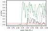 |
Fig. 5. Resulting p value from a one-sample Kolomogorov-Smirnov test between the inferred mass distribution of the sample of g-mode pulsators and a Salpeter IMF, as a function of the mass range tested. The upper mass is always 4 M⊙. The solid lines correspond to Z = 0.0045, the dashed lines correspond to Z = 0.014. The solid red line indicates a p value of 0.05 below which we reject the null hypothesis. |
As already highlighted in the Introduction, observational evidence for pulsators in this part of the Hertzsprung-Russell diagram (HRD) had already been found from high-cadence space photometry assembled with the Kepler and TESS space telescopes, prior to the results from Gaia DR3 by Gaia Collaboration (2023b) and Aerts et al. (2023), and Hey & Aerts (2024). Even earlier Mowlavi et al. (2013, 2016) detected fast rotating g-mode pulsators with dominant amplitudes of a few mmag in that part of the HRD of a young open cluster, while Degroote et al. (2009) detected many candidate pulsators in that region from CoRoT space photometry as well. Along with the summary by Balona (2024) it seems firmly established now that g-mode pulsations occur all along the main sequence. Our results on the mass distribution are in line with these earlier observational studies.
The distribution of masses within the γ Dor range has a similar shape compared to the mass distribution derived by Mombarg et al. (2024) for the 539 genuine γ Dor stars observed by the Kepler mission. We do, however, find a peak in the number of stars around 1.4 M⊙ (top-left panel in Fig. 4), which is slightly lower in mass than the peak around ∼1.5 M⊙ observed for the Kepler prograde dipole g-mode pulsators considered by Mombarg et al. (2024). Furthermore, we observe a clear relation between the inferred mass and the observed luminosity, with log(L⋆/L⊙)=4.0623(6)log(M⋆/M⊙)+0.3468(2) as shown in Fig. 6. This is a somewhat steeper mass–luminosity relation than the one found by Yakut et al. (2007) based on eclipsing binaries with a B-type star component, namely log(L⋆/L⊙)=3.724log(M⋆/M⊙)+0.162. This is understood in terms of the increased importance of the radiation pressure with respect to the ideal gas law in the equation of state when going from F-type stars to B-type stars.
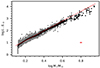 |
Fig. 6. Relation between the inferred stellar mass and the measured luminosity from Gaia of the stars in the sample. The solid red line indicates the fitted mass-luminosity relation, yielding log(L⋆/L⊙)=4.0623(6)log(M⋆/M⊙)+0.3468(2). The black triangles indicate bin averaged-values. Average uncertainties are indicated by the red data point. |
We find the majority of stars to form a plateau around 40% of their initial hydrogen mass fraction left in the convective core, with a shape of a broad normal distribution around this peak value. The fact that most stars appear to be mid-main sequence is dominated by the γ Dor stars in the parameter region where convective flux blocking is active.
The bottom-left panel of Fig. 4 shows the distributions of the fractional convective core masses (mcc/M⋆). The peak originates from the fact that the sample contains both stars having an initially growing convective core and stars with purely receding cores during the main sequence. We show the correlation between the mass of the convective core and total stellar mass in Fig. 7. The solid black and red lines show the maximum convective core mass as a function of total mass occurring in the grid, for CMB with fCBM = 0.005 and fCBM = 0.025, respectively. The dashed lines show the location for about half the main sequence, that is, at Xc/Xini = 0.4. We see that numerous stars occur between the black and red lines, which reveals that a fraction of γ Dor stars with a mass below ∼1.8 M⊙ experience some level of CBM. However, most stars have a convective core mass below the maximum for modest CBM (fCBM = 0.005), as was also found by Mombarg et al. (2024) for the genuine Keplerγ Dor sample. The maximum convective core mass of stars above roughly 2 M⊙ is not dependent on the CBM efficiency for the range of values we considered in our grids, but we recall that we excluded envelope mixing in our model grids while this may be an important ingredient to deduce the convective core mass of SPB stars (Pedersen et al. 2021; Pedersen 2022a). Asteroseismic modelling of oscillation frequencies is required to evaluate the cumulative effect of envelope mixing.
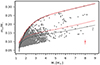 |
Fig. 7. Relation between the inferred stellar mass and fractional convective core mass of the stars in the sample. The solid black (red) line indicates the maximum core mass possible during the main sequence for fCBM = 0.005 (0.025). The dashed lines show the maximum core mass at Xc/Xini = 0.4 (same colour coding). Average uncertainties are indicated by the red data point. |
The bottom-right of Fig. 4 shows the distributions of the inferred stellar radii. Figure 8 shows the mass against the radius. As is common, we find more scatter in the mass–radius relation than in the mass–luminosity relation. We perform a fit with two linear components, where we place the knee at logM⋆/M⊙ = 0.3 (2 M⊙), as stars below this mass are less inflated because they have a thin outer convective layer, while those with a higher mass have a fully radiative envelope. This yields R⋆ ∝ M⋆1.469(3) on the lower-mass end, and R⋆ ∝ M⋆0.380(4) on the higher-mass end, where the knee is located at logR⋆/R⊙ = 0.4609(5).
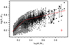 |
Fig. 8. Relation between the inferred stellar mass and the inferred stellar radius (from models) of the stars in the sample. The solid red line indicates a two-component linear fit to the data (see text). The black triangles indicate bin averaged-values. Average uncertainties are indicated by the red data point. |
In Fig. 9 (and Fig. A.3 for Z = 0.014), we show the derived correlation between the evolutionary stage (via Xc/Xini) and the convective-core mass. In this figure, we only show stars above 2 M⊙, as the γ Dor stars are not equally sampled in mass for each bin in Xc/Xini, since the more massive ones tend to be closer to the TAMS, while the less massive ones are closer to the ZAMS. The downward trend of the core mass over time observed in Fig. 9 is consistent with a constant value of fCBM along the main sequence, as can be seen from the models shown in this figure. However, variations in the value of fCBM along the main sequence between the most extreme values used in our grids cannot be ruled out. While we do appreciate that the trend shown in Fig. 9 is to some extent enforced by the physics of the evolution models used, we note that this physics is based on detailed asteroseismic modelling studies (e.g. Pedersen et al. 2021; Michielsen et al. 2021; Burssens et al. 2023; Mombarg et al. 2024).
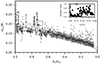 |
Fig. 9. Relation between the inferred fraction Xc/Xini and the convective core mass for stars M⋆ > 2 M⊙. The black triangles indicate the average per bin and standard deviation. Two models are shown for 2.4 M⊙ and ω0 = 0.05, where the mass is representative of the median stellar mass per bin as shown in the inset. The black colour corresponds to fCBM = 0.005, the red colour to fCBM = 0.025. |
We repeat the exercise with a CNF trained on the grid with Z = 0.014. The results for the stars with Ppred ≥ 0.5 are shown in Fig. 10. Our conclusions are qualitatively the same for this grid modelling keeping in mind a tight mass-metallicity relation, except that we now see an excess of stars that fall below the ZAMS line. Using this assumption of the metallicity, we obtain a mass-luminosity relation log(L⋆/L⊙)=4.1825(5)log(M⋆/M⊙)+0.1057(2). For the mass-radius relation we find R⋆ ∝ M⋆1.740(3) on the lower-mass end, and R⋆ ∝ M⋆0.623(3) on the higher-mass end, where the knee is located at logR/R⊙ = 0.3945(3). The corresponding figures are shown in Appendix A. We expect most stars to have a true metallicity between the two extremes considered here. The more metal-poor models give better consistency for the observed pulsators as a population above the ZAMS based on the Gaia effective temperatures and luminosities, while their membership to the thin disk of the Milky Way would advocate for a more solar composition (see de Laverny et al. 2024, for a detailed discussion). We quantify the effect of assuming an incorrect metallicity in Appendix B.
5. Conclusions
In this paper, we have made use of conditional normalising flows trained on two grids of rotating one-dimensional stellar evolution models calibrated by asteroseismology of γ Dor stars. Using this method, we derived masses, evolutionary stages (on the main sequence), convective core masses, and radii of ∼14 000 new galactic g-mode pulsators. These form an all-sky sample and were discovered from sparse Gaia DR3 light curves. All stars were confirmed to be multiperiodic pulsators from TESS nominal high-cadence space photometry (Hey & Aerts 2024). This sample of TESS-confirmed g-mode main-sequence pulsators offers an increase with more than a factor 23 compared to the Kepler sample of asteroseismically modelled main-sequence g-mode pulsators.
The parameter determination we provide here is based on the stars’ effective temperature and luminosity only, and hence represents evolutionary parameters. These estimates cannot be compared with parameters deduced from detailed asteroseismic modelling, but they offer initial estimates from the homogeneously treated Gaia DR3 data. The two observables for each star were coupled to a grid of stellar evolution models constructed with input physics deduced from the sample of 611 asteroseismically calibrated Keplerγ Dor pulsators covering rotation rates from almost zero to almost the critical rate. The homogeneously determined (convective core) masses and radii offer a valuable starting point for future ensemble asteroseismic modelling of these g-mode pulsators, once a sufficient number of their modes can be identified from high-cadence TESS or future PLATO (Rauer et al. 2024) space photometry.
Biases in the effective temperature of GSP-Phot used in this work might be present. The study by Avdeeva et al. (2024) report systematically higher effective temperatures measured by GSP-Phot compared those of the APOGEE survey. The largest discrepancies between GSP-Phot and APOGEE are, however, reported for BP − RP values between 2 and 4.5 mag, whereas the stars in our sample have BP − RP < 1.5. A potential systematic overestimation of the effective temperature by GSP-Phot would lead to overestimated stellar masses and underestimated values for Xc/Xini. On the other hand, Avdeeva et al. (2024) show that the effective temperatures from GSP-Phot and the GALAH survey are globally in good agreement (limited to effective temperatures below 8000 K). Asteroseismic effective temperatures will be inferred from follow-up studies of this sample and may shed light on the systematics.
The distributions of stellar masses of the sample of g-mode pulsators are in general agreement with a Salpeter IMF, except that we find an excess of stars within the mass range of the γ Dor pulsators. This suggests that flux blocking at the bottom of the thin convective envelope is a highly effective excitation mechanism for g-mode oscillations (Guzik et al. 2000; Dupret et al. 2005). On the other hand, g-mode excitation by the κ-mechanism seems to occur effectively in stars covering masses from about 2 M⊙ to about 9 M⊙, but our sample is not representative for the stars with a mass above 4 M⊙. As long as we do not have the full lists of detected identified oscillation modes per star, we cannot make more detailed inferences on the effectivity of the excitation mechanisms in terms of particular modes. Such inferences will be the subject of further studies.
Note that the resulting distributions of the MLEs do not necessarily follow a normal distribution. Therefore, we take the more conservative assumption to sample from a uniform distribution within the 68%-confidence interval.
Acknowledgments
We thank the anonymous referee for the suggestions that have improved the presentation of our results. JSGM acknowledges funding the French Agence Nationale de la Recherche (ANR), under grant MASSIF (ANR-21-CE31-0018-02). The research leading to these results has received funding from the KU Leuven Research Council (grant C16/18/005: PARADISE) and from the European Research Council (ERC) under the Horizon Europe programme (Synergy Grant agreement N°101071505: 4D-STAR). While partially funded by the European Union, views and opinions expressed are however those of the authors only and do not necessarily reflect those of the European Union or the European Research Council. Neither the European Union nor the granting authority can be held responsible for them. This research has made use of the Numpy (van der Walt et al. 2011), Scipy (Virtanen et al. 2020) and Matplotlib (Hunter 2007) software packages.
References
- Aerts, C. 2021, Rev. Mod. Phys., 93, 015001 [Google Scholar]
- Aerts, C., De Cat, P., Peeters, E., et al. 1999, A&A, 343, 872 [NASA ADS] [Google Scholar]
- Aerts, C., Christensen-Dalsgaard, J., & Kurtz, D. W. 2010, Asteroseismology (Heidelberg: Springer-Verlag) [Google Scholar]
- Aerts, C., Molenberghs, G., Michielsen, M., et al. 2018, ApJS, 237, 15 [Google Scholar]
- Aerts, C., Mathis, S., & Rogers, T. M. 2019, ARA&A, 57, 35 [Google Scholar]
- Aerts, C., Molenberghs, G., & De Ridder, J. 2023, A&A, 672, A183 [NASA ADS] [CrossRef] [EDP Sciences] [Google Scholar]
- Asplund, M., Grevesse, N., Sauval, A. J., & Scott, P. 2009, ARA&A, 47, 481 [NASA ADS] [CrossRef] [Google Scholar]
- Avdeeva, A. S., Kovaleva, D. A., Malkov, O. Y., & Zhao, G. 2024, MNRAS, 527, 7382 [Google Scholar]
- Balona, L. A. 2024, ApJ, submitted [arXiv:2310.09805] [Google Scholar]
- Balona, L. A., & Ozuyar, D. 2020, MNRAS, 493, 5871 [CrossRef] [Google Scholar]
- Blomme, J., Debosscher, J., De Ridder, J., et al. 2010, ApJ, 713, L204 [NASA ADS] [CrossRef] [Google Scholar]
- Bouabid, M. P., Dupret, M. A., Salmon, S., et al. 2013, MNRAS, 429, 2500 [Google Scholar]
- Bowman, D. M. 2017, Amplitude Modulation of Pulsation Modes in Delta Scuti Stars (Springer International Publishing) [Google Scholar]
- Burssens, S., Bowman, D. M., Michielsen, M., et al. 2023, Nat. Astron., 7, 913 [NASA ADS] [CrossRef] [Google Scholar]
- Chaboyer, B., & Zahn, J. P. 1992, A&A, 253, 173 [NASA ADS] [Google Scholar]
- Choi, J., Dotter, A., Conroy, C., et al. 2016, ApJ, 823, 102 [Google Scholar]
- Cox, J. P., & Giuli, R. T. 1968, Principles of Stellar Structure (New York: Gordon and Breach) [Google Scholar]
- De Cat, P., & Aerts, C. 2002, A&A, 393, 965 [NASA ADS] [CrossRef] [EDP Sciences] [Google Scholar]
- de Laverny, P., Recio-Blanco, A., Aerts, C., & Palicio, P. A. 2024, A&A, in press, https://doi.org/10.1051/0004-6361/202451501 [Google Scholar]
- Debosscher, J., Sarro, L. M., López, M., et al. 2009, A&A, 506, 519 [CrossRef] [EDP Sciences] [Google Scholar]
- Debosscher, J., Blomme, J., Aerts, C., & De Ridder, J. 2011, A&A, 529, A89 [NASA ADS] [CrossRef] [EDP Sciences] [Google Scholar]
- Degroote, P., Aerts, C., Ollivier, M., et al. 2009, A&A, 506, 471 [NASA ADS] [CrossRef] [EDP Sciences] [Google Scholar]
- Degroote, P., Aerts, C., Baglin, A., et al. 2010, Nature, 464, 259 [Google Scholar]
- Dupret, M. A., Grigahcène, A., Garrido, R., Gabriel, M., & Scuflaire, R. 2005, A&A, 435, 927 [NASA ADS] [CrossRef] [EDP Sciences] [Google Scholar]
- Eyer, L., Audard, M., Holl, B., et al. 2023, A&A, 674, A13 [NASA ADS] [CrossRef] [EDP Sciences] [Google Scholar]
- Fritzewski, D. J., Van Reeth, T., Aerts, C., et al. 2024a, A&A, 681, A13 [NASA ADS] [CrossRef] [EDP Sciences] [Google Scholar]
- Fritzewski, D. J., Aerts, C., Mombarg, J. S. G., Gossage, S., & Van Reeth, T. 2024b, A&A, 684, A112 [NASA ADS] [CrossRef] [EDP Sciences] [Google Scholar]
- Fuller, J., Piro, A. L., & Jermyn, A. S. 2019, MNRAS, 485, 3661 [NASA ADS] [Google Scholar]
- Gaia Collaboration (Prusti, T., et al.) 2016a, A&A, 595, A1 [NASA ADS] [CrossRef] [EDP Sciences] [Google Scholar]
- Gaia Collaboration (Brown, A. G. A., et al.) 2016b, A&A, 595, A2 [NASA ADS] [CrossRef] [EDP Sciences] [Google Scholar]
- Gaia Collaboration (Brown, A. G. A., et al.) 2018, A&A, 616, A1 [NASA ADS] [CrossRef] [EDP Sciences] [Google Scholar]
- Gaia Collaboration (Vallenari, A., et al.) 2023a, A&A, 674, A1 [NASA ADS] [CrossRef] [EDP Sciences] [Google Scholar]
- Gaia Collaboration (De Ridder, J., et al.) 2023b, A&A, 674, A36 [CrossRef] [EDP Sciences] [Google Scholar]
- Garcia, S., Van Reeth, T., De Ridder, J., et al. 2022a, A&A, 662, A82 [NASA ADS] [CrossRef] [EDP Sciences] [Google Scholar]
- Garcia, S., Van Reeth, T., De Ridder, J., & Aerts, C. 2022b, A&A, 668, A137 [NASA ADS] [CrossRef] [EDP Sciences] [Google Scholar]
- Gebruers, S., Straumit, I., Tkachenko, A., et al. 2021, A&A, 650, A151 [NASA ADS] [CrossRef] [EDP Sciences] [Google Scholar]
- Gilliland, R. L., Brown, T. M., Christensen-Dalsgaard, J., et al. 2010, PASP, 122, 131 [Google Scholar]
- Guzik, J. A., Kaye, A. B., Bradley, P. A., Cox, A. N., & Neuforge, C. 2000, ApJ, 542, L57 [Google Scholar]
- Han, T., & Brandt, T. D. 2023, AJ, 165, 71 [NASA ADS] [CrossRef] [Google Scholar]
- Handler, G. 1999, MNRAS, 309, L19 [NASA ADS] [CrossRef] [Google Scholar]
- Hey, D., & Aerts, C. 2024, A&A, 688, A93 [NASA ADS] [CrossRef] [EDP Sciences] [Google Scholar]
- Hon, M., Li, Y., & Ong, J. 2024, ApJ, 973, 154 [NASA ADS] [CrossRef] [Google Scholar]
- Hunter, J. D. 2007, Comput. Sci. Eng., 9, 90 [NASA ADS] [CrossRef] [Google Scholar]
- Jermyn, A. S., Bauer, E. B., Schwab, J., et al. 2023, ApJS, 265, 15 [NASA ADS] [CrossRef] [Google Scholar]
- Kaye, A. B., Handler, G., Krisciunas, K., Poretti, E., & Zerbi, F. M. 1999, PASP, 111, 840 [Google Scholar]
- Kurtz, D. W. 2022, ARA&A, 60, 31 [NASA ADS] [CrossRef] [Google Scholar]
- Li, G., Van Reeth, T., Bedding, T. R., et al. 2020, MNRAS, 491, 3586 [Google Scholar]
- Li, G., Aerts, C., Bedding, T. R., et al. 2024, A&A, 686, A142 [NASA ADS] [CrossRef] [EDP Sciences] [Google Scholar]
- Michielsen, M., Aerts, C., & Bowman, D. M. 2021, A&A, 650, A175 [NASA ADS] [CrossRef] [EDP Sciences] [Google Scholar]
- Miglio, A., Montalbán, J., Noels, A., & Eggenberger, P. 2008, MNRAS, 386, 1487 [Google Scholar]
- Mombarg, J. S. G. 2023, A&A, 677, A63 [NASA ADS] [CrossRef] [EDP Sciences] [Google Scholar]
- Mombarg, J. S. G., Van Reeth, T., Pedersen, M. G., et al. 2019, MNRAS, 485, 3248 [NASA ADS] [CrossRef] [Google Scholar]
- Mombarg, J. S. G., Van Reeth, T., & Aerts, C. 2021, A&A, 650, A58 [NASA ADS] [CrossRef] [EDP Sciences] [Google Scholar]
- Mombarg, J. S. G., Aerts, C., & Molenberghs, G. 2024, A&A, 685, A21 [NASA ADS] [CrossRef] [EDP Sciences] [Google Scholar]
- Moravveji, E., Aerts, C., Pápics, P. I., Triana, S. A., & Vandoren, B. 2015, A&A, 580, A27 [NASA ADS] [CrossRef] [EDP Sciences] [Google Scholar]
- Moravveji, E., Townsend, R. H. D., Aerts, C., & Mathis, S. 2016, ApJ, 823, 130 [NASA ADS] [CrossRef] [Google Scholar]
- Mowlavi, N., Barblan, F., Saesen, S., & Eyer, L. 2013, A&A, 554, A108 [NASA ADS] [CrossRef] [EDP Sciences] [Google Scholar]
- Mowlavi, N., Saesen, S., Semaan, T., et al. 2016, A&A, 595, L1 [NASA ADS] [CrossRef] [EDP Sciences] [Google Scholar]
- Moyano, F. D., Eggenberger, P., & Salmon, S. J. A. J. 2024, A&A, 681, L16 [NASA ADS] [CrossRef] [EDP Sciences] [Google Scholar]
- Nieva, M. F., & Przybilla, N. 2012, A&A, 539, A143 [NASA ADS] [CrossRef] [EDP Sciences] [Google Scholar]
- Ouazzani, R.-M., Salmon, S. J. A. J., Antoci, V., et al. 2017, MNRAS, 465, 2294 [Google Scholar]
- Ouazzani, R. M., Marques, J. P., Goupil, M. J., et al. 2019, A&A, 626, A121 [NASA ADS] [CrossRef] [EDP Sciences] [Google Scholar]
- Pápics, P. I., Briquet, M., Baglin, A., et al. 2012, A&A, 542, A55 [NASA ADS] [CrossRef] [EDP Sciences] [Google Scholar]
- Pápics, P. I., Moravveji, E., Aerts, C., et al. 2014, A&A, 570, A8 [NASA ADS] [CrossRef] [EDP Sciences] [Google Scholar]
- Pápics, P. I., Tkachenko, A., Van Reeth, T., et al. 2017, A&A, 598, A74 [Google Scholar]
- Paxton, B., Bildsten, L., Dotter, A., et al. 2011, ApJS, 192, 3 [Google Scholar]
- Paxton, B., Cantiello, M., Arras, P., et al. 2013, ApJS, 208, 4 [Google Scholar]
- Paxton, B., Marchant, P., Schwab, J., et al. 2015, ApJS, 220, 15 [Google Scholar]
- Paxton, B., Schwab, J., Bauer, E. B., et al. 2018, ApJS, 234, 34 [NASA ADS] [CrossRef] [Google Scholar]
- Paxton, B., Smolec, R., Schwab, J., et al. 2019, ApJS, 243, 10 [Google Scholar]
- Pedersen, M. G. 2022a, ApJ, 930, 94 [NASA ADS] [CrossRef] [Google Scholar]
- Pedersen, M. G. 2022b, ApJ, 940, 49 [NASA ADS] [CrossRef] [Google Scholar]
- Pedersen, M. G., Aerts, C., Pápics, P. I., et al. 2021, Nat. Astron., 5, 715 [NASA ADS] [CrossRef] [Google Scholar]
- Rauer, H., Aerts, C., Cabrera, J., et al. 2024, Exp. Astron., submitted [arXiv:2406.05447] [Google Scholar]
- Rozet, F., Divo, F., & Schnake, S. 2023, https://doi.org/10.5281/zenodo.10070008 [Google Scholar]
- Saio, H., Takata, M., Lee, U., Li, G., & Van Reeth, T. 2021, MNRAS, 502, 5856 [Google Scholar]
- Salpeter, E. E. 1955, ApJ, 121, 161 [Google Scholar]
- Schmid, V. S., & Aerts, C. 2016, A&A, 592, A116 [NASA ADS] [CrossRef] [EDP Sciences] [Google Scholar]
- Seaton, M. J. 2005, MNRAS, 362, L1 [Google Scholar]
- Sekaran, S., Tkachenko, A., Johnston, C., & Aerts, C. 2021, A&A, 648, A91 [NASA ADS] [CrossRef] [EDP Sciences] [Google Scholar]
- Silverman, B. W. 1986, Density Estimation for Statistics and Data Analysis (London: Chapman and Hall), 26 [Google Scholar]
- Szewczuk, W., & Daszyńska-Daszkiewicz, J. 2017, MNRAS, 469, 13 [NASA ADS] [CrossRef] [Google Scholar]
- Szewczuk, W., & Daszyńska-Daszkiewicz, J. 2018, MNRAS, 478, 2243 [Google Scholar]
- Szewczuk, W., Walczak, P., & Daszyńska-Daszkiewicz, J. 2021, MNRAS, 503, 5894 [NASA ADS] [CrossRef] [Google Scholar]
- Szewczuk, W., Walczak, P., Daszyńska-Daszkiewicz, J., & Moździerski, D. 2022, MNRAS, 511, 1529 [NASA ADS] [CrossRef] [Google Scholar]
- Tkachenko, A., Aerts, C., Yakushechkin, A., et al. 2013, A&A, 556, A52 [NASA ADS] [CrossRef] [EDP Sciences] [Google Scholar]
- Uytterhoeven, K., Moya, A., Grigahcène, A., et al. 2011, A&A, 534, A125 [CrossRef] [EDP Sciences] [Google Scholar]
- Van Beeck, J., Bowman, D. M., Pedersen, M. G., et al. 2021, A&A, 655, A59 [NASA ADS] [CrossRef] [EDP Sciences] [Google Scholar]
- van der Walt, S., Colbert, S. C., & Varoquaux, G. 2011, Comput. Sci. Eng., 13, 22 [Google Scholar]
- Van Reeth, T., Tkachenko, A., Aerts, C., et al. 2015a, A&A, 574, A17 [NASA ADS] [CrossRef] [EDP Sciences] [Google Scholar]
- Van Reeth, T., Tkachenko, A., Aerts, C., et al. 2015b, ApJS, 218, 27 [Google Scholar]
- Van Reeth, T., Tkachenko, A., & Aerts, C. 2016, A&A, 593, A120 [NASA ADS] [CrossRef] [EDP Sciences] [Google Scholar]
- Van Reeth, T., Mombarg, J. S. G., Mathis, S., et al. 2018, A&A, 618, A24 [NASA ADS] [EDP Sciences] [Google Scholar]
- Verma, K., Raodeo, K., Basu, S., et al. 2019, MNRAS, 483, 4678 [Google Scholar]
- Virtanen, P., Gommers, R., Oliphant, T. E., et al. 2020, Nat. Meth., 17, 261 [Google Scholar]
- Waelkens, C. 1991, A&A, 246, 453 [NASA ADS] [Google Scholar]
- Waelkens, C., Aerts, C., Kestens, E., Grenon, M., & Eyer, L. 1998, A&A, 330, 215 [NASA ADS] [Google Scholar]
- Wu, T., & Li, Y. 2019, ApJ, 881, 86 [Google Scholar]
- Wu, T., Li, Y., & Deng, Z.-M. 2018, ApJ, 867, 47 [NASA ADS] [CrossRef] [Google Scholar]
- Xiong, D. R., Deng, L., Zhang, C., & Wang, K. 2016, MNRAS, 457, 3163 [Google Scholar]
- Yakut, K., Aerts, C., & Morel, T. 2007, A&A, 467, 647 [NASA ADS] [CrossRef] [EDP Sciences] [Google Scholar]
- Zahn, J. P. 1992, A&A, 265, 115 [NASA ADS] [Google Scholar]
- Zwintz, K., & Steindl, T. 2022, Front. Astron. Space Sci., 9, 914738 [NASA ADS] [CrossRef] [Google Scholar]
Appendix A: Results for solar metallicity grid
In this appendix, we show the derived mass-luminosity relation, mass-radius relation, and Xc/Xini-core-mass relation, when we assume a solar metallicity of Z = 0.014.
Appendix B: Accuracy of the methodology
In this appendix, we discuss the accuracy of the methodology presented in this work. As a first test, we computed additional stellar evolution models that have not been used to train the CNF. Figure B.1 shows the points sampled from the CNF compared to the actual models. The errors on the interpolated models are small enough that we would have to at least increase the number of masses by a factor five and similar for values of fCBM (see left panel of Fig. B.1 where the distance between two evolution models of different masses in grid are shown). Therefore, the relatively small error introduced by using a CNF is worth it.
As a second test, we sampled points on the MESA models and tried to recover the input parameters from the effective temperature and luminosity with the methodology described in Section 3. We assigned an uncertainty of 8 per cent on logL⋆ and 0.3 per cent on logTeff, representative of the typical uncertainties of the Gaia sample. Figure B.2 shows the difference in the recovered parameters compared to the input value. Assuming these uncertainties, we recover in ∼75 per cent of the cases the actual convective core mass within the 68%-confidence interval, while for the other parameters in more than 90 per cent of the cases. In general, we do not observe any systematic offset in the discrepancies between the recovered values and actual values. Therefore, since we use a large sample of stars, these errors are mostly averaged out.
For the third test, we quantified the impact of assuming an incorrect metallicity in the modelling. We did this test for the most extreme case, that is, we modelled points from the Z = 0.0045 grid with the CNF that is trained on the Z = 0.014 grid. We note that we expect the majority of stars in the sample to have a metallicity between these two values (de Laverny et al. 2024). Figure B.3 shows the recovered stellar parameters. The same uncertainties as previously mentioned are assumed for the luminosity and the effective temperature. The recovered mass is on average about 15 per cent larger when an incorrect metallicity is assumed. For the fractional core masses, we find an average offset of roughly 0.02, as assuming a higher metallicity than in reality leads to finding younger stars. In general, the recovered radius is still correct, with some models for which the radius is overestimated.
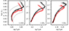 |
Fig. B.1. HRD showing stellar evolution tracks unseen by the CNF, and the sampling of these tracks by the CNF. The red colour indicates fCBM = 0.01, the black colour indicates fCBM = 0.02. In the left panel, tracks for 1.4 and 1.5 M⊙ (fCBM = 0.015, ω0 = 0.05) are shown in grey to illustrate the distance between two evolution tracks in the grid and the interpolation error of the CNF. |
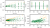 |
Fig. B.2. Discrepancy between the actual value and the recovered parameter for a set of validation data points (Δx = xactual − xrecovered). The green colour indicates values that are recovered within the 68%-confidence interval, the orange colour within twice this interval. |
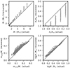 |
Fig. B.3. Actual value of the parameter in the mock data for Z = 0.0045 versus the recovered value when a metallicity of Z = 0.014 is assumed in the modelling. The solid black lines indicate the 1:1 line. |
All Tables
All Figures
|
Fig. 1. Pulsational characteristics of the sample. From top to bottom: amplitude of dominant frequency in the TESS light curve (in mmag), dominant frequency, and number of significant frequencies in the nominal TESS data. The bottom panel shows the number of stars above a given threshold on the classification probability Ppred from Hey & Aerts (2024). Vertical dashed lines indicate the used threshold in Ppred for the different samples. |
| In the text | |
|
Fig. 2. Hertzsprung-Russell diagrams showing the sample of g-mode pulsators with Ppred ≥ 0.5 (grey symbols with error bars). The evolutionary tracks show the extend of the grid of rotating stellar models, covering a mass range of [1.3, 9] M⊙, where the black (red) colour indicates ω0 = 0.05 (0.55), and the solid (dashed) line style fCBM = 0.005 (0.025). |
| In the text | |
|
Fig. 3. Kernel density estimations of the MLEs for the stellar mass (top-left), the fraction of initial hydrogen in the core (top-right), the fractional core mass (bottom-left), and the stellar radius (bottom-right), assuming Z = 0.0045. The different colours indicate different threshold on the classification probability from Hey & Aerts (2024) for the star to be considered a g-mode pulsator. The red line in the top-left panel corresponds to a Salpeter IMF with dN/dM ∝ M−2.35. |
| In the text | |
|
Fig. 4. Same as Fig. 3, but for Ppred ≥ 0.5 (in black) and the result of 1000 iterations of bootstrapping (in grey). The inset in the top-left panel shows a zoom-in around the mass range of γ Dor pulsators. |
| In the text | |
|
Fig. 5. Resulting p value from a one-sample Kolomogorov-Smirnov test between the inferred mass distribution of the sample of g-mode pulsators and a Salpeter IMF, as a function of the mass range tested. The upper mass is always 4 M⊙. The solid lines correspond to Z = 0.0045, the dashed lines correspond to Z = 0.014. The solid red line indicates a p value of 0.05 below which we reject the null hypothesis. |
| In the text | |
|
Fig. 6. Relation between the inferred stellar mass and the measured luminosity from Gaia of the stars in the sample. The solid red line indicates the fitted mass-luminosity relation, yielding log(L⋆/L⊙)=4.0623(6)log(M⋆/M⊙)+0.3468(2). The black triangles indicate bin averaged-values. Average uncertainties are indicated by the red data point. |
| In the text | |
|
Fig. 7. Relation between the inferred stellar mass and fractional convective core mass of the stars in the sample. The solid black (red) line indicates the maximum core mass possible during the main sequence for fCBM = 0.005 (0.025). The dashed lines show the maximum core mass at Xc/Xini = 0.4 (same colour coding). Average uncertainties are indicated by the red data point. |
| In the text | |
|
Fig. 8. Relation between the inferred stellar mass and the inferred stellar radius (from models) of the stars in the sample. The solid red line indicates a two-component linear fit to the data (see text). The black triangles indicate bin averaged-values. Average uncertainties are indicated by the red data point. |
| In the text | |
|
Fig. 9. Relation between the inferred fraction Xc/Xini and the convective core mass for stars M⋆ > 2 M⊙. The black triangles indicate the average per bin and standard deviation. Two models are shown for 2.4 M⊙ and ω0 = 0.05, where the mass is representative of the median stellar mass per bin as shown in the inset. The black colour corresponds to fCBM = 0.005, the red colour to fCBM = 0.025. |
| In the text | |
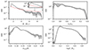 |
Fig. 10. Same as Fig. 4, but for Z = 0.014. |
| In the text | |
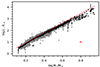 |
Fig. A.1. Same as Fig. 6, but for Z = 0.014. |
| In the text | |
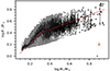 |
Fig. A.2. Same as Fig. 8, but for Z = 0.014. |
| In the text | |
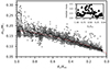 |
Fig. A.3. Same as Fig. 9, but for Z = 0.014. |
| In the text | |
|
Fig. B.1. HRD showing stellar evolution tracks unseen by the CNF, and the sampling of these tracks by the CNF. The red colour indicates fCBM = 0.01, the black colour indicates fCBM = 0.02. In the left panel, tracks for 1.4 and 1.5 M⊙ (fCBM = 0.015, ω0 = 0.05) are shown in grey to illustrate the distance between two evolution tracks in the grid and the interpolation error of the CNF. |
| In the text | |
|
Fig. B.2. Discrepancy between the actual value and the recovered parameter for a set of validation data points (Δx = xactual − xrecovered). The green colour indicates values that are recovered within the 68%-confidence interval, the orange colour within twice this interval. |
| In the text | |
|
Fig. B.3. Actual value of the parameter in the mock data for Z = 0.0045 versus the recovered value when a metallicity of Z = 0.014 is assumed in the modelling. The solid black lines indicate the 1:1 line. |
| In the text | |
Current usage metrics show cumulative count of Article Views (full-text article views including HTML views, PDF and ePub downloads, according to the available data) and Abstracts Views on Vision4Press platform.
Data correspond to usage on the plateform after 2015. The current usage metrics is available 48-96 hours after online publication and is updated daily on week days.
Initial download of the metrics may take a while.