| Issue |
A&A
Volume 685, May 2024
|
|
|---|---|---|
| Article Number | A21 | |
| Number of page(s) | 6 | |
| Section | Stellar structure and evolution | |
| DOI | https://doi.org/10.1051/0004-6361/202449213 | |
| Published online | 30 April 2024 | |
Probability distributions of initial rotation velocities and core-boundary mixing efficiencies of γ Doradus stars
1
IRAP, Université de Toulouse, CNRS, UPS, CNES, 14 Avenue Édouard Belin, 31400 Toulouse, France
e-mail: This email address is being protected from spambots. You need JavaScript enabled to view it.
2
Institute of Astronomy, KU Leuven, Celestijnenlaan 200D, 3001 Leuven, Belgium
3
Department of Astrophysics, IMAPP, Radboud University Nijmegen, PO Box 9010 6500 GL Nijmegen, The Netherlands
4
Max Planck Institute for Astronomy, Koenigstuhl 17, 69117 Heidelberg, Germany
5
I-BioStat, Universiteit Hasselt, Martelarenlaan 42, 3500 Hasselt, Belgium
6
I-BioStat, KU Leuven, Kapucijnenvoer 7, 3000 Leuven, Belgium
Received:
11
January
2024
Accepted:
7
February
2024
Abstract
Context. The theory of rotational and chemical evolution is incomplete, thereby limiting the accuracy of model-dependent stellar mass and age determinations. The γ Doradus (γ Dor) pulsators are excellent points of calibration for the current state-of-the-art stellar evolution models, as their gravity modes probe the physical conditions in the deep stellar interior. Yet, individual asteroseismic modelling of these stars is not always possible because of insufficient observed oscillation modes.
Aims. This paper presents a novel method to derive distributions of the stellar mass, age, core-boundary mixing efficiency, and initial rotation rates for γ Dor stars.
Methods. We computed a grid of rotating stellar evolution models covering the entire γ Dor instability strip. We then used the observed distributions of the luminosity, effective temperature, buoyancy travel time, and near-core rotation frequency of a sample of 539 stars to assign a statistical weight to each of our models. This weight is a measure of how likely the combination of a specific model is. We then computed weighted histograms to derive the most likely distributions of the fundamental stellar properties.
Results. We find that the rotation frequency at zero-age main sequence follows a normal distribution, peaking at around 25% of the critical Keplerian rotation frequency. The probability-density function for extent of the core-boundary mixing zone, given by a factor of fCBM times the local pressure scale height (assuming an exponentially decaying parameterisation), decreases linearly with increasing fCBM.
Conclusions. Converting the distribution of fractions of critical rotation at the zero-age main sequence to units of d−1, we find most F-type stars start the main sequence with a rotation frequency between 0.5 d−1 and 2 d−1. Regarding the core-boundary mixing efficiency, we find that it is generally weak in this mass regime.
Key words: asteroseismology / stars: evolution / stars: interiors / stars: oscillations / stars: rotation
© The Authors 2024
 Open Access article, published by EDP Sciences, under the terms of the Creative Commons Attribution License (https://creativecommons.org/licenses/by/4.0), which permits unrestricted use, distribution, and reproduction in any medium, provided the original work is properly cited.
This article is published in open access under the Subscribe to Open model. This email address is being protected from spambots. You need JavaScript enabled to view it. to support open access publication.
1. Introduction
The state-of-the-art stellar structure and evolution models that are the basis of many stellar-ageing methods lack a complete picture of chemical mixing. In the case of stars that maintain a convective core during the main-sequence phase, our ignorance regarding the efficiency of chemical mixing is often parameterised by a function for the core-boundary mixing (CBM; e.g. Zahn 1991; Freytag et al. 1996; Augustson & Mathis 2019) and a function for the mixing in the radiative envelope (e.g. Pedersen et al. 2021), both with at least one free parameter. The exact choice for these free parameters can result in age differences of about 40% by the end of the main sequence (Mombarg 2022), or up 15% between models with and without time-dependent, self-consistent convective penetration (Johnston et al. 2023). In addition, chemical mixing is induced by rotational shear (e.g. Zahn 1992), and therefore we require an accurate description for the transport of angular momentum. Yet, confrontations of predictions of angular momentum transport with asteroseismic measurements of the rotation velocities of stars have shown that the current physics is not adequate (Eggenberger et al. 2012; Marques et al. 2013; Cantiello et al. 2014; Aerts et al. 2019).
The class of γ Doradus (γ Dor) gravity-(g) mode pulsators (Kaye et al. 1999) has proven useful in constraining the near-core rotation (Van Reeth et al. 2016; Christophe et al. 2018; Li et al. 2019, 2020), the (radial) differential rotation (Van Reeth et al. 2018; Ouazzani et al. 2020; Saio et al. 2021), and the stellar mass and age (e.g. Mombarg et al. 2019, 2021; Mombarg 2023). As such, these constraints can be used to test the theory of angular momentum (Ouazzani et al. 2019; Moyano et al. 2023). In particular, Mombarg (2023) tested a diffusive approach for angular momentum transport on a set of slowly rotating γ Dor pulsators by combining their measured rotation frequencies from Li et al. (2019) with asteroseismic masses, ages, and CBM efficiencies using the method of Mombarg et al. (2021). When testing angular momentum transport, assumptions have to be made about the initial rotation. In the study of Ouazzani et al. (2019), the rotation frequency at the zero-age main sequence (ZAMS) is estimated from a stellar disc model with free parameters calibrated to cluster data, while in the studies of Moyano et al. (2023) and Mombarg (2023) the (uniform) rotation at the ZAMS is left as a free parameter. Mombarg (2023) concludes that the six slowly-rotating stars in his sample also had a slow rotation (less than 10% of the critical rotation frequency) to begin with. However, the distribution of rotation frequencies at the ZAMS for γ Dor pulsators or F-type stars is generally not well known, and this paper aims to improve on that. Similarly, the distribution of the efficiency of the CBM that needs to be added to obtain the core masses inferred by asteroseismic modelling is not well known (Johnston 2021; Pedersen 2022a). Individual measurements of the CBM efficiency have been made by modelling the observed mode frequencies of main-sequence g-mode pulsators (e.g. Johnston et al. 2019; Mombarg et al. 2021; Michielsen et al. 2019, 2023; Szewczuk et al. 2022) and of subgiants (e.g. Deheuvels & Michel 2011; Deheuvels et al. 2016; Noll et al. 2021). The first step (after frequency extraction) in the modelling of a g-mode pulsator is identifying the spherical degree (ℓ), azimuthal order (m), and radial order (n) of the excited pulsation frequencies. This is done by exploiting the relation that consecutive radial orders with the same (ℓ, m)-combination form a pattern when the difference in period between consecutive modes as plotted against the mode period itself (Tassoul 1980; Miglio et al. 2008; Bouabid et al. 2013). Once such a period-spacing pattern is identified, the near-core rotation frequency and buoyancy travel time (Π0, an asteroseismic quantity related to the g-mode cavity) can be measured, as first put into practice by Degroote et al. (2010).
The current largest sample of γ Dor pulsators with identified period-spacing patterns is that of Li et al. (2020), comprising 611 stars. In the case of single γ Dor stars, a precise measurement of the CBM efficiency requires both a sufficient number of identified radial orders and a precise constraint on the effective temperature. Apart from a sub-sample of 37 stars with spectroscopically derived effective temperatures already modelled by Mombarg et al. (2021), a large part of the sample of Li et al. (2020) does not allow for precise constraints on the CBM efficiency. However, as also shown by Garcia et al. (2022), measurements of the near-core rotation frequency and buoyancy travel time (Π0) can be made more easily.
The aim of this paper is to present a novel method to place constraints on the CBM efficiency and initial rotation velocity using the complete sample of γ Dor pulsators. This methodology is based on modelling the distributions of the observed luminosity, effective temperature, buoyancy travel time, and near-core rotation frequency of γ Dor pulsators. Relying on distributions instead of individual measurements makes this method less susceptible to individual uncertainties, as long as the sample size is sufficiently large.
2. Statistical methodology
In this paper, we make use of the largest sample of γ Dor to-date from Li et al. (2020), comprising 611 stars observed with the NASA Kepler mission (Borucki et al. 2010). We are interested in finding the distributions of the stellar mass, M⋆, the hydrogen-mass fraction in the core (proxy for age), Xc, the efficiency of CBM, fCBM (further discussed in Sects. 3 and 4), and the rotation velocity at zero-age main sequence (ZAMS) as a fraction of the Keplerian critical rotation frequency, ω0≡ (Ωsurf/Ωcrit)ZAMS. As observables, we have the distributions of the luminosity, L⋆, derived from the Gaia DR2 parallax (Murphy et al. 2019), of the effective temperature, Teff, from Mathur et al. (2017), of the buoyancy travel time, Π0, and of the near-core rotation frequency probed by the g modes, Ωcore. The buoyancy travel time is defined as
 (1)
(1)
and the near-core rotation frequency as
 (2)
(2)
Here, N is the Brunt–Väisälä frequency, Ω the local angular rotation velocity, and r the radial coordinate. Both integrals are evaluated over the g-mode cavity, which is defined as the region where the mode frequency in the corotating frame is smaller than N. Spectroscopically derived effective temperatures are available for only about 50 of the 611 stars (Gebruers et al. 2021). Therefore, we rely on the photometric ones.
To estimate the most likely values of the four fundamental parameters, given the distributions of the observed quantities and their precisions, we compute weighted histograms, for which we define a weight  as follows. First, let
  be a vector containing the observed quantities of star i ∈ [1, …, N]. We then compute a mean vector
  and variance-covariance matrix
  :
:
 (3)
(3)
 (4)
(4)
The weight of a model with observables  is then given by
 (5)
(5)
(see Johnson & Wichern 2002 for a basic introduction into multivariate data analysis). For each model  producing observables
  , the count towards a bin is weighted by
  . We normalised each of the components of
  and
and  by the corresponding maximum value in the observed distribution to ensure each of the four observables contributes equally to the value of
  . Furthermore, we take the same number of Xc variations per model, such that the distributions of all components of
  are uniformly sampled (see black dashed lines in Fig. 1).
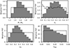 |
Fig. 1. Weighted probability density functions of stellar mass (top left), hydrogen-mass fraction in the core (top right), fraction of critical rotation at the ZAMS (bottom left), and CBM efficiency (bottom right). The black dashed lines show the occurrence of each value in the grid ( |

The sample of Li et al. (2020) contains stars for which there is no luminosity available or that have a measurement of Π0 larger than 6000 s and are thus more likely to be slowly pulsating B-type (SPB) stars (Waelkens 1991; Pedersen et al. 2021). Furthermore, any known binary system is also excluded. This constitutes 31 stars based on the absence of a luminosity measurement, 31 based on a too high value of Π0, and ten based on binarity. This leaves us with a final sample of 539 stars.
3. Stellar models
In order to compute the vectors  for a given set of model parameters
  , a grid of stellar models was computed with MESA (r23.05.1; Paxton et al. 2011, 2013, 2015, 2018, 2019; Jermyn et al. 2023). The three fundamental parameters that are varied are the mass, the surface rotation velocity at the ZAMS as a fraction of the critical rotation frequency, and the core-boundary mixing efficiency. For the latter, an exponentially decaying parameterisation of the chemical diffusion parameter was chosen following Freytag et al. (1996):
 (6)
(6)
Here, hP(rcore) is the pressure scale height at the radius of the convective core, and r0 is set to rcore − 0.005hP(rcore). The parameter fCBM is a free parameter determining the efficiency of the CBM. One of the aims of this paper is to find a distribution for this parameter, along with the mass, age, and initial rotation velocity.
Table 1 shows the range and step size for each of the four parameters in the grid, which contains ∼10 000 models (i.e. different combinations for  ). The chemical mixing in the radiative envelope is based on the work of Zahn (1992) using the MESA implementation of Mombarg et al. (2022). The chemical diffusion coefficient is determined by
 (7)
(7)
Ranges and step sizes of the different parameters varied in the MESA grid.
where K is the thermal diffusivity and η is a free parameter. As the actual local chemical diffusion coefficient, we took the largest one out of DCBM(r),Drot, or the one from convection. We set the parameter η to 1. As discussed in Mombarg et al. (2022), the shear profile dΩ/dr is scaled from a 2D ESTER model (Espinosa Lara & Rieutord 2013; Rieutord et al. 2016) that computes the differential rotation in a self-consistent manner. This way, a smooth profile of the Brunt–Väisälä frequency is ensured, which is necessary for computing asteroseismic quantities. We also included microscopic diffusion (gravitational settling and radiative levitation) for all elements with available monochromatic opacities from the OP Project (Seaton 2005) using the method outlined in Mombarg et al. (2022) and Jermyn et al. (2023). In doing so, we neglected the feedback of the change in the local mixture due to microscopic diffusion in the computation of the Rosseland mean opacity, which is calculated from the tables of the OP Project.
We assumed a fixed solar metallicity of 0.014 for our models, as spectroscopic studies of samples of Keplerγ Dor stars have shown that the average metallicity is close to the solar value (e.g. Van Reeth et al. 2015; Kahraman Aliçavuş et al. 2016; Gebruers et al. 2021). For the initial chemical composition of the models, (Xini, Yini, Zini), we assumed a galactic chemical enrichment rate of Yini = 0.244 + 1.226Zini (Verma et al. 2019), giving Yini = 0.261 and Xini = 0.725. For the relative metal fractions, we assumed the solar mixture according to Asplund et al. (2009).
For each model, we computed a non-rotating pre-main sequence model and relaxed this model to the desired rotation velocity at the ZAMS. The efficiency of angular momentum transport (given by the viscosity) is computed within the diffusive approach of MESA (see Heger et al. 2000 for the physical descriptions), which includes dynamical shear instability, secular shear instability, Eddington–Sweet, Solberg–Høiland instability, Goldreich–Schubert–Fricke instability, and a Spruit–Tayler dynamo.
4. Inferred distributions
For each model in the grid, we computed a weight  according to Eq. (5). Then, for M⋆, Xc, fCBM, and ω0, we plotted the weighted probability density distributions (PDFs). The top left panel of Fig. 1 shows the resulting distribution of the stellar mass, which is a skewed distribution around a mass of 1.5–1.6 M⊙. It should be noted that the γ Dor phenomenon only occurs during a certain part of a star’s main-sequence lifetime. Based on theoretical predictions for the γ Dor instability strip, stars with masses close to the edges of the grid (around 1.2 or 2 M⊙) will spend a smaller fraction of their main-sequence lifetime within the instability strip compared to stars around 1.6 M⊙. Therefore, we indeed expect such a skewed distribution distribution instead of recovering the initial-mass function. Yet, the fact that a non-negligible fraction of stars have a mass > 1.8 M⊙ suggests that the blue edge of the theoretically-predicted γ Dor instability strip (Dupret et al. 2005) should in reality be extended to higher effective temperatures.
The bottom-left panel of Fig. 1 shows the distribution of the rotation frequencies at the ZAMS as a fraction of the Keplerian critical rotation frequency (at ZAMS). We recovered a skewed distribution of the PDF that is centred around ω0 = 0.25. The study by Li et al. (2020) shows an excess of stars with very low near-core rotation frequencies (< 0.15 d−1) for which Mombarg (2023) concludes these stars were born as slow rotators (ω0 < 0.1). From the distribution of ω0 we recover here, no excess of slow rotators is observed. We also studied the distribution of the (uniform) rotation frequency at ZAMS when we do not scale it with the critical rotation frequency. The distribution is shown in Fig. 2. As can be seen from the dashed black line in this figure, a uniform distribution of the mass and ω0, does not give a uniform distribution in ΩZAMS.
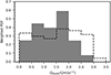 |
Fig. 2. Probability density function of uniform rotation rate at ZAMS in units of d−1. The black dashed line shows the distribution of the models in the grid, and the grey histogram shows the weighted distribution. |
Irrespective of the choice for the binning of the weighted PDF for ΩZAMS, we conclude that most γ Dor stars reach the ZAMS with a rotation frequency between 0.5 and 2 d−1 (5.8–23.2 μHz), although tails at lower and higher rotation frequency are populated as well. Mombarg et al. (2021) estimated the distribution of the initial rotation at the ZAMS of a sample of 37 γ Dor stars. Combining the present-day measured near-core rotation frequency (Van Reeth et al. 2016) with the asteroseismic mass and age, an estimate for the rotation at ZAMS can be made, assuming uniform rotation throughout the main sequence. When looking at the distribution of the initial rotation frequencies found by Mombarg et al. (2021), a peak around 2 d−1 is also seen. We find no stars with ΩZAMS/(2π)≳3 d−1. This corresponds to the upper limit of the measured near-core rotation frequencies of the γ Dor stars from Li et al. (2020) that were used in this paper (see also Fig. 6 in the summary plot by Aerts 2021).
Fritzewski et al. (2024a) performed modelling of the solar-metallicity young open cluster UBC 1 from TESS and Gaia space data and found an age between 150 and 300 Myr. This cluster is much younger than the Kepler field γ Dor stars we used to deduce the distributions. UBC 1 includes one γ Dor member with a near-core rotation frequency measurement, with a value of 0.544 ± 0.009 d−1, which is in agreement with our results for the distribution of rotation rates near the ZAMS. On the other hand, measurements of the near-core rotation frequency of γ Dor stars in the even younger open cluster NGC 2516 (102 ± 15 Myr, also solar metallicity) reveal eight of the 11 g-mode pulsators to have near-core rotation frequencies around 3 d−1, while the other three have values between 1 d−1 and about 2.2 d−1 (Li et al. 2024). At this estimated cluster age, these stars should be even closer to the ZAMS than the γ Dor member of UBC 1. The rotation rates for the majority of them occurs in the tail of our distribution in Fig. 2. Therefore, very young cluster γ Dor stars seem to occupy the full range of ZAMS rotation frequencies covered by the distribution we derived from the much older Kepler field stars in the galaxy and may have a less peaked distribution than the one in Fig. 2 given the possible selection bias for the youngest γ Dor pulsators in the Li et al. (2020) sample, as further discussed in Fritzewski et al. (2024b). Finally, with the physics of angular momentum transport used in this paper, we observe models reaching critical rotation during the main sequence, when ω0 ≳ 0.5.
The bottom right panel of Fig. 1 shows the distribution of the CBM parameter, fCBM (Eq. (6)). We observe a maximum probability density at the lower edge of the grid, fCBM = 0.005, and a probability density that decreases linearly with fCBM. We find that a value of 0.005 is about twice as likely as a value of 0.035. Thus, larger values are less likely, yet not negligible from a statistical point of view. Therefore, we can conclude that a universal value for fCBM is not reality, as also advocated by Johnston (2021). The study of Mombarg et al. (2021) presents individual measurements of fCBM (same physical prescription as we use here, apart from the prescription for the envelope mixing) for a sample of 37 γ Dor stars. For 30 stars in their sample, the value of fCBM could be constrained within the ranges of their grid. We show their distribution of fCBM in Fig. 3. Interestingly, the distribution of Mombarg et al. (2021) seems to also follow a linear decrease with the value of fCBM.
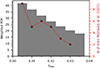 |
Fig. 3. Same probability density function as bottom right panel of Fig. 1 overplotted with the results of the individually measured fCBM values from Mombarg et al. (2021; red stars). |
5. Influence of input parameters
In this section, we quantify the contribution of each of the four observables in  to the final PDFs. As such, we repeat the methodology of Sect. 2, but omitting one of the observables at a time. From the resulting PDFs shown in Fig. 4, we can draw the following conclusions. Firstly, it is obvious that the distribution of ω0 is mostly determined by the present-day distribution of the near-core rotation frequencies and that the other fundamental stellar parameters are only mildly influenced. This is expected as there is no feedback of the rotation on the envelope mixing in our models. Secondly, omitting the luminosity results in a slightly higher PDF for more massive stars, which are expected to show γ Dor pulsations at the end of the main sequence, thus also increasing the probability for more evolved stars. Thirdly, the value of Π0 is sensitive to the core mass (e.g. Mombarg et al. 2019) and thus omitting this observable has a large impact on the PDF of fCBM. Moreover, since the value of Π0 drops off rapidly near the terminal-age main sequence (TAMS), including this observable eliminates the peak in stars near the TAMS, as shown in the top right panel of Fig. 4. Finally, we see that the effective temperature is an important parameter to break degeneracies of Π0 with respect to mass and age. The effective temperature has an even larger effect on the resulting PDF of fCBM compared to Π0. Increasing the extent of the CBM zone results in a higher effective temperature at the same luminosity. Therefore, without an effective temperature, models with a larger value for fCBM become equally likely, resulting in a flatter PDF.
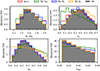 |
Fig. 4. Same as Fig. 1, but each time one of the observables in |

6. Conclusions
In this paper, we present a novel method to obtain the stellar mass, age, core-boundary mixing efficiency, and initial rotation frequency distributions of pulsating F-type (γ Dor) stars. We used the observed distributions of the luminosity, effective temperature, buoyancy travel time and near-core rotation frequency of a sample of 539 stars with high-precision estimates of these four variables taken from the Kepler asteroseismic γ Dor catalogue published by Li et al. (2020). We computed a grid of rotating (1D) stellar models for different masses, ages, core-boundary mixing efficiencies and initial rotation velocities at the ZAMS and assigned a statistical weight to each stellar model to obtain the probability density functions of these four fundamental stellar parameters. This method allows us to also include stars that are not suitable for asteroseismic modelling of the individual mode frequencies. The method is robust against individual measurement errors, as long as the sample is large enough to accurately sample average values and covariances of the observables.
The distributions presented in this paper can be used as priors for future modelling using a Bayensian framework or for population synthesis of pulsating F-type stars. We find skewed distributions of the probability density function for the mass, hydrogen-mass fraction in the core (Xc, proxy for age), and fraction of critical rotation at the ZAMS (ω0). These distributions peak around 1.6 M⊙, Xc = 0.4, and ω0 = 0.25. We find the probability distribution of the extent of the core-boundary mixing region (assuming an exponentially decaying function) to be linearly decreasing with increasing fCBM. The results on the initial rotation and core-boundary mixing presented in this paper are consistent with results from star-by-star modelling of the individual observed mode periods performed by Mombarg et al. (2021).
The method presented in this paper could also be applied to the SPB class of gravity mode pulsators. Currently, the sample size of SPB stars with measured Π0 values and near-core rotation frequencies is about a factor of ten smaller (see Pedersen 2022b, and references therein) compared to the γ Dor stars. Fortunately, this number is expected to increase from more extensive data sets being assembled by the NASA TESS mission (Ricker et al. 2015) and the upcoming ESA PLATO mission (Rauer et al. 2014).
Acknowledgments
The research leading to these results has received funding from the French Agence Nationale de la Recherche (ANR), under grant MASSIF (ANR-21-CE31-0018-02). The computational resources and services used in this work were provided by the VSC (Flemish Supercomputer Center), funded by the Research Foundation – Flanders (FWO) and the Flemish Government department EWI. C.A. acknowledges financial support from the KU Leuven Research Council (grant C16/18/005: PARADISE) and from the European Research Council (ERC) under the Horizon Europe programme (Synergy Grant agreement N°101071505: 4D-STAR). While partially funded by the European Union, views and opinions expressed are however those of the author(s) only and do not necessarily reflect those of the European Union or the European Research Council. Neither the European Union nor the granting authority can be held responsible for them. The authors are grateful to the anonymous referee for their feedback. This research made use of the numpy (Harris et al. 2020) and matplotlib (Hunter 2007) Python software packages.
References
- Aerts, C. 2021, Rev. Mod. Phys., 93, 015001 [Google Scholar]
- Aerts, C., Mathis, S., & Rogers, T. M. 2019, ARA&A, 57, 35 [Google Scholar]
- Asplund, M., Grevesse, N., Sauval, A. J., & Scott, P. 2009, ARA&A, 47, 481 [NASA ADS] [CrossRef] [Google Scholar]
- Augustson, K. C., & Mathis, S. 2019, ApJ, 874, 83 [Google Scholar]
- Borucki, W. J., Koch, D., Basri, G., et al. 2010, Science, 327, 977 [Google Scholar]
- Bouabid, M.-P., Dupret, M.-A., Salmon, S., et al. 2013, MNRAS, 429, 2500 [NASA ADS] [CrossRef] [Google Scholar]
- Cantiello, M., Mankovich, C., Bildsten, L., Christensen-Dalsgaard, J., & Paxton, B. 2014, ApJ, 788, 93 [Google Scholar]
- Christophe, S., Ballot, J., Ouazzani, R. M., Antoci, V., & Salmon, S. J. A. J. 2018, A&A, 618, A47 [NASA ADS] [CrossRef] [EDP Sciences] [Google Scholar]
- Degroote, P., Briquet, M., Auvergne, M., et al. 2010, A&A, 519, A38 [NASA ADS] [CrossRef] [EDP Sciences] [Google Scholar]
- Deheuvels, S., & Michel, E. 2011, A&A, 535, A91 [NASA ADS] [CrossRef] [EDP Sciences] [Google Scholar]
- Deheuvels, S., Brandão, I., Silva Aguirre, V., et al. 2016, A&A, 589, A93 [NASA ADS] [CrossRef] [EDP Sciences] [Google Scholar]
- Dupret, M.-A., Grigahcène, A., Garrido, R., et al. 2005, MNRAS, 360, 1143 [Google Scholar]
- Eggenberger, P., Montalbán, J., & Miglio, A. 2012, A&A, 544, L4 [NASA ADS] [CrossRef] [EDP Sciences] [Google Scholar]
- Espinosa Lara, F., & Rieutord, M. 2013, A&A, 552, A35 [NASA ADS] [CrossRef] [EDP Sciences] [Google Scholar]
- Freytag, B., Ludwig, H. G., & Steffen, M. 1996, A&A, 313, 497 [NASA ADS] [Google Scholar]
- Fritzewski, D. J., Van Reeth, T., Aerts, C., et al. 2024a, A&A, 681, A13 [NASA ADS] [CrossRef] [EDP Sciences] [Google Scholar]
- Fritzewski, D. J., Aerts, C., Mombarg, J. S. G., Gossage, S., & Van Reeth, T. 2024b, A&A, 684, A112 [NASA ADS] [CrossRef] [EDP Sciences] [Google Scholar]
- Garcia, S., Van Reeth, T., De Ridder, J., & Aerts, C. 2022, A&A, 668, A137 [NASA ADS] [CrossRef] [EDP Sciences] [Google Scholar]
- Gebruers, S., Straumit, I., Tkachenko, A., et al. 2021, A&A, 650, A151 [NASA ADS] [CrossRef] [EDP Sciences] [Google Scholar]
- Harris, C. R., Millman, K. J., van der Walt, S. J., et al. 2020, Nature, 585, 357 [NASA ADS] [CrossRef] [Google Scholar]
- Heger, A., Langer, N., & Woosley, S. E. 2000, ApJ, 528, 368 [NASA ADS] [CrossRef] [Google Scholar]
- Hunter, J. D. 2007, Comput. Sci. Eng., 9, 90 [NASA ADS] [CrossRef] [Google Scholar]
- Jermyn, A. S., Bauer, E. B., Schwab, J., et al. 2023, ApJS, 265, 15 [NASA ADS] [CrossRef] [Google Scholar]
- Johnson, R. A., & Wichern, D. W. 2002, Applied Multivariate Statistical Analysis (NJ: Prentice Hall Upper Saddle River) [Google Scholar]
- Johnston, C. 2021, A&A, 655, A29 [NASA ADS] [CrossRef] [EDP Sciences] [Google Scholar]
- Johnston, C., Tkachenko, A., Aerts, C., et al. 2019, MNRAS, 482, 1231 [Google Scholar]
- Johnston, C., Michielsen, M., Anders, E. H., et al. 2023, ApJ, accepted [arXiv:2312.08315] [Google Scholar]
- Kahraman Aliçavuş, F., Niemczura, E., De Cat, P., et al. 2016, MNRAS, 458, 2307 [CrossRef] [Google Scholar]
- Kaye, A. B., Handler, G., Krisciunas, K., Poretti, E., & Zerbi, F. M. 1999, PASP, 111, 840 [Google Scholar]
- Li, G., Bedding, T. R., Murphy, S. J., & Van Reeth, T. 2019, MNRAS, 482, 1757 [CrossRef] [Google Scholar]
- Li, G., Van Reeth, T., Bedding, T. R., et al. 2020, MNRAS, 491, 3586 [Google Scholar]
- Li, G., Aerts, C., Bedding, T. R., et al. 2024, A&A, in press, https://doi.org/10.1051/0004-6361/202348901 [Google Scholar]
- Marques, J. P., Goupil, M. J., Lebreton, Y., et al. 2013, A&A, 549, A74 [NASA ADS] [CrossRef] [EDP Sciences] [Google Scholar]
- Mathur, S., Huber, D., Batalha, N. M., et al. 2017, ApJS, 229, 30 [NASA ADS] [CrossRef] [Google Scholar]
- Michielsen, M., Pedersen, M. G., Augustson, K. C., Mathis, S., & Aerts, C. 2019, A&A, 628, A76 [NASA ADS] [CrossRef] [EDP Sciences] [Google Scholar]
- Michielsen, M., Van Reeth, T., Tkachenko, A., & Aerts, C. 2023, A&A, 679, A6 [NASA ADS] [CrossRef] [EDP Sciences] [Google Scholar]
- Miglio, A., Montalbán, J., Noels, A., & Eggenberger, P. 2008, MNRAS, 386, 1487 [Google Scholar]
- Mombarg, J. S. G. 2022, Ph.D. Thesis, KU Leuven, Belgium [Google Scholar]
- Mombarg, J. S. G. 2023, A&A, 677, A63 [NASA ADS] [CrossRef] [EDP Sciences] [Google Scholar]
- Mombarg, J. S. G., Van Reeth, T., Pedersen, M. G., et al. 2019, MNRAS, 485, 3248 [NASA ADS] [CrossRef] [Google Scholar]
- Mombarg, J. S. G., Van Reeth, T., & Aerts, C. 2021, A&A, 650, A58 [NASA ADS] [CrossRef] [EDP Sciences] [Google Scholar]
- Mombarg, J. S. G., Dotter, A., Rieutord, M., et al. 2022, ApJ, 925, 154 [NASA ADS] [CrossRef] [Google Scholar]
- Moyano, F. D., Eggenberger, P., Salmon, S. J. A. J., Mombarg, J. S. G., & Ekström, S. 2023, A&A, 677, A6 [NASA ADS] [CrossRef] [EDP Sciences] [Google Scholar]
- Murphy, S. J., Hey, D., Van Reeth, T., & Bedding, T. R. 2019, MNRAS, 485, 2380 [NASA ADS] [CrossRef] [Google Scholar]
- Noll, A., Deheuvels, S., & Ballot, J. 2021, A&A, 647, A187 [EDP Sciences] [Google Scholar]
- Ouazzani, R. M., Marques, J. P., Goupil, M. J., et al. 2019, A&A, 626, A121 [NASA ADS] [CrossRef] [EDP Sciences] [Google Scholar]
- Ouazzani, R. M., Lignières, F., Dupret, M. A., et al. 2020, A&A, 640, A49 [NASA ADS] [CrossRef] [EDP Sciences] [Google Scholar]
- Paxton, B., Bildsten, L., Dotter, A., et al. 2011, ApJS, 192, 3 [Google Scholar]
- Paxton, B., Cantiello, M., Arras, P., et al. 2013, ApJS, 208, 4 [Google Scholar]
- Paxton, B., Marchant, P., Schwab, J., et al. 2015, ApJS, 220, 15 [Google Scholar]
- Paxton, B., Schwab, J., Bauer, E. B., et al. 2018, ApJS, 234, 34 [NASA ADS] [CrossRef] [Google Scholar]
- Paxton, B., Smolec, R., Schwab, J., et al. 2019, ApJS, 243, 10 [Google Scholar]
- Pedersen, M. G. 2022a, ApJ, 930, 94 [NASA ADS] [CrossRef] [Google Scholar]
- Pedersen, M. G. 2022b, ApJ, 940, 49 [NASA ADS] [CrossRef] [Google Scholar]
- Pedersen, M. G., Aerts, C., Pápics, P. I., et al. 2021, Nat. Astron., 5, 715 [NASA ADS] [CrossRef] [Google Scholar]
- Rauer, H., Catala, C., Aerts, C., et al. 2014, Exp. Astron., 38, 249 [Google Scholar]
- Ricker, G. R., Winn, J. N., Vanderspek, R., et al. 2015, J. Astron. Telesc. Instrum. Syst., 1, 014003 [Google Scholar]
- Rieutord, M., Espinosa Lara, F., & Putigny, B. 2016, J. Comput. Phys., 318, 277 [NASA ADS] [CrossRef] [Google Scholar]
- Saio, H., Takata, M., Lee, U., Li, G., & Van Reeth, T. 2021, MNRAS, 502, 5856 [Google Scholar]
- Seaton, M. J. 2005, MNRAS, 362, L1 [Google Scholar]
- Szewczuk, W., Walczak, P., Daszyńska-Daszkiewicz, J., & Moździerski, D. 2022, MNRAS, 511, 1529 [NASA ADS] [CrossRef] [Google Scholar]
- Tassoul, M. 1980, ApJS, 43, 469 [Google Scholar]
- Van Reeth, T., Tkachenko, A., Aerts, C., et al. 2015, ApJS, 218, 27 [Google Scholar]
- Van Reeth, T., Tkachenko, A., & Aerts, C. 2016, A&A, 593, A120 [NASA ADS] [CrossRef] [EDP Sciences] [Google Scholar]
- Van Reeth, T., Mombarg, J. S. G., Mathis, S., et al. 2018, A&A, 618, A24 [NASA ADS] [EDP Sciences] [Google Scholar]
- Verma, K., Raodeo, K., Basu, S., et al. 2019, MNRAS, 483, 4678 [Google Scholar]
- Waelkens, C. 1991, A&A, 246, 453 [NASA ADS] [Google Scholar]
- Zahn, J. P. 1991, A&A, 252, 179 [Google Scholar]
- Zahn, J. P. 1992, A&A, 265, 115 [NASA ADS] [Google Scholar]
All Tables
All Figures
|
Fig. 1. Weighted probability density functions of stellar mass (top left), hydrogen-mass fraction in the core (top right), fraction of critical rotation at the ZAMS (bottom left), and CBM efficiency (bottom right). The black dashed lines show the occurrence of each value in the grid ( |
| In the text | |
|
Fig. 2. Probability density function of uniform rotation rate at ZAMS in units of d−1. The black dashed line shows the distribution of the models in the grid, and the grey histogram shows the weighted distribution. |
| In the text | |
|
Fig. 3. Same probability density function as bottom right panel of Fig. 1 overplotted with the results of the individually measured fCBM values from Mombarg et al. (2021; red stars). |
| In the text | |
|
Fig. 4. Same as Fig. 1, but each time one of the observables in |
| In the text | |
Current usage metrics show cumulative count of Article Views (full-text article views including HTML views, PDF and ePub downloads, according to the available data) and Abstracts Views on Vision4Press platform.
Data correspond to usage on the plateform after 2015. The current usage metrics is available 48-96 hours after online publication and is updated daily on week days.
Initial download of the metrics may take a while.