| Issue |
A&A
Volume 695, March 2025
|
|
|---|---|---|
| Article Number | A214 | |
| Number of page(s) | 16 | |
| Section | Stellar structure and evolution | |
| DOI | https://doi.org/10.1051/0004-6361/202452691 | |
| Published online | 24 March 2025 | |
Evolution of the near-core rotation frequency of 2497 intermediate-mass stars from their dominant gravito-inertial mode
1
Institute of Astronomy, KU Leuven, Celestijnenlaan 200D, B-3001 Leuven, Belgium
2
Department of Astrophysics, IMAPP, Radboud University Nijmegen, PO Box 9010 6500 GL Nijmegen, The Netherlands
3
Max Planck Institute for Astronomy, Königstuhl 17, 69117 Heidelberg, Germany
4
IRAP, Université de Toulouse, CNRS, UPS, CNES, 14 Avenue Édouard Belin, F-31400 Toulouse, France
5
Université Paris-Saclay, Université de Paris, Sorbonne Paris Cité, CEA, CNRS, AIM, 91191 Gif-sur-Yvette, France
6
Institute for Astronomy, University of Hawai’i, Honolulu, HI 96822, USA
⋆ Corresponding author; conny.aerts@kuleuven.be
Received:
21
October
2024
Accepted:
16
February
2025
Context. The sparsely sampled time-series photometry from Gaia Data Release 3 (DR3) led to the discovery of more than 100 000 main-sequence non-radial pulsators. The majority of these were further scrutinised by uninterrupted high-cadence space photometry assembled by the Transiting Exoplanet Survey Satellite (TESS).
Aims. We combined Gaia DR3 and TESS photometric light curves to estimate the internal physical properties of 2497 gravity-mode pulsators. We performed asteroseismic analyses with two major aims: (1) to measure the near-core rotation frequency and its evolution during the main sequence and (2) to estimate the mass, radius, evolutionary stage, and convective core mass from stellar modelling.
Methods. We relied on asteroseismic properties of Kepler γ Doradus and slowly pulsating B stars to derive the cyclic near-core rotation frequency, frot, of the Gaia-discovered pulsators from their dominant prograde dipole gravito-inertial pulsation mode. Further, we investigated the impact of adding frot as an extra asteroseismic observable apart from the luminosity and effective temperature on the outcome of grid-based modelling from rotating stellar models.
Results. We offer a recipe based on linear regression to deduce frot from the dominant gravito-inertial mode frequency. It is applicable to prograde dipole modes with an amplitude above 4 mmag and occurring in the sub-inertial regime. By applying it to 2497 pulsators with such a mode, we have increased the sample of intermediate-mass dwarfs with such an asteroseismic observable by a factor of four. We used the estimate of frot to deduce spin parameters between two and six, while the sample’s near-core rotation rates range from 0.7% to 25% of the critical Keplerian rate. We used frot, along with the Gaia effective temperature and luminosity to deduce the (convective core) mass, radius, and evolutionary stage from grid modelling based on rotating stellar models. We derived a decline of frot with a factor of two during the main-sequence evolution for this population of field stars, which covers a mass range from 1.3 M⊙ to 7 M⊙. We found observational evidence for an increase in the radial order of excited gravity modes as the stars evolve. For 969 pulsators, we derived an upper limit of the radial differential rotation between the convective core boundary and the surface from Gaia’s vbroad measurement and found values up to 5.4.
Conclusions. Our recipe to deduce the near-core rotation frequency from the dominant prograde dipole gravito-inertial mode detected in the independent Gaia and TESS light curves is easy to use, facilitates applications to large samples of pulsators, and allows to map their angular momentum and evolutionary stage in the Milky Way.
Key words: asteroseismology / waves / stars: evolution / stars: interiors / stars: oscillations / stars: rotation
© The Authors 2025
 Open Access article, published by EDP Sciences, under the terms of the Creative Commons Attribution License (https://creativecommons.org/licenses/by/4.0), which permits unrestricted use, distribution, and reproduction in any medium, provided the original work is properly cited.
This article is published in open access under the Subscribe to Open model. Subscribe to A&A to support open access publication.
1. Introduction
The internal rotation of stars continues to be one of the major uncertain ingredients in the theory of stellar evolution (Maeder 2009). Modelling of the dominant transport processes happening in the interiors of stars relies on poorly calibrated expressions involving the gradient of the angular rotation profile. To compute this gradient throughout the evolution of the star, the so-called shellular approximation introduced by Zahn (1992) is often adopted. Relying on this formulation, the profile of dΩ(r)/dr is used to evaluate the element and angular momentum processes in the stellar interior (e.g. Chaboyer & Zahn 1992; Heger et al. 2000; Maeder & Meynet 2000).
Over the past decade, asteroseismology (Aerts et al. 2010) has been a game changer in the study of stellar rotation. Progress on the internal rotation of stars has relied on the detection and interpretation of non-radial oscillation modes probing the deepest layers of stars. Dupret et al. (2009) provided theoretical predictions on the capacity of dipole mixed modes to probe the central regions of evolved low-mass stars, while Miglio et al. (2008) and Bouabid et al. (2013) described the properties of gravity and gravito-inertial modes in young intermediate-mass dwarfs. These theoretical studies have been turned into practical tools thanks to space asteroseismology (Hekker & Christensen-Dalsgaard 2017; García & Ballot 2019; Córsico et al. 2019; Aerts 2021; Kurtz 2022, for recent overviews).
Accurate values of the angular core or near-core rotation frequencies for thousands of stars have been deduced. This was achieved from dipole mixed modes in subgiants and red giants (measuring the core value of the rotation, Ωcore, see Beck et al. 2011, 2012; Bedding et al. 2011; Deheuvels et al. 2012; Mosser et al. 2012, 2014, 2015; Gehan et al. 2018) and from dipole gravity or gravito-inertial modes in dwarfs (measuring the near-core value, Ωnear − core, just outside the convective core, see Degroote et al. 2010; Pápics et al. 2012, 2014; Kurtz et al. 2014; Saio et al. 2015; Van Reeth et al. 2015a, 2016; Ouazzani et al. 2017; Pápics et al. 2017; Saio et al. 2018). The diagnostic observables used to deduce the measurements of the internal rotation can be rotationally split multiplets, or period spacing patterns of mixed modes or gravity modes affected by the Coriolis acceleration (see Aerts et al. 2019, for a review of the methodologies). From the stars that also have a measurement of the angular envelope rotation frequency (Ωenv), it was further established that strong (near-)core to envelope coupling occurs, keeping the level of differential rotation (Ω(near − )core/Ωenv) modest during the two longest phases of stellar evolution (Deheuvels et al. 2015; Triana et al. 2015; Van Reeth et al. 2018; Li et al. 2020; Ouazzani et al. 2020; Saio et al. 2021; Li et al. 2024). Further, it was established that the core rotation at the time of central helium exhaustion is in agreement with the rotation of white dwarfs (Hermes et al. 2017; Aerts et al. 2019). Moreover, Ω(near − )core/Ωenv increases strongly during hydrogen shell burning, reaching values of up to 20 (Deheuvels et al. 2014; Di Mauro et al. 2016; Triana et al. 2017; Deheuvels et al. 2020; Li et al. 2024).
Thanks to asteroseismology, our understanding of how angular momentum transport and angular momentum loss slow down the (core) rotation after exhaustion of the central hydrogen has improved dramatically (Fuller et al. 2019; Eggenberger et al. 2019a,b; Moyano et al. 2023a). These novel transport theories comply with the asteroseismic measurements of the internal rotation for thousands of evolved stars of low and intermediate mass. For the longest phase of stellar evolution, however, less than 100 dwarfs have both their Ωnear − core and Ωenv, or Ωnear − core and Ωsurf measured, where Ωsurf is the angular rotation frequency at the stellar surface (Li et al. 2020; Pedersen et al. 2021; Pedersen 2022a). Stars with these observables available cover the mass range of [1.3, 9] M⊙ and span a broad interval of measured near-core rotation rates (up to about 30 μHz, Aerts 2021). As a consequence, our understanding of angular momentum transport during core hydrogen burning is still limited, despite progress over the past five years (Fuller et al. 2019; Eggenberger et al. 2022; Bétrisey et al. 2023; Moyano et al. 2023b, 2024).
Here, our aim is to enlarge the sample of dwarfs with an estimate of the near-core rotation frequency and to study how it evolves in time during the main-sequence phase. We wish to deduce dΩ/dt in the transition zone from the convective core to the radiative envelope as stars evolve from the zero-age main sequence (ZAMS) to the terminal-age main sequence (TAMS). We achieve this by relying on a sample of thousands of new gravity-mode pulsators discovered from Data Release 3 (DR3) of the Gaia space mission (Gaia Collaboration 2023; Aerts et al. 2023). Hey & Aerts (2024) confirmed the pulsational nature of these stars on the basis of independently assembled light curves from the Transiting Exoplanet Survey Satellite (TESS). The sample of gravity-mode pulsators with both Gaia DR3 and TESS data in the public domain is 23 times larger than the Kepler sample of dwarfs with measurements of Ωnear − core (Mombarg et al. 2024a).
We worked towards our goal by relying on two well-established properties of main-sequence gravity-mode pulsators deduced from Kepler space-based photometry: (1) The majority of such pulsators reveal dominant prograde dipole modes (Van Reeth et al. 2016; Li et al. 2020); (2) the dominant mode in their amplitude spectra reveals a clear shift towards higher frequency according to their near-core rotation rate (Pápics et al. 2017; Aerts & Tkachenko 2024). In this work, we bring these two properties together and come up with a regression formula for the near-core rotation frequency from a measurement of the dominant oscillation frequency of the Kepler gravity-mode pulsators (Sect. 2). We apply our recipe to the new sample of confirmed gravity-mode pulsators discovered from Gaia and validated by TESS (Sect. 3). We perform grid modelling based on the near-core rotation frequency and the Gaia effective temperature and luminosity as non-seismic observables and compare the outcome with published evolutionary grid modelling without an asteroseismic estimate of Ωnear − core (Sect. 4). We end with conclusions and the prospect of deriving an asteroseismic measurement of the near-core rotation frequency for millions of dwarfs across the Milky Way from future combined Gaia DR4 and TESS data (Sect. 5).
2. A recipe for the near-core rotation frequency from a prograde dipole gravito-inertial mode
Gaia DR3 led to the discovery of more than 100 000 new candidate (non-)radial pulsators. Their dominant frequency have an amplitude above about 4 mmag (Gaia Collaboration 2023). Among the new non-radial pulsators, Aerts et al. (2023) selected those with an amplitude below 35 mmag and dominant frequency in the range [0.7, 3.2] d−1. These two extra criteria were found to be effective in selecting the γ Doradus (γ Dor) and slowly pulsating B (SPB) star candidates among the overall sample presented by Gaia Collaboration (2023). The global stellar parameters of these 15 062 candidate gravity-mode pulsators were found to be in good agreement with those of confirmed and well-studied Kepler pulsators of these two kinds (Aerts et al. 2023).
Hey & Aerts (2024) revisited the sample of more than 100 000 candidate main-sequence pulsators classified by Gaia Collaboration (2023). They extracted light curves for almost 60 000 of them from TESS Full Frame Images (FFIs) in the public domain. These densely sampled TESS light curves allowed them to confirm the dominant frequency found in the sparsely sampled Gaia DR3 time-series photometry for the majority of them. Hey & Aerts (2024) then reclassified the pulsators with a TESS FFI light curve. They came up with a cleaner sub-sample of gravity-mode pulsators among the multiperiodic variables, as improvement with respect to the Aerts et al. (2023) study.
Here, we consider a sub-sample of 15 692 pulsators classified by Hey & Aerts (2024) with a probability above 50% to be a γ Dor or SPB star or a hybrid pressure/gravity-mode pulsator. Mombarg et al. (2024a) determined the mass, radius, and evolutionary stage of these 15 692 pulsators from evolutionary grid modelling. This was done by matching the stars’ Gaia DR3 effective temperature and luminosity with those predicted from a grid of rotating stellar models calibrated by asteroseismology of Kepler gravity-mode pulsators, covering the mass range from 1.3 M⊙ to 9 M⊙.
For our study, we rely on the dominant pulsation mode of these 15 692 stars found consistently in the Gaia and TESS light curves to assess their cyclic near-core rotation frequency, denoted here for simplicity as frot ≡ Ωnear − core/2π. In order to achieve this, we first recall some general properties of well-studied Kepler gravity-mode pulsators.
2.1. Basic properties of gravito-inertial modes in dwarfs
Main-sequence pulsators of γ Dor or SPB type exhibit low-frequency gravity modes of high radial-order, n, excited by either the flux blocking mechanism or the κ mechanism (Pamyatnykh 1999; Guzik et al. 2000; Bouabid et al. 2013; Xiong et al. 2016; Szewczuk & Daszyńska-Daszkiewicz 2017). The majority of these pulsators experience moderate to fast rotation, which brings the oscillation modes into the sub-inertial regime, where both buoyancy and the Coriolis force act together as restoring forces (Aerts et al. 2019; Aerts & Tkachenko 2024). Such modes are called gravito-inertial modes, while modes in slow rotators restored by buoyancy alone are pure gravity modes.
In the asymptotic frequency limit, where the pulsation frequency in the co-rotating frame, fco, is much smaller than the Brunt-Väisälä frequency, N, and in the ‘Traditional Approximation of Rotation’ (TAR; e.g. Lee & Saio 1987; Townsend 2003), we have
where λkmν is the eigenvalue of the Laplace tidal equation for a mode labelled as (k, m) having spin parameter ν = 2frot/fco, αg is a phase term dependent on the boundaries of the pulsation mode cavity denoted by the positions r1 and r2, and the buoyancy radius is
For non-rotating stars, gravity modes are labelled by indices (l, m, n), where l and |m|≤l denote the degree and azimuthal order of the spherical harmonic Ylm describing the displacement vector of the mode. In this work, we define prograde and retrograde modes as having m > 0 and m < 0, respectively, while zonal modes have m = 0. In order to encompass a single mode classification procedure for rotating pulsators, Lee & Saio (1997) defined a suitable labelling scheme based on one unique integer index k because l is not suitable to capture all mode families. The value of k is able to represent all families of solutions to the Laplace tidal equation, which describes the oscillations when the vertical component of the Coriolis acceleration is taken into account, but not the horizontal component. In this labelling scheme, zero or positive values of k correspond to modes having a counterpart of the harmonic degree l = |m|+k in the limit of no rotation. On the other hand, negative k values stand for retrograde modes that do not have any counterpart in the non-rotating case (see also Townsend 2003, for more details on mode classification schemes in rotating pulsators). Our study is focused on stars with k ≥ 0 modes. In particular, zonal dipole gravity modes are labelled as (k, m) = (1, 0), tesseral quadrupole retrograde gravity modes have (k, m) = (1, −1), while prograde sectoral dipole gravity or gravito-inertial modes have (k, m) = (0, 1), all of which occur in Fig. 1 discussed below.
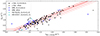 |
Fig. 1. Near-core rotation frequency frot plotted as a function of dominant mode frequency for Kepler gravity-mode pulsators having an observed amplitude above 4 mmag (fdom, ≥ 4 mmag) from the samples of Li et al. (2020) and Pedersen et al. (2021). Stars are drawn as γ Dor pulsator if they have Teff < 8500 K and Π0 < 0.7 d and as SPB star otherwise. When invisible, the error bars are smaller than the symbol sizes. The linear relation (red line) given by Eq. (4) was computed for the 105 stars having a dominant (k, m) = (0, 1) mode with observed frequency above 0.35 d−1 and with ν > 1 (full symbols). The shaded area shows the 1-σ uncertainty region for this relation. The two pulsators indicated in cyan come from short CoRoT light curves (Degroote et al. 2010; Pápics et al. 2012). As the other open symbols, they were not used in the regression. The dashed (dotted) lines mark the 1-σ confidence interval for frot derived from the residuals with respect to the red line, excluding (including) stars with modes having (k, m)≠(0, 1) or ν < 1. |
The condition that the mode frequencies must be well below N is fulfilled for γ Dor and SPB stars, as shown by Aerts et al. (2021, see their Fig. 1). Moreover, Aerts et al. (2017, 2021), and Pedersen (2022a) deduced the spin parameters of the identified modes of γ Dor and SPB pulsators and found ν ≥ 1 for almost all modes in the γ Dor stars and for the majority of them in SPB stars, justifying the use of the TAR in general terms for such pulsators (see Mathis et al. 2013, for extensive discussions on the TAR criteria).
In the limit of high radial order n ≫ 1 (corresponding to the limit of low frequencies), gravity or gravito-inertial modes of the same (k, m) and consecutive radial order n obey a regular pattern. This is predicted theoretically (Miglio et al. 2008; Bouabid et al. 2013; Van Reeth et al. 2015b; Ouazzani et al. 2017) and observed in photometry of single and binary pulsators assembled with the Convection, Rotation, and exoplanetary Transits (CoRoT), Kepler or TESS space telescopes (e.g. Degroote et al. 2010; Pápics et al. 2012, 2014; Kurtz et al. 2014; Saio et al. 2015; Van Reeth et al. 2015a; Keen et al. 2015; Pápics et al. 2017; Szewczuk & Daszyńska-Daszkiewicz 2018; Sekaran et al. 2020; Wu et al. 2020; Li et al. 2020; Szewczuk et al. 2021; Pedersen et al. 2021; Garcia et al. 2022; Kemp et al. 2024). These publications revealed the regular mode patterns detected in the space photometry to allow for mode identification. For the γ Dor stars, most of the observed modes identified as (k, m) = (0, 1) in these publications have radial order n ∈ [10, 100] (Li et al. 2020), while SPB stars typically have (k, m) = (0, 1) modes with n ∈ [10, 50] excited (Szewczuk & Daszyńska-Daszkiewicz 2017).
As elaborated by Aerts & Tkachenko (2024), the Coriolis force is more important than the the centrifugal force in the calculation of the modes for γ Dor and SPB stars. This is due to the mode energy being dominated by the region adjacent to the convective core, where the rotational deformation due to the centrifugal force is modest (Mathis & Prat 2019; Henneco et al. 2021; Dhouib et al. 2021a,b). Moreover, the horizontal components of the displacement vector of the modes are typically an order of magnitude larger than the vertical ones (De Cat & Aerts 2002). All of these properties together imply that the TAR is well justified, unless the stars rotate close to their critical rate. We discuss and evaluate this latter condition in Sect. 4.
2.2. Identification of the dominant mode of the Kepler gravity-mode pulsators
The combined Kepler gravity-mode pulsator samples analysed by Li et al. (2020), Pedersen et al. (2021), and Pedersen (2022b) reveal period-spacing patterns of prograde dipole modes for 610 of the 634 stars in the combined sample (96.2%). For 428 of these, that is 67.5% of the sample, the dominant mode was part of the detected pattern. When only stars with dominant pulsation amplitudes larger than 4 mmag are considered among these Kepler pulsators, which is the amplitude detection threshold for the discovery of the Gaia DR3 gravity-mode pulsators, this fraction increases to 84.7%.
Hence, in the remainder of this work we rely on the fact that the large majority among the dominant frequencies of well-characterised Kepler γ Dor and SPB stars correspond to a mode with (k, m) = (0, 1). While doing so, we keep in mind that about 15% of the dominant frequencies may belong to a mode with another identification of (k, m).
2.3. A regression formula for the internal rotation frequency
In the case of modes with k = 0 in moderate- to fast-rotating stars, that is, with ν ≫ 1, theory predicts that λkmν ≈ m2 (e.g. Townsend 2003). This leads to a quasi-linear relation between the observed cyclic gravity-mode frequencies fnkm and the near-core rotation frequency frot:
which has also been found observationally (e.g. Van Reeth et al. 2016; Pápics et al. 2017; Li et al. 2020; Audenaert & Tkachenko 2022). Here, we wish to exploit this relationship in the context of the newly discovered Gaia gravity-mode pulsators, whose observed dominant cyclic mode frequencies, fdom, are consistent in the DR3 and TESS data and which have amplitudes above 4 mmag. An earlier similar idea was put forward by Sepulveda et al. (2022, 2023) in the context of the exoplanet host stars 51 Eridani and HR 8799, which are both γ Dor pulsators. These authors considered an averaged frequency value among the dominant modes to infer the near-core rotation frequency in an empirical way by considering the sample of Li et al. (2020), without relying on the theory-based Eq. (3) as we do here.
To quantify the observational relation between frot and fdom we fitted a linear model to the Kepler results found for the homogeneously studied samples of γ Dor and SPB pulsators from Li et al. (2020) and Pedersen et al. (2021). In light of the application to the Gaia discovered gravity-mode pulsators, we only selected the Kepler pulsators with dominant pulsation amplitude above 4 mmag and identified as (k, m) = (0, 1), that is only stars with a dominant dipole prograde mode. Moreover, we demanded their dominant mode to occur in the sub-inertial regime, where ν > 1. In this way, we found the following regression fit based on the 100 γ Dor stars and five SPB stars with their dominant prograde dipole mode in the sub-inertial regime, having an observed amplitude above 4 mmag, and having been subjected to asteroseismic modelling from Kepler:

where all of frot, fdom, and 1/Π0 are expressed in d−1. This fit is illustrated by the full red line in Fig. 1. The strong correlation between frot and fdom is reflected by the Pearson correlation coefficient, which has a value of 0.942.
We applied a bootstrap analysis on the residuals of the fit in Eq. (4) and found that the estimated rotation frequency values have uncertainties σ− and σ+ of −0.164 d−1 and +0.123 d−1, respectively. The results for this confidence interval are graphically depicted in Fig. 2 by the dashed lines. If we also took into account the residuals with respect to the regression line for the ∼20% sample stars that have pulsations with other geometries (k, m)≠(0, 1) or in the super-inertial regime (ν < 1), we found uncertainties σ− and σ+ of −0.302 d−1 and +0.186 d−1, respectively. This confidence interval is delineated by the dotted lines in Figs. 1 and 2.
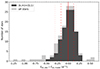 |
Fig. 2. Residuals from the linear fit described by Eq. (4) for the selected Kepler pulsators used in Fig. 1. The distribution of modes with (k, m) = (0, 1), ν > 1, and observed frequency above 0.35 d−1 is shown in dark grey, wile the distribution of all dominant modes with amplitude ≥4 mmag is shown in light grey. The full, dashed, and dotted lines indicate the same relation and confidence intervals as those in Fig. 1. |
For illustrative purposes, we also plot the two gravity-mode pulsators having an identified dominant mode from their 5-months-long light curve assembled by the CoRoT space telescope in Fig. 1. Even if their frequency precision is lower than the one deduced from 4-year duration Kepler light curves, they still occur in the vicinity of the Kepler pulsators with (k, m)≠(0, 1) modes. None of these stars (with open symbols) were used in the construction of the regression formula in Eq. (4).
2.4. The scaled buoyancy radius
For the observed dominant prograde dipole modes in the Kepler sample, we used Eq. (1) to derive Π0(n + αg), where we used the mode frequencies and the determined rotation frequencies frot as input. The results of this analysis are shown in Fig. 3. Here, the derived 1-σ confidence intervals were propagated from the confidence intervals of frot, derived using stratified residual bootstrapping (Davison & Hinkley 1997). The relative scatter of the Π0(n + αg) values is larger than of the frot values, as reflected by a lower Pearson correlation coefficient of 0.542.
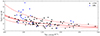 |
Fig. 3. The quantity Π0(n + αg) plotted as a function of the dominant prograde dipole gravity-mode frequency with amplitude above 4 mmag (fdom, ≥ 4 mmag) for 105 γ Dor and SPB stars from Li et al. (2020) and Pedersen et al. (2021). The symbols have the same meaning as in Fig. 1. The relation given by Eq. (3) is shown by the red line, while the shaded area shows the 1-σ uncertainty region. The dashed lines mark the 1-σ confidence region, propagated forward from the confidence regions of the frot values. |
While most Kepler sample stars are in agreement with the confidence regions, a few outliers with measured mode frequencies between 1 and 1.2 d−1 occur. These stars from Li et al. (2020) are SPB stars based on their Teff and our definition. They have anomalously high Π0 values, which may result from an overestimated frot value propagating into the derived high Π0(n + αg) values above 4.5 d.
3. Application to a Gaia sample
Hey & Aerts (2024, their Fig. 6) found a distinct ridge in the stacked amplitude periodograms of the gravity-mode pulsators, characteristic for prograde dipole modes as also found for the Kepler γ Dor pulsators by Li et al. (2020). Among the 15 692 Gaia DR3 gravity-mode pulsators modelled by Mombarg et al. (2024a), we defined a sub-sample with the aim to select a maximum number of stars with a high probability of having a dominant prograde dipole mode in the TESS FFI light curve.
We required that (i) the amplitudes and frequencies of the dominant pulsations in the Gaia DR3 light curves are ≥4 mmag and ≤3.2 d−1, respectively (Aerts et al. 2023), (ii) they were classified by Hey & Aerts (2024) as γ Dor or SPB star or else as hybrid gravity/pressure mode pulsator, in all of these three cases with a probability above 50%, (iii) the dominant frequencies measured from the Gaia and TESS data differ less than 0.1 d−1 (Hey & Aerts 2024), (iv) log(L/L⊙) ≥ 0, and (v) GGaia ≤ 13 mag. These stringent constraints delivered a sub-sample of 2497 pulsators among those with parameters from evolutionary modelling by Mombarg et al. (2024a), notably their mass M⋆, convective core mass mcc, radius R⋆, and evolutionary stage defined as the ratio of the hydrogen mass fraction remaining in the convective core compared to the initial value at birth, Xc/Xini.
Following Hey & Aerts (2024), Fig. 4 shows the stacked periodograms of these 2497 gravity-mode pulsators based on their TESS FFI light curves. A prominent ridge occurs, very similar to the one found for stars with dominant identified (k, m) = (0, 1) modes from Kepler light curves by Li et al. (2020). This lends support to our assumption that these Gaia gravity-mode pulsators have a dominant prograde dipole gravito-inertial mode. In the remainder of this work we reasonably assume that all the 2497 stars in our current sub-sample with periodogram shown in Fig. 4 fulfil the mode identification (k, m) = (0, 1).
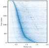 |
Fig. 4. Stacked periodogram of the 2497 sample stars calculated for the TESS light curves from Hey & Aerts (2024). Each row corresponds to the amplitude spectrum of one star in the gravity-mode sub-sample treated here, sorted by the dominant mode period. For all these 2497 pulsators, the dominant mode period occurs in the ridge of prograde dipole gravito-inertial (k, m) = (0, 1) modes. |
We relied on the relations derived from the Kepler gravity-mode pulsators deduced in the previous Section to infer the near-core rotation rates frot and scaled buoyancy radius Π0(n + αg) for the 2497 stars in the Gaia DR3 sub-sample. Uncertainties for these two inferred quantities were estimated using the confidence intervals defined in Sect. 2.3 and taking the frequency differences |fdom, Gaia − fdom, TESS| as an additional systematic observational error for fdom, which we then propagated forward using the chain rule.
A first result, represented by the histograms in Fig. 5, was that the distributions of the dominant mode frequencies and of frot values are similar to those of the much smaller Kepler sample of γ Dor stars in Li et al. (2020) when we limit it to stars with dominant mode of amplitude above 4 mmag. Li et al. (2020) derived the near-core rotation from the slope of a period spacing pattern consisting of a series of prograde dipole gravito-inertial modes of consecutive radial order, following the method designed by Van Reeth et al. (2016). in this work, we could not rely on such period spacing patterns and we only made use of the dominant mode in the blue ridge in Fig. 4 and of the recipe in Eq. (4). As can be seen in Fig. 5, the distribution of frot achieved in this simplified way for our large Gaia sample of gravity-mode pulsators is fully in line with the one of the Kepler γ Dor pulsators.
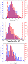 |
Fig. 5. Histograms of the dominant frequency of observed (k, m) = (0, 1) modes revealing an amplitude above 4 mmag (top), of the near-core rotation frequency frot (middle), and of the spin parameter of the dominant mode (bottom) for the Kepler sample from Li et al. (2020, blue, left y-axis) and for our Gaia sample using Eq. (4) (red, right y-axis). The red dash-dotted and dashed lines mark the lower and upper boundaries for the Gaia sample, following from our selection criterion demanding that fdom ∈ [0.7, 3.2] d−1. |
Recall that we purposefully excluded the low-frequency regime in the recipe, because the ultra-slow rotators among the gravity-mode pulsators do not comply with the linear relationship in Eq. (4). The dominant mode of all the 2497 Gaia gravity-mode pulsators thus has a spin parameter placing it into the sub-inertial regime. The values shown in the bottom panel of Fig. 5 are in line with those of the 63 best characterised Kepler pulsators with spin parameters, Rossby numbers, and stiffness values in Aerts et al. (2021).
At the high frequency end, we excluded stars with fdom above 3.2 d−1, reflected by the shorter tail in the distribution of the spin parameter in the bottom panel of Fig. 5. We thus find by construction that none of the isolated gravity-mode pulsators in our Gaia sample of field stars are expected to rotate close to their critical rate, justifying the use of the TAR for the recipe in Eq. (4). We quantify this qualitative statement in Sect. 4. Here, we just note that at least some of the γ Dor pulsators still embedded in their birth cluster are known to rotate faster, as was found for the ∼100 Myr-old young open cluster NGC 2516. Li et al. (2024) identified 11 gravity-mode pulsators in this cluster and found most of them to have near-core rotation frequencies frot ≃ 3 d−1, which is faster than the rotation rates we find for the population of isolated galactic Gaia field pulsators.
In Fig. 6 we place the stars in the Hertzsprung-Russell (HR) diagram by colour-coding their markers according to their frot and Π0(n + αg) values. The pulsators cover a broad range in effective temperature and luminosity, reflecting a wide range in stellar masses, which we determine in Sect. 4. While the near-core rotation rates and scaled buoyancy radii of the stars hotter than 8500 K appear to be randomly distributed, those of the stars within the γ Dor instability region (shown in the inset) seem to correlate with log Teff, in such a way that frot and Π0(n + αg) decrease and increase with log Teff, respectively.
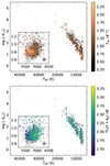 |
Fig. 6. Our sample of 2497 Gaia DR3 gravity-mode pulsators in the HR diagram. The markers are coloured according to their frot (top) and Π0(n + αg) values (bottom). Other stars of the sample of 15 692 pulsators from Mombarg et al. (2024a) are shown by the grey markers. The inset axes show close-ups of the γ Dor instability region. Typical 3σ (average) error margins are shown by the black bars in the inset. |
The 26 best modelled Kepler SPB stars did not reveal any correlation between log Teff and the dominant oscillation mode frequency, in line with earlier ground-based studies of 13 SPB pulsators (see Supplementary Material of Pedersen et al. 2021). We confirmed this conclusion for the much larger Gaia sample. This followed from simple linear regression analyses of the form y = a log Teff + b, where y is taken to be fdom, frot, and Π0(n + αg), respectively. We also repeated the regression for the inverse quantities and for the 10-base logarithm. We dedicated Appendix A to illustrate how these three seismic quantities relate to the effective temperature for our Gaia sample. These relationships are graphically depicted in the three scatter plots in Fig. A.1 for SPB stars and illustrate the lack of any correlation for these pulsators. The linear regressions applied to all the stars above the γ Dor instability strip have insignificant coefficients (a, b) for all of fdom, frot, and Π0(n + αg).
As for the γ Dor mass regime, Li et al. (2020, their Fig. 15) did not find any correlation between the oscillation periods of the (k, m) = (0, 1) modes and log Teff for their sample of Kepler γ Dor stars. No clear correspondence between Π0 and log Teff was found either. We did find weak correlations from our much larger Gaia sample but the comparisons are not equivalent. Indeed, Li et al. (2020) were able to identify the radial orders of the modes from detected period spacing patterns for each of the pulsators. For our work, we did not have any information on the radial order n of the dominant mode, so we could not make use of the buoyancy radius Π0 itself. Rather, we had to use a scaled value including the unknown factor (n + αg). Because we expected weak correlations between the seismic quantities and log Teff at best, we computed Pearson’s correlation coefficients and conducted linear regressions with Monte Carlo sampling analyses for 10 000 iterations to assess the uncertainties. We selected the stars with Teff values between 6810 K and 7540 K following the local target density in the HR diagram in Fig. 6 to ensure there to be at least 3 sample stars per 10 K within this Teff range. In each iteration, we sampled new values for log Teff, fdom, frot, and Π0(n + αg) for 85% of the selected targets and fitted linear, inverse, and logarithmic relations using Theil-Sen estimators (e.g. Theil 1950; Sen 1968). The results are summarised in Table 1 and visualised in Fig. A.2, where we point out that the dearth of stars in the upper panel at fdom, ≥ 4 mmag ≃ 1 d−1 is due to the spectral window of the TESS data as illustrated by Hey & Aerts (2024). Although the R2 values are low, as anticipated from the earlier Kepler results by Li et al. (2020), we find that fdom, frot, and Π0(n + αg) all correlate modestly but significantly with log Teff. The positive a values in Table 1 point to a positive correlation between fdom and log Teff, and by implication also between frot and log Teff. These are well visible in Fig. A.2. On the other hand, the negative a value for Π0(n + αg) points to an anti-correlation with log Teff (see bottom panel of Fig. A.2). The weaker correlation occurs because of the wider asymmetrical confidence regions for this quantity as revealed in Fig. 3.
Regression coefficients for y = a log Teff + b.
While the gravity-mode pulsators above the γ Dor instability region cover a wide range of stellar masses (Mombarg et al. 2024a, see also Sect. 4), those inside the narrow instability region have similar mass. This allowed us to probe the evolution of these stars more easily (e.g., Mombarg et al. 2021; Fritzewski et al. 2024a) than the one of the less populated SPB sample. The modest yet significant linear decrease of frot as log Teff decreases for the γ Dor pulsators offers observational input to evaluate angular momentum transport theories and simulations as these stars evolve along the main sequence (e.g. Ouazzani et al. 2019; Aerts et al. 2019; Aerts 2021). Even if we could compute more complex statistical models than the simple linear ones used here, we refrained from doing so as long as we do not have the outcome of forward modelling based on fitting individual identified modes from grids of models with a variety of input physics as done for SPB stars by Pedersen et al. (2021). Indeed, Li et al. (2020, their Fig. 16) have illustrated that the connection between frot, Π0 and Teff is complex and depends on the details of transport processes in the stellar interior as the stars evolve. We plan to achieve more advanced asteroseismic and statistical modelling in future work, by fully exploiting a considerable number of the identified modes from the TESS light curves of suitable γ Dor pulsators, rather than working with only the dominant mode as done here for the large Gaia sample. The results in Table 1 are promising to undertake such time-consuming modelling in the future.
Finally, even if the correlation is weak, we found that the scaled buoyancy radius Π0(n + αg) increases with decreasing log Teff. This is contrary to Π0 itself, which decreases as the star cools (e.g. Mombarg et al. 2019; Ouazzani et al. 2019). We thus found observational evidence of an increase in the radial order of the dominant excited mode as the γ Dor stars evolve.
4. Grid-based forward modelling
Mombarg et al. (2024b) and Fritzewski et al. (2024a) illustrated how measured values of the near-core rotation frequency and Π0 provide useful extra constraints, in addition to the luminosity and effective temperature of a star, for stellar modelling based on evolutionary tracks. In these two studies, the modelling had the purpose of determining the stellar mass M⋆, the core overshooting leading to mcc, and the age via its proxy Xc/Xini. Such evolutionary modelling is a lot less cumbersome (but also less powerful) than detailed asteroseismic modelling of individual mode frequencies (e.g. Moravveji et al. 2015, 2016; Mombarg et al. 2020, 2021; Pedersen et al. 2021). This simplified evolutionary modelling by Mombarg et al. (2024b) and Fritzewski et al. (2024a) was done by relying on grids of stellar evolution models calibrated to γ Dor star asteroseismology computed by Mombarg (2023).
In recent applications of gravity-mode asteroseismic modelling, the near-core rotation frequency of the star was derived from 4-years long Kepler light curves. These typically lead to much better precision for frot compared to the precision of ∼20% we achieved here from applying Eq. (4) to the measured fdom, after identification of the mode as (k, m) = (0, 1) in the sub-inertial regime. For the current study, we investigated whether the addition of an estimated near-core rotation frequency from just the dominant pulsation frequency helps constrain the fundamental stellar parameters M⋆, mcc, R⋆, and Xc/Xini.
We applied the same methodology as presented in Mombarg et al. (2024a), where a conditional neural flow trained on a grid of rotating stellar evolution models computed with MESA (Paxton et al. 2011, 2013, 2015, 2018, 2019; Jermyn et al. 2023) was used as an interpolator. We refer to Mombarg et al. (2024a) for the details on how this methodology works. For the sub-sample of stars with a measured frot obtained in this work, we re-derived their M⋆, mcc, R⋆, and Xc/Xini by adding frot as a third observational constraint, in addition to the two observables log Teff and log(L/L⊙) used for the modelling by Mombarg et al. (2024a). As in that paper, we relied on two extensive grids of stellar models, for values of the metallicity equal to Z = 0.0045 ([M/H]= − 0.5) and Z = 0.014 ([M/H] = 0.0). These two metallicities were chosen because we do not have a homogeneously derived measurement of the metallicity for all the sample stars. The two grids encapsulate the measured range of Z for gravity-mode pulsators having a metallicity estimate from high-resolution ground-based spectroscopy (Gebruers et al. 2021) and from Gaia spectroscopy (de Laverny et al. 2024). In addition to these two grids from Mombarg et al. (2024a), we computed a third grid for Z = 0.008 ([M/H]= − 0.25) and trained a conditional neural flow on this grid, following the same methodology as described in that paper. From the perspective of position in the HR diagram, 2375 pulsators were covered by the lowest-metallicity grid, 2439 by the intermediate-metallicity grid and 2464 by the solar metallicity grid. We worked with these stars from here onwards.
Figure 7 shows the difference in the derived fundamental stellar quantities depending on whether frot is included as an additional constraint or not, for the 2464 pulsators captured by the solar metallicity grid. As can be seen in the top-left panel, the derived stellar mass is consistent between the two cases. The largest scatter is observed in the evolutionary stage (Xc/Xini, bottom-left panel), which is harder to constrain than the mass as it depends strongly on (unknown) element mixing in the models. In the context of ensemble modelling of gravity-mode pulsators, we found that frot derived from Eq. (4) applied to the Gaia light curves helps to refine the determination of the evolutionary stage of the star from rotating stellar models. Furthermore, with the inclusion of frot, we achieved slightly more precise estimates of Xc/Xini, going from average (absolute) uncertainties of 0.10−0.08 to 0.08−0.06. In case of the convective core mass (top-right panel) and radius (bottom-right panel), the majority of the stars with the largest difference still have measurements consistent within the 68% confidence interval. The average uncertainties mcc/M⋆ and log(R⋆/R⊙) remain approximately the same when frot is included in the modelling or not. This re-affirmed that estimation of frot can be decoupled from forward asteroseismic modelling as emphasised by Van Reeth et al. (2016), Ouazzani et al. (2017) and Aerts et al. (2018).
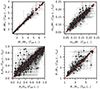 |
Fig. 7. Derived measurements for the stellar mass (top left), the fractional convective core mass (top right), the core hydrogen-mass fraction compared to the initial hydrogen-mass fraction (bottom left), and the stellar radius (bottom right) of the 2464 gravity-mode pulsators modelled via the grid with solar metallicity. The quantities on the abscissa are derived using the effective temperature and luminosity as input, while for the quantities on the ordinate, the near-core rotation frequency is added as an extra observable. The red lines indicate perfect correspondence. |
The comparative results for the 2375 pulsators covered by the lower-metallicity grids were similar, keeping in mind that the mass, luminosity, and metallicity are tightly connected for main-sequence stars (see their strong relationships deduced by Mombarg et al. 2024a). We omit them here for brevity, but they are shown visually in Figs. B.1 and B.2 in Appendix A. Given that we do not have measurements of Z for the sample stars, we provide the stellar parameters for the three grids in electronic format at the CDS, following the format in Tables B.1, B.2, and B.3 (see also footnote to the title of the paper).
The differences in the stellar parameters deduced from the grid modelling for the stars treated by the three grids reflect the systematic uncertainties for the (core) masses, radii, and evolutionary stages induced solely by the differences of 0.0060 and 0.0095 in Z (−0.25 and −0.50 in [M/H]). Again, these differences are systematic and follow the tight (core) mass – luminosity – radius – metallicity relationships. They range up to 0.55 M⊙ in mass, up to 0.28 M⊙ in convective core mass, and from about −0.25 R⊙ to +0.25 R⊙ in radius. By construction, the evolutionary stages differ from each other because the grid having Z = 0.0045 was built up by Mombarg et al. (2024a) to make sure all observed stars are above the ZAMS and to encapsulate the range in unknown metallicity reported in the literature for gravity-mode pulsators, affecting the evolution appreciably. For the grid with Z = 0.008 the differences in Xc/Xini remain more modest for most stars, reaching up to 0.3 compared to the solar metallicity case. A visual representation of the distributions of these systematic differences for all the stars with overlapping grid solutions is shown in Fig. B.3 and reflects the well-known luminosity–mass-radius–metallicity relationships for main-sequence stars (cf. Mombarg et al. 2024a).
Finally, we also studied the effect of having the higher-precision input of frot from the slope of a period-spacing pattern of dipole prograde modes based on 4-year Kepler light curves instead of the value based on just fdom from Gaia DR3 light curves. We considered the 105 Kepler pulsators from Li et al. (2020) and Pedersen et al. (2021) used to construct Eq. (4) and shown in Fig. 1. We computed their luminosity and effective temperature in the same way as we did it for the Gaia sample and found 96 of the γ Dor stars with dominant (k, m) = (0, 1) mode to be covered by the model grid with solar metallicity, while 3 of the SPB stars. We show the results of the grid modelling based on the less precise Gaia frot and the more precise Kepler frot estimates for these 99 Kepler pulsators in Fig. 8. The four estimated parameters have very consistent values for almost all 99 pulsators.
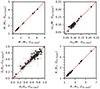 |
Fig. 8. Derived measurements for the stellar mass (top left), the fractional convective core mass (top right), the core hydrogen-mass fraction compared to the initial hydrogen-mass fraction (bottom left), and the stellar radius (bottom right) of 96 γ Dor stars (circles) and three SPB stars (squares) modelled via the grid with solar metallicity. The quantities are derived using the effective temperature, luminosity, and near-core rotation frequency from the dominant dipole prograde mode detected in the Gaia DR3 light curves (x-axis) versus the higher-precision value deduced from the slope of a period spacing pattern of dipole prograde modes of consecutive radial order following Li et al. (2020) and Pedersen et al. (2021) (y-axis). |
Having deduced the stellar parameters from grid modelling, we are now able to come back to one of the main assumptions in our procedure, namely that the pulsators may rotate fast, yet such that the centrifugal force can still be neglected. The centrifugal force affects both the equilibrium models and the pulsation computations. The former become oblate spheroids rather than spheres, while the modes will not only get affected by the Coriolis force but as well by the centrifugal force ∼Ω2. To evaluate the impact on the equilibrium models, we tested at which fraction of the critical rotation rate the stars are rotating. We note that different definitions for the critical rotation rate are used in the literature, notably the Kepler and Roche critical rate. In practical applications, these differ by a factor up to 1.84 due to the use of the equatorial or polar radius of the star at the critical rate (see Rieutord et al. 2016; Aerts & Tkachenko 2024, for discussions). Here, we worked with the cyclic Kepler critical rotation rate defined as  and assumed the derived radii of the stars to correspond with their equatorial value. This is an appropriate choice since we are dealing with stars having a dominant sectoral dipole mode in an observer’s frame, which favours a more equator-on than pole-on view. We then used the mass result from the grid modelling to compute frot/fcrit for all the pulsators in our Gaia sample. The values ranged from 0.7% to 25% and imply that the stars are not strongly deformed by the rotation according to the asteroseismic validity criteria for prograde modes adopted by Ballot et al. (2012) and Ouazzani et al. (2017). The latter authors, as well as Ballot et al. (2013) concluded that the centrifugal force can safely be ignored for the calculation of prograde dipole gravity modes when frot/fcrit < 40%, which is fulfilled for all our sample stars. This justifies the use of the TAR also from the perspective of the stellar deformation due to the rotation.
Overall, our results reveal the great potential of using Eq. (4) to deduce frot and grid-based stellar parameter estimation based on just the value of the dominant mode frequency from Gaia light curves along with the effective temperature and luminosity. All these quantities are homogeneously computed and available from Gaia DR3 (and its future Data Releases DR4 and DR5). When coupled to an asteroseismically calibrated grid of stellar models as those in Mombarg et al. (2024a) and used here, these observables deliver stellar parameters calibrated by the star’s internal properties via the observed dominant mode frequency. The only requirement for the procedure to work is the ability to identify pulsators with a dominant dipole prograde mode having its frequency in the frame co-rotating with the star, fco, in the sub-inertial regime of the frequency spectrum (spin parameter ν = 2 ⋅ frot/fco > 1), while ensuring a modest rotational deformation of frot/fcrit < 40%.
5. Near-core to surface rotation estimates
5.1. Evolution of the near-core rotation
Combining the results of the previous two sections, we studied the near-core rotation frequency as a function of evolutionary stage. Asteroseismology has demonstrated that angular momentum transport from the deep interior to the envelope of stars happens more efficiently than anticipated from theories of transport processes adopted prior to the era of space asteroseismology (Ouazzani et al. 2019). It was also found that gravity-mode pulsators have low levels of near-core to surface rotation (Aerts et al. 2019; Li et al. 2020; Aerts 2021; Aerts & Tkachenko 2024, for observational summaries). Moreover, stars born with a radiative envelope lose angular momentum rapidly beyond the TAMS (at Xc/Xini = 0), while their near-core rotation drops appreciably (Aerts 2021, Fig. 6).
In Fig. 9, we show the model-independent near-core rotation frequency, frot, as a function of the model-dependent evolutionary stage for our sample of gravity-mode pulsators, for the three grids. Thanks to the four times larger size of our Gaia population of pulsators with a measurement of frot compared to the Li et al. (2020)Kepler sample, and to our estimate of the evolutionary stage, we see a clear decline of the average near-core rotation frequency of the population as the stars evolve.
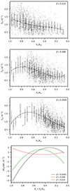 |
Fig. 9. Inferred near-core rotation frequencies of the Gaia gravity-mode pulsators plotted as a function of evolutionary stage (grey dots), assuming solar metallicity (2464 stars, top panel), [M/H] = −0.25 (2439 stars, second panel), and [M/H] = −0.5 (2375 stars, third panel). Solid lines indicate spline fits through binned averages (see text). The bottom panel shows the derivatives of the splines from the three upper panels, indicating the change in the near-core rotation frequency with respect to the fraction of hydrogen in the core. The dotted grey line separates positive and negative values. |
We fitted uni-variate splines through bin-averaged frot values, where we selected the optimal bin size in Xc′=Xc/Xini according to Scott’s rule (Scott 1979). This rule states that a histogram with bin size proportional to  , where Npoints is the number of points in the bins and σ the standard deviation assuming a normal distribution, is very efficient in approaching the true distribution. The smoothing factor for the splines was chosen such that higher values do no longer change the resulting derivative dfrot/dXc′. The derivatives of the fitted splines are shown in the bottom panel of Fig. 9. When assuming Z = 0.014, we found purely decreasing frot values during the main sequence. Despite the large range of near-core rotation frequencies per evolutionary stage – reflecting the variety of initial conditions at birth for this population of field stars – the average near-core rotation per bin in Xc/Xini shows a gradual decline from the zero-age to the terminal-age main sequence, with roughly a factor of two.
Assuming Z = 0.0045, the results were less clear. We found that stars on average have an increasing frot (negative derivative) during the first part of the main sequence, followed by a decrease in frot. Yet, we note that the part where dfrot/dXc′ < 0 for Z = 0.0045 is severely undersampled and so we could not rely on these results. However, the same decline of frot with a factor two as for the solar metallicity grid was obtained for the regime Xc/Xini < 0.5 when the stars are modelled with the metal-poor grid. When assuming Z = 0.008, a similar trend in dfrot/dXc′ is observed.
Finally, we checked that the trends found become less clear but do not change globally when we split up the observed sample in stars with an initially growing convective core and stars whose convective core shrinks as of the ZAMS. The distinction between these two cases happens for masses between about 1.6 M⊙ and 1.8 M⊙, depending on the metallicity. We therefore conclude to have found observational evidence that the near-core rotation frequency of isolated gravity-mode field pulsators in the Milky Way decreases with a factor of about two by the time they will reach the TAMS if we consider all the well covered bins in Fig. 9, irrespective of the initial metallicity.
5.2. Limits on the surface rotation
Only 58 of the Kepler γ Dor stars also have a value for the surface rotation, measured from rotational modulation (Van Reeth et al. 2018; Li et al. 2020) and only 22 have a measurement of their averaged envelope rotation, fenv, determined from identified rotational splitting (Kurtz et al. 2014; Saio et al. 2015; Keen et al. 2015; Li et al. 2019). For the SPB stars, information is even more restricted, with only one star having clear rotational splitting (Pápics et al. 2014) and a rotational profile throughout the star from frequency inversions (the 3.3 M⊙ SPB KIC 10526294, Triana et al. 2015). These limited observational constraints on differential near-core to surface rotation in main-sequence stars of intermediate and high mass (as summarised by Aerts 2021, Fig. 6) restrict our ability to improve angular momentum transport theories, as these rely on the gradient of the rotation profile throughout the star (Ouazzani et al. 2019; Aerts et al. 2019).
We were unable to assess the envelope or surface rotation from the Gaia light curves. However, we derived a lower limit for the cyclic surface rotation frequency, fsurf, from the radius estimates shown in Fig. 7 for those stars with a measurement of the spectral line broadening offered by the Gaia spectroscopy (Frémat et al. 2023). Aerts et al. (2023) showed the Gaiavbroad parameter to capture the joint effect of time-independent rotational line broadening and time-dependent tangential pulsational broadening due to gravity modes. Moreover, pulsational line broadening of gravity-mode pulsators is typically only a small fracion of the rotational broadening for moderate to fast rotators (De Cat & Aerts 2002; Aerts et al. 2004; De Cat et al. 2006). Hence Gaia’s vbroad measurement is a meaningful approximation of 2πR⋆ ⋅ fsurf ⋅ sin i for such stars, where i is the (unknown) inclination angle of the rotation axis of the star in the line-of-sight.
A total of 969 of our sample stars have a significant vbroad measurement, by which we mean it is above zero at 1-σ level, and a radius estimate from the solar metallicity grid. For the lower-metallicity grids it concerns 965 stars for Z = 0.008 and 929 stars for Z = 0.0045. Using the radius estimates from the grid modelling, we computed fsurf ⋅ sin i from vbroad. As this is a lower limit for the true surface rotation frequency fsurf, we obtained an upper limit for the near-core to surface differential rotation from calculating frot/(fsurf ⋅ sin i). Our results are illustrated in Fig. B.4 and reveal values up to 5.4, irrespective of the assumption about the metallicity. The upper limits shown in Fig. B.4 have large uncertainty (up to 100%) for many of the stars due to the large errors of vbroad (not shown in the figure for visibility reasons). So far, asteroseismology of single γ Dor stars covering the mass range [1.3, 1.9] M⊙ has shown them all to have quasi-rigid rotation at the level of frot/fsurf ∈ [0.9, 1.1] if such a measurement is available (Li et al. 2020; Aerts 2021, for a summary). Our work increases the mass range of stars with an estimate of differential rotation, even if we can provide only an upper limit. Indeed, of the 969 gravity-mode pulsators presented in Fig. B.4, 58 have a mass between 2.0 M⊙ and 4.4 M⊙ when adopting solar metallicity. The unknown factor sin i and the large uncertainty of vbroad did not allow us to deduce stricter constraints than just a rough upper limit for frot/fsurf. Measurements of the actual ratio frot/fenv can be investigated from detailed analyses of the TESS light curves for the hybrid low-order pressure and high-order gravity mode pulsators in our sample. This will be taken up in future work.
6. Conclusions and outlook
In this work, we derived the internal rotation frequency of 2497 gravity-mode pulsators discovered recently from Gaia DR3 light curves. These field stars cover the mass range from 1.3 M⊙ to about 7 M⊙ and the entire main sequence. We provide an easy-to-apply procedure to deduce their near-core rotation frequency. Our linear regression recipe is based on the dominant prograde dipole oscillation mode found in the Gaia DR3 light curves. The 2497 Gaia pulsators have near-core rotation rates ranging from 0.3 d−1 (≃3.5 μHz) to 2.4 d−1 (≃27.8 μHz), with a distribution in line with those of Kepler gravity-mode pulsators. All these Gaia pulsators have an identified dominant dipole prograde mode in the sub-inertial frequency regime with spin parameters ranging from about 2 to 6. They cover a ratio of the near-core rotation rate to the Keplerian critical rate from 0.7% to 25%. Their stellar parameters were deduced from asteroseismically calibrated grids of rotating stellar models. With our work, we quadruple the sample size of intermediate-mass dwarfs with a measurement of the near-core rotation frequency in the transition layer between the convective core and the radiative envelope.
The weakest point of the grid modelling performed for the Gaia sample is the quite large uncertainty for the evolutionary stage of the stars, quantified as the central hydrogen mass fraction over the initial value, Xc/Xini. The reason is that we do not have a good estimate of the initial metallicity of the pulsators, preventing us to assign an age to the stars based on their Xc/Xini value. This can perhaps be overcome from future detailed asteroseismic modelling based on a measurement of abundances from high-resolution spectroscopy coupled to the fitting of numerous identified oscillation mode frequencies from grids of stellar models built with a variety of choices for the input physics. The study by Pedersen et al. (2021) is so far the only one that achieved such an asteroseismic age calibration for gravity-mode pulsators on the main sequence. The authors considered eight grids of models with different input physics for the transport processes, but their study only covered 26 modelled SPB stars. Future similar work for a large sample with the most promising among our Gaia pulsators from their complete list of significant TESS oscillation frequencies is on the horizon.
For 969 pulsators in the sample, we derived an upper limit of the radial differential rotation between the boundary of the convective core and the surface, by relying on the Gaia DR3 vbroad observable combined with the radius estimate from the grid modelling. We find values up to 5.4. These results cover the mass range of [1.3, 4.4] M⊙ and constitute an interesting sub-sample to calibrate stellar evolution theory and angular momentum transport theories for rotating main-sequence stars with a convective core and a radiative envelope. This is of particular interest during the initial ∼20% of the main sequence. In order to understand such early phases of stellar evolution, it is needed to deduce high-precision values for Xc/Xini. An excellent way to achieve this, as well as calibrate age-dating from Xc/Xini, is to perform asteroseismic modelling of gravity-mode pulsators in detached binaries and/or open clusters. Such modelling work was done for a few binaries (Schmid & Aerts 2016; Sekaran et al. 2021; Kemp et al. 2024) and also for the open cluster UBC 1 (Fritzewski et al. 2024b). It is currently ongoing for the very young (≃100 Myr) open cluster NGC 2516, in which Li et al. (2024) discovered 9 γ Dor and 2 SPB pulsators rotating at half their critical Keplerian rotation rate. This is a higher internal rotation regime than the one covered by our sample of Gaia field pulsators.
Finally, we point to the large potential of future Gaia data releases. Combining these data with high-cadence high-precision space photometry from the ongoing TESS and future PLATO (Rauer et al. 2024) missions will allow us to scale up the work presented here to millions of pulsators, instead of thousands. Our recipe in Eq. (4) to deduce the near-core rotation of pulsators with a dominant prograde dipole gravito-inertial mode having a mass above 1.3 M⊙ is suitable to facilitate fast asteroseismic grid modelling. At the same time, it is also a particularly handy and relevant tool for exoplanet host studies in terms of the angular momentum properties of the hottest among the main-sequence star-planet systems.
Data availability
The full Tables B.1–B.3 are available at the CDS via anonymous ftp to cdsarc.cds.unistra.fr (130.79.128.5) or via https://cdsarc.cds.unistra.fr/viz-bin/cat/J/A+A/695/A214
Acknowledgments
We thank the referee for the useful detailed suggestions, which helped us to improve the presentation of our work. CA is grateful to Maarten Dirickx, Toon De Prins and Thomas Ceulemans for helping her with compiler issues. The research leading to these results has received funding from the KU Leuven Research Council (grant C16/18/005: PARADISE) and from the European Research Council (ERC) under the Horizon Europe programme (Synergy Grant agreement N°101071505: 4D-STAR). While partially funded by the European Union, views and opinions expressed are however those of the authors only and do not necessarily reflect those of the European Union or the European Research Council. Neither the European Union nor the granting authority can be held responsible for them. CA also acknowledges the Belgian Federal Science Policy Office (BELSPO) for their financial support in the framework of the PRODEX Programme of the European Space Agency (ESA), facilitating the exploitation of the Gaia data. JSGM acknowledges funding fron the French Agence Nationale de la Recherche (ANR), under grant MASSIF (ANR-21-CE31-0018-02). The authors appreciated valuable comments from Dominic Bowman, Dario Fritzewski, and Mathijs Vanrespaille on an early version of the manuscript.
References
- Aerts, C. 2021, Rev. Mod. Phys., 93, 015001 [Google Scholar]
- Aerts, C., & Tkachenko, A. 2024, A&A, 692, R1 [NASA ADS] [CrossRef] [EDP Sciences] [Google Scholar]
- Aerts, C., Cuypers, J., De Cat, P., et al. 2004, A&A, 415, 1079 [NASA ADS] [CrossRef] [EDP Sciences] [Google Scholar]
- Aerts, C., Christensen-Dalsgaard, J., & Kurtz, D. W. 2010, Asteroseismology (Heidelberg: Springer-Verlag) [Google Scholar]
- Aerts, C., Van Reeth, T., & Tkachenko, A. 2017, ApJ, 847, L7 [Google Scholar]
- Aerts, C., Molenberghs, G., Michielsen, M., et al. 2018, ApJS, 237, 15 [Google Scholar]
- Aerts, C., Mathis, S., & Rogers, T. M. 2019, ARA&A, 57, 35 [Google Scholar]
- Aerts, C., Augustson, K., Mathis, S., et al. 2021, A&A, 656, A121 [NASA ADS] [CrossRef] [EDP Sciences] [Google Scholar]
- Aerts, C., Molenberghs, G., & De Ridder, J. 2023, A&A, 672, A183 [NASA ADS] [CrossRef] [EDP Sciences] [Google Scholar]
- Audenaert, J., & Tkachenko, A. 2022, A&A, 666, A76 [NASA ADS] [CrossRef] [EDP Sciences] [Google Scholar]
- Ballot, J., Lignières, F., Prat, V., Reese, D. R., & Rieutord, M. 2012, ASP Conf. Ser., 462, 389 [Google Scholar]
- Ballot, J., Lignières, F., & Reese, D. R. 2013, in Lecture Notes in Physics, eds. M. Goupil, K. Belkacem, C. Neiner, F. Lignières, & J. J. Green (Berlin: Springer-Verlag), 865, 91 [NASA ADS] [CrossRef] [Google Scholar]
- Beck, P. G., Bedding, T. R., Mosser, B., et al. 2011, Science, 332, 205 [Google Scholar]
- Beck, P. G., Montalban, J., Kallinger, T., et al. 2012, Nature, 481, 55 [Google Scholar]
- Bedding, T. R., Mosser, B., Huber, D., et al. 2011, Nature, 471, 608 [Google Scholar]
- Bétrisey, J., Eggenberger, P., Buldgen, G., Benomar, O., & Bazot, M. 2023, A&A, 673, L11 [NASA ADS] [CrossRef] [EDP Sciences] [Google Scholar]
- Bouabid, M. P., Dupret, M. A., Salmon, S., et al. 2013, MNRAS, 429, 2500 [Google Scholar]
- Chaboyer, B., & Zahn, J. P. 1992, A&A, 253, 173 [NASA ADS] [Google Scholar]
- Córsico, A. H., Althaus, L. G., Miller Bertolami, M. M., & Kepler, S. O. 2019, A&ARv, 27, 7 [Google Scholar]
- Davison, A. C., & Hinkley, D. V. 1997, Bootstrap Methods and their Application, Cambridge Series in Statistical and Probabilistic Mathematics (Cambridge: Cambridge University Press) [CrossRef] [Google Scholar]
- De Cat, P., & Aerts, C. 2002, A&A, 393, 965 [NASA ADS] [CrossRef] [EDP Sciences] [Google Scholar]
- De Cat, P., Eyer, L., Cuypers, J., et al. 2006, A&A, 449, 281 [NASA ADS] [CrossRef] [EDP Sciences] [Google Scholar]
- de Laverny, P., Recio-Blanco, A., Aerts, C., & Palicio, P. A. 2024, A&A, 691, A182 [NASA ADS] [CrossRef] [EDP Sciences] [Google Scholar]
- Degroote, P., Aerts, C., Baglin, A., et al. 2010, Nature, 464, 259 [Google Scholar]
- Deheuvels, S., García, R. A., Chaplin, W. J., et al. 2012, A&A, 756, 19 [Google Scholar]
- Deheuvels, S., Doğan, G., Goupil, M. J., et al. 2014, A&A, 564, A27 [NASA ADS] [CrossRef] [EDP Sciences] [Google Scholar]
- Deheuvels, S., Ballot, J., Beck, P. G., et al. 2015, A&A, 580, A96 [NASA ADS] [CrossRef] [EDP Sciences] [Google Scholar]
- Deheuvels, S., Ballot, J., Eggenberger, P., et al. 2020, A&A, 641, A117 [EDP Sciences] [Google Scholar]
- Dhouib, H., Prat, V., Van Reeth, T., & Mathis, S. 2021a, A&A, 652, A154 [NASA ADS] [CrossRef] [EDP Sciences] [Google Scholar]
- Dhouib, H., Prat, V., Van Reeth, T., & Mathis, S. 2021b, A&A, 656, A122 [NASA ADS] [CrossRef] [EDP Sciences] [Google Scholar]
- Di Mauro, M. P., Ventura, R., Cardini, D., et al. 2016, ApJ, 817, 65 [NASA ADS] [CrossRef] [Google Scholar]
- Dupret, M.-A., Belkacem, K., Samadi, R., et al. 2009, A&A, 506, 57 [NASA ADS] [CrossRef] [EDP Sciences] [Google Scholar]
- Eggenberger, P., Deheuvels, S., Miglio, A., et al. 2019a, A&A, 621, A66 [NASA ADS] [CrossRef] [EDP Sciences] [Google Scholar]
- Eggenberger, P., den Hartogh, J. W., Buldgen, G., et al. 2019b, A&A, 631, L6 [NASA ADS] [CrossRef] [EDP Sciences] [Google Scholar]
- Eggenberger, P., Moyano, F. D., & den Hartogh, J. W. 2022, A&A, 664, L16 [NASA ADS] [CrossRef] [EDP Sciences] [Google Scholar]
- Frémat, Y., Royer, F., Marchal, O., et al. 2023, A&A, 674, A8 [NASA ADS] [CrossRef] [EDP Sciences] [Google Scholar]
- Fritzewski, D. J., Aerts, C., Mombarg, J. S. G., Gossage, S., & Van Reeth, T. 2024a, A&A, 684, A112 [NASA ADS] [CrossRef] [EDP Sciences] [Google Scholar]
- Fritzewski, D. J., Van Reeth, T., Aerts, C., et al. 2024b, A&A, 681, A13 [NASA ADS] [CrossRef] [EDP Sciences] [Google Scholar]
- Fuller, J., Piro, A. L., & Jermyn, A. S. 2019, MNRAS, 485, 3661 [NASA ADS] [Google Scholar]
- Gaia Collaboration (De Ridder, J., et al.) 2023, A&A, 674, A36 [CrossRef] [EDP Sciences] [Google Scholar]
- García, R. A., & Ballot, J. 2019, Liv. Rev. Sol. Phys., 16, 4 [Google Scholar]
- Garcia, S., Van Reeth, T., De Ridder, J., et al. 2022, A&A, 662, A82 [NASA ADS] [CrossRef] [EDP Sciences] [Google Scholar]
- Gebruers, S., Straumit, I., Tkachenko, A., et al. 2021, A&A, 650, A151 [NASA ADS] [CrossRef] [EDP Sciences] [Google Scholar]
- Gehan, C., Mosser, B., Michel, E., Samadi, R., & Kallinger, T. 2018, A&A, 616, A24 [NASA ADS] [CrossRef] [EDP Sciences] [Google Scholar]
- Guzik, J. A., Kaye, A. B., Bradley, P. A., Cox, A. N., & Neuforge, C. 2000, ApJ, 542, L57 [Google Scholar]
- Heger, A., Langer, N., & Woosley, S. E. 2000, ApJ, 528, 368 [NASA ADS] [CrossRef] [Google Scholar]
- Hekker, S., & Christensen-Dalsgaard, J. 2017, A&ARv, 25, 1 [Google Scholar]
- Henneco, J., Van Reeth, T., Prat, V., et al. 2021, A&A, 648, A97 [EDP Sciences] [Google Scholar]
- Hermes, J. J., Gänsicke, B. T., Kawaler, S. D., et al. 2017, ApJS, 232, 23 [Google Scholar]
- Hey, D., & Aerts, C. 2024, A&A, 688, A93 [NASA ADS] [CrossRef] [EDP Sciences] [Google Scholar]
- Jermyn, A. S., Bauer, E. B., Schwab, J., et al. 2023, ApJS, 265, 15 [NASA ADS] [CrossRef] [Google Scholar]
- Keen, M. A., Bedding, T. R., Murphy, S. J., et al. 2015, MNRAS, 454, 1792 [Google Scholar]
- Kemp, A., Tkachenko, A., Torres, G., et al. 2024, A&A, 689, A164 [NASA ADS] [CrossRef] [EDP Sciences] [Google Scholar]
- Kurtz, D. W. 2022, ARA&A, 60, 31 [NASA ADS] [CrossRef] [Google Scholar]
- Kurtz, D. W., Saio, H., Takata, M., et al. 2014, MNRAS, 444, 102 [Google Scholar]
- Lee, U., & Saio, H. 1987, MNRAS, 224, 513 [Google Scholar]
- Lee, U., & Saio, H. 1997, ApJ, 491, 839 [Google Scholar]
- Li, G., Bedding, T. R., Murphy, S. J., et al. 2019, MNRAS, 482, 1757 [Google Scholar]
- Li, G., Van Reeth, T., Bedding, T. R., et al. 2020, MNRAS, 491, 3586 [Google Scholar]
- Li, G., Aerts, C., Bedding, T. R., et al. 2024, A&A, 686, A142 [NASA ADS] [CrossRef] [EDP Sciences] [Google Scholar]
- Maeder, A. 2009, Physics, Formation and Evolution of Rotating Stars (Heidelberg: Springer-Verlag) [Google Scholar]
- Maeder, A., & Meynet, G. 2000, ARA&A, 38, 143 [Google Scholar]
- Mathis, S. 2013, in Transport Processes in Stellar Interiors, eds. M. Goupil, K. Belkacem, C. Neiner, F. Lignières, & J. J. Green, 865, 23 [Google Scholar]
- Mathis, S., & Prat, V. 2019, A&A, 631, A26 [NASA ADS] [CrossRef] [EDP Sciences] [Google Scholar]
- Miglio, A., Montalbán, J., Noels, A., & Eggenberger, P. 2008, MNRAS, 386, 1487 [Google Scholar]
- Mombarg, J. S. G. 2023, A&A, 677, A63 [NASA ADS] [CrossRef] [EDP Sciences] [Google Scholar]
- Mombarg, J. S. G., Van Reeth, T., Pedersen, M. G., et al. 2019, MNRAS, 485, 3248 [NASA ADS] [CrossRef] [Google Scholar]
- Mombarg, J. S. G., Dotter, A., Van Reeth, T., et al. 2020, ApJ, 895, 51 [Google Scholar]
- Mombarg, J. S. G., Van Reeth, T., & Aerts, C. 2021, A&A, 650, A58 [NASA ADS] [CrossRef] [EDP Sciences] [Google Scholar]
- Mombarg, J. S. G., Aerts, C., Van Reeth, T., & Hey, D. 2024a, A&A, 691, A131 [NASA ADS] [CrossRef] [EDP Sciences] [Google Scholar]
- Mombarg, J. S. G., Aerts, C., & Molenberghs, G. 2024b, A&A, 685, A21 [NASA ADS] [CrossRef] [EDP Sciences] [Google Scholar]
- Moravveji, E., Aerts, C., Pápics, P. I., Triana, S. A., & Vandoren, B. 2015, A&A, 580, A27 [NASA ADS] [CrossRef] [EDP Sciences] [Google Scholar]
- Moravveji, E., Townsend, R. H. D., Aerts, C., & Mathis, S. 2016, ApJ, 823, 130 [NASA ADS] [CrossRef] [Google Scholar]
- Mosser, B., Goupil, M. J., Belkacem, K., et al. 2012, A&A, 548, A10 [NASA ADS] [CrossRef] [EDP Sciences] [Google Scholar]
- Mosser, B., Benomar, O., Belkacem, K., et al. 2014, A&A, 572, L5 [NASA ADS] [CrossRef] [EDP Sciences] [Google Scholar]
- Mosser, B., Vrard, M., Belkacem, K., Deheuvels, S., & Goupil, M. J. 2015, A&A, 584, A50 [NASA ADS] [CrossRef] [EDP Sciences] [Google Scholar]
- Moyano, F. D., Eggenberger, P., Mosser, B., & Spada, F. 2023a, A&A, 673, A110 [NASA ADS] [CrossRef] [EDP Sciences] [Google Scholar]
- Moyano, F. D., Eggenberger, P., Salmon, S. J. A. J., Mombarg, J. S. G., & Ekström, S. 2023b, A&A, 677, A6 [NASA ADS] [CrossRef] [EDP Sciences] [Google Scholar]
- Moyano, F. D., Eggenberger, P., & Salmon, S. J. A. J. 2024, A&A, 681, L16 [NASA ADS] [CrossRef] [EDP Sciences] [Google Scholar]
- Ouazzani, R.-M., Salmon, S. J. A. J., Antoci, V., et al. 2017, MNRAS, 465, 2294 [Google Scholar]
- Ouazzani, R. M., Marques, J. P., Goupil, M. J., et al. 2019, A&A, 626, A121 [NASA ADS] [CrossRef] [EDP Sciences] [Google Scholar]
- Ouazzani, R. M., Lignières, F., Dupret, M. A., et al. 2020, A&A, 640, A49 [NASA ADS] [CrossRef] [EDP Sciences] [Google Scholar]
- Pamyatnykh, A. A. 1999, Acta Astron., 49, 119 [Google Scholar]
- Pápics, P. I., Briquet, M., Baglin, A., et al. 2012, A&A, 542, A55 [NASA ADS] [CrossRef] [EDP Sciences] [Google Scholar]
- Pápics, P. I., Moravveji, E., Aerts, C., et al. 2014, A&A, 570, A8 [NASA ADS] [CrossRef] [EDP Sciences] [Google Scholar]
- Pápics, P. I., Tkachenko, A., Van Reeth, T., et al. 2017, A&A, 598, A74 [Google Scholar]
- Paxton, B., Bildsten, L., Dotter, A., et al. 2011, ApJS, 192, 3 [Google Scholar]
- Paxton, B., Cantiello, M., Arras, P., et al. 2013, ApJS, 208, 4 [Google Scholar]
- Paxton, B., Marchant, P., Schwab, J., et al. 2015, ApJS, 220, 15 [Google Scholar]
- Paxton, B., Schwab, J., Bauer, E. B., et al. 2018, ApJS, 234, 34 [NASA ADS] [CrossRef] [Google Scholar]
- Paxton, B., Smolec, R., Schwab, J., et al. 2019, ApJS, 243, 10 [Google Scholar]
- Pedersen, M. G. 2022a, ApJ, 940, 49 [NASA ADS] [CrossRef] [Google Scholar]
- Pedersen, M. G. 2022b, ApJ, 930, 94 [NASA ADS] [CrossRef] [Google Scholar]
- Pedersen, M. G., Aerts, C., Pápics, P. I., et al. 2021, Nat. Astron., 5, 715 [NASA ADS] [CrossRef] [Google Scholar]
- Rauer, H., Aerts, C., Cabrera, J., et al. 2024, Exp. Astron., in press [arXiv:2406.05447] [Google Scholar]
- Rieutord, M., Espinosa Lara, F., & Putigny, B. 2016, J. Comput. Phys., 318, 277 [NASA ADS] [CrossRef] [Google Scholar]
- Saio, H., Kurtz, D. W., Takata, M., et al. 2015, MNRAS, 447, 3264 [Google Scholar]
- Saio, H., Kurtz, D. W., Murphy, S. J., Antoci, V. L., & Lee, U. 2018, MNRAS, 474, 2774 [Google Scholar]
- Saio, H., Takata, M., Lee, U., Li, G., & Van Reeth, T. 2021, MNRAS, 502, 5856 [Google Scholar]
- Schmid, V. S., & Aerts, C. 2016, A&A, 592, A116 [NASA ADS] [CrossRef] [EDP Sciences] [Google Scholar]
- Scott, D. W. 1979, Biometrika, 66, 605 [CrossRef] [Google Scholar]
- Sekaran, S., Tkachenko, A., Abdul-Masih, M., et al. 2020, A&A, 643, A162 [EDP Sciences] [Google Scholar]
- Sekaran, S., Tkachenko, A., Johnston, C., & Aerts, C. 2021, A&A, 648, A91 [NASA ADS] [CrossRef] [EDP Sciences] [Google Scholar]
- Sen, P. K. 1968, J. Am. Stat. Assoc., 63, 1379 [CrossRef] [Google Scholar]
- Sepulveda, A. G., Huber, D., Zhang, Z., et al. 2022, ApJ, 938, 49 [NASA ADS] [CrossRef] [Google Scholar]
- Sepulveda, A. G., Huber, D., Li, G., et al. 2023, Res. Notes Am. Astron. Soc., 7, 2 [Google Scholar]
- Szewczuk, W., & Daszyńska-Daszkiewicz, J. 2017, MNRAS, 469, 13 [NASA ADS] [CrossRef] [Google Scholar]
- Szewczuk, W., & Daszyńska-Daszkiewicz, J. 2018, MNRAS, 478, 2243 [Google Scholar]
- Szewczuk, W., Walczak, P., & Daszyńska-Daszkiewicz, J. 2021, MNRAS, 503, 5894 [NASA ADS] [CrossRef] [Google Scholar]
- Theil, H. 1950, A Rank-Invariant Method of Linear and Polynomial Regression Analysis I, II, III. Proceedings of the Koninklijke NederlandseAkademie van Wetenschappen, 53, 386–392, 521–525, 1397–1412 [Google Scholar]
- Townsend, R. H. D. 2003, MNRAS, 340, 1020 [Google Scholar]
- Triana, S. A., Moravveji, E., Pápics, P. I., et al. 2015, ApJ, 810, 16 [Google Scholar]
- Triana, S. A., Corsaro, E., De Ridder, J., et al. 2017, A&A, 602, A62 [NASA ADS] [CrossRef] [EDP Sciences] [Google Scholar]
- Van Reeth, T., Tkachenko, A., Aerts, C., et al. 2015a, ApJS, 218, 27 [Google Scholar]
- Van Reeth, T., Tkachenko, A., Aerts, C., et al. 2015b, A&A, 574, A17 [NASA ADS] [CrossRef] [EDP Sciences] [Google Scholar]
- Van Reeth, T., Tkachenko, A., & Aerts, C. 2016, A&A, 593, A120 [NASA ADS] [CrossRef] [EDP Sciences] [Google Scholar]
- Van Reeth, T., Mombarg, J. S. G., Mathis, S., et al. 2018, A&A, 618, A24 [NASA ADS] [EDP Sciences] [Google Scholar]
- Wu, T., Li, Y., Deng, Z.-M., et al. 2020, ApJ, 899, 38 [NASA ADS] [CrossRef] [Google Scholar]
- Xiong, D. R., Deng, L., Zhang, C., & Wang, K. 2016, MNRAS, 457, 3163 [Google Scholar]
- Zahn, J. P. 1992, A&A, 265, 115 [NASA ADS] [Google Scholar]
Appendix A: Correlations between seismic quantities and the effective temperature
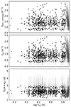 |
Fig. A.1. Dominant mode frequency (top), inferred near-core rotation frequency frot (middle), and Π0(n + αg) (bottom) plotted as a function of log Teff for pulsators above (black) and within (grey) the γ Dor instability region. |
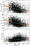 |
Fig. A.2. Same as Fig. A.1 but for pulsators within (black) and outside (grey) the γ Dor instability region. The orange, cyan, and red lines show the results of inverse, logarithmic, and linear regression analyses for the black dots with coefficients listed in Table 1, respectively. |
Appendix B: Extra figures and tables for Sect. 4
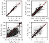 |
Fig. B.1. Similar to Fig. 7, but for the 2,375 gravity-mode pulsators modelled via the [M/H]= − 0.5 grid. |
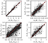 |
Fig. B.2. Similar to Fig. 7, but for the 2,439 gravity-mode pulsators modelled via the [M/H]= − 0.25 grid. |
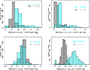 |
Fig. B.3. Differences in estimates from the grid modelling for the mass (upper left), convective core mass (upper right), radius (lower left), and evolutionary stage (lower right) due to the change in metallicity. The differences arise from the values for Z = 0.014 minus those for Z = 0.008 (grey) and Z = 0.0045 (cyan), respectively. |
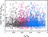 |
Fig. B.4. Upper limits for the near-core to envelope rotation rate deduced from Gaia DR3 measurements of vbroad available for 969, 965, and 929 gravity-mode pulsators in the sample of pulsators with a radius estimate from the Z = 0.014 (grey triangles), Z = 0.0080 (pink circles), and Z = 0.0045 (blue diamonds) model grids, respectively. |
Parameters of the gravity-mode pulsators covered by the solar metallicity grid.
Same as Table B.1 but for the grid having Z = 0.0080.
Same as Table B.1 but for the grid having Z = 0.0045.
All Tables
Parameters of the gravity-mode pulsators covered by the solar metallicity grid.
All Figures
|
Fig. 1. Near-core rotation frequency frot plotted as a function of dominant mode frequency for Kepler gravity-mode pulsators having an observed amplitude above 4 mmag (fdom, ≥ 4 mmag) from the samples of Li et al. (2020) and Pedersen et al. (2021). Stars are drawn as γ Dor pulsator if they have Teff < 8500 K and Π0 < 0.7 d and as SPB star otherwise. When invisible, the error bars are smaller than the symbol sizes. The linear relation (red line) given by Eq. (4) was computed for the 105 stars having a dominant (k, m) = (0, 1) mode with observed frequency above 0.35 d−1 and with ν > 1 (full symbols). The shaded area shows the 1-σ uncertainty region for this relation. The two pulsators indicated in cyan come from short CoRoT light curves (Degroote et al. 2010; Pápics et al. 2012). As the other open symbols, they were not used in the regression. The dashed (dotted) lines mark the 1-σ confidence interval for frot derived from the residuals with respect to the red line, excluding (including) stars with modes having (k, m)≠(0, 1) or ν < 1. |
| In the text | |
|
Fig. 2. Residuals from the linear fit described by Eq. (4) for the selected Kepler pulsators used in Fig. 1. The distribution of modes with (k, m) = (0, 1), ν > 1, and observed frequency above 0.35 d−1 is shown in dark grey, wile the distribution of all dominant modes with amplitude ≥4 mmag is shown in light grey. The full, dashed, and dotted lines indicate the same relation and confidence intervals as those in Fig. 1. |
| In the text | |
|
Fig. 3. The quantity Π0(n + αg) plotted as a function of the dominant prograde dipole gravity-mode frequency with amplitude above 4 mmag (fdom, ≥ 4 mmag) for 105 γ Dor and SPB stars from Li et al. (2020) and Pedersen et al. (2021). The symbols have the same meaning as in Fig. 1. The relation given by Eq. (3) is shown by the red line, while the shaded area shows the 1-σ uncertainty region. The dashed lines mark the 1-σ confidence region, propagated forward from the confidence regions of the frot values. |
| In the text | |
|
Fig. 4. Stacked periodogram of the 2497 sample stars calculated for the TESS light curves from Hey & Aerts (2024). Each row corresponds to the amplitude spectrum of one star in the gravity-mode sub-sample treated here, sorted by the dominant mode period. For all these 2497 pulsators, the dominant mode period occurs in the ridge of prograde dipole gravito-inertial (k, m) = (0, 1) modes. |
| In the text | |
|
Fig. 5. Histograms of the dominant frequency of observed (k, m) = (0, 1) modes revealing an amplitude above 4 mmag (top), of the near-core rotation frequency frot (middle), and of the spin parameter of the dominant mode (bottom) for the Kepler sample from Li et al. (2020, blue, left y-axis) and for our Gaia sample using Eq. (4) (red, right y-axis). The red dash-dotted and dashed lines mark the lower and upper boundaries for the Gaia sample, following from our selection criterion demanding that fdom ∈ [0.7, 3.2] d−1. |
| In the text | |
|
Fig. 6. Our sample of 2497 Gaia DR3 gravity-mode pulsators in the HR diagram. The markers are coloured according to their frot (top) and Π0(n + αg) values (bottom). Other stars of the sample of 15 692 pulsators from Mombarg et al. (2024a) are shown by the grey markers. The inset axes show close-ups of the γ Dor instability region. Typical 3σ (average) error margins are shown by the black bars in the inset. |
| In the text | |
|
Fig. 7. Derived measurements for the stellar mass (top left), the fractional convective core mass (top right), the core hydrogen-mass fraction compared to the initial hydrogen-mass fraction (bottom left), and the stellar radius (bottom right) of the 2464 gravity-mode pulsators modelled via the grid with solar metallicity. The quantities on the abscissa are derived using the effective temperature and luminosity as input, while for the quantities on the ordinate, the near-core rotation frequency is added as an extra observable. The red lines indicate perfect correspondence. |
| In the text | |
|
Fig. 8. Derived measurements for the stellar mass (top left), the fractional convective core mass (top right), the core hydrogen-mass fraction compared to the initial hydrogen-mass fraction (bottom left), and the stellar radius (bottom right) of 96 γ Dor stars (circles) and three SPB stars (squares) modelled via the grid with solar metallicity. The quantities are derived using the effective temperature, luminosity, and near-core rotation frequency from the dominant dipole prograde mode detected in the Gaia DR3 light curves (x-axis) versus the higher-precision value deduced from the slope of a period spacing pattern of dipole prograde modes of consecutive radial order following Li et al. (2020) and Pedersen et al. (2021) (y-axis). |
| In the text | |
|
Fig. 9. Inferred near-core rotation frequencies of the Gaia gravity-mode pulsators plotted as a function of evolutionary stage (grey dots), assuming solar metallicity (2464 stars, top panel), [M/H] = −0.25 (2439 stars, second panel), and [M/H] = −0.5 (2375 stars, third panel). Solid lines indicate spline fits through binned averages (see text). The bottom panel shows the derivatives of the splines from the three upper panels, indicating the change in the near-core rotation frequency with respect to the fraction of hydrogen in the core. The dotted grey line separates positive and negative values. |
| In the text | |
|
Fig. A.1. Dominant mode frequency (top), inferred near-core rotation frequency frot (middle), and Π0(n + αg) (bottom) plotted as a function of log Teff for pulsators above (black) and within (grey) the γ Dor instability region. |
| In the text | |
|
Fig. A.2. Same as Fig. A.1 but for pulsators within (black) and outside (grey) the γ Dor instability region. The orange, cyan, and red lines show the results of inverse, logarithmic, and linear regression analyses for the black dots with coefficients listed in Table 1, respectively. |
| In the text | |
|
Fig. B.1. Similar to Fig. 7, but for the 2,375 gravity-mode pulsators modelled via the [M/H]= − 0.5 grid. |
| In the text | |
|
Fig. B.2. Similar to Fig. 7, but for the 2,439 gravity-mode pulsators modelled via the [M/H]= − 0.25 grid. |
| In the text | |
|
Fig. B.3. Differences in estimates from the grid modelling for the mass (upper left), convective core mass (upper right), radius (lower left), and evolutionary stage (lower right) due to the change in metallicity. The differences arise from the values for Z = 0.014 minus those for Z = 0.008 (grey) and Z = 0.0045 (cyan), respectively. |
| In the text | |
|
Fig. B.4. Upper limits for the near-core to envelope rotation rate deduced from Gaia DR3 measurements of vbroad available for 969, 965, and 929 gravity-mode pulsators in the sample of pulsators with a radius estimate from the Z = 0.014 (grey triangles), Z = 0.0080 (pink circles), and Z = 0.0045 (blue diamonds) model grids, respectively. |
| In the text | |
Current usage metrics show cumulative count of Article Views (full-text article views including HTML views, PDF and ePub downloads, according to the available data) and Abstracts Views on Vision4Press platform.
Data correspond to usage on the plateform after 2015. The current usage metrics is available 48-96 hours after online publication and is updated daily on week days.
Initial download of the metrics may take a while.