| Issue |
A&A
Volume 651, July 2021
|
|
|---|---|---|
| Article Number | A52 | |
| Number of page(s) | 31 | |
| Section | Extragalactic astronomy | |
| DOI | https://doi.org/10.1051/0004-6361/202039909 | |
| Published online | 13 July 2021 | |
Simulating the infrared sky with a SPRITZ⋆
1
INAF Osservatorio di Astrofisica e Scienza dello Spazio, Via Gobetti 93/3, 40129 Bologna, Italy
e-mail: This email address is being protected from spambots. You need JavaScript enabled to view it.
2
Dipartimento di Fisica e Astronomia, Università di Bologna, Via Gobetti 93/2, 40129 Bologna, Italy
3
Dipartimento di Fisica e Astronomia, Università di Padova, Vicolo dell’Osservatorio, 3, 35122 Padova, Italy
4
INAF Osservatorio Astronomico di Padova, Vicolo dell’Osservatorio 5, 35122 Padova, Italy
5
School of Physics and Astronomy, Cardiff University, The Parade, Cardiff CF24 3AA, UK
Received:
13
November
2020
Accepted:
26
April
2021
Abstract
Aims. Current hydrodynamical and semi-empirical simulations of galaxy formation and evolution have difficulties in reproducing the number densities of infrared-detected galaxies. Therefore, a phenomenological simulation tool that is new and versatile is necessary to reproduce current and predict future observations at infrared (IR) wavelengths.
Methods. In this work we generate simulated catalogues starting from the Herschel IR luminosity functions of different galaxy populations to consider different populations of galaxies and active galactic nuclei (AGN) in a consistent way. We associated a spectral energy distribution and physical properties, such as stellar mass, star formation rate, and AGN contribution, with each simulated galaxy using a broad set of empirical relations. We compared the resulting simulated galaxies, extracted up to z = 10, with a broad set of observational relations.
Results. Spectro-Photometric Realisations of IR-Selected Targets at all-z (SPRITZ) simulations allow us to obtain, in a fully consistent way, simulated observations for a broad set of current and future facilities with photometric capabilities as well as low-resolution IR spectroscopy, such as the James Webb Space Telescope (JWST) or the Origin Space Telescope (OST). The derived simulated catalogue contains galaxies and AGN that by construction reproduce the observed IR galaxy number density, but this catalogue also agrees with the observed number counts from UV to far-IR wavelengths, the observed stellar mass function, the star formation rate versus stellar mass plane, and the luminosity function from the radio to X-ray wavelengths. The proposed simulation is therefore ideal to make predictions for current and future facilities, in particular, but not limited to, those operating at IR wavelengths.
Key words: Galaxy: evolution / galaxies: active / galaxies: luminosity function / mass function / galaxies: statistics / galaxies: photometry / infrared: galaxies
The SPRITZ simulation is publicly available https://sites.google.com/inaf.it/laurabisigello/spritz
© ESO 2021
1. Introduction
In recent decades numerous infrared (IR) extra-galactic surveys have been carried out thanks to ground and space telescopes such as the Infrared Astronomical Satelite (IRAS, Neugebauer et al. 1984), Spitzer (Werner et al. 2004), Herschel (Pilbratt et al. 2010), the two generations of the Submillimetre Common-User Bolometer Array at the James Clerk Maxwell Telescope (Holland et al. 1999, 2013), and the Atacama Large Millimiter Array (ALMA, Wootten & Thompson 2009). These observations highlight the large amount of energy contained in the IR background (Hauser & Dwek 2001) and the existence of a population of massive objects (i.e., M∗ > 1010 M⊙ (da Cunha et al. 2010) that have extreme IR luminosity, i.e., LIR > 1012 L⊙ (e.g., Soifer et al. 1984; Aaronson & Olszewski 1984). Both findings pinpoint the importance of the IR galaxy population and its strong redshift evolution.
Ultraluminous and hyper-luminous galaxies, which have IR luminosity above 1012 L⊙ and 1013 L⊙ respectively, are very rare in the local Universe, but their importance increases with redshift becoming responsible for a significant fraction of the comoving IR luminosity density at z > 1 (e.g., Le Floc’h et al. 2005; Pérez-González et al. 2005; Caputi et al. 2007). The extreme IR luminosity of these two types of galaxies is partially due to the presence of active galactic nuclei (AGN), but even considering the AGN contribution, confusion, blending, and possible lensing effects, their star formation rates can exceed 1000 M⊙ yr−1 (Rowan-Robinson 2000; Ruiz et al. 2013; Rowan-Robinson et al. 2018). The number density of the most luminous IR galaxies is generally underestimated by semi-analytic models of galaxy formation and by cosmological hydrodinamical simulations (Hayward et al. 2013; Dowell et al. 2014; Gruppioni et al. 2015; Alcalde Pampliega et al. 2019; Baes et al. 2020). This tension between models and observations is not limited to the total IR luminosity, but it is also present for the luminosity function (LF) of the CO line (e.g., Decarli et al. 2019; Riechers et al. 2019) and the dust-mass density (Magnelli et al. 2020; Pozzi et al. 2020). Therefore, these models are not suited for providing predictions for future IR missions, such as the JWST (Gardner et al. 2009) and OST1 (Leisawitz et al. 2019). This generation of IR telescopes will open up the possibility of investigating in more detail this population of strongly evolving, massive and dusty objects that challenge our understanding of the processes governing galaxy formation and evolution.
Given the difficulties of semi-analytical models and hydro-dynamical simulations in reproducing the number density of the most luminous IR galaxies, it is evident that predictions for future IR telescopes, such as JWST and OST, need to be computed exploiting ad hoc simulations. In the literature there are several tools available to derive simulated catalogues for current and future telescopes. For example, the Empirical Galaxy Generator (EGG, Schreiber et al. 2017), which starts from the stellar mass function of quiescent and star-forming galaxies and uses a series of empirical relations and galaxy templates, predicts the expected number counts in different broad-band filters including IR wavelengths. However, at the moment of writing, AGN and nebular emission lines are not included in the simulation. A similar approach is also presented in Williams et al. (2018), which includes nebular emission lines. This work does not include AGN and is focussed on producing JWST simulated catalogues with spectral range limited to UV and near-IR wavelengths. Similar simulated catalogues are also presented in Bisigello et al. (2016, 2017), which also includes nebular emission lines from metal-free galaxies, but focusses on JWST predictions and does not include AGN.
Overall, we are still missing a tool to create simulated catalogues from UV to IR wavelengths and that reproduces the expected IR number counts including both nebular emission lines and AGN. In this perspective, we propose a new suite of simulation, the Spectro-Photometric Realisations of Infrared-selected Targets at all-z (SPRITZ), which starts from our current knowledge of the IR Universe to account for the number density of IR galaxies at different redshift and the contribution of star formation and AGN to their IR light.
The paper is organised as follows. In Sect. 2 we describe the main steps of the construction of the SPRITZ simulation and in Sect. 3 we illustrate the creation of the simulated catalogues. In Sect. 4 we compare the derived simulated catalogues with a broad set of observations used to validate our method. We finally show some predictions for future telescopes in Sect. 5 and we summarise our work in Sect. 6. Throughout the paper, we consider a Chabrier initial mass function (IMF, Chabrier 2003), a ΛCDM cosmology H0 = 70 km s−1 Mpc−1, Ωm = 0.27, ΩΛ = 0.73, and all magnitudes are in the AB system (Oke & Gunn 1983).
2. The SPRITZ ingredients
The SPRITZ simulation is based on the previous works by Gruppioni et al. (2011, 2013) and can be broadly applied to simulate spectro-photometric surveys for different current and future facilities. The main steps of SPRITZ are summarised in Fig. 1. The main output consists of a master catalogue, which has no flux limits, from which simulated catalogues are created to mimic different spectro-photometric surveys. The master catalogue is generated starting from a set of seven observed LFs and a galaxy stellar mass function (GSMF), each of them representing a separate galaxy population. To each simulated galaxy we assigned a set of physical properties following various empirical relations.
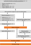 |
Fig. 1. Workflow diagram summarising the main steps of SPRITZ. Orange coloured boxes indicate the outputs of the simulation. |
We now proceed to describe the overall construction of the SPRITZ master catalogue, which is made publicly available2.
2.1. Luminosity functions and galaxy populations
2.1.1. Infrared galaxy populations
We started by extracting simulated galaxies from the Herschel IR LF derived by (Gruppioni et al. 2013, hereafter G13) for different galaxy populations, namely spiral galaxies, starburst (SB), ‘unobscured’ type 1 AGN (AGN1), ‘obscured’ type 2 AGN (AGN2), and two classes of composite systems (SB-AGN and SF-AGN). The latter two represent two galaxy populations without evident AGN activity, two populations dominated by the AGN activity, and two mixed systems. The separation in these six galaxy populations was driven by the observational results presented in Gruppioni et al. (2013) and we maintained the same populations for consistency. We now describe the mentioned galaxy populations, their spectral energy distribution (SED) templates, and their LFs.
Galaxy populations. The population of spiral galaxies contains normal star-forming systems that are dominant in the local Universe but their number density decreases at increasing redshift above z ≃ 1. Spirals range from early bulge-dominated (S0) to late-type disky galaxies (Sdm), such as M 51. Their specific star formation rate (sSFR = SFR/M*) spans the range from log10(sSFR/yr−1) = −10.4 to −8.9 (see later the templates used to derive sSFR).
The SB population contains galaxies with intense episode of star formation: their number increases with redshift and their sSFR varies from log10(sSFR/yr−1) = −8.8 to −8.1. Examples of such objects are M 82, NGC 6090, and Arp 220. Ultra-luminous galaxies (ULIRGs, LIR > 1012 L⊙) are only included in this galaxy population if they do not show any AGN activity.
AGN1 and AGN2 populations contain very luminous AGN that dominate their galaxy energetic compared to their star formation activity. The difference between the two populations resides on the optical to UV part of their spectrum being unobscured (AGN1) or obscured by dust (AGN2). Optically selected quasi-stellar objects (QSO) are examples of AGN1, while optically obscured QSO, such as Mrk 231 and IRAS 19254, are part of the AGN2 population. These two populations, like the previous SB population, show an increase in their numbers with redshift and they dominate the expected galaxy population at z > 2 − 3.
The two composite galaxy populations (SF-AGN and SB-AGN) represent objects that host an AGN that is not the dominant source of energy at any wavelength, apart from a small range in the mid-IR, where the AGN contribution is visible. The G13 authors split them in two sub-populations as they show different redshift evolution and properties. In particular, SF-AGN have a spectrum similar to a spiral galaxy but host a low-luminosity AGN, while SB-AGN resemble SB galaxies hosting an obscured AGN. The SF-AGN dominate the galaxy population at z = 1 − 2, while they are less numerous at lower redshift when spirals galaxies are more common. On the other hand, SB-AGN become more important at increasing redshift (i.e., z > 2), and they can be interpreted as the heavily obscured phase of bright AGN. The star formation of this galaxy population is very high (log10(sSFR/yr−1) ∼ −8.7 in our templates). Following the interpretation of G13 however the system should follow a process of quenching, thereby first becoming a source with a dominant AGN and a lower level of star formation (i.e., AGN1 or AGN2) and then an elliptical galaxy. Seyfert galaxies that show properties similar to star-forming galaxies (García-González et al. 2016), such as Circinus or NGC 1068, are good representatives of SF-AGN, while galaxies such as IRAS 20551, IRAS 22491, and NGC 6240, showing more intense star formation activity, are good examples of SB-AGN.
SED templates. In G13 the Herschel IR LFs were derived by modelling the available optical-to-IR observations with the semi-empirical templates characteristic of each galaxy population. In particular, the templates are taken from the library by (Polletta et al. 2007) with the addition of three SB templates by Rieke et al. (2009) and some templates with a far-IR part modified to better match the Herschel data (see Gruppioni et al. 2010). These adjustments on the original set of templates of (Polletta et al. 2007) were performed by G13 to properly fit the SED of Herschel-detected galaxies. In SPRITZ we consider, for consistency, all 32 SED templates used in G13 (Fig. 2) with each galaxy population having from 3 to 8 SED templates associated with it. The relative importance of each template is dictated by the number of times that template is found to reproduce the photometry of the observed galaxies in G13 at each redshift and IR luminosity.
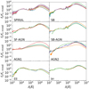 |
Fig. 2. Spectral energy distribution templates used to derive SPRITZ simulated galaxies. Each panel shows templates of a specific galaxy population and all templates are normalised to the flux density at 5500 Å. |
Luminosity functions. Briefly, the shape of the IR LF was assumed to be well represented by the function proposed by Saunders et al. (1990) to describe the 60 μm LF observed with IRAS at low-z as follows:
![Mathematical equation: $$ \begin{aligned} \Phi (L)\mathrm{d}\log _{10}L=\Phi ^{*}\left(\frac{L}{L^{*}}\right)^{(1-\alpha )}\exp \left[-\frac{1}{2\sigma ^{2}}\log ^{2}_{10}\left(1+\frac{L}{L^{*}}\right)\right]\mathrm{d}\log _{10}L ,\end{aligned} $$](/articles/aa/full_html/2021/07/aa39909-20/aa39909-20-eq1.gif) (1)
(1)
where L* and Φ* are the luminosity and the number density at the knee of the LF, where the function changes from behaving as a power law at low luminosities to a Gaussian at high luminosities. The parameter α is the faint-end slope of the LF, while σ regulates the steepness of the bright-end slope. We assumed Φ* and L* to evolve with redshift as
 (2)
(2)
The full list of parameters is shown in Table 1, as derived by G13, while the LF of each galaxy population is shown in Fig. 3. The parameters  and
and  present in the table correspond to the number density and luminosity at the knee of the LF at z = 0. Not all the considered populations show a broken power-law evolution, in these cases the zL, kL, 2, zρ, and kρ, 2 parameters are not given. We note that the evolution of the IR LF at z > 3 is an extrapolation because Herschel observations are generally limited to lower redshift. In particular, we assumed that the characteristic luminosity (L*) remains constant while the galaxy number density decreases as Φ* ∝ (1 + z)kΦ. We explored values for the coefficient kΦ comprised between −1 and −4 to consider the effects of a steep and mild redshift evolution. For AGN1 and AGN2 we applied a different procedure described in the next section because for the AGN1 population the direct use of the Herschel LF creates some discrepancies with far-ultraviolet (FUV) and X-ray observations.
 |
Fig. 3. Infrared LFs used in the SPRITZ simulation to derive simulated galaxies. Each panel shows a different galaxy population, as indicated on the top left. The LFs are shown for different redshifts from 0.1 (solid dark blue line) to 9.6 (solid dark red line) with steps of 0.5. At z > 3 we show the LFs derived assuming kΦ = −1 (see Eq. (2)) for all the populations except for AGN1 and AGN2 for which observations up to z = 5 are available. |
Parameters of the IR LFs used to derive the SPRITZ simulated galaxies, as found by G13 for Herschel galaxies or through the MCMC (for AGN1 and AGN2).
We populated the bright end of the IR LF with galaxies with the SED template showing the highest LIR-to-K ratio, that is those dominated by young stars with respect to the evolved population. When there were multiple templates with similar LIR-to-K ratio for a specific galaxy population, we considered the template with the highest LIR-to-FUV ratio, that is those populated by a relative small fraction of extremely young stars or with a larger amount of dust. We found that this assumption is necessary to avoid an overestimation of the bright end of the K band and FUV LFs and it is applied to objects with log10(LIR/L⊙)≥11.5 for spirals, log10(LIR/L⊙)≥12 for SF-AGN and AGN2, log10(LIR/L⊙)≥12.5 for SB and SB-AGN, and log10(LIR/L⊙)≥11 for AGN1.
2.1.2. Type-1 and type-2 AGN
The large amount of available Herschel data have allowed G13 to derive the LF for different galaxy populations. Achieving this result is not possible when the galaxy sample is limited in number, so a comparison with studies at other wavelengths is generally only possible with the LF of the total galaxy sample. However, in the literature there is a long list of works focussed on studying the LF in the FUV of unobscured AGN-dominated galaxies (i.e., QSO), which dominate the bright end of the FUV LF (e.g., Croom et al. 2009; McGreer et al. 2013; Ross et al. 2013; Akiyama et al. 2018; Schindler et al. 2019). These FUV observations can be used to check the conversion to these wavelengths of the AGN1 IR LF used in SPRITZ.
To perform this comparison we converted the AGN LIR to FUV using the SED templates associated with this galaxy population (Fig. 2). But the AGN contribution to the FUV LF derived from G13 IR LF generally overestimates the observations, particularly at z > 2 and at faint luminosities, where the IR LF was just extrapolated (Fig. A.3). This showed the necessity to improve the AGN LF, but it also ensures that dust-free AGN observed in FUV and not in the IR are expected to be a minority. We therefore decided to improve the AGN1 LF by deriving a new IR LF for this galaxy population using a Monte Carlo Markov chain (MCMC; Foreman-Mackey et al. 2013) applied simultaneously to the FUV and Herschel observations of AGN; the latter are taken for consistency from G13. We considered the same function of the other IR galaxy populations (Eqs. (1) and (2)); but instead of using the extrapolation at z > 3, we exploited as additional constraints the FUV observations, which in the case of AGN1 are available up to z = 5. Following the unification scheme of AGN (Antonucci 1993; Urry & Padovani 1995), AGN1 and AGN2 should represent the same galaxy population observed from different viewing angles. For this reason, we do not expect extreme differences between the AGN1 and AGN2 IR LFs and we find that the Herschel observed LFs derived by G13 are remarkably similar to each other, at least when both AGN populations are available. Given this similarity, we decided to include the observed Herschel LF of AGN1 and AGN2 to our MCMC run. The resulting IR LF describes the Herschel IR observations of AGN1 and AGN2 well, but this LF is also consistent with the FUV QSO observations. The MCMC is described in detail in Appendix A and the best result is listed in Table 1.
2.1.3. Elliptical galaxies
The great majority of elliptical galaxies have low levels of SFR and small amounts of dust (e.g., Knapp et al. 1989; Mazzei & de Zotti 1994; Noeske et al. 2007; McDermid et al. 2015) and their IR luminosity originates, at least in local elliptical galaxies, from dust lanes or diffuse cirrus heated by the radiation field of old stars (e.g., Bertola & Galletta 1978; Goudfrooij & de Jong 1995; Kaviraj et al. 2012; Kokusho et al. 2019). Given their faint IR fluxes, these galaxies are below the detection limit of most Herschel observations and they are not present in the G13 LF study. However, future IR telescopes may be able to detect elliptical galaxies at least at low-z. Therefore, we decided to include elliptical galaxies in the SPRITZ simulation by considering the average LFs derived by Arnouts et al. (2007), Cirasuolo et al. (2007), and Beare et al. (2019) in the K band. We consider these three LFs because they are obtained after removing star-forming systems, which are already included in the Herschel LFs. We extrapolated the K-band LF following Cirasuolo et al. (2007), which goes to higher redshift (z = 2) than the other two works, by maintaining constant the characteristic luminosity and varying the characteristic galaxy density Φ* as ∝(1 + z)−1. This extrapolation is not expected to have a crucial impact on the results because the observed number density of elliptical galaxies at z ∼ 2 is already low (i.e., Φ* = 0.2 × 10⁻³ Mpc−3). The resulting K-band LF at different redshift is shown in Fig. 4.
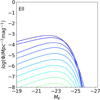 |
Fig. 4. K-band LF used to include simulated elliptical galaxies in the SPRITZ simulation. The LFs are shown for different redshifts from 0.1 (solid dark blue line) to 4.6 (solid green line) with steps of 0.5, using the same colour code of Fig. 3. At z > 2 the LF has been extrapolated, starting from the Cirasuolo et al. (2007)K-band LF. |
As done for the other galaxy populations, we associated with each galaxy extracted from the K-band LF one of the three empirical templates of elliptical galaxies by Polletta et al. (2007, Fig. 2), considering each template with equal probability. The three templates corresponds to galaxies dominated by an old stellar population, but with a different amount of ongoing star formation, that is from log10(sSFR/yr−1) = −12.5 to −11.3, which corresponds to different UV slopes and IR dust bumps. We used these templates to derive physical parameters and to link the K-band LF to the IR LF. This is done through K correction, which is different for each of the three considered templates, resulting in a non-rigid conversion between the K-band LF and the IR LF of elliptical galaxies.
2.1.4. Irregular galaxies
Dwarf irregular galaxies make up another galaxy population that is missing from many Herschel observations, excluding local objects. These galaxies are characterised by a relative low amount of dust, low metallicity and often high sSFR (Hunter et al. 2010; Cigan et al. 2016; Bianchi et al. 2018). They are therefore expected to have bluer optical spectra and fainter LIR, with respect to the other galaxy populations analysed in this work.
We considered the GSMF of star-forming irregular galaxies by Huertas-Company et al. (2016) that is described by a single Schechter function and has been derived for different redshift bins up to z = 3. The faint-end slope α does not show a significant redshift evolution, therefore we assumed a constant value equal to the average weighted mean of the values found at different redshifts (i.e., α = −1.58 ± 0.19). On the other hand, we fitted the redshift evolution of the characteristic stellar mass (log10(M*) = log10( ) and density (
 ) of the GSMF, similar to what has been done by G13 for the other galaxy populations. The fit is shown in Fig. 5 and it results in log
 , kM = 0.06 ± 0.01,
  Mpc−3, and kΦ = −1.22 ± 0.61. The resulting GSMF is shown in Fig. 6.
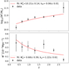 |
Fig. 5. Redshift evolution of the characteristic stellar mass M* (top) and characteristic density Φ* (bottom) of the GSMF of irregular galaxies. Data by Huertas-Company et al. (2016, black dots) and our fit (red solid line) are shown. The latter has been derived with the SCIPY package (Virtanen et al. 2020) and the resulting parameters are reported in each panel. |
 |
Fig. 6. GSMF used to include simulated irregular galaxies in the SPRITZ simulation. The GSMFs are shown for different redshifts from 0.1 (solid dark blue line) to 9.6 (solid dark red line) with steps of 0.5, with the same colour code as in Fig. 3. |
Similar to what has been done for the other galaxy populations, we associated a set of SED templates with simulated irregular galaxies extracted from the mentioned GSMF. In particular, we considered the SED corresponding to the median, the 16% and 84% of the template distribution of irregular galaxies by Bianchi et al. (2018). These three templates are shown in Fig. 2. The median template has been associated with 56% of the simulated galaxies, while the other two to 22% of the irregular galaxy population to match the fraction of galaxies they represent in the observed sample (Bianchi et al. 2018). We made use of these three templates to derive the physical properties and each template is normalised to match the desired LIR.
The LFs or GSMF of the different galaxy populations are sampled from z = 0 to 10 and IR luminosity between log10(LIR/L⊙) = 5 and 15. The number density of each galaxy population in each luminosity–redshift bin is then used to derive the probability to observe each galaxy population in a desired area. This is fundamental for the creation of the simulated catalogues.
2.2. Physical properties of simulated galaxies
In this section we describe the method used to retrieve the various physical parameters associated with each LIR − z bin of the master catalogue. For all templates, the total LIR is derived directly integrating the templates between 8 and 1000 μm. In order to derive the other main physical parameters such as stellar mass and colour excess for all simulated galaxies, we applied the Multi-wavelength Analysis of Galaxy Physical Properties (MAGPHYS, da Cunha et al. 2008) package, or the software SED3FIT (Berta et al. 2013) based on MAGPHYS when an AGN contribution is present to the set of templates associated with each galaxy population. This SED fitting procedure serves to infer the physical properties associated with each SED template because this information is not available a priori because of the empirical nature of the templates described in Sect. 2.1.1. To perform the fit, we created a large set of simulated observations of custom filters spanning from FUV to far-IR wavelengths and assigning S/N of 10 to each of them. For the AGN component, we considered a library with smooth (Fritz et al. 2006; Feltre et al. 2012) and clumpy tori (Nenkova et al. 2008a,b), as explained in more detail in the next section. The analysis of the AGN component is necessary to disentangle the contribution of the AGN and star formation to the total IR-luminosity and to take into account the contamination of the AGN when deriving the stellar mass. In the fits by both MAGPHYS and SED3FIT we considered Bruzual & Charlot (2003) stellar templates with Chabrier (2003) IMF. For all considered empirical templates we retrieved the best fit value of the different physical parameters estimated by SED3FIT or MAGPHYS, as well as the 2.5%, 16%, 84%, and 97.5% percentile when available3. When assigning a physical property to a simulated galaxy, we randomised each parameter value following the corresponding probability distribution to take into account the uncertainties on the SED fitting procedure. When a probability distribution is not available, we assumed a Gaussian distribution centred to the best value and an arbitrary σ = 0.3 dex. In the master catalogue we considered only the median value of each parameter, as derived for each galaxy population and LIR − z bin.
As new stars may be surrounded by dust, an estimation of the total amount of star formation requires accounting for both the direct light emitted by young stars, for example looking at UV wavelengths, and for the amount of light absorbed by dust, looking at the reprocessed light at IR wavelengths. In our case, we considered the contribution of the star formation to the IR luminosity to estimate the obscured star formation rate (SFR) and the observed rest-frame UV at 1600 Å, that is the luminosity at 1600 Å computed on the template not corrected for dust attenuation, to estimate the unobscured component of SFR associated with each template. These two properties can be estimated following Kennicutt (1998a,b):
![Mathematical equation: $$ \begin{aligned}&\mathrm{SFR}_{\rm UV}[M_{\odot }\,\mathrm{yr}^{-1}]=f_{\rm IMF}\,4.5\times 10^{-44}\,L_{\nu ,1600\,\upmu \mathrm{m}}[\mathrm{erg\,s}^{-1}],\nonumber \\&\mathrm{SFR}_{\rm IR}[M_{\odot }\,\mathrm{yr}^{-1}]=f_{\rm IMF}\frac{L_{3{-}1000\,\upmu \mathrm{m}}[L_{\odot }]}{5.8\times 10^9}, \end{aligned} $$](/articles/aa/full_html/2021/07/aa39909-20/aa39909-20-eq23.gif) (3)
(3)
where fIMF = 0.63 (Murphy et al. 2011) represents the conversion from a Salpeter (1955) to Chabrier IMF. The total SFR is the sum of the two components, SFRtot = SFRUV + SFRIR.
For each simulated galaxy we derived the gas–phase metallicity from the mass–metallicity relation by Wuyts et al. (2014) as
![Mathematical equation: $$ \begin{aligned}&12 + \mathrm{log}_{10}(\mathrm{O/H}) = Z_{0} + \mathrm{log}_{10} [1-\exp (-(M^{*}/M_{0})^{\gamma } ], \nonumber \\ &\mathrm{log}_{10}(M_{0}/M_{\odot }) = (8.86 \pm 0.05) + (2.92 \pm 0.16)\,\mathrm{log}_{10}(1 + z), \end{aligned} $$](/articles/aa/full_html/2021/07/aa39909-20/aa39909-20-eq24.gif) (4)
(4)
where the power-law slope at low metallicity is γ = 0.40 and the asymptotic metallicity is Z0 = 8.69. This mass–metallicity relation is in overall agreement with the relation proposed by Mannucci et al. (2010, 2011), at least among intermediate and massive galaxies (see Wuyts et al. 2014). We did not consider the metallicity derived from the SED fitting, as otherwise the metallicity would be fixed to a specific value independently by the stellar mass.
2.2.1. AGN torus library
We made use of the SED3FIT code to derive the AGN contribution of all the galaxies with an AGN component using two distinct torus libraries. The first library consists of the smooth torus models presented by Fritz et al. (2006) and Feltre et al. (2012). The second is the library of clumpy torus models presented in Nenkova et al. (2008a,b).
In particular, we considered smooth torus models with an outer to inner radii ratio Rout/Rin = 10 and 30. We limited the fit to models with Rout/Rin ≤ 30, as suggested by previous works and observations (e.g., Jaffe et al. 2004; Netzer et al. 2007; Hatziminaoglou et al. 2008; Pozzi et al. 2010; Mullaney et al. 2011; García-Burillo et al. 2019). The considered torus models have torus amplitude angle Θ, defined as the angular region occupied by the torus dust, from 60° to 140°. The dust density distribution of the torus varies along the radial and vertical directions, as described in polar coordinates ρ(r, θ) = A rβe−γ cos(θ). The spectrum of the central engine is instead modelled with a broken power law (Eq. (1) of Feltre et al. 2012) with spectral index α, λL(λ) ∝ λα, at 0.125 < λ < 10.0 μm fixed to α = −0.5. Finally, the equatorial optical depth at 9.7 μm (τ9.7) is between 0.1 and 10 and we considered viewing angles (ϕ) between 0° and 90°.
For the clumpy torus models we considered templates with an outer to inner radii ratio Rout/Rin = 10 and 30, as done for the smooth torus models. The density profile of the dust clumps is described radially by a power law and vertically by an exponential profile ρ(r, θ) ∝ r−q e−|θ/σ|m with m = 2 for smooth boundaries. We considered models with q values between 0 and 3 and with torus width σ, that is Gaussian distribution of the clouds, between 20° and 70°. The selected models are also parametrised in terms of the average number of clouds along a radial direction on the equatorial plane, comprised between 1 and 15. Ramos Almeida et al. (2009) find a median number of clouds of 10 using mid-IR observations of Seyfert galaxies, but larger values are necessary to include very obscured AGN in the SPRITZ simulation. For a given combination of parameters, all the clouds have the same optical depth τv and we considered values between 10 and 200.
The entire list of the model parameters is shown in Table 2 for both template families. In Fig. 7, we compare the stellar mass, hydrogen column density, and X-ray luminosity (see Sect. 2.2.2 for its derivation) obtained with the two torus libraries after scaling all the templates to have LIR = 1011 L⊙. These three derived quantities generally agree even if with some scatter. The major differences for the stellar mass correspond to AGN-dominated systems, that is AGN1 and AGN2. These discrepancies are not surprising for AGN1, as their stellar mass is difficult to estimate because the AGN light dominates even at optical wavelengths. The maximum value of the hydrogen column density of our library of smooth torus is log10(NH/cm−2) ∼ 23.6. The inclusion of the clumpy torus model is therefore fundamental to simulate heavily dust-obscured AGN. The hydrogen column densities derived considering clumpy torus models, in fact, are generally larger than those derived with smooth torus models. The two torus models agree on the intrinsic X-ray luminosity of the brightest objects at fixed IR luminosity, while for the faintest objects the clumpy torus models predict higher X-ray luminosities than the smooth models. When comparing the two torus libraries, it is important to mention that the intrinsic X-ray luminosity depends not only on the hydrogen column density, but also on the AGN-host galaxy decomposition. As shown in the same figure, the intrinsic X-ray luminosities derived with the two torus models differ more for composite systems than for AGN-dominated objects.
 |
Fig. 7. Comparison between the stellar mass (left), hydrogen column density (centre), and intrinsic X-ray luminosity (right) derived using SED3FIT with the clumpy and smooth torus library. All considered SED templates are scaled to have LIR = 1011 L⊙. Symbols indicate different galaxy populations: SF-AGN (dark-green circles), SB-AGN (orange squares), AGN type-1 (blue triangles), and AGN type-2 (magenta stars). In the central panel, empty symbols and arrows represent the upper limits to NH for the objects for which NH = 0 with one torus library, but not with the other torus library. These points are artificially set to log10(NH/cm−2 = −20.5 for visual purposes. We do not show objects for which NH = 0 using both torus libraries; this is comprised of three AGN1 templates and one SF-AGN template. The vertical dashed grey line indicates the maximum values of NH of the smooth torus library. Error bars indicate the 16% and 84% percentiles and, in the right panel, the scatter of 0.33 dex in the relation to derive X-ray luminosity (Asmus et al. 2015). The black dotted line in each panel indicates the identity line. |
Parameters considered for smooth torus models (left) and clumpy torus models (right), as described in Sect. 2.2.1. Fritz et al. (2006), Feltre et al. (2012), and Nenkova et al. (2008a,b) provide further details.
In the SPRITZ simulation we randomly associated a smooth torus model with half of the objects hosting an AGN and a clumpy torus model with the remaining half, but we include in the uncertainties the results derived including separately only one of the two torus models. For more details on the SED fitting code, we refer to Berta et al. (2013); for the torus models, we refer to Feltre et al. (2012), Fritz et al. (2006), and Nenkova et al. (2008a,b).
2.2.2. X-ray luminosity
From the AGN decomposition performed with SED3FIT we retrieved, for each simulated galaxy, the line-of-sight optical depth at 9.7 μm (τ9.7) and the hydrogen column density associated with the torus model. The smooth torus models have values of the hydrogen optical depth below log10(NH/cm−2) < 23.6 and it is therefore not possible to reach the Compton-thick regime (i.e., log10(NH/cm−2) > 24) using such models. For the clumpy torus models we derived the hydrogen column density of the torus from the optical depth in the V band (τV) of the torus, which is among the input parameters of the model, considering that NH = 1.8 × 10²¹ 1.086 τV cm−2 (Predehl & Schmitt 1995). The intrinsic hard X-ray luminosity, as derived at 2–10 keV, is estimated from the luminosity at 12 μm associated with the AGN component, using the relation derived by Asmus et al. (2015), considering a sample of IR and X-ray selected AGN,
 (5)
(5)
As mentioned in the same paper, this relation has been tested for AGN with X-ray luminosity below log10(L2−10 keV/ergs−1) = 45 and a possible flattening of the relation could be present at higher luminosity. At higher X-ray luminosity, we considered the bolometric correction derived by Duras et al. (2020) using a sample of X-ray selected AGN. The bolometric correction is described as a function of the AGN bolometric luminosity for bright AGN (i.e.,  ) and it is constant otherwise. We derived the AGN bolometric luminosity from the SED3FIT fit. The comparison between the two intrinsic X-ray luminosity values for all AGN in SPRITZ is shown in Fig. 8 for both clumpy and smooth torus. The X-ray luminosity derived using the bolometric correction is larger than the other value for the majority of galaxies, except for the brightest AGN. As previously mentioned, the bolometric correction derived by Duras et al. (2020) is a function of the bolometric luminosity for the brightest AGN, while it is constant for fainter AGN. The two X-ray luminosities are very similar for the AGN1 and AGN2 populations, while they differ for the composite systems, particularly for the SB-AGN population described by a smooth torus. Differences in the two approaches may arise from the different samples of AGN considered to derive the two relations, as this may suggest the similarity between the most X-ray luminous AGN (AGN1 and AGN2). On the other hand, it is necessary to consider that there are also uncertainties on the AGN-host galaxy decomposition performed in this work.
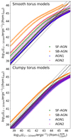 |
Fig. 8. Comparison between the X-ray luminosity obtained from the luminosity at 12 μm (Asmus et al. 2015) and the X-ray luminosity obtained from the AGN bolometric luminosity and assuming the correction by Duras et al. (2020). The comparison is shown separately for the smooth (top) and clumpy torus models (bottom). The different colours indicate the galaxy populations with an AGN component (see legend). The X-ray luminosities are compared before applying any dispersion and are shown for the smooth (top) and clumpy torus models (bottom). The dashed black line indicates the identity line while the dotted lines show the 1σ combined dispersion of the two relations. |
In the SPRITZ simulation, we assigned to each simulated galaxy the X-ray luminosity derived from the luminosity at 12 μm. This choice is motivated by the presence of IR-selected AGN in the sample used by Asmus et al. (2015) because the main aim of this work is to create realistic IR simulated galaxies. In addition, the peak of the AGN emission at 12 μm should be less affected by the used torus model than the bolometric AGN luminosity. Last, but not least, the X-ray luminosity derived from the L12 μm shows a better agreement with the observed X-ray LF than the X-ray luminosity derived with the bolometric correction (see Sect. 4).
We randomly scatter the X-ray luminosity of each simulated galaxy around the value derived from the relation by Asmus et al. (2015), considering a Gaussian distribution with σ = 0.33, which corresponds to the uncertainty derived in the same work.
After deriving the intrinsic X-ray luminosity, we retrieved the observed luminosity L2 − 10 keV, obs considering the description by Lusso et al. (2010) as follows:
 (6)
(6)
where A is the normalisation derived to match the intrinsic hard X-ray luminosity; Ecut is the high-energy cut-off of the primary AGN power-law component, assumed to be 200 keV (Gilli et al. 2007); and σE is the effective photoelectric absorption cross-section for hydrogen atoms (Table 2 from Morrison & McCammon 1983). Finally, Γ is the X-ray slope and it assumed to be equal to 2 in the soft X-ray (0.5–2 keV) and equal to 1.7 in the hard X-ray (2–10 keV). The same X-ray SED (Lusso et al. 2010) is considered to retrieve the soft and hard X-ray fluxes. In the SPRITZ simulation, when deriving the observed X-ray luminosity we applied the scatter associated with both the intrinsic luminosity and the hydrogen column density.
To summarise, using the different empirical relation mentioned above, we assigned to each simulated galaxy with an AGN component an intrinsic and observed luminosity at 2–10 keV, as well as the expected flux in the soft and hard X-ray. The simulation does not include any X-ray emission arising from the host galaxy.
2.2.3. Radio luminosity
We derived the expected radio luminosity due to the star formation activity at 1.4 GHz for each simulated galaxy by considering the redshift evolution of the logarithmic ratio of the 1.4 GHz and total IR luminosity by Delhaize et al. (2017). In particular, we considered the updated version of this relation, as derived after removing possible radio AGN contribution by Delvecchio et al. (2018) as follows:
 (7)
(7)
In the IR luminosity we included only the component due to star formation.
We also included the contribution of radio-loud AGN by combining the estimated fraction of radio-loud AGN by Best et al. (2005) and the pure-luminosity evolution of the 1.4 GHz LF of AGN by Smolčić et al. (2017). In particular, Best et al. (2005) find that the local fraction of radio-loud AGN above a certain radio luminosity at 1.4 GHz depends on stellar mass as
![Mathematical equation: $$ \begin{aligned} f_{\rm RL}=f_{0} \left( \frac{M^{*}}{10^{11}\,M_{\odot }} \right)^{\alpha }\left[\left(\frac{L}{L_{*}}\right)^{\beta }+\left(\frac{L}{L_{*}}\right)^{\gamma }\right]^{-1} ,\end{aligned} $$](/articles/aa/full_html/2021/07/aa39909-20/aa39909-20-eq29.gif) (8)
(8)
where f0 = 0.0055 ± 0.0004 is the normalisation factor, α = 2.5 ± 0.2 accounts for the scaling between the fraction of radio-loud AGN and stellar mass, whereas L*, β and γ are the knee, the faint, and the bright-end slope of the LF, respectively. The local LF found by Best et al. (2005) is generally lower than those found by other authors (Ceraj et al. 2018); in this work we decided to consider the results by Mauch & Sadler (2007), that is L* = 1024.59 W Hz−1, β = 1.27 and γ = 0.49. The same local radio-AGN LF are also considered by Smolčić et al. (2017), from which we derived its pure-luminosity evolution with redshift as
![Mathematical equation: $$ \begin{aligned} \Phi (L,z,\alpha _{\rm L},\beta _{\rm L})=\Phi _{0} \left[ \frac{L}{(1+z)^{\alpha _{\rm L}+z\,\beta _{\rm L}}} \right],\end{aligned} $$](/articles/aa/full_html/2021/07/aa39909-20/aa39909-20-eq30.gif) (9)
(9)
where αL = 2.88 ± 0.82, βL = −0.84 ± 0.34, and Φ0 is the local radio-AGN LF. As also stated in Smolčić et al. (2017), considering the pure-density evolution instead of the pure-luminosity evolution gives similar results. We then combined Eqs. (8) and (9) to estimate the probability for a simulated galaxy in SPRITZ to be a radio-loud AGN with a specific 1.4 GHz luminosity, starting from its stellar mass and redshift. We considered a single population of radio-loud AGN, without separating for their accretion mechanisms (Best et al. 2005; Tasse et al. 2008). These different radio-loud AGN populations may be considered in future studies.
We also derived for each simulated galaxy the expected luminosity due to the star formation activity at 150 MHz, following the empirical relation by Gürkan et al. (2018):
![Mathematical equation: $$ \begin{aligned} \begin{split} L&_{\rm 150\,MHz}[\mathrm{W\,Hz}^{-1}]= \\&\Bigg \{ \begin{array}{lr} L_{\rm C}\, \mathrm{SFR}^{\beta _{\rm low}}\left(\frac{M_{*}}{10^{10}\,M_{\odot }}\right)^{\gamma },&\mathrm{if} \,\mathrm{SFR} \le \mathrm{SFR}_{\rm break}\\ L_{\rm C}\,\mathrm{SFR}^{\beta _{\rm high}}\left(\frac{M_{*}}{10^{10}\,M_{\odot }}\right)^{\gamma }\mathrm{SFR}_{\rm break}^{\beta _{\rm low}-\beta _{\rm high}},&\mathrm{if}\,\mathrm{SFR} > \mathrm{SFR}_{\rm break} \\ \end{array} \end{split}\!\!\!,\end{aligned} $$](/articles/aa/full_html/2021/07/aa39909-20/aa39909-20-eq31.gif) (10)
(10)
where the normalisation is log10(LC/W Hz−1) = 22.02 ± 0.02, the slopes are βlow = 0.52 ± 0.03, βhigh = 1.01 ± 0.02 and γ = 0.44 ± 0.01, and the position of the break is log10(SFRbreak [M⊙ yr−1]) = 0.01 ± 0.01.
2.3. Emission features
To investigate the spectroscopic capability of future telescopes, we included in the SPRITZ simulation a large set of emission features mainly, but not only, in the IR wavelength range.
We derived the relative contribution of AGN and star-formation for each galaxy template from the AGN-galaxy decomposition obtained by SED3FIT. We then used several empirical relations between the luminosity of IR emission lines and the IR luminosity, either total or decomposed into SF and AGN contribution. In particular, we considered the empirical relations derived by Gruppioni et al. (2016), Bonato et al. (2019), and Mordini et al. (in prep.). For each line, Gruppioni et al. (2016) and Mordini et al. (in prep.) derived two relations, for AGN dominated systems and for galaxies in which the AGN is a minor component. In the SPRITZ simulation this separation is applied to galaxies above or below fAGN = 40%, where fAGN is the AGN fraction contributing to the light emitted between 5 and 50 μm. The full list of IR emission features included in the SPRITZ simulation is listed in Table 3 together with the corresponding reference. In Bonato et al. (2019), there are also relations linking the LIR to the CO molecular lines, which we also included. All line luminosities, including the luminosity of the different PAH features that are already present in the SED templates associated with each simulated galaxies, are listed separately in the catalogue for quick reference, for example to estimate the expected line luminosity of galaxies without fitting the corresponding spectra. In Fig. 9 we show as an example the comparison of the line luminosities of the PAH at 3.3 μm, [Ne V] 14.32 μm, and [O I] 63.18 μm lines, as derived from the corresponding relations.
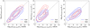 |
Fig. 9. Comparison between the line luminosities derived using the relation by Bonato et al. (2019, B19, x-axis) with those derived with the relations by Gruppioni et al. (2016, blue solid lines) and Mordini et al. (in prep., red dashed lines). The contour lines indicate the 68%, 95%, and 99.7% percentiles of the distribution. The three panels show three different lines: PAH at 3.3 μm (left), [Ne V] 14.32 μm (centre), and [O I] 63.18 μm (right). The relations may be different for AGN and star-forming dominated systems, as explained in the text. |
IR emission features considered in the catalogue with the respective references: B19: Bonato et al. (2019), G16: Gruppioni et al. (2016), and M20: Mordini et al. (in prep.).
In addition, we included in the SPRITZ simulation a set of recombination lines of the atomic hydrogen, from the Balmer to the Humphreys series. The Hα emission line was derived assuming the relation with the SFR by Kennicutt (1998b). All the other lines were then derived by considering the line intensity ratio by Hummer & Storey (1987) and Osterbrock & Ferland (2006) for the case B recombination with electron temperature Te = 10 000 K in the low density limit (i.e., electron density Ne = 100 − 10 000 cm−3). Table 4 contains the complete list of the atomic hydrogen lines considered in the simulation.
Recombination lines of the atomic hydrogen included in the SPRITZ simulation with the corresponding vacuum wavelengths (Lang 1999; Morton 2000).
We also included some of the main nebular emission lines at optical and near-IR wavelengths (Table 5). In particular, using the relation by Kennicutt (1998b) we derived the luminosity of the [O II] doublet at 3727/3729 Å from the SFR as
![Mathematical equation: $$ \begin{aligned} L([{\text{O}}{\small {{\text{II}}}}])\,[\mathrm{erg\,s}^{-1}] = \frac{\mathrm{SFR} [M_{\odot }\,\mathrm{yr}^{-1}]}{(1.4\pm 0.4)\times 10^{-41}} \cdot \end{aligned} $$](/articles/aa/full_html/2021/07/aa39909-20/aa39909-20-eq32.gif) (11)
(11)
Optical nebular emission lines included in the SPRITZ simulation for both star-forming systems and AGN.
To derive the luminosity of the [N II] line at 6584 Å, we applied the relation between metallicity and the [N II]/Hα by Pettini & Pagel (2004) given by
![Mathematical equation: $$ \begin{aligned} \mathrm{log}_{10}\left( \frac{[{\text{N}}{\small {{\text{ II}}}}]}{\mathrm{H}_{\alpha }} \right)=\frac{12+\mathrm{log}_{10}(\mathrm{O/H})-8.90}{0.57}, \end{aligned} $$](/articles/aa/full_html/2021/07/aa39909-20/aa39909-20-eq33.gif) (12)
(12)
considering a 1σ scatter of 0.18 dex. From the metallicity we also derived the [Ne III] nebular emission line at 3869 Å, using the relation derived at z ∼ 0.8 by Jones et al. (2015), which is also consistent with local observations, written as
![Mathematical equation: $$ \begin{aligned} \mathrm{log}_{10} \left( \frac{[{\text{ Ne}}{\small {{\text{ III}}}}]}{[{\text{ O}}{\small {{\text{ II}}}}]} \right)=16.8974-2.1588\,(12+\mathrm{log}_{10}(\mathrm{O/H})) .\end{aligned} $$](/articles/aa/full_html/2021/07/aa39909-20/aa39909-20-eq34.gif) (13)
(13)
For this relation we considered an intrinsic scatter of σ = 0.22 dex (Jones et al. 2015). We also included the expected luminosity of the [N II] line at 6548 Å considering the theoretical value of one-third (Osterbrock & Ferland 2006). The luminosity of the [O III] forbidden line at 5007 Å is derived considering the relation derived by Kewley et al. (2013a) for galaxies at z < 3. This relation relates the [O III]/Hβ ratio to the [N II]/Hα ratio and includes the evolution with redshift
![Mathematical equation: $$ \begin{aligned} \mathrm{log}_{10} \left( \frac{[{\text{ O}}{\small {{\text{ III}}}}]}{H_{\beta }} \right) =1.1+0.3\,{z} +\frac{0.61}{\mathrm{log}_{10}([{\text{ N}}{\small {{\text{ II}}}}]/\mathrm{H}_{\alpha })+0.08-0.1833\,{z}} \cdot \end{aligned} $$](/articles/aa/full_html/2021/07/aa39909-20/aa39909-20-eq35.gif) (14)
(14)
The luminosity of the [O III] forbidden line at 4959 Å is then assumed to follow the theoretical value and to be one-third of the luminosity of the [O III] at 5007 Å (Osterbrock & Ferland 2006). The luminosity of the [S II] doublet at 6717/6731 Å is derived considering the empirical relation between the metallicity, the [N II], and the Hα lines by Dopita et al. (2016) as follows:
![Mathematical equation: $$ \begin{aligned} 12+\mathrm{log}_{10}(\mathrm{O/H})=8.77+\mathrm{log}_{10} \left( \frac{[{\text{ N}}{\small {{\text{ II}}}}]}{[{\text{ S}}{\small {{\text{ II}}}}]} \right) + 0.264\,\mathrm{log}_{10} \left( \frac{[{\text{ N}}{\small {{\text{ II}}}}]}{\mathrm{H}_{\alpha }} \right) .\end{aligned} $$](/articles/aa/full_html/2021/07/aa39909-20/aa39909-20-eq36.gif) (15)
(15)
To separate the contribution of the two [S II] doublet lines, whose ratio depends on the electron density (ne), we first derived the expected electron density from the specific SFR and the stellar mass, following the empirical relation found by Kashino et al. (2019):
 (16)
(16)
We then used the electron density to derive the ratio of the [S II] doublet lines, assuming an electron temperature of 104 K and the empirical relation by Proxauf et al. (2014) as follows:
 (17)
(17)
where R is the ratio of the 6716 Å–6731 Å [S II] line flux.
As similar empirical relations are not available for AGN, we considered predictions from photo-ionisation calculations for the same lines listed in Tables 4 and 5. In particular, we incorporated the contribution from the narrow-line gas emitting regions (NLR) of AGN to the line emission of AGN-SB, AGN-SF, AGN1, and AGN2. The emission from the broad-line gas emitting (BLR) is not included in the current version of SPRITZ and will be the subject of future works. This only impacts the line emission of the permitted lines in AGN1, whose emission should be considered as a lower limit at present.
The model describing the NLR emission is that from Feltre et al. (2016), which is based on the phoionisation code CLOUDY (v13.03, Ferland et al. 2013). In particular, to derive the desired line luminosities, we considered an ionisation parameter at the Strömgren radius between log10(US) = − 1.5 and −3.5, sub- and super-solar metallicity (0.008, 0.017, 0.03), a dust-to-metal ratio of 0.3, a UV spectral index α = −1.4, and an internal micro-turbulence velocity v = 100 km s−1 (see Mignoli et al. 2019). The hydrogen number density is assumed to be 103 cm−3 for type-1 AGN, which are defined as AGN with hydrogen column density log10(NH/cm−2) < 22. This division is obvious for our AGN1 and AGN2 populations and it is mainly necessary to separate SF-AGN and SB-AGN into obscured and non-obscured AGN.
We applied attenuation from dust to all the lines assuming the Charlot & Fall (2000) cloud model to be consistent with the dust model used in MAGPHYS. In particular, the dust attenuation has a diffuse component, describing the interstellar medium (ISM), and a component concentrated around young stars, representing their birth clouds. As emission lines are predominantly generated by young stellar systems, we assumed that they are affected by both components. The two components of the optical depth depend differently on wavelength: the ISM component is  , while the birth clouds component is
  . Both the average V-band optical depth and the fraction of the ISM contribution to it are derived from the SED fit performed with MAGPHYS or SED3FIT. For each line, we include the scatter associated with each considered relation, as written in the respective papers, or a generic scatter of 0.1 dex when the relative papers do not quote the value. Future releases may include additional lines as well as emissions from the BLR.
3. Creation of the simulated catalogues
As described in the previous sections, we derived a master catalogue starting from the observed LFs and GSMF of the different galaxy populations. This catalogue contains the number density of each galaxy population in specific LIR − z bins, as well as the median values of the physical parameters associated with the population. From the master catalogue, it is possible to derive simulated catalogues corresponding to current and future spectro-photometric surveys once their area and depth are known.
In particular, from the area of the survey we derived the volume of the Universe corresponding to each redshift bin considered in the master catalogue and then the expected number of galaxies N0(z, LIR) for each galaxy population at the various redshift. To include the variance on the simulated catalogues, we considered the Poisson errors associated with N0(z, LIR) and we generated a number of simulated galaxies equal to  . To each simulated galaxy we assigned random values of IR luminosity and redshift, considering a flat probability distribution inside the corresponding LIR − z bin. We then assigned the various physical properties mentioned in the previous sections, by randomly extracting a value following the corresponding probability distribution function. To summarise, we ended up with a series of simulated galaxies corresponding to different galaxy populations and their number is derived from the corresponding LFs, or GSMF for irregular galaxies, and depends on the area of the simulated survey. It is now necessary to verify which galaxy is expected to be detected in the desired survey by retrieving a set of simulated fluxes and spectra to compare with the spectro-photometric depth of the survey of interest at specific wavelengths. The derivation of simulated fluxes and spectra is described in the following sections.
3.1. Simulated fluxes
To retrieve the expected flux in different bands for each simulated galaxy, we convolved the SED templates associated with each galaxy population with different filter throughputs. In particular, we included a set of absolute magnitudes in standard filters: NUV (GALEX, Zamojski et al. 2007), u, r (Sloan Digital Sky Survey, Zehavi et al. 2011), B, V (SUBARU SUPRIME-CAM, Miyazaki et al. 2002), J (UKIRT/WFCAM, Casali et al. 2007), and Ks (WIRCam, Puget et al. 2004). We also derived for each simulated galaxy the expected flux for some past, current, and future facilities among which the JWST, Euclid (Laureijs et al. 2010), Spitzer (Werner et al. 2004), the Sloan Digital Sky Survey (SDSS; Gunn et al. 1998), the United Kingdom Infrared Telescope, the Hubble Space Telescope (HST), Herschel, the SCUBA-2 instrument on the James Clerk Maxwell Telescope (Holland et al. 2013), the AKARI telescope (Murakami et al. 2007), the Wide-field Infrared Survey Explorer (Wright et al. 2010), the European Extremely Large Telescope (ELT; Gilmozzi & Spyromilio 2008), the Vera Rubin Observatory (LSST; Ivezic et al. 2008), and OST. The complete list of filters included in the simulation with the corresponding central wavelengths and references is shown in Appendix B. Additional filters may be included in future updates. In addition, considering the hydrogen column density derived with SED3FIT for each template and the X-ray SED described in Sect. 2.1.1, we retrieved the expected flux in the soft 0.5–2 keV and hard 2–10 keV X-ray bands. Additional filters may be considered in future updates.
To simulate a specific survey we then considered the flux in the filter of interest and we derived the flux error considering the desired observational depth. We applied a random scatter to each flux equal to the desired observational depth.
3.2. Simulated IR low-resolution spectra
In the SPRITZ simulation we included synthetic spectra derived considering the wavelength coverage, resolution and the sensitivity expected for the low-resolution spectra for the JWST Mid-Infrared Instrument (MIRI, Kendrew et al. 2015; Rieke et al. 2015; Wright et al. 2015) and the low-resolution Origins Survey Spectrometer (OSS; Bradford et al. 2018) planned for OST (Table 6). Briefly, JWST/MIRI-LR covers between 5 and 12 μm with resolving power ranging from ∼40 at 5μm to ∼160 at 10μm. The OST/OSS is expected to cover between 25 and 590 μm with spectral resolution R = 300 and wide-field survey capability. Additional spectrographs, like other JWST spectroscopic modes, may be considered in future update.
Wavelength coverage and spectral resolution of the three spectrographs considered in SPRITZ.
For consistency with the photometric predictions, we started from the same set of empirical templates used in the rest of the simulation, that is 35 templates from Polletta et al. (2007), Rieke et al. (2009) and Bianchi et al. (2018). These templates are similar to the SB templates by Brandl et al. (2006) and Hernán-Caballero & Hatziminaoglou (2011) in the overlapping galaxy population. The SB-AGN templates show a very deep 9.7 μm silicate absorption feature that is not present in other works. Therefore, for this galaxy population we considered a combination of the continuum of the SED template used for photometry and the features present in the Seyfert2 template by Hernán-Caballero & Hatziminaoglou (2011). When necessary, we converted all the templates to vacuum wavelengths4 (Morton 2000).
We added several nebular emission lines to the spectra considering the expected line luminosity derived using different empirical and theoretical predictions, as explained previously in Sect. 2.3. We included all the nebular emission lines, but we did not insert PAH features because they are already present in the templates. Since the template spectra included in SPRITZ are empirical, some of the optical nebular lines are already included. When this happens, we removed the line from the spectra by linearly interpolating the continuum around the line before adding the new nebular emission line with the desired luminosity. In other words, we assumed a flat continuum around the nebular emission lines, which are generally very narrow. This assumption is not expected to impact the results much because we aim to simulate low-resolution spectra; however, when necessary, the use of the MAGPHYS or SED3FIT template can be considered to avoid this issue. For the component due to star formation, we derived the expected gas velocity dispersion from the stellar mass to take into account the broadening of the nebular emission lines (Bezanson et al. 2018) as follows:
 (18)
(18)
For nebular emission lines of AGN we assumed full width half maximum (FWHM) between 500 and 800 km s−1. We assumed the central wavelengths from Lang (1997) and we converted it to vacuum wavelength (Morton 2000).
For each simulated galaxy we shifted the corresponding empirical template to the assigned redshift and we applied the wavelength resolution of the desired spectrograph, that is JWST/MIRI-LR or OSS/OST. An example of a JWST/MIRI low-resolution spectra is reported in Fig. 10, where we show the simulated spectra of a SB-AGN galaxy at z = 2.88, considering the slit observational mode. We considered an exposure time of 10 h, reaching a 5σ continuum depth of 0.18 and 3.56 μJy at 5 and 12 μm, respectively. The example shows the inclusion of bright hydrogen lines (i.e., Brα, Brβ, and Brγ) with the contribution of AGN and star formation. Fainter lines, such as Brδ and Br9, were included but are below the continuum level. We considered the spectral resolving power and continuum sensitivity reported in Glasse et al. (2015).
 |
Fig. 10. Example of a low-resolution JWST/MIRI spectra of a SB-AGN galaxy at z = 2.88. At the top the rest-frame wavelengths are shown; on the bottom the observed wavelengths are shown. The original spectrum (solid black line), the spectrum after the addition of nebular lines (dashed red line), and the spectrum after the application of the spectral resolution and noise (dotted green line) are shown. On the top, short vertical dotted lines indicate the wavelength position of the nebular emission lines included despite their S/N. |
3.3. Light cone creation
In order to simulate galaxies ‘realistically’ distributed in the sky, we made use of the algorithm by Soneira & Peebles (1978) to distribute galaxies following a two-point correlation function with a specific power law. The algorithm starts by generating a first layer consisting of η random points within a circle of radius R. The second layer consists of η points, extracted randomly within a circle of radius R/λ centred on each point of the previous level. This procedure is repeated for each level, up to a specific L level, each time reducing the size of the circle by a factor of λ and using the points of each level to generate the points of the next one. In this way, the nth level has ηn points in total and each group of η points is generated randomly in a circle, which is centred on the ηn − 1 points of the previous level and has a radius of R/λn. We repeat this procedure for different redshift bins, from z = 0 to 10, and we included additional scatter among z bins to avoid sharp features.
The two-point correlation function can be roughly described as a power law in real space ξ = (r/r0)−γ and, using the approximation by Limber (1953), the angular correlation function is w(θ) = Awθ1 − γ. In our simulation we assumed a power-law slope for the angular correlation function δ = γ − 1 = 0.7, as suggested by observations (e.g., Wang et al. 2013). In the algorithm by Soneira & Peebles (1978), the power-law slope of the angular correlation function is related to the η and λ parameters as
 (19)
(19)
where M is the number of dimensions and R, L, and λ are in arc-second. We therefore assumed η = 6 and λ = 4. The starting radius R is chosen to cover the desired survey area and the parameter L is fine-tuned to obtained a number of positions equal or larger than the number of simulated galaxies.
The clustering of galaxies shows a dependence with stellar mass because more massive galaxies tend to live in denser environments (e.g., Li et al. 2006; Meneux et al. 2008; Wake et al. 2011; Marulli et al. 2013). To reproduce this effect we derived the dependence of the spatial correlation length r0 on stellar mass limit using data from Wake et al. (2011) and Hatfield et al. (2016), which consider the same power-law slope considered in this work. Literature works have shown that r0 has little or no evolution with redshift (Béthermin et al. 2015; Schreiber et al. 2015), therefore we only considered its dependence on the stellar-mass limit. Briefly, we describe the r0 dependence on stellar-mass limit as a broken power law as follows:
 (20)
(20)
where the stellar mass break equal to log . The resulting best fit corresponds to a low-mass slope of kM, 1 = 0.0959 ± 0.0003 and a high-mass slope of kM, 2 = 0.181 ± 0.006. From the spatial correlation length r0, it is then possible to derive the normalisation of the angular correlation function Aw for different redshifts and stellar-mass limits. This can be done by deriving first the projected correlation function as
 (21)
(21)
where rp is the projected radius in h−1 Mpc, in which the correlation function is calculated and Γ is the gamma function. For each redshift in the simulation, rp is then converted to angular scale using the angular distance.
Once we derived the normalisation Aw of the angular correlation function for each redshift and stellar mass limit, we fine-tuned the positions obtained using the algorithm by Soneira & Peebles (1978) to match the desired normalisation, similar to what has been proposed in Schreiber et al. (2017). In particular, we derived the angular two point correlation function of the position obtained with the original algorithm by Soneira & Peebles (1978) using the Landy & Szalay (1993) method, and we fit a power law with δ = 0.7 to derive its normalisation. We then compared the derived normalisation with the normalisation expected for the considered stellar mass limit and redshift. In case the algorithm predicts a larger normalisation, we decreased it by substituting a fraction f of the positions with completely random values. We then derived the normalisation of the new positions and repeated the procedure iteratively until we reached the desired Aw, considering a tolerance of 5%. The fraction f is a function of both the redshift and the stellar mass limits.
Once we obtained the positions corresponding to the desired angular two-point correlation function, considering both the slope and the normalisation, we associated a position to each simulated galaxy, considering its redshift and stellar-mass. In Fig. 11 we show an example of a realistic sky distribution over a field of 10′ × 10′.
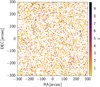 |
Fig. 11. Example of a simulated field of 10′ × 10′. Each point represents a simulated galaxy and is colour coded depending on its redshift. |
4. Validation and discussion
In this section we perform some analyses to validate the simulated catalogues obtained using SPRITZ. In all the figures we show as reference the simulation with kΦ = −1 (see Eq. (2)), but we include the results considering the other high-z extrapolations in the uncertainties.
It is worth mentioning that the conversion between the LIR and any other quantity is fixed to a specific value that depends on the template associated with each simulated galaxy. As the number of considered templates is limited to 35 templates from Polletta et al. (2007), Rieke et al. (2009), and Bianchi et al. (2018), the ratio of LIR to other quantities, such as stellar mass and luminosities at specific wavelengths, is discrete. To limit such issue, we considered the observational scatter associated with any assumed empirical relation as well as the probability distribution of the different parameters derived by MAGPHYS or SED3FIT.
As investigated by Gruppioni & Pozzi (2019), the Herschel IR LF considered in this work is in perfect agreement with results from independent works at various wavelengths, including IR (Rodighiero et al. 2010; Lapi et al. 2011; Marchetti et al. 2016; Rowan-Robinson et al. 2016), radio (Novak et al. 2017), and CO observations (Vallini et al. 2016; Riechers et al. 2019). In addition, the extrapolations done at z > 3, in particular the extrapolation with kΦ = −1, are consistent with the constraints obtained from the continuum LF up to z ∼ 6 of ALMA serendipitous detections in the ALPINE survey (Gruppioni et al. 2020), as shown in Fig. 12.
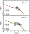 |
Fig. 12. Observed IR LFs derived in the ALPINE survey (black circles, Gruppioni et al. 2020) at z = 3.5 − 4.5 (top) and z = 4.5 − 6 (bottom). The empty circles are below the completeness limits. The ALMA IR LFs are compared with the four extrapolations of the total Herschel LFs used in this work to extract simulated galaxies at z > 3 (coloured solid lines). |
In this section, we compare the derived number counts in different bands, the stellar mass function, the SFR-stellar mass relation, the X-ray, FUV and K-band LFs, and an AGN diagnostic diagram (i.e., BPT diagram; Baldwin et al. 1981) with various observational results from previous works.
4.1. Number counts
We start our tests by comparing the differential number counts of the SPRITZ simulation with those of the Cosmic Assembly Near-infrared Deep Extragalactic Legacy Survey (CANDELS; Grogin et al. 2011) in the GOODS-S field (Guo et al. 2013). Broad-band filters cover from the U band up to the 8 μm Spitzer-IRAC band. The comparison is shown in Fig. 13, where we also include data from the Galaxy And Mass Assembly survey (GAMA; Hill et al. 2011) and the AKARI telescope (Murata et al. 2014). We corrected these observations for the difference in the filters by computing the median ratio of the fluxes derived considering the CANDELS filters and the closest GAMA or AKARI filters, which are both included in the SPRITZ simulation. To avoid spurious sources we only reported CANDELS observations above the 5σ detection limit reported by Guo et al. (2013). Neither the GAMA, AKARI, nor the CANDELS data are corrected for completeness, but we report only AKARI data above 90% completeness, as derived in their paper. Completeness levels are difficult to estimate for the CANDELS GOODS-S survey, given its non-homogeneous observational depth (see Guo et al. 2013). In any case, we obtained an approximate estimation of the 50% completeness level by deriving the magnitude at which the number counts deviate by more than a factor of 2 from a power law. A similar method was tested by Guo et al. (2013) on the Ks band. We report the estimated 50% completeness in Fig. 13, but the estimates at 5.6 and 8 μm may be underestimated as the number counts at these wavelengths deviate significantly from a power law.
 |
Fig. 13. Differential number counts of the SPRITZ simulated galaxies from the U band to the near-IR with high-redshift extrapolation kΦ = −1 (Eq. (2), solid black line). The shaded regions show the uncertainties due to the high-z extrapolation and the 1σ errors of the LFs and GSMF used to generate simulated galaxies. Observations in the same bands of the CANDELS GOODS-S survey (filled circles, Guo et al. 20130 and data from the GAMA survey (filled squares, Hill et al. 2011) and the AKARI telescope (filled diamonds, Murata et al. 2014), both corrected for the differences in the broad-band filters, are also shown. For clarity, only one every four data points of the GAMA survey are shown. The dotted vertical black lines show a rough estimate of the 50% completeness level for CANDELS data. |
The SPRITZ differential number counts agree with observations over a large range in magnitudes. The CANDELS observations show some bias at bright magnitudes owing to the small area covered by the survey in GOODS-S, as visible when the GAMA or AKARI data in similar filters are available. Some inconsistencies are present for the HST/F098M filter, but they are not present in adjacent bands. This suggests that there may be some specific and relative narrow features that only affecting data in that band. The considered filter is only included in the CANDELS survey and not in the GAMA or AKARI surveys; therefore we cannot check the presence of some observational biases. In some filters, number counts are slightly overestimated in the SPRITZ simulation at intermediate magnitudes and, given the just mentioned completeness level, this cannot be explained fully with observational incompleteness. Except for the HST/F098M filter, all estimates are overall within the model uncertainties.
We compare the differential number counts, normalised to the Euclidean slope, of SPRITZ galaxies in the mid- and far-IR together with results from the literature (Fig. 14). In particular, we consider differential normalised number counts derived using Spitzer (Papovich et al. 2004; Le Floc’h et al. 2009), Herschel (Berta et al. 2011; Magnelli et al. 2013; Clements et al. 2010; Béthermin et al. 2012; Valiante et al. 2016), AKARI (Pearson et al. 2012; Murata et al. 2014; Davidge et al. 2017), SCUBA-2 (Geach et al. 2013, 2017; Hsu et al. 2016; Wang et al. 2017; Zavala et al. 2017), and ALMA observations (Stach et al. 2018; Béthermin et al. 2020). The SPRITZ differential normalised number counts agree overall with observations over a large range of wavelengths and fluxes. There are however some discrepancies, in particular at 18 μm, where number counts are overestimated, and at 24 μm where the peak in the normalised number counts is slightly underestimated. At 100 μm some discrepancies are present with observations from the AKARI All-Sky Survey (Pearson et al. 2012) for sources brighter than 104 mJy, which mainly correspond to low-z spirals. However, these are also galaxies from which beam corrections are expected to be large in the AKARI observations because they are generally extended Clements et al. (2019). This effect would underestimate some AKARI fluxes and would move the tension to larger fluxes; or, in case only some galaxies are affected by this issue, would flatten the observed normalised number counts, thereby reducing the tension with the simulation. At longer wavelengths, λ > 500 μm, some discrepancies are present in the bright-end regime (i.e., fν > 102 mJy), mainly owing to the AGN1 and AGN2 populations at z = 1–4. This may indicate the necessity to include an AGN template with a less prominent cold-dust component.
 |
Fig. 14. Differential number counts normalised to the Euclidean slope of the SPRITZ simulated galaxies in the mid- and far-IR with high-redshift extrapolation kΦ = −1 (Eq. (2), solid black line). The shaded regions show the uncertainties due to the high-z extrapolation and 1σ errors of the LFs and GSMF used to generate simulated galaxies. Several observed values present in the literature are also shown (Papovich et al. 2004; Le Floc’h et al. 2009; Clements et al. 2010; Berta et al. 2011; Béthermin et al. 2012, 2020; Pearson et al. 2012; Geach et al. 2013; Magnelli et al. 2013; Murata et al. 2014; Hsu et al. 2016; Valiante et al. 2016; Davidge et al. 2017; Geach et al. 2017; Wang et al. 2017; Zavala et al. 2017; Stach et al. 2018). The thin coloured lines represent the normalised number counts for the different galaxy populations considered in SPRITZ: spirals (light green line), SBs (cyan line), SF-AGN (dark-green line), SB-AGN (orange line), AGN type-1 (blue line), AGN type-2 (magenta line), elliptical galaxies (red line), and irregular galaxies (brown line). |
4.2. Stellar mass function
In Fig. 15 we report the comparison between the stellar mass function of SPRITZ galaxies and the data available in the literature (Ilbert et al. 2013; Caputi et al. 2015; Grazian et al. 2015; Davidzon et al. 2017). Galaxies are selected in the Ks band in Ilbert et al. (2013), at 4.5 μm in Caputi et al. (2015), in the HST/F160W at 1.6 μm in Grazian et al. (2015), and in the stacked zYJHK image in Davidzon et al. (2017). These results are corrected for completeness, as mentioned in each corresponding paper. The results from the SPRITZ simulations are shown for the master catalogue before applying any observational selection to mimic any spectro-photometric survey. We converted the observed stellar mass function to the same IMF (Chabrier 2003) and cosmology used in this work, when necessary.
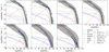 |
Fig. 15. Stellar mass function of the SPRITZ simulation at different redshifts (thick solid black line), with high-redshift extrapolation kΦ = −1 (Eq. (2)) and −4 (thick dotted black line). The grey shaded area shows the uncertainties arising from the high-z extrapolation, the different torus library considered, the 1σ value derived from the probability distribution of the stellar mass of each SED template, and the 1σ errors of the LFs and GSMF used to derive simulated galaxies. Some of the values present in the literature are reported: Ilbert et al. (2013, green crosses), Davidzon et al. (2017, blue circles), Caputi et al. (2015, cyan squares) and Grazian et al. (2015, magenta triangles). The thin coloured lines represent the stellar mass functions for the different galaxy populations considered in SPRITZ: spirals (light green line), SBs (cyan line), SF-AGN (dark green line), SB-AGN (orange line), AGN type-1 (blue line), AGN type-2 (magenta line), elliptical galaxies (red line), and irregular galaxies (brown line). |
The SPRITZ stellar-mass function is overall consistent with the observed values in the high-mass regime and low-mass end. The high-mass end is dominated by elliptical galaxies up to z = 2 and by SB, SB-AGN, and SF-AGN at higher redshifts. This change in the bright end, from dominated by elliptical to dominated by SB-AGN, suggests that SB-AGN may be indicated as the progenitors of elliptical galaxies. The low-mass end is instead, not surprisingly, dominated by dwarf irregular galaxies. At z > 3 the simulation with kΦ = −1 (Eq. (2)) brings to an overestimation of the faint end of the stellar mass function, while the simulation with kΦ = −4 agrees better with the observations. Therefore, while the IR LF favours the kΦ = −1 high-z extrapolation for Herschel galaxies (see Fig. 12), the stellar mass function favours a steeper evolution (i.e., kΦ = −4 (Eq. (2))) for irregular galaxies. It is however necessary to take into account that large uncertainties on the predictions are present at low masses at z < 3 end at all masses at higher redshifts. These mainly result from the extrapolations performed in the simulation because the Herschel data probed z < 3 and relatively bright galaxies. Future IR observations reaching much fainter fluxes may help anchor the high-z and low-mass extrapolations and reduce the scatter on the predictions.
4.3. SFR and stellar-mass plane
The majority of star-forming galaxies show a tight relation between their current SFR and their stellar mass, historically called the main sequence of star-forming galaxies (Brinchmann et al. 2004; Noeske et al. 2007). This relation has been interpreted as the result of the interplay of secular and stochastic effects that boost or suppress the SFR (Peng et al. 2014; Tacchella et al. 2016). Galaxies with suppressed star formation are below this almost-linear relation, while SB galaxies, featuring a temporary boost on their SFR, lie above the main sequence. The number of SB galaxies is very low in the local Universe (Rodighiero et al. 2011; Sargent et al. 2012) with a possible strong increase in their fraction with redshift (Caputi et al. 2017; Bisigello et al. 2018)
In Fig. 16 we show the distribution of galaxies simulated with SPRITZ in the SFR–stellar mass plane. No scatter has been considered for the SFR and stellar mass associated with each simulated galaxy. The results are shown for the master catalogue before any flux selection. For comparison, we report the sequence of normal star-forming galaxies derived by Elbaz et al. (2011), Speagle et al. (2014), Caputi et al. (2017), Santini et al. (2017), and Bisigello et al. (2018) and that occupied by SB derived by Caputi et al. (2017) and Bisigello et al. (2018). The Elbaz et al. (2011) sample comprises galaxies detected in the far-IR and their SFR is derived directly from the total IR luminosity. Speagle et al. (2014) derived the sequence using a large set of results available in the literature, from UV and IR data, carefully taking into account possible biases. In Bisigello et al. (2018), the sequence is derived considering a sample of optically selected galaxies with multiwavelength observations and the SFRs are derived from the dust-corrected UV fluxes complemented, when possible, by IR observations. The work by Caputi et al. (2017) considers instead galaxies detected at rest-frame optical wavelengths with multiwavelength observations and SFRs are derived from the dust-corrected Hα fluxes, as obtained from the observed flux excess in the available broad-band filters. Finally, Santini et al. (2017) consider a sample of optically selected galaxies, including also gravitational lenses to push the analysis to low-mass and high-z systems, and SFRs are derived from the dust-corrected UV fluxes. We chose to compare with works that apply different techniques and span different redshifts and stellar masses to avoid large biases in the comparison with our simulation. The SFR in SPRITZ includes both the ‘unobscured’ component, as derived from the IR, and the obscured component from the UV; these are computed after removing the AGN contribution.
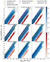 |
Fig. 16. Stellar mass vs. SFR at different redshifts for simulated SPRITZ galaxies with high-redshift extrapolation kΦ = −1 (Eq. (2)). Blue shows the distribution of galaxies derived from the IR LF or the irregular GSFM, while red indicates the distribution of elliptical galaxies derived from the K-band LF. The colour gradients show the number of galaxy in 1 deg2 and these are in logarithmic scale, as shown on the right for star-forming galaxies (top colour bar) and ellipticals (bottom colour bar). The different lines show the observed position of normal star-forming galaxies as derived by Elbaz et al. (2011, dash-dot-dot-dotted green line), Speagle et al. (2014, dotted black line), Caputi et al. (2017, dash-dot-dotted yellow line), Santini et al. (2017, dash-dotted light green line), Bisigello et al. (2018, dashed orange line), and the relation derived for SBs by Caputi et al. (2017, pink dash-dot-dotted lines) and Bisigello et al. (2018, magenta dashed lines). |
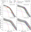 |
Fig. 17. Luminosity function at 8 μm for all galaxies simulated with SPRITZ (solid black tick line), with high-redshift extrapolation kΦ = −1 (Eq. (2)). The grey area shows the uncertainties due to the high-z extrapolation and 1σ errors of the GSFM, IR, and K-band LFs used to generate simulated galaxies. The LF for the different sub-populations is also shown: spirals (green line), SBs (cyan line), the two composite populations SF-AGN (dark green line) and SB-AGN (orange line), AGN type-1 (blue line), AGN type-2 (magenta line), elliptical galaxies (red line), and irregular galaxies (brown line). The observed 8 μm LFs by Rodighiero et al. (2010, red squares), Caputi et al. (2007, blue circles), Goto et al. (2015, 2019, green triangles), and Magnelli et al. (2011, light blue stars) are also represented. |
Elliptical galaxies have stellar masses and SFRs consistent with the quiescent population, and the elliptical galaxies occupy the area ∼2 dex below the sequence of normal star-forming galaxies. All the other simulated galaxies occupy the area expected for star-forming and SB galaxies at the different redshifts. Simulated galaxies form a sequence that at low-z is steeper than that observed by Speagle et al. (2014). However, Bisigello et al. (2018) shows that the slope estimated considering only relative massive galaxies (i.e., log10(M∗/M⊙) > 9.5) and a classical χ2 fitting method, as done by Speagle et al. (2014), can produce a flattening of the derived main sequence. For comparison, at the same redshift, Elbaz et al. (2011) derive a steeper main sequence and a smaller normalisation than Speagle et al. (2014). This relation shows a SFR ∼0.05 (0.5) dex that is below the average SFR of the star-forming galaxies in our sample at log(M/M⊙) ∼ 11 (8). At z ∼ 4.5, there are few galaxies with SFR as high as observed by Caputi et al. (2017), showing that more extreme SB templates may be necessary to reproduce these observations. Indeed, SB galaxies in the SPRITZ simulation are above the MS at z < 2, but they have sSFR consistent with the MS at z > 2. At even higher redshifts, i.e., z = 5 − 7, simulated star-forming galaxies agree with predictions from Speagle et al. (2014) at stellar masses above 1010 M⊙, while they are generally below the expected main sequence at lower stellar masses. Discrepancies are larger when considering observations by Santini et al. (2017), whose data point out a larger normalisation for the main sequence at such high-z. It is however necessary to take into account that the work by Speagle et al. (2014) is limited to the brightest galaxies, while the work by Santini et al. (2017) is limited in statistics at this very high-z. Future observations over large areas of galaxies at z > 5 will help to anchor the main sequence and the SB locus.
The linear relation among SFR and stellar mass observed in our simulation is not surprising because the ratio of stellar mass to IR/UV luminosity is constant for each template and all the templates considered, excluding the elliptical templates, have SFR and stellar masses that are consistent with normal star-forming systems or SBs. However, the evolution with redshift and the exact slope of the relation is dictated by the evolution of the considered IR LF and the fraction of the templates used for describing each galaxy population at different redshift and LIR. Therefore, since the evolution of the LF is consistent with the observed evolution of the SFR–stellar mass relation, the evolution of the main sequence of star formation is simply dictated by the luminosity (∼SFR) evolution.
4.4. Luminosity functions
In the next sections we compare the SPRITZ LF with observations available in the literature, focussing on some representative wavelengths spanning from the X-ray to the radio.
4.4.1. 8 μm
We now discuss the comparison from the 8 μm LF. In particular, we compare the SPRITZ simulation with results from Caputi et al. (2007), Rodighiero et al. (2010), and Magnelli et al. (2011), which are all obtained from a sample of galaxies observed with Spitzer at 24 μm. We complement this comparison with the results by Goto et al. (2015, 2019) using AKARI observations. We do not show higher redshifts as there are no available observations. The observations and the SPRITZ simulation show a large scatter, but they generally agree with each other at any redshift and luminosity. A light overestimation may be present in the SPRITZ simulation in the faint end at z ∼ 0.5, but few observations are available in this luminosity range (i.e., L8 μm < 1010 L⊙).
4.4.2. K band
Another test we perform to validate our results consists in reproducing the observed K-band LF with our simulated catalogue. We show the K-band LF of SPRITZ galaxies in Fig. 18 together with the observed LF by Mortlock et al. (2017), Cirasuolo et al. (2007), and Beare et al. (2019). The LF is generally reproduced well. The knee of the K-band LF of SPRITZ galaxies is consistent with observations up to z ∼ 3.5, while small deviations from observations are present in the bright and faint-end regime and at z > 3.5. Below z < 1.25 the bright-end regime is dominated by elliptical galaxies with spirals and irregulars dominating at faint magnitudes (MKs > −20). Spiral galaxies and AGN-1 are also present at extremely bright magnitudes (i.e., MKs < −25), where the number densities are generally below those probed by observations. At higher redshift, composite systems and AGN dominate the bright end; there is a decreasing contribution of elliptical galaxies. Some differences in the bright end at z > 1.25 may arise from the selection done in the literature, as bright X-ray sources are removed before deriving the observed K-band LF.
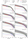 |
Fig. 18. Same as Fig. 17, but for the K-band LF. The observed K-band LFs are represented by Mortlock et al. (2017, red squares), Cirasuolo et al. (2007, blue circles), and Beare et al. (2019, green triangles) in the overlapping redshift bins. |
The agreement between the simulated and the observed K-band LF is in line with the consistency between the SPRITZ and the observed stellar mass function analysed in Sect. 4.2, considering that the K band is dominated by the light of the old stellar populations and is therefore a relative good tracer of the stellar mass. We can conclude that the K-band LF of SPRITZ simulated galaxies slightly overestimates the observed K-band LF at z > 3.5, where few observations are available, while the simulated LF generally agrees with observations at other redshifts. The Spritz LF is dominated by AGN in the bright-end regime at high-z and the absence of AGN in the literature derivations could be responsible for this inconsistency.
4.4.3. B band
In this section we compare the rest-frame B-band LF of the SPRITZ simulation with observations available in the literature. In particular, we considered the B-band LF by Beare et al. (2015), Fritz et al. (2014), and Gabasch et al. (2004), whose samples are selected in the observed i band;, the work by Dahlen et al. (2005) using R- and K-band selected galaxies; results by Poli et al. (2003) using i- and K-band selected galaxies; and the LF by Marchesini et al. (2007) derived from a sample of K-selected galaxies. The comparison is shown in Fig. 19.
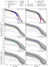 |
Fig. 19. Same as Fig. 17, but for the B-band LF. The observed B-band LFs are represented by Fritz et al. (2014, red squares), Beare et al. (2015, blue circles), Dahlen et al. (2005, green triangles), Poli et al. (2003, magenta upside-down triangles), Gabasch et al. (2004, pink pentagon), and Marchesini et al. (2007, light blue stars) in the overlapping redshift bins. |
At z < 1.25, the bright end of the B-band LF is generally overestimated in the SPRITZ simulation similarly to the K-band LF. On the other hand, the faint end of the B-band LF is remarkably similar to observations, at least at z > 0.75. This reassures on the validity of the approach considered to introduce irregular galaxies, which dominate the faint end. At z > 1.25 the SPRITZB-band LF generally agrees with the observations, at least in the magnitude range covered by the observations. However, few studies are present in the literature showing a large scatter (see z ∼ 3). In the plot we also report the SPRITZ B-band LF without considering AGN because they are at least partially removed in some of the considered studies (i.e., in Fritz et al. 2014 and Beare et al. 2015). However, the two LF do not differ significantly because AGN never dominate the B-band LF except in the very bright end, which has not been covered by the considered observations.
4.4.4. Far-ultraviolet
We perform the next comparison of SPRITZ simulation with the observed LFs by analysing the FUV regime. Figure 20 shows the LF derived at 1600 Å for SPRITZ simulated galaxies and the observed LF for galaxies and QSO by McGreer et al. (2013), Akiyama et al. (2018), and Schindler et al. (2019) at 1450 Å; by Moutard et al. (2020) at 1546 Å; by Oesch et al. (2010), Parsa et al. (2016), and Adams et al. (2020) at 1500 Å; by Bouwens et al. (2015) at 1600 Å; and by Reddy & Steidel (2009) at 1700 Å. Observations by Ono et al. (2018) correspond to rest frame between 1230 and 1600 Å, depending on redshift. The data by Croom et al. (2009) and Ross et al. (2013) are converted to 1450 Å.
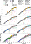 |
Fig. 20. Same as Fig. 17, but for the LF at 1600 Å. Our simulation is compared with other data from the literature (see legend). |
The bright end of the UV LF is dominated by unobscured QSO, which are equivalent to the AGN1 population considered in the simulation. We take advantage of the separation of the LF of this galaxy population to improve the IR LF of AGN1 and AGN2 in the SPRITZ simulation (see Sect. 2.1.2 and Appendix A), therefore by construction the bright-end UV LF of the SPRITZ simulation agrees with observations up to high-z. The part dominated by galaxies agrees with observations at all redshifts, except for galaxies at z < 0.75 in the bright-end regime (i.e., MUV < −20. At z > 2); the galaxy LF is consistent with observations, but tends to slightly underestimate the faint end. This light discrepancy in the faint-end slope may be explained with a dust-poor population of galaxies missed by the Herschel observations and not completely described by the irregular population. It has been shown by observations that the fraction of dusty objects and the amount of dust extinction decreases towards faint FUV magnitudes (Bouwens et al. 2016). However these two quantities seem to have little or no evolution at high-z, which is in line with our underestimation of the faint-end slope that remains similar between z = 2 and 5. On the other hand, it is also possible that the SED templates considered for irregular galaxies, which dominate the galaxy population with M1600 Å > −21, are not representative for all redshifts. Indeed, for all the galaxy population derived from the Herschel LF, we considered different probabilities for each template based on observations and depending on redshift and LIR. On the other hand, we considered a constant probability for the three SED templates of irregular galaxies. More observations are necessary to verify the validity of this assumption. However, despite the large distance in wavelength between the basis of the SPRITZ simulations (e.g., mid- or far-IR) and the UV regime, the overall agreement between data and model is very good.
4.4.5. X-ray
In Fig. 21 we compare the hard X-ray LF obtained with the SPRITZ simulation with various X-ray observations (Aird et al. 2010, 2015; Miyaji et al. 2015; Vito et al. 2018; Wolf et al. 2021). At low-z the SPRITZ LF is consistent with observations, but at increasing redshift the faint end starts to be overestimated. This discrepancy is reduced if we exclude from the comparison heavily obscured AGN (i.e., log10(NH/cm−2) > 23) that can be missed by X-ray observations or whose intrinsic X-ray luminosity may be underestimated. The bright end of the LF is consistent with observations within 1σ even if it is generally overestimated. This happens even at z ∼ 6, taking into account that the X-ray LF by Wolf et al. (2021) is a conservative estimation, but it is in any case derived from a single object.
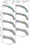 |
Fig. 21. Luminosity function at 2–10 keV for all AGN simulated with SPRITZ (solid black line) with high-redshift extrapolation kΦ = −1 (Eq. (2)) and for the sub-sample of AGN with log10(NH/cm−2) < 23 (dotted black line). The grey area shows the uncertainties due to the conversion from the L12 μm to L2 − 10 keV, the use of different torus models, and the 1σ errors of the IR LFs used to derive the simulated galaxies hosting an AGN. The LF for each different sub-population is also shown (see Fig. 17). The observed X-ray LFs by Wolf et al. (2021, purple star), Miyaji et al. (2015, cyan squares), Aird et al. (2010, red circles), Aird et al. (2015, green and orange triangles), and Vito et al. (2018, yellow diamonds) are reported. |
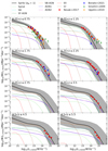 |
Fig. 22. Rest-frame LF at 1.4 GHz for all galaxies simulated with SPRITZ (solid black tick line) with high-redshift extrapolation kΦ = −1 (Eq. (2)), taking into account only the luminosity originated from the star formation activity. The grey areas indicate the uncertainties due to the high-z extrapolation, the different torus models included, and the 1σ errors of the GSMF, IR, and K-band LFs used to generate simulated galaxies. The LF for each different sub-population is also shown (see Fig. 17). The observed 1.4 GHz LFs, limited to the star-formation activity, by Novak et al. (2017, red squares), Bonato et al. (2021, blue circles), Smolčić et al. (2009, green trangles), and Upjohn et al. (2019, orange stars) are represented. |
It is necessary to take into account that the conversion to X-ray luminosity has more uncertainties that the UV or K-band luminosity analysed before. In the SPRITZ simulation the latter two mainly depend on the shape and evolution of the IR LF and on the templates associated with galaxies in different luminosity regimes. The X-ray luminosity in addition depends on the AGN-host galaxy decomposition and, finally, on the conversion from the luminosity at 12 μm to the X-ray luminosity. Moreover, we considered a single X-ray spectrum for all simulated AGN, as described in Sect. 2.2.2. All these effects contribute to generate the large uncertainties on the predictions as well as the discrepancy between the simulated and observed X-ray LF. From the point of view of observations, heavily obscured AGN can explain a possible underestimation of the observed faint-end slope. If we remove these sources from the SPRITZ simulation, the faint end of the new X-ray LF agrees with observations at redshift between 2 and 3.5, while at other redshifts the tension with observations is reduced. An additional possible source of error can be the mis-classification of low-luminosity AGN as galaxies in X-ray surveys as a result of their faint X-ray luminosity. Overall, the SPRITZ simulation can reproduce the shape and normalisation of the X-ray LF even if there are large uncertainties.
4.4.6. 1.4 GHz
In this section we compare the rest-frame 1.4 GHz LF in the SPRITZ simulation with results from the literature. In particular, we consider the LF at 1.4 GHz derived by Smolčić et al. (2009), Novak et al. (2017), Upjohn et al. (2019), and Bonato et al. (2021), considering only star formation activity (i.e., excluding radio-loud AGN). The 1.4 GHz luminosity is derived in SPRITZ from the IR LF using Eq. (7) and considering the component due to star formation of the IR luminosity. The SPRITZ simulation is overall in good agreement with observations at all redshifts and luminosities.
In Fig. 23 we show the comparison between the rest-frame 1.4 GHz LF of radio-loud AGN in SPRITZ and the same LF derived by Smolčić et al. (2017), Ceraj et al. (2018), Butler et al. (2019) and Bonato et al. (2021). The agreement between SPRITZ and observations is remarkable, considering the different selection criteria for radio-loud AGN applied in the literature and the uncertainties present in the simulation to select radio-loud AGN. Consistent with observations (e.g., Matthews et al. 1964), radio-loud AGN in SPRITZ are preferably hosted by elliptical galaxies, at least up to z = 1.75. This happens because elliptical galaxies dominate the low-z stellar-mass function and the fraction of radio-loud AGN depends on stellar mass (see Eq. (8)).
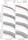 |
Fig. 23. Same as Fig. 22, but for radio-loud AGN. The observed 1.4 GHz LFs of radio-loud AGN by Ceraj et al. (2018, red squares), Bonato et al. (2021, blue circles), Smolčić et al. (2017, green trangles), and Butler et al. (2019, orange diamonds) are shown. |
4.5. AGN line diagnostics
The ratio of some nebular emission lines can give an indication concerning the nature of the source powering them, allowing us to discern between star-forming systems and AGN. The most used diagnostic, which allows us to separate AGN from H II regions, is the BPT diagram (Baldwin et al. 1981) which includes the ratio of the optical lines [O III] 5007 Å/Hβ and [N II] 6584 Å/Hα. We made use of such diagram to verify some nebular emission line flux implemented in the simulation. In Fig. 24, we show the position of the SPRITZ simulated galaxies in the BPT diagram, as derived from the master catalogue. We incorporated the nebular fluxes into the master catalogue before applying any observational scatter. The nebular line fluxes of the AGN component of the master catalogue were obtained by averaging the predictions of the models spanning the range of parameters described in Sect. 2.3. This flux is then normalised to the AGN accretion disk luminosity of each mock galaxy. When specific simulated galaxies are derived, considering the full probability distribution of physical parameters of the AGN models and the photometric errors, the [N II] 6584 Å/Hα ratios of AGN are not limited below log10([N II] 6584 Å/Hα) < − 0.37. The sharp limit at high [N II] 6584 Å/Hα values for galaxies without AGN is instead dictated by the asymptotic metallicity value of the considered mass metallicity relation (see Eq. (4)).
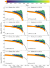 |
Fig. 24. BPT diagram for simulated galaxies. Data points are colour coded depending on the fraction of AGN measured in the IR. The solid black line shows the separation between AGN and H II region, as derived by Kewley et al. (2013b) at z ≤ 2.5. The dashed black line indicates the extrapolation of the same separation criteria at high reshifts. |
In the same figure we also report the semi-empirical line, evolving with redshift, that separates AGN from star-forming systems (Kewley et al. 2013b). The AGN-dominated systems lay above the separation line at all redshifts, while some of the galaxies with a fraction of AGN below 50%, as derived in the IR, are below the separation line at high-z. First, it is necessary to consider that these objects are the most uncertain because the AGN marginally contribute to the nebular emission lines considered in this work. Second, the separation line by Kewley et al. (2013b) is derived from data collected up to z ∼ 2.5, therefore its extrapolation at higher-z needs to be further verified.
5. Application: Predictions for JWST and OST
In this section we provide some examples of the application of SPRITZ to the construction of simulated catalogues, which is useful mostly for future space programmes. In particular, we simulated the following observations:
– JWST NIRCam observations in nine filters (F090W, F115W, F150W, F200W, F277W, F335M, F356W, F410M, and F444W) with 5σ depths between 29.5 and 30.6 AB magnitude and covering an area of 46 square arcmin. This follows the planned JADES-Deep survey (JWST Advanced Deep Extragalactic Survey), as prepared by the NIRSpec and NIRCam Guaranteed Time Observers (Rieke et al. 2019).
– A far-IR survey with OST over 500 deg2 area5 and with 5σ depths equal to 40 μJy and 1 mJy at 50 and 250 μm.
5.1. JWST
Figure 25 shows the number-redshift distribution and the stellar mass distributions at different redshifts for the JWST JADES-Deep simulated catalogue, considering only galaxies with mAB, F150W < 30.6. Irregular galaxies are expected to dominate the number counts of the survey, which is not surprising given that the flux cut corresponds in general to stellar masses as low as M* ∼ 108 M⊙ even at the highest redshift. However, these galaxies are expected to be detected in seven out of the nine considered filters, on average, with a median S/N ∼ 12. Excluding irregulars, at z > 4 we expect around 260 galaxies, all with an AGN contribution, but this number decreases to 29 when considering the most extreme redshift extrapolation (i.e., kΦ = −4). It is however necessary to point out that the redshift extrapolation with kΦ = −4 slightly underestimates the ALPINE IR LF at z ∼ 5 (see Fig. 12), so it is to be regarded as conservative prediction. The simulated catalogue also contains almost no AGN-dominated objects (AGN1 and AGN2) owing to a combination of depth and area. This shows the necessity of larger areas or pointed observations to study the AGN population with JWST. The number of irregular galaxies at z > 4 varies from 4 × 10² to 1.7 × 10³, showing the large uncertainties linked to this galaxy population.
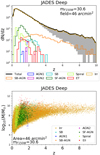 |
Fig. 25. Redshift distribution (top) and stellar mass vs. redshift (bottom) of the simulated galaxies obtained with the SPRITZ simulation for the JWST JADES-Deep survey, considering only galaxies brighter than mAB, F150W = 30.6. The different colours indicate different galaxy populations, as listed in the legend. On the top, the grey shaded area indicates uncertainties due to the high-z extrapolation of the different LFs. |
To further show the wealth of possible applications of the SPRITZ simulation, we generated simulated NIRCam images in different filters. In particular, we considered a single realisation of NIRCam point spread function, as simulated by WebbPSF (Perrin et al. 2012, 2014) considering the requirements optical path difference map6. Each simulated galaxy is considered as unresolved, but future developments may include morphological information. To generate the simulated images, we considered a gap of 43″ (47″) between the two NIRCam modules in the blue (red) filters, that is bands at wavelengths shorter (longer) than 2.3 μm (2.4 μm) and gaps of 4″ or 5″ between the 4 quadrants of each module, depending on the filter wavelengths. It is however necessary to consider that these distances are approximated because they may change after the launch6. The simulated image is shown in Fig. 26 combining three different filters, each shown with different colours: that is F090W (blue), F277W (green), and F44W (red). Simulated images in other filters are publicly available2.
 |
Fig. 26. Example of a NIRCam pointing in three filters: F090W (blue), F277W (green), and F44W (red). |
5.2. OST
In Fig. 27 we show our predictions for the redshift distribution and the LIR at different redshift of galaxies detected with OST. This mission is planned to have a collecting area of 5.9 m primary mirror at the moment of writing, and photometric filters observing at 50 and 250 μm. In addition, the great mapping capability will allow the observation of a sky area to be larger than that of the JWST. For this reason, the planned OST Medium Survey is expected to cover 500 deg2 with a 5σ depth of 40 μJy and 1 mJy at 50 and 250 μm. Both photometric filters are, at the moment, described as simple boxes and this is the reason behind some sharp features in the figure. At both 50 and 250 μm we predict that some irregular galaxies should be observable up to z ∼ 2, while elliptical galaxies will be limited to very low redshifts. On the other hand, spirals galaxies are expected to be observed at all redshifts at 50 μm and up to z = 5 at 250 μm. The SB-AGN population dominates the redshift distributions at both wavelengths at z > 2, while the remaining populations (i.e., SB, AGN1, AGN2, and SF-AGN) should be observable up to z = 10 at both wavelengths. Looking at the IR luminosity of the observed populations, we expect to detect ULIRG (i.e., LIR > 1012 L⊙) at all redshifts at 50 μm and at least up to z = 5 in the other filter. Observations at more moderate IR luminosities (i.e., LIR = 1011 L⊙) will instead be limited to z < 4 (z < 2) at 50 (250) μm.
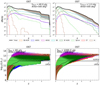 |
Fig. 27. Redshift distribution (top) and LIR vs. redshift (bottom) of the OST simulated catalogues covering 500 deg2. Galaxies detected in both photometric filters, that is the band centred at 50 μm (left) and that centred at 250 μm (right), are represented. The different colours indicate different galaxy populations, as listed in the legend. On the top, the grey shaded area indicates uncertainties due to the high-z extrapolation of the different LFs. |
These simulated catalogues were chosen to give an example of the possible application of the SPRITZ simulation and they are all publicly available2. Additional simulated catalogues involving these or other missions may be included in future releases or may be produced on demand.
6. Summary and conclusions
In this paper we present the new SPRITZ simulation to construct simulated catalogues for current and future facilities such as JWST and OST. The need for this new simulation is motivated by the difficulty of current semi-analytical and hydro-dynamical simulations to reproduce the observed number density of the most luminous IR galaxies.
The SPRITZ simulation is semi-empirical and starts from the IR LF based on Herschel sources up to z ∼ 3 (Gruppioni et al. 2013), complemented by the K-band LF of elliptical galaxies (Arnouts et al. 2007; Cirasuolo et al. 2007; Beare et al. 2019) and the GSMF of irregular galaxies by Huertas-Company et al. (2016). Both irregular and elliptical galaxies were not observed in sufficient number by Herschel and therefore it was necessary to include these separately as a simple extrapolation of the Herschel IR LF would not be sufficient to include them. We updated the Herschel IR LF of unobscured and obscured AGN by performing a combined fit of IR and FUV observations. We considered a series of empirical relations to assign several physical parameters as well as optical and IR emission features to each simulated galaxy, and we performed a host-AGN decomposition to estimate the contribution of AGN. Among the considered physical parameters are redshift, stellar mass, IR luminosity, SFR, hydrogen column density, X-ray luminosity, and 1.4 GHz luminosity. We created a simulated light cone by assigning a sky position to each simulated galaxies following a two-point angular correlation function, whose normalisation varies with stellar mass. For all these simulated galaxies we also derived the expected fluxes in different filters, from current and future facilities, such as SDSS, JWST, Euclid, and OST, as well as some low-resolution spectra, such as JWST MIRI-LR, and OST/OSS.
In this work we have shown that the SPRITZ simulation reproduces well a large number of observables, among which the number counts of galaxies from the U band to the far-IR, the stellar mass function, SFR-stellar mass plane, the IR LF at z > 37, the K-band, FUV, X-ray LFs, and the BPT diagram. In the future, the inclusion of additional observations and an increase in the number of considered SED templates may help to improve the simulation, reducing the few discrepancies as well as the uncertainties in the predictions.
We presented the use of SPRITZ to generate simulated catalogues, considering a JWST survey mimicking the planned JADES Deep and an OST survey of 500 deg2. Future releases may include additional surveys, not only for the considered missions but also for additional facilities (e.g., Euclid, Athena).
To conclude, the SPRITZ simulation is suitable for predictions for a broad set of future facilities operating at but not limited to IR wavelengths. This is possible by simulating realistic spectro-photometric data spanning a wide range in wavelengths.
For some parameters the used codes extract only the best value.
Using the code available in https://github.com/trevisanj/airvacuumvald
Predictions for this area are derived using the master catalogue, while a complete simulated catalogue is only available for 5 deg2.
Below z = 3 the IR LF function is reproduced by construction.
Acknowledgments
LB acknowledge financial support by the Agenzia Spaziale Italiana (ASI) under the research contract 2018-31-HH.0. CG, AF and FC acknowledge the support from grant PRIN MIUR 2017 20173ML3WW.
References
- Aaronson, M., & Olszewski, E. W. 1984, Nature, 309, 414 [NASA ADS] [CrossRef] [Google Scholar]
- Adams, N. J., Bowler, R. A. A., Jarvis, M. J., et al. 2020, MNRAS, 494, 1771 [CrossRef] [Google Scholar]
- Aird, J., Nandra, K., Laird, E. S., et al. 2010, MNRAS, 401, 2531 [Google Scholar]
- Aird, J., Coil, A. L., Georgakakis, A., et al. 2015, MNRAS, 451, 1892 [NASA ADS] [CrossRef] [Google Scholar]
- Akiyama, M., He, W., Ikeda, H., et al. 2018, PASJ, 70, S34 [NASA ADS] [CrossRef] [Google Scholar]
- Alcalde Pampliega, B., Pérez-González, P. G., Barro, G., et al. 2019, ApJ, 876, 135 [CrossRef] [Google Scholar]
- Antonucci, R. 1993, ARA&A, 31, 473 [Google Scholar]
- Arnouts, S., Walcher, C. J., Le Fèvre, O., et al. 2007, A&A, 476, 137 [NASA ADS] [CrossRef] [EDP Sciences] [Google Scholar]
- Asmus, D., Gandhi, P., Hönig, S. F., Smette, A., & Duschl, W. J. 2015, MNRAS, 454, 766 [NASA ADS] [CrossRef] [Google Scholar]
- Baes, M., Trčka, A., Camps, P., et al. 2020, MNRAS, 494, 2912 [CrossRef] [Google Scholar]
- Baldwin, J. A., Phillips, M. M., & Terlevich, R. 1981, PASP, 93, 5 [NASA ADS] [CrossRef] [EDP Sciences] [Google Scholar]
- Beare, R., Brown, M. J. I., Pimbblet, K., Bian, F., & Lin, Y.-T. 2015, ApJ, 815, 94 [NASA ADS] [CrossRef] [Google Scholar]
- Beare, R., Brown, M. J. I., Pimbblet, K., & Taylor, E. N. 2019, ApJ, 873, 78 [CrossRef] [Google Scholar]
- Berta, S., Magnelli, B., Nordon, R., et al. 2011, A&A, 532, A49 [NASA ADS] [CrossRef] [EDP Sciences] [Google Scholar]
- Berta, S., Lutz, D., Santini, P., et al. 2013, A&A, 551, A100 [NASA ADS] [CrossRef] [EDP Sciences] [Google Scholar]
- Bertola, F., & Galletta, G. 1978, ApJ, 226, L115 [NASA ADS] [CrossRef] [Google Scholar]
- Best, P. N., Kauffmann, G., Heckman, T. M., et al. 2005, MNRAS, 362, 25 [NASA ADS] [CrossRef] [Google Scholar]
- Béthermin, M., Le Floc’h, E., Ilbert, O., et al. 2012, A&A, 542, A58 [NASA ADS] [CrossRef] [EDP Sciences] [Google Scholar]
- Béthermin, M., Daddi, E., Magdis, G., et al. 2015, A&A, 573, A113 [NASA ADS] [CrossRef] [EDP Sciences] [Google Scholar]
- Béthermin, M., Fudamoto, Y., Ginolfi, M., et al. 2020, A&A, 643, A2 [CrossRef] [EDP Sciences] [Google Scholar]
- Bezanson, R., van der Wel, A., Straatman, C., et al. 2018, ApJ, 868, L36 [CrossRef] [Google Scholar]
- Bianchi, S., De Vis, P., Viaene, S., et al. 2018, A&A, 620, A112 [NASA ADS] [CrossRef] [EDP Sciences] [Google Scholar]
- Bisigello, L., Caputi, K. I., Colina, L., et al. 2016, ApJS, 227, 19 [NASA ADS] [CrossRef] [EDP Sciences] [Google Scholar]
- Bisigello, L., Caputi, K. I., Colina, L., et al. 2017, ApJS, 231, 3 [CrossRef] [Google Scholar]
- Bisigello, L., Caputi, K. I., Grogin, N., & Koekemoer, A. 2018, A&A, 609, A82 [NASA ADS] [CrossRef] [EDP Sciences] [Google Scholar]
- Bonato, M., De Zotti, G., Leisawitz, D., et al. 2019, PASA, 36 [CrossRef] [Google Scholar]
- Bonato, M., Prandoni, I., De Zotti, G., et al. 2021, MNRAS, 500, 22 [Google Scholar]
- Bouwens, R. J., Illingworth, G. D., Oesch, P. A., et al. 2015, ApJ, 803, 34 [Google Scholar]
- Bouwens, R. J., Aravena, M., Decarli, R., et al. 2016, ApJ, 833, 72 [NASA ADS] [CrossRef] [Google Scholar]
- Bradford, C. M., Cameron, B., Moore, B., et al. 2018, in Space Telescopes and Instrumentation 2018: Optical, Infrared, and Millimeter Wave, eds. M. Lystrup, H. A. MacEwen, G. G. Fazio, N. Batalha, N. Siegler, & E. C. Tong, International Society for Optics and Photonics (SPIE), 10698, 385 [Google Scholar]
- Brandl, B. R., Bernard-Salas, J., Spoon, H. W. W., et al. 2006, ApJ, 653, 1129 [NASA ADS] [CrossRef] [Google Scholar]
- Brinchmann, J., Charlot, S., White, S. D. M., et al. 2004, MNRAS, 351, 1151 [NASA ADS] [CrossRef] [Google Scholar]
- Bruzual, G., & Charlot, S. 2003, MNRAS, 344, 1000 [NASA ADS] [CrossRef] [Google Scholar]
- Butler, A., Huynh, M., Kapińska, A., et al. 2019, A&A, 625, A111 [NASA ADS] [CrossRef] [EDP Sciences] [Google Scholar]
- Caputi, K. I., Lagache, G., Yan, L., et al. 2007, ApJ, 660, 97 [NASA ADS] [CrossRef] [Google Scholar]
- Caputi, K. I., Ilbert, O., Laigle, C., et al. 2015, ApJ, 810, 73 [NASA ADS] [CrossRef] [Google Scholar]
- Caputi, K. I., Deshmukh, S., Ashby, M. L. N., et al. 2017, ApJ, 849, 45 [NASA ADS] [CrossRef] [Google Scholar]
- Casali, M., Adamson, A., Alves de Oliveira, C., et al. 2007, A&A, 467, 777 [NASA ADS] [CrossRef] [EDP Sciences] [Google Scholar]
- Ceraj, L., Smolčić, V., Delvecchio, I., et al. 2018, A&A, 620, A192 [NASA ADS] [CrossRef] [EDP Sciences] [Google Scholar]
- Chabrier, G. 2003, PASP, 115, 763 [Google Scholar]
- Charlot, S., & Fall, S. M. 2000, ApJ, 539, 718 [Google Scholar]
- Cigan, P., Young, L., Cormier, D., et al. 2016, AJ, 151, 14 [NASA ADS] [CrossRef] [Google Scholar]
- Cirasuolo, M., McLure, R. J., Dunlop, J. S., et al. 2007, MNRAS, 380, 585 [NASA ADS] [CrossRef] [Google Scholar]
- Clements, D. L., Rigby, E., Maddox, S., et al. 2010, A&A, 518, L8 [NASA ADS] [CrossRef] [EDP Sciences] [Google Scholar]
- Clements, D. L., Rowan-Robinson, M., Pearson, C., et al. 2019, PASJ, 71, 7 [CrossRef] [Google Scholar]
- Croom, S. M., Richards, G. T., Shanks, T., et al. 2009, MNRAS, 399, 1755 [NASA ADS] [CrossRef] [Google Scholar]
- da Cunha, E., Charlot, S., & Elbaz, D. 2008, MNRAS, 388, 1595 [Google Scholar]
- da Cunha, E., Charmandaris, V., Díaz-Santos, T., et al. 2010, A&A, 523, A78 [NASA ADS] [CrossRef] [EDP Sciences] [Google Scholar]
- Dahlen, T., Mobasher, B., Somerville, R. S., et al. 2005, ApJ, 631, 126 [NASA ADS] [CrossRef] [Google Scholar]
- Davidge, H., Serjeant, S., Pearson, C., et al. 2017, MNRAS, 472, 4259 [CrossRef] [Google Scholar]
- Davidzon, I., Ilbert, O., Laigle, C., et al. 2017, A&A, 605, A70 [NASA ADS] [CrossRef] [EDP Sciences] [Google Scholar]
- Decarli, R., Walter, F., Gónzalez-López, J., et al. 2019, ApJ, 882, 138 [Google Scholar]
- Delhaize, J., Smolčić, V., Delvecchio, I., et al. 2017, A&A, 602, A4 [NASA ADS] [CrossRef] [EDP Sciences] [Google Scholar]
- Delvecchio, I., Smolčić, V., Zamorani, G., et al. 2018, MNRAS, 481, 4971 [NASA ADS] [CrossRef] [Google Scholar]
- Dopita, M. A., Kewley, L. J., Sutherland, R. S., & Nicholls, D. C. 2016, Ap&SS, 361, 61 [NASA ADS] [CrossRef] [Google Scholar]
- Dowell, C. D., Conley, A., Glenn, J., et al. 2014, ApJ, 780, 75 [NASA ADS] [CrossRef] [Google Scholar]
- Duras, F., Bongiorno, A., Ricci, F., et al. 2020, A&A, 636, A73 [CrossRef] [EDP Sciences] [Google Scholar]
- Elbaz, D., Dickinson, M., Hwang, H. S., et al. 2011, A&A, 533, A119 [NASA ADS] [CrossRef] [EDP Sciences] [Google Scholar]
- Fazio, G. G., Hora, J. L., Allen, L. E., et al. 2004, ApJS, 154, 10 [NASA ADS] [CrossRef] [Google Scholar]
- Feltre, A., Hatziminaoglou, E., Fritz, J., & Franceschini, A. 2012, MNRAS, 426, 120 [Google Scholar]
- Feltre, A., Charlot, S., & Gutkin, J. 2016, MNRAS, 456, 3354 [Google Scholar]
- Ferland, G. J., Porter, R. L., van Hoof, P. A. M., et al. 2013, Rev. Mex. Astron. Astrofis., 49, 137 [Google Scholar]
- Foreman-Mackey, D. 2016, J. Open Source Softw., 1, 24 [Google Scholar]
- Foreman-Mackey, D., Hogg, D. W., Lang, D., & Goodman, J. 2013, PASP, 125, 306 [Google Scholar]
- Fritz, J., Franceschini, A., & Hatziminaoglou, E. 2006, MNRAS, 366, 767 [Google Scholar]
- Fritz, A., Scodeggio, M., Ilbert, O., et al. 2014, A&A, 563, A92 [NASA ADS] [CrossRef] [EDP Sciences] [Google Scholar]
- Gabasch, A., Bender, R., Seitz, S., et al. 2004, A&A, 421, 41 [NASA ADS] [CrossRef] [EDP Sciences] [Google Scholar]
- García-González, J., Alonso-Herrero, A., Hernán-Caballero, A., et al. 2016, MNRAS, 458, 4512 [NASA ADS] [CrossRef] [Google Scholar]
- García-Burillo, S., Combes, F., Ramos Almeida, C., et al. 2019, A&A, 632, A61 [CrossRef] [EDP Sciences] [Google Scholar]
- Gardner, J. P., Mather, J. C., Clampin, M., et al. 2009, in Astrophysics in the Next Decade, eds. H. A. Thronson, M. Stiavelli, & A. Tielens (Dordrecht:: Springer), 1 [Google Scholar]
- Geach, J. E., Chapin, E. L., Coppin, K. E. K., et al. 2013, MNRAS, 432, 53 [NASA ADS] [CrossRef] [Google Scholar]
- Geach, J. E., Dunlop, J. S., Halpern, M., et al. 2017, MNRAS, 465, 1789 [Google Scholar]
- Gilli, R., Comastri, A., & Hasinger, G. 2007, A&A, 463, 79 [NASA ADS] [CrossRef] [EDP Sciences] [Google Scholar]
- Gilmozzi, R., & Spyromilio, J. 2008, in Ground-based and Airborne Telescopes II, eds. L. M. Stepp, & R. Gilmozzi, SPIE Conf. Ser., 7012, 701219 [CrossRef] [Google Scholar]
- Glasse, A., Rieke, G. H., Bauwens, E., et al. 2015, PASP, 127, 686 [NASA ADS] [CrossRef] [Google Scholar]
- Goto, T., Oi, N., Ohyama, Y., et al. 2015, MNRAS, 452, 1684 [CrossRef] [Google Scholar]
- Goto, T., Oi, N., Utsumi, Y., et al. 2019, PASJ, 71, 30 [CrossRef] [Google Scholar]
- Goudfrooij, P., & de Jong, T. 1995, A&A, 298, 784 [NASA ADS] [Google Scholar]
- Grazian, A., Fontana, A., Santini, P., et al. 2015, A&A, 575, A96 [NASA ADS] [CrossRef] [EDP Sciences] [Google Scholar]
- Griffin, M. J., Abergel, A., Abreu, A., et al. 2010, A&A, 518, L3 [EDP Sciences] [Google Scholar]
- Grogin, N. A., Kocevski, D. D., Faber, S. M., et al. 2011, ApJS, 197, 35 [NASA ADS] [CrossRef] [Google Scholar]
- Gruppioni, C., & Pozzi, F. 2019, MNRAS, 483, 1993 [NASA ADS] [CrossRef] [Google Scholar]
- Gruppioni, C., Pozzi, F., Andreani, P., et al. 2010, A&A, 518, L27 [NASA ADS] [CrossRef] [EDP Sciences] [Google Scholar]
- Gruppioni, C., Pozzi, F., Zamorani, G., & Vignali, C. 2011, MNRAS, 416, 70 [NASA ADS] [CrossRef] [Google Scholar]
- Gruppioni, C., Pozzi, F., Rodighiero, G., et al. 2013, MNRAS, 432, 23 [NASA ADS] [CrossRef] [Google Scholar]
- Gruppioni, C., Calura, F., Pozzi, F., et al. 2015, MNRAS, 451, 3419 [NASA ADS] [CrossRef] [Google Scholar]
- Gruppioni, C., Berta, S., Spinoglio, L., et al. 2016, MNRAS, 458, 4297 [Google Scholar]
- Gruppioni, C., Bethermin, M., Loiacono, F., et al. 2020, A&A, 643, A8 [CrossRef] [EDP Sciences] [Google Scholar]
- Gunn, J. E., Carr, M., Rockosi, C., et al. 1998, AJ, 116, 3040 [NASA ADS] [CrossRef] [Google Scholar]
- Guo, Y., Ferguson, H. C., Giavalisco, M., et al. 2013, ApJS, 207, 24 [NASA ADS] [CrossRef] [Google Scholar]
- Gürkan, G., Hardcastle, M. J., Smith, D. J. B., et al. 2018, MNRAS, 475, 3010 [NASA ADS] [CrossRef] [Google Scholar]
- Hatfield, P. W., Lindsay, S. N., Jarvis, M. J., et al. 2016, MNRAS, 459, 2618 [NASA ADS] [CrossRef] [Google Scholar]
- Hatziminaoglou, E., Fritz, J., Franceschini, A., et al. 2008, MNRAS, 386, 1252 [NASA ADS] [CrossRef] [Google Scholar]
- Hauser, M. G., & Dwek, E. 2001, ARA&A, 39, 249 [Google Scholar]
- Hayward, C. C., Narayanan, D., Kereš, D., et al. 2013, MNRAS, 428, 2529 [NASA ADS] [CrossRef] [Google Scholar]
- Hernán-Caballero, A., & Hatziminaoglou, E. 2011, MNRAS, 414, 500 [NASA ADS] [CrossRef] [Google Scholar]
- Hill, D. T., Kelvin, L. S., Driver, S. P., et al. 2011, MNRAS, 412, 765 [NASA ADS] [Google Scholar]
- Holland, W. S., Robson, E. I., Gear, W. K., et al. 1999, MNRAS, 303, 659 [NASA ADS] [CrossRef] [MathSciNet] [Google Scholar]
- Holland, W. S., Bintley, D., Chapin, E. L., et al. 2013, MNRAS, 430, 2513 [NASA ADS] [CrossRef] [Google Scholar]
- Hsu, L.-Y., Cowie, L. L., Chen, C.-C., Barger, A. J., & Wang, W.-H. 2016, ApJ, 829, 25 [NASA ADS] [CrossRef] [Google Scholar]
- Huertas-Company, M., Bernardi, M., Pérez-González, P. G., et al. 2016, MNRAS, 462, 4495 [NASA ADS] [CrossRef] [Google Scholar]
- Hummer, D. G., & Storey, P. J. 1987, MNRAS, 224, 801 [NASA ADS] [CrossRef] [Google Scholar]
- Hunter, D. A., Elmegreen, B. G., & Ludka, B. C. 2010, AJ, 139, 447 [NASA ADS] [CrossRef] [Google Scholar]
- Ilbert, O., McCracken, H. J., Le Fèvre, O., et al. 2013, A&A, 556, A55 [NASA ADS] [CrossRef] [EDP Sciences] [Google Scholar]
- Ivezic, Z., Axelrod, T., Brandt, W. N., et al. 2008, Serb. Astron. J., 176, 1 [NASA ADS] [CrossRef] [Google Scholar]
- Jaffe, W., Meisenheimer, K., Röttgering, H. J. A., et al. 2004, Nature, 429, 47 [NASA ADS] [CrossRef] [PubMed] [Google Scholar]
- Jones, T., Martin, C., & Cooper, M. C. 2015, ApJ, 813, 126 [NASA ADS] [CrossRef] [Google Scholar]
- Kashino, D., Silverman, J. D., Sanders, D., et al. 2019, ApJS, 241, 10 [CrossRef] [Google Scholar]
- Kaviraj, S., Ting, Y.-S., Bureau, M., et al. 2012, MNRAS, 423, 49 [NASA ADS] [CrossRef] [Google Scholar]
- Kendrew, S., Scheithauer, S., Bouchet, P., et al. 2015, PASP, 127, 623 [Google Scholar]
- Kennicutt, R. C., Jr 1998a, ARA&A, 36, 189 [Google Scholar]
- Kennicutt, R. C., Jr 1998b, ApJ, 498, 541 [Google Scholar]
- Kewley, L. J., Dopita, M. A., Leitherer, C., et al. 2013a, ApJ, 774, 100 [NASA ADS] [CrossRef] [Google Scholar]
- Kewley, L. J., Maier, C., Yabe, K., et al. 2013b, ApJ, 774, L10 [Google Scholar]
- Knapp, G. R., Guhathakurta, P., Kim, D.-W., & Jura, M. A. 1989, ApJS, 70, 329 [NASA ADS] [CrossRef] [Google Scholar]
- Kokusho, T., Kaneda, H., Bureau, M., et al. 2019, A&A, 622, A87 [NASA ADS] [CrossRef] [EDP Sciences] [Google Scholar]
- Landy, S. D., & Szalay, A. S. 1993, ApJ, 412, 64 [Google Scholar]
- Lang, K. R. 1997, Astrophysical Formulae. A Compendium for the Physicist and Astrophysicist (Berlin: Springer-Verlag) [Google Scholar]
- Lang, K. R. 1999, Astrophysical Formulae (Berlin: Springer-Verlag) [CrossRef] [Google Scholar]
- Lapi, A., González-Nuevo, J., Fan, L., et al. 2011, ApJ, 742, 24 [NASA ADS] [CrossRef] [Google Scholar]
- Laureijs, R. J., Duvet, L., Escudero Sanz, I., et al. 2010, in Space Telescopes and Instrumentation 2010: Optical, Infrared, and Millimeter Wave, Proc. SPIE, 7731, 77311H [CrossRef] [Google Scholar]
- Le Floc’h, E., Papovich, C., Dole, H., et al. 2005, ApJ, 632, 169 [Google Scholar]
- Le Floc’h, E., Aussel, H., Ilbert, O., et al. 2009, ApJ, 703, 222 [NASA ADS] [CrossRef] [Google Scholar]
- Leisawitz, D., Amatucci, E., Allen, L., et al. 2019, in UV/Optical/IR Space Telescopes and Instruments: Innovative Technologies and Concepts IX, eds. A. A. Barto, J. B. Breckinridge, & H. P. Stahl, International Society for Optics and Photonics (SPIE), 11115, 184 [Google Scholar]
- Leschinski, K., Czoske, O., Köhler, R., et al. 2016, in Modeling, Systems Engineering, and Project Management for Astronomy VI, eds. G. Z. Angeli, & P. Dierickx, SPIE Conf. Ser., 9911, 991124 [CrossRef] [Google Scholar]
- Li, C., Kauffmann, G., Jing, Y. P., et al. 2006, MNRAS, 368, 21 [NASA ADS] [CrossRef] [Google Scholar]
- Limber, D. N. 1953, ApJ, 117, 134 [NASA ADS] [CrossRef] [Google Scholar]
- Lusso, E., Comastri, A., Vignali, C., et al. 2010, A&A, 512, A34 [NASA ADS] [CrossRef] [EDP Sciences] [Google Scholar]
- Magnelli, B., Elbaz, D., Chary, R. R., et al. 2011, A&A, 528, A35 [NASA ADS] [CrossRef] [EDP Sciences] [Google Scholar]
- Magnelli, B., Popesso, P., Berta, S., et al. 2013, A&A, 553, A132 [NASA ADS] [CrossRef] [EDP Sciences] [Google Scholar]
- Magnelli, B., Boogaard, L., Decarli, R., et al. 2020, ApJ, 892, 66 [CrossRef] [Google Scholar]
- Mannucci, F., Cresci, G., Maiolino, R., Marconi, A., & Gnerucci, A. 2010, MNRAS, 408, 2115 [Google Scholar]
- Mannucci, F., Salvaterra, R., & Campisi, M. A. 2011, MNRAS, 414, 1263 [NASA ADS] [CrossRef] [Google Scholar]
- Marchesini, D., van Dokkum, P., Quadri, R., et al. 2007, ApJ, 656, 42 [NASA ADS] [CrossRef] [Google Scholar]
- Marchetti, L., Vaccari, M., Franceschini, A., et al. 2016, MNRAS, 456, 1999 [NASA ADS] [CrossRef] [Google Scholar]
- Marulli, F., Bolzonella, M., Branchini, E., et al. 2013, A&A, 557, A17 [NASA ADS] [CrossRef] [EDP Sciences] [Google Scholar]
- Matthews, T. A., Morgan, W. W., & Schmidt, M. 1964, ApJ, 140, 35 [NASA ADS] [CrossRef] [Google Scholar]
- Mauch, T., & Sadler, E. M. 2007, MNRAS, 375, 931 [NASA ADS] [CrossRef] [Google Scholar]
- Mazzei, P., & de Zotti, G. 1994, ApJ, 426, 97 [NASA ADS] [CrossRef] [Google Scholar]
- McDermid, R. M., Alatalo, K., Blitz, L., et al. 2015, MNRAS, 448, 3484 [NASA ADS] [CrossRef] [Google Scholar]
- McGreer, I. D., Jiang, L., Fan, X., et al. 2013, ApJ, 768, 105 [NASA ADS] [CrossRef] [Google Scholar]
- Meneux, B., Guzzo, L., Garilli, B., et al. 2008, A&A, 478, 299 [NASA ADS] [CrossRef] [EDP Sciences] [Google Scholar]
- Mieske, S., Rejkuba, M., Bagnulo, S., Izzo, C., & Marconi, G. 2007, The 2007 ESO Instrument Calibration Workshop, 53 [Google Scholar]
- Mignoli, M., Feltre, A., Bongiorno, A., et al. 2019, A&A, 626, A9 [CrossRef] [EDP Sciences] [Google Scholar]
- Miyaji, T., Hasinger, G., Salvato, M., et al. 2015, ApJ, 804, 104 [NASA ADS] [CrossRef] [Google Scholar]
- Miyazaki, S., Komiyama, Y., Sekiguchi, M., et al. 2002, PASJ, 54, 833 [Google Scholar]
- Morrison, R., & McCammon, D. 1983, ApJ, 270, 119 [NASA ADS] [CrossRef] [Google Scholar]
- Mortlock, A., McLure, R. J., Bowler, R. A. A., et al. 2017, MNRAS, 465, 672 [NASA ADS] [CrossRef] [Google Scholar]
- Morton, D. C. 2000, ApJS, 130, 403 [Google Scholar]
- Moutard, T., Sawicki, M., Arnouts, S., et al. 2020, MNRAS, 494, 1894 [CrossRef] [Google Scholar]
- Mullaney, J. R., Alexander, D. M., Goulding, A. D., & Hickox, R. C. 2011, MNRAS, 414, 1082 [NASA ADS] [CrossRef] [Google Scholar]
- Murakami, H., Baba, H., Barthel, P., et al. 2007, PASJ, 59, S369 [NASA ADS] [CrossRef] [MathSciNet] [Google Scholar]
- Murata, K., Pearson, C. P., Goto, T., et al. 2014, MNRAS, 444, 2346 [CrossRef] [Google Scholar]
- Murphy, E. J., Condon, J. J., Schinnerer, E., et al. 2011, ApJ, 737, 67 [NASA ADS] [CrossRef] [Google Scholar]
- Nenkova, M., Sirocky, M. M., Ivezić, Ž., & Elitzur, M. 2008a, ApJ, 685, 147 [NASA ADS] [CrossRef] [Google Scholar]
- Nenkova, M., Sirocky, M. M., Nikutta, R., Ivezić, Ž., & Elitzur, M. 2008b, ApJ, 685, 160 [NASA ADS] [CrossRef] [Google Scholar]
- Netzer, H., Lutz, D., Schweitzer, M., et al. 2007, ApJ, 666, 806 [NASA ADS] [CrossRef] [Google Scholar]
- Neugebauer, G., Habing, H. J., van Duinen, R., et al. 1984, ApJ, 278, L1 [Google Scholar]
- Noeske, K. G., Weiner, B. J., Faber, S. M., et al. 2007, ApJ, 660, L43 [Google Scholar]
- Novak, M., Smolčić, V., Delhaize, J., et al. 2017, A&A, 602, A5 [NASA ADS] [CrossRef] [EDP Sciences] [Google Scholar]
- Oesch, P. A., Bouwens, R. J., Carollo, C. M., et al. 2010, ApJ, 725, L150 [NASA ADS] [CrossRef] [Google Scholar]
- Oke, J. B., & Gunn, J. E. 1983, ApJ, 266, 713 [NASA ADS] [CrossRef] [Google Scholar]
- Ono, Y., Ouchi, M., Harikane, Y., et al. 2018, PASJ, 70, S10 [NASA ADS] [CrossRef] [Google Scholar]
- Osterbrock, D. E., & Ferland, G. J. 2006, Astrophysics of Gaseous Nebulae and Active Galactic Nuclei (Sausalito: University Science Books) [Google Scholar]
- Papovich, C., Dole, H., Egami, E., et al. 2004, ApJS, 154, 70 [NASA ADS] [CrossRef] [Google Scholar]
- Parsa, S., Dunlop, J. S., McLure, R. J., & Mortlock, A. 2016, MNRAS, 456, 3194 [Google Scholar]
- Pearson, C., Serjeant, S., Sedgwick, C., et al. 2012, Publ. Korean Astron. Soc., 27, 375 [Google Scholar]
- Peng, Y.-J., Lilly, S. J., Renzini, A., & Carollo, M. 2014, ApJ, 790, 95 [NASA ADS] [CrossRef] [Google Scholar]
- Pérez-González, P. G., Rieke, G. H., Egami, E., et al. 2005, ApJ, 630, 82 [Google Scholar]
- Perrin, M. D., Soummer, R., Elliott, E. M., Lallo, M. D., & Sivaramakrishnan, A. 2012, in Space Telescopes and Instrumentation 2012: Optical, Infrared, and Millimeter Wave, eds. M. C. Clampin, G. G. Fazio, H. A. MacEwen, & J. M. Oschmann, SPIE Conf. Ser., 8442, 84423D [CrossRef] [Google Scholar]
- Perrin, M. D., Sivaramakrishnan, A., Lajoie, C. P., et al. 2014, in Space Telescopes and Instrumentation 2014: Optical, Infrared, and Millimeter Wave, eds. J. M. Oschmann, M. Clampin, G. G. Fazio, & H. A. MacEwen, SPIE Conf. Ser., 9143, 91433X [CrossRef] [Google Scholar]
- Pettini, M., & Pagel, B. E. J. 2004, MNRAS, 348, L59 [NASA ADS] [CrossRef] [Google Scholar]
- Pilbratt, G. L., Riedinger, J. R., Passvogel, T., et al. 2010, A&A, 518, L1 [CrossRef] [EDP Sciences] [Google Scholar]
- Poglitsch, A., Waelkens, C., Geis, N., et al. 2010, A&A, 518, L2 [NASA ADS] [CrossRef] [EDP Sciences] [Google Scholar]
- Poli, F., Giallongo, E., Fontana, A., et al. 2003, ApJ, 593, L1 [NASA ADS] [CrossRef] [Google Scholar]
- Polletta, M., Tajer, M., Maraschi, L., et al. 2007, ApJ, 663, 81 [NASA ADS] [CrossRef] [Google Scholar]
- Pozzi, F., Vignali, C., Comastri, A., et al. 2010, A&A, 517, A11 [NASA ADS] [CrossRef] [EDP Sciences] [Google Scholar]
- Pozzi, F., Calura, F., Zamorani, G., et al. 2020, MNRAS, 491, 5073 [CrossRef] [Google Scholar]
- Predehl, P., & Schmitt, J. H. M. M. 1995, A&A, 500, 459 [Google Scholar]
- Proxauf, B., Öttl, S., & Kimeswenger, S. 2014, A&A, 561, A10 [NASA ADS] [CrossRef] [EDP Sciences] [Google Scholar]
- Puget, P., Stadler, E., Doyon, R., et al. 2004, in Ground-based Instrumentation for Astronomy, eds. A. F. M. Moorwood, & M. Iye, SPIE Conf. Ser., 5492, 978 [NASA ADS] [CrossRef] [Google Scholar]
- Ramos Almeida, C., Levenson, N. A., Rodríguez Espinosa, J. M., et al. 2009, ApJ, 702, 1127 [NASA ADS] [CrossRef] [Google Scholar]
- Reddy, N. A., & Steidel, C. C. 2009, ApJ, 692, 778 [NASA ADS] [CrossRef] [Google Scholar]
- Riechers, D. A., Pavesi, R., Sharon, C. E., et al. 2019, ApJ, 872, 7 [Google Scholar]
- Rieke, G. H., Young, E. T., Engelbracht, C. W., et al. 2004, ApJS, 154, 25 [NASA ADS] [CrossRef] [Google Scholar]
- Rieke, G. H., Blaylock, M., Decin, L., et al. 2008, AJ, 135, 2245 [NASA ADS] [CrossRef] [Google Scholar]
- Rieke, G. H., Alonso-Herrero, A., Weiner, B. J., et al. 2009, ApJ, 692, 556 [NASA ADS] [CrossRef] [Google Scholar]
- Rieke, G. H., Wright, G. S., Böker, T., et al. 2015, PASP, 127, 584 [NASA ADS] [CrossRef] [Google Scholar]
- Rieke, M., Arribas, S., Bunker, A., et al. 2019, Bull. Am. Astron. Soc., 51 [Google Scholar]
- Rodighiero, G., Vaccari, M., Franceschini, A., et al. 2010, A&A, 515, A8 [NASA ADS] [CrossRef] [EDP Sciences] [Google Scholar]
- Rodighiero, G., Daddi, E., Baronchelli, I., et al. 2011, ApJ, 739, L40 [NASA ADS] [CrossRef] [Google Scholar]
- Ross, N. P., McGreer, I. D., White, M., et al. 2013, ApJ, 773, 14 [NASA ADS] [CrossRef] [Google Scholar]
- Rowan-Robinson, M. 2000, MNRAS, 316, 885 [Google Scholar]
- Rowan-Robinson, M., Oliver, S., Wang, L., et al. 2016, MNRAS, 461, 1100 [NASA ADS] [CrossRef] [Google Scholar]
- Rowan-Robinson, M., Wang, L., Farrah, D., et al. 2018, A&A, 619, A169 [NASA ADS] [CrossRef] [EDP Sciences] [Google Scholar]
- Ruiz, A., Risaliti, G., Nardini, E., Panessa, F., & Carrera, F. J. 2013, A&A, 549, A125 [NASA ADS] [CrossRef] [EDP Sciences] [Google Scholar]
- Salpeter, E. E. 1955, ApJ, 121, 161 [Google Scholar]
- Santini, P., Fontana, A., Castellano, M., et al. 2017, ApJ, 847, 76 [NASA ADS] [CrossRef] [Google Scholar]
- Sargent, M. T., Béthermin, M., Daddi, E., & Elbaz, D. 2012, ApJ, 747, L31 [NASA ADS] [CrossRef] [Google Scholar]
- Saunders, W., Rowan-Robinson, M., Lawrence, A., et al. 1990, MNRAS, 242, 318 [NASA ADS] [CrossRef] [Google Scholar]
- Schreiber, C., Pannella, M., Elbaz, D., et al. 2015, A&A, 575, A74 [NASA ADS] [CrossRef] [EDP Sciences] [Google Scholar]
- Schreiber, C., Elbaz, D., Pannella, M., et al. 2017, A&A, 602, A96 [NASA ADS] [CrossRef] [EDP Sciences] [Google Scholar]
- Schindler, J.-T., Fan, X., McGreer, I. D., et al. 2019, ApJ, 871, 258 [CrossRef] [Google Scholar]
- Sirianni, M., Jee, M. J., Benítez, N., et al. 2005, PASP, 117, 1049 [Google Scholar]
- Smolčić, V., Schinnerer, E., Zamorani, G., et al. 2009, ApJ, 690, 610 [NASA ADS] [CrossRef] [Google Scholar]
- Smolčić, V., Novak, M., Delvecchio, I., et al. 2017, A&A, 602, A6 [NASA ADS] [CrossRef] [EDP Sciences] [Google Scholar]
- Soifer, B. T., Helou, G., Lonsdale, C. J., et al. 1984, ApJ, 283, L1 [NASA ADS] [CrossRef] [Google Scholar]
- Soneira, R. M., & Peebles, P. J. E. 1978, AJ, 83, 845 [NASA ADS] [CrossRef] [Google Scholar]
- Speagle, J. S., Steinhardt, C. L., Capak, P. L., & Silverman, J. D. 2014, ApJS, 214, 15 [NASA ADS] [CrossRef] [Google Scholar]
- Stach, S. M., Smail, I., Swinbank, A. M., et al. 2018, ApJ, 860, 161 [NASA ADS] [CrossRef] [Google Scholar]
- Staguhn, J., Amatucci, E., Armus, L., et al. 2018, in Space Telescopes and Instrumentation 2018: Optical, Infrared, and Millimeter Wave, eds. M. Lystrup, H. A. MacEwen, & G. G. Fazio, SPIE Conf. Ser., 10698, 106981A [Google Scholar]
- Tacchella, S., Dekel, A., Carollo, C. M., et al. 2016, MNRAS, 457, 2790 [NASA ADS] [CrossRef] [Google Scholar]
- Tasse, C., Best, P. N., Röttgering, H., & Le Borgne, D. 2008, A&A, 490, 893 [NASA ADS] [CrossRef] [EDP Sciences] [Google Scholar]
- Upjohn, J. E., Brown, M. J. I., Hopkins, A. M., & Bonne, N. J. 2019, PASA, 36 [CrossRef] [Google Scholar]
- Urry, C. M., & Padovani, P. 1995, PASP, 107, 803 [Google Scholar]
- Valiante, E., Smith, M. W. L., Eales, S., et al. 2016, MNRAS, 462, 3146 [NASA ADS] [CrossRef] [Google Scholar]
- Vallini, L., Gruppioni, C., Pozzi, F., Vignali, C., & Zamorani, G. 2016, MNRAS, 456, L40 [Google Scholar]
- Virtanen, P., Gommers, R., Oliphant, T. E., et al. 2020, Nat. Methods, 17, 261 [Google Scholar]
- Vito, F., Brandt, W. N., Yang, G., et al. 2018, MNRAS, 473, 2378 [NASA ADS] [CrossRef] [Google Scholar]
- Wake, D. A., Whitaker, K. E., Labbé, I., et al. 2011, ApJ, 728, 46 [NASA ADS] [CrossRef] [Google Scholar]
- Wang, W.-H., Lin, W.-C., Lim, C.-F., et al. 2017, ApJ, 850, 37 [NASA ADS] [CrossRef] [Google Scholar]
- Wang, Y., Brunner, R. J., & Dolence, J. C. 2013, MNRAS, 432, 1961 [NASA ADS] [CrossRef] [Google Scholar]
- Werner, M. W., Roellig, T. L., Low, F. J., et al. 2004, ApJS, 154, 1 [NASA ADS] [CrossRef] [Google Scholar]
- Williams, C. C., Curtis-Lake, E., Hainline, K. N., et al. 2018, ApJS, 236, 33 [CrossRef] [Google Scholar]
- Wolf, J., Nandra, K., Salvato, M., et al. 2021, A&A, 647, A5 [CrossRef] [EDP Sciences] [Google Scholar]
- Wootten, A., & Thompson, A. R. 2009, IEEE Proc., 97, 1463 [NASA ADS] [CrossRef] [Google Scholar]
- Wright, E. L., Eisenhardt, P. R. M., Mainzer, A. K., et al. 2010, AJ, 140, 1868 [Google Scholar]
- Wright, G. S., Wright, D., Goodson, G. B., et al. 2015, PASP, 127, 595 [Google Scholar]
- Wuyts, E., Kurk, J., Förster Schreiber, N. M., et al. 2014, ApJ, 789, L40 [NASA ADS] [CrossRef] [Google Scholar]
- Zamojski, M. A., Schiminovich, D., Rich, R. M., et al. 2007, ApJS, 172, 468 [NASA ADS] [CrossRef] [Google Scholar]
- Zavala, J. A., Aretxaga, I., Geach, J. E., et al. 2017, MNRAS, 464, 3369 [NASA ADS] [CrossRef] [Google Scholar]
- Zehavi, I., Zheng, Z., Weinberg, D. H., et al. 2011, ApJ, 736, 59 [NASA ADS] [CrossRef] [Google Scholar]
Appendix A: Luminosity function of AGN1 derived with an MCMC
In this section we report in detail on the MCMC applied to derive the new IR LF for AGN1 and AGN2, using IR and FUV observations simultaneously.
In particular, we considered the same IR Herschel data used by G13 to derive the IR LF. Following the unification theory of AGN, AGN1 and AGN2 are the same population and differences are due to orientation effects. We therefore expected AGN1 and AGN2 to have similar IR LFs, with some possible differences in the normalisation due to different orientations, that line of sight that intercepts or does not intercept the dusty torus. Herschel observations do not show any significant difference between the IR LF of AGN1 and AGN2, therefore we decided to consider both populations together to have a better sample of the IR LF.
In addition, we considered observations at rest-frame 1450 Å by McGreer et al. (2013), Akiyama et al. (2018), and Schindler et al. (2019), with the addition of the observations by Croom et al. (2009) and Ross et al. (2013) converted to 1450 Å using the correction reported in the last mentioned work. From the Herschel observations we also have the number of times from which each SED template for AGN1 has been chosen to model observations. From the same SED templates we also derived the conversion between LIR and 1450 Å luminosity for AGN1 only. In this way we have the possibility to convert every possible AGN1 IR LF to a specific FUV LF and therefore use at the same time the IR and FUV observations to derive the IR AGN1 and AGN2 LFs. As our interest is mainly in reproducing IR observations and we want to compensate for the difference in number between FUV and IR observations, we arbitrary multiply the observational errors of FUV data to have an average value that is equal to twice the average value of IR errors. In addition, we increase the minimum FUV observational errors to match the minimum IR errors.
To derive the AGN1 IR LF we adopted a Bayesan approach where the probability 𝒫 of the model described by the parameters x given the data 𝒟, which contains both IR and FUV, described as
 (A.1)
(A.1)
The list of prior 𝒫(x) is listed in Table A.1. The likelihood 𝒫(𝒟, x) is a combination of the IR and FUV likelihoods, weighted for the number of available points as follows:
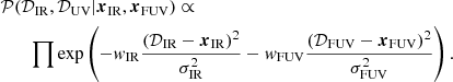 (A.2)
(A.2)
Summary of the parameters of the evolving, modified Schechter function and their priors.
The weights are derive to compensate the different number of data points available in FUV and IR, that is  and
and  .
.
We considered the modified Schechter function evolving with redshift, as reported in Eqs. (1) and (2), but we removed the extrapolation at z > 3 because FUV observations are available at higher redshifts. The G13 LF for AGN1 is considered a starting point for the MCMC chains.
In Fig. A.1 we report the corner plots, showing the correlation between the different parameters and the marginalised histogram of each parameter. All parameters show well-defined solutions and we report these in Table 1.
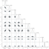 |
Fig. A.1. Corner plot of the MCMC performed considering simultaneously the FUV and IR data, contour lines are shown at arbitrary iso-density levels. Marginalised histograms are shown at the top of each column for each parameter. This plot has been derived using the Foreman-Mackey (2016) code. |
In Figs. A.2 and A.3, we show the result of the MCMC compared with the IR and FUV observations and the G13 IR LF for AGN2 and AGN1. The G13 IR LF of AGN1 describes the IR LF of AGN1 well, but overestimates the FUV LF of the same galaxy population. The new IR LF still describes the IR data, of both AGN1 and AGN2, but it also represents well the FUV LF of AGN1, with some discrepancies around z ∼ 2. This discrepancy may be due to the low number of SED templates associated with the AGN1 population in this work. In the future, increasing the number of SED templates may allow us to better sample the LIR-to-LFUV conversion.
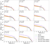 |
Fig. A.2. MCMC best result (solid green line) compared with AGN1 (black circles) and AGN2 (black squares) IR Herschel data and the AGN1 (dashed blue line) and AGN2 (dot-dashed magenta line) IR LF by G13. The orange lines are random extractions within 1σ uncertainty of the MCMC results. On the top left of each panel the average redshift and the χ2 are reported. |
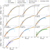 |
Fig. A.3. MCMC best result (solid green line) compared with the converted AGN1 IR LF by G13 (blue dashed line) and FUV observations (see legend). The orange lines are random extractions within 1σ uncertainty of the MCMC results. On the top left of each panel the average redshift and the χ2 are reported. |
Appendix B: Filters included in SPRITZ
In this appendix we report the complete list of filters included in the SPRITZ simulation. In particular, in Table B.1 we report the filter for which we derived absolute magnitudes. In the same table we also report the corresponding reference and the central wavelength of each filter, derived as follows:
 (B.1)
(B.1)
Filters included in the SPRITZ simulation to derive absolute magnitudes, their central wavelength, and the corresponding reference.
In Table B.2 we instead report the list of filters included in the SPRITZ simulation to derive the observed fluxes with their central wavelengths and the reference of each instrument.
Filters included in the SPRITZ simulation to derive observed fluxes, their central wavelength, and the corresponding reference.
All Tables
Parameters of the IR LFs used to derive the SPRITZ simulated galaxies, as found by G13 for Herschel galaxies or through the MCMC (for AGN1 and AGN2).
Parameters considered for smooth torus models (left) and clumpy torus models (right), as described in Sect. 2.2.1. Fritz et al. (2006), Feltre et al. (2012), and Nenkova et al. (2008a,b) provide further details.
IR emission features considered in the catalogue with the respective references: B19: Bonato et al. (2019), G16: Gruppioni et al. (2016), and M20: Mordini et al. (in prep.).
Recombination lines of the atomic hydrogen included in the SPRITZ simulation with the corresponding vacuum wavelengths (Lang 1999; Morton 2000).
Optical nebular emission lines included in the SPRITZ simulation for both star-forming systems and AGN.
Wavelength coverage and spectral resolution of the three spectrographs considered in SPRITZ.
Summary of the parameters of the evolving, modified Schechter function and their priors.
Filters included in the SPRITZ simulation to derive absolute magnitudes, their central wavelength, and the corresponding reference.
Filters included in the SPRITZ simulation to derive observed fluxes, their central wavelength, and the corresponding reference.
All Figures
|
Fig. 1. Workflow diagram summarising the main steps of SPRITZ. Orange coloured boxes indicate the outputs of the simulation. |
| In the text | |
|
Fig. 2. Spectral energy distribution templates used to derive SPRITZ simulated galaxies. Each panel shows templates of a specific galaxy population and all templates are normalised to the flux density at 5500 Å. |
| In the text | |
|
Fig. 3. Infrared LFs used in the SPRITZ simulation to derive simulated galaxies. Each panel shows a different galaxy population, as indicated on the top left. The LFs are shown for different redshifts from 0.1 (solid dark blue line) to 9.6 (solid dark red line) with steps of 0.5. At z > 3 we show the LFs derived assuming kΦ = −1 (see Eq. (2)) for all the populations except for AGN1 and AGN2 for which observations up to z = 5 are available. |
| In the text | |
|
Fig. 4. K-band LF used to include simulated elliptical galaxies in the SPRITZ simulation. The LFs are shown for different redshifts from 0.1 (solid dark blue line) to 4.6 (solid green line) with steps of 0.5, using the same colour code of Fig. 3. At z > 2 the LF has been extrapolated, starting from the Cirasuolo et al. (2007)K-band LF. |
| In the text | |
|
Fig. 5. Redshift evolution of the characteristic stellar mass M* (top) and characteristic density Φ* (bottom) of the GSMF of irregular galaxies. Data by Huertas-Company et al. (2016, black dots) and our fit (red solid line) are shown. The latter has been derived with the SCIPY package (Virtanen et al. 2020) and the resulting parameters are reported in each panel. |
| In the text | |
|
Fig. 6. GSMF used to include simulated irregular galaxies in the SPRITZ simulation. The GSMFs are shown for different redshifts from 0.1 (solid dark blue line) to 9.6 (solid dark red line) with steps of 0.5, with the same colour code as in Fig. 3. |
| In the text | |
|
Fig. 7. Comparison between the stellar mass (left), hydrogen column density (centre), and intrinsic X-ray luminosity (right) derived using SED3FIT with the clumpy and smooth torus library. All considered SED templates are scaled to have LIR = 1011 L⊙. Symbols indicate different galaxy populations: SF-AGN (dark-green circles), SB-AGN (orange squares), AGN type-1 (blue triangles), and AGN type-2 (magenta stars). In the central panel, empty symbols and arrows represent the upper limits to NH for the objects for which NH = 0 with one torus library, but not with the other torus library. These points are artificially set to log10(NH/cm−2 = −20.5 for visual purposes. We do not show objects for which NH = 0 using both torus libraries; this is comprised of three AGN1 templates and one SF-AGN template. The vertical dashed grey line indicates the maximum values of NH of the smooth torus library. Error bars indicate the 16% and 84% percentiles and, in the right panel, the scatter of 0.33 dex in the relation to derive X-ray luminosity (Asmus et al. 2015). The black dotted line in each panel indicates the identity line. |
| In the text | |
|
Fig. 8. Comparison between the X-ray luminosity obtained from the luminosity at 12 μm (Asmus et al. 2015) and the X-ray luminosity obtained from the AGN bolometric luminosity and assuming the correction by Duras et al. (2020). The comparison is shown separately for the smooth (top) and clumpy torus models (bottom). The different colours indicate the galaxy populations with an AGN component (see legend). The X-ray luminosities are compared before applying any dispersion and are shown for the smooth (top) and clumpy torus models (bottom). The dashed black line indicates the identity line while the dotted lines show the 1σ combined dispersion of the two relations. |
| In the text | |
|
Fig. 9. Comparison between the line luminosities derived using the relation by Bonato et al. (2019, B19, x-axis) with those derived with the relations by Gruppioni et al. (2016, blue solid lines) and Mordini et al. (in prep., red dashed lines). The contour lines indicate the 68%, 95%, and 99.7% percentiles of the distribution. The three panels show three different lines: PAH at 3.3 μm (left), [Ne V] 14.32 μm (centre), and [O I] 63.18 μm (right). The relations may be different for AGN and star-forming dominated systems, as explained in the text. |
| In the text | |
|
Fig. 10. Example of a low-resolution JWST/MIRI spectra of a SB-AGN galaxy at z = 2.88. At the top the rest-frame wavelengths are shown; on the bottom the observed wavelengths are shown. The original spectrum (solid black line), the spectrum after the addition of nebular lines (dashed red line), and the spectrum after the application of the spectral resolution and noise (dotted green line) are shown. On the top, short vertical dotted lines indicate the wavelength position of the nebular emission lines included despite their S/N. |
| In the text | |
|
Fig. 11. Example of a simulated field of 10′ × 10′. Each point represents a simulated galaxy and is colour coded depending on its redshift. |
| In the text | |
|
Fig. 12. Observed IR LFs derived in the ALPINE survey (black circles, Gruppioni et al. 2020) at z = 3.5 − 4.5 (top) and z = 4.5 − 6 (bottom). The empty circles are below the completeness limits. The ALMA IR LFs are compared with the four extrapolations of the total Herschel LFs used in this work to extract simulated galaxies at z > 3 (coloured solid lines). |
| In the text | |
|
Fig. 13. Differential number counts of the SPRITZ simulated galaxies from the U band to the near-IR with high-redshift extrapolation kΦ = −1 (Eq. (2), solid black line). The shaded regions show the uncertainties due to the high-z extrapolation and the 1σ errors of the LFs and GSMF used to generate simulated galaxies. Observations in the same bands of the CANDELS GOODS-S survey (filled circles, Guo et al. 20130 and data from the GAMA survey (filled squares, Hill et al. 2011) and the AKARI telescope (filled diamonds, Murata et al. 2014), both corrected for the differences in the broad-band filters, are also shown. For clarity, only one every four data points of the GAMA survey are shown. The dotted vertical black lines show a rough estimate of the 50% completeness level for CANDELS data. |
| In the text | |
|
Fig. 14. Differential number counts normalised to the Euclidean slope of the SPRITZ simulated galaxies in the mid- and far-IR with high-redshift extrapolation kΦ = −1 (Eq. (2), solid black line). The shaded regions show the uncertainties due to the high-z extrapolation and 1σ errors of the LFs and GSMF used to generate simulated galaxies. Several observed values present in the literature are also shown (Papovich et al. 2004; Le Floc’h et al. 2009; Clements et al. 2010; Berta et al. 2011; Béthermin et al. 2012, 2020; Pearson et al. 2012; Geach et al. 2013; Magnelli et al. 2013; Murata et al. 2014; Hsu et al. 2016; Valiante et al. 2016; Davidge et al. 2017; Geach et al. 2017; Wang et al. 2017; Zavala et al. 2017; Stach et al. 2018). The thin coloured lines represent the normalised number counts for the different galaxy populations considered in SPRITZ: spirals (light green line), SBs (cyan line), SF-AGN (dark-green line), SB-AGN (orange line), AGN type-1 (blue line), AGN type-2 (magenta line), elliptical galaxies (red line), and irregular galaxies (brown line). |
| In the text | |
|
Fig. 15. Stellar mass function of the SPRITZ simulation at different redshifts (thick solid black line), with high-redshift extrapolation kΦ = −1 (Eq. (2)) and −4 (thick dotted black line). The grey shaded area shows the uncertainties arising from the high-z extrapolation, the different torus library considered, the 1σ value derived from the probability distribution of the stellar mass of each SED template, and the 1σ errors of the LFs and GSMF used to derive simulated galaxies. Some of the values present in the literature are reported: Ilbert et al. (2013, green crosses), Davidzon et al. (2017, blue circles), Caputi et al. (2015, cyan squares) and Grazian et al. (2015, magenta triangles). The thin coloured lines represent the stellar mass functions for the different galaxy populations considered in SPRITZ: spirals (light green line), SBs (cyan line), SF-AGN (dark green line), SB-AGN (orange line), AGN type-1 (blue line), AGN type-2 (magenta line), elliptical galaxies (red line), and irregular galaxies (brown line). |
| In the text | |
|
Fig. 16. Stellar mass vs. SFR at different redshifts for simulated SPRITZ galaxies with high-redshift extrapolation kΦ = −1 (Eq. (2)). Blue shows the distribution of galaxies derived from the IR LF or the irregular GSFM, while red indicates the distribution of elliptical galaxies derived from the K-band LF. The colour gradients show the number of galaxy in 1 deg2 and these are in logarithmic scale, as shown on the right for star-forming galaxies (top colour bar) and ellipticals (bottom colour bar). The different lines show the observed position of normal star-forming galaxies as derived by Elbaz et al. (2011, dash-dot-dot-dotted green line), Speagle et al. (2014, dotted black line), Caputi et al. (2017, dash-dot-dotted yellow line), Santini et al. (2017, dash-dotted light green line), Bisigello et al. (2018, dashed orange line), and the relation derived for SBs by Caputi et al. (2017, pink dash-dot-dotted lines) and Bisigello et al. (2018, magenta dashed lines). |
| In the text | |
|
Fig. 17. Luminosity function at 8 μm for all galaxies simulated with SPRITZ (solid black tick line), with high-redshift extrapolation kΦ = −1 (Eq. (2)). The grey area shows the uncertainties due to the high-z extrapolation and 1σ errors of the GSFM, IR, and K-band LFs used to generate simulated galaxies. The LF for the different sub-populations is also shown: spirals (green line), SBs (cyan line), the two composite populations SF-AGN (dark green line) and SB-AGN (orange line), AGN type-1 (blue line), AGN type-2 (magenta line), elliptical galaxies (red line), and irregular galaxies (brown line). The observed 8 μm LFs by Rodighiero et al. (2010, red squares), Caputi et al. (2007, blue circles), Goto et al. (2015, 2019, green triangles), and Magnelli et al. (2011, light blue stars) are also represented. |
| In the text | |
|
Fig. 18. Same as Fig. 17, but for the K-band LF. The observed K-band LFs are represented by Mortlock et al. (2017, red squares), Cirasuolo et al. (2007, blue circles), and Beare et al. (2019, green triangles) in the overlapping redshift bins. |
| In the text | |
|
Fig. 19. Same as Fig. 17, but for the B-band LF. The observed B-band LFs are represented by Fritz et al. (2014, red squares), Beare et al. (2015, blue circles), Dahlen et al. (2005, green triangles), Poli et al. (2003, magenta upside-down triangles), Gabasch et al. (2004, pink pentagon), and Marchesini et al. (2007, light blue stars) in the overlapping redshift bins. |
| In the text | |
|
Fig. 20. Same as Fig. 17, but for the LF at 1600 Å. Our simulation is compared with other data from the literature (see legend). |
| In the text | |
|
Fig. 21. Luminosity function at 2–10 keV for all AGN simulated with SPRITZ (solid black line) with high-redshift extrapolation kΦ = −1 (Eq. (2)) and for the sub-sample of AGN with log10(NH/cm−2) < 23 (dotted black line). The grey area shows the uncertainties due to the conversion from the L12 μm to L2 − 10 keV, the use of different torus models, and the 1σ errors of the IR LFs used to derive the simulated galaxies hosting an AGN. The LF for each different sub-population is also shown (see Fig. 17). The observed X-ray LFs by Wolf et al. (2021, purple star), Miyaji et al. (2015, cyan squares), Aird et al. (2010, red circles), Aird et al. (2015, green and orange triangles), and Vito et al. (2018, yellow diamonds) are reported. |
| In the text | |
|
Fig. 22. Rest-frame LF at 1.4 GHz for all galaxies simulated with SPRITZ (solid black tick line) with high-redshift extrapolation kΦ = −1 (Eq. (2)), taking into account only the luminosity originated from the star formation activity. The grey areas indicate the uncertainties due to the high-z extrapolation, the different torus models included, and the 1σ errors of the GSMF, IR, and K-band LFs used to generate simulated galaxies. The LF for each different sub-population is also shown (see Fig. 17). The observed 1.4 GHz LFs, limited to the star-formation activity, by Novak et al. (2017, red squares), Bonato et al. (2021, blue circles), Smolčić et al. (2009, green trangles), and Upjohn et al. (2019, orange stars) are represented. |
| In the text | |
|
Fig. 23. Same as Fig. 22, but for radio-loud AGN. The observed 1.4 GHz LFs of radio-loud AGN by Ceraj et al. (2018, red squares), Bonato et al. (2021, blue circles), Smolčić et al. (2017, green trangles), and Butler et al. (2019, orange diamonds) are shown. |
| In the text | |
|
Fig. 24. BPT diagram for simulated galaxies. Data points are colour coded depending on the fraction of AGN measured in the IR. The solid black line shows the separation between AGN and H II region, as derived by Kewley et al. (2013b) at z ≤ 2.5. The dashed black line indicates the extrapolation of the same separation criteria at high reshifts. |
| In the text | |
|
Fig. 25. Redshift distribution (top) and stellar mass vs. redshift (bottom) of the simulated galaxies obtained with the SPRITZ simulation for the JWST JADES-Deep survey, considering only galaxies brighter than mAB, F150W = 30.6. The different colours indicate different galaxy populations, as listed in the legend. On the top, the grey shaded area indicates uncertainties due to the high-z extrapolation of the different LFs. |
| In the text | |
|
Fig. 26. Example of a NIRCam pointing in three filters: F090W (blue), F277W (green), and F44W (red). |
| In the text | |
|
Fig. 27. Redshift distribution (top) and LIR vs. redshift (bottom) of the OST simulated catalogues covering 500 deg2. Galaxies detected in both photometric filters, that is the band centred at 50 μm (left) and that centred at 250 μm (right), are represented. The different colours indicate different galaxy populations, as listed in the legend. On the top, the grey shaded area indicates uncertainties due to the high-z extrapolation of the different LFs. |
| In the text | |
|
Fig. A.1. Corner plot of the MCMC performed considering simultaneously the FUV and IR data, contour lines are shown at arbitrary iso-density levels. Marginalised histograms are shown at the top of each column for each parameter. This plot has been derived using the Foreman-Mackey (2016) code. |
| In the text | |
|
Fig. A.2. MCMC best result (solid green line) compared with AGN1 (black circles) and AGN2 (black squares) IR Herschel data and the AGN1 (dashed blue line) and AGN2 (dot-dashed magenta line) IR LF by G13. The orange lines are random extractions within 1σ uncertainty of the MCMC results. On the top left of each panel the average redshift and the χ2 are reported. |
| In the text | |
|
Fig. A.3. MCMC best result (solid green line) compared with the converted AGN1 IR LF by G13 (blue dashed line) and FUV observations (see legend). The orange lines are random extractions within 1σ uncertainty of the MCMC results. On the top left of each panel the average redshift and the χ2 are reported. |
| In the text | |
Current usage metrics show cumulative count of Article Views (full-text article views including HTML views, PDF and ePub downloads, according to the available data) and Abstracts Views on Vision4Press platform.
Data correspond to usage on the plateform after 2015. The current usage metrics is available 48-96 hours after online publication and is updated daily on week days.
Initial download of the metrics may take a while.