| Issue |
A&A
Volume 689, September 2024
|
|
|---|---|---|
| Article Number | A125 | |
| Number of page(s) | 16 | |
| Section | Extragalactic astronomy | |
| DOI | https://doi.org/10.1051/0004-6361/202450529 | |
| Published online | 06 September 2024 | |
Disentangling the co-evolution of galaxies and supermassive black holes with PRIMA
1
INAF, Istituto di Radioastronomia, Via Piero Gobetti 101, 40129 Bologna, Italy
2
Dipartimento di Fisica e Astronomia “G. Galilei”, Università di Padova, Via Marzolo 8, 35131 Padova, Italy
3
INAF-Osservatorio di Astrofisica e Scienza dello Spazio, Via Gobetti 93/3, 40129 Bologna, Italy
4
Department of Astronomy, University of Maryland, College Park, MD 20742, USA
5
Aix Marseille Univ., CNRS, CNES, LAM, Marseille, France
6
Department of Astronomy, University of Massachusetts, Amherst, MA 01003, USA
7
IPAC, California Institute of Technology, 1200 E. California Boulevard, Pasadena, CA 91125, USA
8
Ritter Astrophysical Research Center, University of Toledo, Toledo, OH 43606, USA
9
Center for Computational Astrophysics, Flatiron Institute, 162 5th Ave, New York, NY 10010, USA
10
Space Telescope Science Institute, 3700 San Martin Dr., Baltimore, MD 21218, USA
11
Department of Physics, University of Helsinki, Gustaf Hällströmin katu 2, 00014 Helsinki, Finland
12
NASA Goddard Space Flight Center, Greenbelt, MD 20771, USA
13
NASA Jet Propulsion Laboratory, 4800 Oak Grove Dr, Pasadena, CA 91011, USA
14
California Institute of Technology, 1200 E California Blvd, Pasadena, CA 91125, USA
15
INAF-Osservatorio Astrofisico di Arcetri, Largo E. Fermi 5, 50125 Firenze, Italy
Received:
26
April
2024
Accepted:
31
May
2024
The most active phases of star formation and black hole accretion are strongly affected by dust extinction, making far-infrared (FIR) observations the best way to disentangle and study the co-evolution of galaxies and super massive black holes. The plethora of fine-structure lines and emission features from dust and ionised and neutral atomic and warm molecular gas in the rest-frame mid-infrared (MIR) and FIR provide unmatched diagnostic opportunities to determine the properties of gas and dust, measure gas-phase metallicities, and map cold galactic outflows in even the most obscured galaxies. By combining multi-band photometric surveys with low- and high-resolution FIR spectroscopy, the PRobe far-Infrared Mission for Astrophysics (PRIMA), a 1.8 m diameter, cryogenically cooled FIR observatory currently at the conception stage, will revolutionise the field of galaxy evolution by taking advantage of this IR toolkit to find and study dusty galaxies across galactic time. In this work, we make use of the phenomenological simulation SPRITZ and the Santa Cruz semi-analytical model to describe how a moderately deep multi-band PRIMA photometric survey can easily reach beyond previous IR missions to detect and study galaxies down to 1011 L⊙ beyond cosmic noon and at least up to z = 4, even in the absence of gravitational lensing. By decomposing the spectral energy distribution (SED) of these photometrically selected galaxies, we show that PRIMA can be used to accurately measure the relative AGN power, the mass fraction contributed by polycyclic aromatic hydrocarbons (PAHs), and the total IR luminosity. At the same time, spectroscopic follow up with PRIMA will allow us to trace both the star formation and black hole accretion rates (SFRs and BHARs), the gas-phase metallicities, and the mass-outflow rates of cold gas in hundreds to thousands of individual galaxies to z = 2.
Key words: surveys / galaxies: active / galaxies: evolution / galaxies: photometry
© The Authors 2024
 Open Access article, published by EDP Sciences, under the terms of the Creative Commons Attribution License (https://creativecommons.org/licenses/by/4.0), which permits unrestricted use, distribution, and reproduction in any medium, provided the original work is properly cited.
This article is published in open access under the Subscribe to Open model. Subscribe to A&A to support open access publication.
1. Introduction
Supermassive black holes (SMBHs) of millions of solar masses seem to be ubiquitous at the centre of galaxies in the local Universe (e.g. Magorrian et al. 1998; Gültekin et al. 2009; McConnell et al. 2011). Observations have pointed out the presence of relations between the mass of the SMBH and many properties of the host galaxy, such as the stellar mass and the velocity dispersion of the galaxy bulge (Magorrian et al. 1998; Ferrarese 2002), the halo mass (e.g. Ferrarese 2002), and the stellar mass of the host itself (e.g. Mullaney et al. 2012; Reines & Volonteri 2015). The presence of these scaling relations suggests a close evolutionary link between the SMBH and its host galaxy (Kormendy & Ho 2013).
Co-evolution between SMBHs and their host galaxies is also supported by the similarity between the time evolution of the cosmic star-formation-rate density (SFRD; e.g. Gruppioni et al. 2013; Madau & Dickinson 2014; Traina et al. 2024) and that of the black-hole accretion rate density (BHARD; e.g. Delvecchio et al. 2014). Indeed, both quantities show an increase from early epochs up to z ∼ 2 − 3, followed by a rapid decrease; although these measures are made from disjoint samples. While the rough shape of the SFRD with cosmic time can be understood in the context of merger-driven evolution, theoretical models calibrated to reproduce present-day scaling relations seem to produce a wide range in the BHARD at higher redshifts (Habouzit et al. 2020, 2021) due to differences in the implementation of supernova and black hole feedback and subgrid physics.
Observationally, the study of both the SFRD and the BHARD is hampered by the presence of dust, as the most active phases of black hole growth and star formation (SF) are heavily enshrouded. Indeed, the contribution of the dust-obscured SFRD to the total is above 50% at least up to z = 4 (Zavala et al. 2021; Traina et al., in prep.). Moreover, some galaxies are so obscured by dust that they are detectable in the infrared (IR) but are faint or totally missed at optical wavelengths (e.g. Gruppioni et al. 2020; Talia et al. 2021; Rodighiero et al. 2023; Bisigello et al. 2023; Pérez-González et al. 2023).
Herschel results showing that the majority of IR galaxies with LIR > 1011 L⊙ at z > 1 host a low-luminosity or obscured AGN (AGN; Gruppioni et al. 2013; Magnelli et al. 2013) support the hypothesis of co-growth and co-evolution of SMBHs and galaxies, highlighting the need to observe the peak of their activity (i.e. cosmic noon) in the IR. Similarly, recent James Webb Space Telescope (JWST) observations of numerous faint, broad-line AGN at z > 5 (e.g. Onoue et al. 2023; Kocevski et al. 2023; Harikane et al. 2023; Larson et al. 2023) may point to Eddington-limited accretion onto massive black hole seeds formed at z > 15 (e.g. Maiolino et al. 2023). At the same time, about 20% of the broad-line AGN identified with JWST appear as red and compact sources, with a steep red continuum in the rest-frame optical and a blue/flat continuum in the rest-frame ultraviolet (UV; e.g. Kocevski et al. 2023, 2024; Harikane et al. 2023; Matthee et al. 2024; Greene et al. 2024; Killi et al. 2023). Despite the AGN signature in the rest-frame optical, the majority of these so-called ‘little red dots’ are sources of weak or undetected X-ray emission with Chandra (Yue et al. 2024). These objects could be heavily obscured by dust heated by buried AGN (e.g. Kocevski et al. 2023; Matthee et al. 2024; Greene et al. 2024), very compact starbursts with large numbers of OB stars (e.g., Pérez-González et al. 2024), Compton-thick AGN with a dust-poor medium, or intrinsically X-ray-weak AGN, such as narrow line Seyfert 1s (Maiolino et al. 2024).
Given the observational and theoretical evidence that galaxies and their SMBH grow together, and that the most rapid growth occurs during phases that are hidden by dust (Hickox & Alexander 2018), it is essential to measure SFR and BHAR in high-z populations using tools that are insensitive to the effects of dust obscuration. It is also important to perform these studies in the same populations of galaxies, where observation biases can be well understood and selection effects minimised. The rest frame mid- and far-infrared (MIR and FIR, respectively) spectrum offers a plethora of fine-structure gas lines and emission features from dust and warm molecular gas that are sensitive to AGN and SF activity (Fig. 1) and are not (or very little) affected by dust extinction. In particular, among the AGN tracers, there are [Ne V] at 14.3 and 24.3 μm, [O IV] at 24.9 μm, and [Ne III] at 15.7 μm (e.g. Rigby et al. 2009; Fernández-Ontiveros et al. 2016; Feltre et al. 2023). At the same time, polycyclic aromatic hydrocarbon (PAH) emission features present between 3 and 20 μm; the MIR pure rotational lines of H2 at 17 μm; and the low-ionisation fine-structure lines, such as the [Ne II] line at 12.8 μm, the [S III] lines at 18 and 33 μm, and the [C II] line at 158 μm (e.g. De Looze et al. 2014; Vallini et al. 2015) are sensitive tracers of SF. While some of these lines are excited by both SF and AGN activity, it has been shown that the relative contributions can be decomposed (Stone et al. 2022). Many of these lines have already been used in the local Universe to study the SFR and the BHAR in individual bright IR galaxies (e.g. Armus et al. 2004, 2006, 2007, 2023; Spinoglio et al. 2015, 2022; Spoon et al. 2009; Díaz-Santos et al. 2013; Inami et al. 2013; Stierwalt et al. 2014; Lai et al. 2022; Stone et al. 2022), but cold-sensitive FIR observatories are necessary to extend these studies to higher redshifts and to less extreme galaxies.
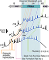 |
Fig. 1. Example of MIR and FIR spectra of galaxies. The spectra at these wavelengths contain a plethora of features useful for deriving SFR, BHAR and metallicity. The observed wavelengths of some of these tracers are reported in the figure, together with the SED of an example star-forming galaxy at z = 0, z = 2, and z = 4 taken from Moullet et al. (2023, Section 47). We also highlight the wavelength coverage of JWST, PRIMA (shaded region), and ALMA. |
Dust grains play a crucial role in the formation and cooling of molecular gas and therefore in the formation of new stars (Draine 2003; Peimbert & Peimbert 2010). For this reason, theoretical models predict that the dust abundance and metallicity of the interstellar medium (ISM) should be closely related (Zhukovska 2014), as large fractions of metals are converted into dust when they are injected into the ISM by asymptotic giant branch stars and supernovae. At the same time, the rate of dust destruction by supernova blast waves is thought to be an order of magnitude higher than dust production by dying stars (Dwek & Cherchneff 2011). There is clearly a large gap in our knowledge of dust formation (and SF as a consequence) and destruction, which can be solved only by tracing both metals and dust in the same galaxies. PAHs features, present in the rest-frame MIR, are known to be tracers of SF, but they are also sensitive tracers of the abundance of small carbonaceous dust grains. At the same time, in dusty galaxies, gas metallicity can be measured using bright FIR tracers such as [N III]57 μm, [O III]52 μm, and [O III]88 μm (Nagao et al. 2011; Pereira-Santaella et al. 2017; Fernández-Ontiveros et al. 2017), which are unaffected by dust extinction and have a negligible dependence on the gas temperature, unlike their optical and UV counterparts (e.g. Bernard Salas et al. 2001).
To fully understand the interplay between AGN and their host galaxies, it is also necessary to identify and measure galactic outflows, a powerful form of feedback that can inject significant amounts of energy into the ISM, and drive gas and dust into the circumgalactic medium (CGM). Outflows are invariably multi-phase, but the cold (T < 104 K) component often dominates the gas mass (Veilleux et al. 2020). Spectroscopic observations of strong absorption features in the FIR, such as OH, can be used to estimate the outflow velocity and mass outflow rate (González-Alfonso et al. 2014, 2017). Observations of cold outflows using OH absorption lines have been very effective, indicating large masses of outflowing dense gas that can rival or exceed the star formation rate (SFR) in ultraluminous IR galaxies (González-Alfonso et al. 2017). Nevertheless, detailed studies have so far been limited to small numbers of galaxies in the Local Universe (see Veilleux et al. 2020, for a review). Sensitive, cold FIR spectroscopic observatories that can reach significantly fainter levels than were possible with Herschel are necessary to extend these studies to high redshifts and trace cold outflows to cosmic noon and beyond in statistically significant samples of normal galaxies.
The PRobe far-Infrared Mission for Astrophysics, PRIMA1 (PI: J. Glenn), is a cryogenically cooled FIR observatory with a diameter of 1.8 m, presently in the concept stage. PRIMA’s current design includes two science instruments: FIRESS and PRIMAger. FIRESS is a powerful, multi-mode survey spectrometer covering wavelengths between 24 and 235 μm with two different spectral modes: a low-resolution mode with R ∼ 100 and a high-resolution FTS mode, which offers tunable spectral resolution up to R = 4400 at 112 μm and 20 000 at 25 μm. PRIMAger is a multi-band spectrophotometric imager that offers hyperspectral linear variable filters in two bands (R = 10, PHI1 and PHI2) from 24 to 80 μm together with polarimetric capabilities in four broadband filters (PPI) between 80 and 261 μm. Because it is cooled, and uses state-of-the-art kinetic inductance detectors (e.g. Day et al. 2003, 2024; Baselmans 2012), PRIMA is orders of magnitude more sensitive than previous FIR space missions. PRIMA is designed to rapidly survey the IR sky, achieving mapping speeds 3−5 orders of magnitude faster than its FIR predecessors. In this work, we outline the revolutionary role that PRIMA will play in studying galaxy and AGN co-evolution across cosmic time. Although here we illustrate the power of PRIMA by describing possible deep and wide surveys and follow-up spectroscopy with PRIMAger and FIRESS, we must stress that PRIMA is a true community observatory, with at least 75% of the observing time available to astronomers through a traditional, peer-reviewed, ‘general observers’ program (for an overview of different general observer science cases, see Moullet et al. 2023). Moreover, all PI data will be publicly available to guest investigators.
The paper is organised as follows. In Sect. 2 we present the PRIMA example surveys together with the simulations used in the analysis. In Sect. 3 we discuss the SFR, BHAR, metallicity, and outflow measurements using both photometric and spectroscopic IR observations. We finally report and summarise our conclusions in Sect. 4. Throughout the paper, we consider a ΛCDM cosmology with H0 = 70 km s−1 Mpc−1, Ωm = 0.27, and ΩΛ = 0.73, and a Chabrier initial mass function (IMF, Chabrier 2003).
2. Methods
To assess the capability of PRIMA to disentangle galaxy and AGN evolution as well as to measure metallicity and cold outflows, we made use of the spectrophotometric realisations of IR-selected targets at all-z (SPRITZ2 v1.13; Bisigello et al. 2021, 2022) and the Santa Cruz semi-analytic model (SC SAM; Somerville et al. 2015). In the following sections, we provide some brief details of the PRIMAger instrumental capabilities and of these two simulations, and explain how it is possible to measure both SFR and BHAR using FIR spectrophotometric data.
2.1. PRIMA surveys
As example cases, we considered two different designs for the PRIMAger surveys. Both surveys have a total observing time of 1500 h, which are distributed over 1 deg2 for the Deep survey and over 10 deg2 for the Wide survey. In the remainder of the paper, we consider a galaxy as detected if it has a S/N > 5 in half of the PRIMAger hyper-spectra filters (PHI). This ensures a good description of the overall FIR SED and limits problems due to source confusion. Table 1 lists the PRIMAger filters and the depths considered for the Deep and Wide surveys. As a reference, we use the conservative depths, taking into account that current best estimate (CBE) for the instrument is better than this conservative expectation by a factor of ∼1.7 in the hyper-spectra PHI bands and ∼2 in the long wavelengths PPI filters. However, when necessary, we also make a comparison with the payload limits, which are the guaranteed requirement payload depths. Although the hyper-spectra filter PHI band of PRIMAger will provide continuous, highly over-sampled spectra at R = 10 from 24 to 80 μm, we assume in the following that this band is composed of 12 top-hat filters with R = 10. Similarly, we represent the four PRIMAger broad band filters (PPI) as continuous rectangular filters spanning the wavelength range of the band; that is, R = 4.
PRIMAger filter bandpasses and survey depths.
From these photometric surveys, it will be possible to select a subsample of sources to follow-up spectroscopically with FIRESS. In particular, with one hour of integration time, we expect to detect lines with fluxes above 10−19 W/m2 with the low-resolution mode of FIRESS. As shown in Fig. 2, we expect the number of observed spectroscopic sources to be well below the limit of 15 sources per beam per resolution element, above which we expect PRIMA could be affected by line confusion. We note that these line counts do not include the effects of photometric confusion, which could increase line blending in some cases. However, at the depth of 10−19 W/m2, FIRESS should not be largely affected by line confusion, even at the longest observed wavelength (i.e. 235 μm). This is true even down to a depth of 10−20 W/m2.
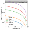 |
Fig. 2. Cumulative line number counts per beam and resolution element. Numbers are shown at different wavelengths, as derived using SPRITZ. We do not expect FIRESS to be affected by line confusion down to at least 10−20 W/m2. The vertical dotted line shows the flux of 10−19 W/m2, reachable with FIRESS with one hour of integration time. The horizontal dashed line and the shaded region show the limit of 15/beam/R, above which PRIMA could be affected by line confusion at the longest wavelengths. |
2.2. SPRITZ
The SPRITZ simulation is particularly well suited to making predictions for PRIMA as it starts from previously observed IR luminosity functions (Gruppioni et al. 2013) of star-forming galaxies, AGN, and composite systems. These are complemented with the K-band luminosity function of elliptical galaxies and the galaxy stellar mass function of dwarf irregular galaxies. These functions are used in SPRITZ to derive the number of galaxies expected at different redshifts (z = 0 − 10) and IR luminosities ( ). The galaxies included in the simulations can be broadly grouped into four populations:
-
Star-forming galaxies correspond to star-forming galaxies with no evident sign of AGN activity. This class includes spiral galaxies and starbursts as derived from the observed Herschel IR luminosity functions (Gruppioni et al. 2013), and dwarf irregular galaxies as derived from their observed galaxy stellar mass function (Huertas-Company et al. 2016; Moffett et al. 2016). Spiral galaxies have specific star-formation rates log(sSFR/yr−1) = − 10.4 to −8.9, while starbursts have higher sSFRs ranging from log(sSFR/yr−1) = − 8.8 to −8.1. Dwarf irregular galaxies are instead those with lower stellar masses, as their characteristic stellar mass (i.e. mass at the knee of the mass function) is log10(M*/M⊙)≤11.
-
AGN-dominated systems are galaxies whose MIR emission is dominated by AGN activity. These include two different populations, which differ in terms of their optical extinction, namely AGN1 and AGN2. Their number densities were derived by Bisigello et al. (2021), who combined the observed AGN IR and UV observed luminosity functions (Gruppioni et al. 2013; Croom et al. 2009; McGreer et al. 2013; Ross et al. 2013; Akiyama et al. 2018; Schindler et al. 2019).
-
Composite systems are objects whose energetics are dominated by SF, but which include a faint AGN component. These are split into star-forming AGN (SF-AGN), which have an intrinsically faint AGN (i.e. Lbol ≤ 1013 L⊙), and SB-AGN, whose AGN is bright but extremely obscured (i.e. log(NH/cm−2) = 23.5 − 24.5). Both populations are derived starting from the observed Herschel luminosity function (Gruppioni et al. 2013).
-
Passive galaxies are elliptical galaxies, generally with little or no SF, as derived from the observed K-band luminosity functions (Arnouts et al. 2007; Cirasuolo et al. 2007; Beare et al. 2019). Some of these galaxies may host an obscured AGN.
To each simulated galaxy we assign one SED model that depends on its galaxy population (Polletta et al. 2007; Rieke et al. 2009; Gruppioni et al. 2010; Bianchi et al. 2018) in order to derive the photometric fluxes expected in different filters, spanning from UV to radio wavelengths. The proportions of galaxies belonging to each population is derived by the luminosity function evolution of the different galaxy classes, at different redshifts and luminosities. We then fit the empirical SED assigned to each simulated galaxy using the software SED3FIT (for AGN; Berta et al. 2013), in order to disentangle the AGN from the galaxy contribution, or the software ‘multi-wavelength analysis of galaxy physical properties’ (MAGPHYS; for non-active objects; da Cunha et al. 2008). From the fit, we retrieved the stellar mass, the accretion luminosity, the hydrogen column density of the dusty torus, and the contributions to the IR luminosity of SF and AGN activity. The SFR is directly taken from the UV continuum and the IR luminosity for the unobscured and obscured components, respectively. We then used several theoretical and empirical relations to derive additional physical properties, which are marginally or not constrained from the SED fitting, such as the X-ray AGN luminosity and the metallicity.
The simulation also includes IR emission lines due to SF or AGN activity associated to the SEDs through several empirical relations (e.g. Bonato et al. 2019; Gruppioni et al. 2016). In the following section, we report some update required to take into account the dependence of some key IR lines on metallicity.
Overall, SPRITZ is consistent with a large set of observations from z = 0 to z = 6. This includes luminosity functions and number counts at different redshifts from X-rays to radio, the total galaxy stellar mass function, the molecular gas mass density, the CO and [CII] luminosity functions (Bisigello et al. 2022), AGN diagnostic diagrams (Euclid Collaboration 2024), and the SFR versus stellar mass plane. We refer to Bisigello et al. (2021, 2022) and (Euclid Collaboration 2024) for further comparisons with observations and more details on the SPRITZ simulation.
2.2.1. Linking FIR lines to gas metallicity in SPRITZ
Rest frame MIR and FIR emission lines are included in the SPRITZ simulation using the empirical relations by Bonato et al. (2019) and Gruppioni et al. (2016), linking the line luminosity to LIR. However, future IR facilities, such as PRIMA, with sensitive spectral capabilities can take advantage of metal-sensitive FIR lines including [N III]57 μm, [O III]52 μm, and [O III]88 μm to trace gas metallicity. For this reason, we implement an alternative approach to estimate the strengths of these key FIR lines in the galaxies modelled with SPRITZ.
As demonstrated by Lamarche et al. (2022), the absolute O/H abundance can be derived directly from measurements of the FIR cooling lines [O III]52 μm and/or [O III]88 μm, when supplemented with a tracer of hydrogen emission measure (recombination or free-free emission). The relative abundance measure N/O is also of particular interest, because nitrogen undergoes enhancement relative to oxygen from secondary production in CNO cycle stars. The N/O abundance has been established to correlate well with absolute abundance locally (Nagao et al. 2011; Pereira-Santaella et al. 2017; Spinoglio et al. 2022), revealing significant discrepancies with optical abundance measure in dusty local systems (Peng et al. 2021; Chartab et al. 2022).
To incorporate realistic luminosities for abundance-sensitive lines, we start by incorporating the [O III]88 μm line using the analytical model by Yang & Lidz (2020), which links the [O III]88 μm luminosity directly to the gas metallicity (Z) and the SFR:
![$$ \begin{aligned} \frac{L_{[{\text{O}}{\small {{\text{ III}}}}]88\,\upmu \mathrm{m}}}{L_{\odot }}=10^{8.27-0.0029\,(7.3+\log (Z/Z_{\odot }))^{2.5}}\,\frac{Z}{Z_{\odot }}\,\frac{\mathrm{SFR}}{M_{\odot }/\mathrm{yr}}, \end{aligned} $$](/articles/aa/full_html/2024/09/aa50529-24/aa50529-24-eq2.gif)
where Z⊙ indicates the solar value.
The ratio between the [O III]52 μm and [O III]88 μm line is a strong function of the electron density ne (e.g. Draine 2011). In SPRITZ, we randomly assign an electron density ne between 102 and 103 cm−3 to each galaxy and derive the [O III]52 μm expected luminosity directly from the [O III]88 μm luminosity. These electron densities are consistent with measurements obtained using MIR and FIR density-sensitive tracers in local Universe systems spanning moderate to very high specific SFRs (e.g. Dale et al. 2006; Inami et al. 2013; Herrera-Camus et al. 2016).
From the metallicity and the respective oxygen abundance, we retrieved the expected nitrogen abundance, as quantified in the local Universe using observations of late-type galaxies by Pilyugin et al. (2014):
We then made use of this information to estimate the nitrogen-to-oxygen-abundance ratio (N/O). This allowed us to predict the [N III]57 μm luminosity from the [O III]52 μm line, assuming an electron density of 104 cm−3 (near the critical density of both lines) and a temperature of 104 K:
![$$ \begin{aligned} \frac{L_{[{\text{N}}{\small {{\text{ III}}}}]57\,\upmu \mathrm{m}}}{L_{[{\text{O}}{\small {{\text{ III}}}}]52\,\upmu \mathrm{m}}}=\frac{\mathrm{N}}{\mathrm{O}}\,\frac{1}{0.4}\,\frac{1.0+0.377\,x+0.0205\,x^{2}}{1.0+0.691\,x+0.0966\,x^{2}}, \end{aligned} $$](/articles/aa/full_html/2024/09/aa50529-24/aa50529-24-eq4.gif)
where  (Peng et al. 2021).
The above methods allow us to derive the line luminosity powered by stellar activity; however, all three lines can also be powered by AGN activity. In order to include this contribution, we used the models from Feltre et al. (2016), computed with the photoionisation code CLOUDY (v13.03, Ferland et al. 2013). In particular, we consider an ionisation parameter at the Strömgren radius randomly varying between log10(US) = −1.5 and −3.5, a range of sub- and supersolar interstellar metallicity (0.008, 0.017, 0.03), a UV spectral index of α = −1.4, a dust-to-metal ratio of 0.3 and an internal microturbulence velocity of v = 100 km/s (see Mignoli et al. 2019). The hydrogen number density is assumed to be 103 cm−3.
Figure 3 shows the comparison between these line flux estimates and the empirical relation presented in Bonato et al. (2019). The estimates for [O III]52 μm and [O III]88 μm are largely consistent with the empirical relations. However, the estimated [N III]57 μm line luminosity, while consistent for AGN and composite objects, is on average around 1 dex below the empirical relation for purely star-forming objects. Nevertheless, these line luminosities are well below the luminosity range traced by the observations used by Bonato et al. (2019). Similar results, although with a larger scatter, are obtained if we consider the line luminosities obtained using the empirical relations by Gruppioni et al. (2016). We therefore conclude that, for the purposes of predicting PRIMA detection rates, the estimated line luminosities of [O III]52 μm, [O III]88 μm, and [N III]57 μm in SPRITZ used here, which include a realistic dependence on metallicity, are generally consistent with previous observations.
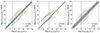 |
Fig. 3. Metallicity-dependent method outlined in Sect. 2.2.1. This method provides luminosity estimates consistent with those derived using the empirical relations by Bonato et al. (2019). In the figure we show the comparison for the [O III]52 μm (left), [N III]57 μm (centre), and [O III]88 μm (right) lines. Dotted lines indicate a 1:1 relation, with the shaded region showing the 1σ of the relations by Bonato et al. (2019). The vertical dashed lines show the minimum line luminosity used in the relation by Bonato et al. (2019). Contours correspond to 68%, 95%, and 99.7% of the distribution of objects hosting an AGN (orange dashed contours) and non-active galaxies (solid blue contours). |
2.3. Santa Cruz SAM
In addition to SPRITZ, we make also use of the state-of-the-art Santa Cruz semi-analytic model (SC SAM Somerville et al. 2015). For the purpose of this work, we used five simulated past lightcones presented by Yung et al. (2023), each covering an area of 2 deg2 and spanning a redshift range of 0 < z ≲ 10. These lightcones are constructed with halos extracted from the dark matter-only cosmological SMDPL simulation from the MultiDark suite, which has a volume of (400 Mpc h−1)3 and reliably resolves halos down to Mh ∼ 1010 M⊙ (Klypin et al. 2016). For halos in a lightcone, Monte Carlo realisations of dark-matter-halo merger histories are constructed using an extended Press-Schechter (EPS)-based algorithm (e.g. Somerville & Kolatt 1999), which provides input for the SC SAM described below. We refer the reader to Yung et al. (2022) and Somerville et al. (2021) for details regarding the constructions of lightcones.
The galaxies and AGN in the lightcones are simulated with the versatile and well-established SC SAM (Somerville & Primack 1999; Somerville et al. 2008, 2015), which models the formation and evolution of large ensembles of galaxies by tracking the flows of mass and metals into and out of the intergalactic medium, galaxy halos, and galaxies. These flows are driven by physical processes occurring across a vast range of scales, including gas accretion from the cosmic web into halos, cooling from the CGM into cold gas reservoirs within galaxies, BH accretion in the centres of galaxies, and large-scale galactic outflows driven by supernovae and AGN feedback. The SAM provides predictions for a wide range of physical properties, including stellar mass, SFR, black hole mass, and BHAR (Somerville et al. 2021; Yung et al. 2019a). The simulated galaxy populations in the lightcones are complete down to M* ∼ 107 M⊙. With physical parameters calibrated to a subset of observed galaxy properties at z ∼ 0, the SAM is able to reproduce the evolution of many observational quantities, including multi-wavelength luminosity functions up to z ∼ 10, one-point distribution functions of stellar mass and SFR up to z ∼ 8, and various scaling relations (Somerville et al. 2015, 2021; Yung et al. 2019a,b). The spatial distribution of sources in the lightcone are in excellent agreement with the observed two-point angular correlation functions (Yung et al. 2022). In addition, the model has also been shown to reproduce the observed evolution in AGN bolometric, UV, and X-ray luminosity functions up to z ∼ 5 (Hirschmann et al. 2012; Yung et al. 2021).
2.4. Deriving SFR and BHAR from FIR spectrophotometric data
Spectral energy distributions that extend from approximately 15 μm to 150 μm in the rest frame can be used to reliably determine the respective importance of SF and black hole accretion activity (Kirkpatrick et al. 2015; Ciesla et al. 2015; Gruppioni et al. 2015), as shown in Fig. 4. This tends to work because the AGN contributes primarily to warm dust that emits in the rest frame MIR range peaking around 20 μm, while SF activity creates a colder dust component that dominates the FIR, peaking around 100 μm (Shimizu et al. 2017).
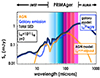 |
Fig. 4. Example of SED decomposition for an LIR = 1012 galaxy at z = 2. Star formation-(blue) and AGN-heated dust (orange) are shown schematically here and combine to produce a composite galaxy SED (black) that can be decomposed using the PRIMAger bands, shown here in different colours, from pale blue to magenta. |
Studies based on SED decomposition show that the warm dust temperature, the colour temperature, and the relative luminosity of the cold and warm components are all excellent indicators of the fraction of power contributed by the AGN in the MIR and bolometrically (Kirkpatrick et al. 2015). For highly obscured galaxies, such as those prevalent at z ∼ 1 − 2, dust luminosity is an excellent proxy for the bolometric luminosity of the system. Thus, the MIR luminosities of warm dust can be used to directly compute the bolometric luminosity of the AGN ( ). Indeed, as shown for example by (Gruppioni et al. 2016) and reported in Fig. 5 using a sample of local AGN, the AGN bolometric luminosity derived through SED fitting and decomposition is in very good agreement with the AGN bolometric luminosity derived from high-ionisation fine-structure lines, such as [O IV]26 μm. We note that for the data shown in the figure, a linear regression fit gives a slope of 0.9 ± 0.3 for the [O IV] versus SED-fit derivations, with the best-fit line crossing the 1−1 relation at Lbol(SED − fit)∼1010 L⊙. However, a more accurate analysis should be done on larger and complete samples in order to be used as calibration. On the contrary, X-rays tend to underestimate the AGN luminosity, particularly for highly obscured objects. Indeed, the X-ray bolometric corrections of Compton-thick AGN (empty stars in Fig. 5) derived by Brightman & Nandra (2011) using 2−10 keV X-ray observations increased once hard X-ray measurements became available (e.g. NuSTAR La Caria et al. 2019), moving
  closer to the estimation from SED fitting. The possibility that the absorption-corrected 2−10 keV luminosity (and consequently Lbol(X)) is underestimated for moderately obscured, Compton-thick AGN –if additional multi-wavelength data are not taken into account (e.g. SED-fitting)– has also been highlighted by Lanzuisi et al. (2015).
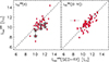 |
Fig. 5. Power of SED decomposition to derive the AGN bolometric luminosity ( |


Overall, these correlations demonstrate the potential use of SED decomposition to derive  for sources without MIR spectroscopy (i.e. too faint or high-z). Once the AGN bolometric luminosity is known, it is possible to compute the BHAR (through the standard assumption of 10% efficiency, Hopkins et al. 2007). Similarly, SFRs can be derived from the colder dust component visible in the FIR (blue curve in Fig. 4) using the standard relations derived for local galaxies (Kennicutt & Evans 2012) and bright lines such as [Ne II]13 μm (e.g. Spinoglio et al. 2022).
3. Results
The blending of sources due to the limited spatial resolution of FIR telescopes can be an important limitation to the ultimate attainable sensitivity in an observation. This limit is usually characterised by a so-called ‘confusion noise’, which corresponds to the level of the blended background of sources at a given wavelength and resolution. Recent work demonstrates that deblending techniques based on the Bayesian source extractor XID+ can be used to push below the classical confusion (the confusion limit reached by a basic blind source extractor) in PRIMAger (Donnellan et al. 2024) by leveraging the information provided by shorter wavelengths and the dense wavelength coverage of the instrument. In particular, Donnellan et al. (2024) show that a self-contained approach – based on using positional priors from a source catalogue detected in the shortest PRIMAger bands, with Wiener-filtering to deblend the longer PRIMAger wavelengths – can reach factors of 2 − 3 below the classical confusion limit. The use of a denser catalogue (e.g. obtained from Roman Space Telescope IR observations of the same field) together with weak intensity priors can push this limit even further, that is, to factors of 5 − 10 below the confusion limit at the longer wavelengths. Most importantly, Donnellan et al. (2024) show that the self-contained Wiener-filter catalogue approach allows PRIMAger to recover the SEDs of galaxies at the knee of the luminosity function at z = 2 out to PPI_2 (see their Figures 7 and 9). The calculations presented in the following sections use these results.
3.1. The galaxy population observed by PRIMAger
As shown in Fig. 6, using the conservative depths, we can detect galaxies with LIR > 1013 L⊙ up to z = 7 − 8 in both the deep and wide PRIMAger surveys. Less-extreme galaxies with luminosities down to LIR = 1011 L⊙ can be detected to z = 4 in the Deep survey and up to z = 3 in the Wide survey. As a comparison, with Herschel it was possible to observe galaxies with LIR = 1011 L⊙ only to z < 1 (e.g. Gruppioni et al. 2013; Magnelli et al. 2013). If we consider the payload depths, which are the minimal guaranteed depths, we lose 28% of galaxies in the Deep and 35% in the Wide survey; although in the latter, galaxies are limited to z = 6.5.
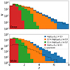 |
Fig. 6. Redshift distribution of galaxies observed by PRIMAger. The proposed PRIMAger surveys will not be limited to only the brightest IR galaxies. We show the number of galaxies as a function of redshift for the Deep (top, 1500 h/deg2) and Wide (bottom, 150 h/deg2) surveys using the SPRITZ simulation. We consider only galaxies with S/N ≥ 5 in at least 6 out of 12 PRIMAger Hyperspectra filters (i.e. PHI1–PHI2 in Table 1). The black solid lines show the total redshift distributions considering the payload depths. |
To understand the physical properties of these photometric samples, we present in Fig. 7 the SFR as a function of redshift for both the Deep and the Wide PRIMAger surveys. Using the conservative depths, we expect the Deep survey to be 50% complete for star-forming galaxies with stellar masses of log(M*/M⊙) = 10.5 and 11.5 up to z = 2.3 and z = 4, respectively. We note that for galaxies over log(M*/M⊙) = 10.5 at z ∼ 2, the study by Donnellan et al. (2024) shows that the SEDs are well measured over a large fraction of the bandpass using the XID+ deblending (see their Figure 9), and so we expect to be able to accurately measure their SFR and BHAR. The Wide survey should be 50% complete for galaxies with log(M*/M⊙) = 11.5 up to z = 2.9. Photometric surveys with PRIMAger would not be limited to the brightest, most luminous IR galaxies at z > 1, as was the case for previous FIR missions, but would finally start to also include a more representative sample of star-forming galaxies out to cosmic noon and beyond.
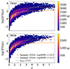 |
Fig. 7. Redshift and SFR of galaxies observed by PRIMAger. PRIMA surveys will not be limited to extremely bright objects, but will start to probe normal star-forming galaxies. We show the distribution of SFR as a function of redshift for the Deep (top) and Wide (bottom) surveys using the conservative depths (see Table 1) and the SPRITZ simulation. The cyan dashed lines indicate the 50% completeness level, while the orange solid and the dash-dotted lines show the SFR of a typical main sequence star-forming galaxy with log(M/M*) = 10.5 and log(M/M*) = 11.5, respectively. These were derived considering the M* − SFR relation by Speagle et al. (2014) at different redshifts. |
3.2. SFR versus BHAR with PRIMAger using the FIR continuum
As previously discussed, the rest-frame continuum between 15 and 150 μm can be used to disentangle the SF and black hole accretion activity, as the dust heated by these mechanisms has two different temperature distributions. In the following sections, we discuss the accuracy of these AGN-SF decompositions using PRIMAGER bands and how we can use these estimates to improve galaxy evolution models.
3.2.1. Parameter extraction from SEDs
While the MIR and FIR continuum of galaxies can be used to obtain a simultaneous estimate of both the SFR and the BHAR, the quality of such estimations is correlated with the number of filters used for the SED decomposition and their wavelengths. The PRIMAger PHI continuous wavelength coverage λ = 25 − 80 μm and the PPI filters at λ = 96 to 235 μm efficiently probe the presence of PAHs for z ≳ 1 and separate the AGN contribution, peaking at λrest ∼ 20 − 30 μm, from the emission powered by SF, which peaks at λrest ∼ 60 − 120 μm (Fig. 4). In this section, we test the ability to recover physical parameters from the SED information provided by PRIMAger. Specifically, we simultaneously extract the fraction of the total grain mass contributed by PAHs (qPAH), the total IR luminosity (LIR), and the fraction of the total IR luminosity due to an AGN (fAGN) using SED modelling.
We use CIGALE 3 (Boquien et al. 2019) to compute multi-wavelength SEDs of AGN host galaxies (Ciesla et al. 2015; Yang et al. 2020, 2022). This analysis is performed in a self-consistent way (i.e. creating and analysing the models with the same tool) and over a grid of SED templates that is wider than the one included in SPRITZ in order to avoid introducing any systematic uncertainties due to the SED fitting procedure or the simulation. In particular, the skirtor library (Stalevski et al. 2016) is used to model the AGN emission. Dust emission is modelled with the library of Draine et al. (2014), an extended version of the models of Draine et al. (2007). We created a set of AGN+host galaxy SEDs at different redshifts (our mock catalogue), varying dust emission and AGN properties (see Table 2), including the contribution of the AGN to the total LIR (fAGN) to create a wide range of SED types. The SEDs are built with qPAH values varying from 0.47% to 7.32% to probe a wide range of SEDs. Schreiber et al. (2018) showed that qPAH can vary from approximately 7% down to 2.5% between z = 0 and z = 3. Furthermore, in the local Universe, typical normal star-forming galaxies have a qPAH ranging from 1.22 to 4.58% (Ciesla et al. 2014). Therefore, the dynamical range of qPAH probed in this test covers typical values found in the literature. Regarding the AGN contribution, we used fAGN ranging from 0. to 0.5, which is consistent with the range of AGN fractions measured by Małek et al. (2018) when fitting Herschel IR galaxies. For reference, the range of fAGN explored here corresponds to a range of fAGN, MIR from 0−90% (Kirkpatrick et al. 2015).
Parameters of the models used to build the mock SEDs with CIGALE.
Figure 8 shows the variety of these mock SEDs and how the AGN contribution is well probed by the wavelengths covered by PRIMAger using an object at z = 2 as an example. The faint grey lines show the SED of our mock galaxies divided by that of a galaxy of the same luminosity without an AGN component, highlighting the fact that the effect of an AGN is significant at the wavelengths probed by the PHI.
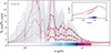 |
Fig. 8. Contribution of AGN emission to the PRIMAger bandpass. Thin grey lines show a z = 2 galaxy SED including different AGN properties (see Table 2), divided by the SED without an AGN component. As an example, the emission of one AGN model with different fAGN contributions (15, 30, and 45% of the total IR luminosity) is shown in red thick lines. The fluxes obtained for integration in the equivalent filters with centre wavelengths listed in Table 1 for PHI+PPI1+PPI2 are shown as red circles. The inset panel shows the SEDs corresponding to the red lines (for fAGN = 0% and fAGN = 45%) over the full UV to submm wavelength range. The PRIMAger bands are well suited to probing the impact of AGN emission on the IR SED of galaxies. |
We associate flux errors to the modelled fluxes, considering both the contribution from the instrumental (Table 1) and the confusion noise. We use the PHI1_4 filter (λ = 34 μm) as the detection band – because observations at that wavelength will not suffer from confusion (Béthermin et al. 2024) – and compute the fluxes in the remaining filters from their ratio to PHI1_4, while maintaining the overall SED shape. Classical confusion noise is usually derived for a blind detection strategy at a single wavelength, but PRIMAger’s broad and dense wavelength coverage enables more refined strategies that overcome such limitations. Donnellan et al. (2024) show that a self-contained Bayesian deblending approach implemented using XID+ (Hurley et al. 2017) reaches flux densities a factor of ∼2 − 3 fainter than the classical confusion limit estimated in Béthermin et al. (2024). We thus take the confusion noise values found by Donnellan et al. (2024) using their Wiener-filter derived catalogue, add them in quadrature to the instrumental noise to determine the total noise, and require a signal-to-noise ratio (S/N) of 10 in the PHI1_4 filter for our recovery experiment. We also compute the results requiring S/N = 5 in PHI1_4, which show a mild degradation and are in general intermediate between the extraction with PPI1+PPI2 and just PPI1 alone. We also show the result of a run using S/N = 10 and the lower confusion noise obtained in XID+ extractions when using a deep catalogue with some prior intensity information (Donnellan et al. 2024).
To test the quality of the parameter extraction, we fit the mock catalogue for qPAH, fAGN, and LIR simultaneously using the Bayesian-like analysis performed in CIGALE. We first do a run including data from PHI, then a run using PHI+PPI1, and then a final run using PHI+PPI1+PPI2. Figure 9 shows the distribution of the difference between the physical properties estimated through this process and their true value, considering galaxies with redshifts of 1 and 2. Broadly speaking, the histograms show very little or no bias for qPAH and fAGN, while there is a mild bias in LIR when the PPI filters are not included. As expected, the histograms also tighten up when more wavelength information is included, and they show little to no degradation if the S/N is dropped from 10 to 5 at our anchoring filter PHI_4.
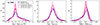 |
Fig. 9. Normalised distributions of the difference between the estimated and the true values of the extracted parameters. In each panel, the lines are colour coded according to the set of filters used in the fitting. The distributions include all models whose parameters are described in Table 2. The same distributions, with the PHI+PPI1+PPI2 set of filters but assuming a S/N of 5 instead of 10 in PHI1_4 are shown with a dashed line. The dotted line shows the results using the confusion noise for the deep catalogue from Donnellan et al. (2024), attainable in regions where ancillary information exists (e.g. from the Roman Space Telescope). Left panel: PAH fraction measured in percent (qPAH). Centre panel: AGN fractional contribution to the total IR luminosity (fAGN). Right panel: Total IR luminosity (log LIR). The distributions do not show any bias for the estimate of the PAH fraction and the AGN fraction at z = 1 and z = 2. The log LIR estimated with only the PHI presents a bias of +0.07 dex and a tail toward larger underestimates (factors of 2 to 3). Dropping the required S/N from 10 to 5 in the PHI1_4 has only a very modest impact on qPAH and fAGN and does not introduce any bias. |
Quantitatively, the histograms show a number of trends. Because the PAH emission is weakened or erased from the SED in the presence of a strong AGN continuum, we tested the recovery of qPAH in cases where there is no AGN contribution. The impact of reducing the wavelength coverage is on the width of the distribution, going from a dispersion of 0.9 with the full PHI plus two first filters of PPI to a flatter distribution when only using PHI (dispersion of 1.3). The AGN fractional contribution to the total LIR (fAGN) is well recovered when the full PHI band and the two first PPI filters are used: the distribution is centred on zero and has a dispersion of 0.06. The bias introduced by removing the PPI filters is very slight, just 0.02, and the dispersion increases by 30% to 0.08. Finally, the distribution of the difference between the estimated LIR and its true value, in logarithmic scale, is centred on zero and has a dispersion of 0.1 dex when all filters are included, but the median is biased high to +0.05 with a dispersion of 0.15 dex when we rely on PHI only.
It is also interesting to look at how the extraction results for fAGN and LIR vary as a function of both qPAH and fAGN. We show the systematic error and dispersion in our extraction in Fig. 10 computed for z = 1 and z = 2, when employing a filter set that includes the full PHI, and PPI1 + PPI2. The dispersion of the fAGN − fAGN, true distribution is on average 0.05, and below 0.12 over most of the parameter space. The highest uncertainty is found at z = 2 for very low intrinsic PAH abundance, qPAH < 2%, and intermediate AGN contributions, 0.15 < fAGN < 0.35. These tests show that the PRIMAger bands are well suited to probing the AGN emission and to disentangling it from the emission due to SF for a vast range of source properties. The bottom row of Fig. 10 shows that the LIR is very well recovered at z = 1 with a dispersion on the log LIR − log LIR, true distribution well below 0.12 dex for all the parameter space explored. At z = 2, the filters probe shorter rest-frame wavelengths, further away from the peak in the FIR, but the combined use of the PHI and the two first filters of PPI still allows for good recovery of the LIR with an average dispersion of 0.1 dex and a maximum of 0.25 dex.
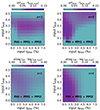 |
Fig. 10. Extraction of fAGN and LIR as a function of AGN contribution and PAH fraction. The AGN fraction is well recovered over the entire parameter range probed by the test, with an error of < 0.1 at both z = 1 and z = 2. The IR luminosity is recovered to better than 0.12 dex at z = 1, and with a dispersion of lower than < 0.25 dex at z = 2. Top row: Panels are colour coded according to the standard deviation of the fAGN − fAGN, true distribution. Left and right panels present the results at z = 1 and z = 2, respectively. Bottom row panels: Same as top row panels but for the LIR. |
To understand the impact of the longest wavelength SED points on the accuracy of the extracted parameters, we show in Fig. 11 the median value of the distributions shown in Figs. 9 and 10 for fAGN and LIR at z = 2, after removing one or both PPI filters. When removing the PPI2 filter (left column), fAGN is still well recovered with a bias that is lower than 0.05 in half of the parameter space tested here, except in the region of weak PAH and intermediate AGN contribution where it can reach up to 0.15, while for the LIR the bias can reach up to 0.25 dex. If only the full PHI band is used (right column), biases for fAGN and LIR also reach up to 0.15 and 0.25 dex, respectively, but over a wider proportion of the parameter space. Therefore, we conclude that the inclusion of the PPI fluxes is necessary to derive accurate PAH, SFR, and AGN parameters, particularly for sources at z = 2 where the PHI band probes only up to 27 μm rest-frame wavelengths.
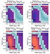 |
Fig. 11. Impact of removing long wavelength information at z = 2 on parameter extraction accuracy. Top row: Median value of fAGN − fAGN, true as a function of fAGN and LIR. Bottom row: Same but for log LIR − log LIR, true. The left side and right side panels show values where the PHI band plus PPI1 band and those only in the full PHI band are used to extract the parameters, respectively. |
3.2.2. Expected distributions
State-of-the-art galaxy evolution models show order-of-magnitude disagreements in their predictions of the distribution of the ratio of BHAR/SFR (Habouzit et al. 2020, 2021). In general, models calibrated on physical quantities derived from UV, optical, and near-infrared (NIR) data (e.g. stellar mass, SFR), such as IllustrisTNG and the SC SAM (Somerville et al. 2008, 2015), predict faster black hole growth at higher masses and luminosities, with the consequent quenching of SF activity. Empirical models calibrated on FIR data from the Herschel telescope, such as SPRITZ and Simulated Infrared Dusty Extragalactic Sky (SIDES, Béthermin et al. 2017), on the other hand, predict slower black-hole growth and more vigorous dust-enshrouded SF in luminous systems. The main reason for this discrepancy is that much of the stellar and black hole growth takes place behind large screens of gas and dust that absorbs photons from the NIR to the soft X-ray bands (Hickox & Alexander 2018).
Figure 12 shows a comparison of the z = 1 − 1.5 slice of a survey of a galaxy population synthesised using SPRITZ with the same slice synthesised using the SC SAM over the same 10 sq. deg. light cone (Yung et al. 2022). These calculations use the depth attainable with the conservative performance of PRIMAger in 150 hours per square degree (i.e. Wide survey in Table 1) and the extraction depth attainable using a source extraction based on the software XID+ (Donnellan et al. 2024), which requires that the sources are detected at 5σ or better over half the bandpass of PHI. The key difference is that SPRITZ predicts a much larger number of composite AGN-starburst systems, as well as many more galaxies with larger SFRs than the SC SAM. In the SC SAM, only ∼4% of the galaxies have BHAR > 0.06 M⊙ yr−1 and SFR > 20 M⊙ yr−1, while for SPRITZ that fraction is ∼44%. The fairly large discrepancy between models highlights the urgent need for deep surveys with a sensitive FIR telescope like PRIMA that can disentangle SF and AGN powered emission within large numbers of dusty galaxies at cosmic noon. The fast mapping capabilities of PRIMA will enable sample sizes detected with PRIMAger that are between 100 and 1000 times larger than those available from Herschel (Magnelli et al. 2013; Delvecchio et al. 2014), providing us with a true statistical view of black hole and SF activity during the formative era of galaxies.
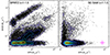 |
Fig. 12. Comparison of expected galaxy distributions in SFR and BHAR from SPRITZ and the Santa Cruz SAM over a 10 sq. deg light cone with an integration time of ∼150 h per square degree. The contours indicate the density of sources, and the magenta cross in the right panel shows the expected extraction uncertainties for the median galaxy (Sect. 2.4). Each panel has about 30 000 sources detected at 5σ or better over half the PHI bandpass, but only ∼4% are hybrid AGN+SF galaxies in the SC SAM, while ∼44% of the SPRITZ sources are hybrid. In models like the SC SAM, the rapid growth of the black hole leads to stopping the SF activity, while empirical models calibrated against FIR data, such as SPRITZ, predict a large number of co-evolving systems. |
3.3. SFR versus BHAR with FIRESS using FIR lines
As mentioned above, FIR spectroscopy can be used to obtain a direct estimate of both the BHAR and the SFR for the same object. Indeed, the [O IV]26 μm line is a robust calibration of the BHAR, while the [Ne II]13 μm line is an accurate indicator of the SFR (e.g. Spinoglio et al. 2015; Stone et al. 2022). In the case of the [O IV]26 μm line, the contribution excited by SF can be accounted for (Stone et al. 2022), and the blended contribution from the much fainter nearby [Fe II]26 μm line will not affect the measurement. Figure 13 shows how the predicted flux of these two lines changes with IR luminosity, AGN fraction (defined between 8 and 1000 μm), and redshift, as derived from SPRITZ.
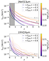 |
Fig. 13. Evolution of line fluxes with redshift, IR luminosity and AGN fraction. Spectroscopic follow-up analyses of galaxies down to 10−19 W/m2 will start probing more normal galaxies and not only ultraluminous IR galaxies. We show the [Ne II]13 μm (top) and [O IV]26 μm (bottom) line fluxes as a function of redshift, total IR luminosity (see colour bar), and IR-AGN fraction (different line styles in bins with ΔfAGN = 0.2). Dashed dotted lines indicate the line fluxes for galaxies in the knee of the IR luminosity function and six times above it (Traina et al. 2024). The grey area in the top panel shows the redshift range in which the [Ne II]13 μm line is not in the PRIMA/FIRESS wavelength coverage. |
We concentrate on fluxes down to 10−19 W/m2, which is feasible for point sources with FIRESS in the low-resolution mode (R ∼ 100) with one hour of integration time. However, we highlight that this depth is simply chosen as an example and that it is indeed possible to integrate more time with FIRESS. More specifically, observations down to 10−19 W/m2 allow the [Ne II]13 μm line to be traced in galaxies of LIR = 1011 L⊙ up to z = 0.7, while galaxies of LIR = 1012.5 L⊙ can be observed up to z = 3. These fluxes show little dependence on the AGN fraction, given that the [Ne II]13 μm line mainly traces SF. The [O IV]26 μm line, which efficiently traces AGN activity, is instead generally fainter than the [Ne II]13 μm line, and therefore similar observations trace galaxies of LIR = 1011.0 L⊙ up to z = 0.4 for fAGN < 0.5, but up to z = 0.8 for higher AGN fractions. At the same time, the [O IV]26 μm line is brighter than 10−19 W/m2 in galaxies of LIR = 1012.5 L⊙ up to z = 1, if fAGN < 0.5, and up to z = 1.8 for higher AGN fractions. To put these values in a broader context, we also report the line fluxes for galaxies at the knee of the IR luminosity function, as derived by Traina et al. (2024), and six times above it. The galaxies with a [O IV]26 μm or [Ne II]13 μm line brighter than 10−19 W/m2 are generally beyond the knee of the luminosity function, but are not tracing hyperluminous IR galaxies (LIR > 1013 L⊙). Moreover, it is necessary to take into account that there will be several other low-ionisation FIR fine-structure lines that trace SF or AGN. Correlating these lines could potentially enable us to detect galaxies to greater depth and bolster our confidence in the weaker line detections.
In order to simultaneously derive SFR and BHAR to trace possible signatures of co-evolution between the AGN and its host galaxy, it is necessary to observe both [O IV]26 μm and [Ne II]13 μm in the same galaxies. This will be possible only for a subsample of the aforementioned objects, whose redshift distribution is shown in Fig. 14. This subsample corresponds to around 19 000 objects/deg2 up to z = 5.5, of which ∼15 800 objects/deg2 are at z > 0.8 and inside the FIRESS wavelength coverage. Among the latter, 91% and 59% of the galaxies are expected to also be detected with PRIMAger above the Deep and Wide depths, respectively. In particular, the deep photometric survey includes > 90% and > 50% of objects with [O IV]26 μm and [Ne II]13 μm up to z = 2 and z = 3.6. Therefore, the Deep PRIMAger photometric survey can efficiently be used to select targets to follow up in spectroscopy in order to validate and calibrate the SFR and BHAR derived through the SED-fitting analysis.
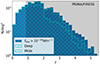 |
Fig. 14. Redshift distribution of line-detected galaxies. The photometric survey can be used to identify galaxies to follow-up in spectroscopy. We show the redshift distribution of galaxies with [O IV]26 μm and [Ne II]13 μm lines above 10−19 W/m2 (blue histogram) with the subsamples detected in the Deep and Wide surveys (hatched histograms), considering the conservative depths. The grey area shows the redshift range in which [O IV]26 μm and [Ne II]13 μm lines are in the PRIMA/FIRESS wavelength coverage, but other lines can be used at z < 0.8 to derive SFR and BHAR. |
3.4. PAH metallicity dependence
Up to 20% of the total IR emission in galaxies emerges as vibrational emission at 3−18 μm of small carbon-rich PAH grains (Smith et al. 2007). Spitzer observations of PAHs in the local Universe uncovered a strong dependency of the strength of PAH emission on the gas-phase metallicity, with an apparent steep decline in the PAH abundance at metallicities of less than ∼25% solar (Engelbracht et al. 2005; Smith et al. 2007; Draine et al. 2007; Hunter et al. 2010; Sandstrom et al. 2012; Aniano et al. 2020; Whitcomb et al. 2023). This connection between small grain emission and gas metal abundance ties directly to the lifecycle of PAHs, with indications from changing-size and heating-sensitive band ratios of strong evolution in the distribution of grain sizes and potential photo-destruction in high intensity, UV-bright radiation environments. As explored by Calzetti et al. (2007), the metallicity dependence of PAH emission also impacts their use and calibration as indicators of SFR and AGN fraction.
JWST is now uncovering evidence that PAHs are deficient in lower mass (and likely lower metallicity) galaxies approaching cosmic noon (Shivaei et al. 2024), and has also identified unexpectedly strong UV absorption in the 2100 Å feature sometimes attributed to PAHs at redshifts as high as z = 7 (Witstok et al. 2023). JWST spectroscopic mapping observation of a strongly lensed dusty luminous galaxy at z = 4.1 revealed strongly varying PAH 3.3 μm emission (Spilker et al. 2023), in what is currently the earliest known PAH detection. Nevertheless, the majority of PAH power shifts out of JWST’s passbands by z = 2.1, and the long-wavelength spectroscopic sensitivity of the JWST Mid-Infrared Instrument limits the study of PAH emission to the single 3.3 μm band, which comprises just a few percent of the total PAH luminosity (Lai et al. 2020). At cosmic noon and earlier times, the bulk of PAH power shifts into PRIMA’s FIR passbands (see Fig. 1).
SPRITZ predicts that samples of the order of ∼104 PAH-emitting galaxies will be detected in the deep hyper-spectral survey (Fig. 6), including luminous sources out to z = 8. At z ∼ 2, the metallicity measure based on [N III]57 μm, [O III]52 μm, and [O III]88 μm lines (N3O3 method, Sect. 2.2.1) can be combined with direct hyper-spectral and spectroscopic recovery of PAH luminosity to directly test models of PAH lifecycle and metal sensitivity during the epoch when dust and metal production peaked in the Universe. As visible in Fig. 15, we expect 850 objects/deg2 to have all three lines necessary for the measurement of N3O3 (i.e. [N III]57 μm, [O III]52 μm, and [O III]88 μm) above 10−19 W/m2 at z < 1.7, which is the maximum redshift at which FIRESS can observe [O III]88 μm. Almost all (> 98%) of these galaxies are expected to be detected in the PRIMAger surveys. At z = 1.5 − 2.5, we instead expect to observe around 2000 objects/deg2 with both [N III]57 μm and [O III]52 μm lines above the same flux limit. Moreover, considering the conservative depths, 72% and 43% of these objects will be detected in the PRIMAger Deep and Wide surveys, respectively. These fractions change by 1% or less if we consider the payload sensitivities. This shows that the Deep photometric survey can be used to select objects prior to follow up with FIRESS.
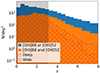 |
Fig. 15. Redshift distribution predicted in SPRITZ for galaxies with [N III]57 μm, [O III]52 μm, and/or [O III]88 μm lines above 10−19 W/m2. The hatched histogram shows the subpopulation that is also detected in the Deep and Wide PRIMAger surveys, considering the conservative depths. The grey area shows the redshift range in which [N III]57 μm and [O III]52 μm lines are in the PRIMA/FIRESS wavelength coverage. |
3.5. Predicting and observing galactic outflows
Galactic outflows, whether driven by AGN or the collective effects of supernovae, are believed to play an important role in galaxy evolution. These outflows can heat or even entirely remove the gas available for future SF, and can reduce or halt gas infall from the CGM. Outflows are known to be very common in luminous and ultraluminous IR galaxies in the local Universe (e.g. Veilleux et al. 2013), with velocities that can exceed 1000 km s−1. They are invariably multi-phase, with a cool component that is thought to dominate the mass and momentum of the outflow. This cool component can be observed and characterised directly in the FIR, most commonly via FIR OH lines observed in absorption against the FIR continuum of the host galaxy (Spoon et al. 2013; Veilleux et al. 2013; Stone et al. 2016). In particular, mass-outflow rates can be derived using OH rotational doublets at 65, 71, 79, and 84 μm and used in conjunction with radiative-transfer models to estimate the physical parameters of the cool component of the wind, most importantly the mass and mass-outflow rates, which can match and in some cases exceed the SFRs even in the most luminous galaxies (González-Alfonso et al. 2017).
We rely on simulations to predict the occurrence of outflows and estimate their properties over cosmic time. Hydrodynamical simulations, in particular, can be used to model the properties and effects of outflows in individual and ensembles of galaxies, but the detailed physics and implementation varies significantly (Wright et al. 2024). Just as importantly, these simulations are extremely costly to run, and it is unfeasible to simulate the large volumes that will be surveyed by future telescopes like PRIMA. All simulations predict strong outflows associated with rapidly growing galaxies and SMBHs, although the details vary from one simulation to the next. To estimate the galactic outflows that we can expect to study with PRIMA, we use scaling relations extracted from one such simulation and ‘paint’ them on top of the galaxy population in the SPRITZ model. In order to do this, we make use of the galactic outflows in IllustrisTNG Wright et al. (2024), and statistically relate them to galaxy properties as available in both IllustrisTNG and SPRITZ. We start by converting the BHARs and SFRs to galaxy bolometric luminosities using the standard recipes (assuming an efficiency of 10% for the accretion, and using the Kennicutt & Evans 2012, conversion between SFR and luminosity). We then derive a relation between bolometric luminosity and outflow mass-loss rate (Ṁout), as measured at a scale of 0.1 rvir from the centre of the galaxy halo at redshift z = 2, where rvir is the halo virial radius.
These results in a correlation between the mass-outflow rate (in M⊙ yr−1) and the bolometric luminosity (in L⊙), such that log(Ṁout) = 0.54 log(Lbol) − 4.13, with a tail of objects that scatter toward higher mass-loss rates (Figure 16). The relative importance of the tail is greater when considering systems with higher outflow velocities, containing just over 2% of the systems with outflows at 0.1 rvir to just over 7% for systems with outflow velocities of ≥250 km s−1 at 0.1 rvir. We note that a system being in the high-velocity tail of the distribution does not correlate with it harbouring an energetically important AGN at the time of the measurement (red symbols in Figure 16), and may instead reflect past AGN activity.
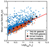 |
Fig. 16. Correlation between bolometric luminosity and outflow mass-loss rate in IllustrisTNG simulations. Red square symbols represent galaxies where the AGN has ≥20% contribution to Lbol, while blue symbols are all other galaxies. The median mass-loss rate in bins of Lbol is shown by the black symbols. The main correlation, log(Ṁoutf) = 0.54 log(Lbol) − 4.13, is shown by the red line. |
Figure 17 shows the result of applying the relation described above to the SPRITZ simulations of the IR sky. Since the models are sparsely populated at the high-luminosity end, an assumption here is that the derived relation can be extrapolated to galaxies with very large bolometric luminosities (approaching or even exceeding 1013 L⊙). This is reasonable because these luminous systems represent dusty galaxies where the stellar mass and/or the central black hole are accreting and growing at their largest rates, and these are also expected to host the most powerful outflows – just as they do at low redshift when they are much more rare. Figure 17 shows the density of systems that would be well detected (those detected at 5σ or larger over more than 50% of the PRIMAger Hyper-spectral Imager logarithmic passband) in a PRIMAger survey with 150 hours of integration per square degree, at the conservative performance expected for the instrument. By scaling results obtained for the outflow in the nearby ultraluminous IR galaxy Mrk 231 (González-Alfonso et al. 2014), we estimate that it is possible to use FIRESS operating at R ≈ 900 to detect and characterise these winds via the 84 μm OH line for over 200 luminous IR galaxies detected with PRIMAger at z ∼ 1 − 2 (those brighter than 120 mJy at 210 μm). This will expand the number of sources with powerful, massive outflows studied spectroscopically in the FIR by more than an order of magnitude, and will allow us to probe quenching in dusty galaxies at cosmic noon –and the subsequent decline in SF– for the first time.
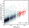 |
Fig. 17. Predicted mass-loss rates. We show galaxies in SPRITZ well detected with PRIMAger in a 10 sq. deg. survey with 150 hours of integration per square degree for the redshift range 1.5 < z < 2, using an extrapolation of the relation described in Sect. 3.5. The red galaxies (about 200 of them) are brighter than 120 mJy at 210 μm, and thus can be followed up in velocity-resolved OH absorption spectroscopy in a moderate integration. These are very rapidly growing systems expected to host massive winds. |
4. Summary and conclusions
The most active phases of SF and black hole accretion in galaxies are hidden behind large columns of gas and dust. Studying critical phases in the co-evolution of SMBHs and galaxies therefore requires the ability to penetrate the resulting extinction, and bring to bear sensitive diagnostic tools to study the physical conditions in distant galaxies. The MIR and FIR part of the spectrum provides abundant well-understood diagnostics of the atomic and molecular gas, as well as the dust, providing a window onto SF, black hole growth, metallicity, and feedback-driven galactic outflows in even the most obscured galaxies. In this work, we demonstrate the photometric and spectroscopic capabilities of the PRIMA mission to address key questions regarding our understanding of how galaxies and SMBHs evolve together over a significant fraction of cosmic time.
In particular, we show that multi-tiered photometric surveys conducted with PRIMAger will allow us to detect and study galaxies hundreds of times fainter than were reachable by previous FIR observatories (e.g. Herschel, Spitzer), reaching the bulk of the population to cosmic noon and beyond. PRIMAger will be able to observe normal (1011 L⊙) star-forming galaxies up to z = 4, and its dense wavelength coverage efficiently probes the presence of PAHs for z ≳ 1 and can also be used to accurately separate AGN and SF heating by measuring the shape of the IR dust continuum. Using simulations based on the deepest existing FIR surveys, along with semi-analytic models of evolving galaxies and dark matter halos, we make predictions of the galaxy populations that could be observed with PRIMAger and FIRESS, along with quantitative estimates of the accuracies with which we can disentangle and measure the signatures of SF, black hole growth, gas-phase metallicity, and galactic outflows as a function of IR luminosity, redshift, and survey area. In particular, we verified that, using SED-decomposition, we are able to retrieve the AGN fraction with respect to the total IR luminosity with a dispersion of 0.06, the fraction of dust mass contributed by PAH (qPAH, measured in percentage) with a dispersion of 0.9, and the total IR luminosity with a scatter of 0.1 dex (Sect. 2.4). Because of its ability to map large areas of the sky to great depths, PRIMA can be used to generate and measure large samples of dusty galaxies that are between 100 and 1000 times larger than those available from Herschel (Magnelli et al. 2013; Delvecchio et al. 2014) out to the epoch of peak SF and black hole growth.
Spectroscopic follow up with the FIRESS instrument on PRIMA will reach unprecedented depths in the FIR –that is, 10−19 W/m2 in one hour of integration at R = 100– allowing detection of faint fine-structure lines and PAH emission features, which can be used to directly estimate SF and black hole accretion rates in distant galaxies. Using FIRESS, it will be possible to measure the [O IV]26 μm and [Ne II]13 μm fine-structure lines, and hence the BHAR and SFR in galaxies of 1012.5 L⊙ up to z ∼ 1.8 and z ∼ 3, respectively. We expect around 16 000 object/deg2 with both [O IV]26 μm and [Ne II]13 μm lines brighter than 10−19 W/m2 at z > 0.8, with the large majority (> 90%) of them securely detected in at least half of the 12 PRIMAger bands. At the same spectroscopic depths, we expect over 2000 object/deg2 at z = 1.5 − 2.5, which could be followed up with FIRESS to derive metallicity measurements using the [N III]57 μm and [O III]52 μm emission lines. When combined with measures of the PAH emission features, which are easily detectable with FIRESS at z > 2, it will be possible to study the connection between small-grain emission and gas metal abundance in thousands of distant galaxies.
Finally, we used the models and correlations between bolometric luminosity and outflow mass and velocity seen in the local Universe to predict that, with a modest amount of observing time, it will be possible to detect and characterise the galactic outflows with the high-resolution mode of FIRESS using the OH molecular absorption feature in more than 200 galaxies to z ∼ 1 − 2. These observations will expand the number of galactic outflows measured in the FIR by nearly an order of magnitude, and will allow us to test whether such outflows are sufficient to quench SF in bright IR galaxies over the past 10 Gyr of cosmic time.
Acknowledgments
The authors acknowledge the scientific help of John Arballo and the PRIMA extragalactic science working groups. LB acknowledges support from INAF under the Large Grant 2022 funding scheme (project “MeerKAT and LOFAR Team up: a Unique Radio Window on Galaxy/AGN co-Evolution”). LC acknowledges support from the french government under the France 2030 investment plan, as part of the Initiative d’Excellence d’Aix-Marseille Université – A*MIDEX AMX-22-RE-AB-101. RJW acknowledges support from the European Research Council via ERC Consolidator Grant KETJU (no. 818930).
References
- Akiyama, M., He, W., Ikeda, H., et al. 2018, PASJ, 70, S34 [NASA ADS] [CrossRef] [Google Scholar]
- Aniano, G., Draine, B. T., Hunt, L. K., et al. 2020, ApJ, 889, 150 [NASA ADS] [CrossRef] [Google Scholar]
- Armus, L., Charmandaris, V., Spoon, H. W. W., et al. 2004, ApJS, 154, 178 [NASA ADS] [CrossRef] [Google Scholar]
- Armus, L., Bernard-Salas, J., Spoon, H. W. W., et al. 2006, ApJ, 640, 204 [NASA ADS] [CrossRef] [Google Scholar]
- Armus, L., Charmandaris, V., Bernard-Salas, J., et al. 2007, ApJ, 656, 148 [NASA ADS] [CrossRef] [Google Scholar]
- Armus, L., Lai, T., U, V., et al. 2023, ApJ, 942, L37 [NASA ADS] [CrossRef] [Google Scholar]
- Arnouts, S., Walcher, C. J., Le Fèvre, O., et al. 2007, A&A, 476, 137 [CrossRef] [EDP Sciences] [Google Scholar]
- Baselmans, J. 2012, J. Low Temp. Phys., 167, 292 [CrossRef] [Google Scholar]
- Beare, R., Brown, M. J. I., Pimbblet, K., & Taylor, E. N. 2019, ApJ, 873, 78 [NASA ADS] [CrossRef] [Google Scholar]
- Bernard Salas, J., Pottasch, S. R., Beintema, D. A., & Wesselius, P. R. 2001, A&A, 367, 949 [NASA ADS] [CrossRef] [EDP Sciences] [Google Scholar]
- Berta, S., Lutz, D., Santini, P., et al. 2013, A&A, 551, A100 [NASA ADS] [CrossRef] [EDP Sciences] [Google Scholar]
- Béthermin, M., Wu, H.-Y., Lagache, G., et al. 2017, A&A, 607, A89 [Google Scholar]
- Béthermin, M., Bolatto, A. D., Boulanger, F., et al. 2024, ArXiv e-prints [arXiv:2404.04320] [Google Scholar]
- Bianchi, S., De Vis, P., Viaene, S., et al. 2018, A&A, 620, A112 [NASA ADS] [CrossRef] [EDP Sciences] [Google Scholar]
- Bisigello, L., Gruppioni, C., Feltre, A., et al. 2021, A&A, 651, A52 [NASA ADS] [CrossRef] [EDP Sciences] [Google Scholar]
- Bisigello, L., Vallini, L., Gruppioni, C., et al. 2022, A&A, 666, A193 [NASA ADS] [CrossRef] [EDP Sciences] [Google Scholar]
- Bisigello, L., Gandolfi, G., Grazian, A., et al. 2023, A&A, 676, A76 [NASA ADS] [CrossRef] [EDP Sciences] [Google Scholar]
- Bonato, M., De Zotti, G., Leisawitz, D., et al. 2019, PASA, 36, e017 [NASA ADS] [CrossRef] [Google Scholar]
- Boquien, M., Burgarella, D., Roehlly, Y., et al. 2019, A&A, 622, A103 [NASA ADS] [CrossRef] [EDP Sciences] [Google Scholar]
- Brightman, M., & Nandra, K. 2011, MNRAS, 413, 1206 [NASA ADS] [CrossRef] [Google Scholar]
- Calzetti, D., Kennicutt, R. C., Engelbracht, C. W., et al. 2007, ApJ, 666, 870 [Google Scholar]
- Chabrier, G. 2003, PASP, 115, 763 [Google Scholar]
- Chartab, N., Cooray, A., Ma, J., et al. 2022, Nat. Astron., 6, 844 [NASA ADS] [CrossRef] [Google Scholar]
- Ciesla, L., Boquien, M., Boselli, A., et al. 2014, A&A, 565, A128 [NASA ADS] [CrossRef] [EDP Sciences] [Google Scholar]
- Ciesla, L., Charmandaris, V., Georgakakis, A., et al. 2015, A&A, 576, A10 [NASA ADS] [CrossRef] [EDP Sciences] [Google Scholar]
- Cirasuolo, M., McLure, R. J., Dunlop, J. S., et al. 2007, MNRAS, 380, 585 [NASA ADS] [CrossRef] [Google Scholar]
- Croom, S. M., Richards, G. T., Shanks, T., et al. 2009, MNRAS, 399, 1755 [NASA ADS] [CrossRef] [Google Scholar]
- da Cunha, E., Charlot, S., & Elbaz, D. 2008, MNRAS, 388, 1595 [Google Scholar]
- Dale, D. A., Smith, J. D. T., Armus, L., et al. 2006, ApJ, 646, 161 [NASA ADS] [CrossRef] [Google Scholar]
- Day, P. K., LeDuc, H. G., Mazin, B. A., Vayonakis, A., & Zmuidzinas, J. 2003, Nature, 425, 817 [NASA ADS] [CrossRef] [Google Scholar]
- Day, P. K., Cothard, N. F., Albert, C., et al. 2024, ArXiv e-prints [arXiv:2404.10246] [Google Scholar]
- De Looze, I., Cormier, D., Lebouteiller, V., et al. 2014, A&A, 568, A62 [NASA ADS] [CrossRef] [EDP Sciences] [Google Scholar]
- Delvecchio, I., Gruppioni, C., Pozzi, F., et al. 2014, MNRAS, 439, 2736 [NASA ADS] [CrossRef] [Google Scholar]
- Díaz-Santos, T., Armus, L., Charmandaris, V., et al. 2013, ApJ, 774, 68 [Google Scholar]
- Donnellan, J. M. S., Oliver, S. J., Bethermin, M., et al. 2024, MNRAS, 532, 1966 [NASA ADS] [CrossRef] [Google Scholar]
- Draine, B. T. 2003, ARA&A, 41, 241 [NASA ADS] [CrossRef] [Google Scholar]
- Draine, B. T. 2011, Physics of the Interstellar and Intergalactic Medium (Princeton: Princeton University Press) [Google Scholar]
- Draine, B. T., Dale, D. A., Bendo, G., et al. 2007, ApJ, 663, 866 [NASA ADS] [CrossRef] [Google Scholar]
- Draine, B. T., Aniano, G., Krause, O., et al. 2014, ApJ, 780, 172 [Google Scholar]
- Dwek, E., & Cherchneff, I. 2011, ApJ, 727, 63 [NASA ADS] [CrossRef] [Google Scholar]
- Engelbracht, C. W., Gordon, K. D., Rieke, G. H., et al. 2005, ApJ, 628, L29 [NASA ADS] [CrossRef] [Google Scholar]
- Euclid Collaboration (Bisigello, L., et al.) 2024, A&A, submitted [Google Scholar]
- Feltre, A., Charlot, S., & Gutkin, J. 2016, MNRAS, 456, 3354 [Google Scholar]
- Feltre, A., Gruppioni, C., Marchetti, L., et al. 2023, A&A, 675, A74 [NASA ADS] [CrossRef] [EDP Sciences] [Google Scholar]
- Ferland, G. J., Porter, R. L., van Hoof, P. A. M., et al. 2013, Rev. Mex. Astron. Astrofis., 49, 137 [Google Scholar]
- Fernández-Ontiveros, J. A., Spinoglio, L., Pereira-Santaella, M., et al. 2016, ApJS, 226, 19 [CrossRef] [Google Scholar]
- Fernández-Ontiveros, J. A., Armus, L., Baes, M., et al. 2017, PASA, 34, e053 [CrossRef] [Google Scholar]
- Ferrarese, L. 2002, ApJ, 578, 90 [NASA ADS] [CrossRef] [Google Scholar]
- González-Alfonso, E., Fischer, J., Graciá-Carpio, J., et al. 2014, A&A, 561, A27 [NASA ADS] [CrossRef] [EDP Sciences] [Google Scholar]
- González-Alfonso, E., Fischer, J., Spoon, H. W. W., et al. 2017, ApJ, 836, 11 [Google Scholar]
- Greene, J. E., Labbe, I., Goulding, A. D., et al. 2024, ApJ, 964, 39 [CrossRef] [Google Scholar]
- Gruppioni, C., Pozzi, F., Andreani, P., et al. 2010, A&A, 518, L27 [NASA ADS] [CrossRef] [EDP Sciences] [Google Scholar]
- Gruppioni, C., Pozzi, F., Rodighiero, G., et al. 2013, MNRAS, 432, 23 [Google Scholar]
- Gruppioni, C., Calura, F., Pozzi, F., et al. 2015, MNRAS, 451, 3419 [Google Scholar]
- Gruppioni, C., Berta, S., Spinoglio, L., et al. 2016, MNRAS, 458, 4297 [Google Scholar]
- Gruppioni, C., Béthermin, M., Loiacono, F., et al. 2020, A&A, 643, A8 [NASA ADS] [CrossRef] [EDP Sciences] [Google Scholar]
- Gültekin, K., Cackett, E. M., Miller, J. M., et al. 2009, ApJ, 706, 404 [CrossRef] [Google Scholar]
- Habouzit, M., Pisani, A., Goulding, A., et al. 2020, MNRAS, 493, 899 [NASA ADS] [CrossRef] [Google Scholar]
- Habouzit, M., Li, Y., Somerville, R. S., et al. 2021, MNRAS, 503, 1940 [NASA ADS] [CrossRef] [Google Scholar]
- Harikane, Y., Zhang, Y., Nakajima, K., et al. 2023, ApJ, 959, 39 [NASA ADS] [CrossRef] [Google Scholar]
- Herrera-Camus, R., Bolatto, A., Smith, J. D., et al. 2016, ApJ, 826, 175 [Google Scholar]
- Hickox, R. C., & Alexander, D. M. 2018, ARA&A, 56, 625 [Google Scholar]
- Hirschmann, M., Somerville, R. S., Naab, T., & Burkert, A. 2012, MNRAS, 426, 237 [NASA ADS] [CrossRef] [Google Scholar]
- Hopkins, P. F., Richards, G. T., & Hernquist, L. 2007, ApJ, 654, 731 [Google Scholar]
- Huertas-Company, M., Bernardi, M., Pérez-González, P. G., et al. 2016, MNRAS, 462, 4495 [CrossRef] [Google Scholar]
- Hunter, D. A., Elmegreen, B. G., & Ludka, B. C. 2010, AJ, 139, 447 [NASA ADS] [CrossRef] [Google Scholar]
- Hurley, P. D., Oliver, S., Betancourt, M., et al. 2017, MNRAS, 464, 885 [Google Scholar]
- Inami, H., Armus, L., Charmandaris, V., et al. 2013, ApJ, 777, 156 [Google Scholar]
- Kennicutt, R. C., & Evans, N. J. 2012, ARA&A, 50, 531 [NASA ADS] [CrossRef] [Google Scholar]
- Killi, M., Watson, D., Brammer, G., et al. 2023, ArXiv e-prints [arXiv:2312.03065] [Google Scholar]
- Kirkpatrick, A., Pope, A., Sajina, A., et al. 2015, ApJ, 814, 9 [NASA ADS] [CrossRef] [Google Scholar]
- Klypin, A., Yepes, G., Gottlöber, S., Prada, F., & Heß, S. 2016, MNRAS, 457, 4340 [Google Scholar]
- Kocevski, D. D., Onoue, M., Inayoshi, K., et al. 2023, ApJ, 954, L4 [NASA ADS] [CrossRef] [Google Scholar]
- Kocevski, D. D., Finkelstein, S. L., Barro, G., et al. 2024, ApJ, submitted [arXiv:2404.03576] [Google Scholar]
- Kormendy, J., & Ho, L. C. 2013, ARA&A, 51, 511 [Google Scholar]
- La Caria, M. M., Vignali, C., Lanzuisi, G., Gruppioni, C., & Pozzi, F. 2019, MNRAS, 487, 1662 [CrossRef] [Google Scholar]
- Lai, T. S. Y., Smith, J. D. T., Baba, S., Spoon, H. W. W., & Imanishi, M. 2020, ApJ, 905, 55 [NASA ADS] [CrossRef] [Google Scholar]
- Lai, T. S. Y., Armus, L., U, V., et al. 2022, ApJ, 941, L36 [NASA ADS] [CrossRef] [Google Scholar]
- Lamarche, C., Smith, J. D., Kreckel, K., et al. 2022, ApJ, 925, 194 [NASA ADS] [CrossRef] [Google Scholar]
- Lanzuisi, G., Perna, M., Delvecchio, I., et al. 2015, A&A, 578, A120 [NASA ADS] [CrossRef] [EDP Sciences] [Google Scholar]
- Larson, R. L., Finkelstein, S. L., Kocevski, D. D., et al. 2023, ApJ, 953, L29 [NASA ADS] [CrossRef] [Google Scholar]
- Madau, P., & Dickinson, M. 2014, ARA&A, 52, 415 [Google Scholar]
- Magnelli, B., Popesso, P., Berta, S., et al. 2013, A&A, 553, A132 [NASA ADS] [CrossRef] [EDP Sciences] [Google Scholar]
- Magorrian, J., Tremaine, S., Richstone, D., et al. 1998, ApJ, 115, 2285 [CrossRef] [Google Scholar]
- Maiolino, R., Scholtz, J., Curtis-Lake, E., et al. 2023, ArXiv e-prints [arXiv:2308.01230] [Google Scholar]
- Maiolino, R., Risaliti, G., Signorini, M., et al. 2024, ArXiv e-prints [arXiv:2405.00504] [Google Scholar]
- Małek, K., Buat, V., Roehlly, Y., et al. 2018, A&A, 620, A50 [Google Scholar]
- Matthee, J., Naidu, R. P., Brammer, G., et al. 2024, ApJ, 963, 129 [NASA ADS] [CrossRef] [Google Scholar]
- McConnell, N. J., Ma, C.-P., Gebhardt, K., et al. 2011, Nature, 480, 215 [NASA ADS] [CrossRef] [Google Scholar]
- McGreer, I. D., Jiang, L., Fan, X., et al. 2013, ApJ, 768, 105 [NASA ADS] [CrossRef] [Google Scholar]
- Mignoli, M., Feltre, A., Bongiorno, A., et al. 2019, A&A, 626, A9 [NASA ADS] [CrossRef] [EDP Sciences] [Google Scholar]
- Moffett, A. J., Ingarfield, S. A., Driver, S. P., et al. 2016, MNRAS, 457, 1308 [NASA ADS] [CrossRef] [Google Scholar]
- Moullet, A., Kataria, T., Lis, D., et al. 2023, ArXiv e-prints [arXiv:2310.20572] [Google Scholar]
- Mullaney, J. R., Daddi, E., Béthermin, M., et al. 2012, ApJ, 753, L30 [Google Scholar]
- Nagao, T., Maiolino, R., Marconi, A., & Matsuhara, H. 2011, A&A, 526, A149 [NASA ADS] [CrossRef] [EDP Sciences] [Google Scholar]
- Onoue, M., Inayoshi, K., Ding, X., et al. 2023, ApJ, 942, L17 [NASA ADS] [CrossRef] [Google Scholar]
- Peimbert, A., & Peimbert, M. 2010, ApJ, 724, 791 [NASA ADS] [CrossRef] [Google Scholar]
- Peng, B., Lamarche, C., Stacey, G. J., et al. 2021, ApJ, 908, 166 [NASA ADS] [CrossRef] [Google Scholar]
- Pereira-Santaella, M., Rigopoulou, D., Farrah, D., Lebouteiller, V., & Li, J. 2017, MNRAS, 470, 1218 [NASA ADS] [CrossRef] [Google Scholar]
- Pérez-González, P. G., Barro, G., Annunziatella, M., et al. 2023, ApJ, 946, L16 [CrossRef] [Google Scholar]
- Pérez-González, P. G., Barro, G., Rieke, G. H., et al. 2024, ApJ, 968, 4 [CrossRef] [Google Scholar]
- Pilyugin, L. S., Grebel, E. K., & Kniazev, A. Y. 2014, AJ, 147, 131 [NASA ADS] [CrossRef] [Google Scholar]
- Polletta, M., Tajer, M., Maraschi, L., et al. 2007, ApJ, 663, 81 [NASA ADS] [CrossRef] [Google Scholar]
- Reines, A. E., & Volonteri, M. 2015, ApJ, 813, 82 [NASA ADS] [CrossRef] [Google Scholar]
- Rieke, G. H., Alonso-Herrero, A., Weiner, B. J., et al. 2009, ApJ, 692, 556 [NASA ADS] [CrossRef] [Google Scholar]
- Rigby, J. R., Diamond-Stanic, A. M., & Aniano, G. 2009, ApJ, 700, 1878 [Google Scholar]
- Rodighiero, G., Bisigello, L., Iani, E., et al. 2023, MNRAS, 518, L19 [Google Scholar]
- Ross, N. P., McGreer, I. D., White, M., et al. 2013, ApJ, 773, 14 [NASA ADS] [CrossRef] [Google Scholar]
- Sandstrom, K. M., Bolatto, A. D., Bot, C., et al. 2012, ApJ, 744, 20 [CrossRef] [Google Scholar]
- Schindler, J.-T., Fan, X., McGreer, I. D., et al. 2019, ApJ, 871, 258 [NASA ADS] [CrossRef] [Google Scholar]
- Schreiber, C., Elbaz, D., Pannella, M., et al. 2018, A&A, 609, A30 [NASA ADS] [CrossRef] [EDP Sciences] [Google Scholar]
- Shimizu, T. T., Mushotzky, R. F., Meléndez, M., et al. 2017, MNRAS, 466, 3161 [NASA ADS] [CrossRef] [Google Scholar]
- Shivaei, I., Alberts, S., Florian, M., et al. 2024, ArXiv e-prints [arXiv:2402.07989] [Google Scholar]
- Smith, J. D. T., Draine, B. T., Dale, D. A., et al. 2007, ApJ, 656, 770 [Google Scholar]
- Somerville, R. S., & Kolatt, T. S. 1999, MNRAS, 305, 1 [NASA ADS] [CrossRef] [Google Scholar]
- Somerville, R. S., & Primack, J. R. 1999, MNRAS, 310, 1087 [CrossRef] [Google Scholar]
- Somerville, R. S., Hopkins, P. F., Cox, T. J., Robertson, B. E., & Hernquist, L. 2008, MNRAS, 391, 481 [NASA ADS] [CrossRef] [Google Scholar]
- Somerville, R. S., Popping, G., & Trager, S. C. 2015, MNRAS, 453, 4337 [Google Scholar]
- Somerville, R. S., Olsen, C., Yung, L. Y. A., et al. 2021, MNRAS, 502, 4858 [NASA ADS] [CrossRef] [Google Scholar]
- Speagle, J. S., Steinhardt, C. L., Capak, P. L., & Silverman, J. D. 2014, ApJS, 214, 15 [Google Scholar]
- Spilker, J. S., Phadke, K. A., Aravena, M., et al. 2023, Nature, 618, 708 [NASA ADS] [CrossRef] [Google Scholar]
- Spinoglio, L., Pereira-Santaella, M., Dasyra, K. M., et al. 2015, ApJ, 799, 21 [NASA ADS] [CrossRef] [Google Scholar]
- Spinoglio, L., Fernández-Ontiveros, J. A., & Malkan, M. A. 2022, ApJ, 941, 46 [NASA ADS] [CrossRef] [Google Scholar]
- Spoon, H. W. W., Armus, L., Marshall, J. A., et al. 2009, ApJ, 693, 1223 [NASA ADS] [CrossRef] [Google Scholar]
- Spoon, H. W. W., Farrah, D., Lebouteiller, V., et al. 2013, ApJ, 775, 127 [Google Scholar]
- Stalevski, M., Ricci, C., Ueda, Y., et al. 2016, MNRAS, 458, 2288 [Google Scholar]
- Stierwalt, S., Armus, L., Charmandaris, V., et al. 2014, ApJ, 790, 124 [NASA ADS] [CrossRef] [Google Scholar]
- Stone, M., Veilleux, S., Meléndez, M., et al. 2016, ApJ, 826, 111 [NASA ADS] [CrossRef] [Google Scholar]
- Stone, M., Pope, A., McKinney, J., et al. 2022, ApJ, 934, 27 [NASA ADS] [CrossRef] [Google Scholar]
- Talia, M., Cimatti, A., Giulietti, M., et al. 2021, ApJ, 909, 23 [NASA ADS] [CrossRef] [Google Scholar]
- Traina, A., Gruppioni, C., Delvecchio, I., et al. 2024, A&A, 681, A118 [NASA ADS] [CrossRef] [EDP Sciences] [Google Scholar]
- Vallini, L., Gallerani, S., Ferrara, A., Pallottini, A., & Yue, B. 2015, ApJ, 813, 36 [NASA ADS] [CrossRef] [Google Scholar]
- Veilleux, S., Meléndez, M., Sturm, E., et al. 2013, ApJ, 776, 27 [Google Scholar]
- Veilleux, S., Maiolino, R., Bolatto, A. D., & Aalto, S. 2020, A&ARv, 28, 2 [NASA ADS] [CrossRef] [Google Scholar]
- Whitcomb, C. M., Sandstrom, K., Leroy, A., & Smith, J. D. T. 2023, ApJ, 948, 88 [CrossRef] [Google Scholar]
- Witstok, J., Shivaei, I., Smit, R., et al. 2023, Nature, 621, 267 [CrossRef] [Google Scholar]
- Wright, R. J., Somerville, R. S., Lagos, C. D. P., et al. 2024, MNRAS, 532, 3417 [NASA ADS] [CrossRef] [Google Scholar]
- Yang, S., & Lidz, A. 2020, MNRAS, 499, 3417 [CrossRef] [Google Scholar]
- Yang, G., Boquien, M., Buat, V., et al. 2020, MNRAS, 491, 740 [Google Scholar]
- Yang, G., Boquien, M., Brandt, W. N., et al. 2022, ApJ, 927, 192 [NASA ADS] [CrossRef] [Google Scholar]
- Yue, M., Eilers, A. C., Ananna, T. T., et al. 2024, ArXiv e-prints [arXiv:2404.13290] [Google Scholar]
- Yung, L. Y. A., Somerville, R. S., Finkelstein, S. L., Popping, G., & Davé, R. 2019a, MNRAS, 483, 2983 [NASA ADS] [CrossRef] [Google Scholar]
- Yung, L. Y. A., Somerville, R. S., Popping, G., et al. 2019b, MNRAS, 490, 2855 [NASA ADS] [CrossRef] [Google Scholar]
- Yung, L. Y. A., Somerville, R. S., Finkelstein, S. L., et al. 2021, MNRAS, 508, 2706 [NASA ADS] [CrossRef] [Google Scholar]
- Yung, L. Y. A., Somerville, R. S., Ferguson, H. C., et al. 2022, MNRAS, 515, 5416 [NASA ADS] [CrossRef] [Google Scholar]
- Yung, L. Y. A., Somerville, R. S., Finkelstein, S. L., et al. 2023, MNRAS, 519, 1578 [Google Scholar]
- Zavala, J. A., Casey, C. M., Manning, S. M., et al. 2021, ApJ, 909, 165 [CrossRef] [Google Scholar]
- Zhukovska, S. 2014, A&A, 562, A76 [NASA ADS] [CrossRef] [EDP Sciences] [Google Scholar]
All Tables
All Figures
|
Fig. 1. Example of MIR and FIR spectra of galaxies. The spectra at these wavelengths contain a plethora of features useful for deriving SFR, BHAR and metallicity. The observed wavelengths of some of these tracers are reported in the figure, together with the SED of an example star-forming galaxy at z = 0, z = 2, and z = 4 taken from Moullet et al. (2023, Section 47). We also highlight the wavelength coverage of JWST, PRIMA (shaded region), and ALMA. |
| In the text | |
|
Fig. 2. Cumulative line number counts per beam and resolution element. Numbers are shown at different wavelengths, as derived using SPRITZ. We do not expect FIRESS to be affected by line confusion down to at least 10−20 W/m2. The vertical dotted line shows the flux of 10−19 W/m2, reachable with FIRESS with one hour of integration time. The horizontal dashed line and the shaded region show the limit of 15/beam/R, above which PRIMA could be affected by line confusion at the longest wavelengths. |
| In the text | |
|
Fig. 3. Metallicity-dependent method outlined in Sect. 2.2.1. This method provides luminosity estimates consistent with those derived using the empirical relations by Bonato et al. (2019). In the figure we show the comparison for the [O III]52 μm (left), [N III]57 μm (centre), and [O III]88 μm (right) lines. Dotted lines indicate a 1:1 relation, with the shaded region showing the 1σ of the relations by Bonato et al. (2019). The vertical dashed lines show the minimum line luminosity used in the relation by Bonato et al. (2019). Contours correspond to 68%, 95%, and 99.7% of the distribution of objects hosting an AGN (orange dashed contours) and non-active galaxies (solid blue contours). |
| In the text | |
|
Fig. 4. Example of SED decomposition for an LIR = 1012 galaxy at z = 2. Star formation-(blue) and AGN-heated dust (orange) are shown schematically here and combine to produce a composite galaxy SED (black) that can be decomposed using the PRIMAger bands, shown here in different colours, from pale blue to magenta. |
| In the text | |
|
Fig. 5. Power of SED decomposition to derive the AGN bolometric luminosity ( |
| In the text | |
|
Fig. 6. Redshift distribution of galaxies observed by PRIMAger. The proposed PRIMAger surveys will not be limited to only the brightest IR galaxies. We show the number of galaxies as a function of redshift for the Deep (top, 1500 h/deg2) and Wide (bottom, 150 h/deg2) surveys using the SPRITZ simulation. We consider only galaxies with S/N ≥ 5 in at least 6 out of 12 PRIMAger Hyperspectra filters (i.e. PHI1–PHI2 in Table 1). The black solid lines show the total redshift distributions considering the payload depths. |
| In the text | |
|
Fig. 7. Redshift and SFR of galaxies observed by PRIMAger. PRIMA surveys will not be limited to extremely bright objects, but will start to probe normal star-forming galaxies. We show the distribution of SFR as a function of redshift for the Deep (top) and Wide (bottom) surveys using the conservative depths (see Table 1) and the SPRITZ simulation. The cyan dashed lines indicate the 50% completeness level, while the orange solid and the dash-dotted lines show the SFR of a typical main sequence star-forming galaxy with log(M/M*) = 10.5 and log(M/M*) = 11.5, respectively. These were derived considering the M* − SFR relation by Speagle et al. (2014) at different redshifts. |
| In the text | |
|
Fig. 8. Contribution of AGN emission to the PRIMAger bandpass. Thin grey lines show a z = 2 galaxy SED including different AGN properties (see Table 2), divided by the SED without an AGN component. As an example, the emission of one AGN model with different fAGN contributions (15, 30, and 45% of the total IR luminosity) is shown in red thick lines. The fluxes obtained for integration in the equivalent filters with centre wavelengths listed in Table 1 for PHI+PPI1+PPI2 are shown as red circles. The inset panel shows the SEDs corresponding to the red lines (for fAGN = 0% and fAGN = 45%) over the full UV to submm wavelength range. The PRIMAger bands are well suited to probing the impact of AGN emission on the IR SED of galaxies. |
| In the text | |
|
Fig. 9. Normalised distributions of the difference between the estimated and the true values of the extracted parameters. In each panel, the lines are colour coded according to the set of filters used in the fitting. The distributions include all models whose parameters are described in Table 2. The same distributions, with the PHI+PPI1+PPI2 set of filters but assuming a S/N of 5 instead of 10 in PHI1_4 are shown with a dashed line. The dotted line shows the results using the confusion noise for the deep catalogue from Donnellan et al. (2024), attainable in regions where ancillary information exists (e.g. from the Roman Space Telescope). Left panel: PAH fraction measured in percent (qPAH). Centre panel: AGN fractional contribution to the total IR luminosity (fAGN). Right panel: Total IR luminosity (log LIR). The distributions do not show any bias for the estimate of the PAH fraction and the AGN fraction at z = 1 and z = 2. The log LIR estimated with only the PHI presents a bias of +0.07 dex and a tail toward larger underestimates (factors of 2 to 3). Dropping the required S/N from 10 to 5 in the PHI1_4 has only a very modest impact on qPAH and fAGN and does not introduce any bias. |
| In the text | |
|
Fig. 10. Extraction of fAGN and LIR as a function of AGN contribution and PAH fraction. The AGN fraction is well recovered over the entire parameter range probed by the test, with an error of < 0.1 at both z = 1 and z = 2. The IR luminosity is recovered to better than 0.12 dex at z = 1, and with a dispersion of lower than < 0.25 dex at z = 2. Top row: Panels are colour coded according to the standard deviation of the fAGN − fAGN, true distribution. Left and right panels present the results at z = 1 and z = 2, respectively. Bottom row panels: Same as top row panels but for the LIR. |
| In the text | |
|
Fig. 11. Impact of removing long wavelength information at z = 2 on parameter extraction accuracy. Top row: Median value of fAGN − fAGN, true as a function of fAGN and LIR. Bottom row: Same but for log LIR − log LIR, true. The left side and right side panels show values where the PHI band plus PPI1 band and those only in the full PHI band are used to extract the parameters, respectively. |
| In the text | |
|
Fig. 12. Comparison of expected galaxy distributions in SFR and BHAR from SPRITZ and the Santa Cruz SAM over a 10 sq. deg light cone with an integration time of ∼150 h per square degree. The contours indicate the density of sources, and the magenta cross in the right panel shows the expected extraction uncertainties for the median galaxy (Sect. 2.4). Each panel has about 30 000 sources detected at 5σ or better over half the PHI bandpass, but only ∼4% are hybrid AGN+SF galaxies in the SC SAM, while ∼44% of the SPRITZ sources are hybrid. In models like the SC SAM, the rapid growth of the black hole leads to stopping the SF activity, while empirical models calibrated against FIR data, such as SPRITZ, predict a large number of co-evolving systems. |
| In the text | |
|
Fig. 13. Evolution of line fluxes with redshift, IR luminosity and AGN fraction. Spectroscopic follow-up analyses of galaxies down to 10−19 W/m2 will start probing more normal galaxies and not only ultraluminous IR galaxies. We show the [Ne II]13 μm (top) and [O IV]26 μm (bottom) line fluxes as a function of redshift, total IR luminosity (see colour bar), and IR-AGN fraction (different line styles in bins with ΔfAGN = 0.2). Dashed dotted lines indicate the line fluxes for galaxies in the knee of the IR luminosity function and six times above it (Traina et al. 2024). The grey area in the top panel shows the redshift range in which the [Ne II]13 μm line is not in the PRIMA/FIRESS wavelength coverage. |
| In the text | |
|
Fig. 14. Redshift distribution of line-detected galaxies. The photometric survey can be used to identify galaxies to follow-up in spectroscopy. We show the redshift distribution of galaxies with [O IV]26 μm and [Ne II]13 μm lines above 10−19 W/m2 (blue histogram) with the subsamples detected in the Deep and Wide surveys (hatched histograms), considering the conservative depths. The grey area shows the redshift range in which [O IV]26 μm and [Ne II]13 μm lines are in the PRIMA/FIRESS wavelength coverage, but other lines can be used at z < 0.8 to derive SFR and BHAR. |
| In the text | |
|
Fig. 15. Redshift distribution predicted in SPRITZ for galaxies with [N III]57 μm, [O III]52 μm, and/or [O III]88 μm lines above 10−19 W/m2. The hatched histogram shows the subpopulation that is also detected in the Deep and Wide PRIMAger surveys, considering the conservative depths. The grey area shows the redshift range in which [N III]57 μm and [O III]52 μm lines are in the PRIMA/FIRESS wavelength coverage. |
| In the text | |
|
Fig. 16. Correlation between bolometric luminosity and outflow mass-loss rate in IllustrisTNG simulations. Red square symbols represent galaxies where the AGN has ≥20% contribution to Lbol, while blue symbols are all other galaxies. The median mass-loss rate in bins of Lbol is shown by the black symbols. The main correlation, log(Ṁoutf) = 0.54 log(Lbol) − 4.13, is shown by the red line. |
| In the text | |
|
Fig. 17. Predicted mass-loss rates. We show galaxies in SPRITZ well detected with PRIMAger in a 10 sq. deg. survey with 150 hours of integration per square degree for the redshift range 1.5 < z < 2, using an extrapolation of the relation described in Sect. 3.5. The red galaxies (about 200 of them) are brighter than 120 mJy at 210 μm, and thus can be followed up in velocity-resolved OH absorption spectroscopy in a moderate integration. These are very rapidly growing systems expected to host massive winds. |
| In the text | |
Current usage metrics show cumulative count of Article Views (full-text article views including HTML views, PDF and ePub downloads, according to the available data) and Abstracts Views on Vision4Press platform.
Data correspond to usage on the plateform after 2015. The current usage metrics is available 48-96 hours after online publication and is updated daily on week days.
Initial download of the metrics may take a while.