| Issue |
A&A
Volume 685, May 2024
|
|
|---|---|---|
| Article Number | A127 | |
| Number of page(s) | 18 | |
| Section | Extragalactic astronomy | |
| DOI | https://doi.org/10.1051/0004-6361/202348737 | |
| Published online | 17 May 2024 | |
Euclid: Identifying the reddest high-redshift galaxies in the Euclid Deep Fields with gradient-boosted trees⋆
1
Instituto de Estudios Astrofísicos, Facultad de Ingeniería y Ciencias, Universidad Diego Portales, Av. Ejercito 441, Santiago, Chile
2
Inria Chile Research Center, Av. Apoquindo 2827, piso 12, Las Condes, Santiago, Chile
3
Dipartimento di Fisica e Astronomia “G. Galilei”, Università di Padova, Via Marzolo 8, 35131 Padova, Italy
4
INAF-Osservatorio Astronomico di Padova, Via dell’Osservatorio 5, 35122 Padova, Italy
5
INAF-Osservatorio di Astrofisica e Scienza dello Spazio di Bologna, Via Piero Gobetti 93/3, 40129 Bologna, Italy
6
Kapteyn Astronomical Institute, University of Groningen, PO Box 800 9700 AV Groningen, The Netherlands
7
Cosmic Dawn Center (DAWN), Copenhagen, Denmark
8
AIM, CEA, CNRS, Université Paris-Saclay, Université de Paris, 91191 Gif-sur-Yvette, France
9
INAF-Osservatorio Astronomico di Trieste, Via G. B. Tiepolo 11, 34143 Trieste, Italy
10
Dipartimento di Fisica e Astronomia, Università di Bologna, Via Gobetti 93/2, 40129 Bologna, Italy
11
INAF-IASF Bologna, Via Piero Gobetti 101, 40129 Bologna, Italy
12
Department of Physics, Oxford University, Keble Road, Oxford, OX1 3RH, UK
13
Instituto de Astrofísica e Ciências do Espaço, Universidade do Porto, CAUP, Rua das Estrelas, 4150-762 Porto, Portugal
14
DTx – Digital Transformation CoLAB, Building 1, Azurém Campus, University of Minho, 4800-058 Guimarães, Portugal
15
Department of Mathematics and Physics, Roma Tre University, Via della Vasca Navale 84, 00146 Rome, Italy
16
INAF-IASF Milano, Via Alfonso Corti 12, 20133 Milano, Italy
17
School of Physical Sciences, The Open University, Milton Keynes, MK7 6AA, UK
18
INAF-Istituto di Astrofisica e Planetologia Spaziali, Via del Fosso del Cavaliere, 100, 00100 Roma, Italy
19
INAF-Osservatorio Astronomico di Brera, Via Brera 28, 20122 Milano, Italy
20
INFN-Sezione di Bologna, Viale Berti Pichat 6/2, 40127 Bologna, Italy
21
Max Planck Institute for Extraterrestrial Physics, Giessenbachstr. 1, 85748 Garching, Germany
22
Universitäts-Sternwarte München, Fakultät für Physik, Ludwig-Maximilians-Universität München, Scheinerstrasse 1, 81679 München, Germany
23
INAF-Osservatorio Astrofisico di Torino, Via Osservatorio 20, 10025 Pino Torinese (TO), Italy
24
Dipartimento di Fisica, Università di Genova, Via Dodecaneso 33, 16146 Genova, Italy
25
INFN-Sezione di Genova, Via Dodecaneso 33, 16146 Genova, Italy
26
Department of Physics “E. Pancini”, University Federico II, Via Cinthia 6, 80126 Napoli, Italy
27
INAF-Osservatorio Astronomico di Capodimonte, Via Moiariello 16, 80131 Napoli, Italy
28
INFN section of Naples, Via Cinthia 6, 80126 Napoli, Italy
29
Dipartimento di Fisica, Università degli Studi di Torino, Via P. Giuria 1, 10125 Torino, Italy
30
INFN-Sezione di Torino, Via P. Giuria 1, 10125 Torino, Italy
31
Institut de Física d’Altes Energies (IFAE), The Barcelona Institute of Science and Technology, Campus UAB, 08193 Bellaterra (Barcelona), Spain
32
Port d’Informació Científica, Campus UAB, C. Albareda s/n, 08193 Bellaterra (Barcelona), Spain
33
Institute for Theoretical Particle Physics and Cosmology (TTK), RWTH Aachen University, 52056 Aachen, Germany
34
INAF-Osservatorio Astronomico di Roma, Via Frascati 33, 00078 Monteporzio Catone, Italy
35
Dipartimento di Fisica e Astronomia “Augusto Righi” – Alma Mater Studiorum Università di Bologna, Viale Berti Pichat 6/2, 40127 Bologna, Italy
36
Centre National d’Etudes Spatiales – Centre spatial de Toulouse, 18 avenue Edouard Belin, 31401 Toulouse Cedex 9, France
37
Institut national de physique nucléaire et de physique des particules, 3 rue Michel-Ange, 75794 Paris Cédex 16, France
38
Institute for Astronomy, University of Edinburgh, Royal Observatory, Blackford Hill, Edinburgh, EH9 3HJ, UK
39
Jodrell Bank Centre for Astrophysics, Department of Physics and Astronomy, University of Manchester, Oxford Road, Manchester, M13 9PL, UK
40
European Space Agency/ESRIN, Largo Galileo Galilei 1, 00044 Frascati, Roma, Italy
41
ESAC/ESA, Camino Bajo del Castillo, s/n., Urb. Villafranca del Castillo, 28692 Villanueva de la Cañada, Madrid, Spain
42
University of Lyon, Univ Claude Bernard Lyon 1, CNRS/IN2P3, IP2I Lyon, UMR 5822, 69622 Villeurbanne, France
43
Institute of Physics, Laboratory of Astrophysics, Ecole Polytechnique Fédérale de Lausanne (EPFL), Observatoire de Sauverny, 1290 Versoix, Switzerland
44
UCB Lyon 1, CNRS/IN2P3, IUF, IP2I Lyon, 4 rue Enrico Fermi, 69622 Villeurbanne, France
45
Departamento de Física, Faculdade de Ciências, Universidade de Lisboa, Edifício C8, Campo Grande, 1749-016 Lisboa, Portugal
46
Instituto de Astrofísica e Ciências do Espaço, Faculdade de Ciências, Universidade de Lisboa, Campo Grande, 1749-016 Lisboa, Portugal
47
Department of Astronomy, University of Geneva, ch. d’Ecogia 16, 1290 Versoix, Switzerland
48
INFN-Padova, Via Marzolo 8, 35131 Padova, Italy
49
Univ Claude Bernard Lyon 1, CNRS, IP2I Lyon, UMR 5822, 69622 Villeurbanne, France
50
Université Paris-Saclay, Université Paris Cité, CEA, CNRS, AIM, 91191 Gif-sur-Yvette, France
51
School of Physics, HH Wills Physics Laboratory, University of Bristol, Tyndall Avenue, Bristol, BS8 1TL, UK
52
Aix-Marseille Université, CNRS/IN2P3, CPPM, Marseille, France
53
Istituto Nazionale di Fisica Nucleare, Sezione di Bologna, Via Irnerio 46, 40126 Bologna, Italy
54
University Observatory, Faculty of Physics, Ludwig-Maximilians-Universität, Scheinerstr. 1, 81679 Munich, Germany
55
Dipartimento di Fisica “Aldo Pontremoli”, Università degli Studi di Milano, Via Celoria 16, 20133 Milano, Italy
56
INFN-Sezione di Milano, Via Celoria 16, 20133 Milano, Italy
57
Institute of Theoretical Astrophysics, University of Oslo, PO Box 1029 Blindern, 0315 Oslo, Norway
58
Department of Physics, Lancaster University, Lancaster, LA1 4YB, UK
59
von Hoerner & Sulger GmbH, SchloßPlatz 8, 68723 Schwetzingen, Germany
60
Technical University of Denmark, Elektrovej 327, 2800 Kgs. Lyngby, Denmark
61
Cosmic Dawn Center (DAWN), Copenhagen, Denmark
62
Max-Planck-Institut für Astronomie, Königstuhl 17, 69117 Heidelberg, Germany
63
Jet Propulsion Laboratory, California Institute of Technology, 4800 Oak Grove Drive, Pasadena, CA, 91109, USA
64
Mullard Space Science Laboratory, University College London, Holmbury St Mary, Dorking, Surrey, RH5 6NT, UK
65
Department of Physics, PO Box 64 00014 University of Helsinki, Finland
66
Helsinki Institute of Physics, Gustaf Hällströmin katu 2, University of Helsinki, Helsinki, Finland
67
NOVA Optical Infrared Instrumentation Group at ASTRON, Oude Hoogeveensedijk 4, 7991 PD Dwingeloo, The Netherlands
68
Universität Bonn, Argelander-Institut für Astronomie, Auf dem Hügel 71, 53121 Bonn, Germany
69
Aix-Marseille Université, CNRS, CNES, LAM, Marseille, France
70
Dipartimento di Fisica e Astronomia “Augusto Righi” – Alma Mater Studiorum Università di Bologna, Via Piero Gobetti 93/2, 40129 Bologna, Italy
71
Department of Physics, Institute for Computational Cosmology, Durham University, South Road, DH1 3LE, UK
72
University of Applied Sciences and Arts of Northwestern Switzerland, School of Engineering, 5210 Windisch, Switzerland
73
Institut d’Astrophysique de Paris, 98bis Boulevard Arago, 75014 Paris, France
74
Institut d’Astrophysique de Paris, UMR 7095, CNRS, and Sorbonne Université, 98 bis boulevard Arago, 75014 Paris, France
75
School of Mathematics and Physics, University of Surrey, Guildford, Surrey, GU2 7XH, UK
76
European Space Agency/ESTEC, Keplerlaan 1, 2201 AZ Noordwijk, The Netherlands
77
Department of Physics and Astronomy, University of Aarhus, Ny Munkegade 120, 8000 Aarhus C, Denmark
78
Université Paris-Saclay, Université Paris Cité, CEA, CNRS, Astrophysique, Instrumentation et Modélisation Paris-Saclay, 91191 Gif-sur-Yvette, France
79
Space Science Data Center, Italian Space Agency, Via del Politecnico snc, 00133 Roma, Italy
80
Institute of Space Science, Str. Atomistilor, nr. 409 Măgurele, Ilfov, 077125, Romania
81
Departamento de Física, FCFM, Universidad de Chile, Blanco Encalada 2008, Santiago, Chile
82
Universität Innsbruck, Institut für Astro- und Teilchenphysik, Technikerstr. 25/8, 6020 Innsbruck, Austria
83
Institut d’Estudis Espacials de Catalunya (IEEC), Carrer Gran Capitá 2-4, 08034 Barcelona, Spain
84
Institute of Space Sciences (ICE, CSIC), Campus UAB, Carrer de Can Magrans, s/n, 08193 Barcelona, Spain
85
Satlantis, University Science Park, Sede Bld, 48940 Leioa-Bilbao, Spain
86
Centro de Investigaciones Energéticas, Medioambientales y Tecnológicas (CIEMAT), Avenida Complutense 40, 28040 Madrid, Spain
87
Infrared Processing and Analysis Center, California Institute of Technology, Pasadena, CA, 91125, USA
88
Instituto de Astrofísica e Ciências do Espaço, Faculdade de Ciências, Universidade de Lisboa, Tapada da Ajuda, 1349-018 Lisboa, Portugal
89
Universidad Politécnica de Cartagena, Departamento de Electrónica y Tecnología de Computadoras, Plaza del Hospital 1, 30202 Cartagena, Spain
90
Institut de Recherche en Astrophysique et Planétologie (IRAP), Université de Toulouse, CNRS, UPS, CNES, 14 Av. Edouard Belin, 31400 Toulouse, France
91
Centre for Information Technology, University of Groningen, PO Box 11044 9700 CA Groningen, The Netherlands
92
INAF, Istituto di Radioastronomia, Via Piero Gobetti 101, 40129 Bologna, Italy
93
INFN-Bologna, Via Irnerio 46, 40126 Bologna, Italy
94
Junia, EPA department, 41 Bd Vauban, 59800 Lille, France
Received:
27
November
2023
Accepted:
4
February
2024
Abstract
Context. ALMA observations show that dusty, distant, massive (M* ≳ 1011 M⊙) galaxies usually have a remarkable star-formation activity, contributing of the order of 25% of the cosmic star-formation rate density at z ≈ 3–5, and up to 30% at z ∼ 7. Nonetheless, they are elusive in classical optical surveys, and current near-IR surveys are able to detect them only in very small sky areas. Since these objects have low space densities, deep and wide surveys are necessary to obtain statistically relevant results about them. Euclid will potentially be capable of delivering the required information, but, given the lack of spectroscopic features at these distances within its bands, it is still unclear if Euclid will be able to identify and characterise these objects.
Aims. The goal of this work is to assess the capability of Euclid, together with ancillary optical and near-IR data, to identify these distant, dusty, and massive galaxies based on broadband photometry.
Methods. We used a gradient-boosting algorithm to predict both the redshift and spectral type of objects at high z. To perform such an analysis, we made use of simulated photometric observations that mimic the Euclid Deep Survey, derived using the state-of-the-art Spectro-Photometric Realizations of Infrared-selected Targets at all-z (SPRITZ) software.
Results. The gradient-boosting algorithm was found to be accurate in predicting both the redshift and spectral type of objects within the simulated Euclid Deep Survey catalogue at z > 2, while drastically decreasing the runtime with respect to spectral-energy-distribution-fitting methods. In particular, we studied the analogue of HIEROs (i.e. sources selected on the basis of a red H − [4.5]> 2.25), combining Euclid and Spitzer data at the depth of the Deep Fields. These sources include the bulk of obscured and massive galaxies in a broad redshift range, 3 < z < 7. We find that the dusty population at 3 ≲ z ≲ 7 is well identified, with a redshift root mean squared error and catastrophic outlier fraction of only 0.55 and 8.5% (HE ≤ 26), respectively. Our findings suggest that with Euclid we will obtain meaningful insights into the impact of massive and dusty galaxies on the cosmic star-formation rate over time.
Key words: methods: statistical / galaxies: active / galaxies: evolution / galaxies: high-redshift / infrared: galaxies
This paper is published on behalf of the Euclid Consortium.
e-mail: This email address is being protected from spambots. You need JavaScript enabled to view it.
Deceased.
© The Authors 2024
 Open Access article, published by EDP Sciences, under the terms of the Creative Commons Attribution License (https://creativecommons.org/licenses/by/4.0), which permits unrestricted use, distribution, and reproduction in any medium, provided the original work is properly cited.
This article is published in open access under the Subscribe to Open model. This email address is being protected from spambots. You need JavaScript enabled to view it. to support open access publication.
1. Introduction
In the last few decades, a major effort has been dedicated to the statistical identification of galaxies over a wide range of redshifts. Multi-wavelength observational campaigns (from the X-ray to the radio spectral regime) in the deepest extragalactic fields have allowed the reconstruction of the average properties of various galaxy populations and their evolution. A fundamental result is the measurement of the star-formation rate density (SFRD) of the Universe (e.g. Madau & Dickinson 2014). The SFRD reached a peak at z ≈ 1–3 (so-called ‘cosmic noon’), rapidly declining to the current value. Several works have shown that the fraction of the SFRD obscured by dust, and therefore not accounted for by optical/UV surveys at z > 2, is likely not negligible and increases with redshift at least up to z ≈ 5–7 (e.g. Novak et al. 2017; Gruppioni et al. 2020; Topping et al. 2022; Barrufet et al. 2023b; Fujimoto et al. 2023; Algera et al. 2023). A comprehensive study of high-redshift galaxies (well before cosmic noon) is of fundamental importance for our understanding of the early epochs of galaxy stellar mass assembly.
The classic technique for selecting sources at z > 3 relies on their broadband colours: the drop in brightness caused by the Lyman break (at 912Å in the rest frame) and/or the Lyman forest (between 912 and 1216 Å in the rest frame) is measured. The selected objects are referred to as Lyman-break galaxies (LBGs). However, while this approach is straightforward to apply, it is also affected by significant incompleteness and contamination; in particular, as a consequence of their redder UV slopes and relative faintness, LBG selection is known to be notably biased against massive galaxies (M* ≳ 1011 M⊙; van Dokkum et al. 2006; Bian et al. 2013). Indeed, various massive, non-UV-selected galaxy populations have been detected and spectroscopically confirmed at z ≳ 3 (e.g. Daddi et al. 2009; Huang et al. 2014). Among these, optically faint sub-millimetre galaxies (SMGs; i.e. galaxies discovered at sub-millimetre wavelengths) have been particularly interesting, as they can be undetectable at high redshifts, even with the deepest optical/near-IR imaging (e.g. Frayer et al. 2000; Wang et al. 2019; Smail et al. 2021).
These massive and dusty galaxies have low space densities and a remarkable star-formation activity, contributing up to ≈20–25% of the cosmic star-formation rate density (CSFRD) at z ≈ 3–5 (Gruppioni et al. 2020; Talia et al. 2021; Enia et al. 2022; Xiao et al. 2023). In particular, the CSFRD estimated for H-faint galaxies (H ≳ 26.4, < 5σ) in Sun et al. (2021) is ≈8% of the CSFRD at this epoch (Madau & Dickinson 2014); the values suggested by Williams et al. (2019) and Gruppioni et al. (2020) are approximately 2 to 3 times larger. Despite the importance of these galaxies, given their faintness and non-detection at most wavelengths, most of their physical properties remain highly uncertain, except for in a very few cases with spectroscopic confirmations (e.g. Wang et al. 2019; Caputi et al. 2021). More recently, some attempts to characterise these galaxy populations have been performed thanks to the James Webb Space Telescope (JWST; e.g. Pérez-González et al. 2023; Barrufet et al. 2023a; Rodighiero et al. 2023; Barro et al. 2024; Bisigello et al. 2023), but the areas observed remain small. It is thus clear that mapping the full cosmic star-formation history and understanding the early phases of massive galaxy formation require the study of the star formation in massive galaxy populations to be as comprehensive as possible at z > 3.
To this end, several colour-selection methods have been proposed to identify this optically faint massive galaxy population. In particular, Wang et al. (2016) present a method based on the H − [4.5]/J − H diagram that enables a rather clean selection of z > 3 galaxies, which are usually called HIEROs (Extremely Red Objects with H and IRAC colours). However, the separation of high-redshift galaxies from low-redshift contaminants remains difficult. Multi-wavelength observations that sample the spectral energy distribution (SED) of the sources are also widely used to measure their photometric redshifts and physical parameters (such as stellar mass, star-formation rate, stellar age, and extinction; e.g. Weaver et al. 2022; Laigle et al. 2016; Ilbert et al. 2009). The most used technique that leverages this kind of information is template-fitting (e.g. Benitez 2000), which uses a set of theoretical or empirical SED templates for the estimations.
In recent years, the large amount of data provided by a wealth of extragalactic surveys has enabled the use of supervised machine learning techniques, in which the mappings between inputs (photometry in different bands) and outputs (redshift or other physical properties) are learned through a reference, or training, sample. Their most obvious advantage is the much higher efficiency in memory usage and computational time with respect to SED-fitting techniques, for example seconds instead of days when dealing with millions of objects.
Nonetheless, although these new empirical methods were found to outperform even the accuracy of template-based methods (Abdalla et al. 2011) and although their use has become very common (e.g. Ball et al. 2008; Pasquet et al. 2019; Liu et al. 2019; Euclid Collaboration 2023b), no detailed study has as of yet focused on distant galaxies (z > 3). In fact, the photometric redshift accuracy of these objects is not well determined because of a lack of sufficiently large reference samples with spectroscopic redshifts and the paucity of deep near-IR data. Furthermore, massive galaxies are rare, and wide fields are needed to obtain statistically relevant results.
Taking all these issues into account, the upcoming Euclid Space Telescope (Laureijs et al. 2011) will open up new possibilities for the study of these objects by observing a large area of the sky at near-IR wavelengths. Most of the mission’s observations will comprise a wide survey, covering approximately 15 000 deg2 down to a 10σ depth of 24.5 mag in the visible filter and down to a 5σ depth of 24 mag at near-IR wavelengths. A deep survey two magnitudes deeper than the wide survey will also be conducted over 50 deg2 in the Euclid Deep Fields (Euclid Collaboration 2022a). The Euclid Deep Fields are expected to contain millions of z > 3 galaxies and therefore enable studies of early galaxy formation and evolution with unprecedented statistical significance.
Given the limited number of Euclid photometric bands (a visible band, IE, and three near-IR bands, YE, JE, and HE), efforts are being made to complement Euclid space-based data with ground-based data in the UV to visible spectral range (Laureijs et al. 2011; Ibata et al. 2017). Combined with existing Spitzer Space Telescope surveys (near-IR light; Capak et al. 2016, Masters et al. 2019, e.g. Euclid Collaboration 2022b), these data will provide a comprehensive description of the SEDs of galaxies up to the epoch of reionisation.
It is thus essential to assess the capability of the Euclid filters (combined with the ancillary data) to identify high-redshift galaxies, in particular the massive and dusty population, through precise photometric redshifts, and to characterise their spectral types. In this work we propose performing such a task by using simulated Euclid photometric observations. We adopted simulated data from Spectro-Photometric Realizations of Infrared-selected Targets at all-z (SPRITZ; Bisigello et al. 2021). This choice was based on the fact that this phenomenological simulation, which includes both star-forming galaxies and active galactic nuclei (AGN), reproduces the statistics and the evolution of the far-IR sources well (number counts and luminosity functions), that is to say, the dusty massive population.
Since the methodology proposed in this work (i.e. a gradient-boosting algorithm) returns a photometric redshift for each source selected within the simulated lightcone, we present the general performance for the optimised z > 2 range (where the algorithm is trained). However, in this paper we focus our attention on a specific class of objects: the HIEROs. They represent an ideal population for testing the ability of Euclid, combined with ancillary data, to recover dark galaxies beyond cosmic noon.
The structure of the paper is as follows. In Sect. 2 the simulated catalogue and the data used are introduced. In Sect. 3 our main methods are described, and the obtained results are presented in Sect. 4. Finally, Sect. 5 summarises the main results and the perspectives for the Euclid mission.
Throughout the paper, we assume a Λ cold dark matter cosmology with H0 = 70 km s−1 Mpc−1, Ωm = 0.27, and ΩΛ = 0.73. All magnitudes are in the AB system (Oke & Gunn 1983).
2. Data
2.1. The SPRITZ simulation
SPRITZ (Bisigello et al. 2021) is a state-of-the-art simulation based on a set of observed galaxy stellar mass functions and luminosity functions, mainly in the IR, derived for different galaxy populations. In this work we consider the version 1.13 of the simulation, with updates the dwarf irregular galaxy stellar mass function used in input and includes CO and [CII] line luminosities, as presented in Bisigello et al. (2022). Briefly, each simulated galaxy is assigned a unique SED template, taken from a set of 35 empirical templates (Polletta et al. 2007; Rieke et al. 2009; Gruppioni et al. 2010; Bianchi et al. 2018). These templates are of low-z galaxies, but they represent a good description of galaxies observed by Herschel up to z = 3.5 (Gruppioni et al. 2013) and by the Atacama Large Millimeter/submillimeter Array (ALMA) at z = 6 (Gruppioni et al. 2020). A set of empirical and theoretical relations is then used to link each source to its physical properties, such as stellar mass, star-formation rate and AGN contribution. The galaxy populations included in the simulations are spirals, starbursts (SBs), ellipticals, dwarf irregulars, AGN, and composite AGN. The AGN population includes both type-1 and type-2 AGN, and this classification is based on the optical/UV part of their spectrum. Composite AGN include objects with an AGN component that is not the dominant source of bolometric emission, because they are intrinsically faint – referred to as star-forming AGN (SF-AGN) – or because they are extremely obscured by dust – referred to as starburst AGN (SB-AGN). The choice of such galaxy populations was motivated by the variety of galaxies observed by Herschel up to z = 3.5.
The resulting mock catalogues are found to be consistent with a large variety of observations, including the stellar mass versus star-formation rate relation, luminosity functions (LFs) and number counts from X-ray to radio, demonstrating that this simulation is suitable for making predictions for a set of future surveys operating particularly, but not only, at IR wavelengths. In particular, we highlight that the simulation is in agreement with the IR LF observed at z ∼ 6 (Gruppioni et al. 2020) as well as the [CII] and CO LFs at z = 4–6 (e.g. Riechers et al. 2019; Loiacono et al. 2021; Boogaard et al. 2023). For more details on SPRITZ, we refer to Bisigello et al. (2021).
In this work, we made use of this simulation for forecasting high-redshift galaxy identification in the Euclid Deep Fields, noting that the results obtained in this work are an optimistic version of the ones that will be obtained from real data.
2.2. The simulated Euclid Deep Fields catalogue
As reported in Sect. 1, the Euclid Deep Survey will observe an area of at least 40 deg2 in four filters: IE from the visible instrument (VIS, Cropper et al. 2016) and YE, JE, and HE from the Near Infrared Spectrometer and Photometer (NISP, Euclid Collaboration 2022d), with 5σ depths between 26 and 27.3 AB magnitudes.
Including galaxies with at least one Euclid filter with signal-to-noise ratio ≥2, this combination of depth and area results in a simulated catalogue with a total of 33 650 754 objects with redshifts from 0 to 10. The redshift distribution and the stellar mass as a function of redshift are shown in Fig. 1. Irregular galaxies with stellar masses below M* ≈ 1011 M⊙ are expected to dominate the number counts of the survey. At the same time, given the brightness of AGN1, we expect to observe them down to M* ≈ 108 M⊙ even at the highest redshifts.
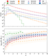 |
Fig. 1. Redshift distribution (top) and stellar mass as a function of redshift (bottom) of the simulated galaxies obtained with SPRITZ for the Euclid Deep Survey, colour-coded by their SED type (see the legend). Markers represent the median value in the redshift bin and shaded areas the corresponding 68% coverage interval. For details about the mass function distribution at different redshift ranges, we refer the reader to Bisigello et al. (2021). |
In this simulated catalogue, we also included photometry in additional filters, from Rubin and the Spitzer Infrared Array Camera (IRAC, Fazio et al. 2004), as these ancillary observations will be available to complement Euclid space-based data (Euclid Collaboration 2022a), at least for a fraction of the observed fields. It should be noted, however, that the IRAC photometry is affected by source confusion at faint magnitudes. Specifically, at IRAC/3.6μm > 22, a de-blending based on the available Euclid data (Euclid Collaboration 2022b) will be necessary when dealing with real observations. The expected 5σ and 2σ depths of the Euclid, Rubin and IRAC bands are reported in Table 1.
Depths of the filters considered in this work.
2.2.1. Photometric errors
In the SPRITZ lightcone used in this work, only the Euclid photometric bands have an associated observational uncertainty (i.e. the errors on the simulated magnitudes). We perturbed the Rubin and Spitzer fluxes to mimic realistic observations. In particular, the Rubin total photometric error has both a systematic and a random contribution and can be written as (Ivezić et al. 2019)
 (1)
(1)
where σrand is the random photometric error and σsys is the systematic one. Given that the Rubin telescope is designed to have a systematic error below 0.005 mag, we decided to neglect it in this work. The random photometric uncertainty can be written as a function of the magnitude (Ivezić et al. 2019):
 (2)
(2)
 (3)
(3)
where m5 is the 5σ depth (see Table 1) and γ is a parameter equal to 0.039 for the g, r, i, and z bands and 0.038 for u. The photometry for each galaxy in each Rubin filter was then derived by randomly sampling a Gaussian distribution with mean equal to the true value and standard deviation σrand.
Similarly, for the two Spitzer bands (IRAC/3.6 μm and IRAC/4.5 μm), we considered errors from Laigle et al. (2016) and parametrised them using Eqs. (2)–(3) with m5 as in Table 1 and γ = 0.038.
2.3. Photometric selections
The first step in our analysis was to validate the simulated Euclid Deep Field catalogue’s compatibility with a set of observed photometric diagnostics available from the literature, with a focus on high-z galaxies. The main focus in this work is the dusty and massive galaxy populations at 3 ≲ z ≲ 7. For their selection, we relied on the evolutionary H − [4.5] tracks of a set of theoretical galaxy SED templates for z > 3, assuming the colour cut-off suggested by Wang et al. (2016):
![Mathematical equation: $$ \begin{aligned} H - [4.5] > 2.25. \end{aligned} $$](/articles/aa/full_html/2024/05/aa48737-23/aa48737-23-eq4.gif) (4)
(4)
This colour was proposed to select old or dusty galaxies at z > 3. Objects satisfying this criterion are referred to as HIEROs. In particular, it was found that almost none of the spectroscopically confirmed LBGs at z > 3 satisfies this criterion. These are examples of the types of objects missed by conventional UV/optical surveys that we aim to recover with the future Euclid Deep Survey. Furthermore, based on the colour tracks of theoretical models and their photometric redshifts, HIEROs can be separated in two main classes:
![Mathematical equation: $$ \begin{aligned}&\mathrm{blue\,HIEROs,}&H-[4.5]>2(J-H)+1.45\,; \end{aligned} $$](/articles/aa/full_html/2024/05/aa48737-23/aa48737-23-eq5.gif) (5)
(5)
![Mathematical equation: $$ \begin{aligned}&\mathrm{red\,HIEROs,}&H-[4.5]\le 2(J-H)+1.45\,. \end{aligned} $$](/articles/aa/full_html/2024/05/aa48737-23/aa48737-23-eq6.gif) (6)
(6)
According to Wang et al. (2016), blue HIEROs are dominated by normal massive and dusty star forming galaxies at z ≳ 3. Red HIEROs, instead, include a mix of lower z ∼ 2 − 3 dusty star forming objects and passive galaxies at z ∼ 3 − 4. Passive galaxies are expected to be the most massive systems at any cosmic epoch, and are thus relevant for our study.
Figure 2 (left panel) shows the HE − [4.5]/JE − HE diagram for the Euclid Deep Survey simulated catalogue with 2 ≤ z ≤ 8 and fluxes brighter than their 5σ detection limits, coloured by redshift. To better highlight the different populations, in the top-right panel we report their redshift distributions: a clear difference arises between HIEROs and other objects, with 99% of HIEROs being at z > 3 and 43% of non-HIEROs being above the same redshift.
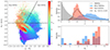 |
Fig. 2. HIEROs selection, redshift and extinction in the Simulated Euclid Deep Survey Catalogue. Left: HE − [4.5] versus JE − HE diagram for the simulated Euclid Deep survey catalogue (5σ depth) colour-coded by redshift. Top right: Redshift distribution of red HIEROs (red), blue HIEROs (blue), and galaxies with HE − [4.5]< 2.25 (grey). Bottom right: Optical extinction distribution of red HIEROs (red) and blue HIEROs (blue). We normalised each histogram to obtain an area equal to unity. |
The bottom-right panel shows, instead, the extinction properties for red and blue HIEROs (in terms of AV distributions). As expected, their red colours are mostly due to the presence of dust, with the bulk of AV ∼ 4 mag and spanning values up to 5.5 mag. We note that by selection both blue and red HIEROs include highly extinguished objects (Wang et al. 2016), so it is natural to observe consistent AV distributions (while keeping in mind that blue and red HIEROs peak at different cosmic epochs).
Given that in our simulation red HIEROs dominate the number densities of red sources at z ∼ 4, while blue HIEROs populate the higher redshift queue up to z ∼ 7–8, we included in the following discussion the study of the overall class of Euclid sources with H − [4.5]> 2.25, focusing on the 3 < z < 7 redshift range (where the bulk of HIEROs lye). To check the representativeness of our HIERO mock catalogue, we compared the overall number densities with the observations of Wang et al. (2016), who selected HIEROs with [4.5] < 24 over an area of 350 arcmin2 and detected a cleaned sample of 285 sources. Restricting our selection (i.e. requiring at least four detections at S/N > 2 in the considered bands; see Sect. 3.2.2) to the same magnitude limit of Wang et al. (2016), we identify 155 objects over the same area. However, if we mimic the Wang et al. (2016) selection by simply requiring a 5σ detection at 4.5μm, and [4.5]< 24, the number of predicted HIEROs increases to 425 (over 350 arcmin2). The variance on the predicted space densities, related to the assumed selection function, shows that the our mock catalogue provides a statistical sampling of the HIERO population consistent with the real world.
To understand the role of HIEROs in the stellar mass assembly, we report in Fig. 3 (black lines) the overall stellar mass function for galaxies in the redshift range 4 < z < 6 from SPRITZ, split in two z bins. The mass function limited to HIEROs is also reported (red lines), showing the dominant contribution of this population to the massive end of the stellar mass function at z > 4. Both at z = 4.5 and 5.5, HIEROs constitute approximately 93% of the galaxies with M* > 1011.5 M⊙ and 32% of the galaxies with M* > 1010.5 M⊙. The figure includes the observed mass function of HIEROs at z ∼ 4 − 5 from Wang et al. (2016), confirming the consistency of our model with the observations, within the uncertainties.
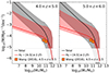 |
Fig. 3. Contribution of HIEROs to the galaxy stellar mass function in SPRITZ at z > 4 (red line). The grey and red shaded areas include the errors of the initial luminosity functions used to derive simulated galaxies and the uncertainties due to the high-z extrapolation (z > 3). The observed stellar mass function for HIEROs measured by Wang et al. (2016) at 4.5 < z < 5.5 is reported in both panels as filled orange squares. |
Finally, in Fig. 4 we show the most representative SED templates in SPRITZ for this population of galaxies, specifically the four most numerous templates used to generate red and blue HIEROs.
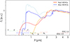 |
Fig. 4. The four most numerous SED templates used in SPRITZ for the generation of red HIEROs (red and orange) as considered at z = 4, and blue HIEROs (blue and light blue) at z = 5.5. The flux is in arbitrary units. We also show the wavelength coverage of the photometric bands considered in this work. |
3. Methods
In this section, we introduce the methods and the metrics that we used to estimate the capability of the future Euclid Space Telescope to identify high-redshift galaxies.
3.1. Gradient-boosted trees
We considered a gradient-boosting approach to independently predict both the redshifts and the SED types, based on the observed fluxes in different bands. This corresponds to a regression and a classification problem, respectively. Other methods have been proposed in the literature to classify different galaxy populations in Euclid (e.g. Bisigello et al. 2020, Euclid Collaboration 2023a) or to derive photometric redshifts (e.g. Euclid Collaboration 2020, Bisigello et al. in prep.), but none of these is focused on high-z galaxies.
The method proposed in this paper is a type of ensemble algorithm, in which the relationships between the features x and the target variables y = f(x) are learned by sequentially fitting new models: new decision trees (a representation of the decision tree model is shown in Fig. 5) are constructed to be maximally correlated with the negative gradient of the loss function associated with the ensemble. The loss function is chosen according to the task, while structural and learning parameters (referred to as hyperparameters) have to be tuned in a data-driven fashion.
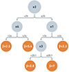 |
Fig. 5. Decision tree model. Grey nodes are called internal nodes and the orange ones, which represent the tree predictions, leaf nodes. Features are indicated with x1, x2, x3, or x4 and predictions with ỹ. Every internal node is labelled with an input feature. The arcs coming from a node labelled with an input feature (for example x4) to a leaf node (orange) are labelled with each of the possible values of the target feature (for example ỹ = 2.5 or |

The algorithm used in this work is implemented in the software package XGBoost (Chen & Guestrin 2016). Here we briefly summarise its main features while for more details we refer to the paper in which the library is presented or the online documentation1.
There are four main reasons to use gradient-boosted trees, and in particular XGBoost, in this work:
1. Execution speed: Generally, XGBoost is faster than back-propagation-based models (e.g. neural networks), and even than some other gradient-boosting implementations (Pafka 2015). In addition, and of particular interest for galaxy identification, its support for hardware acceleration makes the speed difference with any SED-fitting algorithm very advantageous (see Sect. 3.5).
2. Model performance: Gradient-boosting dominates structured and tabular datasets on both regression and classification predictive modelling problems. It is the go-to algorithm for competition winners on Kaggle2.
3. Decision-based splits: In the decision tree model, the splitting occurs at certain thresholds for every feature (see Fig. 5). This makes the model more robust to outliers and to the presence of only upper or lower limits in certain attributes, because it does not make any difference how far a point is from such thresholds.
4. Missing values handling: The dataset used in this work includes missing data (NaNs) in one or more of the features. Traditionally, to handle NaNs one can specify a fixed value to replace missing numbers, or impute them with either the mean or the median of that feature. It is obvious that this approach might not always be the best choice. XGBoost enhances the function class to learn the best way to handle missing values: the idea is to learn a ‘default direction’ for each node and guide the sample with missing values along the default directions. This approach can be seen as an implicit way of imputing missing numbers.
We might also have considered other recent gradient-boosting implementations, for example CatBoost (Prokhorenkova et al. 2017) or LightGBM (Ke et al. 2017), which should perform very similarly to XGBoost. However, a systematic comparison of different gradient-boosting libraries is beyond the scope of this work. We opted for XGBoost due to its longer presence in the field, which has allowed for a more mature development of features and a wider user community.
3.2. XGBoost hyperparameters
A hyperparameter is a parameter whose value is used to control the learning process, which, as a consequence, cannot be learned, but has to be set by the user by evaluating the machine performance while varying its value.
The most impactful XGBoost hyperparameters are as follows:
– The number of estimators refers to the number of gradient-boosted trees fitted during the learning process. Larger values lead to more complex models, which, however, are more prone to overfitting3.
– The learning rate is the rate at which new trees are added to the ensemble. Lower values lead to a slower addition of new trees, thus preventing (or at least slowing down) overfitting.
– The maximum depth refers to that of a tree. Increasing this value will make the model more complex and more likely to overfit.
– γ is defined as the minimum loss reduction required to make a further partition on a leaf node of the tree. The larger γ is, the more conservative the algorithm will be.
– λ is the L2 (squared norm) regularisation term on the weights. Increasing this value will make the model more conservative.
– The column sample by tree is the subsample ratio of columns when constructing each tree. Subsampling occurs once for every tree constructed.
The values used in this work and the optimisation method used to derive them are reported in Sect. 3.5.
3.3. Data preprocessing and feature engineering
Data preprocessing is a fundamental step in machine learning, since the quality of data greatly impacts the capability of a model to learn. Therefore, before feeding the data to the machine learning model and tuning its hyperparameters, we preprocessed it by performing feature engineering and data cleaning. To begin, the magnitude cut applied to the simulated Euclid lightcone was set to a depth of 2σ, and we defined magnitudes larger than their 2σ limit (see Table 1) as missing numbers.
In the following analysis, we considered only objects at 2 ≤ z ≤ 8. This selection yields a dataset with 6 304 179 galaxies. We did not consider galaxies at z < 2 since the official photo-z pipelines are very well optimised for identifying low-redshift galaxies (see e.g. Euclid Collaboration 2023b, 2020). By utilising them, we assumed that we would have a clean selection of high-redshift objects.
To test the validity of this assumption, an analysis addressing potential contamination from low-redshift sources in the selection of HIEROs candidates is presented in Appendix D. In the same appendix we also assess the contamination by brown dwarfs.
3.3.1. Features engineering
In this work, each element in the data refers to the simulated photometry of a particular galaxy. To provide more information for the objects, some derived features are also included: the more that is known about the SED of a galaxy, the better the inference will be. The number of features provided in the dataset is limited to 11 (four Euclid, five Rubin, and two IRAC bands; see Table 1); therefore, we decided to include some additional features to add more information for the training. In particular, we included the following features.
– Differences: Pairwise (without permutation) differences of the magnitudes.
– Ratios: Pairwise ratios between magnitudes without permutation. Even though they have no physical meaning, they are used because we empirically found that they help the training, increasing (albeit slightly) the performance.
– Errors: Parametric photometric errors associated with each band, as given by Eq. (2) (applied to the perturbed magnitudes). This parametrisation is also applied for the Euclid magnitudes even tough their uncertainties are provided in the catalogue, as these are computed analytically starting from the true flux, unaffected by photometric errors.
This process generates a total of 132 features, whose importance is reported and discussed in Appendix C.
3.3.2. Data cleaning
To have a more reliable set of measurements, only objects detected (i.e. S/N > 2) in at least four bands are used for estimating photometric redshifts; their counts for different z ranges are reported in Table 2 and the fraction of detections per band (computed after the cleaning procedure) in Table 3. The choice of going to such a low S/N is explained in Sect. 3.4. We remind the reader that the starting catalogue contains galaxies with at least one detection in a Euclid filter.
Counts per squared degree for objects detected in at least four bands.
Fraction of detections, i.e. S/N > 2, per considered band for objects detected in at least four bands.
This cleaning procedure removes roughly 18% of the initial data, yielding a total of 5 174 988 galaxies. To show how the redshift distribution is not strongly affected by the cleaning performed, the percentage reduction of objects in different redshift ranges is also reported in Table 2.
In the following photometric redshift estimation procedure, for bands with missing numbers (which replaced magnitudes fainter than their 2σ detection limits), 2σ magnitude lower limits are used (see Table 1). Missing colours and ratios of magnitudes are also replaced with the 2σ magnitudes lower limits of the missing band (if only one) instead of their upper or lower limit, or left missing (if both magnitudes are missing).
These choices were taken in order to avoid the contamination of detected colours and ratios with other lower or upper bounded ones; they furthermore provided slightly better performance. Some clarifying examples are shown in Table A.1.
3.4. Performance metrics
Three metrics were used to evaluate the redshift prediction performance (m indicates the number of objects in the sample, z the true redshift, and z̃ the model-predicted redshift), the root mean squared error (RMSE), the bias (⟨Δz⟩), and the normalised median absolute deviation (NMAD), and the and the catastrophic outlier fraction (OLF):
For spectral type classification, to evaluate the model we used a simple accuracy metric:
3.5. The training set
To train and evaluate the model, the dataset must be divided into two subsets. The first one, of size Ntrain, is used to fit the model and is referred to as the training set. The second, of size Ntest, is not used to train the model; instead, its input elements are provided to the model to make predictions. This second subset is referred to as the test set. The objective of such a division was to estimate the performance of the machine learning model on new data. This procedure is called a train-test split and depends on the percentage size of the training and test sets with respect to the initial dataset.
To ensure the model is trained effectively, in real-world observations a training set must be built with the most robust measurements and accurate redshift estimations available. The redshifts in a training set are thus required to be estimated spectroscopically or with very reliable photometry derived from a larger number of bands than those that will be available with Euclid + ancillary data. Consequently, as detailed in Sect. 3.2.2, we decided to extend our analyses to objects with S/N > 2, as in real observations these objects will be supplemented with additional information that compensates for such a low S/N.
While in practical applications one typically has limited control over the size of the training set Ntrain, when forecasting future surveys observations it is useful to assess what dimension of the training set is required to obtain a given prediction performance. In this first part, the minimum training set size required to obtain good test performance is found by performing a baseline XGBoost regression on different numbers of training points Ntrain and then comparing the results obtained.
Figure 6 shows the RMSE, OLF, and NMAD improvement (evaluated on a test set of 1 000 000 galaxies subdivided into different redshift ranges) for different training set sizes4, as a function of Ntrain/(Ntrain + Ntest). By analysing such curves, we came to the following conclusions:
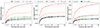 |
Fig. 6. Photometric redshift prediction performance improvement (as defined in Footnote 4) with respect to the metrics with the initial training set size (0.5% of the total number of galaxies), as a function of the training set size, evaluated on a sample of 1 000 000 test galaxies. From left to right we plot: the RMSE, OLF, and NMAD for different redshift intervals, as indicated in the legend. |
– All three performance metrics reported increase as Ntrain increases, as expected, but they begin to flatten for large Ntrain values. In general, the size of the training set required to obtain a certain precision depends on the diversity built into the dataset: for photometric redshifts it depends on the redshift range, meaning that the narrower the redshift range, the smaller the Ntrain required;
– The performance gain is in every case larger for higher redshift objects with respect to lower redshift ones; for example, the RMSE improvement for objects at 6 < z ≤ 7 becomes more than five times larger than the one for z ≤ 3 galaxies.
The number of detected galaxies at z < 4 is about four times the number of higher-z galaxies (see Table 2). This means that larger training sets are important to constraint the redshifts of rare objects: the majority of galaxies in the dataset (and, consequently, in the training set) are at low redshifts, so the training process gives more weight to the predictions for galaxies at low redshifts with respect to the other galaxies. Furthermore, for machine learning models, high-z objects are more difficult to identify than lower-z ones, given their larger photometric uncertainties.
To conclude, all the curves reported in Fig. 6 show an onset of a plateau at an Ntrain corresponding to roughly 10% of the data size. This 10%–90% train–test split will then be used in the following analyses.
3.6. Hyperparameter tuning and time performance
A Bayesian hyperparameters optimisation with cross-validation is then run on a training set large 10% of the total data size. The hyperparameters delivering the lowest RMSE thus found are reported in Table 4.
Best XGBoost hyperparameters.
Timed on a workstation with a 2.20 GHz Intel Xeon CPU and a 16 GB Tesla P100-PCIE GPU, an XGBoost regressor with these hyperparameters takes 70 s to train on a dataset with 517 498 samples and 132 features, and 40 s to estimate the redshift for the 4.6 million galaxies in the test set. To demonstrate the difference in speed with SED-fitting methods, performing this operation with LePHARE (Arnouts & Ilbert 2011) on similar hardware requires approximately 0.23 s per object (considering 463 680 different combinations of SED template, redshift, age and dust extinction). Estimating the photometric redshift for all the galaxies in the test set would then need approximately 12 days.
4. Results
During the testing phase, we set a higher significance threshold by considering only observations with at least one band having S/N > 5. This additional criterion, in conjunction with the requirement of at least four detections at S/N > 2 (see Sect. 3.2.2), aimed to minimise inclusions of spurious objects such as noise spikes, halos, and artefacts that would result from real observations. This removes roughly 21.728% of the initial test data Ntest, yielding a total of 3 645 481 galaxies. The results reported hereafter are thus relative to this dataset.
4.1. Photometric redshifts
The photo-z performance for the test set is summarised in Table B.1 and shown in Fig. 7.
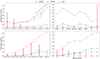 |
Fig. 7. XGBoost test set RMSE, OLF, and NMAD (starting from the upper-left panel and going clockwise) for different redshift intervals, SED types, numbers of missing bands, and i-band magnitudes. The grey curve shows the RMSE obtained by removing the two IRAC bands from the XGBoost input. The vertical pink bands indicate the fraction of objects belonging to the group with respect to the test set size. For details, refer to Table B.1. |
This figure clearly illustrates the trend of the performance metrics:
1. Top-left panel: The errors increase with redshift, as expected and noted in Sect. 3.4.
2. Bottom panels: The precision of the predicted redshift decreases for fainter objects, as these are usually found at higher z and they come with detections in fewer bands; this practically means the input features vectors contain less information to learn and infer from.
3. Top-right panel: The lowest errors (RMSE = 0.22) are obtained for elliptical galaxies, and the largest for AGN1, SF-AGN, and SBs (RMSE > 0.5). This behaviour may be related to their variability5 and (for SBs) their number density evolution with redshift: while ellipticals quickly drop from z = 2 to disappear at z ⪆ 3.5, SBs are observed at any redshift.
Furthermore, by removing the IRAC bands from the input features, we note (Fig. 7, top-left panel) how mid-IR data improves redshift estimation especially for z ≳ 4 galaxies.
4.2. Comparison with previous results
To give context to the results obtained, we compared them to previous photometric redshift performance, in a similar redshift range, as reported in Weaver et al. (2022, hereafter W22). There, the precision of the photometric redshifts obtained with LePHARE using 39 bands, and included in the COSMOS2020 catalogue, is assessed against spectroscopic ones over the Cosmic Evolution Survey (COSMOS, Scoville et al. 2007) field (0 < z < 6).
The photometric catalogues created in COSMOS, with their rich multi-wavelength coverage, have for years constituted the state of the art reference to predict the quality of photo-zs. Within the Euclid Collaboration (Euclid Collaboration 2020), this assessment has been done using the COSMOS2015 catalogue (Laigle et al. 2016). Improving on previous releases, the COSMOS2020 catalogue features significantly deeper optical, IR, and near-IR data and thus gains almost one order of magnitude in photometric redshift precision compared to its predecessor COSMOS2015.
Comparing the results reported in W22 and those obtained in this work using a gradient-boosting approach on the simulated Euclid Deep Survey catalogue, we find that even in the faintest 25 < i < 27 bin, gradient-boosting provides a lower NMAD (0.019 versus 0.044), and also a lower OLF (0.005 versus 0.204). Overall, the performance of the XGBoost method presented in this work is comparable to the performance of previous SED-fitting at each magnitude range, but our process is based on a notably smaller number of filters as inputs (i.e. 11 instead of 39).
It is important to remind the reader that our results are derived from simulated data, which is a simplified representation of reality, and therefore may not reflect actual performance accurately and could potentially overestimate it. The aim of this comparison is therefore to show that our performance is in line with previous studies without stressing much the one-to-one direct comparison.
To conclude this photo-z section, we estimate that in the range z > 6 the fraction of contaminants is relatively low, at 12%, while the completeness is around 72%. For comparison, Euclid Collaboration (2022c), using the same set of photometric bands (Euclid+ Rubin + Spitzer) and estimating with LePHARE the photometric redshifts of mock galaxies created from the Ultra Deep Survey with the VISTA telescope (UltraVISTA, McCracken et al. 2012), obtained at z > 6 a contamination fraction of 12% for bright UltraVISTA-like galaxies, with a z > 6 completeness of 95%. For fainter sources (25.3 ≤ HE < 27.0), contamination is more prevalent at 35%, with a z > 6 completeness of 88%. Our smaller completeness and contaminant fractions are mostly due to the unbalanced redshift distribution in the dataset (and consequently in the training set), as pointed out in Sect. 3.4. In fact, objects at z > 6 are systematically placed at lower redshifts, as their average offset z̃−z is ≈ − 0.483, while for objects at z < 6 it is ≈0.001. However, this paper focuses mainly at 3 < z < 7 , where the XGBoost performance is better, with a completeness of 89.3% and a contaminant fraction of 7.73%.
4.3. SED type classification
We also performed an independent experiment, applying the same methodology with the aim of recovering the classification of the spectral class of each source. The prior knowledge on the redshift derived as in the previous sections is ignored here.
When used as a classifier, when a feature vector is fed to it, the XGBoost output is a vector of probabilities, in this case with eight entries, each one corresponding to an SED type. The predicted class is thus the one corresponding to the maximum value. Each simulated galaxy is assigned an SED template taken from a set of 35 templates, divided into eight spectral types, as reported in Sect. 2.1.
Since the XGBoost input data and the train-test split used are the same as in the photometric redshift estimation, we used the same hyperparameters (Table 4). The accuracy obtained on the test set is 96.8%, meaning that 3 529 289 galaxies out of 3 645 481 are correctly classified. Some significant misclassifications (see the confusion matrix in Fig. 8) are explained by considering the nature of the SEDs and the photometry available. For example, it is reasonable that AGN2 and SB-AGN, both obscured in the optical, are misclassified as SBs, since it would be necessary to have spectroscopic data or photometric observations in the mid-IR (rest-frame) and X-ray, to identify their AGN nature.
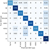 |
Fig. 8. Test set confusion matrix for SED type classification. Each row of the matrix represents the fraction of samples in an actual SED type, while each column represents the fraction of samples in a predicted SED type. The superimposed numbers indicate the fraction of objects of a class in that particular position. For example, considering the second row (SBs): 96% of SBs are correctly classified as such, 3% as SB-AGN, and 1% as Irregular. |
The distribution of the maximum probability per object for correct and wrong classifications is shown in Fig. 9. While for the mistakenly classified samples it is a rather flat distribution, for correct predictions it is strongly peaked at values of maximum probability larger than ≈0.95. This means it is possible to improve the spectral type prediction accuracy even more, by simply considering objects with large maximum probability, while losing a negligible number of correct predictions. For example, by keeping only objects with maximum probability > 0.8, the number of misclassified objects goes down by 61%, while dropping only 3.7% of the correctly classified ones. The resulting accuracy is 98.7%.
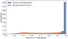 |
Fig. 9. Maximum probability distribution for correct (blue) and wrong (orange) classifications. The sum of the heights of each histogram is one. |
4.4. Identifying HIEROs
Having determined the general framework for the estimations of photometric redshifts and spectral types, in this section we present the results of the approach applied to the most relevant population in our study, namely red and massive galaxies at distances greater than z ≈ 3. We selected them as HIEROs (Eq. (4) and Fig. 2).
As these massive galaxies are challenging to spectroscopically confirm, to obtain a more realistic estimate of the identification performance of this population, we trained the gradient-boosting algorithm with a more realistic spectroscopic completeness: we utilised the training set as described in the previous sections but retaining only 500 HIEROs, which accounts for approximately 1/46 of the total number of HIEROs that would be available. We consider this to be conservative approach since:
-
We assume that a robust sample of HIERO that we could use as training set will be available in the COSMOS field, thanks to the very precise and accurate photometric redshifts derived from the already available and future multi-wavelength observations (W22; Casey et al. 2023).
-
We assume that in the next few years we will have access to spectroscopic redshifts for HIEROs thanks to JWST, as there are already photometric candidates suitable for follow-up (i.e. 138 objects similar to HIEROs in an area of 38.8 arcmin2 Pérez-González et al. 2023).
As there is clearly some stochasticity in the sampling of the HIEROs in the training set, the results reported are the average across multiple runs.
In Table 5 their identification performance is shown in terms of photo-z and SED type classification. The regression performance is compared to that reported in Wang et al. (2016), where the NMAD is approximately 0.1. Even for this population, the performance obtained in this work (HIEROs NMAD = 0.068) is encouraging, especially for the brightest galaxies (HE ≤ 26), as shown in Figs. 10 and 11. Clearly, the advantage of the Euclid Deep Fields survey will be the HIEROs’ much larger statistical relevance compared to previous surveys.
Redshift and spectral type prediction performance for HIEROs.
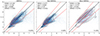 |
Fig. 10. Contour plot of XGBoost predictions (z̃) versus catalogue redshifts (z) coloured by density in the (z,z̃) space for HIEROs (left panel), red HIEROs (middle panel), and blue HIEROs (right panel), all of which have HE ≤ 26. Lighter contour colours indicate higher densities. The dashed red lines show z̃ = z ± 0.15(1 + z). The percentage of objects with respect to Ntest is indicated in the bottom-right corner of each panel. |
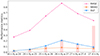 |
Fig. 11. RMSE, OLF, and NMAD values for HIEROs of different HE-band magnitudes. The vertical pink bands indicate the fraction of objects belonging to the group with respect to the total number of HIEROs. |
We also report in Table 6 the completeness and fraction of contaminants in different redshift ranges. The redshift range where we expect to find the vast majority of these objects (i.e. 3 ≤ z < 7) is complete at 99.4%, with a contaminant fraction of only 5%, mostly coming from higher-redshift galaxies.
Confusion matrix for photometric redshift ranges for HIEROs.
Lastly, the spectral type classification, although less accurate than for non-HIEROs (86.20% versus 97.20%), shows (Fig. 12) a similar confusion between classes to the classifications for all the objects in the catalogue (Fig. 8).
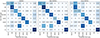 |
Fig. 12. SED type classification confusion matrix for HIEROs, red HIEROs, and blue HIEROs. The high confusion for ellipticals is explained by noting that there are only 20 of them in the HIERO selection (six in the red HIEROs and 14 in the blue HIEROs), none of them correctly identified. |
5. Summary and discussion
5.1. A new approach to identifying the most elusive and massive systems with Euclid at high z
In this work we have taken a photometric approach to predicting whether Euclid will provide enough information to resolve one of the key scientific unknowns in galaxy formation and evolution studies: the role of distant obscured galaxies in the buildup of today’s large-scale structures.
Such sources have proven to be elusive in optical surveys, and current near-IR surveys are deep enough to detect them only in very small sky areas. Since these optically faint objects are rare, large-area surveys that go to sufficient depths are necessary to provide a statistical census of such a population. Euclid will potentially provide all the ingredients to recover these missing galaxies at high redshifts (e.g. z > 3). However, it has been unclear if the photometric information it will deliver will be sufficient to identify and characterise them, given the lack of bright spectroscopic features observable by Euclid at these distances (i.e. λrest − frame < 0.5 μm).
Our goal was therefore to assess the capability of Euclid in combination with ancillary data to identify these distant obscured objects. We carried out the following analysis:
– We adopted the simulated Euclid Deep Fields catalogue from the SPRITZ simulation as a basis for our analysis and show that it includes a massive and dusty population, as selected by the criterion HE − [4.5]> 2.25. A total of 98% of these simulated objects (the HIEROs) are indeed at 3 < z < 7 and contribute significantly (≈93%) to the massive end of the stellar mass function at z > 4.
– We implemented a general, fast, and accurate machine learning technique optimised for z ≥ 2 galaxy identification, based on photometric data from Euclid, Rubin, and Spitzer, finding that only a ≈10% subset of the total observed galaxies with spectroscopic redshifts (or reliable photometric redshifts) is required to obtain a good performance (RMSE = 0.363, OLF = 0.061, ⟨Δz⟩= − 0.017, and NMAD = 0.039 over 2 ≤ z < 8). This photo-z precision is comparable to that of the COSMOS2020 catalogue, obtained with state-of-the-art traditional SED-fitting methods with almost four times the number of photometric bands.
– We applied the same methods for spectral type classification, distinguishing between eight different spectral types (i.e. spiral, SB, star-forming AGN, SB-AGN, type-1 AGN, type-2 AGN, elliptical, and irregular), obtaining an accuracy of 96.8%.
– We evaluated the identification performance for objects within the HIEROs selection and found a photo-z OLF = 0.123 and NMAD = 0.068; the SED classification accuracy is 86.2%. Evaluating only the brightest HIEROs (HE < 26), we obtained an OLF = 0.085, an NMAD = 0.055, and a 92.68% SED classification accuracy.
– We determined the completeness and the fraction of contaminants for the HIERO photo z. In the range 3 ≤ z < 7, we estimated a completeness of 99.4% and a contaminant fraction of 5%. The majority of the HIEROs are at z > 7.
All these results suggest that by leveraging Euclid, Rubin, and Spitzer photometric data, and by taking the approach described in this paper, it will be possible to constrain the contribution of the dusty and massive galaxies at z ≈ 3 − 7 to the mass functions and, hopefully, to the SFRD.
5.2. Future perspectives
Under suitable conditions, gradient-boosting (like many other supervised machine learning techniques) is a very competitive tool for photometric redshift and spectral type estimation. However, its successful application depends on the availability of a large enough training set that is representative of the populations under consideration. It is therefore most effective when applied to large photometric surveys, some of which include spectroscopic data for subsets of the photometric catalogues. One considerable problem for these methods is the difficulty in extrapolating to regions of the feature space not properly represented in the training data; the distribution of magnitudes and colours of the training set has to be as close as possible to those in the target set.
Lastly, the good performance demonstrated here relies heavily on the representativeness of the SPRITZ simulation with respect to the Euclid observations. It has been shown (Bisigello et al. 2021, 2022) that SPRITZ results are in agreement with a large set of observations at different wavelengths. However, the simulation also has some limitations. For example, the number of SED templates included in the simulation is limited, and results at number densities z > 3 are, though widely tested, mainly based on extrapolation. Therefore, the results shown here may be prone to biases or may be slightly optimistic compared to those that will be obtained once real data become available. To mitigate this limitation and enable a more robust forecast, future work could apply the methods of this paper to different simulated datasets, for example MAMBo (Mocks with Abundance Matching in Bologna; Girelli et al. 2020), and compare the results obtained with those of the official Euclid pipelines.
Furthermore, some additional strategies can be used to improve the predictions. The gradient-boosting algorithm can easily be extended to provide a probability distribution even on redshifts.
After applying the most effective photometric pipeline to real data, a promising selection of candidate galaxies will be obtained. To confirm their nature, spectroscopic follow-up will be necessary, for example via the Extremely Large Telescope, ALMA, or JWST.
Kaggle (https://www.kaggle.com/) is a community of data scientists and a place to find and publish datasets, explore and build models in a web environment, and participate in data science and machine learning competitions (with prizes).
Overfitting is the production of an analysis corresponding too closely to a particular dataset, and might thus fail to predict new observations reliably.
The improvement of a metric for a training set of size Ntrain, with respect to the initial training set size one, M0, is defined as M0 − M(Ntrain), where M(Ntrain) is the metric evaluated after training with Ntrain data points.
Data variability refers to how spread out a set of data is.
Acknowledgments
We thank Tao Wang for sharing his data for the stellar mass function for HIEROs. The Euclid Consortium acknowledges the European Space Agency and a number of agencies and institutes that have supported the development of Euclid, in particular the Academy of Finland, the Agenzia Spaziale Italiana, the Belgian Science Policy, the Canadian Euclid Consortium, the French Centre National d’Etudes Spatiales, the Deutsches Zentrum für Luft- und Raumfahrt, the Danish Space Research Institute, the Fundação para a Ciência e a Tecnologia, the Ministerio de Ciencia e Innovación, the National Aeronautics and Space Administration, the National Astronomical Observatory of Japan, the Netherlandse Onderzoekschool Voor Astronomie, the Norwegian Space Agency, the Romanian Space Agency, the State Secretariat for Education, Research and Innovation (SERI) at the Swiss Space Office (SSO), and the United Kingdom Space Agency. A complete and detailed list is available on the Euclid web site (http://www.euclid-ec.org).
References
- Abdalla, F. B., Banerji, M., Lahav, O., & Rashkov, V. 2011, MNRAS, 417, 1891 [NASA ADS] [CrossRef] [Google Scholar]
- Algera, H. S. B., Inami, H., Oesch, P. A., et al. 2023, MNRAS, 518, 6142 [Google Scholar]
- Arnouts, S., & Ilbert, O. 2011, Astrophysics Source Code Library [record ascl:1108.009] [Google Scholar]
- Ball, N. M., Brunner, R. J., Myers, A. D., et al. 2008, ApJ, 683, 12 [NASA ADS] [CrossRef] [Google Scholar]
- Barro, G., P\’{e}rez-Gonz\’{a}lez, P. G., Kocevski, D. D., et al. 2024, ApJ, 963, 128 [CrossRef] [Google Scholar]
- Barrufet, L., Oesch, P. A., Bouwens, R., et al. 2023a, MNRAS, 522, 3926 [NASA ADS] [CrossRef] [Google Scholar]
- Barrufet, L., Oesch, P. A., Weibel, A., et al. 2023b, MNRAS, 522, 449 [NASA ADS] [CrossRef] [Google Scholar]
- Benitez, N. 2000, ApJ, 536, 571 [CrossRef] [Google Scholar]
- Bian, F., Fan, X., Jiang, L., et al. 2013, ApJ, 774, 28 [Google Scholar]
- Bianchi, S., De Vis, P., Viaene, S., et al. 2018, A&A, 620, A112 [NASA ADS] [CrossRef] [EDP Sciences] [Google Scholar]
- Bisigello, L., Kuchner, U., Conselice, C. J., et al. 2020, MNRAS, 494, 2337 [NASA ADS] [CrossRef] [Google Scholar]
- Bisigello, L., Gruppioni, C., Calura, F., et al. 2021, PASA, 38, e064 [NASA ADS] [CrossRef] [Google Scholar]
- Bisigello, L., Vallini, L., Gruppioni, C., et al. 2022, A&A, 666, A193 [NASA ADS] [CrossRef] [EDP Sciences] [Google Scholar]
- Bisigello, L., Gandolfi, G., Grazian, A., et al. 2023, A&A, 676, A76 [NASA ADS] [CrossRef] [EDP Sciences] [Google Scholar]
- Boogaard, L. A., Decarli, R., Walter, F., et al. 2023, ApJ, 945, 111 [NASA ADS] [CrossRef] [Google Scholar]
- Brandt, W. N., Ni, Q., Yang, G., et al. 2018, ArXiv e-prints [arXiv:1811.06542] [Google Scholar]
- Burrows, A., Sudarsky, D., & Hubeny, I. 2006, ApJ, 640, 1063 [Google Scholar]
- Capak, P., Arendt, R., Arnouts, S., et al. 2016, Spitzer Proposal ID 13058, https://ui.adsabs.harvard.edu/abs/2016sptz.prop13058C [Google Scholar]
- Caputi, K. I., Caminha, G. B., Fujimoto, S., et al. 2021, ApJ, 908, 146 [NASA ADS] [CrossRef] [Google Scholar]
- Casey, C. M., Kartaltepe, J. S., Drakos, N. E., et al. 2023, ApJ, 954, 31 [NASA ADS] [CrossRef] [Google Scholar]
- Chen, T., & Guestrin, C. 2016, ArXiv e-prints [arXiv:1603.02754] [Google Scholar]
- Cropper, M., Pottinger, S., Niemi, S., et al. 2016, SPIE Conf. Ser., 9904, 99040Q [NASA ADS] [Google Scholar]
- Daddi, E., Dannerbauer, H., Stern, D., et al. 2009, ApJ, 694, 1517 [Google Scholar]
- Enia, A., Talia, M., Pozzi, F., et al. 2022, ApJ, 927, 204 [NASA ADS] [CrossRef] [Google Scholar]
- Euclid Collaboration (Desprez, G., et al.) 2020, A&A, 644, A31 [EDP Sciences] [Google Scholar]
- Euclid Collaboration (Scaramella, R., et al.) 2022a, A&A, 662, A112 [NASA ADS] [CrossRef] [EDP Sciences] [Google Scholar]
- Euclid Collaboration (Moneti, A., et al.) 2022b, A&A, 658, A126 [NASA ADS] [CrossRef] [EDP Sciences] [Google Scholar]
- Euclid Collaboration (van Mierlo, S. E., et al.) 2022c, A&A, 666, A200 [NASA ADS] [CrossRef] [EDP Sciences] [Google Scholar]
- Euclid Collaboration (Schirmer, M., et al.) 2022d, A&A, 662, A92 [NASA ADS] [CrossRef] [EDP Sciences] [Google Scholar]
- Euclid Collaboration (Humphrey, A., et al.) 2023a, A&A, 671, A99 [NASA ADS] [CrossRef] [EDP Sciences] [Google Scholar]
- Euclid Collaboration (Bisigello, L., et al.) 2023b, MNRAS, 520, 3529 [NASA ADS] [CrossRef] [Google Scholar]
- Fazio, G. G., Hora, J. L., Allen, L. E., et al. 2004, ApJS, 154, 10 [Google Scholar]
- Foley, R. J., Koekemoer, A. M., Spergel, D. N., et al. 2018, ArXiv e-prints [arXiv:1812.00514] [Google Scholar]
- Frayer, D. T., Smail, I., Ivison, R. J., & Scoville, N. Z. 2000, AJ, 120, 1668 [NASA ADS] [CrossRef] [Google Scholar]
- Fujimoto, S., Kohno, K., Ouchi, M., et al. 2023, ApJS, submitted [arXiv:2303.01658] [Google Scholar]
- Girelli, G., Pozzetti, L., Bolzonella, M., et al. 2020, A&A, 634, A135 [NASA ADS] [CrossRef] [EDP Sciences] [Google Scholar]
- Gruppioni, C., Pozzi, F., Andreani, P., et al. 2010, A&A, 518, L27 [NASA ADS] [CrossRef] [EDP Sciences] [Google Scholar]
- Gruppioni, C., Pozzi, F., Rodighiero, G., et al. 2013, MNRAS, 432, 23 [Google Scholar]
- Gruppioni, C., Béthermin, M., Loiacono, F., et al. 2020, A&A, 643, A8 [NASA ADS] [CrossRef] [EDP Sciences] [Google Scholar]
- Huang, J. S., Rigopoulou, D., Magdis, G., et al. 2014, ApJ, 784, 52 [Google Scholar]
- Ibata, R. A., McConnachie, A., Cuillandre, J.-C., et al. 2017, ApJ, 848, 128 [Google Scholar]
- Ilbert, O., Capak, P., Salvato, M., et al. 2009, ApJ, 690, 1236 [NASA ADS] [CrossRef] [Google Scholar]
- Ivezić, Z., Kahn, S. M., Tyson, J. A., et al. 2019, ApJ, 873, 111 [NASA ADS] [CrossRef] [Google Scholar]
- Ke, G., Meng, Q., Finely, T., et al. 2017, Advances in Neural Information Processing Systems 30 (NIP 2017) [Google Scholar]
- Laigle, C., McCracken, H. J., Ilbert, O., et al. 2016, ApJS, 224, 24 [Google Scholar]
- Laureijs, R., Amiaux, J., Arduini, S., et al. 2011, ArXiv e-prints [arXiv:1110.3193] [Google Scholar]
- Liu, R. H., Hill, R., Scott, D., et al. 2019, MNRAS, 489, 1770 [NASA ADS] [CrossRef] [Google Scholar]
- Loiacono, F., Decarli, R., Gruppioni, C., et al. 2021, A&A, 646, A76 [EDP Sciences] [Google Scholar]
- Lundberg, S. M., Erion, G., Chen, H., et al. 2020, Nat. Mach. Intell., 2, 2522 [Google Scholar]
- Madau, P., & Dickinson, M. 2014, ARA&A, 52, 415 [Google Scholar]
- Masters, D. C., Stern, D. K., Cohen, J. G., et al. 2019, ApJ, 877, 81 [Google Scholar]
- McCracken, H. J., Milvang-Jensen, B., Dunlop, J., et al. 2012, A&A, 544, A156 [NASA ADS] [CrossRef] [EDP Sciences] [Google Scholar]
- Novak, M., Smolč ić, V., Delhaize, J., et al. 2017, A&A, 602, A5 [NASA ADS] [CrossRef] [EDP Sciences] [Google Scholar]
- Oke, J. B., & Gunn, J. E. 1983, ApJ, 266, 713 [NASA ADS] [CrossRef] [Google Scholar]
- Pafka, S. 2015, Benchmarking Random Forest Implementations, https://www.r-bloggers.com/2015/05/benchmarking-random-forest-implementations/">http://www.w3.org/1999/xlink">https://www.r-bloggers.com/2015/05/benchmarking-random-forest-implementations/ [Google Scholar]
- Pasquet, J., Bertin, E., Treyer, M., Arnouts, S., & Fouchez, D. 2019, A&A, 621, A26 [NASA ADS] [CrossRef] [EDP Sciences] [Google Scholar]
- Pérez-González, P. G., Barro, G., Annunziatella, M., et al. 2023, ApJ, 946, L16 [CrossRef] [Google Scholar]
- Polletta, M., Tajer, M., Maraschi, L., et al. 2007, ApJ, 663, 81 [NASA ADS] [CrossRef] [Google Scholar]
- Prokhorenkova, L., Gusev, G., Vorobev, A., Veronika Dorogush, A., & Gulin, A. 2017, ArXiv e-prints [arXiv:1706.09516] [Google Scholar]
- Riechers, D. A., Pavesi, R., Sharon, C. E., et al. 2019, ApJ, 872, 7 [Google Scholar]
- Rieke, G. H., Alonso-Herrero, A., Weiner, B. J., et al. 2009, ApJ, 692, 556 [NASA ADS] [CrossRef] [Google Scholar]
- Rodighiero, G., Bisigello, L., Iani, E., et al. 2023, MNRAS, 518, L19 [Google Scholar]
- Scoville, N., Aussel, H., Brusa, M., et al. 2007, ApJS, 172, 1 [Google Scholar]
- Smail, I., Dudzevičiūt\.{e}, U., Stach, S. M., et al. 2021, MNRAS, 502, 3426 [NASA ADS] [CrossRef] [Google Scholar]
- Sun, F., Egami, E., Pérez-González, P. G., et al. 2021, ApJ, 922, 114 [NASA ADS] [CrossRef] [Google Scholar]
- Talia, M., Cimatti, A., Giulietti, M., et al. 2021, ApJ, 909, 23 [NASA ADS] [CrossRef] [Google Scholar]
- Topping, M. W., Stark, D. P., Endsley, R., et al. 2022, MNRAS, 516, 975 [NASA ADS] [CrossRef] [Google Scholar]
- van Dokkum, P. G., Quadri, R., Marchesini, D., et al. 2006, ApJ, 638, L59 [NASA ADS] [CrossRef] [Google Scholar]
- Wang, T., Elbaz, D., Schreiber, C., et al. 2016, ApJ, 816, 84 [Google Scholar]
- Wang, T., Schreiber, C., Elbaz, D., et al. 2019, Nature, 572, 211 [Google Scholar]
- Weaver, J. R., Kauffmann, O. B., Ilbert, O., et al. 2022, ApJS, 258, 11 [NASA ADS] [CrossRef] [Google Scholar]
- Williams, C. C., Labbe, I., Spilker, J., et al. 2019, ApJ, 884, 154 [Google Scholar]
- Xiao, M. Y., Elbaz, D., Gómez-Guijarro, C., et al. 2023, A&A, 672, A18 [NASA ADS] [CrossRef] [EDP Sciences] [Google Scholar]
Appendix A: Missing detection handling
We show some clarifying examples of the handling of missing detections used in this work in Table A.1.
Handling of missing detections.
Appendix B: Photo-z performance
Here we report the detailed XGBoost results for photometric redshifts (evaluated on the test set), for different redshift bins, SED types, i-band AB magnitudes, and numbers of missing detections (shown graphically in Fig. 7).
XGBoost prediction performance.
Appendix C: Photo-z feature importance
Figure C.1 shows the most important features for redshift estimation (evaluated on the test set) for HIEROs and other objects, in terms of Shapley values (Lundberg et al. 2020). These can be both positive and negative, and indicate the contribution of every feature to the model output, as for every data point the sum of its Shapley values is the predicted redshift. Here the sum of the modulus of these values is normalised to one.
While the redshift prediction is mostly based on colours and magnitude ratios, the feature importance order of the two populations is quite different, with the HIEROs redshift estimates being more strongly reliant on the near-IR magnitudes. The colours and ratios of the same magnitude pairs are ranked closely. We note, however, the number of missing detections per band (Table 3) and the consequent reduced variability of the magnitudes, which clearly influences the importance.
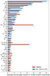 |
Fig. C.1. Feature rankings from the XGBoost model for HIEROs (red) and other objects (blue). We used the average of the absolute value of the normalised (by predicted redshift) Shapley values. This corresponds to the average percentage impact on model outputs. For example, on average, 8% of the model output for HIEROs is based on the HE − [4.5] colour, while for other objects the impact of this feature is only around 2%. |
Appendix D: Contaminants analysis
Throughout the paper, we considered only objects at z > 2, under the assumption that the selection of high-redshift objects from official photo-z pipelines would yield a clean dataset. In this appendix we analyse potential contamination issues from low-redshift (z < 2) sources, as well as brown dwarfs, in the selection of 3 < z < 7 HIEROs candidates.
To address the first concern, we applied a dedicated binary classifier using the same XGBoost algorithm and input features as described in the main body of the paper (see Sect. 4.2), with the goal of differentiating between objects at z < 2 and z > 2. This classifier is trained on a dataset comprehending objects down to z = 0 and 500 HIEROs (see Sect. 4.3). This training set consisted of 2 815 072 galaxies, the vast majority of which are at z < 2 (see, for example, Fig. 1, top panel).
The objective was to estimate the degree of contamination from low-z sources in the HIEROs selection (Eq. 4), essentially quantifying the number of galaxies with z < 2 that both fit within the colour-colour selection and that are predicted by the classifier at z > 2. We report the completeness and fraction of contaminants obtained from this analysis in Table D.1, reminding the reader that in the testing phase we consider only observations with at least four bands with S/N > 2 and at least one band with S/N > 5. These results underscore the classifier’s effectiveness in distinguishing between HE − [4.5]> 2.25 sources with redshifts above and below 2, showcasing high completeness at z > 2 (98.9%) and high purity, thereby minimising the risk of contamination (kept at only 1.1%).
Confusion matrix for photometric redshift ranges for HIEROs.
To assess the contamination by brown dwarfs, we simulated Euclid magnitudes based on the models of L and T dwarf from Burrows et al. (2006). These templates have effective temperatures ranging from 700 K to 2300 K, metallicities from [Fe/H]=−0.5 to 0.5, and gravities from 104.5 to 105.5 cm s−2. We did not simulate their spatial distribution, as this goes beyond the scope of this paper, but we derived magnitudes assuming they are located from 1 to 288 pc away from us, with steps of 1 pc. At larger distances, all brown dwarfs models correspond to S/N < 3 in all Euclid filter. We kept all mocks that results in a S/N > 3 in at least one Euclid filter, for a total of 33 866 simulated brown dwarfs. We then scattered their magnitudes using the same procedure reported in Sec. 2.2. We find that fewer than 1% of these brown dwarfs fall into the selection HE − [4.5]> 2.25 and thus the contamination from these sources in the HIEROs selection (applied to all objects in our catalogue with z > 2) is below 0.01%.
Consequently, we argue that the conclusions drawn in the main body of the paper remain largely unaffected even with the possible inclusion of z < 2 galaxies and brown dwarfs in the analysis.
Appendix E: Identifying HIEROs with shallower Rubin depths
The analysis presented in this work assumes Rubin depths after 10 years of observations. To evaluate the efficacy of our search for the reddest high-redshift galaxies before that time, we run the same tests described above with shallower depths (Table E.1), corresponding to one and four years of Rubin observations (Brandt et al. 2018). In all our runs, we considered 500 HIEROs in the training set.
As expected, the photo-z performance improves with each passing year, while also benefiting from a larger sample of HIEROs in the test set. The decrease in RMSE and ⟨Δz⟩ from year one to year 10 is a clear indication that the accuracy of the predictions has improved significantly over time. However, the most notable improvement is in the catastrophic OLF metric, which decreased from 0.254 in year one to 0.141 in year 10. This is a significant improvement, and it suggests that deeper observations are particularly important in reducing exceptionally wrong predictions.
Expected 5σRubin depths after one and four years of observations.
Redshift prediction performance for HIEROs obtained considering Rubin depths after one and four years of observations.
Appendix F: Rubin/y
We did not include in our analysis the Rubin/y band (2σ depth of 27.2 mag), as it was determined to have negligible impact on our results. We address this point by showing in Table F.1 the improvement in performance between the dataset with and without the Rubin/y band. This results demonstrate that the inclusion of this band yields little improvement on our results across most redshifts and magnitude intervals.
XGBoost improvement in RMSE, OLF, and NMAD with the inclusion of the Rubin/y band.
All Tables
Fraction of detections, i.e. S/N > 2, per considered band for objects detected in at least four bands.
Redshift prediction performance for HIEROs obtained considering Rubin depths after one and four years of observations.
XGBoost improvement in RMSE, OLF, and NMAD with the inclusion of the Rubin/y band.
All Figures
|
Fig. 1. Redshift distribution (top) and stellar mass as a function of redshift (bottom) of the simulated galaxies obtained with SPRITZ for the Euclid Deep Survey, colour-coded by their SED type (see the legend). Markers represent the median value in the redshift bin and shaded areas the corresponding 68% coverage interval. For details about the mass function distribution at different redshift ranges, we refer the reader to Bisigello et al. (2021). |
| In the text | |
|
Fig. 2. HIEROs selection, redshift and extinction in the Simulated Euclid Deep Survey Catalogue. Left: HE − [4.5] versus JE − HE diagram for the simulated Euclid Deep survey catalogue (5σ depth) colour-coded by redshift. Top right: Redshift distribution of red HIEROs (red), blue HIEROs (blue), and galaxies with HE − [4.5]< 2.25 (grey). Bottom right: Optical extinction distribution of red HIEROs (red) and blue HIEROs (blue). We normalised each histogram to obtain an area equal to unity. |
| In the text | |
|
Fig. 3. Contribution of HIEROs to the galaxy stellar mass function in SPRITZ at z > 4 (red line). The grey and red shaded areas include the errors of the initial luminosity functions used to derive simulated galaxies and the uncertainties due to the high-z extrapolation (z > 3). The observed stellar mass function for HIEROs measured by Wang et al. (2016) at 4.5 < z < 5.5 is reported in both panels as filled orange squares. |
| In the text | |
|
Fig. 4. The four most numerous SED templates used in SPRITZ for the generation of red HIEROs (red and orange) as considered at z = 4, and blue HIEROs (blue and light blue) at z = 5.5. The flux is in arbitrary units. We also show the wavelength coverage of the photometric bands considered in this work. |
| In the text | |
|
Fig. 5. Decision tree model. Grey nodes are called internal nodes and the orange ones, which represent the tree predictions, leaf nodes. Features are indicated with x1, x2, x3, or x4 and predictions with ỹ. Every internal node is labelled with an input feature. The arcs coming from a node labelled with an input feature (for example x4) to a leaf node (orange) are labelled with each of the possible values of the target feature (for example ỹ = 2.5 or |
| In the text | |
|
Fig. 6. Photometric redshift prediction performance improvement (as defined in Footnote 4) with respect to the metrics with the initial training set size (0.5% of the total number of galaxies), as a function of the training set size, evaluated on a sample of 1 000 000 test galaxies. From left to right we plot: the RMSE, OLF, and NMAD for different redshift intervals, as indicated in the legend. |
| In the text | |
|
Fig. 7. XGBoost test set RMSE, OLF, and NMAD (starting from the upper-left panel and going clockwise) for different redshift intervals, SED types, numbers of missing bands, and i-band magnitudes. The grey curve shows the RMSE obtained by removing the two IRAC bands from the XGBoost input. The vertical pink bands indicate the fraction of objects belonging to the group with respect to the test set size. For details, refer to Table B.1. |
| In the text | |
|
Fig. 8. Test set confusion matrix for SED type classification. Each row of the matrix represents the fraction of samples in an actual SED type, while each column represents the fraction of samples in a predicted SED type. The superimposed numbers indicate the fraction of objects of a class in that particular position. For example, considering the second row (SBs): 96% of SBs are correctly classified as such, 3% as SB-AGN, and 1% as Irregular. |
| In the text | |
|
Fig. 9. Maximum probability distribution for correct (blue) and wrong (orange) classifications. The sum of the heights of each histogram is one. |
| In the text | |
|
Fig. 10. Contour plot of XGBoost predictions (z̃) versus catalogue redshifts (z) coloured by density in the (z,z̃) space for HIEROs (left panel), red HIEROs (middle panel), and blue HIEROs (right panel), all of which have HE ≤ 26. Lighter contour colours indicate higher densities. The dashed red lines show z̃ = z ± 0.15(1 + z). The percentage of objects with respect to Ntest is indicated in the bottom-right corner of each panel. |
| In the text | |
|
Fig. 11. RMSE, OLF, and NMAD values for HIEROs of different HE-band magnitudes. The vertical pink bands indicate the fraction of objects belonging to the group with respect to the total number of HIEROs. |
| In the text | |
|
Fig. 12. SED type classification confusion matrix for HIEROs, red HIEROs, and blue HIEROs. The high confusion for ellipticals is explained by noting that there are only 20 of them in the HIERO selection (six in the red HIEROs and 14 in the blue HIEROs), none of them correctly identified. |
| In the text | |
|
Fig. C.1. Feature rankings from the XGBoost model for HIEROs (red) and other objects (blue). We used the average of the absolute value of the normalised (by predicted redshift) Shapley values. This corresponds to the average percentage impact on model outputs. For example, on average, 8% of the model output for HIEROs is based on the HE − [4.5] colour, while for other objects the impact of this feature is only around 2%. |
| In the text | |
Current usage metrics show cumulative count of Article Views (full-text article views including HTML views, PDF and ePub downloads, according to the available data) and Abstracts Views on Vision4Press platform.
Data correspond to usage on the plateform after 2015. The current usage metrics is available 48-96 hours after online publication and is updated daily on week days.
Initial download of the metrics may take a while.