| Issue |
A&A
Volume 691, November 2024
|
|
|---|---|---|
| Article Number | A175 | |
| Number of page(s) | 26 | |
| Section | Extragalactic astronomy | |
| DOI | https://doi.org/10.1051/0004-6361/202451425 | |
| Published online | 13 November 2024 | |
Euclid preparation
LI. Forecasting the recovery of galaxy physical properties and their relations with template-fitting and machine-learning methods
1
Dipartimento di Fisica e Astronomia “Augusto Righi” - Alma Mater Studiorum Università di Bologna, via Piero Gobetti 93/2, 40129 Bologna, Italy
2
INAF-Osservatorio di Astrofisica e Scienza dello Spazio di Bologna, Via Piero Gobetti 93/3, 40129 Bologna, Italy
3
Instituto de Astrofísica e Ciências do Espaço, Universidade do Porto, CAUP, Rua das Estrelas, PT4150-762 Porto, Portugal
4
DTx – Digital Transformation CoLAB, Building 1, Azurém Campus, University of Minho, 4800-058 Guimarães, Portugal
5
Faculdade de Ciências da Universidade do Porto, Rua do Campo de Alegre, 4150-007 Porto, Portugal
6
Department of Astronomy, University of Geneva, ch. d’Ecogia 16, 1290 Versoix, Switzerland
7
INAF, Istituto di Radioastronomia, Via Piero Gobetti 101, 40129 Bologna, Italy
8
Dipartimento di Fisica e Astronomia “G. Galilei”, Università di Padova, Via Marzolo 8, 35131 Padova, Italy
9
INAF-Osservatorio Astronomico di Capodimonte, Via Moiariello 16, 80131 Napoli, Italy
10
INFN section of Naples, Via Cinthia 6, 80126 Napoli, Italy
11
INAF-Osservatorio Astronomico di Trieste, Via G. B. Tiepolo 11, 34143 Trieste, Italy
12
Dipartimento di Fisica e Astronomia, Università di Firenze, via G. Sansone 1, 50019 Sesto Fiorentino, Firenze, Italy
13
INAF-Osservatorio Astrofisico di Arcetri, Largo E. Fermi 5, 50125 Firenze, Italy
14
INAF-Osservatorio Astronomico di Padova, Via dell’Osservatorio 5, 35122 Padova, Italy
15
Instituto de Astrofísica de Canarias (IAC); Departamento de Astrofísica, Universidad de La Laguna (ULL), 38200 La Laguna, Tenerife, Spain
16
Institute of Space Sciences (ICE, CSIC), Campus UAB, Carrer de Can Magrans, s/n, 08193 Barcelona, Spain
17
Université Paris-Saclay, CNRS, Institut d’astrophysique spatiale, 91405 Orsay, France
18
ESAC/ESA, Camino Bajo del Castillo, s/n., Urb. Villafranca del Castillo, 28692 Villanueva de la Cañada, Madrid, Spain
19
School of Mathematics and Physics, University of Surrey, Guildford, Surrey GU2 7XH, UK
20
INAF-Osservatorio Astronomico di Brera, Via Brera 28, 20122 Milano, Italy
21
IFPU, Institute for Fundamental Physics of the Universe, via Beirut 2, 34151 Trieste, Italy
22
INFN, Sezione di Trieste, Via Valerio 2, 34127 Trieste, TS, Italy
23
SISSA, International School for Advanced Studies, Via Bonomea 265, 34136 Trieste, TS, Italy
24
Dipartimento di Fisica e Astronomia, Università di Bologna, Via Gobetti 93/2, 40129 Bologna, Italy
25
INFN-Sezione di Bologna, Viale Berti Pichat 6/2, 40127 Bologna, Italy
26
Max Planck Institute for Extraterrestrial Physics, Giessenbachstr. 1, 85748 Garching, Germany
27
Universitäts-Sternwarte München, Fakultät für Physik, Ludwig-Maximilians-Universität München, Scheinerstrasse 1, 81679 München, Germany
28
INAF-Osservatorio Astrofisico di Torino, Via Osservatorio 20, 10025 Pino Torinese (TO), Italy
29
Dipartimento di Fisica, Università di Genova, Via Dodecaneso 33, 16146 Genova, Italy
30
INFN-Sezione di Genova, Via Dodecaneso 33, 16146 Genova, Italy
31
Department of Physics “E. Pancini”, University Federico II, Via Cinthia 6, 80126 Napoli, Italy
32
Dipartimento di Fisica, Università degli Studi di Torino, Via P. Giuria 1, 10125 Torino, Italy
33
INFN-Sezione di Torino, Via P. Giuria 1, 10125 Torino, Italy
34
INAF-IASF Milano, Via Alfonso Corti 12, 20133 Milano, Italy
35
Centro de Investigaciones Energéticas, Medioambientales y Tecnológicas (CIEMAT), Avenida Complutense 40, 28040 Madrid, Spain
36
Port d’Informació Científica, Campus UAB, C. Albareda s/n, 08193 Bellaterra (Barcelona), Spain
37
Institute for Theoretical Particle Physics and Cosmology (TTK), RWTH Aachen University, 52056 Aachen, Germany
38
Institut d’Estudis Espacials de Catalunya (IEEC), Edifici RDIT, Campus UPC, 08860 Castelldefels, Barcelona, Spain
39
INAF-Osservatorio Astronomico di Roma, Via Frascati 33, 00078 Monteporzio Catone, Italy
40
Dipartimento di Fisica e Astronomia “Augusto Righi” - Alma Mater Studiorum Università di Bologna, Viale Berti Pichat 6/2, 40127 Bologna, Italy
41
Instituto de Astrofísica de Canarias, Calle Vía Láctea s/n, 38204 San Cristóbal de La Laguna, Tenerife, Spain
42
Institute for Astronomy, University of Edinburgh, Royal Observatory, Blackford Hill, Edinburgh EH9 3HJ, UK
43
Jodrell Bank Centre for Astrophysics, Department of Physics and Astronomy, University of Manchester, Oxford Road, Manchester M13 9PL, UK
44
European Space Agency/ESRIN, Largo Galileo Galilei 1, 00044 Frascati, Roma, Italy
45
Université Claude Bernard Lyon 1, CNRS/IN2P3, IP2I Lyon, UMR 5822, Villeurbanne F-69100, France
46
Institute of Physics, Laboratory of Astrophysics, Ecole Polytechnique Fédérale de Lausanne (EPFL), Observatoire de Sauverny, 1290 Versoix, Switzerland
47
UCB Lyon 1, CNRS/IN2P3, IUF, IP2I Lyon, 4 rue Enrico Fermi, 69622 Villeurbanne, France
48
Departamento de Física, Faculdade de Ciências, Universidade de Lisboa, Edifício C8, Campo Grande, PT1749-016 Lisboa, Portugal
49
Instituto de Astrofísica e Ciências do Espaço, Faculdade de Ciências, Universidade de Lisboa, Campo Grande, 1749-016 Lisboa, Portugal
50
INAF-Istituto di Astrofisica e Planetologia Spaziali, via del Fosso del Cavaliere, 100, 00100 Roma, Italy
51
INFN-Padova, Via Marzolo 8, 35131 Padova, Italy
52
Université Paris-Saclay, Université Paris Cité, CEA, CNRS, AIM, 91191 Gif-sur-Yvette, France
53
Institut de Ciencies de l’Espai (IEEC-CSIC), Campus UAB, Carrer de Can Magrans, s/n Cerdanyola del Vallés, 08193 Barcelona, Spain
54
School of Physics, HH Wills Physics Laboratory, University of Bristol, Tyndall Avenue, Bristol BS8 1TL, UK
55
Istituto Nazionale di Fisica Nucleare, Sezione di Bologna, Via Irnerio 46, 40126 Bologna, Italy
56
Institute of Theoretical Astrophysics, University of Oslo, P.O. Box 1029 Blindern, 0315 Oslo, Norway
57
Jet Propulsion Laboratory, California Institute of Technology, 4800 Oak Grove Drive, Pasadena, CA 91109, USA
58
Department of Physics, Lancaster University, Lancaster LA1 4YB, UK
59
Felix Hormuth Engineering, Goethestr. 17, 69181 Leimen, Germany
60
Technical University of Denmark, Elektrovej 327, 2800 Kgs. Lyngby, Denmark
61
Cosmic Dawn Center (DAWN), Copenhagen, Denmark
62
Max-Planck-Institut für Astronomie, Königstuhl 17, 69117 Heidelberg, Germany
63
Department of Physics and Astronomy, University College London, Gower Street, London WC1E 6BT, UK
64
Department of Physics and Helsinki Institute of Physics, Gustaf Hällströmin katu 2, 00014 University of Helsinki, Helsinki, Finland
65
Aix-Marseille Université, CNRS/IN2P3, CPPM, Marseille, France
66
Université de Genève, Département de Physique Théorique and Centre for Astroparticle Physics, 24 quai Ernest-Ansermet, CH-1211 Genève 4, Switzerland
67
Department of Physics, P.O. Box 64 00014 University of Helsinki, Finland
68
Helsinki Institute of Physics, Gustaf Hällströmin katu 2, University of Helsinki, Helsinki, Finland
69
NOVA optical infrared instrumentation group at ASTRON, Oude Hoogeveensedijk 4, 7991PD Dwingeloo, The Netherlands
70
Universität Bonn, Argelander-Institut für Astronomie, Auf dem Hügel 71, 53121 Bonn, Germany
71
INFN-Sezione di Roma, Piazzale Aldo Moro, 2 - c/o Dipartimento di Fisica, Edificio G. Marconi, 00185 Roma, Italy
72
Aix-Marseille Université, CNRS, CNES, LAM, Marseille, France
73
Department of Physics, Institute for Computational Cosmology, Durham University, South Road, Durham DH1 3LE, UK
74
Institut d’Astrophysique de Paris, UMR 7095, CNRS, and Sorbonne Université, 98 bis boulevard Arago, 75014 Paris, France
75
Université Paris Cité, CNRS, Astroparticule et Cosmologie, 75013 Paris, France
76
University of Applied Sciences and Arts of Northwestern Switzerland, School of Engineering, 5210 Windisch, Switzerland
77
Institut d’Astrophysique de Paris, 98bis Boulevard Arago, 75014 Paris, France
78
Institut de Física d’Altes Energies (IFAE), The Barcelona Institute of Science and Technology, Campus UAB, 08193 Bellaterra (Barcelona), Spain
79
European Space Agency/ESTEC, Keplerlaan 1, 2201 AZ Noordwijk, The Netherlands
80
School of Mathematics, Statistics and Physics, Newcastle University, Herschel Building, Newcastle-upon-Tyne NE1 7RU, UK
81
Department of Physics and Astronomy, University of Aarhus, Ny Munkegade 120, DK-8000 Aarhus C, Denmark
82
Space Science Data Center, Italian Space Agency, via del Politecnico snc, 00133 Roma, Italy
83
Centre National d’Etudes Spatiales – Centre spatial de Toulouse, 18 avenue Edouard Belin, 31401 Toulouse Cedex 9, France
84
Institute of Space Science, Str. Atomistilor, nr. 409 Măgurele, Ilfov 077125, Romania
85
Departamento de Astrofísica, Universidad de La Laguna, 38206 La Laguna, Tenerife, Spain
86
Institut für Theoretische Physik, University of Heidelberg, Philosophenweg 16, 69120 Heidelberg, Germany
87
Institut de Recherche en Astrophysique et Planétologie (IRAP), Université de Toulouse, CNRS, UPS, CNES, 14 Av. Edouard Belin, 31400 Toulouse, France
88
Université St Joseph; Faculty of Sciences, Beirut, Lebanon
89
Departamento de Física, FCFM, Universidad de Chile, Blanco Encalada 2008, Santiago, Chile
90
Universität Innsbruck, Institut für Astro- und Teilchenphysik, Technikerstr. 25/8, 6020 Innsbruck, Austria
91
Satlantis, University Science Park, Sede Bld 48940, Leioa-Bilbao, Spain
92
Infrared Processing and Analysis Center, California Institute of Technology, Pasadena, CA 91125, USA
93
Instituto de Astrofísica e Ciências do Espaço, Faculdade de Ciências, Universidade de Lisboa, Tapada da Ajuda, 1349-018 Lisboa, Portugal
94
Universidad Politécnica de Cartagena, Departamento de Electrónica y Tecnología de Computadoras, Plaza del Hospital 1, 30202 Cartagena, Spain
95
INFN-Bologna, Via Irnerio 46, 40126 Bologna, Italy
96
Kapteyn Astronomical Institute, University of Groningen, PO Box 800 9700 AV Groningen, The Netherlands
97
Dipartimento di Fisica, Università degli studi di Genova, and INFN-Sezione di Genova, via Dodecaneso 33, 16146 Genova, Italy
98
Astronomical Observatory of the Autonomous Region of the Aosta Valley (OAVdA), Loc. Lignan 39, I-11020 Nus (Aosta Valley), Italy
99
Junia, EPA department, 41 Bd Vauban, 59800 Lille, France
100
ICSC - Centro Nazionale di Ricerca in High Performance Computing, Big Data e Quantum Computing, Via Magnanelli 2, Bologna, Italy
101
Instituto de Física Teórica UAM-CSIC, Campus de Cantoblanco, 28049 Madrid, Spain
102
CERCA/ISO, Department of Physics, Case Western Reserve University, 10900 Euclid Avenue, Cleveland, OH 44106, USA
103
Laboratoire Univers et Théorie, Observatoire de Paris, Université PSL, Université Paris Cité, CNRS, 92190 Meudon, France
104
Dipartimento di Fisica e Scienze della Terra, Università degli Studi di Ferrara, Via Giuseppe Saragat 1, 44122 Ferrara, Italy
105
Istituto Nazionale di Fisica Nucleare, Sezione di Ferrara, Via Giuseppe Saragat 1, 44122 Ferrara, Italy
106
Dipartimento di Fisica “Aldo Pontremoli”, Università degli Studi di Milano, Via Celoria 16, 20133 Milano, Italy
107
Université de Strasbourg, CNRS, Observatoire astronomique de Strasbourg, UMR 7550, 67000 Strasbourg, France
108
Kavli Institute for the Physics and Mathematics of the Universe (WPI), University of Tokyo, Kashiwa, Chiba 277-8583, Japan
109
Dipartimento di Fisica - Sezione di Astronomia, Università di Trieste, Via Tiepolo 11, 34131 Trieste, Italy
110
Minnesota Institute for Astrophysics, University of Minnesota, 116 Church St SE, Minneapolis, MN 55455, USA
111
Institute Lorentz, Leiden University, Niels Bohrweg 2, 2333 CA Leiden, The Netherlands
112
Université Côte d’Azur, Observatoire de la Côte d’Azur, CNRS, Laboratoire Lagrange, Bd de l’Observatoire, CS 34229, 06304 Nice cedex 4, France
113
Institute for Astronomy, University of Hawaii, 2680 Woodlawn Drive, Honolulu, HI 96822, USA
114
Department of Physics & Astronomy, University of California Irvine, Irvine, CA 92697, USA
115
Department of Astronomy & Physics and Institute for Computational Astrophysics, Saint Mary’s University, 923 Robie Street, Halifax, Nova Scotia B3H 3C3, Canada
116
Departamento Física Aplicada, Universidad Politécnica de Cartagena, Campus Muralla del Mar, 30202 Cartagena, Murcia, Spain
117
Department of Physics, Oxford University, Keble Road, Oxford OX1 3RH, UK
118
CEA Saclay, DFR/IRFU, Service d’Astrophysique, Bat. 709, 91191 Gif-sur-Yvette, France
119
Institute of Cosmology and Gravitation, University of Portsmouth, Portsmouth PO1 3FX, UK
120
Department of Computer Science, Aalto University, PO Box 15400 Espoo FI-00 076, Finland
121
Caltech/IPAC, 1200 E. California Blvd., Pasadena, CA 91125, USA
122
Ruhr University Bochum, Faculty of Physics and Astronomy, Astronomical Institute (AIRUB), German Centre for Cosmological Lensing (GCCL), 44780 Bochum, Germany
123
DARK, Niels Bohr Institute, University of Copenhagen, Jagtvej 155, 2200 Copenhagen, Denmark
124
Univ. Grenoble Alpes, CNRS, Grenoble INP, LPSC-IN2P3, 53, Avenue des Martyrs, 38000 Grenoble, France
125
Department of Physics and Astronomy, Vesilinnantie 5, 20014 University of Turku, Turku, Finland
126
Serco for European Space Agency (ESA), Camino bajo del Castillo, s/n, Urbanizacion Villafranca del Castillo, Villanueva de la Cañada, 28692 Madrid, Spain
127
ARC Centre of Excellence for Dark Matter Particle Physics, Melbourne, Australia
128
Centre for Astrophysics & Supercomputing, Swinburne University of Technology, Hawthorn, Victoria 3122, Australia
129
Department of Physics and Astronomy, University of the Western Cape, Bellville, Cape Town 7535, South Africa
130
School of Physics and Astronomy, Queen Mary University of London, Mile End Road, London E1 4NS, UK
131
ICTP South American Institute for Fundamental Research, Instituto de Física Teórica, Universidade Estadual Paulista, São Paulo, Brazil
132
Oskar Klein Centre for Cosmoparticle Physics, Department of Physics, Stockholm University, Stockholm SE-106 91, Sweden
133
Astrophysics Group, Blackett Laboratory, Imperial College London London SW7 2AZ, UK
134
Dipartimento di Fisica, Sapienza Università di Roma, Piazzale Aldo Moro 2, 00185 Roma, Italy
135
Centro de Astrofísica da Universidade do Porto, Rua das Estrelas, 4150-762 Porto, Portugal
136
Institute of Astronomy, University of Cambridge, Madingley Road, Cambridge CB3 0HA, UK
137
Department of Astrophysics, University of Zurich, Winterthurerstrasse 190, 8057 Zurich, Switzerland
138
Theoretical astrophysics, Department of Physics and Astronomy, Uppsala University, Box 515 751 20 Uppsala, Sweden
139
Department of Physics, Royal Holloway, University of London, London TW20 0EX, UK
140
Mullard Space Science Laboratory, University College London, Holmbury St Mary, Dorking, Surrey RH5 6NT, UK
141
Department of Physics and Astronomy, University of California, Davis, CA 95616, USA
142
Department of Astrophysical Sciences, Peyton Hall, Princeton University, Princeton, NJ 08544, USA
143
Niels Bohr Institute, University of Copenhagen, Jagtvej 128, 2200 Copenhagen, Denmark
144
Center for Cosmology and Particle Physics, Department of Physics, New York University, New York, NY 10003, USA
145
Center for Computational Astrophysics, Flatiron Institute, 162 5th Avenue, 10010 New York, NY, USA
⋆ Corresponding author; This email address is being protected from spambots. You need JavaScript enabled to view it.
Received:
8
July
2024
Accepted:
12
September
2024
Abstract
Euclid will collect an enormous amount of data during the mission’s lifetime, observing billions of galaxies in the extragalactic sky. Along with traditional template-fitting methods, numerous machine learning (ML) algorithms have been presented for computing their photometric redshifts and physical parameters (PPs), requiring significantly less computing effort while producing equivalent performance measures. However, their performance is limited by the quality and amount of input information entering the model (the features), to a level where the recovery of some well-established physical relationships between parameters might not be guaranteed – for example, the star-forming main sequence (SFMS). To forecast the reliability of Euclid photo-zs and PPs calculations, we produced two mock catalogs simulating the photometry with the UNIONS ugriz and Euclid filters. We simulated the Euclid Wide Survey (EWS) and Euclid Deep Fields (EDF), alongside two auxiliary fields. We tested the performance of a template-fitting algorithm (Phosphoros) and four ML methods in recovering photo-zs, PPs (stellar masses and star formation rates), and the SFMS on the simulated Euclid fields. To mimic the Euclid processing as closely as possible, the models were trained with Phosphoros-recovered labels and tested on the simulated ground truth. For the EWS, we found that the best results are achieved with a mixed labels approach, training the models with wide survey features and labels from the Phosphoros results on deeper photometry, that is, with the best possible set of labels for a given photometry. This imposes a prior to the input features, helping the models to better discern cases in degenerate regions of feature space, that is, when galaxies have similar magnitudes and colors but different redshifts and PPs, with performance metrics even better than those found with Phosphoros. We found no more than 3% performance degradation using a COSMOS-like reference sample or removing u band data, which will not be available until after data release DR1. The best results are obtained for the EDF, with appropriate recovery of photo-z, PPs, and the SFMS.
Key words: methods: data analysis / surveys / galaxies: evolution / galaxies: fundamental parameters / galaxies: general
© The Authors 2024
 Open Access article, published by EDP Sciences, under the terms of the Creative Commons Attribution License (https://creativecommons.org/licenses/by/4.0), which permits unrestricted use, distribution, and reproduction in any medium, provided the original work is properly cited.
This article is published in open access under the Subscribe to Open model. This email address is being protected from spambots. You need JavaScript enabled to view it. to support open access publication.
1. Introduction
Euclid1 is an European Space Agency mission whose primary objective is to reveal the geometry of the Universe by measuring precise distances and shapes of ∼109 galaxies up to z ∼ 3, while it is also predicted to observe millions of galaxies at 3 < z < 6 (Euclid Collaboration 2024f). Euclid will observe the extragalactic sky in four optical and near-infrared (NIR) filters: IE, corresponding to r, i, and z filters (Euclid Collaboration 2024b); and YE, JE, and HE on the Near Infrared Spectrometer and Photometer (NISP: Euclid Collaboration 2024c). Such a wealth of data will dramatically improve our knowledge of the evolution of galaxies throughout cosmic time.
The Euclid Wide Survey (EWS) will cover 13 345 deg2 of the sky up to a 5σ point-like source depth of 26.2 mag in IE and 24.5 mag in YE, JE, and HE (Euclid Collaboration 2024h, 2022b). The Euclid Deep Fields (EDF) will will probe a smaller (∼53 deg2) area to a targeted 5σ point-like source depth of 28.2 in IE and 26.5 in YE, JE, and HE. In total, Euclid is expected to detect approximately ten billion sources and determine roughly 30 million spectroscopic redshifts (e.g., Laureijs et al. 2011). The Euclid observations will be complemented with ground-based data from the Ultraviolet Near-Infrared Optical Northern Survey (UNIONS, e.g., Ibata et al. 2017), the Legacy Survey of Space and Time (LSST, Ivezic et al. 2008; LSST Science Collaboration 2009), and the Dark Energy Survey (DES, Flaugher et al. 2015; Dark Energy Survey Collaboration 2016), in order to have a complete wavelength coverage between 0.3 μm and 1.8 μm.
Such a vast amount of data are out of computational reach for traditional template-fitting algorithms, which aim to model the observed spectral energy distribution (SED) with a set of synthetic templates searching for the best fit parameters (i.e., photometric redshifts, stellar masses, and star formation rates) with computational times scaling linearly with the number of objects involved. For this reason, a wide set of machine learning (ML) techniques have been proposed, developed, tested, and used to extract the maximum scientific information from such a huge amount of data, especially for the photo-zs (Euclid Collaboration 2020, requiring a precision of σz < 0.05 and < 10% outlier fraction), with the intention of speeding up the computational efforts while yielding comparable (or even better) performance in recovering the quantities of interest.
The past decade has seen an incredible surge in the use of ML methods for astrophysical data analysis in virtually every possible subfield, from identification and modeling of strong lensing systems (Hezaveh et al. 2017; Gentile et al. 2022, 2023; Euclid Collaboration 2024d), to classification tasks aiming to automatically identifying objects in images and catalogs, or to measure morphologies (Huertas-Company et al. 2015; Dieleman et al. 2015; Tuccillo et al. 2018; Bowles et al. 2021; Guarneri et al. 2021; Cunha & Humphrey 2022; Li et al. 2022a; Euclid Collaboration 2024a; Signor et al. 2024), to regression tasks, for example in finding the relationship between the photometric redshifts and/or physical properties from the observed photometry (Tagliaferri et al. 2003; Collister & Lahav 2004; Brescia et al. 2013; Cavuoti et al. 2017; D’Isanto & Polsterer 2018; Ucci et al. 2018; Bonjean et al. 2019; Delli Veneri et al. 2019; Pasquet et al. 2019; Surana et al. 2020; Mucesh et al. 2021; Razim et al. 2021; Simet et al. 2021; Davidzon et al. 2022; Li et al. 2022b; Carvajal et al. 2023; Euclid Collaboration 2023; Alsing et al. 2023; Leistedt et al. 2023; Alsing et al. 2024; Thorp et al. 2024). Astrophysics has entered the big data era, and the potential of ML methods has been revealed to the whole community.
However, as powerful as they can be, ML techniques are not flawless. The goodness of the predicted quantities is inevitably limited by the quality (and size) of the input information used to train the model. Noisy features hamper a plain association between them and the desired outputs, degrading the final performance to a level where the optimal recovery of the most important quantities to place an observational constraint on galaxy evolution models might not be guaranteed at all. Some kind of agnostic analysis on the performance of ML methods is necessary, as it is determining how those benchmark against classical methods (i.e., template-fitting).
Therefore, it is crucial to evaluate the Euclid (and complementary data) capability to recover photometric redshifts, physical parameters (PPs), and the relationships between those, such as the star forming main sequence (SFMS, Daddi et al. 2007; Rodighiero et al. 2014), and doing so in the most realistic way possible. This will help put the forthcoming EWS and EDF results into a more stable context and could act as a benchmark for those that will be obtained by the forthcoming large-area surveys of the next decade, LSST with the Vera C. Rubin Observatory (Ivezic et al. 2008), and the Nancy Roman Space Telescope (Akeson et al. 2019).
Euclid was successfully launched on July 1, 2023, reaching its observing orbit around the second Lagrange point (L2) the following month. The first public Data Release (DR1), covering ∼2500 deg2, is expected to be in June 2026. In the meantime, in order to estimate the performance of the survey’s retrieved physical parameters (and relations), we make use of mock catalogs built from simulations, for which the ground truth (i.e., the real value of the physical parameters) is known.
This paper is outlined as follows: In Sect. 2, we describe the simulations from which we built Euclid and ground-based photometry as inputs to the ML models and test their performance. In Sect. 3, we describe the template-fitting and ML methods used. In Sect. 4, we report the results, focusing in particular on the EWS and EDF and what can be done to improve the recovery of photo-zs and physical parameters with the Euclid data products. In Sect. 5, we present our conclusions and perspectives on other upcoming wide-area surveys.
In this work, we adopt a flat Lambda cold dark matter (ΛCDM) cosmology with H0 = 70 km s−1 Mpc−1, Ωm = 0.3, and ΩΛ = 0.7, and assume a Chabrier (2003) initial mass function (IMF). The magnitudes are given in the AB photometric system (Oke & Gunn 1983).
2. Building the mock catalogs
Assessing how good the Euclid observations will yield to photometric redshifts and physical parameters necessarily passes through the use of simulated data, for which the ground truth is known. We want these simulations to be as close as possible to the real Euclid data, which will not be available until DR1.
2.1. The MAMBO workflow
In this work, we use the Mocks with Abundance Matching in BOlogna (MAMBO) workflow (see Girelli 2021, for a thorough description). MAMBO starts from an N-body dark matter simulation to build an empirical mock catalog of galaxies, reproducing their observed physical properties and observables with high accuracy. The cosmological simulation used here is the Millennium dark matter N-body Simulation (Springel et al. 2005), matched to the Planck cosmology following Angulo & White (2010), with a lightcone taken from Henriques et al. (2015), covering 3.14 deg2 with sub-halo masses M200 > 1.7 × 10¹⁰ h−1 M⊙ up to z = 6. Considering a typical stellar-to-halo mass relation (SHMR, Girelli et al. 2020), the corresponding stellar mass at low redshift is on the order of log10(M⋆/M⊙) = 7.5. In COSMOS2020 (Weaver et al. 2022), galaxies with such a small stellar mass at low redshift are characterized by a H band magnitude of mH ∼ 25.2. This is therefore the limit to be considered for the completeness of the MAMBO simulation at very low redshifts z < 0.2; however, given that the volume of the simulation is very small at such redshifts, the incompleteness in the case of the simulated EDF is negligible, and the simulation can be considered complete in all the explored regimes. The simulation extends to higher redshifts, in principle, but we cut it at z = 6, as it is the default limit of the main Euclid pipeline for photometric redshifts.
Starting from the lightcone, the main parameters that we use are the position of each halo in RA and Dec, its redshift z, and the DM sub-halo mass. MAMBO assigns to each galaxy its properties following empirical prescriptions with a scatter that randomizes the properties. In this way, not only do we ensure a better representation of the observed universe, but we also avoid the possible replication of galaxies that would be caused by a deterministic approach. As for the stellar masses M⋆, those come from a SHMR developed using a sub-halo abundance matching technique based on observed stellar mass functions (SMFs) on the SDSS, COSMOS, and CANDELS fields (Girelli et al. 2020). The SMFs are:
-
Peng et al. (2010), measured in the SDSS survey and divided into passive and star-forming using the rest-frame (U − B) color at z ∼ 0;
-
Ilbert et al. (2013), measured in COSMOS and classified into red or blue using the rest frame color selection (NUV − r) vs (r − J) at 0.2 < z < 4;
-
Grazian et al. (2015), measured in CANDELS at z ≥ 4.
Every galaxy is randomly assigned a star-forming or passive and quiescent label based on the ratio of the stellar mass functions (SMFs) for the blue and red populations. Due to the high observational uncertainties of the fraction of SF/Q galaxies at z > 4 (Merlin et al. 2018; Girelli et al. 2019), the star-forming fraction fSF was extrapolated from the results at lower redshifts with a limit of fSF = 99% up to z = 6.
All the other properties, for example, SFR, metallicity, rest-frame, and observed photometry from UV to submillimeter in the desired bands, are extracted with the Empirical Galaxy Generator (EGG, Schreiber et al. 2017), a C++ code that creates a mock catalog of galaxies from a simulated lightcone, whose empirical nature assures that the retrieved physical properties are realistic – as long as the EGG models are. In the configuration of EGG used for MAMBO, each galaxy SED is assigned from a pre-built library of templates from the Bruzual & Charlot (2003) models covering the UVJ-plane (Williams et al. 2009). Models in the library are derived with a Salpeter IMF (Salpeter 1955), but we subsequently converted stellar masses and SFRs to a Chabrier IMF (Chabrier 2003). The physical properties (and type, i.e., star-forming or quiescent) are randomly extracted using empirical relations starting from the stellar mass previously assigned, once again covering the full UVJ-plane.
With MAMBO, we generate a mock catalog of roughly five million galaxies between redshifts zero and six, with the same photometric filters as the ones expected for DR1 in the EWS in the northern hemisphere, where a network of multiple collaborations will obtain data in different bands as part of the Ultraviolet Near-Infrared Optical Northern Survey (UNIONS), whose throughput is shown in Fig. 1. These are the Canada-France Imaging Survey (CFIS; Ibata et al. 2017, on the Canada-France-Hawaii Telescope CFHT) for bands u and r; Subaru Hyper Suprime-Cam (HSC: Miyazaki et al. 2018) observations for z and g bands as part of the Wide Imaging with Subaru HSC of the Euclid Sky (WISHES) and the Waterloo Hawaii IfA G band Survey (WHIGS); PAN-STARRS in band i (Chambers et al. 2016), and the EuclidIE, YE, JE and HE filters (Cropper et al. 2016; Maciaszek et al. 2016).
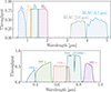 |
Fig. 1. Throughput of the filters used through this work. On the top panel we show the four Euclid filters: IE, YE, JE, and HE, along with two IRAC filters at 3.6 μm and 4.5 μm. In the bottom panel, we include the four UNIONS filters that will complement the Euclid data in the northern sky: CFIS u and r, HSC g and z, and PAN-STARRS i. |
The EDF has already been observed with the Spitzer Space Telescope’s Infrared Array Camera (IRAC, Werner et al. 2004; Fazio et al. 2004) at 3.6 μm and 4.5 μm. These observations are described in detail in Euclid Collaboration (2022a, 2024e). When dealing with the EDF, we also include these two photometric filters, assuming the same observation depth reported in Euclid Collaboration (2024e).
For convenience, the full set of filters is also listed in Table 1, with the corresponding expected 10σ observation depths for a generic extended source (in a 2″ aperture, i.e., a typical Euclid extended source) per band in the EWS – with attached IRAC observed depths in the same aperture for the EDF.
Set of filters used in this work.
2.2. The Euclid simulated fields
We simulate different versions of Euclid observations by adding realistic photometric noise to each band depending on the number of reference observation sequences that are going to be observed (ROS, see Fig. 8 of Euclid Collaboration 2024h) and the expected limiting magnitudes of the survey. A galaxy is kept in the catalog if it is detected either in HE at S/N > 5 or in IE at S/N > 10, given the expected limiting magnitude. Those limits were used because they enable a posteriori selections for other Euclid analyses, such as cluster detection and weak lensing analysis.
The four simulated catalogs (see Table 2 and Fig. 2) are:
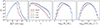 |
Fig. 2. Four simulated Euclid catalogs used in this work (solid purple line, EWS; dashed orange line, C16; solid gray line, C25; dashed-dotted blue line, EDF) shown as the number of sources as a function of the EuclidHE band magnitude (leftmost panel), redshift (center left), stellar mass (center right), and star formation rate (rightmost panel). We notice that the magnitude cut upon which the fields are built is an OR condition on the S/N in HE, IE filters; as such, simulated galaxies are found below the nominal limiting magnitude cut for HE band, as those are detected at S/N > 10 in IE. |
-
Wide, a single ROS at limiting magnitudes of HE, lim = 23.5 and IE, lim = 25.0, simulating what is expected from the EWS (Euclid Collaboration 2024h).
-
C16, 16 ROS at limiting magnitudes of HE, lim = 25.0 and IE, lim = 26.5, corresponding to a limit 1.5 mags deeper than the EWS. This simulates the so-called Euclid auxiliary fields (Euclid Collaboration 2024h), six well-known regions with vast ancillary information, observed for photometric and color calibration; 16 ROS are expected to be observed by the time of DR1.
-
C25, 25 ROS at limiting magnitudes of HE, lim = 25.25 and IE, lim = 26.75, corresponding to a limit of 1.75 mags deeper than EWS. This simulates the expected final average number of ROS to the Euclid auxiliary fields.
-
Deep, 40 ROS reaching limiting magnitudes of HE, lim = 25.5 and IE, lim = 27.0, corresponding to an expected limiting magnitude of 2 mags deeper than EWS, simulating the minimum number of ROS of the different fields composing the EDF (north, south, and Fornax).
Four simulated Euclid catalogs.
We notice that the magnitude limits reported here are different from the ones in Euclid Collaboration (2024h), which refer to point-sources at 5σ. Here instead, we convert those to 10σ limits for an extended source with a 2″ aperture (as a proxy for a typical Euclid extended source).
We are building the calibration fields by improving the EWS photometry on the Euclid and UNIONS filters; however, the real auxiliary fields, such as the Cosmic Evolution Survey field (COSMOS; Scoville et al. 2007) will benefit from a wealth of multiwavelength ancillary data (i.e., the COSMOS2020 catalog, Weaver et al. 2022) that will yield better photometric redshifts and physical parameter estimation with respect to what we report in this work.
There are a few caveats about the simulated catalogs. While the photometric noise for all the considered mock catalogs is simulated in the most realistic way possible, we are still dealing with an idealized situation where the photometric procedures are bypassed. Moreover, within the catalogs, we are considering galaxies only, without accounting for any source of contamination that the real Euclid data will have to deal with: contaminants such as stars, photometric masks (e.g., from stars) and defects (snowballs, cosmic rays, persistence from solar flares), AGN and QSOs (López-López et al. 2024), under-deblended and over-deblended objects, Local Universe extended objects, and low surface brightness galaxies. While all of those are expected to be reduced to the minimum possible (i.e., by exploiting ML to automatically classify stars and galaxies, see e.g. Cunha & Humphrey 2022, whose reported F1-scores are ∼98%), some degree of performance degradation will be unavoidable.
Finally, as the absolute best-case scenario, yielding the best possible value for each quality metric, we report the results coming from the unperturbed version of the survey, that is, the MAMBO generated catalog without any photometric noise added, run on the ground-truth magnitudes. Regardless of the flaws that may be inherent in the simulations, whatever uncertainty is generated from this set of photometric values and parameters depends only on the technique used to derive the second from the first, such as badly interpolated holes in the feature space for ML algorithms or a lack of SED models and degeneracies between colors and physical properties for template-fitting algorithms.
3. Methodology
In this section, we describe the algorithms and metrics used to assess the model’s performance in recovering the ground truth. In particular, we focus on the recovery of photometric redshifts z and two physical parameters: stellar masses log10(M⋆/M⊙) and star formation rates log10 (SFR/M⊙ yr−1), and the relation between them, the star-forming main-sequence (SFMS).
3.1. Feature, labels, and samples
In line with the standard ML terminology, we now designate the catalogs’ photometry and subproducts (i.e., broad-band photometry and colors) as features, and the model output (i.e., redshifts and physical properties) as labels. In this work, we address two versions of the latter:
-
the true labels, which are the ground-truth z and physical properties extracted from MAMBO;
-
the recovered labels, whose values have been obtained by running a traditional template-fitting code (Phosphoros, see Sect. 3.3) on the (simulated) Euclid observed features.
Thus, we can check what the best possible performance for a particular run is (i.e., when the redshifts and physical parameters are perfectly known) to compare with the more realistic ones that will be obtained with Euclid data, when the ground truth will be inevitably unknown and recovered labels will be built from the observed features as the model input samples. This information is useful, especially in cases where the EWS performance are evaluated with a reference sample built from the calibration fields (see in the next paragraphs). As reported in Sect. 2.2, the simulated ones have labels recovered from the same set of filters as the EWS, but the real ones will benefit from lots more multiwavelength data, with better recovered photo-z and PPs. The expected real performance of such cases should therefore be in between the recovered and true labels performance.
Every supervised ML application is composed of a training (or reference2) sample from which the relations between features and labels are inferred, and a target (or test3) sample on which the models are applied. As described in Sect. 2, we have four different simulated versions of Euclid observations, mimicking the expected outcome of the EWS, EDF, and two calibration (auxiliary) fields. As common practice in ML applications, we split those catalogs, using part of the sample for training (or as references) and the rest equally split for cross-validation and testing. In this work, we used 90% of the samples for training (translating into training sets between 500 k and one million galaxies), ensuring at least ∼50 k galaxies in the test sample, which is more than enough to evaluate the model’s performance.
To understand the actual performance expected from the observed Euclid data, we explore the predictive capabilities of models trained on deeper photometry when applied to a shallower one (in this case, the EWS). For instance, this is achieved by training a model using the EDF catalog and subsequently evaluating it on the EWS catalog. In those cases, at test time, we share the same set of train and test sources between the catalogs to be as consistent as possible. The same is done for every ML method used in this work, and we share the same train, reference, and test samples for the same catalog permutation between different models (e.g., when testing the performance of a model trained on the EDF catalog and tested on the EWS one, the training and test source IDs are the same for all the methods considered).
When dealing with recovered labels, in order to simulate a typical application where the ground truth is unknown as Euclid will observe photometry from which the photo-zs and physical parameters will be derived, we train the models on those and test on the true labels.
3.2. Features engineering
As reported in Sect. 2, in standard ML terminology, the catalogs observed photometric values are the features of the models. At the base level, each entry in the features space is a single galaxy’s simulated photometry, in magnitudes; that is, the nine Euclid + UNIONS bands for the EWS, with the addition of two IRAC bands for the EDF. In order to improve the quality of the models, thus the model inferences, we also include derived features as the colors (pairwise differences of the magnitudes, excluding permutations), increasing the number of total features to 45 (EWS) and 66 (EDF). This is the number of features for each of the previously described methods, with the notable exception of the CatBoost chained regressors (CCR), where the inferred labels are added on top of those as new training features at each iteration, as described in Sect. 3.5.2.
All of the methods presented in this section are not sensitive to the dynamic range and scales of the input features, except for the Deep Learning Neural Network (DLNN). In that case, we scale the features to a similar dynamic range with a standard Z-score normalization.
3.3. Phosphoros
Phosphoros4 (Paltani et al., in prep.) is a Bayesian template-fitting tool for galaxies SED developed within the Euclid collaboration. In the Euclid photo-z data challenge, which evaluated the performance metrics of different template-fitting and ML codes in retrieving the photometric redshift of a mock catalog, Phosphoros yielded the best performance along with LePhare (Euclid Collaboration 2020).
Phosphoros can be used to evaluate at the same time the photometric redshift and the physical properties of galaxies that have to be provided as tags for the templates. In the present work, we have used 1254 templates from Bruzual & Charlot (2003, in the 2016 version5) with Chabrier IMF (Chabrier 2003), considering exponentially declining (e-folding timescale τ = 0.1, 0.3, 1, 2, 3, 5, 10, 15, 30 Gyr) and delayed (characteristic timescale τ = 1, 3 Gyr) star formation histories, 2 metallicities (Z = 0.008, 0.02) and 57 ages between 0.01 and 13.5 Gyr. The internal dust attenuation has been modeled with Calzetti’s law (Calzetti et al. 2000) with E(B − V) values in the range [0.0, 0.5]. We tested whether the IMF choice for the templates might bias the performance by running Phosphoros with templates built with Salpeter IMF (Salpeter 1955), finding identical results in terms of performance metrics (see Sect. 3.6), though almost monolithically shifted by a factor 0.23 dex in logarithm with respect to the Chabrier results, shown throughout the paper.
As a first step, a grid with model photometry is derived for all the templates in the redshift range z ∈ [0.0, 6.0] with steps of dz = 0.01. When comparing the model to the observed photometry, the only factor considered prior is the “volume-prior”, proportional to the redshift-dependent differential comoving volume. Upper limits are treated in a statistical sense, as models with fluxes over the limit in the undetected bands are still considered when looking for the best-fit model; in those cases, the χ2 evaluation follows the indications in Sawicki (2012). In the version that will be used for Euclid data, there will also be the possibility of consistently dereddening the photometry for the Galactic extinction (Galametz et al. 2017) and considering the variability of the filter transmission functions across the field of view (Euclid Collaboration 2024g). A recipe to add emission lines is also implemented in Phosphoros, but not used in this work.
The final result of the computation is the characterization of the multidimensional posterior with a density sampling of 100 values for each galaxy, as well as the values of the physical properties and redshift from the best posterior model as the mean, the median (used in this work), or the mode of the distribution.
In this work, we use Phosphoros results to benchmark ML methods against a standard template-fitting algorithm and as a necessary step to build the reference sample to use as input for nnpz.
3.4. nnpz
The Nearest-Neighbors Photometric Redshift (nnpz, see Tanaka et al. 2018, for a first application on the HSC-SSP survey) is a supervised-learning technique mapping a given set of features to known labels with an upgraded version of the k-nearest neighbors algorithm (k-NN). In its most simple form, a k-NN algorithm combines an integer number of k neighbors in a reference sample closest to the target in feature space with respect to some distance metric (e.g., Euclidean) and predicts a label based on some user-defined combination of the metrics of the k-NN reference sample labels (e.g., a mean weighted by the distance in feature space). The same conceptual approach can be employed to provide a posterior distribution function (PDF) for the desired label by combining some a priori known PDFs for the reference sample under the assumption that similar observations with similar uncertainties would naturally produce similar results. Predictions and confidence intervals will naturally follow from the output PDF.
This is the concept behind nnpz in a nutshell. The reference sample is built starting from Phosphoros as a set of objects whose full parameters’ PDF has been sampled with 100 randomly extracted points according to the PDF density distribution. The samples of the k-NNs are then combined to produce the target PDF, from which a punctual prediction is obtained from the mean, the median, or the mode of the distribution.
In this work, we used the 1.2.2 version of nnpz available on the EuclidLOcal DEvelopment ENvironment (LODEEN) version 3.1.0, a virtual machine containing all of the Euclid software and pipelines. As for the code hyperparameters, after a first skim in a batch of at least 1000 nearest neighbors in the target space obtained from a space partition with KDTree (necessary to speed up the whole process instead of simply brute-forcing the search), we fix the final k from which the target labels are evaluated to 30 nearest neighbors. To generate a prediction, each neighbor is weighted with its χ2 likelihood, which is the χ2 distance between the reference neighbor and the target point in the feature space. nnpz combines the posterior coming from all the nearest neighbors and produces a PDF for the predicted target galaxy, from which we extract the point prediction as the median value of the distribution. We perform the same tests presented in this work with the mode of the distribution (i.e., the maximum-likelihood estimator) as the point prediction without noticing a significant change in the results.
In fact, returning a source’s multivariate PDF samples as output instead of a single-point prediction is one of the great advantages of nnpz. This information is in principle recoverable with other ML algorithms, such as CatBoost (see Mucesh et al. 2021, for an application to a simple random forest) if considering all the training samples in a particular leaf as PDF samples, though this is computationally and memory-wise less feasible than the ∼100 samples per galaxy of nnpz.
3.5. Other machine learning techniques
Apart from nnpz, we performed similar tests using previously tested ML techniques that have been shown to be extremely efficient for redshift and galaxy property estimation: Gradient-Boosted Decision-Trees (GBDT) and DLNN.
3.5.1. CatBoost single-model regressor
A GBDT is rooted in decision trees, a building block of widely used and successful techniques for regression and classification tasks. In a decision tree, the data is recursively split into smaller subsets based on the features that best separate the data according to some information gain (for classification) or variance minimization (for regression) criteria, until a stopping criterion is met. The result is a tree-like structure, with each internal node representing a feature, each branch representing a potential value for that feature, and each final node (leaf) representing a class (for classification) or predicted value (for regression). This scheme has been improved by what is called gradient boosting, which decreases the randomness improvement in training by starting with a set of imprecise decision trees (“weak learners”) and iteratively improving them, focusing on what these are predicting wrong rather than generating a new random subset of the data.
CatBoost (Prokhorenkova et al. 2018)6 is a cutting-edge ML algorithm specifically designed for gradient boosting on decision trees. There are some specific features that help reduce some typical issues in gradient boosting algorithm implementations, such as the ordered boosting to reduce overfitting and the oblivious trees to regularize while increasing speed.
In this work, we use CatBoost in two different ways. With the CatBoost single-model regressor (CSMR), we train a single model to solve a multiregression problem. Each set of features is associated with a pool of labels (zphot, M⋆, SFR) and not just a single label per time (as in Sect. 3.5.2), finding the best model with a Multivariate Root Mean Square Error (MultiRMSE) loss. In each case presented, the final model is trained with 1000 estimators, allowing for a maximum depth of 11.
3.5.2. CatBoost chained regressors
With the CCR we train on a set of features one label per time, and iteratively append the predicted labels to the features up until convergence, allowing the model to naturally learn the correlation between parameters through an iterative approach. A thorough and more detailed description can be found in Humphrey et al. (in prep.). Here, we summarize it in the following paragraph.
We start with a training set (Xtrain, ytrain) and a test set (Xtest, ytest). The first iteration goes as follows:
-
The model is trained on Xtrain whose features are the full set of colors and magnitudes (with permutations, see in Sect. 3.2), with only zphot as the lone label in ytrain. From this model, we can predict some zphot and evaluate their performance metrics on the test sample.
-
Now, the model is trained on a new Xtrain that is composed of the previous ones (magnitudes and colors) and the zphot predicted in 1. From this model, we predict log10(M⋆/M⊙) and evaluate the log10(M⋆/M⊙) performance metrics on the test sample; of course, the Xtest has been extended to incorporate the new feature from the predicted zphot on the test sample.
-
Then, the model is trained on another Xtrain composed of the previous features plus the predicted log10(M⋆/M⊙) in the previous step. With this model, we predict log10 (SFR/M⊙ yr−1) and evaluate the log10 (SFR/M⊙ yr−1) performance metrics on the (once again, extended) test sample.
Now the second iteration starts.
-
The model is trained on an Xtrain composed of the previous features – including the zphot and log10(M⋆/M⊙) predicted in steps (1) and (2) – plus the predicted SFRs in step (3), and with this model, we re-predict zphot and evaluate their performance metrics.
-
Again, another model is retrained with the previous features plus the new zphot predicted in the previous step. log10(M⋆/M⊙) is re-predicted, and the model performance on the label is evaluated.
The whole procedure goes on for four iterations, when we observe a convergence of the evaluated metrics in agreement with Humphrey et al. (in prep.).
As such, the model features are (in square brackets, the step in which they have been evaluated):
-
magnitudes and colors;
-
magnitudes, colors, and zphot;
-
magnitudes, colors, zphot, and log10(M⋆/M⊙);
-
magnitudes, colors, zphot, log10(M⋆/M⊙), and log10 (SFR/M⊙ yr−1);
-
magnitudes, colors, zphot, log10(M⋆/M⊙), log10 (SFR/M⊙ yr−1), and zphot.
And so on, for four iterations.
Finally, we store the final set of label predictions for the test set on which we evaluate the performance metrics (see Sect. 3.6). In running CatBoost we use the same set of hyperparameters as in CSMR and in Humphrey et al. (in prep.).
3.5.3. Deep learning neural network
As we only deal with structured (i.e., tabular) data, we also test the performance of a simple, multilayered DLNN. Here we adopt a typical architecture that has been widely used in the literature in searching for photometric redshifts and physical parameters (e.g. Firth et al. 2003; Collister & Lahav 2004; Euclid Collaboration 2023).
The DLNN inputs are the training features (magnitudes and colors, with permutations, see Sect. 3.2), and the output is a set of three labels (zphot, M⋆, SFR). The DLNN architecture (described in Table 3) consists of five fully connected layers with a decreasing power of two hidden units for each layer. The adopted activation function for each layer is a Rectified Linear Unit (ReLU, Nair & Hinton 2010), Mean Squared Error (MSE) for the loss function with L2 regularization to avoid overfitting, and the model is optimized with the ADaptive Moment estimator (Adam, Kingma & Ba 2014).
Architecture of the DLNN used in this work.
The DLNN for each model are trained and tested on the same train and test samples as for all the other methods. We run the training on mini-batches of size 512.
3.6. Metrics and quality assessment
We use standard metrics to quantify the model’s performance. Those are defined differently when referring to redshifts or PPs.
The first is the normalized median absolute deviation, defined as:
 (1)
(1)
with b being the model bias (see below).
The outlier fraction fout is defined as the fraction of catastrophic outliers (Hildebrandt et al. 2010) over a certain threshold (in log space for physical parameters, linear for redshifts):
 (2)
(2)
These thresholds have been evaluated looking at the standard deviation of the PPs distribution, considering only sources with a good photo-z recovery – that is, below the 0.15(1 + z) threshold – for all the methods considered, trained with true labels (see Sect. 3.1). As a consequence, the PPs thresholds are not the same for stellar masses or SFRs. The chosen thresholds are two times the mean standard deviation between the prediction and the true values found for all the considered methods, rounded to the nearest decimal. The values are tout = 0.4 dex for stellar masses and tout = 0.8 dex for SFRs.
Defining the catastrophic outliers in this way is different than assuming a plain 0.3 dex difference between the prediction and the true values of the physical parameters (corresponding to a factor of two) that is found in recent literature (e.g. Euclid Collaboration 2023). Fixing the same value in dex space for every PP is a penalizing choice, especially for SFRs, where a 0.3 dex difference might even be the order of (or even below) 1σ of the distribution, which is too little to define a galaxy as a catastrophic outlier. In this way, we adopt a more robust definition from a statistical sense, which actually returns an informative quantitative description of what a catastrophic outlier is for a stellar mass estimate or a star formation rate.
Finally, a model’s overall bias b is:
 (3)
(3)
In all three cases, the closer to zero, the better the predicted values resemble the test ones. Of all three, only the bias can take either positive or negative values.
We notice that those metrics are different from the Euclid requirements, that depend on the redshift probability distribution functions (PDZ, see their definition in Sect. 4.2 of Euclid Collaboration 2020). We use photo-z and PPs point estimates instead.
As for the SFMS, we evaluate the performance of the recovered relation by evaluating three parameters:
-
the relation slope m, measured with an orthogonal distance regression (ODR);
-
the fraction of passive galaxies fp, defined as the fraction of objects with specific-SFR
 . This limit has been determined looking at the divide between passive and nonpassive galaxies in MAMBO and is in accordance with values found in the literature (e.g. Pozzetti et al. 2010; Ilbert et al. 2013);
 -
the relation scatter σ, measured only on nonpassive sources.
4. Results
In this section, we present the results of the methods presented in Sect. 3 on the simulated Euclid fields described in Sect. 2. Our primary objective is to evaluate the performance of the methods described in Sect. 3 and find the optimal strategies to extract the maximum amount of information available in the Euclid survey, in particular the EWS and EDF. We ought to do so by dealing with realistic information, that is, what the survey will actually deliver as a scientific product. As such, we present results for the EWS and for the EDF, obtained by combining the Phosphoros results (photometric redshifts, physical parameters) in the fields with the available photometry. As described in Sect. 2, we deal with two kinds of training labels: the true ones (i.e., the ground-truth simulated parameters), which of course are unknown in a real-life application, and as such, we only use them to assess what the best-case scenario for a particular field could be, and the recovered labels, whose values are the Phosphoros outputs resulting from the observed photometry, which is what an actual application to real Euclid data will have to deal with. However, it is worth noticing that spectroscopic redshifts will be available for a smaller sample (still around the order of millions of sources), which is the closest thing to true labels that the EWS and EDF will yield. A similar argument (with lots of attached caveats) could apply to those sources with Hα-derived SFRs, though the numbers in this case are sensibly reduced with respect to the spectroscopic redshifts. For each trained model, we carefully checked that the performance metrics evaluated on the training set do not differ significantly from the ones obtained by applying the model to the test set, thus excluding any kind of overfitting to the training set.
4.1. Computational performance
Most of the runs presented here – specifically, the CSMR, CCR and DLNN results – are performed on Galileo100, a high-performance computing (HPC) system located at Cineca, within the Italian SuperComputing Resource Allocation (ISCRA7) Class C program, as part of the PPRESCIA-HP10CBAZOH program (PI, Enia). Galileo1008 is a DUal-Socket Dell PowerEdge cluster, hosting 636 computing nodes each with two x86 Intel(R) Xeon(R) Platinum 8276-8276L, with 24 cores each. In fact, the main advantage of ML methods over classic template-fitting templates is the dramatic speed-up to the inference problem, at least when dealing with point value prediction for the parameters, coupled with the improved computational performance in training these models in HPC systems.
Phosphoros and nnpz are run on a PowerEdge T640 machine with an Intel(R) Xeon(R) Silver 4116 CPU @ 2.10 GHz processor, and 24 available cores. A typical run of Phosphoros requires ∼0.8 seconds per galaxy; for a number of galaxies around a million (as in our cases), it translates into uninterrupted runs of a couple of weeks on the 24 available cores of our workstation.
With nnpz, which technically does not need training as the whole computational load is on the shoulders of the neighbor search and PDF combination, a typical run on a target sample of ∼50 k galaxies requires ∼8 minutes of time, or 0.006 seconds per galaxy, a speed-up of a factor 100 with respect to Phosphoros.
CatBoost-based runs and DLNN require training instead, after which the inference is almost instantaneous. How long those methods will run depends on the size of the training set, how complex the model is allowed to be and the number of training epochs for DLNN; for a typical training set size of a million galaxies, it translates into training runs of ∼15 minutes for CSMR on 16 cores, ∼0.002 seconds of training time per galaxy. For CCR the training time per galaxy is similar, though the final run is of course longer since a model is trained at every iteration for each label. We run the CCR on Galileo100, asking for a single node of 48 cores, whose overall run lasted for ∼1 hour time.
Finally, on the same HPC system, we trained the DLNN for 300 epochs, translating into ∼7 hours of training time (∼80 seconds per epoch) for a ∼ million galaxies in the training sample, a training time of ∼0.003 seconds per galaxy.
4.2. Phosphoros results
The first results we present are the template-fitting runs with Phosphoros on all the galaxies present in the training (or reference) samples. We refer the reader to Sect. 3.3 for further details on how Phosphoros has been run. The results are shown in Fig. 3, for the simulated EWS and EDF. In Appendix B we also show the results for the two auxiliary fields at 16 and 25 ROS. In each plot, the true values are plotted against the recovered ones, and the performance metrics are reported in the bottom right of each plot.
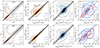 |
Fig. 3. Phosphoros results on two simulated Euclid catalogs, EWS (top panels) and EDF (bottom panels), with true values plotted against the Phosphoros recovered ones. The black line is the 1:1 relation; the shaded area is the region beyond which a prediction is an outlier. In every plot, the four contours are the area containing 98%, 86%, 39% (corresponding to the 3σ, 2σ and 1σ levels for a 2D histogram) and 20% of the sample. For SFMS the true distribution is reported in red (dashed), the predicted one in blue (solid). The lines are the ODR best-fit to the (passive-removed) distribution. The reported metrics are NMAD (purple), the outlier fraction fout (blue) and the bias (green) for the photometric redshifts and physical parameters, and the slope m, scatter σ and fraction of passive galaxies fp for the SFMS, all defined in Sect. 3.6. |
These results are sort of the blueprint for all the others found in this work. The first thing that jumps out is the difficulty in recovering the correct SFR, as both the EWS and EDF simulations display high NMADs (0.90–0.77, respectively) and fractions of outliers (> 30%). The recovered SFRs for the EWS are also biased toward higher values by a factor ∼1.4 (a bias of 0.13–0.15 in the logarithm).
Optimal recovery is obtained for photometric redshifts instead, with NMADs that improve from 0.057 to 0.035 passing from Wide to Deep photometry – and the addition of the two IRAC bands – and fout reducing from 22% to 10%, with half of this reduction the consequence of an improvement in correctly distinguishing faint low-z, low-mass objects from high-z, high-mass ones. For the EWS, worse results are obtained for the stellar masses, with higher NMADs (0.258) and fractions of outliers (22%). The combined effect of deeper photometry plus the two IRAC bands sensibly improve the recovered stellar masses in the EDF, with NMADS decreasing to 0.18 and fout to 11%. Both the recovered photometric redshifts and stellar masses show low biases (absolute values smaller than 0.04) with respect to the ones found in the SFRs.
These are not unexpected findings, given the specific set of filters used as input. As reported in Sect. 2 (see also Table 1 and Fig. 1), for the EWS we use 9 filters with rest-frame λeff between 0.37 μm and 1.77 μm. As the photometric redshifts are more sensitive to colors in the ultraviolet (UV)-to-NIR part of the spectrum, these are well recovered with the given wavelength range and the number of filters. Moreover, dropouts in different filters are an excellent proxy for high-z galaxies. Stellar masses correlate well with rest-frame NIR photometry, in particular the HE band, and most of our simulated sample (> 60%) reside between 0 < z < 1.5 where NIR is still sampled by Euclid filters. The addition of the first two IRAC channels helps significantly in improving the stellar masses recovery. Things are harder for SFRs, as they correlate the most with mid-IR to far-IR photometry (Kennicutt & Evans 2012), tracing obscured star formation, and secondly with UV rest-frame monochromatic fluxes at 1550 Å (FUV, Bell & Kennicutt 2001) and 2800 Å (NUV, Bell et al. 2005), tracing unobscured star formation. The former, stronger proxy is inaccessible with the chosen set of filters, while the latter is a weaker one. This makes the recovery of SFRs difficult even in an ideal, pristine situation (see Sect. 4.3 and Table 4) and extremely complicated when more sources of uncertainty are added. These could be improved by imposing some SFR-related priors to the template-fitting algorithm, something that will be carefully considered when dealing with real Euclid data.
Metrics for the unperturbed simulation.
The main fraction of photo-z catastrophic outliers (around 10% for the EWS, 5% for the EDF) is composed of faint low-redshift (ztrue < 1), low-mass [log10(M⋆true/M⊙) < 9] and low-SFR galaxies [ ] that are instead misplaced at higher redshifts (z > 2) with at least one order of magnitude higher masses [log10(M⋆/M⊙) > 10] and SFRs [log10 (SFR/M⊙ yr−1) > 1]. This is reflected in the SFMS. In the EWS case, the higher SFR overestimation with respect to stellar masses yields a fitted relation with a sensibly higher slope (m = 2.1) with respect to the true one (m = 1.3). The uncertainties on the recovered parameters translate also into a higher scatter of σ = 0.48 (ground truth of 0.30) and a fraction of passive galaxies higher (fp = 12% instead of 6%). Things get better for the EDF, with metrics still distant from the true ones though.
4.3. The unperturbed simulation
One might wonder what the absolute best-case scenario is in terms of performance when applying the methods described in Sect. 3 to a pristine, unperturbed set of features mapping to the true labels. This is the same as asking what order of magnitude the irremovable inherent uncertainty of those methods is, which will always affect the measured metrics, even in a more realistic scenario where the noise affecting the features (and labels) will dominate.
To answer this question, we run the methods defined in Sect. 3 on an unperturbed, noise-free features version of the MAMBO catalog with true labels (see Sect. 2 for definitions). Any uncertainty depends only on the specifics of the technique used to map features to labels and, from a broader perspective, on how well those specific features (magnitudes and colors) are able to recover those particular labels (photometric redshifts, stellar masses, and star formation rates).
The results are reported in Table 4. What stands out is the perfect recovery of the photometric redshifts, up to a 0.1% fraction of outliers. Those nine filters and the associated colors are able to correctly put a galaxy in its right place in the cosmic picture (see Appendix A for a quantification on the feature importance). This is similar for stellar masses, though with metrics degraded by an order of magnitude, NMADs of ∼10−2 vs ∼10−3 for photo-zs – and comparable outlier fractions – as expected once considering that the rest-frame H band is a well-known tracer for correctly identifying the galaxy mass content, which is still true as the majority of the simulated sources are at z < 1.5.
Star formation rates are harder to recover, though. Even in an ideal, perfect scenario, it is impossible to go below NMADs of ∼0.13 for that particular set of features. Of course, there is room for improvement if adding other features more sensitive to the star formation processes when available, for instance, mid-IR or far-IR photometry, or spectral features, such as the Hα emission line. A more detailed dissertation is beyond the scope of this work, which focuses mainly on the EWS and EDF, without considering other ancillary (or new) filters. However, the complete exploitation of the full spectrophotometric (and morphologic) information in Euclid will be explored in a forthcoming work.
4.4. Results for the Euclid Wide Survey
The unperturbed case gives back an extremely optimistic best-case scenario. In reality, all the observed photometry in Euclid will be affected by some degree of uncertainty, whose effect is to make the feature space noisier, mixing together sources with different labels. At times, even with extremely different ones, in degenerate regions of the feature space (i.e., fainter and less massive or brighter and more massive), making it hard – or even impossible – to correctly understand which label is associated with that particular set of features. This unavoidably degrades the quality of the model and the performance metrics when applied to a sizable sample of data.
As reported in Sect. 2, we simulate four different versions of Euclid observed catalogs: the EWS and EDF, and two calibration fields with 16 and 25 ROS, respectively, mimicking the Euclid auxiliary fields for photometric and color gradient calibration (Euclid Collaboration 2024h). In this section, we focus on the EWS, and the performance observed when training the models on deeper samples.
We present two possible approaches for this task. In the flowchart shown in Fig. 4, we summarize what has been done in obtaining the reported results for the EWS (top panel) and the EDF (bottom panel). The flowchart describes the different approaches employed when dealing with simulations at different depths of the same field.
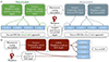 |
Fig. 4. Flowchart followed for the reported results on the EWS and EDF. Panel (a) summarizes what has been done for the EWS. In this case, we employed two different approaches: pairing features to labels coming from Phosphoros results at the corresponding depth (paired labels), or with features always from the Wide simulated catalog and labels coming from Phosphoros results at the Calibration and Deep fields depth for the corresponding sources (mixed labels). These pairs of (features, labels) – or (features, posteriors for nnpz (see Sect. 3.4) – are thus given as input for the ML models described in Sect. 3. Panel (b) illustrates the straighter flowchart for the EDF, where the pairs (features, labels) or (features, posteriors) always come from the simulated Deep field. |
4.4.1. Paired labels approach
The first one is the paired labels approach. Here, we train each model (or build a reference sample) with features and labels coming both from a particular field (EWS, EDF, or the two calibration fields), and test on the EWS. The labels are the recovered ones (see Sect. 3.1), that is, the Phosphoros results for photo-z and physical parameters on the field-correspondent photometry. The results are summarized in Table C.1, where for each pair of training/reference – test field we report the performance metrics for all the considered labels, and Table C.2, where we report the same for the SFMS results.
The photometric redshifts performance is good, in line with the template-fitting results in Sect. 4.2 (see top panels of Fig. 5). There is a slight improvement in training the model with photometry and labels coming from deeper fields, with NMADs reducing by ∼0.01 and outliers by ∼5% at best. nnpz has the best results overall (NMAD ∼ 0.06, fout ∼ 18%), for every possible case of training field involved. The vast majority of outliers – raising the NMAD too – are z < 1.5 galaxies mistakenly assumed to be higher redshift ones at z > 2 (more on that in the next paragraphs). When looking at their magnitudes, these objects are revealed to be faint galaxies, with a distribution peaking close to the magnitude limits for each band.
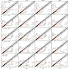 |
Fig. 5. Results for the EWS with the mixed labels approach. The true values on the x-axis are plotted against the predicted values on y. The black line is the 1:1 relation; the shaded area is the region beyond which a prediction is an outlier. Contours are the area containing 98%, 86%, 39% (corresponding to the 3σ, 2σ and 1σ levels for a 2D histogram) and 20% of the sample. Each column represents the results for the methods described in Sect. 3. In the first four rows, the training labels are the recovered ones, coming from Phosphoros results to the mock photometry at the same depth of the field reported in the leftmost plot legend and tested on the EWS (see Sect. 2 for further details). The T.lab Wide-Wide case is exactly the same as the Wide-Wide case in Table C.1. In the fifth row, we show the results of the EWS training the models with their true labels as the best-case scenario for that particular field. The reported metrics are NMAD (purple), the outlier fraction fout (blue) and the bias (green) for the photometric redshifts and physical parameters, as well as the slope m, scatter σ and fraction of passive galaxies fp for the SFMS, all defined in Sect. 3.6). |
This wrong distance attribution is carried over to the stellar mass prediction. A part of the degradation in the NMAD and most of the one in fout is a consequence of those lower-z, lower-mass galaxies mistakenly assumed to be as high-z, high-mass ones. At best, with the given features and true labels in the training sample, no less than NMAD ∼ 0.14 and fout ∼ 13% is expected (with the CCR, see bottom panel of Fig. 6). For stellar masses, no improvement is observed when using deeper calibration fields for training but rather a degradation (see Table C.1, with the exception of EDF field, with the two IRAC channels). This is not unexpected, as it is common in ML applications to see cases where training and testing on noisier data altogether yields better results than training with better features and testing on the noisy ones.
The most worrisome metrics are the ones associated with SFRs. The outlier fraction, defined as points with predicted SFR above or below a certain threshold to the true value (0.8 difference in log space, Sect. 3.6), is over 30% for every method with the notable exception of nnpz, where it stays between 26% and 30%. We already showed in Sect. 4.3 how recovering SFR with the given set of features is harder than photo-zs or stellar masses even in the ideal, unperturbed case. In a more realistic scenario, the results of the EWS are far from ideal, even when the true values for SFR are used in the training process (no less than an NMAD of 0.38 and 10% of outliers, see bottom panel of Fig. 7). The template-fitting algorithm finds it hard to recover SFR indeed, as reported in Sect. 4.2 (∼39%). Differently than stellar masses, this is not just a matter of the wrong photo-zs attribution affecting the SFRs (i.e., closer and less star-forming vs farther and more star-forming; more on that in the following paragraphs), but an inherent degeneracy due to the filters and colors used in the inference process.
The occurrence of simultaneous wrong predictions for stellar masses and SFRs (both overestimated or underestimated) mitigates the impact on the recovered SFMS, at least regarding the relation slope m, when training with deeper photometry (Table C.2). However, with the notable exception of nnpz, which yields the best performance in terms of SFRs, the recovered fraction of passive galaxies [ ] is usually well overestimated by a factor of two, the true one being 6%. No method at whatever training depth is able to recover the correct relation scatter (σ = 0.24).
4.4.2. Mixed labels approach
Trying to mitigate the effect of the aforementioned cloud of catastrophic outliers, we tried another approach, rooted in the belief that better performance should arise in training the models with the best possible set of labels for a given set of features. We refer to this one as the mixed labels approach, whose results are reported in Figs. 5–8 and Tables 5–6.
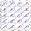 |
Fig. 8. Same as in Fig. 5, but for the SFMS. Dashed red contours are the test SFMS (i.e., the true values), solid blue is the predicted one. Contour levels are the same as reported in Fig. 5. The lines are the ODR best-fit to the passive-removed distribution (dashed for test SFMS, solid for predicted). The reported metrics are the SFMS slope, scatter, and fraction of passive galaxies, defined in Sect. 3.6. |
Metrics for the EWS, with the mixed labels approach.
Metrics for the recovered SFMS in the EWS, with the mixed labels approach.
Differently from the previous approach, here we train the models with features (magnitudes and colors) always coming from the EWS catalog. However, for the deeper fields, the training labels are the Phosphoros results obtained with the corresponding photometry. This is specified in the plot with the text Training Label (T.lab.) followed by the name of the field. The model is then tested on features and (true) labels of the EWS.
To give an example, when referring to T.lab Deep - Wide we mean:
-
training features from the EWS;
-
training labels from the Phosphoros results obtained with the Euclid Deep photometry;
-
test with features from the EWS and as labels the true values for zphot, log10(M⋆/M⊙) and log10 (SFR/M⊙ yr−1).
The mixed labels T.lab. Wide-Wide case is exactly the same as the paired labels Wide-Wide case, so the first rows of Table C.1 report the same values as the first rows of Table 5 and shown in Figs. 5–7. Notice also that with this approach we reduce the number of galaxies in the reference/training samples, as only those detected in the EWS will have Phosphoros recovered labels, thus the number of training galaxies passes from the ∼ one million for the Deep and calibration fields to ∼500 k (in Sect. 4.4.3 we reduce it to ∼230 k to simulate a more realistic COSMOS-alike reference sample).
However, despite the reduced training set, this approach improves the overall performance when applying the models to the test sample 9. In fact, attaching labels obtained with the best possible available photometry acts similar to a prior, which is able to guide the model in better distinguishing the cases in which there are degeneracies in the feature space where two close sets of features yield drastically different solutions (and catastrophic outliers, e.g., two faint galaxies with similar features can be either low-z, low-mass or high-z, high-mass objects), an improvement that totally compensates the loss in sheer number of training examples. This behavior in feature space translates in the photo-z predictions as a vertical strip at zphot ∼ 1, which are z < 1.5 galaxies mistakenly assumed as being farther away (see upper left panel of Fig. 3 or the top row of Fig. 5), and generating a cloud of higher mass, higher SFR galaxies in their respective plots. The wrong photo-z attribution is dragged onto the stellar masses (top rows of Fig. 6), where the outliers cloud is less prominent as in the photometric redshift case but still present as a stripe of higher mass galaxies than expected. This also applies to SFRs, which are also heavily affected by the reduced predictive power of the chosen features, as previously described.
To better illustrate what was described in the previous paragraphs, in Fig. 9 we show the distribution of true vs. predicted PPs as a function of the difference between zpred and ztrue. In the true PP – predicted PP plane, zpred − ztrue is measured as the median of the values falling within each bin. We report the results obtained with nnpz on EWS (i.e., the T.lab. Wide-Wide case), but similar things are observed for all the other methods and cases considered.
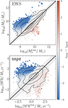 |
Fig. 9. Stellar masses (top panel) and SFRs (bottom panel), color coded with the difference between the true and predicted redshifts, for the nnpz results in the EWS trained with wide features (the upper-right plots in Figs. 6–7). Similar results are obtained for all the other methods considered. The black line is the 1:1 relation. Shaded area is the region beyond which a prediction is an outlier (0.4 dex for stellar masses, 0.8 dex for SFRs, see Sect. 3.6). Contours are the area containing 98%, 86%, 39% (corresponding to the 3σ, 2σ and 1σ levels for a 2D histogram) and 20% of the sample. The zpred − ztrue are measured as the median of the values falling in each true vs predicted bin. It is clearly visible how the wrong photo-z attribution generates the main bulk of catastrophic outliers. However, the distribution scatter along the 1:1 relation – i.e., the NMAD – is mainly due to the inherent difficulties of the methods in assigning the correct PPs given the set of input features independently from the inferred photo-z. This is particularly true for SFRs. This plot also illustrates how penalizing a 0.3 dex definition for catastrophic outliers would be with respect with the ones chosen for this work, which actually follows better the distribution of true and predicted PPs. |
Both for stellar masses (top panel) and SFRs (bottom panel), the cloud of photo-z catastrophic outliers is visible as a region of blue squares – meaning low-z objects mistakenly placed at high-z – while a minor impact is due to the opposite, in red. These regions are correctly placed outside the defined thresholds for PPs outliers (shaded area), described in Sect. 3.6, thus showing how they better relate with the distribution statistics with respect to a fixed 0.3 dex threshold. Another thing to notice is how the presence of those photo-zs outliers has a limited effect on the PPs distributions scatter (i.e., the NMADs). The majority of the distributions (> 80% of points) have |zpred − ztrue|< 0.1. Even removing all the catastrophic photo-z outliers, the NMADs would still be 0.19 (for stellar masses) and 0.58 (for SFRs). This is a consequence of the inherent difficulties of the methods (template-fitting and ML) in recovering PPs with the given set of features, that is, filters chosen to sample the galaxies emissions, even in cases where photo-z is correctly measured.
This fraction (∼9–10%) of low-z galaxies mistakenly assumed to be high-z skew the respective luminosity functions to overestimation. This is also observed in the SFMS, where the overall effect is somehow compensated by the mass-SFR scaling in the same (wrong) direction. The fit to the relation is usually way steeper than the true one when the training sample is at the same depth as the EWS, with the exception of nnpz.
With the mixed labels approach, the models will preferentially place fainter objects at lower-z with lower masses instead of the opposite. The other side of the coin is that now a fraction of truly high-z galaxies will be placed at lower redshifts. This is particularly visible with nnpz (right column of Fig. 5), and a little less with the other models. However, the net result is an improvement, as only ∼1–2% of these kinds of outliers are present in our results, while the number of low-z objects previously mistaken for high-z ones reduces by a half (from ∼10% to ∼5%).
We find that nnpz and CCR return the best performance of all the ML methods described in Sect. 3, followed by CSMR and the DLNN. In particular, nnpz returns the best results for the stellar masses and SFRs for the EWS, reducing the outlier fraction from the ∼28% of the paired labels approach to the (still high) ∼20–30% in the mixed labels one, and NMADs down to 0.61 from 0.67.
nnpz is also the best method for recovering the SFMS, as shown in Fig. 8. In the T.lab Deep – Wide case, all the methods get close to the true values, with nnpz being the closest. In fact, even in the worst case where Wide features and labels are employed in training, nnpz results are better than the ones obtained with the other methods, with a close to correct recovery of the slope and fraction of passive galaxies, despite a higher scatter (σ = 0.42 instead of σ = 0.30) and a very small parallel displacement of the relation due to an overall overestimation of the SFRs.
The whole EDF will not be finalized until the end of the mission. The EWS results will be largely inferred from the auxiliary fields. These results show that this will not significantly affect the EWS scientific outcomes, as the performance of the auxiliary fields at 16 or 25 ROS is only slightly (a few percentage points) worse than the ones with the full EDF photometry available.
We find photo-z metrics slightly outside the mission requirements (σz < 0.05, fout < 10%) As reported in Sect. 3.6, the metrics reported here are the ones measured on point predictions, while the requirements in Euclid Collaboration (2020) depend on the PDZ. Moreover, the calibration fields used here have recovered labels from applying Phosphoros to the 9 bands described in Sect. 2, while the real calibration fields will benefit from more multiwavelength observations. The net effect will be more reliable labels for training and, thus, improved metrics. While our findings lie just outside the mission requirements for photo-z, we can likely assume that real ones will meet them.
4.4.3. A COSMOS-like reference sample
The photometric and color gradient calibration in Euclid will be performed observing six of the most observed fields in the sky (the so-called Euclid auxiliary fields; see Sect. 6.2 in Euclid Collaboration 2024h, for further details). The COSMOS field (Scoville et al. 2007) will be one of the first to be observed, and the widest, covering ∼2 deg2.
When applying the same expected depth cuts of the Euclid auxiliary fields to the COSMOS2020 catalog (Weaver et al. 2022), we are left with ∼230 k galaxies. As such, we try to quantify if and how much the performance degrades with such a reduced number of training galaxies. Therefore, we run all the previously reported tests with this smaller sample of ∼230 k galaxies for all the reference fields with the mixed labels approach and test on the EWS. This corresponds to a ∼50% cut to the training samples, though, as previously reported (Sect. 4.4), this does not automatically translate into a catastrophic reduction in performance metrics. We observe a reduction in NMAD and fout between less than 1% and 2–3% indeed, a sign that a ∼230 k COSMOS-like reference sample is enough to reach close to the saturation limit for performance metrics given the specifics of the surveys.
4.4.4. Removing the u band in the target sample
The final design (and timing) for the EWS are still under redefinition with respect to what was reported in Euclid Collaboration (2024h). However, we already know that for DR1 we will have different observations in the northern and southern sky, with the latter lacking a u band filter in the complementary ground-based observations.
Therefore, we perform another test to quantify the performance degradation once we remove the u filter from the target sample. As reported in Appendix A, except for the u − g color, which is the second most important one, the u band is typically absent from the first ∼30 features in terms of importance and usually appears with less than 0.5% importance. As such, we observe a small reduction in the metrics performance, of the order of ∼3%, for all the methods and fields considered.
4.5. Results for the Euclid Deep Fields
For the EDF, Euclid will observe 53 deg2 with at least 40 ROS, pushing the expected magnitude limits two magnitudes deeper in all the bands. Moreover, the EDF will benefit from two additional bands at 3.6 μm and 4.5 μm. This will not mean just deeper data but also more robust photometry with smaller uncertainties, translating into a more reliable estimation of photometric redshifts and physical parameters, especially stellar masses.
Metrics for the EDF, with the same EWS photometric cuts to the test galaxies.
To quantify how more reliable the EDF will be with respect to the EWS, we perform the same tests in Sect. 4.4 on a set of training (reference) and test (target) samples coming both from the MAMBO simulated EDF, with 40 ROS, the minimum expected for the Deep fields (see Sect. 2 for further details). It is useful to point out that these deeper data push significantly toward higher-z, lower stellar masses, and lower SFRs. As shown in Fig. 2, the number of z > 4 galaxies increases from a few 103 to 104 (in the simulated 3.14 deg2 of the lightcone), one order of magnitude higher. A similar increase is observed for galaxies with log10(M⋆/M⊙) < 8, log10 (SFR/M⊙ yr−1) < 0. Correctly predicting those values will become increasingly difficult as they become more distant and less massive or star-forming, as a consequence of their inherently lower S/N and the shifting of informative wavelengths out of the region sampled by Euclid. As such, those will hamper the naturally expected metrics improvement for Wide-alike sources observed at Deep uncertainty level. For the sake of comparison, in Table 7 we also report the corresponding metrics obtained by applying the same photometric cuts from the EWS to the EDF test galaxies (see Sect. 2 for further details).
The results are reported in Fig. 10. It is immediately visible how the EDF goes farther in distance (contours extending significantly at z > 4) and at lower masses and SFRs. The photo-zs NMAD values are comparable, though lower (0.04–0.05) than the best ones reached for the EWS (0.05–0.06). The same is true for outliers, with a reduction of 1%–3% despite the presence of a cloud of low-z galaxies spread over 1.5 < zphot < 5. Those are fainter, low-mass galaxies with log10(M⋆/M⊙) < 8 which were marginally detected in the EWS but are one order of magnitude more present in the EDF. If we apply the Wide cuts to the Deep test galaxies, we observe a dramatic improvement in the metrics, as the NMAD for photo-z falls to ∼0.02–0.04 with only ∼1% of outliers for both nnpz and CCR.
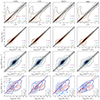 |
Fig. 10. Results for the EDF. Each column represents the results for the methods described in Sect. 3. The first three rows are the labels, with the true value plotted against the predicted one. The fourth column is the MSFS, with true values in red (dashed) and predicted ones in blue (solid). The reported metrics are the NMAD (purple), outlier fraction fout (blue), the bias (green), and for the SFMS the slope (α), the scatter (σ) and fraction of passive galaxies (fp), all defined in Sect. 3.6. |
A significant improvement is observed also for the stellar masses, even without parceling out the fainter galaxies from the Wide-alike, as for the photo-z. This is principally a consequence of the addition of the two IRAC filters and, secondly, of the improved photometry. All the codes show a net improvement for NMADs, outlier fractions, and biases, even for the full set of test galaxies (down to NMADs of ∼0.16 and fout ∼ 13%. If accounting only for the Wide cut, the net improvement gets important, falling to NMAD ∼ 0.12 and fout ∼ 2.5%.
SFRs show a different behavior for the full set of test data. This is due to a particular set of outliers, low star-forming galaxies [log10 (SFR/M⊙ yr−1) < −1] that are mistakenly predicted as higher log10 (SFR/M⊙ yr−1) > 0 due to a wrong photo-z attribution that impacts the SFRs, visible as the strip of ztrue ∼ 1 galaxies in the top panels of Fig. 10. When applying the EWS photometric cuts, the NMADs are lower than those found in the mixed labels Deep – Wide case. The same applies for fout and the bias.
There is a notable exception, as nnpz is able to reduce the impact of these outliers, to the point where even the full set of test data gives back comparable results to the mixed labels Deep – Wide case and better for the EWS-cut ones. This is both a consequence of a better photo-z estimation and an overall better ability of nnpz in recovering the SFRs given the input set of features, as also observed in Sect. 4.4.
Overall, the MS recovery is optimal in the EDF. Of all the considered methods, CCR and nnpz are the ones returning the best overall results, as the former optimally recovers photo-zs and stellar masses, while the latter recovers the SFRs the best. If we perform a binning in redshift, we observe how the best results are obtained when the stellar masses and SFRs are optimally recovered (as the true redshift is) – thus at 0.8 < z < 1.5 – and worse ones at higher-z, where lots of low-z objects are mistakenly placed at high-z with greatly enhanced stellar masses (and to a lesser extent the SFRs), thus bending the whole relation by a significant amount (see rightmost plot in Fig. 11). At lower-z, we notice a symmetric issue, with lots of low-mass and log10 (SFR/M⊙ yr−1) ∼ 0 galaxies removed from the binning as the models place those at z > 2, and thus the predicted relation differs significantly from the true one.
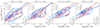 |
Fig. 11. Results for the recovered SFMS in the EDF, in four different redshift bins. Test values are in red (dashed) and predicted ones in blue (solid). The reported metrics are defined in Sect. 3.6. |
There are reasons for optimism. First of all, we stress that these results should be considered lower-limit performance. Forty ROS are the minimum number expected for the EDF, with the highest going up to 53. We expect that increasing the number of ROS will produce better performance, at least slightly (the order of a few percentage points), even though it is not straightforward to assess as mentioned before. In fact, the improvement in metrics seems to saturate after a certain number of ROS. We can roughly quantify, by extrapolating from the different realizations of the metrics for the four different number of ROS used in this work, a reduction of a few percentage points in NMAD and fout with 53 ROS, both with template-fitting and ML methods.
All those results are limited to the UNIONS+Euclid+two IRAC filters, which do not extend over the 4.5 μm observed-frame, with a gap between the HE band and IRAC. The more the galaxies move to higher redshift, the more these particular sets of features will probe the source UV-rest frame, which is less sensible to stellar masses and more to SFRs. However, the EDF, given their extension and importance in galaxy formation and evolution, will benefit from a wealth of ancillary and upcoming multiwavelength data from UV to radio. For example, the EDF-South has been observed with the MeerKAT program MKT-23041 (P.I. Prandoni); the EDF-N is currently proposed to be observed with the LOFAR2.0 Ultra-Deep Observation (LUDO), whose 2 μJy beam−1 at 150 MHz would translate into one of the deepest radio observations ever, and it has already been observed at 144 MHz with a central rms of 32 μJy beam−1 (Bondi et al. 2024); as illustrated, all the EDF has been covered with Spitzer at 3.6 and 4.5 μm (Euclid Collaboration 2022a); deep observations in U band with CFHT (Euclid Collaboration 2024i) are currently ongoing; the same for deep optical observations with Hyper Suprime Cam (Euclid Collaboration 2024e); K band observations with VISTA of the EDF-S have been taken as part of the EDFS-Ks program, down to a limiting magnitude of 23.5 (PI Nonino), covering the gap between the HE band and IRAC. Extending the feature space with mid-IR to submillimeter and radio fluxes will undoubtedly produce better, more reliable physical parameters than those reported in this work.
5. Summary
Euclid and the forthcoming large-scale surveys – Rubin/LSST, Roman) – will benefit from unprecedentedly sampled areas of the sky, with an estimated number of observed sources up to the order of billions. At those scales, automated, accurate, and rapid methods to assess photometric redshifts and physical properties from the observables must be developed and tested.
In this study, we evaluated the performance of Phosphoros, a template-fitting algorithm, with four ML methods for the recovery of photo-zs, stellar masses, star formation rates, and the SFMS: two CatBoost-based methods roote GBDT, a single-pass regressor (CSMR) and a chained regressor ensemble (CCR); a simple and plain DLNN; and nnpz, an enhanced nearest-neighbors algorithm capable of handling the full parameter posteriors. As it is typical in ML applications, the quality of the recovered labels is inevitably limited by the number and quality of input information entering the model. Noisy features hamper a plain association between those and the labels, degrading the final performance.
In order to realistically quantify how reliable Euclid photo-zs and physical parameters will be, we simulated observations of both the EWS and the EDF with ground-based ugriz and Euclid filters (plus two IRAC channels for the latter). The simulations are obtained within the MAMBO workflow, an empirical method to extract galaxies’ physical information from simulated lightcones. We also simulated an intermediate number of ROS mimicking what is expected from the Euclid auxiliary fields, observations of well-known fields in the sky where a wealth of ancillary multiwavelength data is available for optimal photometric and color calibration. Finally, we run all the methods on an unperturbed version of the mocks, that is, without any photometric noise added and trained on the labels true values, serving as an unrealistic best-case scenario for the performance given that particular set of features (magnitudes and pairwise differences, the colors).
We found how, in the unperturbed catalog, that set of 45 features is more than enough for the models to almost perfectly recover photometric redshifts and stellar masses (NMAD < 0.03, fout < 0.3%). Things are more complicated for star formation rates, with NMADs never falling below 0.16. This is expected, as the SFR correlates weakly with the input labels that sample the 0.3–1.8 μm observed-frame wavelength range but correlates strongly with the 8–1000 μm integrated luminosity (and monochromatic flux in the UV at 2800 Å rest-frame).
When feeding the mock photometry to Phosphoros either for the EWS or the EDF, we observe a typical pattern where the vast majority of outliers are generated by low-z galaxies (z < 1) misplaced at 1.5 < z < 5, with predicted higher values of log10(M⋆/M⊙) > 10 instead of ∼8.5, and log10 (SFR/M⊙ yr−1) > 0.5 instead of −2 < log10 (SFR/M⊙ yr−1) < −1. The SFMS is poorly recovered in the EWS, while better though suboptimal results are observed for the EDF, suggesting the need for better-suited, ad hoc priors to adopt for template-fitting.
As we want to evaluate the ML methods with what Euclid will realistically yield, their EWS and EDF performance are measured training on Phosphoros recovered labels and testing on true values. We also checked the metrics improvement when training on true values – inaccessible in a real scenario, as the ground truth is unknown. Moreover, since we simulated four different versions of the mock catalogs (EWS, EDF, and two auxilliary fields named C16 and C25 from the number of expected ROS), for the EWS we test how a model trained on features and labels coming from deeper photometry fare on the test EWS ground truth values.
We found different results by employing two approaches: in the paired labels approach, we are training the models on a rightly coupled set of features and labels coming respectively from the four catalogs and testing on the EWS ground truth. With this approach, we notice a well-known pattern in ML applications: as there is a mismatch between the training and test features (in terms of noise), it is not guaranteed that a deeper set of features (and labels) would lead to better performance. This is particularly true for stellar masses, as the NMADs and fraction of outliers do not improve significantly (or become even worse, see Table C.1) from training and testing on the EWS to training on deeper photometries and testing on the EWS, with the notable exception of EDF training as it benefits from the addition of two IRAC filters.
Better performance is obtained if we employ a mixed labels approach. In this case, the labels are still the Phosphoros results on photometry coming from the four catalogs, but the training features are always the ones from the EWS. Despite the reduction in the training sample size (as only EWS detected sources are employed in training) from a few million to ∼500 k sources, this approach avoids the data mismatch issue, as the features always come from the EWS simulated catalog. More importantly, it acts as a prior on the features-labels association, as the models are able to better distinguish between similar cases near degenerate regions of the feature space, for instance, the ones that generate the outlier cloud of close and less massive galaxies mistaken for far-away and more massive ones.
In fact, those outliers are significantly reduced (or disappear altogether) with this approach. We observed a significant improvement in the performance metrics, matching or even surpassing those obtained with Phosphoros: for nnpz, zphot NMAD decreases from 0.063 to 0.055, and fout is reduced from 22% to 15% passing from Wide training labels to Deep training labels, not so distant from the ideal scenario when the true labels are known (0.047 and 15% respectively). The same goes for stellar masses (for the CCR, NMAD falls from 0.24 to 0.19, outliers from 28% to 11%, while they are 0.14 and 10% in the ideal scenario) and star formation rates (nnpz reaches NMADs of 0.62 starting from 0.71, and outliers of 23% from 30%, lower limits of 0.43 and 11%). The same is true for the MS.
The full EDF would not be finalized until February 2031. In the meantime, the main scientific results will rely on training samples obtained from multiple ROS of the auxiliary fields. We observed how the metrics did not degrade by more than a few percentage points between the C16 and C25 training samples (though here we only use the 9 previously cited bands to infer the results, thus the real ones will benefit from better estimated labels) and the EDF one. Moreover, we also checked how a COSMOS-like reference sample does not significantly impact the model performance, as a reduction to ∼230 k galaxies in the training sample is not enough to degrade those by more than 1–2%. As a final test, we removed the u band filter from the test sample, as we already know that, for DR1, those observations of the southern sky will not yet be available. However, that should not compromise the scientific outcome, as we only notice a small performance degradation, on the order of ∼3%.
As expected, the EDF results are the ones with the best results, where both labels and features come from the deepest available observations (and Phosphoros run on). The parameter recovery is optimal, especially the MS, once considered how the EDF extends the object detection to significantly higher redshifts (one order of magnitude more z > 4 galaxies) and lower stellar masses and SFRs, with one order of magnitude increase for log10(M⋆/M⊙) < 8 and log10 (SFR/M⊙ yr−1) < 0.
There are some caveats to keep in mind to properly gauge all those results in the right framework. In our simulated catalogs, we are only considering galaxies, thus neglecting the potential impact of misclassified stars, AGN and QSOs, local contaminants, and photometric defects. These will undoubtedly cause a degradation in the considered metrics, at least by a few percent, even though a precise quantitative estimation is nontrivial and outside the scope of this work. The simulated EWS and EDF are built assuming BC03 models; thus, whatever discrepancy might come from what an actual galaxy emission is (or the chosen IMF) will impact the overall performance, again, in a nontrivial way. Also, we are evaluating performance on the EWS and EDF simulated catalogs with nine filters, the ground-based ugriz and four Euclid ones. This is the bare minimum that will be released by Euclid, but we know that, especially for the ∼53 deg2 of the EDF given their importance in the galaxy formation and evolution context, multiple ancillary or forthcoming multiwavelength data will be available to complement the Euclid releases.
As such, we can consider our results as a kind of best-case – as we are not accounting for defects in the catalog, the contamination by AGNs, and the fact that galaxy emission could differ from BC03 models – of the worst-case scenario, as adding more filters, especially in the mid-IR to far-IR, will undeniably improve the performance. These results highlight Euclid’s vast potential in assessing galaxy formation and evolution and could serve as a benchmark for all the upcoming large-area surveys in the next decade.
For some ML methods (i.e., the nearest-neighbors algorithms), there is no training phase (or it could be considered instantaneous training); as such, the sample from which the predictions are inferred is not referred to as the training sample but as the reference sample.
Similarly, both terms are applied to data samples that will not be utilized for the model’s training or as a reference sample. The subtle distinction lies in the utilization of a test sample, specifically employed for evaluating the model’s performance.
In typical ML applications, the relation between the size of the training sample and the quality metrics scales in logarithm scale and saturates after a while; as such, adding (or removing) a factor of two from the training sample could not significantly impact the final metrics.
Acknowledgments
The Euclid Consortium acknowledges the European Space Agency and a number of agencies and institutes that have supported the development of Euclid, in particular the Agenzia Spaziale Italiana, the Austrian Forschungsförderungsgesellschaft funded through BMK, the Belgian Science Policy, the Canadian Euclid Consortium, the Deutsches Zentrum für Luft- und Raumfahrt, the DTU Space and the Niels Bohr Institute in Denmark, the French Centre National d’Etudes Spatiales, the Fundação para a Ciência e a Tecnologia, the Hungarian Academy of Sciences, the Ministerio de Ciencia, Innovación y Universidades, the National Aeronautics and Space Administration, the National Astronomical Observatory of Japan, the Netherlandse Onderzoekschool Voor Astronomie, the Norwegian Space Agency, the Research Council of Finland, the Romanian Space Agency, the State Secretariat for Education, Research, and Innovation (SERI) at the Swiss Space Office (SSO), and the United Kingdom Space Agency. A complete and detailed list is available on the Euclid web site (www.euclid-ec.org). AE, MB, LP, SQ, MT, GDL, VA, JB, SF, MS acknowledge support from the ELSA project. “ELSA: Euclid Legacy Science Advanced analysis tools” (Grant Agreement no. 101135203) is funded by the European Union. Views and opinions expressed are however those of the author(s) only and do not necessarily reflect those of the European Union or Innovate UK. Neither the European Union nor the granting authority can be held responsible for them. UK participation is funded through the UK HORIZON guarantee scheme under Innovate UK grant 10093177. We acknowledge the support from grant PRIN MIUR 2017-20173ML3WW_s. We acknowledge the CINECA award under the ISCRA initiative, for the availability of high performance computing resources and support. M.S. acknowledges support by the Polish National Agency for Academic Exchange (Bekker grant BPN/BEK/2021/1/00298/DEC/1), the State Research Agency of the Spanish Ministry of Science and Innovation under the grants ‘Galaxy Evolution with Artificial Intelligence’ (PGC2018-100852-A-I00) and ‘BASALT’ (PID2021-126838NB-I00). This work was partially supported by the European Union’s Horizon 2020 Research and Innovation program under the Maria Sklodowska-Curie grant agreement (No. 754510). Phosphoros filters are taken from the SVO Filter Profile Service (Rodrigo et al. 2012; Rodrigo & Solano 2020). This research has made use of the Spanish Virtual Observatory (https://svo.cab.inta-csic.es) project funded by MCIN/AEI/10.13039/501100011033/ through grant PID2020-112949GB-I00. In preparation for this work, we used the following codes for Python: Numpy (Harris et al. 2020), Scipy (Virtanen et al. 2020), Scikit-Learn (Pedregosa 2011), Pandas (Wes McKinney 2010), CatBoost (Prokhorenkova et al. 2018), Tensorflow (Abadi et al. 2016), nnpz (Tanaka et al. 2018), Phosphoros (Paltani et al., in prep.).
References
- Abadi, M., Agarwal, A., Barham, P., et al. 2016, arXiv e-prints [arXiv:1603.04467] [Google Scholar]
- Akeson, R., Armus, L., Bachelet, E., et al. 2019, arXiv e-prints [arXiv:1902.05569] [Google Scholar]
- Alsing, J., Peiris, H., Mortlock, D., Leja, J., & Leistedt, B. 2023, ApJS, 264, 29 [NASA ADS] [CrossRef] [Google Scholar]
- Alsing, J., Thorp, S., Deger, S., et al. 2024, ApJS, 274, 12 [NASA ADS] [CrossRef] [Google Scholar]
- Angulo, R. E., & White, S. D. M. 2010, MNRAS, 405, 143 [NASA ADS] [Google Scholar]
- Bell, E. F., & Kennicutt, R. C., Jr. 2001, ApJ, 548, 681 [NASA ADS] [CrossRef] [Google Scholar]
- Bell, E. F., Papovich, C., Wolf, C., et al. 2005, ApJ, 625, 23 [Google Scholar]
- Bondi, M., Scaramella, R., Zamorani, G., et al. 2024, A&A, 683, A179 [NASA ADS] [CrossRef] [EDP Sciences] [Google Scholar]
- Bonjean, V., Aghanim, N., Salomé, P., et al. 2019, A&A, 622, A137 [NASA ADS] [CrossRef] [EDP Sciences] [Google Scholar]
- Bowles, M., Scaife, A. M. M., Porter, F., Tang, H., & Bastien, D. J. 2021, MNRAS, 501, 4579 [CrossRef] [Google Scholar]
- Brescia, M., Cavuoti, S., D’Abrusco, R., Longo, G., & Mercurio, A. 2013, ApJ, 772, 140 [NASA ADS] [CrossRef] [Google Scholar]
- Bruzual, G., & Charlot, S. 2003, MNRAS, 344, 1000 [NASA ADS] [CrossRef] [Google Scholar]
- Calzetti, D., Armus, L., Bohlin, R. C., et al. 2000, ApJ, 533, 682 [NASA ADS] [CrossRef] [Google Scholar]
- Carvajal, R., Matute, I., Afonso, J., et al. 2023, A&A, 679, A101 [NASA ADS] [CrossRef] [EDP Sciences] [Google Scholar]
- Cavuoti, S., Tortora, C., Brescia, M., et al. 2017, MNRAS, 466, 2039 [Google Scholar]
- Chabrier, G. 2003, PASP, 115, 763 [Google Scholar]
- Chambers, K. C., Magnier, E. A., Metcalfe, N., et al. 2016, arXiv e-prints [arXiv:1612.05560] [Google Scholar]
- Collister, A. A., & Lahav, O. 2004, PASP, 116, 345 [NASA ADS] [CrossRef] [Google Scholar]
- Cropper, M., Pottinger, S., Niemi, S., et al. 2016, SPIE Conf. Ser., 9904, 99040Q [NASA ADS] [Google Scholar]
- Cunha, P. A. C., & Humphrey, A. 2022, A&A, 666, A87 [NASA ADS] [CrossRef] [EDP Sciences] [Google Scholar]
- Daddi, E., Dickinson, M., Morrison, G., et al. 2007, ApJ, 670, 156 [NASA ADS] [CrossRef] [Google Scholar]
- Dark Energy Survey Collaboration (Abbott, T., et al.) 2016, MNRAS, 460, 1270 [Google Scholar]
- Davidzon, I., Jegatheesan, K., Ilbert, O., et al. 2022, A&A, 665, A34 [NASA ADS] [CrossRef] [EDP Sciences] [Google Scholar]
- Delli Veneri, M., Cavuoti, S., Brescia, M., Longo, G., & Riccio, G. 2019, MNRAS, 486, 1377 [Google Scholar]
- Dieleman, S., Willett, K. W., & Dambre, J. 2015, MNRAS, 450, 1441 [NASA ADS] [CrossRef] [Google Scholar]
- D’Isanto, A., & Polsterer, K. L. 2018, A&A, 609, A111 [Google Scholar]
- Euclid Collaboration (Desprez, G., et al.) 2020, A&A, 644, A31 [EDP Sciences] [Google Scholar]
- Euclid Collaboration (Moneti, A., et al.) 2022a, A&A, 658, A126 [NASA ADS] [CrossRef] [EDP Sciences] [Google Scholar]
- Euclid Collaboration (Schirmer, M., et al.) 2022b, A&A, 662, A92 [NASA ADS] [CrossRef] [EDP Sciences] [Google Scholar]
- Euclid Collaboration (Bisigello, L., et al.) 2023, MNRAS, 520, 3529 [NASA ADS] [CrossRef] [Google Scholar]
- Euclid Collaboration (Aussel, B., et al.) 2024a, A&A, 689, A274 [NASA ADS] [CrossRef] [EDP Sciences] [Google Scholar]
- Euclid Collaboration (Cropper, M., et al.) 2024b, A&A, in press https://doi.org/10.1051/0004-6361/202450996 [Google Scholar]
- Euclid Collaboration (Jahnke, K., et al.) 2024c, A&A, in press https://doi.org/10.1051/0004-6361/202450786 [Google Scholar]
- Euclid Collaboration (Leuzzi, L., et al.) 2024d, A&A, 681, A68 [NASA ADS] [CrossRef] [EDP Sciences] [Google Scholar]
- Euclid Collaboration (McPartland, C. J. R., et al.) 2024e, A&A, submitted [arXiv:2408.05275] [Google Scholar]
- Euclid Collaboration (Mellier, Y., et al.) 2024f, A&A, in press https://doi.org/10.1051/0004-6361/202450810 [Google Scholar]
- Euclid Collaboration (Paltani, S., et al.) 2024g, A&A, 681, A66 [NASA ADS] [CrossRef] [EDP Sciences] [Google Scholar]
- Euclid Collaboration (Scaramella, R., et al.) 2024h, A&A, 662, A112 [NASA ADS] [Google Scholar]
- Euclid Collaboration (Zalesky, L., et al.) 2024i, A&A, submitted [arXiv:2408.05296] [Google Scholar]
- Fazio, G. G., Hora, J. L., Allen, L. E., et al. 2004, ApJS, 154, 10 [Google Scholar]
- Firth, A. E., Lahav, O., & Somerville, R. S. 2003, MNRAS, 339, 1195 [NASA ADS] [CrossRef] [Google Scholar]
- Flaugher, B., Diehl, H. T., Honscheid, K., et al. 2015, AJ, 150, 150 [Google Scholar]
- Galametz, A., Saglia, R., Paltani, S., Apostolakos, N., & Dubath, P. 2017, A&A, 598, A20 [NASA ADS] [CrossRef] [EDP Sciences] [Google Scholar]
- Gentile, F., Tortora, C., Covone, G., et al. 2022, MNRAS, 510, 500 [Google Scholar]
- Gentile, F., Tortora, C., Covone, G., et al. 2023, MNRAS, 522, 5442 [NASA ADS] [CrossRef] [Google Scholar]
- Girelli, G. 2021, Ph.D. Thesis, Alma Mater Studiorum Università, Italy [Google Scholar]
- Girelli, G., Bolzonella, M., & Cimatti, A. 2019, A&A, 632, A80 [NASA ADS] [CrossRef] [EDP Sciences] [Google Scholar]
- Girelli, G., Pozzetti, L., Bolzonella, M., et al. 2020, A&A, 634, A135 [NASA ADS] [CrossRef] [EDP Sciences] [Google Scholar]
- Grazian, A., Fontana, A., Santini, P., et al. 2015, A&A, 575, A96 [NASA ADS] [CrossRef] [EDP Sciences] [Google Scholar]
- Guarneri, F., Calderone, G., Cristiani, S., et al. 2021, MNRAS, 506, 2471 [NASA ADS] [CrossRef] [Google Scholar]
- Harris, C. R., Millman, K. J., van der Walt, S. J., et al. 2020, Nature, 585, 357 [NASA ADS] [CrossRef] [Google Scholar]
- Henriques, B. M. B., White, S. D. M., Thomas, P. A., et al. 2015, MNRAS, 451, 2663 [Google Scholar]
- Hezaveh, Y. D., Perreault Levasseur, L., & Marshall, P. J. 2017, Nature, 548, 555 [Google Scholar]
- Hildebrandt, H., Arnouts, S., Capak, P., et al. 2010, A&A, 523, A31 [NASA ADS] [CrossRef] [EDP Sciences] [Google Scholar]
- Huertas-Company, M., Gravet, R., Cabrera-Vives, G., et al. 2015, ApJS, 221, 8 [NASA ADS] [CrossRef] [Google Scholar]
- Ibata, R. A., McConnachie, A., Cuillandre, J.-C., et al. 2017, ApJ, 848, 128 [Google Scholar]
- Ilbert, O., McCracken, H. J., Le Fèvre, O., et al. 2013, A&A, 556, A55 [NASA ADS] [CrossRef] [EDP Sciences] [Google Scholar]
- Ivezic, Z., Axelrod, T., Brandt, W. N., et al. 2008, Serb. Astron. J., 176, 1 [Google Scholar]
- Kennicutt, R. C., & Evans, N. J. 2012, ARA&A, 50, 531 [NASA ADS] [CrossRef] [Google Scholar]
- Kingma, D. P., & Ba, J. 2014, arXiv e-prints [arXiv:1412.6980] [Google Scholar]
- Laureijs, R., Amiaux, J., Arduini, S., et al. 2011, arXiv e-prints [arXiv:1110.3193] [Google Scholar]
- Leistedt, B., Alsing, J., Peiris, H., Mortlock, D., & Leja, J. 2023, ApJS, 264, 23 [NASA ADS] [CrossRef] [Google Scholar]
- Li, R., Napolitano, N. R., Feng, H., et al. 2022a, A&A, 666, A85 [NASA ADS] [CrossRef] [EDP Sciences] [Google Scholar]
- Li, C., Zhang, Y., Cui, C., et al. 2022b, MNRAS, 509, 2289 [Google Scholar]
- López-López, X., Bolzonella, M., Pozzetti, L., et al. 2024, A&A, 691, A136 [NASA ADS] [CrossRef] [EDP Sciences] [Google Scholar]
- LSST Science Collaboration (Abell, P. A., et al.) 2009, arXiv e-prints [arXiv:0912.0201] [Google Scholar]
- Maciaszek, T., Ealet, A., Jahnke, K., et al. 2016, SPIE Conf. Ser., 9904, 99040T [NASA ADS] [Google Scholar]
- Merlin, E., Fontana, A., Castellano, M., et al. 2018, MNRAS, 473, 2098 [Google Scholar]
- Miyazaki, S., Komiyama, Y., Kawanomoto, S., et al. 2018, PASJ, 70, S1 [NASA ADS] [Google Scholar]
- Mucesh, S., Hartley, W. G., Palmese, A., et al. 2021, MNRAS, 502, 2770 [NASA ADS] [CrossRef] [Google Scholar]
- Nair, V., & Hinton, G. E. 2010, ICML 2010, 807 [Google Scholar]
- Oke, J. B., & Gunn, J. E. 1983, ApJ, 266, 713 [NASA ADS] [CrossRef] [Google Scholar]
- Pasquet, J., Bertin, E., Treyer, M., Arnouts, S., & Fouchez, D. 2019, A&A, 621, A26 [NASA ADS] [CrossRef] [EDP Sciences] [Google Scholar]
- Pedregosa, F., Varoquaux, G., Gramfort, A., et al. 2011, J. Mach. Learn. Res., 12, 2825 [Google Scholar]
- Peng, Y.-J., Lilly, S. J., Kovač, K., et al. 2010, ApJ, 721, 193 [Google Scholar]
- Pozzetti, L., Bolzonella, M., Zucca, E., et al. 2010, A&A, 523, A13 [NASA ADS] [CrossRef] [EDP Sciences] [Google Scholar]
- Prokhorenkova, L., Gusev, G., Vorobev, A., Dorogush, A. V., & Gulin, A. 2018, Adv. Neural Inf. Process. Syst., 31, 6638 [Google Scholar]
- Razim, O., Cavuoti, S., Brescia, M., et al. 2021, MNRAS, 507, 5034 [NASA ADS] [CrossRef] [Google Scholar]
- Rodighiero, G., Renzini, A., Daddi, E., et al. 2014, MNRAS, 443, 19 [Google Scholar]
- Rodrigo, C., & Solano, E. 2020, XIV.0 Scientific Meeting (virtual) of the Spanish Astronomical Society, 182 [Google Scholar]
- Rodrigo, C., Solano, E., & Bayo, A. 2012, SVO Filter Profile Service Version 1.0, IVOA Working Draft [CrossRef] [Google Scholar]
- Salpeter, E. E. 1955, ApJ, 121, 161 [Google Scholar]
- Sawicki, M. 2012, PASP, 124, 1208 [NASA ADS] [CrossRef] [Google Scholar]
- Schreiber, C., Elbaz, D., Pannella, M., et al. 2017, A&A, 602, A96 [NASA ADS] [CrossRef] [EDP Sciences] [Google Scholar]
- Scoville, N., Aussel, H., Brusa, M., et al. 2007, ApJS, 172, 1 [Google Scholar]
- Signor, T., Rodighiero, G., Bisigello, L., et al. 2024, A&A, 685, A127 [NASA ADS] [CrossRef] [EDP Sciences] [Google Scholar]
- Simet, M., Chartab, N., Lu, Y., & Mobasher, B. 2021, ApJ, 908, 47 [NASA ADS] [CrossRef] [Google Scholar]
- Springel, V., White, S. D. M., Jenkins, A., et al. 2005, Nature, 435, 629 [Google Scholar]
- Surana, S., Wadadekar, Y., Bait, O., & Bhosale, H. 2020, MNRAS, 493, 4808 [NASA ADS] [CrossRef] [Google Scholar]
- Tagliaferri, R., Longo, G., Andreon, S., et al. 2003, Lect. Notes Comput. Sci., 2859, 226 [NASA ADS] [CrossRef] [Google Scholar]
- Tanaka, M., Coupon, J., Hsieh, B.-C., et al. 2018, PASJ, 70, S9 [Google Scholar]
- Thorp, S., Alsing, J., Peiris, H. V., et al. 2024, ApJ, accepted [arXiv:2406.19437] [Google Scholar]
- Tuccillo, D., Huertas-Company, M., Decencière, E., et al. 2018, MNRAS, 475, 894 [NASA ADS] [CrossRef] [Google Scholar]
- Ucci, G., Ferrara, A., Pallottini, A., & Gallerani, S. 2018, MNRAS, 477, 1484 [Google Scholar]
- Virtanen, P., Gommers, R., Oliphant, T. E., et al. 2020, Nat. Methods, 17, 261 [Google Scholar]
- Weaver, J. R., Kauffmann, O. B., Ilbert, O., et al. 2022, ApJS, 258, 11 [NASA ADS] [CrossRef] [Google Scholar]
- Werner, M. W., Roellig, T. L., Low, F. J., et al. 2004, ApJS, 154, 1 [NASA ADS] [CrossRef] [Google Scholar]
- Wes McKinney 2010, in Proceedings of the 9th Python in Science Conference, eds. S. van der Walt, & J. Millman, 56 [CrossRef] [Google Scholar]
- Williams, R. J., Quadri, R. F., Franx, M., van Dokkum, P., & Labbé, I. 2009, ApJ, 691, 1879 [NASA ADS] [CrossRef] [Google Scholar]
Appendix A: Feature importances
In this appendix, we present the feature importance for models evaluated with CSMR. In standard ML terminology, feature importance refers to the quantification of the impact each feature has on the model’s predictions. This is measured by considering the number of times a feature is used for splits across all trees in the ensemble and the corresponding improvement in the model’s performance. The higher the number of times a feature is used and the greater the improvement, the more important the feature is considered, giving insights into the relative significance of different features in the data, for example, if and what certain filter or color is more important in correctly assessing a galaxy redshift, stellar mass, or star formation rate.
These findings are reported in Fig. A.1, where we show the feature importance for four different models, each one specifically trained to recover a single label, whether is zphot, log10(M⋆/M⊙), or log10 (SFR/M⊙ yr−1), and a model trained on a set of pooled labels. In each case, to remove altogether every source of noise skewing the results, we are performing the training on the unperturbed catalog (see Sect. 4.3 for further details).
As expected, considering that most of the training galaxies are at 0 < z < 1.5, the HE band is by far the most important one in determining a galaxy’s stellar mass (more than half importance); similarly, for photometric redshifts, the colors hold the most importance, more than single filter observations. Things are more mixed for star formation rates, as with the exception of HE (∼25%), all the other features hold similar importance (between 3% and 6%). When considering all the labels together, we observe a mix between the previous results, with HE being still the most considered feature at ∼25% importance, followed by the colors.
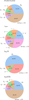 |
Fig. A.1. Pie chart highlighting the most important features in recovering the pooled labels with CSMR. The feature importance weights (in percentage) how much a single feature influences the final prediction. In the Pooled Labels and log10 SFR only cases, 45 features enter the model (magnitudes and all possible color permutations), only five have an importance over 5%. |
Appendix B: Phosphoros results for the calibration fields
In Sect. 4.2, we reported the template-fitting results with Phosphoros to the EWS and EDF. In Fig. B.1, we report the corresponding Phosphoros run to the auxiliary fields at 16 and 25 ROS each. As expected, the performance is intermediate between the EDF and the EWS, though closer to the former. Anyway, it should always be kept in mind that the deeper the observations, the more distant and/or less massive galaxies will enter the catalogs, whose photometric redshifts and physical parameters are harder to properly assess, therefore reducing the expected metrics improvement.
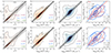 |
Fig. B.1. Phosphoros results on two simulated Euclid auxiliary fields, with 16 (C16, bottom panel) and 25 (C25, bottom panel) ROS each. The ground truth is plotted against the Phosphoros recovered parameters. The black line is the 1:1 relation; the shaded area is the region beyond which a prediction is an outlier. In every plot, the four contours are the area containing 98%, 86%, 39% (corresponding to the 3σ, 2σ and 1σ levels for a 2D histogram) and 20% of the sample. For SFMS the true distribution is reported in red (dashed), the predicted one in blue (solid). The lines are the ODR best-fit to the (passive-removed) distribution. The reported metrics are NMAD (purple), the outlier fraction fout (blue) and the bias (green) for the photometric redshifts and physical parameters, as well as the slope m, scatter σ and fraction of passive galaxies fp for the SFMS, all defined in Sect. 3.6. |
Appendix C: Results with the paired labels approach
In Tabs. C.1–C.2, we report the results for the EWS with the paired labels approach. As described in Sect. 4.4, with this approach, we train each model with a set of features and labels obtained from the Phosphoros run to the corresponding depth (e.g., C16 features, labels from Phosphoros run to the C16 photometry), and test on Wide features and ground truth values obtained from the simulation.
Metrics for the EWS, with the paired labels approach.
Metrics for the recovered SFMS in the EWS, with the paired labels approach.
All Tables
All Figures
|
Fig. 1. Throughput of the filters used through this work. On the top panel we show the four Euclid filters: IE, YE, JE, and HE, along with two IRAC filters at 3.6 μm and 4.5 μm. In the bottom panel, we include the four UNIONS filters that will complement the Euclid data in the northern sky: CFIS u and r, HSC g and z, and PAN-STARRS i. |
| In the text | |
|
Fig. 2. Four simulated Euclid catalogs used in this work (solid purple line, EWS; dashed orange line, C16; solid gray line, C25; dashed-dotted blue line, EDF) shown as the number of sources as a function of the EuclidHE band magnitude (leftmost panel), redshift (center left), stellar mass (center right), and star formation rate (rightmost panel). We notice that the magnitude cut upon which the fields are built is an OR condition on the S/N in HE, IE filters; as such, simulated galaxies are found below the nominal limiting magnitude cut for HE band, as those are detected at S/N > 10 in IE. |
| In the text | |
|
Fig. 3. Phosphoros results on two simulated Euclid catalogs, EWS (top panels) and EDF (bottom panels), with true values plotted against the Phosphoros recovered ones. The black line is the 1:1 relation; the shaded area is the region beyond which a prediction is an outlier. In every plot, the four contours are the area containing 98%, 86%, 39% (corresponding to the 3σ, 2σ and 1σ levels for a 2D histogram) and 20% of the sample. For SFMS the true distribution is reported in red (dashed), the predicted one in blue (solid). The lines are the ODR best-fit to the (passive-removed) distribution. The reported metrics are NMAD (purple), the outlier fraction fout (blue) and the bias (green) for the photometric redshifts and physical parameters, and the slope m, scatter σ and fraction of passive galaxies fp for the SFMS, all defined in Sect. 3.6. |
| In the text | |
|
Fig. 4. Flowchart followed for the reported results on the EWS and EDF. Panel (a) summarizes what has been done for the EWS. In this case, we employed two different approaches: pairing features to labels coming from Phosphoros results at the corresponding depth (paired labels), or with features always from the Wide simulated catalog and labels coming from Phosphoros results at the Calibration and Deep fields depth for the corresponding sources (mixed labels). These pairs of (features, labels) – or (features, posteriors for nnpz (see Sect. 3.4) – are thus given as input for the ML models described in Sect. 3. Panel (b) illustrates the straighter flowchart for the EDF, where the pairs (features, labels) or (features, posteriors) always come from the simulated Deep field. |
| In the text | |
|
Fig. 5. Results for the EWS with the mixed labels approach. The true values on the x-axis are plotted against the predicted values on y. The black line is the 1:1 relation; the shaded area is the region beyond which a prediction is an outlier. Contours are the area containing 98%, 86%, 39% (corresponding to the 3σ, 2σ and 1σ levels for a 2D histogram) and 20% of the sample. Each column represents the results for the methods described in Sect. 3. In the first four rows, the training labels are the recovered ones, coming from Phosphoros results to the mock photometry at the same depth of the field reported in the leftmost plot legend and tested on the EWS (see Sect. 2 for further details). The T.lab Wide-Wide case is exactly the same as the Wide-Wide case in Table C.1. In the fifth row, we show the results of the EWS training the models with their true labels as the best-case scenario for that particular field. The reported metrics are NMAD (purple), the outlier fraction fout (blue) and the bias (green) for the photometric redshifts and physical parameters, as well as the slope m, scatter σ and fraction of passive galaxies fp for the SFMS, all defined in Sect. 3.6). |
| In the text | |
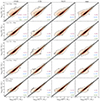 |
Fig. 6. Same as in Fig. 5, but for stellar masses. |
| In the text | |
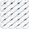 |
Fig. 7. Same as in Fig. 5, but for star formation rates. |
| In the text | |
|
Fig. 8. Same as in Fig. 5, but for the SFMS. Dashed red contours are the test SFMS (i.e., the true values), solid blue is the predicted one. Contour levels are the same as reported in Fig. 5. The lines are the ODR best-fit to the passive-removed distribution (dashed for test SFMS, solid for predicted). The reported metrics are the SFMS slope, scatter, and fraction of passive galaxies, defined in Sect. 3.6. |
| In the text | |
|
Fig. 9. Stellar masses (top panel) and SFRs (bottom panel), color coded with the difference between the true and predicted redshifts, for the nnpz results in the EWS trained with wide features (the upper-right plots in Figs. 6–7). Similar results are obtained for all the other methods considered. The black line is the 1:1 relation. Shaded area is the region beyond which a prediction is an outlier (0.4 dex for stellar masses, 0.8 dex for SFRs, see Sect. 3.6). Contours are the area containing 98%, 86%, 39% (corresponding to the 3σ, 2σ and 1σ levels for a 2D histogram) and 20% of the sample. The zpred − ztrue are measured as the median of the values falling in each true vs predicted bin. It is clearly visible how the wrong photo-z attribution generates the main bulk of catastrophic outliers. However, the distribution scatter along the 1:1 relation – i.e., the NMAD – is mainly due to the inherent difficulties of the methods in assigning the correct PPs given the set of input features independently from the inferred photo-z. This is particularly true for SFRs. This plot also illustrates how penalizing a 0.3 dex definition for catastrophic outliers would be with respect with the ones chosen for this work, which actually follows better the distribution of true and predicted PPs. |
| In the text | |
|
Fig. 10. Results for the EDF. Each column represents the results for the methods described in Sect. 3. The first three rows are the labels, with the true value plotted against the predicted one. The fourth column is the MSFS, with true values in red (dashed) and predicted ones in blue (solid). The reported metrics are the NMAD (purple), outlier fraction fout (blue), the bias (green), and for the SFMS the slope (α), the scatter (σ) and fraction of passive galaxies (fp), all defined in Sect. 3.6. |
| In the text | |
|
Fig. 11. Results for the recovered SFMS in the EDF, in four different redshift bins. Test values are in red (dashed) and predicted ones in blue (solid). The reported metrics are defined in Sect. 3.6. |
| In the text | |
|
Fig. A.1. Pie chart highlighting the most important features in recovering the pooled labels with CSMR. The feature importance weights (in percentage) how much a single feature influences the final prediction. In the Pooled Labels and log10 SFR only cases, 45 features enter the model (magnitudes and all possible color permutations), only five have an importance over 5%. |
| In the text | |
|
Fig. B.1. Phosphoros results on two simulated Euclid auxiliary fields, with 16 (C16, bottom panel) and 25 (C25, bottom panel) ROS each. The ground truth is plotted against the Phosphoros recovered parameters. The black line is the 1:1 relation; the shaded area is the region beyond which a prediction is an outlier. In every plot, the four contours are the area containing 98%, 86%, 39% (corresponding to the 3σ, 2σ and 1σ levels for a 2D histogram) and 20% of the sample. For SFMS the true distribution is reported in red (dashed), the predicted one in blue (solid). The lines are the ODR best-fit to the (passive-removed) distribution. The reported metrics are NMAD (purple), the outlier fraction fout (blue) and the bias (green) for the photometric redshifts and physical parameters, as well as the slope m, scatter σ and fraction of passive galaxies fp for the SFMS, all defined in Sect. 3.6. |
| In the text | |
Current usage metrics show cumulative count of Article Views (full-text article views including HTML views, PDF and ePub downloads, according to the available data) and Abstracts Views on Vision4Press platform.
Data correspond to usage on the plateform after 2015. The current usage metrics is available 48-96 hours after online publication and is updated daily on week days.
Initial download of the metrics may take a while.