| Issue |
A&A
Volume 696, April 2025
|
|
|---|---|---|
| Article Number | A110 | |
| Number of page(s) | 18 | |
| Section | Extragalactic astronomy | |
| DOI | https://doi.org/10.1051/0004-6361/202453068 | |
| Published online | 09 April 2025 | |
Exploring the physical properties of type II quasar candidates at intermediate redshifts with CIGALE
1
Departamento de Física e Astronomia, Faculdade de Ciências, Universidade do Porto, Rua do Campo Alegre 687, PT4169-007 Porto, Portugal
2
Instituto de Astrofísica e Ciências do Espaço, Universidade do Porto, CAUP, Rua das Estrelas, PT4150-762 Porto, Portugal
3
DTx – Digital Transformation CoLab, Building 1, Azurém Campus, University of Minho, PT4800-058 Guimarães, Portugal
4
INAF–Osservatorio Astronomico di Padova, Vicolo dell’Osservatorio 5, I-35122 Padova, Italy
5
Dipartimento di Fisica e Astronomia “G. Galilei”, Università di Padova, Via Marzolo 8, 35131 Padova, Italy
6
INAF-Osservatorio di Astrofisica e Scienza dello Spazio di Bologna, Via Piero Gobetti 93/3, 40129 Bologna, Italy
⋆ Corresponding author; This email address is being protected from spambots. You need JavaScript enabled to view it.
Received:
19
November
2024
Accepted:
26
February
2025
Abstract
Context. Active galactic nuclei (AGNs) play a vital role in the evolution of galaxies over cosmic time, significantly influencing their star formation and growth. As obscured AGNs are difficult to identify due to obscuration by gas and dust, our understanding of their full impact is still under study. It is essential to investigate their properties and distribution, in particular type II quasars (QSO2s), to comprehensively account for AGN populations and understand how their fraction evolves over time. Such studies provide critical insights into the co-evolution of AGNs and their host galaxies.
Aims. Following our previous study, where a machine learning approach was applied to identify 366 QSO2 candidates from SDSS and WISE surveys (median z ∼ 1.1), we now aim to characterise this QSO2 candidate sample by analysing their spectral energy distributions (SEDs) and deriving their physical properties.
Methods. We estimated relevant physical properties of the QSO2 candidates, including the star formation rate (SFR), stellar mass (M*), AGN luminosity, and AGN fraction, using SED fitting with CIGALE. We compared the inferred properties with analogous populations in the semi-empirical simulation SPRITZ, placing these results in the context of galaxy evolution.
Results. The physical properties derived for our QSO2 candidates indicate a diverse population of AGNs at various stages of evolution. QSO2 candidates cover a wide range in the SFR–M* diagram, with numerous high-SFR sources lying above the main sequence at their redshift, suggesting a link between AGN activity and enhanced star formation. Additionally, we identify a population of apparently quenched galaxies, which may be due to obscured star formation or AGN feedback. Furthermore, the physical parameters of our sample align closely with those of composite systems and type 2 AGNs from SPRITZ, supporting the classification of these candidates as obscured AGNs.
Conclusions. This study confirms that our QSO2 candidates, selected via a machine learning approach, exhibit properties consistent with being AGN-host galaxies. This method can identify AGNs within large galaxy samples by considering AGN fractions and their contributions to the infrared luminosity, going beyond the limitations of traditional colour–colour selection techniques. The diverse properties of our candidates demonstrate the capability of this approach to identify complex AGN-host systems that might otherwise be missed. This shows the help that machine learning can provide in refining AGN classifications and advancing our understanding of galaxy evolution driven by AGN activity with new target selection.
Key words: galaxies: active / galaxies: evolution / galaxies: photometry / quasars: general / quasars: supermassive black holes
© The Authors 2025
 Open Access article, published by EDP Sciences, under the terms of the Creative Commons Attribution License (https://creativecommons.org/licenses/by/4.0), which permits unrestricted use, distribution, and reproduction in any medium, provided the original work is properly cited.
This article is published in open access under the Subscribe to Open model. This email address is being protected from spambots. You need JavaScript enabled to view it. to support open access publication.
1. Introduction
Galaxies and active galactic nuclei (AGNs) have an interlinked relationship, each being potentially able to affect the evolution of the other. An AGN consists of a supermassive black hole (SMBH; 106 − 9 M⊙) with an accretion disk made of dust and gas. As interstellar matter falls under the gravitational influence of the SMBH, the accretion process produces a highly energetic signature observable across the entire electromagnetic spectrum (e.g. Seyfert 1943; Lynden-Bell 1969). AGN feedback, positive or negative, can directly influence galaxy evolution by quenching or enhancing star formation (e.g. Fabian 2012; Aversa et al. 2015). Therefore, the evolution of SMBHs and their host galaxies is intrinsically linked, and both are exemplified by AGN feedback, SMBH growth, and the M − σ relation (e.g. Richstone et al. 1998; Magorrian et al. 1998; Gebhardt et al. 2000; Merritt & Ferrarese 2001a,b; Ferrarese & Ford 2005; Decarli et al. 2010; Alexander & Hickox 2012; Kormendy & Ho 2013; Harrison et al. 2018; López et al. 2023).
Active galactic nucleus unification schemes propose a paradigm where inclination (i.e. the line of sight angle) is responsible for some of the differences in the observed properties of AGNs (Antonucci 1993; Urry & Padovani 1995). Among the simplest AGN unification schemes is the separation of sources into two classes based on the orientation of an obscuring dusty torus with respect to our line of sight: type I, called unobscured AGNs, and type II, called obscured AGNs (AGN2s). Type II quasars (QSO2s) are luminous AGN2s with a dusty torus oriented in such a way that the SMBH accretion disk is hidden from our line of sight (e.g. Padovani et al. 2017; Hickox & Alexander 2018, see references therein for a more complete review). Recent infrared (IR) and sub-millimetre observations introduce a new scenario in which a two-component dusty structure with equatorial and polar features is present and radiation pressure plays an important role (Hönig 2019; Stalevski et al. 2023, and references therein).
The obscuration of the accretion disk at ultraviolet and optical wavelengths acts as a ‘natural coronagraph’, enabling the study of galaxy and AGN co-evolution and the physical properties of the host galaxies, which would be challenging with the often overwhelming glare of the optically luminous accretion disk (e.g. Brusa et al. 2009; Lusso et al. 2011; Symeonidis et al. 2013; Lanzuisi et al. 2017). Therefore, AGN2s are useful for understanding the evolution of galaxies across cosmic time (e.g. Magorrian et al. 1998; Di Matteo et al. 2008; Greene et al. 2011; Bessiere et al. 2012, 2014; Humphrey et al. 2015b; Padovani et al. 2017; Villar Martín et al. 2020, 2021).
Multi-wavelength studies, particularly in the X-ray and IR ranges, are crucial for identifying and studying AGN2s and QSO2s (e.g. Sturm et al. 2006; Mainieri & Cosmos Collaboration 2009; Rigopoulou et al. 2009; Rodríguez et al. 2014; Violino et al. 2016; Lambrides et al. 2020; Carroll et al. 2021; Sokol et al. 2023; Yan et al. 2023). While X-ray observations are highly effective for detecting AGNs and estimating their obscuration (e.g. Brandt & Hasinger 2005; Xue et al. 2011; Liu et al. 2017), heavily obscured sources can sometimes be missed (e.g. Comastri et al. 2011; Donley et al. 2012; Hatcher et al. 2021; Carroll et al. 2021, 2023). Despite this, optical to near-IR (NIR) observations remain the primary method for selecting AGN2s due to the abundance of data (e.g. Hickox et al. 2007; LaMassa et al. 2016). These recent studies show the ongoing importance of multi-wavelength observations in the study of the complexity of the obscured AGN population.
Whenever spectroscopic information is missing, photometric information can provide a useful alternative for studying and deriving physical properties. By taking advantage of different types of spectral energy distribution (SED) models (i.e. empirical, semi-empirical, and theoretical), SED fitting tools can reliably be used to estimate photometric redshifts or constrain physical properties (e.g. Bolzonella et al. 2000; Blain et al. 2003; Polletta et al. 2007; Salvato et al. 2009; Conroy 2013; Pacifici et al. 2023). However, powerful tools also have shortcomings or caveats. For example, SED fitting is very dependent on initial assumptions and is sensitive to the quality and diversity of the photometric data. These factors can introduce uncertainties and biases in the computed properties, requiring careful interpretation and, where possible, complementary data to validate results (e.g. Paulino-Afonso et al. 2022).
The selection of QSO2 sources, in the optical, has relied on a combination of a few emission line properties or subjective qualitative criteria (Zakamska et al. 2003, 2004; Alexandroff et al. 2013; Ross et al. 2014). Although this kind of methodology is extremely valuable for the identification and characterisation of QSO2s, it requires optical spectroscopic information and specific emission lines to be detected or present in the spectrum (e.g. CIVλ1549 or [OIII]λλ4959, 5008).
In Cunha et al. (2024), hereafter C2024, we presented AMELIA, a novel machine learning pipeline that incorporates few-shot learning and generalised stacking to identify QSO2 candidates using optical and IR photometry. In C2024, we used the candidates identified by Alexandroff et al. (2013) with a focus on developing a quick and efficient methodology for identifying ‘hidden’ QSO2 sources in large surveys. We used a combination of photometric magnitudes and optical, IR, and optical-IR colours as input into the machine learning pipeline; this allowed it to learn multiple relationships, bypassing the limitations of typically lossy colour–colour selection criteria.
We identified a sample of 366 QSO2 candidates within the redshift desert (1 ≤ z ≤ 2). The SED fitting Code Investigating GALaxy Emission (CIGALE) was used to estimate the contribution of AGNs to the total IR dust luminosity for the QSO2 candidate sample. In the current study we performed a more comprehensive SED fitting to estimate the host galaxies’ physical properties and contextualise the sources in the overall process of galaxy evolution.
This paper is organised as follows. Section 2 details our photometric data selection and QSO2 candidate selection methodology. In Sect. 3 we describe the SED fitting tools used in this work, along with their setup. Section 4 tests the reliability of photometric redshift estimation using the SED fitting tool LePhare++ with spectroscopic redshifts from the Sloan Digital Sky Survey (SDSS). Section 5 provides the analysis and estimations of the physical properties of the QSO2 candidates using CIGALE. In Sect. 6 we explore the addition of radio and X-ray photometry to the SED fitting and how they influence the derived physical properties. Section 7 investigates the use of the derived star formation rate (SFR) to gain insights into their physical nature. Section 8 compares our results with the current literature. In Sect. 9 we present a comparison with the simulated semi-empirical catalogue Spectro-Photometric Realisations of Infrared-selected Targets (SPRITZ). Finally, Sect. 10 summarises our conclusions. Throughout this paper, we adopt a flat-universe cosmology with H0 = 69.3 km s−1 Mpc−1 and ΩM = 0.286 (WMAP 9-year results, Hinshaw et al. 2013), similar to Yang et al. (2022).
2. Photometric data
We used data from SDSS (Ahumada et al. 2020; Abdurro’uf et al. 2022), Wide-field Infrared Survey Explorer (WISE; Wright et al. 2010), X-ray Multi-Mirror Mission (XMM-Newton; Lin et al. 2012), and the LOw-Frequency ARray (LOFAR) Two-metre Sky Survey (LoTSS; Shimwell et al. 2022). In the following subsections, we describe the different samples used in this study and their motivation.
2.1. Control sample and QSO2 candidates
From the SDSS DR16 spectroscopic galaxy sample, we selected sources based on photometric constraints that meet the following criteria (AB magnitudes): (i) 19 ≤ u ≤ 26; (ii) 19 ≤ g ≤ 24; (iii) 19 ≤ r ≤ 24; (iv) 19 ≤ i ≤ 24; (v) 19 ≤ z ≤ 25. This selection resulted in approximately 22 000 galaxies for identifying QSO2 candidates (see the methodology in Sect. 3 of C2024). These criteria were chosen to emulate the optical observational constraints applied to the class A sample described in Alexandroff et al. (2013), where QSO2 objects are identified by narrow emission lines (e.g. Lyαλ1216 and CIVλ1549), weak continuum, absence of associated absorption features, and high equivalent width (EW), within a redshift range of 2 ≤ z ≤ 4. (For further details on how this sample was used to derive QSO2 candidates, see C2024).
The selected galaxies were then used to identify QSO2 candidates using AMELIA. From this sample, we selected the candidates assuming a QSO2 classification probability ≥0.8. As a final product of our pipeline, we obtained 366 QSO2 candidates, with redshift between 1 and 2, the so-called redshift desert. In C2024, we added further observational evidence for the AGN nature of the QSO2 candidates by comparing photometric colour–colour criteria, performing spectroscopic analysis whenever possible, and estimating the fraction of AGNs using CIGALE.
From the sample of non-QSO2 candidates (i.e. those with a QSO2 classification probability ≤0.5), we randomly extracted 366 galaxies to serve as a control sample. This control sample is expected to reveal distinct properties in the colour–colour photometric space across both optical and IR wavelengths. By comparing their estimated physical properties with those of QSO2 candidates, we can validate the refined selection criteria provided by AMELIA.
2.2. Bongiorno sample
In Bongiorno et al. (2012), obscured AGNs were selected using a [NeV]λ3426-based optical selection, within the zCOSMOS bright survey1 (Lilly et al. 2007). The catalogue presents four classifications derived using spectra – Classsp (class 1), unobscured AGNs (class 2), obscured AGNs classified from the X-ray (class 22.2), and obscured AGNs selected using the Baldwin-Phillips-Terlevich diagram (class 22.4) – as well as obscured AGNs selected through the [NeV] emission line.
Two selection constraints were applied to the Bongiorno sample: 1 ≤ z ≤ 2; and Classsp ≠ 1. The first constraint ensures that the sample is within the redshift range of our candidate sample. The second removes the unobscured AGNs from the sample. The final sample has 87 sources, with 78 sources with class 2 and 9 sources with class 22.4. In the catalogue, the authors also provide stellar mass and SFR estimates derived from photometric SED fitting. This sample will serve as an AGN control group, allowing us to compare the physical properties of our QSO2 candidates.
3. SED fitting
While the use of semi-supervised machine learning-based methodologies can help accelerate astronomical analysis, it is crucial to validate and analyse the output of such methods. Since our QSO2 candidates do not have high S/N spectra available, we based our inference of the physical parameters on the photometric data available. When SED fitting techniques are explored, it can easily transform into a very complex and fascinating problem. In this work, we used the state of the art SED implementations to characterise our candidate sample, while taking into consideration the caveats of only using optical and IR data from SDSS and WISE.
3.1. LePhare++
LePhare++ (Arnouts et al. 1999; Ilbert et al. 2006; Arnouts & Ilbert 2011)2 is an SED fitting code optimised to compute photometric redshifts. It uses a chi-square minimisation approach to compare observed photometric data with theoretical models or SED templates. For each redshift, the code generates model photometry by redshifting the SED templates and integrating them over the filter transmission curves. Through a chi-square minimisation, LePhare++ identifies the best-fit class and redshift, for the observed photometry, and takes into account photometric errors in its calculations (e.g. Hatfield et al. 2022). In this work, LePhare++ will be used to compare photometric redshifts with SDSS spectroscopic redshifts.
In our usage of LePhare++, we took into consideration two outputs based on the chi-square minimisation: best-fit class and redshift. We considered libraries for stars, galaxies and quasi-stellar objects (QSOs). In particular, we are interested in the templates for composite systems, as we expect them to be the more suitable solution for our sample. For this study, we considered a comprehensive set of spectral templates tailored to capture the diversity in galaxy morphologies, AGN contributions, and stellar populations. The templates included a range of hybrid galaxy-AGN models from Salvato et al. (2009), with various percentages of AGN contribution, enabling the modelling of composite galaxies. Additionally, we included templates from Ilbert et al. (2009). Furthermore, a range of stellar templates from Pickles (1998) were used to ensure accurate fitting across spectral types. This diverse template set allows the SED fitting to account for both galaxy and AGN contributions across a wide range of redshifts and physical conditions. We allowed the redshift to vary between 0 and 6, with constants steps δ = 0.1.
3.2. CIGALE
To better characterise our sample, we required a more sophisticated SED fitting code capable of inferring both the physical properties of the host galaxy and the AGN within it. We used CIGALE (version 2022.1; Burgarella et al. 2005; Noll et al. 2009; Boquien et al. 2019; Yang et al. 2022, CIGALE). CIGALE performs the SED fitting within a self-consistent framework that balances UV/optical absorption with IR emission. By analysing the best-fit model, it can estimate various parameters, including the contributions from stellar, AGN, and star formation components, to match the photometric data from the rest-frame UV to the far-IR (FIR) bands.
To model the star formation histories (SFHs) of our target galaxies, we adopted a delayed SFH with an optional exponential burst (sfhdelayed) within CIGALE. This model provides a good balance between simplicity and the ability to capture the key features expected in the SFHs of our sample, which includes both early-type and late-type galaxies. Mathematically, this SFH is represented as
![Mathematical equation: $$ \begin{aligned} \mathrm{SFR}(t) \propto \frac{t}{\tau ^2} \times exp(-t/\tau ), t \in [0,t_0], \end{aligned} $$](/articles/aa/full_html/2025/04/aa53068-24/aa53068-24-eq1.gif) (1)
(1)
where t0 represents the age of the galaxy (i.e. the time since the onset of star formation), and τ corresponds to the time at which the SFR reaches its peak. By adjusting the parameter τ, we can effectively model a range of SFHs, from those with a rapid rise and fall in star formation, small τ, to those with a more gradual evolution, large τ.
This SFH model assumes that star formation begins after a delay, allowing for a period of quiescence before the onset of significant star formation activity (Małek et al. 2018). The optional exponential burst component enables us to account for potential short-lived increases in star formation that may occur.
For the stellar populations, we used the Bruzual & Charlot (2003) single stellar population models with the Chabrier (2003) initial mass function. We assumed solar metallicity (Z = 0.02) for all single stellar population models. To account for the effects of dust on the observed light, we adopted the models from Calzetti et al. (2000) and Leitherer et al. (2002). This approach enables differential reddening between young and old stellar populations, which we separated by an age of 10 Myr. This separation is motivated by the assumption that very young stars are still embedded in their dust-producing birth clouds, whereas older stars have migrated away from these regions. The colour excess of the nebular emission lines, E(B − V), was allowed to vary between 0.1 and 0.9, with a step of 0.1, to explore a range of dust attenuation levels.
Finally, to model the IR emission from dust, we used the model from Dale et al. (2014). This model considers the dust emission as a function of the radiation field intensity (U), with a single parameter, α, controlling the distribution of the dust mass with respect to U.
To account for the potential contribution of an AGN to the overall SED, we included the SKIRTOR model (Stalevski et al. 2012, 2016). This model provides a sophisticated representation of the AGN torus by considering it to be composed of dusty clumps. Specifically, the SKIRTOR model assumes that 97% of the torus mass is distributed in high-density clumps, while the remaining 3% is smoothly distributed. This two-phase distribution enables a more realistic representation of the torus density structure. Additionally, the model accounts for the anisotropic emission from the accretion disk, which is the flattened disk of material spiralling onto the black hole.
To explore a range of possible AGN geometries, we considered four different values for the opening angle (oa) of the torus: 20, 40, 60, and 80 degrees. The opening angle is measured between the equatorial plane of the torus and its outer edge. The half-opening angle of the dust-free region, which represents a clear line of sight towards the central engine, is then defined as 90° − oa. We also varied the inclination parameter, which is the angle between our line of sight and the AGN axis, from 30° to 90°, in steps of 10°. This allows us to account for different viewing angles of the AGN.
For the extinction of light passing through the polar regions of the torus, we adopted the extinction law of polar dust from Gaskell et al. (2004). The amount of extinction in the polar direction, quantified by the colour excess E(B − V), was allowed to vary between 0 and 1 magnitude (see Table A.2).
To quantify the relative contribution of the AGN to the total IR dust luminosity, we used the AGN fraction, fracAGN, defined as
 (2)
(2)
where Ldust, AGN is the luminosity of the dust heated by the AGN, and Ldust, galaxy is the luminosity of the dust heated by stars within the galaxy. Both luminosities are integrated over all wavelengths. We allowed fracAGN to vary from 0 to 0.99, covering a wide range of AGN contributions, from negligible (∼0) to dominant (∼1).
4. Testing the SDSS spectroscopic redshifts
CIGALE requires the redshift to be fixed during the fitting process. It is thus important to validate the spectroscopic redshifts from SDSS, since they are in the redshift desert. While SDSS redshifts in general are reliable, our sample is extreme and shows very noisy spectra, sometimes with clearly wrong redshifts (e.g. Yuan et al. 2016), and in some cases we are unable to see any emission lines, in sources analogous to the ‘line-dark’ radio galaxies (Humphrey et al. 2015a, 2016, see also Sect. 8 of C2024). To assess this reliability, we took two different approaches: spectroscopic validation via spectral stacking; and photometric redshift estimation using LePhare++ SED fitting code.
4.1. Spectral stacking
To apply the spectral stacking technique, we collected the available spectra for the QSO2 sample from SDSS DR17. In total, we obtained 310 spectra, no flags or warnings were considered here, with spectroscopic redshifts derived using idlspec2d. Given the lack of high signal-to-noise ratio spectroscopic data, we did not correct for possible contaminants in the sample when producing the final stacked spectrum. Although some contamination is anticipated due to the sample’s non-pure composition, this does not interfere with one of our main objectives, validating the AGN nature of the sources. Each spectrum was then moved to the rest frame wavelength, normalised by the mean flux, and then summed into a single spectrum after spline-interpolation.
For sources with an identifiable emission line, for example [OII]λλ3727, 3730, if the derived spectroscopic redshift is incorrect, or with a high deviation from the true redshift, we expect the stacked spectrum to have multiple features to appear at unexpected wavelengths. Moreover, small redshift deviations will only produce an artificial broadening effect in the detected emission lines. In contrast, noisy or featureless spectra will be cancelled out during the stacking procedure.
The final stacked spectrum, shown in Fig. 1, reveals a mixture of emission lines, primarily originating from the host galaxies, with a clear detection of the [NeV]λλ3346, 3426 line with S/N ∼ 6.7. The extremities of the spectrum are under-represented due to the redshift distribution, meaning certain features, such as CIII]λ1909 and [OIII]λλ4959, 5007, are only visible in a subset of sources. In the 3900–4300 Å range, the continuum is dominated by noise, probably due to imperfect sky subtraction.
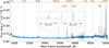 |
Fig. 1. Stacked spectrum of QSO2 candidates with normalised median flux in the rest-frame wavelength, obtained through spline interpolation using available SDSS spectra. The spectrum is additionally normalised based on the number of contributing spectra for each rest-frame wavelength. Grey vertical lines mark the positions of emission lines in the rest frame. The plot includes two zoomed-in regions: (1) 3326–3526 Å, highlighting the [NeV]λ3426 emission line, and (2) 3630–3830 Å, highlighting the [OII]λλ3727, 3730 emission lines. The red line represents the Gaussian fit applied to the spectrum. |
To explore how the redshift might influence emission properties, we measured the EW of the stacked [OII]λλ3727, 3730 line, finding a value of 21.1 ± 2.1 Å. This is in line with the [OII] EW of 18.0 ± 1.8 Å reported by Greene & Ho (2005) for a sample of type 2 Seyfert galaxies, which are associated with lower ionising luminosities. Furthermore, our result is also consistent with the median [OII] EW of 18.8 ± 1.9 Å found in the SDSS QSO2 sample studied by Zakamska et al. (2003) at 0.3 < z < 0.83. Thus, the measured [OII] EW in our stacked spectrum aligns well with previous studies.
4.2. LePhare++: Photometric versus spectroscopic redshift
We estimated the photometric redshifts using the SED fitting code LePhare++ to compared them with the ones derived from SDSS spectra. We divide this study into two parts. First, we compared the LePhare++ photometric redshifts with the spectroscopic redshift derived from the [OII]λλ3727, 3730 emitters. Then we performed the same analysis with the complete QSO2 candidate sample.
To perform this analysis, we considered the following metrics: the normalised median absolute deviation (NMAD),
 (3)
(3)
to compute the variability between measurements, were zspec is the spectroscopic redshift from SDSS and zphot is the photometric redshift derived using LePhare++; the fraction of catastrophic outliers (fout), as defined in Hildebrandt et al. (2010), where a value is considered to be a catastrophic outlier when
 (4)
(4)
and the bias, where the systematic deviations error are calculated as
 (5)
(5)
In Table 1, we present the statistical metrics that compare the zphot derived with LePhare++ to the zspec from SDSS. We performed two analyses that differ in the selection method for zphot: one based on the best χ2 value, choosing between zQSO (if the QSO template is the best fit) or zGAL (if the galaxy template is the best fit), and the other considering only zGAL. The results show that the estimates of zphot tend to be systematically lower than the SDSS zspec, with only a few cases where zphot exceeds the spectroscopic values. This pattern suggests that the combination of optically faint and mid-IR (MIR) enhanced components introduces degeneracies, denigrating the redshift estimation using SED fitting. In Fig. B.1 we show four fitting examples along with their distribution of the probability density function.
Statistical metrics for the photo-z derived using LePhare++, compared with SDSS spectroscopic redshifts, when considering QSO and galaxies templates.
We should point out that for the best-fit template class, we found that 78% of sources are best fitted with an AGN template (including composite systems with an AGN component and QSO templates), 28% of sources are best fitted by a composite template with an AGN component higher than 50%, and 50% are best fitted by a QSO template. This result is consistent with the AGN classification presented in C2024, using CIGALE. Due to the degeneracies observed with the LePhare++zphot, we adopt the spectroscopic redshifts derived by the SDSS pipeline in Sect. 5.
5. CIGALE: Physical property estimations
Here, we present the results of physical property estimation for our QSO2 candidates using CIGALE. The parameter grids for the control sample and the QSO2 candidates are shown in Tables A.1 and A.2, respectively. We took into account the parameters provided in Yang et al. (2020) and modified them according to our needs. The main reason for using two different grids for the control sample and the QSO2 candidates is that, when the same grid was applied to both, we observed that the derived SFRs were hitting a plateau at the upper limit. We found that for our control sample, a more recent starburst (SB) event was required to explain the bright UV emission. Therefore, a more recent SFH was required to successfully fit the control sample and derive its physical properties, compared to the QSO2 candidates. We adjusted the stellar age components for SFH, allowing the inference to converge and provide a more reliable estimation.
5.1. AGN classification with fracAGN
Since CIGALE uses multi-component models to fit the SEDs of galaxies and a Bayesian approach to refine the output properties, it allows well-constrained physical properties and uncertainties to be derived, under the assumption that the models we fit are representative of the sample under consideration. We took advantage of the implementation of the SKIRTOR model to infer the best-fitting parameters related to the AGN component. The AGN model will be of high importance for fitting the enhanced IR emission observed in our candidate sample. In Fig. C.1, we show four examples of the best-fit model using CIGALE.
As previously observed in C2024, the SKIRTOR model consistently estimates a high fracAGN. In this study, we also considered a source to have a substantial AGN contribution when fracAGN > 0.1, following the criteria established by Leja et al. (2018) and Thorne et al. (2022). This criterion is satisfied by all members of our candidate sample, aligning with their AGN classification. Furthermore, we applied the SKIRTOR model to the control sample to study its ability to recover the fracAGN in sources without a considerable AGN contribution. We found that all galaxies within the control sample exhibited a fracAGN ≤ 0.1, consistent with our expectation that these are primarily star-forming (SF) galaxies without a significant AGN contribution.
The specific AGN luminosity is defined as the ratio between the AGN luminosity (LAGN) and the stellar mass (M*): LAGN/M* (Bernhard et al. 2016; Thorne et al. 2022). In Fig. 2, we show a 2D histogram of M* and LAGN/M*, as a function of fracAGN of our sample. While studies focusing on the stellar mass (M*) distribution of QSO2s are limited, Bessiere et al. (2014) estimated the M* of the QSO2 SDSS J002531−104022 to be 4–17 × 1010 M⊙, which is within our derived M* distribution interval.
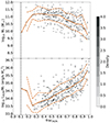 |
Fig. 2. 2D histogram of the stellar mass, M* (top) and specific AGN luminosity, LAGN/M*, defined in Thorne et al. (2022, bottom), as a function of fracAGN for the QSO2 sample. The colour gradient indicates the density of sources for each bin. The median and standard deviation are represented by the solid and dashed orange lines, respectively. The vertical black line indicates the fracAGN > 0.1 threshold used in Leja et al. (2018) to characterise sources with significant AGN contribution. |
When looking at how fracAGN varies with M*, we see that M* decreases as fracAGN increases. This indicates a significant anti-correlation: less massive galaxies tend to have a higher fractional AGN contribution. This trend is supported by a Spearman’s rank correlation coefficient of −0.488 (p < 0.001), showing a moderate negative relationship between the two variables.
Considering that only nine photometric points were used in this study, due to the lack of observations in other wavelength regimes (including FIR), one can argue that CIGALE might be assigning most of the total luminosity to the AGN component, resulting in an underestimation of the stellar mass. We investigated the relationship between AGN activity and stellar mass through two approaches. First, for sources with high AGN contribution (fracAGN > 0.5), the Pearson correlation coefficient between AGN luminosity and stellar mass was −0.02, indicating no significant linear relationship. Second, expanding to the full sample (all fracAGN values), the coefficient was −0.17, showing a very weak negative correlation. A visual inspection of the fracAGN versus AGN luminosity plot, colour-coded by stellar mass, focused on AGN-dominated sources (fracAGN > 0.5), revealed no clear trends or evidence that AGN luminosity affects the estimation of stellar mass.
A possible justification is the role of AGN feedback, through outflows or radiation pressure that can heat and expel gas from the galaxy, effectively suppressing star formation (Harrison & Ramos Almeida 2024). This effect is more significant in galaxies with a higher fracAGN, where the AGN energy output plays a dominant role (e.g. Cresci et al. 2015). The observed anti-correlation remains consistent even when focusing on a subsample of galaxies within a narrow range of M*.
On the other hand, we identify a positive correlation in LAGN/M* with fracAGN. Thorne et al. (2022) also identifies such a trend for sources with fracAGN > 0.8. Since our sample is much smaller and represents a specific subtype of AGNs, we do not expect the same trend in Thorne et al. (2022) to be present. An important caveat to remember is that in this study we only used optical and IR data, from 0.3 to 22 μm. Therefore, because of optical obscuration observed in our sample, we expect the IR part of the SED to dominate, which increases LAGN with fracAGN.
A significant caveat of our study is the absence of FIR data, which would support the derivation of accurate SFRs, as noted by Ciesla et al. (2015). Consequently, the estimation of AGN luminosity would also be improved by incorporating FIR and sub-millimetre data. We conducted a 4″ radius search of the updated Herschel/PACS Point Source Catalogue (Marton et al. 2024) but did not find any counterparts. Since both C2024 and this current work focus on the analysis of QSO2 candidates selected from a large survey focused on the Northern Hemisphere, and therefore covering a significant area of the sky, we are directly impacted by the limited availability of all-sky multi-wavelength data. Thus, our analysis provides a preliminary exploration of the physical properties of our candidate sample, forming the basis for future observational time proposals to further characterise our QSO2 candidates, in the redshift desert.
5.2. SFR–M* diagram
The intrinsic connection between SFR and M* has been extensively discussed in the literature as a key relationship to study and understand galaxy evolution (e.g. Brinchmann & Ellis 2000; Brinchmann et al. 2004; Noeske et al. 2007; Bisigello et al. 2018, and references therein). Schreiber et al. (2015) parameterise the SFR of main sequence (MS) galaxies as a function of redshift and stellar mass:
![Mathematical equation: $$ \begin{aligned} \log _{10}(\mathrm{SFR}_{\mathrm{MS}}[\mathrm{M}_{\odot }/\mathrm{yr}]) = m - m_0 + a_0 r - a_1 \left[\max (0, m - m_1 - a_2 r)\right]^2 ,\end{aligned} $$](/articles/aa/full_html/2025/04/aa53068-24/aa53068-24-eq6.gif) (6)
(6)
with m0 = 0.5 ± 0.07, a0 = 1.5 ± 0.15, a1 = 0.3 ± 0.08, m1 = 0.36 ± 0.3, a2 = 2.5 ± 0.6, r = log10(1 + z) where z is the redshift, and m = log10(M*/109 M⊙). The parameters are physically motivated to preserve the slope increase with redshift and the ‘bending’ effect, verified at low stellar mass and high redshift (see Schreiber et al. 2015, for more details).
In Fig. 3 we plot the SFR–M* diagram for the QSO2 candidates and SDSS galaxies. The star formation MS described by Schreiber et al. (2015), at the mean SDSS spectroscopic redshift of our candidates (z = 1.1), is plotted as a solid line. In the contours, we show the SFR–M* distribution for a sample of 87 X-ray and optically selected AGN2s from the zCOSMOS survey by Bongiorno et al. (2012) with redshift 1 ≤ z ≤ 2. This analysis allows us to understand and compare the distribution of our candidates with confirmed AGN2s. We observe a similar distribution in the SFR–M* diagram, with some candidates having higher M* and SFR. For the SDSS control sample, we observe, on average, a higher SFR estimation within similar M*.
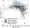 |
Fig. 3. SFR as a function of stellar mass (M*) for the QSO2 candidates (black dots) on a logarithmic scale. The star formation MS described by Schreiber et al. (2015) at the mean SDSS spectroscopic redshift of our candidates (z = 1.1) is shown as a solid line, with dashed lines indicating a 0.4 dex deviation. The contours display the M*–SFR distribution for X-ray and optically selected AGN2s from the zCOSMOS survey by Bongiorno et al. (2012) with redshifts 1 ≤ z ≤ 2 (orange) and for the control sample of SDSS galaxies (blue). |
Zakamska et al. (2003) constructed a sample of 291 QSO2s at redshifts between 0.3 and 0.83 using SDSS spectroscopic data. These sources were identified by their narrow emission lines (FWHM < 2000 km/s), and their high EWs and high-ionisation lines ratios (e.g. [OIII]λ5008/Hβλ4861). We used the available [OII] luminosities3 to compute their SFR using the Kewley et al. (2004) relation:
![Mathematical equation: $$ \begin{aligned} \mathrm{SFR}([\mathrm{OII}])(\mathrm{M_{\odot }\,yr}^{-1}) = (6.58 \pm 1.65) \times 10^{-42} L(\mathrm{[OII]})\,\mathrm{ergs\,s}^{-1} .\end{aligned} $$](/articles/aa/full_html/2025/04/aa53068-24/aa53068-24-eq7.gif) (7)
(7)
In Fig. 4 we plot the difference between the CIGALE estimated SFR and the MS SFR for the QSO2 candidates, the control sample, the Bongiorno sample (Bongiorno et al. 2012), and the Zakamska sample (Zakamska et al. 2003). It is clear that our candidate sample has a broader distribution of SFR, encompassing a mixture of SB to quiescent galaxies. Regarding the higher SFR seen for the control sample, selection bias can play a role here, as for SF galaxies to be detected at these redshifts, the [OII] λλ3727, 3730 lines must be bright, which in itself requires a higher SFR. Finally, we observe that our sample of QSO2 candidates is spread across the SFR–M* diagram, from the SB to the quiescent regime.
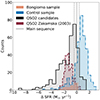 |
Fig. 4. Difference between the estimated SFR and the MS SFR for the QSO2 candidates, the control sample, the Bongiorno sample (Bongiorno et al. 2012), and the Zakamska sample (Zakamska et al. 2003). The solid grey line represents the MS of star formation found by Schreiber et al. (2015) at z = 1.1, and the dashed lines give a scatter of ±0.4 dex. |
6. CIGALE: Multi-wavelength analysis
The SED fitting results presented above are based on optical to MIR photometry, but it is well-known that AGNs have clear signatures outside these wavelength ranges. For a subset of our candidates we can check our SED fitting results by incorporating radio and/or X-ray data, and in the following we discuss the resulting impact on the inferred physical parameters.
6.1. Including LoTSS radio photometry
We tested the inclusion of LoTSS radio photometry (Shimwell et al. 2022) alongside SDSS and WISE data to assess its impact on the fit in CIGALE. A 5″ radius search of our coordinates against the LoTSS Data Release 24 identified matches with 16 sources. Our primary objective was to evaluate how the inclusion of radio data influences the estimation of AGN physical properties, particularly by altering the IR fit and its effect on the inferred galaxy properties.
In Fig. 5, we show the scatter plot with the physical properties with and without radio photometry. Additionally, we show the difference between the physical properties estimated with radio photometry subtracted by those estimated without. We observed that the properties of the host galaxies, M* and SFR, show only slight variations, which do not have a profound impact on the overall study. When including the radio data, the fracAGN and LAGN inferred are somewhat higher than if radio data are excluded. In particular, we see a tendency to estimate a smaller fracAGN. The root cause of this difference is that when including radio data, there is tension between the non-thermal radio model fit and the MIR part of the SED fit, leading to the latter being less well constrained. This signals a potential inconsistency in the MIR to radio modelling and to make progress a more in-depth study of this is needed with potentially updates to the model, this is however outside the bounds of this work.
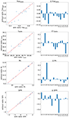 |
Fig. 5. Comparison between physical properties estimated with and without radio LoTSS photometry, using CIGALE. Left: scatter plots comparing the properties of galaxies with and without radio LoTSS photometry, such as the AGN fraction, AGN luminosity, stellar mass, and SFR. All values are provided in logarithmic scale, with the exception of the fracAGN. Each scatter plot includes a 1:1 reference line, as a dashed red line. Right: bar plots of the differences in the same properties, for each source (numbered in the x axis): SDSS+WISE – SDSS+WISE+LoTSS. |
6.2. Including XMM-Newton X-ray photometry
Taking advantage of the flexibility provided by CIGALE, we conducted a similar comparison to evaluate the impact of incorporating X-ray photometry into the SED fitting process. A 2″ radius search for our QSO2 candidates identified matches with five sources. We then integrated the 2–12 keV XMM-Newton photometry (Lin et al. 2012) into CIGALE for analysis.
The comparison study is presented in Fig. 6 (which is similar to Fig. 5), where the physical properties of five X-ray emitters are presented. In this case, we see that the introduction of X-ray data changes the estimated properties for both the AGN and the host galaxy. The least affected parameter is the SFR, which increases for sources with a lower estimated SFR according to SDSS+WISE data. For two of the five sources, the stellar mass estimates when including X-ray data increase by nearly 1 dex, indicating a significant underestimate of the stellar mass when X-rays are included.
The physical properties of AGNs have the highest variance in this study. For two sources, the LAGN is overestimated, according to the one estimated with the addition of X-ray photometry. The most affected property is fracAGN, with two sources having a difference of ∼0.6, resulting in fracAGN ∼ 0.4. Although the AGN contribution remains significant, the observed difference in AGN physical properties arises from the reduced fit to the IR part of the SED when the X-ray model is included. When X-ray photometry is included, the fit places less weight on the MIR, resulting in an underestimate of the MIR emission. This leads to a decrease in fracAGN while compensating for the increase in stellar mass.
7. Separating QSO2 candidates using the SFR
The ratio between SFR and SFRMS allows us to create different regions that separate galaxies into SBs, SF, and quiescent (e.g. Azadi et al. 2015; Aird et al. 2019; Vietri et al. 2022). In our sample, the galaxies are divided into four regimes: SB with log(SFR/SFRMS) > 0.4 dex; SF with log(SFR/SFRMS) ± 0.4 dex; sub-MS with log(SFR/SFRMS) between −0.4 and −1.3; and quiescent with log(SFR/SFRMS) < −1.3 (e.g. Aird et al. 2019; Vietri et al. 2022).
To understand how the quantity SFR/SFRMS relates to the M*, we show the results for our QSO2 candidates in Fig. 7. The sources are colour-coded according to the estimated fracAGN. In summary, we obtain 31 sources in the SB region (∼8.49%); 88 sources in the SF region (∼24.11%); 98 sources in the sub-MS region (∼26.85%); and 148 sources in the quiescent region (∼40.55%). The candidates in the quiescent region are among the most massive candidates with M* within the range 1010.5 − 12 M⊙, while the SB and MS regions show a wider M* range. Similarly to the results of Vietri et al. (2022), we do verify a preference for massive host galaxies (M* ≥ 1010 M⊙) to have a lower SFR.
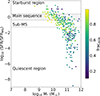 |
Fig. 7. Measurements of the logarithm of the ratio SFR/SFRMS as a function of the logarithm of stellar mass, M*. The SFRs relative to the MS of star formation for galaxies were computed assuming the average redshift from our QSO2 candidate sample, z = 1.1, and using the relation from Schreiber et al. (2015). The dashed line separates the MS and the SB region at 0.4 dex, as defined by Aird et al. (2019). The blue-shaded area defines the MS region. Each point is colour-coded based on the estimated AGN fraction of CIGALE, fracAGN. |
Due to the proximity of the redshift of our sample to the peak of star formation (z ∼ 2, Madau & Dickinson 2014), the diversity of the estimated SFR is noteworthy. For example, we observe sources in the SB region with M* ∼ 109 − 11 and a mean fracAGN ∼ 0.7. Starburst galaxies may be a direct consequence of major merging processes (e.g. Sanders & Mirabel 1996; Lonsdale et al. 2006), which can trigger AGN activity (e.g. Sanders et al. 1988; Di Matteo et al. 2005; Hopkins et al. 2006), explaining the high SFR and dust content. Furthermore, we find that a high percentage of sources are in the quiescent region, with a median fracAGN of ∼0.6. These can be sources with obscured star formation due to the dusty nature of galaxy (e.g. Blain et al. 1999; Daddi et al. 2007; Alexander et al. 2008), and are thus a direct consequence of a merger-driven system, or they can be a consequence of AGN feedback, which may be a redistribution of the gas content of the galaxy, which diminishes the ability of the galaxy to produce new stars (e.g. Treister & Urry 2012; Vergani et al. 2018; Harrison & Ramos Almeida 2024; Bugiani et al. 2025). Another explanation can be a ‘cocooned’ AGN with Compton thick obscuration (NH ≥ 1024 cm−2), whose optical emission is absorbed and enshrouded by gas and dust (also known as optically quiescent quasars; Greenwell et al. 2021, 2022).
To further study the distribution of the fracAGN parameter, Fig. 8 shows the distribution of SFR/SFRMS as a function of fracAGN with the total luminosity of AGNs, LAGN. Galaxies within the SF MS present a wide range of fracAGN, similar to the fraction of galaxies in the SB region. We observe an increase in LAGN with fracAGN, expected due to the contribution of the IR emission, with AGN-like luminosities in the range 1044 − 47 erg s−1. In the MS region, galaxies are luminous and have a high fracAGN.
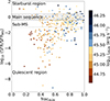 |
Fig. 8. Similar to Fig. 7, but with SFR/SFRMS as a function of fracAGN. Each point is colour-coded based on the CIGALE estimated log10LAGN. |
The detection of emission from star formation, while presenting apparent dust emission in the IR, matches the description of AGN2s found to be [NeV]λ3426 emitters (e.g. Vergani et al. 2018), known as composite systems with a combined contribution of star formation and AGNs to the electromagnetic spectrum, also presented in C2024. These results are also consistent with Hatcher et al. (2021), where AGN2s are typically found on or near the SF MS, and Ward et al. (2022), where cosmological simulations predict at 0 ≤ z ≤ 2 that AGNs are preferentially found in SF galaxies.
8. Comparison with AGN2 samples from the literature
In Vietri et al. (2022), optically selected AGN2s with redshifts between 0.5 and 0.9 from the VIMOS Public Extragalactic Redshift Survey(VIPERS) and VLT Deep Survey (VIMOS) surveys were studied to better understand the connection between AGN activity and the physical properties of the host galaxies. Similarly to this work, in Vietri et al. (2022) the CIGALE code was used to derive the stellar masses, while the SFR was computed using the [OII]λ3726+3728 doublet line. We compared our results to understand how the physical properties of our candidates are distributed. For stellar masses higher than 1010 M⊙, the majority of our sources are also below the MS.
The distribution of the Bongiorno sample and Vietri et al. (2022) on the SFR–M* diagram is very similar, with the majority of AGN2s clustered below the MS region and log10SFR ≤ 1.5. Both studies based their classification of AGNs on standard diagnostic diagrams [OIII]/Hβ versus [OII]/Hβ (see Rola et al. 1997; Lamareille 2010, and references therein). Therefore, their selection bias will provide sources with lower SFR as the majority of SF galaxies will be excluded from the sample5. Nevertheless, from Fig. 3, our selection provides us with a selection of sources with lower SFR than the aforementioned samples.
In this study, we constrain the photometry of our sample to preferentially select faint optical sources that align with the QSO2 sample from Alexandroff et al. (2013), as detailed in Sect. 2.1. This selection criterion will directly affect the estimated optical contribution to the SFR, enabling the IR contribution to be treated as a free parameter, that is, no constraints are applied to the IR data from WISE. Consequently, the results presented in Fig. 3 become particularly pertinent, as the optical contribution to the SFR estimation will be relatively minor compared to the IR contribution. Through our methodology, we identify QSO2 candidates across a broader range of SFRs, thus presenting a complex sample that potentially reflects different evolutionary mechanisms driving the observed properties.
9. Comparison with simulations: SPRITZ
We performed a comparison with the semi-empirical simulated SPRITZ catalogue6 (Bisigello et al. 2021a,b, 2022, master catalogue v1.131). In this catalogue, luminosity functions and galaxy populations are combined with SED simulated galaxies to reproduce physical properties, emission features, and expected fluxes using SED fitting for all simulated sources (see Bisigello et al. 2021b, and references therein). The galaxy populations are classified in SPRITZ based on the observations results presented in Gruppioni et al. (2013):
-
Non-AGN-dominated: SF galaxies with no clear AGN activity, which includes spiral and dwarf galaxies, SB galaxies, and passive elliptical galaxies with little or no star-formation.
-
AGNs: unobscured AGNs (AGN1s) and luminous galaxies with an AGN component dominating over the SF activity, with UV-optical obscuration due to dust (AGN2s).
-
Composite systems: SB-AGNs typically have highly obscured AGNs or are Compton-thick AGNs (NH ≥ 1023.5 cm−2) with a non-negligible component of star formation and enhanced MIR emission; SF-AGNs have properties similar to a spiral galaxy while having a low-luminosity or obscured AGN, with a ‘flattening’ in the 3–10 μm range. Furthermore, SF-AGNs (SB) and SF-AGNs (spiral) are divided based on their FIR and NIR colours and SED similarities.
For this work, we are particularly interested in the following subgroups within SPRITZ: AGN2, SB-AGN, and SF-AGN galaxies. These subgroups are expected to have similar properties as QSO2s, where dust obscuration plays a pivot role similarly to the SPRITZ subgroups, while having or not significant contribution from star-formation scenarios (e.g. Telesco et al. 1984; Farrah et al. 2003; Ivison et al. 2019; Jarvis et al. 2020, see also the references in our Sect. 7).
To ensure the SPRITZ simulated data represent the distribution in the SDSS survey, we set a constraint on the number density of galaxies. We limited the number of galaxies within each IR luminosity (i.e. LIR − z redshift) bin per square degree to match the SDSS observations. We set the following threshold: N * SDSS area > 1, where N represents the simulated galaxy count. This criterion ensures that only galaxies common enough to be observed at least once within the SDSS area are included in our analysis. We then apply the same magnitude criteria as described in Sect. 2. This step ensures the selection of optically faint sources, consistent with the selection criteria employed by both Alexandroff et al. (2013) and us. Finally, we imposed constraints on the physical properties of the simulated galaxies, log10(M*/M⊙) < 12 and log10(SFR [M⊙ yr−1]) < 3. These limits are based on established physical boundaries for galaxies and filter out objects with unrealistically high stellar masses or SFRs, which would create an unphysical bias.
In the SPRITZ catalogue, the physical properties were derived using the Multi-wavelength Analysis of Galaxy Physical Properties (MAGPHYS; da Cunha et al. 2012) code, or the SED3FIT (Berta et al. 2013), depending on the type of source and the presence of an AGN contribution. Although these codes differ from CIGALE, a comparison can be made to study the similarity between the simulated sources and our sample of QSO2 candidates.
In Fig. 9 we show the density plots for the LAGN, fracAGN, M*, SFR diagram for SF-AGNs, SB-AGNs, and AGN2s from SPRITZ alongside with our QSO2 candidates. The AGN sources selected from SPRITZ follow a similar distribution in the M*–SFR diagram as the QSO2 candidates within and above the MS, where the majority of candidates are placed. Although the estimates of physical properties used in SPRITZ and our work use different SED fitting codes, we observe a coherent range of physical properties between SPRITZ sources and our candidates.
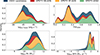 |
Fig. 9. Distribution plots of the fracAGN and LAGN for the QSO2 candidates (blue), SB-AGNs (red), SF-AGNs (orange), and AGN2s (green) from the SPRITZ catalogue. |
Considering these results, we can argue that the QSO2 sample comprises a mix of composite systems, with both SB and SF-AGN galaxies, and more ‘traditional’ AGN2 galaxies, whose host galaxy matches the properties of quiescent galaxies. To further study the true nature of our QSO2 sample, multi-wavelength analysis and morphological studies are necessary.
10. Conclusions
We have studied the physical properties of a sample of QSO2 candidates in the redshift desert (i.e. 1 ≤ z ≤ 2) selected via machine learning in C2024 (Cunha et al. 2024) using the SED fitting code CIGALE. Our aim was to obtain new insights into galaxy and AGN evolution across cosmic time.
We estimated relevant physical properties such as the SFR, M*, fracAGN, and AGN luminosity. Figure 3 illustrates the distribution of SDSS galaxies (used as a control sample, i.e. galaxies classified as non-QSO2 candidates in C2024), QSO2 candidates, and the Bongiorno sample (a subset from Bongiorno et al. 2012) on the SFR–M* diagram. While SDSS galaxies are primarily concentrated in the high-SFR region, the QSO2 candidates exhibit a broader distribution and include sources with lower SFRs. The QSO2 candidates also span a wide range of SFRs and high M* values, from 109 to 1012 M⊙ (see Fig. 4). We argue that our results demonstrate the ability of our methodology to identify QSO2 candidates independently of their host galaxy’s physical properties. This can be helpful in finding new AGN2 candidates and increasing our knowledge and statistics on this type of AGN.
Additionally, we computed the SFR/SFRMS parameter, which allowed us to classify our candidates into four areas: SB with log(SFR/SFRMS) > 0.4 dex; SF with log(SFR/SFRMS) ± 0.4 dex; sub-MS with log(SFR/SFRMS) between −0.4 and −1.3; and quiescent with log(SFR/SFRMS) < −1.3 (e.g. Aird et al. 2019; Vietri et al. 2022). Our candidates are distributed across the four regions, with higher concentrations in the quiescent and SF regions.
Sources in the quiescent region have high M*, significant fracAGN, and AGN luminosities that match the observed properties for AGN galaxies. The derived values for the AGN and host galaxy properties are consistent with those reported in the AGN literature (e.g. Hönig & Beckert 2007; Bongiorno et al. 2012; Vietri et al. 2022) and the Alexandroff sample (LAGN ∼ 1046.3 − 46.8 erg s−1; Alexandroff et al. 2013).
Speculating on their nature, we suggest that these sources may be subject to Compton-thick obscuration (NH ∼ 1024 cm−2), which would lead to an underestimation of the SFR due to the significant attenuation of optical light. Alternatively, they could be experiencing the effects of AGN feedback. Further observational data, spanning from imaging to spectroscopy, are necessary to unveil their nature and the co-evolution of the AGN and host galaxy, as well as to test these hypotheses. In particular, FIR data will be crucial to better constraining the physical properties derived in this study, especially SFRs and AGN luminosities.
We also compared our QSO2 candidate sample of composite systems (SB-AGNs and SF-AGNs) and AGN2 sources with the semi-empirical simulated catalogue SPRITZ. We observe a consistent distribution in the SFR–M* diagram when comparing the SPRITZ objects with our QSO2 candidates. This result provides compelling evidence of the effectiveness of our methodology in selecting a diverse population of obscured AGNs.
In conclusion, we have studied the physical properties of our sample of QSO2 candidates in the redshift desert using the available optical and IR photometry from SDSS and WISE. The estimated physical properties and consequent analysis herein showcase the relevance of novel methodologies for the identification of QSO2 galaxies, particularly in the less explored redshift regime. To further study the nature of QSO2 host galaxies, more multi-wavelength observations are essential (e.g. Zakamska et al. 2004, 2005; Ptak et al. 2006; Ramos Almeida et al. 2013). For example, imaging observations would enable morphological studies, which would help us study their merger history through disturbed morphologies or other distinctive features, testing the so-called merging paradigm (e.g. Zakamska et al. 2006; Villar-Martín et al. 2011; Bessiere et al. 2012; Ramos Almeida et al. 2012; Villar-Martín et al. 2012; Liu et al. 2013; Humphrey et al. 2015b,a, 2016; Pierce et al. 2023).
Data availability
The photometric data used were obtained through CasJobs7 and the SQL queries can be found here: https://github.com/pedro-acunha/AMELIA/tree/main/data. The machine learning code is available on GitHub: https://github.com/pedro-acunha/AMELIA. The derived physical properties of all candidates are available at the CDS via anonymous ftp to cdsarc.cds.unistra.fr (130.79.128.5) or via https://cdsarc.cds.unistra.fr/viz-bin/cat/J/A+A/696/A110
In Ji et al. (2022), the authors discuss a similar effect, where AGN selection methods for X-ray AGNs and IR AGNs show different physical properties for the AGN host galaxies.
Acknowledgments
PACC thanks the comments and suggestions from M. Villar-Martín, R. Carvajal, and I. Matute. PACC acknowledges financial support from Fundação para a Ciência e Tecnologia (FCT) through grant 2022.11477.BD, and through research grants UIDB/04434/2020 and UIDP/04434/2020. AH acknowledges support from NVIDIA through an NVIDIA Academic Hardware Grant Award. This publication uses data products from the Wide-field Infrared Survey Explorer, which is a joint project of the University of California, Los Angeles, and the Jet Propulsion Laboratory/California Institute of Technology, funded by the National Aeronautics and Space Administration. Funding for the Sloan Digital Sky Survey IV has been provided by the Alfred P. Sloan Foundation, the U.S. Department of Energy Office of Science, and the Participating Institutions. SDSS-IV acknowledges support and resources from the Center for High Performance Computing at the University of Utah. The SDSS website is www.sdss.org/. SDSS-IV is managed by the Astrophysical Research Consortium for the Participating Institutions of the SDSS Collaboration including the Brazilian Participation Group, the Carnegie Institution for Science, Carnegie Mellon University, Center for Astrophysics | Harvard & Smithsonian, the Chilean Participation Group, the French Participation Group, Instituto de Astrofísica de Canarias, The Johns Hopkins University, Kavli Institute for the Physics and Mathematics of the Universe (IPMU) / University of Tokyo, the Korean Participation Group, Lawrence Berkeley National Laboratory, Leibniz Institut für Astrophysik Potsdam (AIP), Max-Planck-Institut für Astronomie (MPIA Heidelberg), Max-Planck-Institut für Astrophysik (MPA Garching), Max-Planck-Institut für Extraterrestrische Physik (MPE), National Astronomical Observatories of China, New Mexico State University, New York University, University of Notre Dame, Observatário Nacional / MCTI, The Ohio State University, Pennsylvania State University, Shanghai Astronomical Observatory, United Kingdom Participation Group, Universidad Nacional Autónoma de México, University of Arizona, University of Colorado Boulder, University of Oxford, University of Portsmouth, University of Utah, University of Virginia, University of Washington, University of Wisconsin, Vanderbilt University, and Yale University. In preparation for this work, we used the following codes for Python: Numpy Harris et al. (2020), Scipy (Virtanen et al. 2020), Pandas (Wes et al. 2010), matplotlib (Hunter 2007), and seaborn (Waskom 2021).
References
- Abdurro’uf, Accetta, K., Aerts, C., et al. 2022, ApJS, 259, 35 [NASA ADS] [CrossRef] [Google Scholar]
- Ahumada, R., Prieto, C. A., Almeida, A., et al. 2020, ApJS, 249, 3 [Google Scholar]
- Aird, J., Coil, A. L., & Georgakakis, A. 2019, MNRAS, 484, 4360 [NASA ADS] [CrossRef] [Google Scholar]
- Alexander, D. M., & Hickox, R. C. 2012, New Astron. Rev., 56, 93 [Google Scholar]
- Alexander, D. M., Chary, R. R., Pope, A., et al. 2008, ApJ, 687, 835 [NASA ADS] [CrossRef] [Google Scholar]
- Alexandroff, R., Strauss, M. A., Greene, J. E., et al. 2013, MNRAS, 435, 3306 [NASA ADS] [CrossRef] [Google Scholar]
- Antonucci, R. 1993, ARA&A, 31, 473 [Google Scholar]
- Arnouts, S., & Ilbert, O. 2011, Astrophysics Source Code Library [record ascl:1108.009] [Google Scholar]
- Arnouts, S., Cristiani, S., Moscardini, L., et al. 1999, MNRAS, 310, 540 [Google Scholar]
- Aversa, R., Lapi, A., de Zotti, G., Shankar, F., & Danese, L. 2015, ApJ, 810, 74 [NASA ADS] [CrossRef] [Google Scholar]
- Azadi, M., Aird, J., Coil, A. L., et al. 2015, ApJ, 806, 187 [NASA ADS] [CrossRef] [Google Scholar]
- Bernhard, E., Mullaney, J. R., Daddi, E., Ciesla, L., & Schreiber, C. 2016, MNRAS, 460, 902 [NASA ADS] [CrossRef] [Google Scholar]
- Berta, S., Lutz, D., Santini, P., et al. 2013, A&A, 551, A100 [NASA ADS] [CrossRef] [EDP Sciences] [Google Scholar]
- Bessiere, P. S., Tadhunter, C. N., Ramos Almeida, C., & Villar Martín, M. 2012, MNRAS, 426, 276 [NASA ADS] [CrossRef] [Google Scholar]
- Bessiere, P. S., Tadhunter, C. N., Ramos Almeida, C., & Villar Martín, M. 2014, MNRAS, 438, 1839 [NASA ADS] [CrossRef] [Google Scholar]
- Bisigello, L., Caputi, K. I., Grogin, N., & Koekemoer, A. 2018, A&A, 609, A82 [NASA ADS] [CrossRef] [EDP Sciences] [Google Scholar]
- Bisigello, L., Gruppioni, C., Calura, F., et al. 2021a, PASA, 38, e064 [NASA ADS] [CrossRef] [Google Scholar]
- Bisigello, L., Gruppioni, C., Feltre, A., et al. 2021b, A&A, 651, A52 [NASA ADS] [CrossRef] [EDP Sciences] [Google Scholar]
- Bisigello, L., Vallini, L., Gruppioni, C., et al. 2022, A&A, 666, A193 [NASA ADS] [CrossRef] [EDP Sciences] [Google Scholar]
- Blain, A. W., Jameson, A., Smail, I., et al. 1999, MNRAS, 309, 715 [NASA ADS] [CrossRef] [Google Scholar]
- Blain, A. W., Barnard, V. E., & Chapman, S. C. 2003, MNRAS, 338, 733 [Google Scholar]
- Bolzonella, M., Miralles, J. M., & Pelló, R. 2000, A&A, 363, 476 [NASA ADS] [Google Scholar]
- Bongiorno, A., Merloni, A., Brusa, M., et al. 2012, MNRAS, 427, 3103 [Google Scholar]
- Boquien, M., Burgarella, D., Roehlly, Y., et al. 2019, A&A, 622, A103 [NASA ADS] [CrossRef] [EDP Sciences] [Google Scholar]
- Brandt, W. N., & Hasinger, G. 2005, ARA&A, 43, 827 [NASA ADS] [CrossRef] [Google Scholar]
- Brinchmann, J., & Ellis, R. S. 2000, ApJ, 536, L77 [NASA ADS] [CrossRef] [Google Scholar]
- Brinchmann, J., Charlot, S., White, S. D. M., et al. 2004, MNRAS, 351, 1151 [Google Scholar]
- Brusa, M., Fiore, F., Santini, P., et al. 2009, A&A, 507, 1277 [NASA ADS] [CrossRef] [EDP Sciences] [Google Scholar]
- Bruzual, G., & Charlot, S. 2003, MNRAS, 344, 1000 [NASA ADS] [CrossRef] [Google Scholar]
- Bugiani, L., Belli, S., Park, M., et al. 2025, ApJ, 981, 25 [NASA ADS] [CrossRef] [Google Scholar]
- Burgarella, D., Buat, V., & Iglesias-Páramo, J. 2005, MNRAS, 360, 1413 [NASA ADS] [CrossRef] [Google Scholar]
- Calzetti, D., Armus, L., Bohlin, R. C., et al. 2000, ApJ, 533, 682 [NASA ADS] [CrossRef] [Google Scholar]
- Carroll, C. M., Hickox, R. C., Masini, A., et al. 2021, ApJ, 908, 185 [NASA ADS] [CrossRef] [Google Scholar]
- Carroll, C. M., Ananna, T. T., Hickox, R. C., et al. 2023, ApJ, 950, 127 [NASA ADS] [CrossRef] [Google Scholar]
- Chabrier, G. 2003, PASP, 115, 763 [Google Scholar]
- Ciesla, L., Charmandaris, V., Georgakakis, A., et al. 2015, A&A, 576, A10 [NASA ADS] [CrossRef] [EDP Sciences] [Google Scholar]
- Comastri, A., Ranalli, P., Iwasawa, K., et al. 2011, A&A, 526, L9 [NASA ADS] [CrossRef] [EDP Sciences] [Google Scholar]
- Conroy, C. 2013, ARA&A, 51, 393 [NASA ADS] [CrossRef] [Google Scholar]
- Cresci, G., Mainieri, V., Brusa, M., et al. 2015, ApJ, 799, 82 [Google Scholar]
- Cunha, P. A. C., Humphrey, A., Brinchmann, J., et al. 2024, A&A, 687, A269 [NASA ADS] [CrossRef] [EDP Sciences] [Google Scholar]
- da Cunha, E., Charlot, S., Dunne, L., Smith, D., & Rowlands, K. 2012, in The Spectral Energy Distribution of Galaxies - SED 2011, eds. R. J. Tuffs & C. C. Popescu, 284, 292 [Google Scholar]
- Daddi, E., Alexander, D. M., Dickinson, M., et al. 2007, ApJ, 670, 173 [NASA ADS] [CrossRef] [Google Scholar]
- Dale, D. A., Helou, G., Magdis, G. E., et al. 2014, ApJ, 784, 83 [Google Scholar]
- Decarli, R., Falomo, R., Treves, A., et al. 2010, MNRAS, 402, 2453 [CrossRef] [Google Scholar]
- Di Matteo, T., Springel, V., & Hernquist, L. 2005, Nature, 433, 604 [NASA ADS] [CrossRef] [Google Scholar]
- Di Matteo, T., Colberg, J., Springel, V., Hernquist, L., & Sijacki, D. 2008, ApJ, 676, 33 [NASA ADS] [CrossRef] [Google Scholar]
- Donley, J. L., Koekemoer, A. M., Brusa, M., et al. 2012, ApJ, 748, 142 [Google Scholar]
- Fabian, A. C. 2012, ARA&A, 50, 455 [Google Scholar]
- Farrah, D., Afonso, J., Efstathiou, A., et al. 2003, MNRAS, 343, 585 [Google Scholar]
- Ferrarese, L., & Ford, H. 2005, Space Sci. Rev., 116, 523 [Google Scholar]
- Gaskell, C. M., Goosmann, R. W., Antonucci, R. R. J., & Whysong, D. H. 2004, ApJ, 616, 147 [NASA ADS] [CrossRef] [Google Scholar]
- Gebhardt, K., Kormendy, J., Ho, L. C., et al. 2000, ApJ, 543, L5 [CrossRef] [Google Scholar]
- Greene, J. E., & Ho, L. C. 2005, ApJ, 627, 721 [NASA ADS] [CrossRef] [Google Scholar]
- Greene, J. E., Zakamska, N. L., Ho, L. C., & Barth, A. J. 2011, ApJ, 732, 9 [NASA ADS] [CrossRef] [Google Scholar]
- Greenwell, C., Gandhi, P., Stern, D., et al. 2021, MNRAS, 503, L80 [NASA ADS] [CrossRef] [Google Scholar]
- Greenwell, C., Gandhi, P., Lansbury, G., et al. 2022, ApJ, 934, L34 [NASA ADS] [CrossRef] [Google Scholar]
- Gruppioni, C., Pozzi, F., Rodighiero, G., et al. 2013, MNRAS, 432, 23 [Google Scholar]
- Harris, C. R., Millman, K. J., van der Walt, S. J., et al. 2020, Nature, 585, 357 [NASA ADS] [CrossRef] [Google Scholar]
- Harrison, C. M., & Ramos Almeida, C. 2024, Galaxies, 12, 17 [NASA ADS] [CrossRef] [Google Scholar]
- Harrison, C. M., Costa, T., Tadhunter, C. N., et al. 2018, Nature Astronomy, 2, 198 [CrossRef] [Google Scholar]
- Hatcher, C., Kirkpatrick, A., Fornasini, F., et al. 2021, AJ, 162, 65 [NASA ADS] [CrossRef] [Google Scholar]
- Hatfield, P. W., Jarvis, M. J., Adams, N., et al. 2022, MNRAS, 513, 3719 [NASA ADS] [CrossRef] [Google Scholar]
- Hickox, R. C., & Alexander, D. M. 2018, ARA&A, 56, 625 [Google Scholar]
- Hickox, R. C., Jones, C., Forman, W. R., et al. 2007, ApJ, 671, 1365 [NASA ADS] [CrossRef] [Google Scholar]
- Hildebrandt, H., Arnouts, S., Capak, P., et al. 2010, A&A, 523, A31 [NASA ADS] [CrossRef] [EDP Sciences] [Google Scholar]
- Hinshaw, G., Larson, D., Komatsu, E., et al. 2013, ApJS, 208, 19 [Google Scholar]
- Hönig, S. F. 2019, ApJ, 884, 171 [Google Scholar]
- Hönig, S. F., & Beckert, T. 2007, MNRAS, 380, 1172 [CrossRef] [Google Scholar]
- Hopkins, P. F., Hernquist, L., Cox, T. J., et al. 2006, ApJS, 163, 1 [Google Scholar]
- Humphrey, A., Roche, N., Gomes, J. M., et al. 2015a, MNRAS, 447, 3322 [NASA ADS] [CrossRef] [Google Scholar]
- Humphrey, A., Villar-Martín, M., Ramos Almeida, C., et al. 2015b, MNRAS, 454, 4452 [Google Scholar]
- Humphrey, A., Villar-Martín, M., & Lagos, P. 2016, A&A, 585, A32 [NASA ADS] [CrossRef] [EDP Sciences] [Google Scholar]
- Hunter, J. D. 2007, Computing in Science& Engineering, 9, 90 [NASA ADS] [CrossRef] [Google Scholar]
- Ilbert, O., Arnouts, S., McCracken, H. J., et al. 2006, A&A, 457, 841 [NASA ADS] [CrossRef] [EDP Sciences] [Google Scholar]
- Ilbert, O., Capak, P., Salvato, M., et al. 2009, ApJ, 690, 1236 [NASA ADS] [CrossRef] [Google Scholar]
- Ivison, R. J., Page, M. J., Cirasuolo, M., et al. 2019, MNRAS, 489, 427 [NASA ADS] [CrossRef] [Google Scholar]
- Jarvis, M. E., Harrison, C. M., Mainieri, V., et al. 2020, MNRAS, 498, 1560 [NASA ADS] [CrossRef] [Google Scholar]
- Ji, Z., Giavalisco, M., Kirkpatrick, A., et al. 2022, ApJ, 925, 74 [NASA ADS] [CrossRef] [Google Scholar]
- Kewley, L. J., Geller, M. J., & Jansen, R. A. 2004, AJ, 127, 2002 [Google Scholar]
- Kormendy, J., & Ho, L. C. 2013, ARA&A, 51, 511 [Google Scholar]
- Lamareille, F. 2010, A&A, 509, A53 [CrossRef] [EDP Sciences] [Google Scholar]
- LaMassa, S. M., Civano, F., Brusa, M., et al. 2016, ApJ, 818, 88 [NASA ADS] [CrossRef] [Google Scholar]
- Lambrides, E. L., Chiaberge, M., Heckman, T., et al. 2020, ApJ, 897, 160 [Google Scholar]
- Lanzuisi, G., Delvecchio, I., Berta, S., et al. 2017, A&A, 602, A123 [NASA ADS] [CrossRef] [EDP Sciences] [Google Scholar]
- Leitherer, C., Calzetti, D., & Martins, L. P. 2002, ApJ, 574, 114 [NASA ADS] [CrossRef] [Google Scholar]
- Leja, J., Johnson, B. D., Conroy, C., & van Dokkum, P. 2018, ApJ, 854, 62 [NASA ADS] [CrossRef] [Google Scholar]
- Lilly, S. J., Le Fèvre, O., Renzini, A., et al. 2007, ApJS, 172, 70 [Google Scholar]
- Lin, D., Webb, N. A., & Barret, D. 2012, ApJ, 756, 27 [NASA ADS] [CrossRef] [Google Scholar]
- Liu, G., Zakamska, N. L., Greene, J. E., Nesvadba, N. P. H., & Liu, X. 2013, MNRAS, 430, 2327 [NASA ADS] [CrossRef] [Google Scholar]
- Liu, T., Tozzi, P., Wang, J.-X., et al. 2017, ApJS, 232, 8 [NASA ADS] [CrossRef] [Google Scholar]
- Lonsdale, C. J., Farrah, D., & Smith, H. E. 2006, in Astrophysics Update 2, ed. J. W. Mason, 285 [CrossRef] [Google Scholar]
- López, I. E., Brusa, M., Bonoli, S., et al. 2023, A&A, 672, A137 [NASA ADS] [CrossRef] [EDP Sciences] [Google Scholar]
- Lusso, E., Comastri, A., Vignali, C., et al. 2011, A&A, 534, A110 [NASA ADS] [CrossRef] [EDP Sciences] [Google Scholar]
- Lynden-Bell, D. 1969, Nature, 223, 690 [NASA ADS] [CrossRef] [Google Scholar]
- Madau, P., & Dickinson, M. 2014, ARA&A, 52, 415 [Google Scholar]
- Magorrian, J., Tremaine, S., Richstone, D., et al. 1998, AJ, 115, 2285 [Google Scholar]
- Mainieri, V., & Cosmos Collaboration 2009, in Chandra’s First Decade of Discovery, eds. S. Wolk, A. Fruscione, & D. Swartz, 147 [Google Scholar]
- Małek, K., Buat, V., Roehlly, Y., et al. 2018, A&A, 620, A50 [Google Scholar]
- Marton, G., Gezer, I., Madarász, M., et al. 2024, A&A, 688, A203 [NASA ADS] [CrossRef] [EDP Sciences] [Google Scholar]
- Merritt, D., & Ferrarese, L. 2001a, MNRAS, 320, L30 [NASA ADS] [CrossRef] [Google Scholar]
- Merritt, D., & Ferrarese, L. 2001b, ApJ, 547, 140 [NASA ADS] [CrossRef] [Google Scholar]
- Noeske, K. G., Weiner, B. J., Faber, S. M., et al. 2007, ApJ, 660, L43 [CrossRef] [Google Scholar]
- Noll, S., Burgarella, D., Giovannoli, E., et al. 2009, A&A, 507, 1793 [NASA ADS] [CrossRef] [EDP Sciences] [Google Scholar]
- Pacifici, C., Iyer, K. G., Mobasher, B., et al. 2023, ApJ, 944, 141 [NASA ADS] [CrossRef] [Google Scholar]
- Padovani, P., Alexander, D. M., Assef, R. J., et al. 2017, A&ARv, 25, 2 [Google Scholar]
- Paulino-Afonso, A., González-Gaitán, S., Galbany, L., et al. 2022, A&A, 662, A86 [NASA ADS] [CrossRef] [EDP Sciences] [Google Scholar]
- Pickles, A. J. 1998, PASP, 110, 863 [NASA ADS] [CrossRef] [Google Scholar]
- Pierce, J. C. S., Tadhunter, C., Ramos Almeida, C., et al. 2023, MNRAS, 522, 1736 [NASA ADS] [CrossRef] [Google Scholar]
- Polletta, M., Tajer, M., Maraschi, L., et al. 2007, ApJ, 663, 81 [NASA ADS] [CrossRef] [Google Scholar]
- Ptak, A., Zakamska, N. L., Strauss, M. A., et al. 2006, ApJ, 637, 147 [NASA ADS] [CrossRef] [Google Scholar]
- Ramos Almeida, C., Bessiere, P. S., Tadhunter, C. N., et al. 2012, MNRAS, 419, 687 [NASA ADS] [CrossRef] [Google Scholar]
- Ramos Almeida, C., Bessiere, P. S., Tadhunter, C. N., et al. 2013, MNRAS, 436, 997 [NASA ADS] [CrossRef] [Google Scholar]
- Richstone, D., Ajhar, E. A., Bender, R., et al. 1998, Nature, 385, A14 [Google Scholar]
- Rigopoulou, D., Mainieri, V., Almaini, O., et al. 2009, MNRAS, 400, 1199 [NASA ADS] [CrossRef] [Google Scholar]
- Rodríguez, M. I., Villar-Martín, M., Emonts, B., et al. 2014, A&A, 565, A19 [NASA ADS] [CrossRef] [EDP Sciences] [Google Scholar]
- Rola, C. S., Terlevich, E., & Terlevich, R. J. 1997, MNRAS, 289, 419 [NASA ADS] [Google Scholar]
- Ross, N., Strauss, M. A., Greene, J. E., et al. 2014, American Astronomical Society Meeting Abstracts, 223, 115.04 [NASA ADS] [Google Scholar]
- Salvato, M., Hasinger, G., Ilbert, O., et al. 2009, ApJ, 690, 1250 [CrossRef] [Google Scholar]
- Sanders, D. B., & Mirabel, I. F. 1996, ARA&A, 34, 749 [Google Scholar]
- Sanders, D. B., Soifer, B. T., Elias, J. H., et al. 1988, ApJ, 325, 74 [Google Scholar]
- Schreiber, C., Pannella, M., Elbaz, D., et al. 2015, A&A, 575, A74 [NASA ADS] [CrossRef] [EDP Sciences] [Google Scholar]
- Seyfert, C. K. 1943, ApJ, 97, 28 [NASA ADS] [CrossRef] [Google Scholar]
- Shimwell, T. W., Hardcastle, M. J., Tasse, C., et al. 2022, A&A, 659, A1 [NASA ADS] [CrossRef] [EDP Sciences] [Google Scholar]
- Sokol, A. D., Yun, M., Pope, A., Kirkpatrick, A., & Cooke, K. 2023, MNRAS, 521, 818 [NASA ADS] [CrossRef] [Google Scholar]
- Stalevski, M., Fritz, J., Baes, M., & Popovic, L. C. 2012, in Torus Workshop 2012, eds. R. Mason, A. Alonso-Herrero, & C. Packham, 170 [Google Scholar]
- Stalevski, M., Ricci, C., Ueda, Y., et al. 2016, MNRAS, 458, 2288 [Google Scholar]
- Stalevski, M., González-Gaitán, S., Savić, D., et al. 2023, MNRAS, 519, 3237 [NASA ADS] [CrossRef] [Google Scholar]
- Sturm, E., Hasinger, G., Lehmann, I., et al. 2006, ApJ, 642, 81 [NASA ADS] [CrossRef] [Google Scholar]
- Symeonidis, M., Kartaltepe, J., Salvato, M., et al. 2013, MNRAS, 433, 1015 [NASA ADS] [CrossRef] [Google Scholar]
- Telesco, C. M., Becklin, E. E., Wynn-Williams, C. G., & Harper, D. A. 1984, ApJ, 282, 427 [NASA ADS] [CrossRef] [Google Scholar]
- Thorne, J. E., Robotham, A. S. G., Davies, L. J. M., et al. 2022, MNRAS, 509, 4940 [Google Scholar]
- Treister, E., & Urry, C. M. 2012, Advances in Astronomy, 2012, 516193 [Google Scholar]
- Urry, C. M., & Padovani, P. 1995, PASP, 107, 803 [NASA ADS] [CrossRef] [Google Scholar]
- Vergani, D., Garilli, B., Polletta, M., et al. 2018, A&A, 620, A193 [NASA ADS] [CrossRef] [EDP Sciences] [Google Scholar]
- Vietri, G., Garilli, B., Polletta, M., et al. 2022, A&A, 659, A129 [NASA ADS] [CrossRef] [EDP Sciences] [Google Scholar]
- Villar-Martín, M., Tadhunter, C., Humphrey, A., et al. 2011, MNRAS, 416, 262 [NASA ADS] [Google Scholar]
- Villar-Martín, M., Cabrera Lavers, A., Bessiere, P., et al. 2012, MNRAS, 423, 80 [CrossRef] [Google Scholar]
- Villar Martín, M., Perna, M., Humphrey, A., et al. 2020, A&A, 634, A116 [NASA ADS] [CrossRef] [EDP Sciences] [Google Scholar]
- Villar Martín, M., Emonts, B. H. C., Cabrera Lavers, A., et al. 2021, A&A, 650, A84 [CrossRef] [EDP Sciences] [Google Scholar]
- Violino, G., Stevens, J., & Coppin, K. 2016, in Active Galactic Nuclei 12: A Multi-Messenger. Perspective, AGN12, 68 [Google Scholar]
- Virtanen, P., Gommers, R., Oliphant, T. E., et al. 2020, Nature Methods, 17, 261 [CrossRef] [Google Scholar]
- Ward, S. R., Harrison, C. M., Costa, T., & Mainieri, V. 2022, MNRAS, 514, 2936 [NASA ADS] [CrossRef] [Google Scholar]
- Waskom, M. L. 2021, Journal of Open Source Software, 6, 3021 [CrossRef] [Google Scholar]
- Wes, M. 2010, in Proceedings of the 9th Python in Science Conference, eds. S. van der Walt, & J. Millman, 56 [Google Scholar]
- Wright, E. L., Eisenhardt, P. R. M., Mainzer, A. K., et al. 2010, AJ, 140, 1868 [Google Scholar]
- Xue, Y. Q., Luo, B., Brandt, W. N., et al. 2011, ApJS, 195, 10 [Google Scholar]
- Yan, W., Brandt, W. N., Zou, F., et al. 2023, ApJ, 951, 27 [NASA ADS] [CrossRef] [Google Scholar]
- Yang, G., Boquien, M., Buat, V., et al. 2020, MNRAS, 491, 740 [Google Scholar]
- Yang, G., Boquien, M., Brandt, W. N., et al. 2022, ApJ, 927, 192 [NASA ADS] [CrossRef] [Google Scholar]
- Yuan, S., Strauss, M. A., & Zakamska, N. L. 2016, MNRAS, 462, 1603 [NASA ADS] [CrossRef] [Google Scholar]
- Zakamska, N. L., Strauss, M. A., Krolik, J. H., et al. 2003, AJ, 126, 2125 [NASA ADS] [CrossRef] [Google Scholar]
- Zakamska, N. L., Strauss, M. A., Heckman, T. M., Ivezić, Ž., & Krolik, J. H. 2004, AJ, 128, 1002 [NASA ADS] [CrossRef] [Google Scholar]
- Zakamska, N. L., Schmidt, G. D., Smith, P. S., et al. 2005, AJ, 129, 1212 [NASA ADS] [CrossRef] [Google Scholar]
- Zakamska, N. L., Strauss, M. A., Krolik, J. H., et al. 2006, AJ, 132, 1496 [NASA ADS] [CrossRef] [Google Scholar]
Appendix A: SED fitting parameters
CIGALE SED fitting parameters used for the control sample (galaxies).
CIGALE SED fitting parameters used for the QSO2 candidates.
Appendix B: LePhare++ photo-z estimations
We present examples of photometric redshift estimation using LePhare++. By fitting templates to observed flux densities from SDSS and WISE, we classify sources based on the reduced χ2 value, as shown in Fig. B.1. The fitting process includes galaxy, QSO, and star templates, highlighting the challenges LePhare++ faces with composite systems. In such cases, the optical portion of the SED often aligns closely with the galaxy template, while the IR portion is dominated by the QSO template. These examples show the limitations of current templates in accurately modelling optical-obscured AGNs.
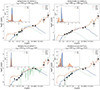 |
Fig. B.1. Examples of the best-fitting models for photometric redshift estimation using LePhare++ for four sources. Filled symbols represent the observed flux densities from SDSS and WISE. Source classification is defined by the reduced χ2 value. The best-fit galaxy template is shown in blue, the best-fit QSO template in orange, and the best-fit star template in green. The histograms within each plot show the probability distribution function for the photometric redshift estimation, with the vertical dashed line indicating the spectroscopic redshift from SDSS. |
Appendix C: CIGALE fitting examples
In this section we present four example fits generated with CIGALE, corresponding to the same candidates shown in Appendix B. Each plot illustrates the contributions of various components to the overall SED of each candidate – the attenuated stellar emission, unattenuated stellar emission, nebular emission, dust emission, and AGN emission – as well as the complete model spectrum, which combines all components. These examples show how more complex models, such as SKIRTOR, are needed to model the AGN contribution to the SED of our candidates. For comparison purposes, we show in Table C.1 the physical properties derived for the sources shown in Fig. C.1.
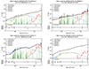 |
Fig. C.1. Best-fitting models for four candidates using CIGALE, similar to Fig. B.1. Open symbols represent observed flux densities, and the red-filled symbols indicate modelled flux densities. The goodness of fit is shown by the reduced χ2 value, with the residuals of the fit displayed at the bottom of each panel. The derived physical properties are listed in Table C.1. |
Physical properties derived using CIGALE for the four sources shown in Figs. B.1 and C.1.
Appendix D: SED mock comparison
To understand whether the estimated physical properties using CIGALE, with SDSS and WISE photometry, we used the mock catalogue option provided in the CIGALE configuration file.
The mock catalogue is built, for each source, using the best fit and introducing random errors to each quantity from a Gaussian distribution with the same standard deviation as the observation uncertainty. In Fig. D.1, we show the linear correlation between the mock and predicted values.
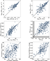 |
Fig. D.1. Comparison between the estimated physical properties as derived from the mock analysis and the values estimated using CIGALE. The dashed grey line indicates the 1:1 relation between the parameters. From top to bottom, left to right: SFR; stellar mass; AGN luminosity; AGN fraction; viewing angle (inclination); and polar-dust extinction, E(B-V). |
All Tables
Statistical metrics for the photo-z derived using LePhare++, compared with SDSS spectroscopic redshifts, when considering QSO and galaxies templates.
Physical properties derived using CIGALE for the four sources shown in Figs. B.1 and C.1.
All Figures
|
Fig. 1. Stacked spectrum of QSO2 candidates with normalised median flux in the rest-frame wavelength, obtained through spline interpolation using available SDSS spectra. The spectrum is additionally normalised based on the number of contributing spectra for each rest-frame wavelength. Grey vertical lines mark the positions of emission lines in the rest frame. The plot includes two zoomed-in regions: (1) 3326–3526 Å, highlighting the [NeV]λ3426 emission line, and (2) 3630–3830 Å, highlighting the [OII]λλ3727, 3730 emission lines. The red line represents the Gaussian fit applied to the spectrum. |
| In the text | |
|
Fig. 2. 2D histogram of the stellar mass, M* (top) and specific AGN luminosity, LAGN/M*, defined in Thorne et al. (2022, bottom), as a function of fracAGN for the QSO2 sample. The colour gradient indicates the density of sources for each bin. The median and standard deviation are represented by the solid and dashed orange lines, respectively. The vertical black line indicates the fracAGN > 0.1 threshold used in Leja et al. (2018) to characterise sources with significant AGN contribution. |
| In the text | |
|
Fig. 3. SFR as a function of stellar mass (M*) for the QSO2 candidates (black dots) on a logarithmic scale. The star formation MS described by Schreiber et al. (2015) at the mean SDSS spectroscopic redshift of our candidates (z = 1.1) is shown as a solid line, with dashed lines indicating a 0.4 dex deviation. The contours display the M*–SFR distribution for X-ray and optically selected AGN2s from the zCOSMOS survey by Bongiorno et al. (2012) with redshifts 1 ≤ z ≤ 2 (orange) and for the control sample of SDSS galaxies (blue). |
| In the text | |
|
Fig. 4. Difference between the estimated SFR and the MS SFR for the QSO2 candidates, the control sample, the Bongiorno sample (Bongiorno et al. 2012), and the Zakamska sample (Zakamska et al. 2003). The solid grey line represents the MS of star formation found by Schreiber et al. (2015) at z = 1.1, and the dashed lines give a scatter of ±0.4 dex. |
| In the text | |
|
Fig. 5. Comparison between physical properties estimated with and without radio LoTSS photometry, using CIGALE. Left: scatter plots comparing the properties of galaxies with and without radio LoTSS photometry, such as the AGN fraction, AGN luminosity, stellar mass, and SFR. All values are provided in logarithmic scale, with the exception of the fracAGN. Each scatter plot includes a 1:1 reference line, as a dashed red line. Right: bar plots of the differences in the same properties, for each source (numbered in the x axis): SDSS+WISE – SDSS+WISE+LoTSS. |
| In the text | |
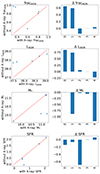 |
Fig. 6. Same as Fig. 5 but for XMM-Newton photometry. |
| In the text | |
|
Fig. 7. Measurements of the logarithm of the ratio SFR/SFRMS as a function of the logarithm of stellar mass, M*. The SFRs relative to the MS of star formation for galaxies were computed assuming the average redshift from our QSO2 candidate sample, z = 1.1, and using the relation from Schreiber et al. (2015). The dashed line separates the MS and the SB region at 0.4 dex, as defined by Aird et al. (2019). The blue-shaded area defines the MS region. Each point is colour-coded based on the estimated AGN fraction of CIGALE, fracAGN. |
| In the text | |
|
Fig. 8. Similar to Fig. 7, but with SFR/SFRMS as a function of fracAGN. Each point is colour-coded based on the CIGALE estimated log10LAGN. |
| In the text | |
|
Fig. 9. Distribution plots of the fracAGN and LAGN for the QSO2 candidates (blue), SB-AGNs (red), SF-AGNs (orange), and AGN2s (green) from the SPRITZ catalogue. |
| In the text | |
|
Fig. B.1. Examples of the best-fitting models for photometric redshift estimation using LePhare++ for four sources. Filled symbols represent the observed flux densities from SDSS and WISE. Source classification is defined by the reduced χ2 value. The best-fit galaxy template is shown in blue, the best-fit QSO template in orange, and the best-fit star template in green. The histograms within each plot show the probability distribution function for the photometric redshift estimation, with the vertical dashed line indicating the spectroscopic redshift from SDSS. |
| In the text | |
|
Fig. C.1. Best-fitting models for four candidates using CIGALE, similar to Fig. B.1. Open symbols represent observed flux densities, and the red-filled symbols indicate modelled flux densities. The goodness of fit is shown by the reduced χ2 value, with the residuals of the fit displayed at the bottom of each panel. The derived physical properties are listed in Table C.1. |
| In the text | |
|
Fig. D.1. Comparison between the estimated physical properties as derived from the mock analysis and the values estimated using CIGALE. The dashed grey line indicates the 1:1 relation between the parameters. From top to bottom, left to right: SFR; stellar mass; AGN luminosity; AGN fraction; viewing angle (inclination); and polar-dust extinction, E(B-V). |
| In the text | |
Current usage metrics show cumulative count of Article Views (full-text article views including HTML views, PDF and ePub downloads, according to the available data) and Abstracts Views on Vision4Press platform.
Data correspond to usage on the plateform after 2015. The current usage metrics is available 48-96 hours after online publication and is updated daily on week days.
Initial download of the metrics may take a while.