| Issue |
A&A
Volume 688, August 2024
|
|
|---|---|---|
| Article Number | A79 | |
| Number of page(s) | 10 | |
| Section | Extragalactic astronomy | |
| DOI | https://doi.org/10.1051/0004-6361/202449601 | |
| Published online | 06 August 2024 | |
AGN populations in the local Universe: Their alignment with the main sequence, stellar population characteristics, accretion efficiency, and the impact of AGN feedback
1
Instituto de Fisica de Cantabria (CSIC-Universidad de Cantabria), Avenida de los Castros, 39005 Santander, Spain
e-mail: This email address is being protected from spambots. You need JavaScript enabled to view it.
2
National Observatory of Athens, Institute for Astronomy, Astrophysics, Space Applications and Remote Sensing, Ioannou Metaxa and Vasileos Pavlou, 15236 Athens, Greece
Received:
13
February
2024
Accepted:
16
May
2024
Abstract
In this study, we used a sample of 338 galaxies – within the redshift range of 0.02 < z < 0.1 drawn from the Sloan Digital Sky Survey (SDSS) – for which there are available classifications based on their emission line ratios. We identified and selected Compton-thick (CT) AGN through the use of X-ray and infrared luminosities at 12 μm. We constructed the spectral energy distributions (SEDs) for all sources and fit them using the CIGALE code to derive properties related to both the AGN and host galaxies. Employing stringent criteria to ensure the reliability of SED measurements, our final sample comprises 14 CT AGN, 118 Seyfert 2 (Sy2), 82 composite, and 124 low-ionization nuclear emission-line regions (LINER) galaxies. Our analysis reveals that, irrespective of their classification, the majority of the sources lie below the star-forming main sequence (MS). Additionally, a lower level of AGN activity is associated with a closer positioning to the MS. Using the Dn4000 spectral index as a proxy for the age of stellar populations, we observe that, compared to other AGN classes, LINERs exhibit the oldest stellar populations. Conversely, CT sources are situated in galaxies with the youngest stellar populations. Furthermore, LINER and composite galaxies tend to show the lowest accretion efficiency, while CT AGN, on average, display the most efficient accretion among the four AGN populations. Our findings are consistent with a scenario in which the different AGN populations might not originate from the same AGN activity burst. Early triggers in gas-rich environments can create high-accretion-rate supermassive black holes (SMBHs), leading to a progression from CT to Sy2, while later triggers in gas-poor stages result in low-accretion-rate SMBHs like those found in LINERs.
Key words: methods: observational / galaxies: active / galaxies: evolution / galaxies: Seyfert
© The Authors 2024
 Open Access article, published by EDP Sciences, under the terms of the Creative Commons Attribution License (https://creativecommons.org/licenses/by/4.0), which permits unrestricted use, distribution, and reproduction in any medium, provided the original work is properly cited.
This article is published in open access under the Subscribe to Open model. This email address is being protected from spambots. You need JavaScript enabled to view it. to support open access publication.
1. Introduction
In the realm of active galactic nuclei (AGN), the local Universe presents a diverse population of galaxies hosting different AGN classes, each characterized by distinct observational features. Among these classes, there are low-ionization nuclear emission-line regions (LINERs), Seyferts, and composite galaxies that consist of both AGN and star-forming systems, each offering valuable insights into the intricate interplay between supermassive black holes (SMBHs) and their host galaxies. Understanding the properties and behaviors of these AGN classes is crucial in order to unravel the mechanisms that drive their activity and influence the evolution of their host systems.
Investigating the star formation rate (SFR) and stellar mass, M*, of galaxies hosting AGN provides a crucial contextual framework for comprehending their evolutionary trajectories (e.g., Rosario et al. 2012, 2013; Santini et al. 2012; Mullaney et al. 2015; Masoura et al. 2018; Bernhard et al. 2019; Mountrichas et al. 2021a,b, 2023, 2024a; Koutoulidis et al. 2022; Pouliasis et al. 2022; Mountrichas & Buat 2023). These parameters offer essential clues about the ongoing astrophysical processes within these galaxies, shedding light on the co-evolution of AGN and their host galaxies. LINERs, Seyferts, and composite galaxies, serve as unique laboratories with which to explore the interdependencies between AGN activity, star formation, and the overall stellar content of their host systems.
The study of stellar populations across the different AGN populations offers a glimpse into the historical star formation activity within these systems (e.g., Kauffmann et al. 2003a,b; Kewley et al. 2006; Mountrichas et al. 2022a; Georgantopoulos et al. 2023). Utilizing parameters such as the Dn4000 spectral index, which serves as a proxy for the age of stellar populations, enables researchers to unravel the past evolutionary paths of these galaxies.
The Eddington ratio, denoted nEdd, emerges as a pivotal parameter in quantifying the accretion efficiency of AGN. Defined as the ratio of the bolometric luminosity to the Eddington luminosity (i.e., the maximum luminosity an AGN can emit; LEdd = 1.26 × 1038 MBH/M⊙ erg s−1, where MBH is the mass of the SMBH), nEdd provides insights into the balance between radiation pressure and gravitational forces around the SMBH. Examining the nEdd values for different AGN populations allows for a comparative analysis of their accretion processes, offering a deeper understanding of the diverse ways in which AGN interact with their environments (e.g., Kewley et al. 2006; Georgantopoulos et al. 2023; Mountrichas & Georgantopoulos 2024; Mountrichas et al. 2024b).
Previous studies have found that LINER galaxies tend to have higher M*, redder optical colors and higher black hole masses compared to Seyferts (e.g. Smolčić 2009). LINERs also are more dusty and more concentrated than Seyferts, although, these differences could be, mainly, due to the different nEdd of the AGN populations, with LINERs to be dominant at low nEdd and Seyferts dominant at high nEdd (e.g., Kewley et al. 2006). Seyferts also appear to reside in dark matter holes with lower mass compared to LINERs (Constantin & Vogeley 2006). For an in-depth overview of the various AGN populations, refer to Heckman & Best (2014).
Previous studies found that LINER galaxies tend to have higher M*, redder optical colors, and higher black hole masses compared to Seyferts (e.g., Smolčić 2009). LINERs are also more dusty and more concentrated than Seyferts, although these differences could mainly be due to the different nEdd of the AGN populations, with LINERs being dominant at low nEdd and Seyferts dominant at high nEdd (e.g., Kewley et al. 2006). Seyferts also appear to reside in dark matter holes with lower mass compared to LINERs (Constantin & Vogeley 2006). For an in-depth overview of the various AGN populations, refer to Heckman & Best (2014).
In this work, we used galaxies from the Sloan Digital Sky Survey (SDSS; Almeida et al. 2023) for which classifications are available based on their emission lines. Specifically, sources are categorized into Seyfert 2 (Sy2), composite, and LINER galaxies. Furthermore, we identified and selected CT AGN using their X-ray and infrared luminosities at 12 μm. The data and the CT selection criteria are described in Sect. 2. In Sect. 3, we describe the process followed to fit the spectral energy distributions (SEDs) of all the sources using the CIGALE code, as well as the strict selection criteria we applied to select galaxies with robust SED fitting measurements. We performed a comprehensive investigation of SFR, M*, accretion efficiency, and stellar populations to decipher the intricate connections between AGN activity and the broader processes governing galaxy evolution in the local Universe. We present our results in Sect. 4. and discuss our main findings and compare them with prior studies in Sect. 5. Finally, in Sect. 6 we present a summary of our main findings.
2. Data
2.1. Sample selection
Our goal is to select a sample of obscured, low-redshift AGN observed in X-rays, while minimizing the contamination of star-forming galaxies. To this end, we followed the criteria presented in Zhang (2023) for selecting type 2 AGN in the SDSS: we selected all objects in the SDSS-DR18 (Almeida et al. 2023) spectroscopic database (specObj table) classified as galaxies and given the subclass AGN by the SDSS pipeline. We restricted our sample to galaxies with redshift below 0.1. In order to exclude local galaxies with a large extension, where the SDSS photometry is highly unreliable, we imposed an additional redshift cut of z > 0.02 (with this limit, the spectrograph fiber covers ≳1 kpc of the nuclear region). We also selected only objects with a good quality spectrum, that is, with a median signal-to-noise ratio (S/N) of higher than 10 and no warnings in the estimated redshift. Finally, we kept only objects with a primary entry in the photometric database of SDSS and included in the Portsmouth catalog of stellar kinematics and emission-line flux measurements (Thomas et al. 2013). This catalog models the SDSS spectrum to derive the emission line properties and gives a reliable spectral classification (Seyfert, LINER, composite, etc.) based on BPT diagrams for each galaxy.
The final query that reflects this selection is:
SELECT * FROM specObj AS sp
JOIN PhotoObj AS ph
 ON sp.bestObjID=ph.objID
JOIN emissionLinesPort AS ln
 ON sp.specObjID=ln.specObjID
WHERE
 sp.class=`galaxy' AND sp.subclass=`AGN'
 AND (sp.z BETWEEN 0.02 AND 0.1)
 AND sp.zwarning=0 AND sp.snmedian>10
This query returns a total of 7382 sources in the SDSS-DR18 database. In order to select sources observed in X-rays, we queried the position of each galaxy in the RapidXMM database (Ruiz et al. 2022). This system provides X-ray flux upper limits for all positions in the sky that have been observed by XMM-Newton. As of May 20231, we found 479 objects from our initial sample of 7382 galaxies in fields observed by XMM-Newton. Of these 479 sources, 210 have a counterpart within 5 arcsec in the 4XMM-DR13 catalog (Webb et al. 2020). The 4XMM-DR13 catalog was built using XMM-Newton observations released up to 2022 December 31. Our sample contains sources in 22 observations that were not included in the 4XMM-DR13. For these cases, we used the X-ray source catalogs generated by the XMM-Newton pipeline available in the archive, finding six additional sources with X-ray counterparts. In total, about 45 per cent (216 sources out of 479 sources) of our final sample is detected in X-rays.
2.2. Photometry
In order to perform the SED analysis described in Sect. 3.1, we need to build SEDs with good photometric coverage. In the ultraviolet (UV), we search for counterparts in the Revised Catalog for the GALEX All-Sky Imaging Survey (GALEX-AIS, Bianchi et al. 2017). In the mid-infrared (MIR) regime, we used the AllWISE catalog (Cutri et al. 2013). For the near-infrared (NIR) photometry, we relied on three catalogs: Most of our sources have counterparts in the 2MASS Extended Source Catalog (2MASS-XSC, Skrutskie et al. 2006). When no counterpart was found in the 2MASS-XSC, we used the UKIDSS-DR11plus Large Area survey catalog (UKIDSS-LAS, Lawrence 2007) if that sky region was covered by this survey; otherwise, we searched for a counterpart in the 2MASS Point Source Catalog (2MASS-PSC, Skrutskie et al. 2006).
Given the low redshift of our selected sample, most of our sources are extended sources clearly resolved in the optical and NIR bands. In order to correctly estimate galaxy properties, we need to select measurements of the magnitudes that recover the emission of the whole galaxy. We used Petrosian magnitudes for the five SDSS bands (u, g, r, i, z), as recommended for photometry of nearby galaxies. We used the “best” FUV and NUV GALEX magnitudes, as recommended in the AIS catalog documentation. For sources with 2MASS-XSC photometry, we used the isophotal J, H and K magnitudes. In the case of UKIDSS-LAS, we used the Petrosian magnitudes for the J, H, and K bands. In AllWISE, we used the elliptical aperture magnitudes for the four WISE bands (W1, W2, W3, and W4) when available; otherwise, we used the profile-fitting magnitudes. We visually inspected the images in the different bands and the constructed SEDs to check that the different apertures used for measuring the magnitudes covered the same region of the galaxy.
3. Analysis
3.1. Galaxy properties
To compute the properties of AGN and their host galaxies (e.g., AGN bolometric luminosity, SFR, M*), we employed SED fitting through the CIGALE algorithm (Boquien et al. 2019; Yang et al. 2020, 2022). We adhered to the same templates and parametric grid in the SED fitting process as those used in prior works (e.g., Koutoulidis et al. 2022; Mountrichas et al. 2022b). In summary, we modeled the galaxy component using a delayed star-formation history (SFH) model with a functional form of SFR ∝ t × exp(−t/τ). We incorporated a continuous star-formation period of 50 Myr as a star-formation burst (Małek et al. 2018; Buat et al. 2019). We modeled stellar emission using the single stellar population templates of Bruzual & Charlot (2003), attenuated in accordance with the Charlot & Fall (2000) attenuation law. To model nebular emission, CIGALE adopts nebular templates based on Villa-Velez et al. (2021). The emission from dust heated by stars is modeled following Dale et al. (2014), excluding any AGN contribution. The AGN emission is included using the SKIRTOR models of Stalevski et al. (2012, 2016). The parameter space employed in the SED fitting process is presented in Table 1.
Models and the values for their free parameters used by X-CIGALE for the SED fitting of our galaxy sample.
3.2. Reliability criteria
To ensure the reliability of our analysis, we implement selection criteria akin to those employed in prior studies (e.g., Mountrichas et al. 2022a,c; Buat et al. 2021; Pouliasis et al. 2022; Mountrichas & Buat 2023). Specifically, in order to exclude sources with unreliable SED fitting measurements and host galaxy information, we set a reduced χ2 threshold of  (e.g., Masoura et al. 2018; Buat et al. 2021). This criterion led to the exclusion of six sources from our dataset. Additionally, we omit systems for which the CIGALE algorithm cannot constrain the SFR and M*. For this purpose, we leveraged the two values provided by CIGALE for each estimated galaxy property. One value corresponds to the best model, while the other (Bayes) represents the likelihood-weighted mean value. A substantial disparity between these two calculations implies a complex likelihood distribution and significant uncertainties. Consequently, we only incorporated sources in our analysis that satisfy the conditions
  and
and  , where SFRbest and M*, best are the best-fit values of SFR and M*, respectively, and SFRbayes and M*, bayes are the Bayesian values estimated by CIGALE.
There are 338 sources that meet the specified criteria. Among these sources, we identified and selected 14 CT AGN candidates (see following section). From the remaining 324 galaxies, 118 are classified as Sy2, 82 as composite, and 124 as LINER galaxies based on the Portsmouth catalog (Thomas et al. 2013). These are the sources used in our analysis (Table 2).
Number of sources included within each AGN population considered in our analysis.
3.3. Selection of Compton-thick AGN candidates
One of the goals of this work is to identify potential CT AGNs and study the properties of their host galaxy in comparison with the overall properties of the type 2 AGN population. CT AGN show X-ray absorption with hydrogen column densities of NH > 1024 cm−2 that largely suppress the direct X-ray emission below 10 keV (Ricci et al. 2015; Georgantopoulos & Akylas 2019; Torres-Albà et al. 2021).
In order to identify CT candidates, we followed the work of Pfeifle et al. (2022), who present a diagnostic for the X-ray absorption in AGN based on the ratio of the MIR to the 2–10 keV X-ray luminosities. As the MIR luminosity represents a reliable proxy for the isotropic AGN emission, a low X-ray-to-MIR-luminosity ratio is a strong indication of a CT source (Alexander et al. 2008; Georgantopoulos et al. 2011; Rovilos et al. 2014). Pfeifle et al. (2022) use the BAT AGN Spectroscopic Survey (BASS Koss et al. 2017, 2022; Ricci et al. 2017a; Ichikawa et al. 2017), which includes sources detected in the ultrahard X-ray band (14–195 keV) and is expected to be a complete census of the most luminous AGN in the local Universe and to be independent of X-ray obscuration.
Using the same data set and methods of Pfeifle et al. (2022), we estimated the expected completeness and purity levels for CT samples using different X-ray-to-12-μm luminosity ratios, as shown in Fig. 1. Our results show that for log(Lobs(2 − 10 keV)/L(12 μm)) < −1.6 we can expect ∼80% completeness with a purity of ∼80%.
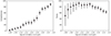 |
Fig. 1. Completeness (left) and purity (right) for CT AGN in the BASS sample depending on different selection criteria based on the X-ray-to-MIR luminosity ratio. |
We estimated the X-ray-to-12-μm luminosity ratios for our sample of low-z type 2 AGNs. As this is a spectroscopically selected sample of nearby objects, it includes objects with low-luminosity AGNs and the host galaxy emission dominates even in the MIR range. Hence, in order to avoid contamination due to the host galaxy, the 12 μm luminosity we used for estimating the Pfeifle et al. (2022) diagnostic is that corresponding to the AGN emission we obtained in our SED analysis using CIGALE (see Sect. 3.1).
According to the Pfeifle et al. (2022) diagnostic discussed above, we considered CT candidates to be those sources below the log(Lobs(2 − 10 keV)/L(12 μm)) = −1.6 line and optically classified as Sy2 galaxies (see Fig. 2). We found a total of 14 CT candidates. Our CT sample is by no means complete. This is because we discarded sources with low-quality optical spectra, namely those with S/N < 10. Some CT sources – especially the fainter ones – may be among the discarded sources. In addition, our selected log(Lobs(2 − 10 keV)/L(12 μm)) < −1.6 criterion can find only 80% of the known CT AGN, while among the selected CT AGN, only 80% are bona fide CT AGN. Finally, the low log(Lobs(2 − 10 keV)/L(12 μm)) ratio criterion may be sensitive to other types of sources such as turnoff AGN; see for example the discussion in Saade et al. (2022).
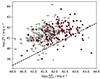 |
Fig. 2. AGN luminosity at 12 μm as estimated by CIGALE versus observed X-ray luminosity in the 2–10 keV band for our sample of local SDSS AGN. Gray circles correspond to LINER+Composite objects, and red circles are Seyfert 2 galaxies. Symbols marked with a horizontal and/or vertical bar show upper limits in the 12 μm and/or X-ray luminosity, respectively. The black, dashed line shows |
Next we checked the literature to see whether or not our sources with reasonably good-quality X-ray observations available are indeed associated with CT AGN. Of our 14 sources, 3 have been observed by NuSTAR: NGC 5765, IC2227, and LEDA 1373882. Masini et al. (2019) find that NGC 5765 is a reflection-dominated CT AGN with NH ∼ 1025 cm−2. NuSTAR observations of IC 2227 were reported by Silver et al. (2022). These authors find that the source is heavily obscured with NH ∼ 3 × 1023 cm−2. The remaining source has not been detected by NuSTAR. Next, we searched for additional information in the literature regarding the X-ray spectra of the remaining 11 sources. The vast majority of these are faint sources, with fluxes below 5 × 10⁻¹⁴ erg cm−2 s−1, thus impeding the extraction of good-quality spectra. One of our candidate sources (LEDA1593164) has not been detected and there is only an upper limit in X-ray flux available (see e.g., Ruiz et al. 2021). Three of our sources are associated with targets: NGC 5765, IC 2227, and 2MASSX1390454+5603528. In Table 3 we give the full list of our CT candidate sources.
Candidate Compton-thick sources.
4. Results
In this section, we present an exploration of the location of diverse AGN populations in relation to the star-forming main sequence (MS) and show how we investigated the influence of SMBH activity on this location. Additionally, we conducted a comparison of their stellar populations and analyzed the accretion power exhibited by our sources.
4.1. The position of the AGN classes relative to the main sequence
To examine the relative positioning of the different AGN populations in relation to the star-forming MS, we first investigated the distribution of our selected galaxies in the SFR–M* plane (Sect. 4.1.1) and then compared the SFR of the sources in our dataset to the SFR of star-forming MS galaxies as a function of luminosity (Sect. 4.1.2).
4.1.1. Distribution of sources in the SFR–M* plane
In Fig. 3, we illustrate the distribution of the AGN populations in the SFR–M* plane. Additionally, we incorporate the local SFR–M* relation as determined from SDSS galaxies by Elbaz et al. (2007), which is represented by the gray line for reference. Notably, the majority of our sources appear below this line, indicating that our sources predominantly inhabit quiescent systems. Table 4 provides median values and their corresponding 25th and 75th percentiles for each host galaxy property and AGN class. Intriguingly, LINER galaxies exhibit the highest M* (by ∼0.2 dex) and the lowest SFR compared to other AGN classes. Among the four AGN classes, CT sources display the highest median SFR values. Despite these disparities, we note that Kolmogorov–Smirnov (KS) tests indicate that these differences lack statistical significance (i.e., < 2σ), as the p-values obtained range from 0.2 to 0.9 (where a p-value = 0.05 signifies a statistical significance of ∼2σ). Similar outcomes are observed with other statistical tests, such as Mann–Whitney, Anderson, and Kuiper tests.
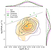 |
Fig. 3. Distribution of sources in the SFR–M* plane. Different AGN populations are presented with different colors and lines, as indicated in the legend of the plot. The solid gray line shows the local SFR–M* relation presented in Elbaz et al. (2007) for SDSS galaxies. |
Median values and their 25th and 75th percentiles for the SFR, M*, sSFR, Dn4000, Hδ, and λsBHAR of the different AGN populations examined in our study.
Figure 4 depicts the distributions of sSFR ( ) for different AGN classes, with median values and their corresponding 25th and 75th percentiles provided in Table 4. LINER galaxies exhibit the lowest sSFR compared to other AGN populations, which display comparable median values and sSFR distributions, with the exception of CT AGN, which display the highest median sSFR values. Notably, despite the fact that the p-values obtained from the comparison of the LINER sSFR distribution with that of other AGN populations are relatively low (ranging from 0.1 to 0.2) compared to those from the comparison of SFR and M* distributions, the differences are not statistically significant at a 2σ level.
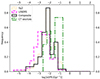 |
Fig. 4. Distribution of sSFR ( |

4.1.2. SFRnorm versus luminosity
An alternative way to illustrate the position of AGN relative to the MS is to calculate the SFRnorm parameter (e.g., Mullaney et al. 2015; Masoura et al. 2018, 2021; Bernhard et al. 2019; Koutoulidis et al. 2022; Pouliasis et al. 2022; Mountrichas et al. 2022c, 2023; Mountrichas & Buat 2023). SFRnorm is defined as the ratio of the SFR of AGN to the SFR of star-forming MS galaxies with comparable M* and redshift. Therefore, SFRnorm > 1 indicates that the AGN is located above the MS, whereas SFRnorm < 1 indicates that the AGN is below the MS. For the calculation of SFRnorm, we used the expression derived in Elbaz et al. (2007), who used SDSS galaxies in the local Universe. It is important to note that using analytical expressions from existing literature for estimating SFRnorm may introduce systematic biases, as opposed to employing galaxy control samples (Mountrichas et al. 2021b). However, for the purposes of our analysis, these potential systematic uncertainties do not impact our results or conclusions.
Figure 5 presents the distribution of our sources in the SFR space. LSF and LAGN are the luminosities originating from star formation and the AGN, respectively. Both parameters are defined as the integrated luminosities in the range between 8 and 1000 μm. To gauge the accuracy of the CIGALE estimations for these parameters, we can check how well CIGALE calculates the AGN fraction, fracAGN, because it is defined as the fraction of the total IR emission coming from the AGN and therefore is derived from data within similar wavelengths to LSF and LAGN. Figure 6 presents the distributions of fracAGN for the four AGN populations. This plot demonstrates the considerable range of AGN activity present in our sources. Sy2 and CT appear to have the highest fracAGN values (median values of 0.28 and 0.44, respectively) compared to composite and LINER galaxies (median values of 0.14 and 0.17, respectively).
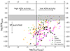 |
Fig. 5. SFRnorm as a function of the ratio of the star-formation luminosity (LSF) to the AGN luminosity (LAGN). SFRnorm is defined as the ratio of the SFR of the AGN to the SFR calculated using the Elbaz et al. (2007) expression for SDSS galaxies. The gray shaded area indicates an area of ±0.3 dex around log SFRnorm = 0 to denote the main sequence. Below the gray area, the star formation of the AGN host galaxies is quenched. The dashed vertical lines indicates the |


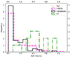 |
Fig. 6. Distributions of the AGN fractions calculated by CIGALE for the different AGN populations, as indicated in the legend. The AGN fraction is defined as the fraction of the total IR emission coming from the AGN. |
To evaluate the accuracy of fracAGN, we used mock catalogs generated by CIGALE based on the best-fitting model for each source in our dataset. CIGALE essentially creates a mock sample by taking the best-fitting flux for each source and introducing noise to it, which is derived from a Gaussian distribution with the same standard deviation as the observed flux. The mock data are then analyzed in the same manner as the actual observations. The precision of each estimated parameter can be assessed by comparing the original input values to the output values from the analysis (ground truth versus estimated value).
Our investigation reveals that the difference between the original and estimated values of the AGN fractions has a mean value of 0.05 (median value of 0.02), with a dispersion of 0.16. When we focus on sources with low AGN fractions (less than 0.2), the mean difference is 0.04 (median difference is 0.03), with a dispersion of 0.08. Given these findings, we consider the calculated AGN fractions, and by extension the calculated luminosities originating from star formation (LSF) and AGN (LAGN), to be reliable.
Having addressed the reliability of the LSF and LAGN parameters, we now examine the distribution of our sources in the SFR space (Fig. 5). In systems that have
  (or < 0 in logarithmic space), the AGN activity dominates over star-formation activity, while
  implies either a more starburst-dominated galaxy or relatively low AGN luminosities (Netzer 2009). The gray shaded area indicates a ±0.3 dex around the MS (i.e., around SFRnorm = 1). We note that, regardless of the AGN class, in all cases SFRnorm increases with
  , signifying that the AGN host galaxy is closer to the MS for higher values of
  . This trend could stem from either an elevation in LSF, a reduction in LAGN, or a combination of both factors as galaxies approach the MS. To identify the primary contributor of what drives the AGN toward or away from the MS, we computed the slopes of the SFR–M* relation for various AGN populations (see Fig. 3) using the linmix module (Kelly 2007). Linmix conducts a linear regression between two parameters by iteratively adjusting the data points within their uncertainties. The findings indicate that the slope gradually flattens as we transition from CT (slope of 1.24), to Sy2 (0.78), to composite (0.59), and ultimately to LINER galaxies (0.51). Therefore, AGN populations with higher AGN activity (based on their AGN fraction measurements, i.e., CT and Sy2) appear to have steeper slopes compared to AGN systems with lower AGN activity (i.e., composite and LINER galaxies). This may suggest that the AGN activity is aiding in quenching the SFR in the examined systems.
Overall, our analysis indicates that the majority of the sources examined in this study are positioned below the MS. LINERs preferentially inhabit galaxies characterized by higher stellar mass and lower levels of SFR activity compared to Sy2, composite, and CT sources. However, these distinctions do not reach statistical significance exceeding 2σ. We also find indications that CT sources may present enhanced levels of star formation compared to non-CT AGN. Additionally, our results suggest that a lower level of AGN activity corresponds to a closer positioning of the host galaxy to the MS.
4.2. The stellar populations of the different AGN classes
We subsequently conducted a comparative analysis of the stellar populations among galaxies hosting different AGN classes. In Fig. 7, we illustrate the distributions of the various AGN populations in the Hδ–Dn4000 space. Recognizing that more massive systems tend to harbor older stars, we applied weights to these distributions based on the M* of the sources. Specifically, we assigned a weight to each AGN to match the M* of the four AGN classes (e.g., Mountrichas et al. 2022a). It is important to highlight that, while the Dn4000 measurements exhibit relatively small uncertainties (with a median uncertainty value of approximately 10% of the measured value), the uncertainties associated with Hδ are notably larger (with a median value of Hδ uncertainties of around 80% of the measured value). Consequently, while we provide the distributions of the Hδ spectral line, our primary conclusions are derived from the results based on the Dn4000 spectral index due to its comparatively small errors.
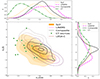 |
Fig. 7. Distribution of the different AGN populations in the Hδ–Dn4000 space. We also plot the results for the heavily obscured (NH > 1023 cm−2) AGN sample used in Georgantopoulos et al. (2023), at z ∼ 1 (LEGA-C, brown, dotted contours). |
Our findings indicate that LINER galaxies exhibit, on average, the oldest stellar populations compared to the other AGN classes. Sy2 and composite galaxies display stars of similar age, while CT sources showcase the youngest stars among the various AGN classes examined in our study. Although the statistical tests do not reveal significant differences based on the calculated p-values, likely due to the broad distributions, the observed patterns in the distributions are notably distinct. The median values along with their corresponding 25th and 75th percentiles for each galaxy population are presented in Table 4.
These findings align with the outcomes presented in the previous section. Specifically, LINER galaxies, which are characterized by the lowest star-formation activity among the various AGN classes, demonstrate the highest Dn4000 values, indicating they harbor the oldest stellar populations. Composite and Sy2 galaxies, which share similar levels of star-formation activity, also tend to possess comparable stellar populations. Furthermore, these results are consistent with those in the previous section, underscoring that CT sources, on average, display heightened star-formation activity and host the youngest stellar populations among the AGN classes examined in this study.
In Fig. 7, we also juxtapose the distribution of our sources in the Hδ–Dn4000 space with that of the heavily obscured LEGA-C AGN, as presented in Georgantopoulos et al. (2023; illustrated by brown dotted contours). In the study by Georgantopoulos et al. (2023), 73 AGN in the COSMOS field were examined, with available measurements for their spectral indices obtained from the LEGA-C catalog (van der Wel et al. 2021) at redshifts within 0.6 < z < 1. This latter investigation involved a comparison of various properties, including M*, sSFR, Eddington ratio, and stellar populations between heavily obscured and nonobscured AGN using X-ray criteria for the classification of the sources and applying a threshold at NH = 1023 cm−2. Notably, the LEGA-C AGN exhibit lower Dn4000 values (and higher Hδ values) compared to our sample. It is crucial to acknowledge that the two AGN populations differ not only in terms of their redshifts but also in their classification criteria, their M* properties (see bottom panel of Fig. 4), and LX (LEGA-C AGN are about two orders of magnitude more luminous compared to the sources used in our analysis; see also the discussion in Sect. 5).
4.3. The accretion efficiency of different AGN classes
In this section, we show how we investigated the accretion efficiency across various AGN classes within our datasets. This efficiency is measured through the nEdd. In cases where the MBH measurements are not available, the specific black hole accretion rate, λsBHAR, is used as a proxy for nEdd (e.g., Aird et al. 2018; Mountrichas et al. 2021b, 2022b). For the calculation of λsBHAR, the following expression is used:
 (1)
(1)
To calculate λsBHAR, we employed the measurements of Lbol and M* provided by CIGALE. It is important to acknowledge that the effectiveness of λsBHAR as a proxy for nEdd hinges on factors such as the scatter in the MBH − M* relation and the accuracy of AGN bolometric luminosity estimates, as previous studies have shown (Lopez et al. 2023; Mountrichas & Buat 2023). Nonetheless, in our examination, we emphasize the comparison of λsBHAR across distinct AGN classes rather than its absolute values.
Figure 8 displays the distributions of λsBHAR for various AGN populations in our dataset (top panel). The corresponding median values and percentiles are shown in Table 4. Our findings indicate that LINER and composite galaxies exhibit analogous λsBHAR distributions and median values, which are also the lowest among the AGN classes considered. Sy2 galaxies tend to exhibit higher λsBHAR values, while CT sources present the highest λsBHAR values within the AGN populations in our sample. The KS-test indicates that these distinctions hold statistical significance at a level exceeding > 2σ, as the p-values range from 10−5 to 10−7. Comparable p-values are obtained through other statistical tests, including Mann–Whitney, Anderson, and Kuiper.
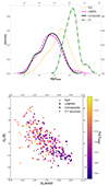 |
Fig. 8. Specific black hole accretion rate, λsBHAR, for the different AGN populations. The top panel shows the distribution of λsBHAR for the different AGN classes. The bottom panel shows the distribution of our sources in the Hδ–Dn4000 space, which are color coded based on their λsBHAR values. |
The bottom panel of Fig. 8 presents the distribution of the different AGN classes in the Hδ–Dn4000 space, color-coded based on the λsBHAR of the sources. The results indicate that sources with younger stellar populations (i.e., Dn4000 < 1.4) tend to exhibit higher λsBHAR values compared to sources with older stars. This is in line with the findings of Georgantopoulos et al. (2023, see their Fig. 4).
5. Discussion
In this work, we identified CT sources and investigated their properties as a different AGN class, comparing them with the other AGN populations. We find indications that CT sources may present enhanced levels of star-formation activity, but most importantly our analysis reveals that CT sources are hosted by galaxies that have the youngest stellar population and their SMBHs present the highest accretion efficiency across the different AGN classes. Georgantopoulos et al. (2023) used AGN in the COSMOS field and found that highly obscured sources (NH > 1023 cm−2) live in galaxies with older stars (higher Dn4000 values) compared to their unobscured (or moderately obscured) counterparts. Their analysis also showed that highly obscured AGN have lower nEdd compared to unobscured sources.
However, it is important to note that our sample is significantly different from that used in Georgantopoulos et al. (2023) in several respects. In Georgantopoulos et al. (2023), the classification of sources is based on X-ray criteria, as opposed to the optically classified sources employed in our work. Previous works have shown that the two classification schemes do not necessarily coincide (e.g., Merloni et al. 2014; Li et al. 2019; Masoura et al. 2020). Furthermore, our dataset spans significantly lower X-ray luminosities (the majority of our sources have log[LX,2#x2212;10 keV (erg s−1)] < 42) compared to the luminosities probed by the COSMOS sample that is used in Georgantopoulos et al. (2023), where 42.5 < log[LX,2#x2212;10 keV (erg s−1)] < 44.3. Moreover, the galaxies employed in the Georgantopoulos et al. (2023) analysis are more massive than our galaxies, with a median difference of ∼0.7 dex. Therefore, apart from the redshift difference between the two datasets, it is likely that the two studies probe different AGN populations, which may have been triggered by different physical processes. Previous studies also suggest that the SFRs of (X-ray or optically selected) obscured and unobscured AGN differ as a function of redshift and LX (e.g., Mountrichas & Georgantopoulos 2024; Mountrichas et al. 2024a,b).
Our results also show higher λsBHAR values for Sy2 galaxies compared to composite and LINER galaxies. Previous studies found that type 1 AGN exhibit elevated λsBHAR values in comparison to type 2 AGN (e.g., Mountrichas & Georgantopoulos 2024). Similar outcomes have been observed when the AGN classification is based on X-ray criteria (e.g., Ricci et al. 2017b, 2022, 2023; Georgantopoulos et al. 2023; Mountrichas et al. 2024b). The higher λsBHAR values of unobscured type 1 AGN compared to obscured type 2 AGN has been attributed to the effect of radiation pressure. Specifically, at higher Eddington ratios, radiation pressure may lead to a reduction in the covering factor of obscuring gas, making observations of unobscured sources more likely than observations of obscured ones (Ricci et al. 2017b). Our analysis also incorporates CT sources, which exhibit the highest λsBHAR values among the four AGN classes examined in this study. In Fig. 3 and the extended data in Fig. 1 of Ricci et al. (2017a), there is a suggestion of elevated λsBHAR values for CT sources compared to Compton-thin AGN (NH = 1022 − 24 cm−2). High λsBHAR values for CT AGN were also reported by Brightman et al. (2016) (log λsBHAR ∼ −1) based on 12 megamaser AGN detected by NuSTAR.
Leslie et al. (2016) employed data from the SDSS data release 7 in their study, analyzing properties calculated by the MPA/JHU group. It is worth noting that their methods for computing host galaxy properties differ from our SED fitting analysis. Their investigation revealed that composite, Seyfert, and LINER galaxies are positioned below the main sequence, emphasizing the substantial impact of AGN activity in suppressing star formation in these systems. Moreover, based on their findings, LINERs have, on average, the lowest SFR and the highest M* among the different AGN populations. Our results align remarkably well with their observations.
In an investigation conducted by Kewley et al. (2006), the authors focused on 85 224 emission-line galaxies selected from SDSS and identified a significant distinction between Seyferts and LINERs, particularly in terms of their nEdd. Their analysis indicated that LINERs tend to exhibit predominantly lower nEdd values compared to Sy2 galaxies. Our results align with these observations. Additionally, their investigation into the stellar populations of different AGN classes, based on the distributions of the D4000 spectral index, revealed that LINER galaxies have older stellar populations (higher D4000 values) compared to Seyferts. Once again, our findings are consistent with these outcomes.
Our results could indicate that the different types of AGN examined here may result from distinct phases of AGN activity. For example, if a SMBH becomes active early in a galaxy’s evolution, when there is plenty of gas, it might exhibit a high accretion rate, appearing as a Sy2 and potentially transitioning from CT to Sy2. On the other hand, if the AGN activity begins later in the galaxy’s history when gas is less abundant, the SMBH would likely have a lower accretion rate, leading to a LINER (e.g., Torres-Papaqui et al. 2024).
6. Conclusions
In this work, we used 338 galaxies at 0.02 < z < 0.1 to study the AGN and host galaxy properties of different (nonquasar) AGN classes included in the SDSS-DR18 catalog. Classifications are available for these sources based on their emission-line ratios. Specifically, galaxies are classified into Sy2, composite, and LINER. Among these sources, we identified and selected CT AGN using their LX–L12 μm relation (Asmus et al. 2014) and applying the threshold suggested by Pfeifle et al. (2022). We constructed and fitted the SED of the sources using the CIGALE code and applied strict criteria to include only sources with reliable SED fitting measurements in our analysis. Our sample consists of 118 Sy2, 82 composite, 124 LINER, and 14 CT sources. The 14 CT AGN are classified as Sy2 and were excluded from the Sy2 population here. These sources have available measurements for their Dn4000 and Hδ spectral indices, which serve as proxies for their stellar populations. Our goal is to examine the positions of these AGN populations relative to the main sequence, and compare their stellar populations and their accretion efficiency. Our main findings are summarized as follows:
-
The majority of sources, regardless of their classification, are situated below the main sequence. LINERs predominantly reside in galaxies characterized by higher stellar mass and lower levels of star formation activity compared to Sy2, composite, and CT sources.
-
Our findings suggest that a lower level of AGN activity corresponds to a closer alignment of the host galaxy with the main sequence.
-
When comparing their spectral indices, LINERs exhibit the oldest stellar populations (indicated by higher Dn4000 values) of all the AGN populations studied here. Composite and Sy2 galaxies show stellar populations of similar age, while CT AGN host the youngest stellar populations among the classes examined in this study.
-
In LINER and composite galaxies, the AGN display the lowest accretion efficiency (lower specific black hole accretion values), while CT AGN, on average, exhibit the most efficient accretion among the four AGN populations.
In summary, our comprehensive analysis sheds light on the diverse characteristics of AGN host galaxies, emphasizing the intricate interplay between AGN activity, stellar populations, and accretion efficiency. These insights contribute to a deeper understanding of the multifaceted nature of AGN and their impact on host galaxy properties.
XMM-Newton observations are ingested into the RapidXMM system when the data become public, and so queries at a later date can give a larger number.
Acknowledgments
This project has received funding from the European Union’s Horizon 2020 research and innovation program under grant agreement no. 101004168, the XMM2ATHENA project.
References
- Aird, J., Coil, A. L., & Georgakakis, A. 2018, MNRAS, 474, 1225 [NASA ADS] [CrossRef] [Google Scholar]
- Alexander, D. M., Chary, R. R., Pope, A., et al. 2008, ApJ, 687, 835 [NASA ADS] [CrossRef] [Google Scholar]
- Almeida, A., Anderson, S. F., Argudo-Fernández, M., et al. 2023, ApJS, 267, 44 [NASA ADS] [CrossRef] [Google Scholar]
- Asmus, D., Hönig, S. F., Gandhi, P., Smette, A., & Duschl, W. J. 2014, MNRAS, 439, 1648 [NASA ADS] [CrossRef] [Google Scholar]
- Bernhard, E., Grimmett, L. P., Mullaney, J. R., et al. 2019, MNRAS, 483, L52 [NASA ADS] [CrossRef] [Google Scholar]
- Bianchi, L., Shiao, B., & Thilker, D. 2017, ApJS, 230, 24 [Google Scholar]
- Boquien, M., Burgarella, D., Roehlly, Y., et al. 2019, A&A, 622, A103 [NASA ADS] [CrossRef] [EDP Sciences] [Google Scholar]
- Brightman, M., Masini, A., Ballantyne, D. R., et al. 2016, ApJ, 826, 93 [NASA ADS] [CrossRef] [Google Scholar]
- Bruzual, G., & Charlot, S. 2003, MNRAS, 344, 1000 [NASA ADS] [CrossRef] [Google Scholar]
- Buat, V., Ciesla, L., Boquien, M., Małek, K., & Burgarella, D. 2019, A&A, 632, A79 [NASA ADS] [CrossRef] [EDP Sciences] [Google Scholar]
- Buat, V., Mountrichas, G., Yang, G., et al. 2021, A&A, 654, A93 [NASA ADS] [CrossRef] [EDP Sciences] [Google Scholar]
- Charlot, S., & Fall, S. M. 2000, ApJ, 539, 718 [Google Scholar]
- Constantin, A., & Vogeley, M. S. 2006, ApJ, 650, 727 [NASA ADS] [CrossRef] [Google Scholar]
- Cutri, R. M., Wright, E. L., Conrow, T., et al. 2013, Explanatory Supplement to the AllWISE Data Release Products [Google Scholar]
- Dale, D. A., Helou, G., Magdis, G. E., et al. 2014, ApJ, 784, 83 [Google Scholar]
- Elbaz, D., Daddi, E., Borgne, D. L., et al. 2007, A&A, 468, 33 [NASA ADS] [CrossRef] [EDP Sciences] [Google Scholar]
- Georgantopoulos, I., & Akylas, A. 2019, A&A, 621, A28 [NASA ADS] [CrossRef] [EDP Sciences] [Google Scholar]
- Georgantopoulos, I., Rovilos, E., Akylas, A., et al. 2011, A&A, 534, A23 [NASA ADS] [CrossRef] [EDP Sciences] [Google Scholar]
- Georgantopoulos, I., Pouliasis, E., Mountrichas, G., et al. 2023, A&A, 673, A67 [NASA ADS] [CrossRef] [EDP Sciences] [Google Scholar]
- Heckman, T. M., & Best, P. N. 2014, ARA&A, 52, 589 [Google Scholar]
- Ichikawa, K., Ricci, C., Ueda, Y., et al. 2017, ApJ, 835, 74 [NASA ADS] [CrossRef] [Google Scholar]
- Kauffmann, G., Heckman, T. M., White, S. D. M., et al. 2003a, MNRAS, 341, 54 [Google Scholar]
- Kauffmann, G., Heckman, T. M., White, S. D. M., et al. 2003b, MNRAS, 341, 33 [Google Scholar]
- Kelly, B. C. 2007, ApJ, 665, 1489 [Google Scholar]
- Kewley, L. J., Groves, B., Kauffmann, G., & Heckman, T. 2006, MNRAS, 372, 961 [Google Scholar]
- Koss, M., Trakhtenbrot, B., Ricci, C., et al. 2017, ApJ, 850, 74 [Google Scholar]
- Koss, M. J., Ricci, C., Trakhtenbrot, B., et al. 2022, ApJS, 261, 2 [NASA ADS] [CrossRef] [Google Scholar]
- Koutoulidis, L., Mountrichas, G., Georgantopoulos, I., Pouliasis, E., & Plionis, M. 2022, A&A, 658, A35 [NASA ADS] [CrossRef] [EDP Sciences] [Google Scholar]
- Lawrence, A., Warren, S. J., Almaini, O., et al. 2007, MNRAS, 379, 1599 [Google Scholar]
- Leslie, S. K., Kewley, L. J., Sanders, D. B., & Lee, N. 2016, MNRAS, 455, L82 [NASA ADS] [CrossRef] [Google Scholar]
- Li, J., Xue, Y., Sun, M., et al. 2019, ApJ, 877, 5 [NASA ADS] [CrossRef] [Google Scholar]
- Lopez, I. E., Brusa, M., Bonoli, S., et al. 2023, A&A, 672, A137 [NASA ADS] [CrossRef] [EDP Sciences] [Google Scholar]
- Małek, K., Buat, V., Roehlly, Y., et al. 2018, A&A, 620, A50 [Google Scholar]
- Masini, A., Comastri, A., Hickox, R. C., et al. 2019, ApJ, 882, 83 [Google Scholar]
- Masoura, V. A., Mountrichas, G., Georgantopoulos, I., et al. 2018, A&A, 618, A31 [NASA ADS] [CrossRef] [EDP Sciences] [Google Scholar]
- Masoura, V. A., Georgantopoulos, I., Mountrichas, G., et al. 2020, A&A, 638, A45 [NASA ADS] [CrossRef] [EDP Sciences] [Google Scholar]
- Masoura, V. A., Mountrichas, G., Georgantopoulos, I., & Plionis, M. 2021, A&A, 646, A167 [EDP Sciences] [Google Scholar]
- Merloni, A., Bongiorno, A., Brusa, M., et al. 2014, MNRAS, 437, 3550 [Google Scholar]
- Mountrichas, G., & Buat, V. 2023, A&A, 679, A151 [NASA ADS] [CrossRef] [EDP Sciences] [Google Scholar]
- Mountrichas, G., & Georgantopoulos, I. 2024, A&A, 683, A160 [NASA ADS] [CrossRef] [EDP Sciences] [Google Scholar]
- Mountrichas, G., Buat, V., Georgantopoulos, I., et al. 2021a, A&A, 653, A70 [NASA ADS] [CrossRef] [EDP Sciences] [Google Scholar]
- Mountrichas, G., Buat, V., Yang, G., et al. 2021b, A&A, 653, A74 [NASA ADS] [CrossRef] [EDP Sciences] [Google Scholar]
- Mountrichas, G., Buat, V., Yang, G., et al. 2022a, A&A, 667, A145 [NASA ADS] [CrossRef] [EDP Sciences] [Google Scholar]
- Mountrichas, G., Masoura, V. A., Xilouris, E. M., et al. 2022b, A&A, 661, A108 [NASA ADS] [CrossRef] [EDP Sciences] [Google Scholar]
- Mountrichas, G., Buat, V., Yang, G., et al. 2022c, A&A, 663, A130 [NASA ADS] [CrossRef] [EDP Sciences] [Google Scholar]
- Mountrichas, G., Yang, G., Buat, V., et al. 2023, A&A, 675, A137 [NASA ADS] [CrossRef] [EDP Sciences] [Google Scholar]
- Mountrichas, G., Masoura, V. A., Corral, A., & Carrera, F. J. 2024a, A&A, 683, A143 [NASA ADS] [CrossRef] [EDP Sciences] [Google Scholar]
- Mountrichas, G., Viitanen, A., Carrera, F. J., et al. 2024b, A&A, 683, A172 [NASA ADS] [CrossRef] [EDP Sciences] [Google Scholar]
- Mullaney, J. R., Alexander, D. M., Aird, J., et al. 2015, MNRAS, 453, L83 [Google Scholar]
- Netzer, H. 2009, MNRAS, 399, 1907 [CrossRef] [Google Scholar]
- Pfeifle, R. W., Ricci, C., Boorman, P. G., et al. 2022, ApJS, 261, 3 [NASA ADS] [CrossRef] [Google Scholar]
- Pouliasis, E., Mountrichas, G., Georgantopoulos, I., et al. 2022, A&A, 667, A56 [NASA ADS] [CrossRef] [EDP Sciences] [Google Scholar]
- Ricci, C., Ueda, Y., Koss, M. J., et al. 2015, ApJ, 815, L13 [Google Scholar]
- Ricci, C., Trakhtenbrot, B., Koss, M. J., et al. 2017a, ApJS, 233, 17 [Google Scholar]
- Ricci, C., Trakhtenbrot, B., Koss, M. J., et al. 2017b, Nature, 549, 488 [NASA ADS] [CrossRef] [Google Scholar]
- Ricci, C., Ananna, T. T., Temple, M. J., et al. 2022, ApJ, 938, 67 [NASA ADS] [CrossRef] [Google Scholar]
- Ricci, C., Ichikawa, K., Stalevski, M., et al. 2023, ApJ, 959, 27 [NASA ADS] [CrossRef] [Google Scholar]
- Rosario, D. J., Santini, P., Lutz, D., et al. 2012, A&A, 545, A18 [Google Scholar]
- Rosario, D. J., Trakhtenbrot, B., Lutz, D., et al. 2013, A&A, 560, A72 [NASA ADS] [CrossRef] [EDP Sciences] [Google Scholar]
- Rovilos, E., Georgantopoulos, I., Akylas, A., et al. 2014, MNRAS, 438, 494 [NASA ADS] [CrossRef] [Google Scholar]
- Ruiz, A., Georgantopoulos, I., & Corral, A. 2021, A&A, 645, A74 [NASA ADS] [CrossRef] [EDP Sciences] [Google Scholar]
- Ruiz, A., Georgakakis, A., Gerakakis, S., et al. 2022, MNRAS, 511, 4265 [NASA ADS] [CrossRef] [Google Scholar]
- Saade, M. L., Brightman, M., Stern, D., Malkan, M. A., & García, J. A. 2022, ApJ, 936, 162 [NASA ADS] [CrossRef] [Google Scholar]
- Santini, P., Rosario, D. J., Shao, L., et al. 2012, A&A, 540, A109 [NASA ADS] [CrossRef] [EDP Sciences] [Google Scholar]
- Schartmann, M., Meisenheimer, K., Camenzind, M., Wolf, S., & Henning, T. 2005, A&A, 437, 8 [Google Scholar]
- Silver, R., Torres-Albà, N., Zhao, X., et al. 2022, ApJ, 940, 148 [NASA ADS] [CrossRef] [Google Scholar]
- Skrutskie, M. F., Cutri, R. M., Stiening, R., et al. 2006, AJ, 131, 1163 [NASA ADS] [CrossRef] [Google Scholar]
- Smolčić, V. 2009, ApJ, 699, L43 [Google Scholar]
- Stalevski, M., Fritz, J., Baes, M., Nakos, T., & Popović, L. Č. 2012, MNRAS, 420, 2756 [Google Scholar]
- Stalevski, M., Ricci, C., Ueda, Y., et al. 2016, MNRAS, 458, 2288 [Google Scholar]
- Thomas, D., Steele, O., Maraston, C., et al. 2013, MNRAS, 431, 1383 [NASA ADS] [CrossRef] [Google Scholar]
- Torres-Albà, N., Marchesi, S., Zhao, X., et al. 2021, ApJ, 922, 252 [CrossRef] [Google Scholar]
- Torres-Papaqui, J. P., Coziol, R., Robleto-Orus, A. C., Cutiva-Alvarez, K. A., & Roco-Avilez, P. 2024, AJ, 168, 37 [NASA ADS] [CrossRef] [Google Scholar]
- van der Wel, A., Bezanson, R., D’Eugenio, F., et al. 2021, ApJS, 256, 44 [NASA ADS] [CrossRef] [Google Scholar]
- Villa-Velez, J. A., Buat, V., Theule, P., Boquien, M., & Burgarella, D. 2021, A&A, 654, A153 [NASA ADS] [CrossRef] [EDP Sciences] [Google Scholar]
- Webb, N. A., Coriat, M., Traulsen, I., et al. 2020, A&A, 641, A136 [NASA ADS] [CrossRef] [EDP Sciences] [Google Scholar]
- Yang, G., Boquien, M., Buat, V., et al. 2020, MNRAS, 491, 740 [Google Scholar]
- Yang, G., Boquien, M., Brandt, W. N., et al. 2022, ApJ, 927, 192 [NASA ADS] [CrossRef] [Google Scholar]
- Zhang, X. 2023, ApJS, 267, 36 [NASA ADS] [CrossRef] [Google Scholar]
All Tables
Models and the values for their free parameters used by X-CIGALE for the SED fitting of our galaxy sample.
Number of sources included within each AGN population considered in our analysis.
Median values and their 25th and 75th percentiles for the SFR, M*, sSFR, Dn4000, Hδ, and λsBHAR of the different AGN populations examined in our study.
All Figures
|
Fig. 1. Completeness (left) and purity (right) for CT AGN in the BASS sample depending on different selection criteria based on the X-ray-to-MIR luminosity ratio. |
| In the text | |
|
Fig. 2. AGN luminosity at 12 μm as estimated by CIGALE versus observed X-ray luminosity in the 2–10 keV band for our sample of local SDSS AGN. Gray circles correspond to LINER+Composite objects, and red circles are Seyfert 2 galaxies. Symbols marked with a horizontal and/or vertical bar show upper limits in the 12 μm and/or X-ray luminosity, respectively. The black, dashed line shows |
| In the text | |
|
Fig. 3. Distribution of sources in the SFR–M* plane. Different AGN populations are presented with different colors and lines, as indicated in the legend of the plot. The solid gray line shows the local SFR–M* relation presented in Elbaz et al. (2007) for SDSS galaxies. |
| In the text | |
|
Fig. 4. Distribution of sSFR ( |
| In the text | |
|
Fig. 5. SFRnorm as a function of the ratio of the star-formation luminosity (LSF) to the AGN luminosity (LAGN). SFRnorm is defined as the ratio of the SFR of the AGN to the SFR calculated using the Elbaz et al. (2007) expression for SDSS galaxies. The gray shaded area indicates an area of ±0.3 dex around log SFRnorm = 0 to denote the main sequence. Below the gray area, the star formation of the AGN host galaxies is quenched. The dashed vertical lines indicates the |
| In the text | |
|
Fig. 6. Distributions of the AGN fractions calculated by CIGALE for the different AGN populations, as indicated in the legend. The AGN fraction is defined as the fraction of the total IR emission coming from the AGN. |
| In the text | |
|
Fig. 7. Distribution of the different AGN populations in the Hδ–Dn4000 space. We also plot the results for the heavily obscured (NH > 1023 cm−2) AGN sample used in Georgantopoulos et al. (2023), at z ∼ 1 (LEGA-C, brown, dotted contours). |
| In the text | |
|
Fig. 8. Specific black hole accretion rate, λsBHAR, for the different AGN populations. The top panel shows the distribution of λsBHAR for the different AGN classes. The bottom panel shows the distribution of our sources in the Hδ–Dn4000 space, which are color coded based on their λsBHAR values. |
| In the text | |
Current usage metrics show cumulative count of Article Views (full-text article views including HTML views, PDF and ePub downloads, according to the available data) and Abstracts Views on Vision4Press platform.
Data correspond to usage on the plateform after 2015. The current usage metrics is available 48-96 hours after online publication and is updated daily on week days.
Initial download of the metrics may take a while.