| Issue |
A&A
Volume 683, March 2024
|
|
|---|---|---|
| Article Number | A143 | |
| Number of page(s) | 9 | |
| Section | Extragalactic astronomy | |
| DOI | https://doi.org/10.1051/0004-6361/202348952 | |
| Published online | 15 March 2024 | |
Comparative analysis of the SFR of AGN and non-AGN galaxies, as a function of stellar mass, AGN power, cosmic time, and obscuration
Instituto de Fisica de Cantabria (CSIC-Universidad de Cantabria), Avenida de los Castros, 39005 Santander, Spain
e-mail: This email address is being protected from spambots. You need JavaScript enabled to view it.
Received:
14
December
2023
Accepted:
15
January
2024
Abstract
This study involves a comparative analysis of the star formation rates (SFRs) of active galactic nucleus (AGN) galaxies and non-AGN galaxies and of the SFRs of type 1 and 2 AGNs. To carry out this investigation, we assembled a dataset consisting of 2677 X-ray AGNs detected by the XMM-Newton observatory and a control sample of 64 556 galaxies devoid of AGNs. We generated spectral energy distributions (SEDs) for these objects using photometric data from the DES, VHS, and AllWISE surveys, and we harnessed the CIGALE code to extract measurements for the (host) galaxy properties. Our dataset encompasses a diverse parameter space, with objects spanning a range of stellar masses from 9.5 < log [M*(M⊙)] < 12.0, intrinsic X-ray luminosities within 42 < log[LX,2−10 keV(erg s−1)] < 45.5, and redshifts between 0.3 < z < 2.5. To compare SFRs, we calculated the SFRnorm parameter, which signifies the ratio of the SFR of an AGN galaxy to the SFR of non-AGN galaxies sharing similar M* and redshift. Our analysis reveals that systems hosting an AGN tend to exhibit elevated SFRs compared to non-AGN galaxies, particularly beyond a certain threshold in LX. Notably, this threshold increases as we move toward more massive galaxies. Additionally, for AGN systems with the same LX, the magnitude of the SFRnorm decreases as we consider more massive galaxies. This suggests that in galaxies with an AGN, the increase in SFR as a function of stellar mass is not as prominent as in galaxies without an AGN. This interpretation finds support in the shallower slope that we identify in the X-ray star-forming main sequence in contrast to the galaxy main sequence. Employing CIGALE’s measurements, we classified AGNs into type 1 and type 2. In our investigation, we focused on a subset of 652 type 1 AGNs and 293 type 2 AGNs within the stellar mass range of 10.5 < log[M (M⊙)] < 11.5. Based on our results, type 1 AGNs display higher SFRs than type 2 AGNs, at redshifts below z < 1. However, at higher redshifts, the SFRs of the two AGN populations tend to be similar. At redshifts z < 1, type 1 AGNs show augmented SFRs in comparison to non-AGN galaxies. In contrast, type 2 AGNs exhibit lower SFRs when compared to galaxies that do not host an AGN, at least up to log[LX,2−10 keV(erg s−1)] < 45.
Key words: galaxies: active / galaxies: evolution / quasars: general / quasars: supermassive black holes / galaxies: star formation
© The Authors 2024
 Open Access article, published by EDP Sciences, under the terms of the Creative Commons Attribution License (https://creativecommons.org/licenses/by/4.0), which permits unrestricted use, distribution, and reproduction in any medium, provided the original work is properly cited.
This article is published in open access under the Subscribe to Open model. This email address is being protected from spambots. You need JavaScript enabled to view it. to support open access publication.
1. Introduction
Most, if not all, galaxies host a supermassive black hole (SMBH) at their centre. These SMBHs become active when material is accreted onto them. This process produces copious amounts of energy that can be observed as intense radiation at different wavelengths (X-ray, UV, mid-infrared, and radio) and constitutes the characteristic signature of the class of active galactic nuclei (AGNs). The energy released during the accretion process is also an important source of heating for both the interstellar and intergalactic medium (e.g., Morganti 2017). As a result, it has been hypothesized that AGN activity plays an important role in both galaxy evolution and, more generally, structure formation in the Universe (e.g., Brandt & Alexander 2015). However, establishing such a connection necessitates addressing critical questions, including the existence of a correlation between AGN activity and baryonic phenomena such as star formation. Moreover, it has been shown that most of the energy emitted by radiation in the Universe is obscured (e.g., Akylas et al. 2006). Thus, another crucial aspect of this undertaking is to uncover the physical differences that distinguish obscured and unobscured AGNs.
Numerous studies have tried to tackle the first question of whether a relationship exists between AGN activity, using as a proxy X-ray luminosity (LX) and star formation (e.g., Lutz et al. 2010; Page et al. 2012; Harrison et al. 2012; Rosario et al. 2012, 2013; Santini et al. 2012; Rovilos et al. 2012; Shimizu et al. 2015; Mullaney et al. 2015; Masoura et al. 2018; Bernhard et al. 2019; Florez et al. 2020; Torbaniuk et al. 2021, 2023). However, the outcomes of these investigations are conflicting. Some studies have identified that galaxies with low-to-moderate LX (LX < 1043.5 erg s−1) exhibit enhanced star formation compared to non-AGN galaxies, and this trend becomes more pronounced at higher LX (Santini et al. 2012). Conversely, other research has found similar star formation rates (SFRs) between the two populations for low-to-moderate LX AGNs (Bernhard et al. 2019), and a reduced SFR in luminous AGNs compared to non-AGN systems (Shimizu et al. 2015). Additionally, a more intricate relationship between the two properties (SFR and LX), contingent on the AGN’s position relative to the star formation main sequence (MS; e.g., Noeske et al. 2007; Elbaz et al. 2007; Whitaker et al. 2012; Speagle et al. 2014), has been reported as well (Masoura et al. 2018).
More recently, Mountrichas et al. (2021a, 2022b), 2022a) conducted a comprehensive analysis by comparing the SFRs of AGNs with those of non-AGN galaxies. They considered a wide range of X-ray luminosities (42.5 < log[LX,2−10 keV(erg s−1)] < 44.5) and redshifts (0.0 < z < 2.5), using data from the Boötes, COSMOS, and eFEDS fields. To facilitate this investigation, they compiled a reference galaxy catalog that shared the same photometric coverage as the X-ray sources. The research involved constructing and fitting spectral energy distributions (SEDs) for both the X-ray and galaxy samples using identical modules and parametric grids. This approach aimed to minimize systematic effects in the analysis. Their results show that AGNs with an intermediate stellar mass (10.5 < log [M*(M⊙)] < 11.5) tend to have lower or at most equal SFRs compared to galaxies without AGNs at low-to-moderate LX (log[LX,2−10 keV(erg s−1)] < 44). However, more luminous X-ray sources demonstrated enhanced SFRs (by ∼30%) compared to non-AGN galaxies. One of the limitations of these studies, though, was the small number of X-ray sources that probed low M* (i.e., log [M*(M⊙)] < 10.5) and very high luminosities (log [LX,2−10 keV(erg s−1)] > 44.5).
Regarding AGN obscuration, two primary models aim to elucidate the underlying mechanisms. The unification model (e.g., Urry & Padovani 1995; Nenkova et al. 2002; Netzer 2015) classifies AGNs based on the observer’s line of sight relative to the central black hole’s accretion disk. Obscured AGNs are seen edge-on; unobscured face-on. Evolutionary models suggest that different AGN types result from SMBH and host galaxy evolutionary phases. Obscured AGNs, seen in an early phase, lack the energy to disperse surrounding gas. As material accumulates, energy intensifies, causing the obscuring material to dissipate (e.g., Ciotti & Ostriker 1997; Hopkins et al. 2006).
Previous studies, which employed optical criteria such as spectra to categorize X-ray AGNs into type 1 and type 2, have observed that type 2 sources typically reside in more massive systems compared to type 1. However, they did not find statistically significant distinctions in the SFR between these two AGN populations (e.g., Zou et al. 2019; Mountrichas et al. 2021a). In a recent study by Mountrichas & Georgantopoulos (2024), X-ray AGN data from the eFEDS and COSMOS fields were analyzed. This research confirmed the previous findings regarding the M* differences between the two AGN populations. However, their analysis unveiled variations in the SFRs of type 1 and type 2 AGNs that were contingent on the LX and redshift of the sources. Specifically, it was observed that type 2 sources exhibited lower SFRs compared to type 1 AGNs at z < 1. Interestingly, this trend reversed for sources at z > 2 and with high LX (log[LX,2−10 keV(erg s−1)] > 44).
In this study, we employed X-ray sources detected by the XMM-Newton observatory and compiled a control sample of non-AGN galaxies using data from the DES, VHS, and AllWISE surveys, within the XMM footprint. We then generated SEDs for both galaxy populations and utilized SED fitting techniques with the CIGALE code. Furthermore, we made use of CIGALE’s measurements to categorize sources into type 1 and type 2 AGNs. Our study is driven by two primary objectives. Firstly, we endeavor to extend the scope of previous investigations carried out by Mountrichas et al. (2021a, 2022a,b) by comparing the SFR of AGN and non-AGN systems over a broader range of parameters, encompassing a wider span of LX (42 < log [LX,2−10 keV(erg s−1)] < 45.5) and M* (9.5 < log [M*(M⊙)] < 12.0), with a specific emphasis on the lower M* regime. Secondly, we aim to revisit the SFR of type 1 and type 2 AGNs while considering their LX and redshift dependencies. For that purpose, we utilized the SFRnorm parameter, defined as the ratio of the SFR of galaxies hosting an AGN to the SFR of non-AGN systems that share similar M* and redshift (e.g., Mullaney et al. 2015; Masoura et al. 2018). The paper is organized as follows. In Sect. 2 we provide an overview of the parent catalog used in our study. Section 3 elaborates on the SED fitting analysis and outlines the various criteria and requirements applied to select the final X-ray AGN and non-AGN galaxy samples. In Sect. 4, we present the results of our analysis and in Sect. 5 we summarize our main findings.
2. Data
The parent catalog used in our analysis was compiled within the framework of the project, “Athena: Scientific participation in the mission and development of the X-IFU instrument”. To create this catalog, the 10 242 fields from Data Release 8 (DR8) of the third XMM-Newton Serendipitous Source Catalog (3XXM) were utilized. The aim was to identify sources in the optical, near-infrared (NIR), and mid-infrared (MIR) wavelength ranges that were included in the 3XMM footprint. To achieve this, we harnessed the data from the following surveys: the Dark Energy Survey (DES; Abbott et al. 2018), the VISTA Hemisphere Survey (VHS; McMahon et al. 2013), and the AllWISE survey (Wright et al. 2010). Among the 10 242 3XMM fields, a subset of 3578 fields overlapped with VHS, and 1674 of these fields also exhibited an overlap with DES. This overlapping was defined by a radius of 15′ measured from the center of the X-ray fields.
Upon obtaining the data from the aforementioned surveys, several data-cleaning steps were taken to ensure the quality and accuracy of the dataset. For instance, we excluded sky regions where an exceptionally bright source might obstruct the emission from other sources. Additionally, we identified and addressed cases of field overlap by grouping the central coordinates of X-ray fields based on their proximity. If two field centers were located within a distance of 30′, it was indicative of field overlap. As a result of this overlap, a single source could appear multiple times in the initial tables. To resolve this, we eliminated these duplicate sources from the catalog, retaining only a single occurrence of each.
Finally, the cross-matching of the various tables was performed using the xmatch tool from the astromatch package1. This tool facilitated the matching of multiple catalogs and provided Bayesian probabilities for associations or non-associations, as is detailed in Pineau et al. (2017), Ruiz et al. (2018). We retained only those sources with a high probability of association, exceeding 68% (e.g., Ruiz et al. 2018; Pouliasis et al. 2020). In cases where one source was linked to multiple counterparts, we selected the association with the highest probability. We note that adjusting the probability threshold for association reduces the number of the sources used in our analysis (e.g., by 6% and 14% if the threshold is set to 80% and 90%, respectively), but it does not affect our overall results and conclusions.
The resulting catalog encompasses approximately 290 000 galaxies, all of which have detections in the DES, VHS, and AllWISE surveys. Within this sample, we established the X-ray AGN dataset utilized in our analysis. Specifically, we focused on the 6778 sources that are detected in X-rays and further narrowed down the selection to those with log,[LX,2−10 keV(erg s−1)] > 42. LX was calculated using the X-ray fluxes available in the 3XMM catalog. For the calculation, we assumed an X-ray spectral index (Γ) of 1.7 (Rosen et al. 2016) and we applied a conversion factor to scale the 4.5–12 keV, which is available in the 3XMM catalog, to 2–10 keV, using the PIMMS website2. This criterion is met by 5702 sources. The galaxies not detected in X-rays were utilized to identify sources for the control sample (as is explained in the next section).
3. Analysis
In this section, we outline the methodology employed to measure the host galaxy properties of the X-ray sources and describe the criteria utilized for the selection of sources with the most robust measurements and reliable classifications.
3.1. Host galaxy properties
The (host) galaxy properties of the X-ray AGNs were calculated via SED fitting, using the CIGALE code (Boquien et al. 2019; Yang et al. 2020, 2022). For consistency, we used the same models and parametric grid used in prior works that performed a similar analysis (Mountrichas et al. 2021a, 2022a,b).
In brief, the modeling of the galaxy component was accomplished through the use of a delayed star formation history (SFH) model with a functional form expressed as SFR ∝ t × exp(−t/τ). This model incorporates a star formation burst, as per Małek et al. (2018) and Buat et al. (2019), as a continuous and consistent period of star formation spanning 50 million years (Myr). Stellar emission is described using the single stellar population templates sourced from Bruzual & Charlot (2003) and is subject to attenuation following the attenuation law outlined by Charlot & Fall (2000). To model nebular emission, CIGALE leverages the nebular templates rooted in the work of Villa-Velez et al. (2021). The emission stemming from dust heated by stars is accounted for in line with the approach introduced by Dale et al. (2014), without any contribution from AGN sources. To incorporate AGN-related emission, CIGALE integrates the SKIRTOR models put forth by Stalevski et al. (2012) and Stalevski et al. (2016). CIGALE has also the capability to model the X-ray emission of galaxies. In the SED fitting procedure, the X-ray flux in the 4.5 − 12 keV energy band, as provided by the 3XMM catalog, was used. The parameter space used in the process of fitting SEDs can be found in Tables 1 within Mountrichas et al. (2021a, 2022a,b). The robustness and accuracy of the SFR measurements have been subject to thorough scrutiny in our prior research efforts, notably detailed in Sect. 3.2.2 of Mountrichas et al. (2022b).
3.2. Selection criteria and final samples
Next, we describe the quality criteria and requirements that we applied to determine the sources eligible for inclusion in our final AGN and galaxy control samples.
3.2.1. Criteria for SED fitting measurements
In order to get reliable SED fitting results, it is essential to restrict the analysis to those sources with the highest possible photometric coverage. For that purpose, we required both the X-ray and non-AGN galaxies in our datasets to have an extended photometric coverage. Specifically, following the works of Mountrichas et al. (2021a, 2022a,b), we required the sources to have available the following photometric bands: g, r, i, z, J, H, K, W1, W2, W3, and W4. g, r, i, z are the optical bands of DES, while J, H, K and W1, W2, W3, and W4 are the photometric bands of VISTA and WISE, respectively. As was previously mentioned, all 290 000 sources meet this criterion.
Moreover, in alignment with previous studies, we implemented stringent selection criteria to exclusively include sources with reliable SED fitting results. Specifically, we imposed a reduced χ2 threshold of  (e.g., Masoura et al. 2018; Buat et al. 2021). Furthermore, we excluded sources for which CIGALE was unable to effectively constrain the parameters of interest, namely SFR and M*. CIGALE provides two values for each estimated galaxy property: one value corresponds to the best-fit model, while the other value (referred to as “Bayes”) represents the likelihood-weighted mean value. A significant disparity between these two calculations indicates a complex likelihood distribution and substantial uncertainties. Consequently, in our analysis, we only consider sources for which both
  and
and  (e.g., Buat et al. 2021; Koutoulidis et al. 2022; Pouliasis et al. 2022; Mountrichas 2023; Mountrichas & Shankar 2023; Mountrichas et al. 2023; Mountrichas & Buat 2023), where SFRbest and M*, best are the best-fit values of SFR and M*, respectively, and where SFRbayes and M*, bayes are the Bayesian values estimated by CIGALE. 88% and 77% of the X-ray sources and the non-AGN galaxies meet these criteria, respectively.
Earlier research has established that the absence of far-infrared photometry (e.g., Herschel) does not significantly affect the SFR calculations of CIGALE (Mountrichas et al. 2021a, 2022a,b). At high redshifts (e.g., z > 0.5), the emission from young stars can be effectively traced using optical bands, since the u band shifts to rest-frame wavelengths of less than 2000 Å. However, at lower redshifts, it may be necessary to utilize shorter wavelengths to accurately capture the contribution of the young stellar population. Koutoulidis et al. (2022) demonstrated that the absence of both far-infrared and ultraviolet (UV) photometry does not compromise the reliability of CIGALE’S SFR calculations, particularly at low redshifts. Nonetheless, the photometric data from DES that we employ in our SED fitting analysis lacks information from the u band. Consequently, to ensure the robustness of our analysis, we included sources, encompassing both X-ray AGNs and non-AGNs, with redshifts exceeding z > 0.3. About 70% of the X-ray sources and the non-AGN galaxies meet this requirement.
3.2.2. Exclusion of non-X-ray AGN systems from the galaxy control sample
In order to make a meaningful comparison between the SFR of AGN and non-AGN samples, it was imperative not only to eliminate the 6778 X-ray-detected AGNs from the galaxy control sample but also to exclude sources that might exhibit a substantial AGN contribution that could potentially go undetected by X-ray observations (e.g., Pouliasis et al. 2020). To accomplish this, we relied on the measurements provided by CIGALE, specifically focusing on the AGN fraction parameter denoted as fracAGN. This parameter is defined as the ratio of AGN infrared emissions to the total infrared emissions of the galaxy, spanning the wavelength range of 1 − 1000 μm.
Consistent with the methodology employed in our earlier studies (Mountrichas et al. 2021a, 2022a,b), we adopted a threshold that excludes sources with fracAGN > 0.2 from the galaxy control sample. This criterion leads to the rejection of approximately 45% of the galaxies within the reference sample. This percentage aligns with findings from our prior investigations. Furthermore, these studies have robustly demonstrated that the overall results and conclusions remain unaffected, regardless of whether these sources are included in the analysis or the choice of the threshold for fracAGN (see Sect. 3.3 in Mountrichas et al. 2022a,b).
3.2.3. Mass completeness limits
The calculation of the SFRnorm parameter, requires both the AGN and the galaxy control samples to be mass-complete within the redshift range of interest. For that purpose, similarly to our previous works, we used the method described in Pozzetti et al. (2010) to calculate the mass completeness limits of our datasets. Specifically, we used the galaxy control sample and the following expression that estimates the mass the galaxy would have if its apparent magnitude were equal to the limiting magnitude of the survey for a specific photometric band:
 (1)
(1)
M*, lim is the limiting M* of each galaxy at each redshift interval, M* is the stellar mass of each source measured by CIGALE, m is the AB magnitude of the source, and mlim is the AB magnitude limit of the survey. We used Ks as the limiting band of the samples, in accordance with previous studies (Laigle et al. 2016; Florez et al. 2020; Mountrichas et al. 2021c, 2022b) and set mlim = 23.06 (McMahon et al. 2013). The process for the calculation of M*, lim is described in detail in Mountrichas et al. (2021a, 2022a,b). We find that the stellar mass completeness limits of our galaxy reference catalog are log [M*, 95%lim(M⊙)] = 9.61, 10.23 and 10.98 at 0.3 < z < 1.0, 1.0 < z < 2.0 and 2.0 < z < 2.5, respectively.
3.2.4. Identification of quiescent systems
Most previous studies that measured the SFRnorm parameter used analytical expressions from the literature to calculate the SFR of MS galaxies, with the most commonly used formulation the one presented in Schreiber et al. (2015) (Mullaney et al. 2015; Masoura et al. 2018, 2021; Bernhard et al. 2019; Pouliasis et al. 2022; Koutoulidis et al. 2022). Hence, we recognize and exclude quiescent systems from our analysis, retaining only star-forming systems. Our goal is not to define our own MS, but to exclude in a uniform manner the majority of quiescent data from our samples. We note, though, that prior works have shown that the inclusion of quiescent systems in the analysis affects, mainly, the amplitude of the SFRnorm measurements and not the observed trends (Mountrichas et al. 2021a, 2023).
To discern quiescent systems, we adopted a methodology akin to that presented in detail in our previous works (Mountrichas et al. 2021a, 2022a,b). This method relies on the calculation of the specific SFR  of each source. Specifically, we used the long tail or the position of the lower second peak present in the sSFR distributions, at different redshift intervals (0.3 < z ≤ 1.0, 1.0 < z ≤ 2.0 and 2.0 < z ≤ 2.5), to identify quiescent sources. About 10% of the galaxies within the control sample are identified as quiescent. This number increases to ∼25% for the X-ray AGN dataset.
The application of all the criteria described above results in 2677 X-ray AGN and 64 557 galaxies in the control sample (non-AGN), within a redshift range of 0.3 < z < 2.5. Their distribution in theLX–redshift plane is shown in Fig. 1. These are the sources that we used in the first part of our analysis (Sect. 4.1).
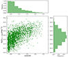 |
Fig. 1. Distribution in the (intrinsic) LX–redshift plane of the 2677 X-ray AGNs used in our analysis. |
3.3. Classification of AGNs
To classify AGNs into type 1 and 2 sources, we used the SED fitting measurements. Specifically, we employed the Bayes and best estimates of the inclination, i, parameter, derived by CIGALE. We followed the criteria applied by Mountrichas et al. (2021a) and Mountrichas & Georgantopoulos (2024) and classified as type 1 those with ibest = 30° and ibayes < 40°, while type 2 sources are those with ibest = 70° and ibayes > 60°.
In Mountrichas et al. (2021a), CIGALE’s classification was compared with the categorization provided in the catalog presented by Menzel et al. (2016). In this catalog, AGNs were divided into two categories: broad-line (type 1) and narrow-line (type 2) sources, based on the full width half maximum (FWHM) of emission lines originating from different regions of the AGN, including Hβ, MgII, CIII, and CIV. The analysis reveals that CIGALE exhibits an accuracy of approximately 85% in classifying type 1 AGNs. A similar level of accuracy is observed for the completeness of type 1 source identification. However, for type 2 sources, CIGALE’s performance is approximately 50%, both in terms of reliability and completeness. The reliability is defined as the fraction of the number of type 1 (or type 2) sources classified by the SED fitting that are similarly classified by optical spectra. The completeness refers to how many sources classified as type 1 (or type 2) based on optical spectroscopy were identified as such by the SED fitting results. For the purposes of our current study, our primary focus is evaluating the reliability performance of CIGALE.
The reliability of approximately 85% in CIGALE’s identification of type 1 sources meets our acceptability criteria for the purposes of our statistical analysis. However, the reliability of the SED fitting code in the case of type 2 AGNs is lower, suggesting that roughly half of the sources classified as type 2 by CIGALE are indeed misclassified. Nonetheless, Mountrichas et al. (2021a) demonstrates that the majority (∼82%) of these misclassified type 2 sources exhibit elevated polar dust values (EB − V > 0.15; see their Fig. 8 and Sect. 5.1.1). Consequently, we excluded these sources from our analysis and categorized as type 2 those AGNs that meet the specified inclination angle criteria and also possess polar dust values lower than EB − V < 0.15 (i.e., similar to the type 2 classification criteria applied in Mountrichas & Georgantopoulos 2024). It is worth noting that the inclusion of polar dust in the fitting process enhances the accuracy of CIGALE’s source type classification, particularly in terms of the reliability of identifying type 2 sources (see Sect. 5.5 in Mountrichas et al. 2021b).
The application of these criteria on the 2677 AGNs (see previous section) results in 825 type 1 and 355 type 2 AGNs. Their LX–redshift distribution is presented in Fig. 2. These are the sources used in the second part of our analysis (Sect. 4.2).
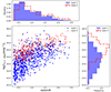 |
Fig. 2. Distribution in the LX–redshift plane of the 825 type 1 (blue triangles) and 355 type 2 (red circles) AGNs used in our analysis. |
4. Results
In this section, we present the results of our analysis. Specifically, we investigate the SFRnorm − LX relation, for galaxies of different M* and for different AGN types.
4.1. SFRnorm as a function of LX and M*
To perform a comparison between the SFR of AGN and non-AGN galaxies, we followed the methodology presented, for instance, in Mountrichas et al. (2021a, 2022a,b, 2023), Mountrichas & Buat (2023). Specifically, we employed the SFRnorm parameter. For the calculation of SFRnorm, we utilized the galaxy control sample presented in Sect. 3. Utilizing a galaxy reference catalog minimizes systematic effects that may affect the accuracy of the SFRnorm calculation, compared to using analytical expressions from the literature (e.g., Schreiber et al. 2015) for the calculation of the SFR of non-AGN galaxies (Mountrichas et al. 2021a).
To measure the SFRnorm parameter, we divided the SFR of each X-ray AGN by the SFR of galaxies in the control sample that closely match the AGN in terms of M* within ±0.2 dex and redshift within ±0.075 × (1 + z). Furthermore, each source’s contribution was weighted based on the uncertainties associated with the SFR and M* measurements obtained using the CIGALE methodology. The median values of these ratios were subsequently utilized as the SFRnorm for each X-ray AGN. It’s worth noting that our measurements were not significantly affected by the specific size of the region surrounding the AGN. However, selecting smaller regions does have an impact on the accuracy of the calculations, as is discussed in Mountrichas et al. (2021a).
The results of our measurements are presented in Fig. 3. Each panel corresponds to systems with a different M* range. Previous studies have shown that there is no (strong) evolution of the SFRnorm − LX relation with redshift (Mountrichas et al. 2021a, 2022a,b). Therefore, we do not split our measurements into different redshift intervals. Median values of SFRnorm and LX are presented. The bins are grouped in bins of LX, of 0.5 dex width, with the exception of the lowest M* range, where an LX bin size of 1 dex was chosen, due to the low number of X-ray sources with 9.5 < log [M*(M⊙)] < 10.0. The errors presented are 1σ, calculated using bootstrap resampling. Only bins that include ten or more sources are presented in the plots. We have overlaid our results with those presented in Fig. 5 in Mountrichas et al. (2022a), where they amalgamate findings from a similar analysis based on data in the Boötes, COSMOS, and eFEDS fields. Furthermore, we have incorporated data from a study conducted by Mountrichas et al. (2024) that employed X-ray AGN data from the XMM-XXL field. It is important to highlight that while the latter study investigated the SFRnorm − LX relationship for systems falling within the range of 10.5 < log [M*(M⊙)] < 11.5, we have opted to compare their results with our findings within the range of 11.0 < log [M*(M⊙)] < 11.5. Additionally, it is worth noting that their results do not include the exclusion of quiescent systems from the X-ray and galaxy control samples.
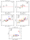 |
Fig. 3. SFRnorm vs. X-ray luminosity for five stellar-mass bins. We complement our results (filled black circles) with those using the Boöes (Mountrichas et al. 2021a), COSMOS (Mountrichas et al. 2022b), eFEDS (Mountrichas et al. 2022a), and XMM-XXL (Mountrichas et al. 2024) datasets. The dashed horizontal line indicates the SFRnorm value (=1) for which the SFR of the AGN is equal to the SFR of non-AGN star-forming galaxies. The measurements are grouped in bins of LX, of 0.5 dex width, with the exception of the lowest M* range, where an LX bin size of 1 dex was chosen. Median values of SFRnorm and LX are presented. Errors were calculated using bootstrap resampling. |
For systems with intermediate M*, that is, 10.5 < log [M*(M⊙)] < 11.0 and 11.0 < log [M*(M⊙)] < 11.5, presented in the left and right panels of the middle row of Fig. 3, we confirm the results of prior studies. Specifically, we find that AGNs with low-to-intermediate LX (log [LX,2−10 keV(erg s−1)] < 44) present lower or at most equal SFRs as those of non-AGN galaxies (SFRnorm ≤ 1), while more luminous AGNs have enhanced SFRs by 20–30% compared to galaxies without an AGN.
More importantly, we observe that for the most massive systems (bottom panel in Fig. 3), the SFRnorm − LX relation remains relatively constant up to an LX threshold, mirroring the observed trend in systems with 10.5 < log [M*(M⊙)] < 11.5. However, the position of this threshold is higher in the case of these massive systems, at log,[LX,2−10 keV(erg s−1)] = 45. Beyond this threshold, we detect a substantial increase, roughly by a factor of two, in the SFR of galaxies hosting an AGN in comparison to those without an AGN. Compared to previous studies, our findings may seem slightly lower; however, they are statistically consistent with those earlier results. Notably, our findings reaffirm previous observations of a substantial elevation in SFRnorm at a very high LX. Specifically, in a study by Mountrichas et al. (2022a), data derived from the eFEDS field, incorporating X-ray observations from the eROSITA satellite, reveal a significant rise in SFRnorm at an LX of approximately log [LX,2−10 keV(erg s−1)] ≈ 45. However, their dataset did not span higher LX values to ascertain whether this result was consistent or merely a statistical fluctuation. Our measurements validate the notion that, in the most massive systems, galaxies with an AGN exhibit heightened SFRs in comparison to non-AGN galaxies; however, this enhancement is only observed at very high LX.
The outcomes pertaining to the least massive systems within our datasets are depicted in the upper panels of Fig. 3. In the case of galaxies falling within the range of 10.0 < log [M*(M⊙)] < 10.5, we observe an augmentation in the SFR of AGN-hosting galaxies in comparison to non-AGN ones (indicated by SFRnorm > 1). This phenomenon mirrors what is seen in systems with an intermediate stellar mass (i.e., 10.5 < log [M*(M⊙)] < 11.5). However, it is worth noting that this increase in the SFRnorm parameter is detected at lower values of LX (i.e., approximately log [LX,2−10 keV(erg s−1)] ∼ 43 − 43.5), as opposed to the intermediate stellar mass galaxies where it occurs at around log [LX,2−10 keV(erg s−1)] ∼ 44.
Our results are in agreement with prior studies that have reported either a lower or similar SFR between low-to-moderate LX AGN and non-AGN galaxies (e.g., Shimizu et al. 2015, 2017; Masoura et al. 2018; Bernhard et al. 2019) and an enhanced SFR of luminous AGNs compared to their non-AGN counterparts (e.g., Florez et al. 2020; Pouliasis et al. 2022). Our findings also underline the importance of M* in the comparison of the SFRs of the two populations, similar to the results from recent studies (e.g., Torbaniuk et al. 2021, 2023).
Overall, our findings underscore that the assessment of SFRs in AGN-hosting and non-AGN galaxies hinges on both the power of AGN (LX) and the M* of the hosting galaxy. Our results suggest that galaxies with an AGN tend to exhibit an elevated SFR when contrasted with those lacking an AGN, after an LX threshold. However, the point at which the AGNs start to present an enhanced SFR compared to non-AGNs (i.e., SFRnorm > 1) varies depending on the M* of the host galaxy. More precisely, the threshold LX value for this enhancement increases as we transition to more massive galactic systems. These findings align with a hypothesis wherein AGN feedback, potentially manifested as strong winds (e.g., DeBuhr et al. 2012), could lead to the over-compression of existing cold gas within the host galaxy (e.g., Zubovas et al. 2013), consequently promoting star formation (positive feedback). The more massive the host galaxy, the stronger (more luminous) the AGN needs to be in order to exert an impact on the star formation within its host.
Lastly, Fig. 4 consolidates all our findings across different ranges of M*. We observe that, for the same LX, the amplitude of the SFRnorm parameter diminishes as we transition to more massive galaxies, at least up to log [LX,2−10 keV(erg s−1)] = 45. This could be attributed to the fact that in galaxies that host an AGN the increase in the SFR with rising M* is not as pronounced as it is in galaxies devoid of AGNs. This variation could be a result of some of the available gas being channeled toward fueling the SMBH instead. This scenario implies that the X-ray main sequence (Aird et al. 2018) has a less steep slope compared to the galaxy main sequence. Figure 5 presents the SFR versus M* for X-ray AGN and non-AGN galaxies, at different redshift intervals, as is indicated in the legend of the plot. Within the redshift range of 0.3 < z < 1.0, we observe a slope of 0.21 ± 0.04 for AGN-hosting galaxies and 0.48 ± 0.01 for non-AGN ones. In the redshift range of 1.0 < z < 2.0, AGN galaxies exhibit a slope of 0.50 ± 0.04, while galaxies without an AGN display a slope of 0.88 ± 0.02. Utilizing mean square error (MSE) analysis demonstrates an excellent goodness of fit for all the models (MSE value < 0.5 in all instances). Additionally, consistent fits are achieved when employing the linmix module (Kelly 2007), which conducts linear regression between two parameters by iteratively perturbing the data points within their uncertainties. These findings reinforce the interpretation mentioned earlier.
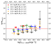 |
Fig. 4. Compilation of our SFRnorm − LX measurements for different stellar masses, as is indicated in the legend of the figure. |
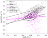 |
Fig. 5. SFR vs. M*, for the X-ray AGN and non-AGN galaxies in our dataset, at different redshift intervals, as is indicated in the legend. Lines show the best fits for each subset. |
4.2. SFRnorm − LX for type 1 and 2 AGNs
In this section, we compare the SFRnorm − LX relation for different AGN types. For that purpose, we classified the X-ray sources into type 1 and 2 AGNs, using the results of CIGALE, as is described in Sect. 3.3. Additionally, we narrowed down our selection to sources falling within the M* range of 10.5 < log [M*(M⊙)] < 11.5. We made this choice because, as both our study and previous research have indicated, the SFRnorm − LX relationship exhibits similarities within this M* range. This filtering reduced the number of AGNs available for our analysis to 652 type 1 AGNs and 293 type 2 AGNs.
The results are presented in Fig. 6. Measurements are grouped in LX bins of size 1 dex. As was previously mentioned, we only present bins that include ≥10 sources. We notice that type 1 AGNs have higher SFRnorm values compared to type 2 ones, at least for AGNs with an LX within the range of 43.5 < log [LX,2−10 keV(erg s−1)] < 45. Furthermore, within this LX range, we observe that type 1 AGNs appear to have higher SFRs compared to non-AGN galaxies of similar M* and redshift (i.e., SFRnorm > 1). On the contrary, type 2 AGNs tend to have lower SFRs compared to galaxies without an AGN.
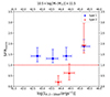 |
Fig. 6. SFRnorm − LX for different AGN types, at 0.3 < z < 2.5. |
Masoura et al. (2021) conducted a study involving more than 3000 X-ray AGNs in the XMM-XXL field, focusing on the SFRnorm − LX relationship for X-ray obscured and unobscured sources. Their classification criterion was based on the hydrogen column density, NH. Specifically, they categorized sources with NH > 1021.5 cm−2 as absorbed sources. According to their findings, they did not identify significant distinctions in the SFRnorm as a function of LX between the two AGN categories. We note, though, that as several previous studies have emphasized, the adoption of different criteria for characterizing AGNs based on their level of obscuration can lead to varying categorizations of AGNs (e.g., Merloni et al. 2014; Li et al. 2019; Masoura et al. 2020; Mountrichas et al. 2021a).
Some prior studies that compared the SFRs of type 1 and 2 AGNs, using optical spectra for the classification, did not discover significant differences in the SFRs of the two AGN populations (Zou et al. 2019; Mountrichas et al. 2021a). However, it is crucial to emphasize that the AGNs in these studies covered, mainly, lower LX values (log[LX,2−10 keV(erg s−1)] < 44) compared to our sources. Earlier research has underlined that the comparison of the host galaxy properties of different AGN types depends on the LX regime under consideration (Georgantopoulos et al. 2023). Mountrichas & Georgantopoulos (2024) employed X-ray sources in the eFEDS and COSMOS fields and classified them into type 1 and 2, using CIGALE’s classification measurements, akin to our approach. According to their findings, the comparison of the SFR of type 1 and 2 AGN depends on both redshift and LX. Specifically, they find that type 1 AGNs tend to have a higher SFR compared to type 2 sources, for sources with log[LX,2−10 keV(erg s−1)] < 44, at all redshifts spanned by their dataset (0.5 < z < 3.5). Based on their results, this picture reverses at z > 2 and log [LX,2−10 keV(erg s−1)] > 44. At intermediate redshift ranges (1 < z < 2) and for log[LX,2−10 keV(erg s−1)] > 44 the two AGN populations appear to have a similar SFR.
In light of these findings, we divided our AGN sample into two redshift intervals, that is, 0.3 ≤ z ≤ 1.0 and 1.0 ≤ z ≤ 2.0. At z > 2, we lack a sufficient number of type 2 sources to perform a meaningful analysis. The results are presented in Fig. 7. Notably, in the lower redshift interval (top panel), type 1 AGNs appear to have higher SFRnorm values compared to type 2 ones, while at the higher redshift range (bottom panel) the two AGN types exhibit consistent SFRnorm measurements. Although the number of available sources for this exercise, and in particular the number of type 2 AGNs, is not sufficiently large for strong conclusions to be drawn, these results appear to be in line with those presented in Mountrichas & Georgantopoulos (2024). Moreover, for type 2 AGNs, SFRnorm increases with LX at both redshift intervals, while for type 1 ones it remains roughly constant at low redshifts and increases with LX at z > 1.
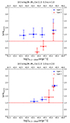 |
Fig. 7. SFRnorm − LX for type 1 (red triangles) and type 2 (blue squares) AGNs. The top panel presents the results at 0.3 ≤ z < 1.0. The bottom panel shows the measurements for sources within 1.0 ≤ z < 2.0. |
The observed SFRnorm > 1 for type 1 AGNs in the specified LX range suggests a potential positive feedback mechanism, where the presence of a type 1 AGN enhances star formation beyond what is typical for galaxies without an AGN. Type 1 AGNs typically exhibit a clearer view of the central engine due to the absence of significant obscuration. This unimpeded view may lead to a more direct interaction between the AGN and the surrounding gas, potentially influencing star formation. The distinct behavior of type 1 AGNs, where SFRnorm remains relatively constant at low redshifts and increases with LX at higher redshifts, might indicate that the feedback mechanisms associated with type 1 AGNs evolve differently over cosmic time. The lower SFRnorm in type 2 AGNs, at least at z < 1, may imply that the gas reservoirs in type 2 AGN host galaxies are less conducive to star formation, potentially due to feedback effects from the AGN. However, larger samples are required for strong conclusions to be drawn.
5. Conclusions
In this work, we compiled a dataset comprising 2677 X-ray AGNs detected by the XMM satellite, along with a control sample of 64 557 galaxies without an AGN, all of which lie in the 3XMM footprint. We constructed SEDs for these sources by using photometric data from the DES, VHS, and AllWISE surveys and employed the CIGALE SED fitting code to obtain measurements for their (host) galaxy properties. Our sources span a wide parameter space, with objects falling within the ranges of 9.5 < log [M*(M⊙)] < 12.0, 42 < log [LX,2−10 keV(erg s−1)] < 45.5, and 0.3 < z < 2.5. Leveraging CIGALE’s measurements, we classified AGNs into types 1 and 2. In our analysis, we used 652 type 1 AGNs and 293 type 2 ones within a M* range of 10.5 < log [M*(M⊙)] < 11.5. The main results of our investigation can be summarized as follows:
-
The comparison of the SFR of AGN and non-AGN galaxies hinges on both the LX and the stellar mass. Specifically, AGN systems tend to present an enhanced SFR when compared to non-AGN systems, but the LX at which this elevation becomes apparent increases as we transition to more massive galactic systems.
-
For the same LX, the amplitude of the SFRnorm parameter decreases as we move to more massive galaxies. This could be attributed to the fact that in galaxies with an AGN the increase in SFR with rising M* is not as evident as it is in galaxies without an AGN. This scenario is supported by the less steep slope that we observe for the X-ray star-forming main sequence compared to the galaxy main sequence.
-
For systems with 10.5 < log [M*(M⊙)] < 11.5, type 1 AGNs tend to exhibit a higher SFR compared to type 2 ones, at matching LX and M*, at z < 1. However, at higher redshifts the two AGN populations present a similar SFR.
-
At low redshifts (z < 1) and 10.5 < log [M*(M⊙)] < 11.5, type 1 AGNs have an enhanced SFR compared to non-AGN systems, with similar M* and redshift. On the contrary, type 2 AGNs have a lower SFR compared to galaxies without an AGN, at least up to log [LX,2−10 keV(erg s−1)] < 45.
-
At higher redshifts (z > 1) and 10.5 < log [M*(M⊙)] < 11.5, both type 1 and type 2 AGNs tend to have a higher SFR than non-AGN galaxies with similar redshift and M*.
Acknowledgments
This project has received funding from the European Union’s Horizon 2020 research and innovation program under grant agreement no. 101004168, the XMM2ATHENA project. VAM acknowledges support by the Grant RTI2018-096686-B-C21 funded by MCIN/AEI/10.13039/501100011033 and by ’ERDF A way of making Europe’. AC and FJC acknowledge support by the Grant PID2021-122955OB-C41 funded by MCIN/AEI/10.13039/501100011033 and by ERDF A way of making Europe. This research has made use of TOPCAT version 4.8 (Taylor 2005) and Astropy (Astropy Collaboration 2022).
References
- Abbott, T. M. C., Abdalla, F. B., Allam, S., et al. 2018, ApJS, 239, 18 [Google Scholar]
- Aird, J., Coil, A. L., & Georgakakis, A. 2018, MNRAS, 474, 1225 [NASA ADS] [CrossRef] [Google Scholar]
- Akylas, A., Georgantopoulos, I., Georgakakis, A., Kitsionas, S., & Hatziminaoglou, E. 2006, A&A, 459, 693 [NASA ADS] [CrossRef] [EDP Sciences] [Google Scholar]
- Astropy Collaboration (Price-Whelan, A. M., et al.) 2022, ApJ, 935, 167 [NASA ADS] [CrossRef] [Google Scholar]
- Bernhard, E., Grimmett, L. P., Mullaney, J. R., et al. 2019, MNRAS, 483, L52 [NASA ADS] [CrossRef] [Google Scholar]
- Boquien, M., Burgarella, D., Roehlly, Y., et al. 2019, A&A, 622, A103 [NASA ADS] [CrossRef] [EDP Sciences] [Google Scholar]
- Brandt, W. N., & Alexander, D. M. 2015, A&ARv, 23, 1 [Google Scholar]
- Bruzual, G., & Charlot, S. 2003, MNRAS, 344, 1000 [NASA ADS] [CrossRef] [Google Scholar]
- Buat, V., Ciesla, L., Boquien, M., Małek, K., & Burgarella, D. 2019, A&A, 632, A79 [NASA ADS] [CrossRef] [EDP Sciences] [Google Scholar]
- Buat, V., Mountrichas, G., Yang, G., et al. 2021, A&A, 654, A93 [NASA ADS] [CrossRef] [EDP Sciences] [Google Scholar]
- Charlot, S., & Fall, S. M. 2000, ApJ, 539, 718 [Google Scholar]
- Ciotti, L., & Ostriker, J. P. 1997, ApJ, 487, L105 [NASA ADS] [CrossRef] [Google Scholar]
- Dale, D. A., Helou, G., Magdis, G. E., et al. 2014, ApJ, 784, 83 [Google Scholar]
- DeBuhr, J., Quataert, E., & Ma, C.-P. 2012, MNRAS, 420, 2221 [NASA ADS] [CrossRef] [Google Scholar]
- Elbaz, D., Daddi, E., Borgne, D. L., et al. 2007, A&A, 468, 33 [NASA ADS] [CrossRef] [EDP Sciences] [Google Scholar]
- Florez, J., Jogee, S., Sherman, S., et al. 2020, MNRAS, 497, 3273 [NASA ADS] [CrossRef] [Google Scholar]
- Georgantopoulos, I., Pouliasis, E., Mountrichas, G., et al. 2023, A&A, 673, A67 [NASA ADS] [CrossRef] [EDP Sciences] [Google Scholar]
- Harrison, C. M., Alexander, D. M., Swinbank, A. M., et al. 2012, ApJ, 760, 5 [Google Scholar]
- Hopkins, P. F., Hernquist, L., Cox, T. J., et al. 2006, ApJS, 163, 1 [Google Scholar]
- Kelly, B. C. 2007, ApJ, 665, 1489 [Google Scholar]
- Koutoulidis, L., Mountrichas, G., Georgantopoulos, I., Pouliasis, E., & Plionis, M. 2022, A&A, 658, A35 [NASA ADS] [CrossRef] [EDP Sciences] [Google Scholar]
- Laigle, C., McCracken, H. J., Ilbert, O., et al. 2016, ApJS, 224, 24 [Google Scholar]
- Li, J., Xue, Y., Sun, M., et al. 2019, ApJ, 877, 5 [NASA ADS] [CrossRef] [Google Scholar]
- Lutz, D., Mainieri, V., Rafferty, D., et al. 2010, ApJ, 712, 1287 [NASA ADS] [CrossRef] [Google Scholar]
- Małek, K., Buat, V., Roehlly, Y., et al. 2018, A&A, 620, A50 [Google Scholar]
- Masoura, V. A., Mountrichas, G., Georgantopoulos, I., et al. 2018, A&A, 618, A31 [NASA ADS] [CrossRef] [EDP Sciences] [Google Scholar]
- Masoura, V. A., Georgantopoulos, I., Mountrichas, G., et al. 2020, A&A, 638, A45 [NASA ADS] [CrossRef] [EDP Sciences] [Google Scholar]
- Masoura, V. A., Mountrichas, G., Georgantopoulos, I., & Plionis, M. 2021, A&A, 646, A167 [EDP Sciences] [Google Scholar]
- McMahon, R. G., Banerji, M., Gonzalez, E., et al. 2013, The Messenger, 154, 35 [NASA ADS] [Google Scholar]
- Menzel, M.-L., Merloni, A., Georgakakis, A., et al. 2016, MNRAS, 457, 110 [Google Scholar]
- Merloni, A., Bongiorno, A., Brusa, M., et al. 2014, MNRAS, 437, 3550 [Google Scholar]
- Morganti, R. 2017, Nat. Astron., 1, 39 [NASA ADS] [CrossRef] [Google Scholar]
- Mountrichas, G. 2023, A&A, 672, A98 [NASA ADS] [CrossRef] [EDP Sciences] [Google Scholar]
- Mountrichas, G., & Buat, V. 2023, A&A, 679, A151 [NASA ADS] [CrossRef] [EDP Sciences] [Google Scholar]
- Mountrichas, G., & Shankar, F. 2023, MNRAS, 518, 2088 [Google Scholar]
- Mountrichas, G., & Georgantopoulos, I. 2024, A&A, in press, https://doi.org/10.1051/0004-6361/202348156 [NASA ADS] [CrossRef] [EDP Sciences] [Google Scholar]
- Mountrichas, G., Buat, V., Georgantopoulos, I., et al. 2021a, A&A, 653, A70 [NASA ADS] [CrossRef] [EDP Sciences] [Google Scholar]
- Mountrichas, G., Buat, V., Yang, G., et al. 2021b, A&A, 646, A29 [EDP Sciences] [Google Scholar]
- Mountrichas, G., Buat, V., Yang, G., et al. 2021c, A&A, 653, A74 [NASA ADS] [CrossRef] [EDP Sciences] [Google Scholar]
- Mountrichas, G., Buat, V., Yang, G., et al. 2022a, A&A, 663, A130 [NASA ADS] [CrossRef] [EDP Sciences] [Google Scholar]
- Mountrichas, G., Masoura, V. A., Xilouris, E. M., et al. 2022b, A&A, 661, A108 [NASA ADS] [CrossRef] [EDP Sciences] [Google Scholar]
- Mountrichas, G., Yang, G., Buat, V., et al. 2023, A&A, 675, A137 [NASA ADS] [CrossRef] [EDP Sciences] [Google Scholar]
- Mountrichas, G., Siudek, M., & Cucciati, O. 2024, A&A, submitted [NASA ADS] [CrossRef] [EDP Sciences] [Google Scholar]
- Mullaney, J. R., Alexander, D. M., Aird, J., et al. 2015, MNRAS, 453, L83 [Google Scholar]
- Nenkova, M., Ivezić, Ž., & Elitzur, M. 2002, ApJ, 570, L9 [NASA ADS] [CrossRef] [Google Scholar]
- Netzer, H. 2015, ARA&A, 53, 365 [Google Scholar]
- Noeske, K. G., Weiner, B. J., Faber, S. M., et al. 2007, ApJ, 660, L43 [CrossRef] [Google Scholar]
- Page, M. J., Symeonidis, M., Vieira, J. D., et al. 2012, Nature, 485, 213 [NASA ADS] [CrossRef] [Google Scholar]
- Pineau, F. X., Derriere, S., Motch, C., et al. 2017, A&A, 597, A28 [NASA ADS] [CrossRef] [EDP Sciences] [Google Scholar]
- Pouliasis, E., Mountrichas, G., Georgantopoulos, I., et al. 2020, MNRAS, 495, 1853 [NASA ADS] [CrossRef] [Google Scholar]
- Pouliasis, E., Mountrichas, G., Georgantopoulos, I., et al. 2022, A&A, 667, A56 [NASA ADS] [CrossRef] [EDP Sciences] [Google Scholar]
- Pozzetti, L., Bolzonella, M., Zucca, E., et al. 2010, A&A, 523, A23 [Google Scholar]
- Rosario, D. J., Santini, P., Lutz, D., et al. 2012, A&A, 545, A18 [Google Scholar]
- Rosario, D. J., Trakhtenbrot, B., Lutz, D., et al. 2013, A&A, 560, A72 [NASA ADS] [CrossRef] [EDP Sciences] [Google Scholar]
- Rosen, S. R., Webb, N. A., Watson, M. G., et al. 2016, A&A, 590, A1 [NASA ADS] [CrossRef] [EDP Sciences] [Google Scholar]
- Rovilos, E., Comastri, A., Gilli, R., et al. 2012, A&A, 546, A16 [NASA ADS] [CrossRef] [EDP Sciences] [Google Scholar]
- Ruiz, A., Corral, A., Mountrichas, G., & Georgantopoulos, I. 2018, A&A, 618, A52 [NASA ADS] [CrossRef] [EDP Sciences] [Google Scholar]
- Santini, P., Rosario, D. J., Shao, L., et al. 2012, A&A, 540, A109 [NASA ADS] [CrossRef] [EDP Sciences] [Google Scholar]
- Schreiber, C., Pannella, M., Elbaz, D., et al. 2015, A&A, 575, A29 [NASA ADS] [CrossRef] [EDP Sciences] [Google Scholar]
- Shimizu, T. T., Mushotzky, R. F., Meléndez, M., Koss, M., & Rosario, D. J. 2015, MNRAS, 452, 1841 [NASA ADS] [CrossRef] [Google Scholar]
- Shimizu, T. T., Mushotzky, R. F., Meléndez, M., et al. 2017, MNRAS, 466, 3161 [NASA ADS] [CrossRef] [Google Scholar]
- Speagle, J. S., Steinhardt, C. L., Capak, P. L., & Silverman, J. D. 2014, ApJS, 214, 15 [Google Scholar]
- Stalevski, M., Fritz, J., Baes, M., Nakos, T., & Popović, L. Č. 2012, MNRAS, 420, 2756 [Google Scholar]
- Stalevski, M., Ricci, C., Ueda, Y., et al. 2016, MNRAS, 458, 2288 [Google Scholar]
- Taylor, M. B. 2005, in Astronomical Data Analysis Software and Systems XIV, eds. P. Shopbell, M. Britton, & R. Ebert, ASP Conf. Ser., 347, 29 [Google Scholar]
- Torbaniuk, O., Paolillo, M., Carrera, F., et al. 2021, MNRAS, 506, 2619 [NASA ADS] [CrossRef] [Google Scholar]
- Torbaniuk, O., Paolillo, M., D’Abrusco, R., et al. 2023, MNRAS, 527, 12091 [NASA ADS] [CrossRef] [Google Scholar]
- Urry, C. M., & Padovani, P. 1995, PASP, 107, 803 [NASA ADS] [CrossRef] [Google Scholar]
- Villa-Velez, J. A., Buat, V., Theule, P., Boquien, M., & Burgarella, D. 2021, A&A, 654, A153 [NASA ADS] [CrossRef] [EDP Sciences] [Google Scholar]
- Whitaker, K. E., van Dokkum, P. G., Brammer, G., & Franx, M. 2012, ApJ, 754, L29 [Google Scholar]
- Wright, E. L., Eisenhardt, P. R. M., Mainzer, A. K., et al. 2010, AJ, 140, 1868 [Google Scholar]
- Yang, G., Boquien, M., Buat, V., et al. 2020, MNRAS, 491, 740 [Google Scholar]
- Yang, G., Boquien, M., Brandt, W. N., et al. 2022, ApJ, 927, 192 [NASA ADS] [CrossRef] [Google Scholar]
- Zou, F., Yang, G., Brandt, W. N., & Xue, Y. 2019, ApJ, 878, 11 [Google Scholar]
- Zubovas, K., Nayakshin, S., King, A., & Wilkinson, M. 2013, MNRAS, 433, 3079 [Google Scholar]
All Figures
|
Fig. 1. Distribution in the (intrinsic) LX–redshift plane of the 2677 X-ray AGNs used in our analysis. |
| In the text | |
|
Fig. 2. Distribution in the LX–redshift plane of the 825 type 1 (blue triangles) and 355 type 2 (red circles) AGNs used in our analysis. |
| In the text | |
|
Fig. 3. SFRnorm vs. X-ray luminosity for five stellar-mass bins. We complement our results (filled black circles) with those using the Boöes (Mountrichas et al. 2021a), COSMOS (Mountrichas et al. 2022b), eFEDS (Mountrichas et al. 2022a), and XMM-XXL (Mountrichas et al. 2024) datasets. The dashed horizontal line indicates the SFRnorm value (=1) for which the SFR of the AGN is equal to the SFR of non-AGN star-forming galaxies. The measurements are grouped in bins of LX, of 0.5 dex width, with the exception of the lowest M* range, where an LX bin size of 1 dex was chosen. Median values of SFRnorm and LX are presented. Errors were calculated using bootstrap resampling. |
| In the text | |
|
Fig. 4. Compilation of our SFRnorm − LX measurements for different stellar masses, as is indicated in the legend of the figure. |
| In the text | |
|
Fig. 5. SFR vs. M*, for the X-ray AGN and non-AGN galaxies in our dataset, at different redshift intervals, as is indicated in the legend. Lines show the best fits for each subset. |
| In the text | |
|
Fig. 6. SFRnorm − LX for different AGN types, at 0.3 < z < 2.5. |
| In the text | |
|
Fig. 7. SFRnorm − LX for type 1 (red triangles) and type 2 (blue squares) AGNs. The top panel presents the results at 0.3 ≤ z < 1.0. The bottom panel shows the measurements for sources within 1.0 ≤ z < 2.0. |
| In the text | |
Current usage metrics show cumulative count of Article Views (full-text article views including HTML views, PDF and ePub downloads, according to the available data) and Abstracts Views on Vision4Press platform.
Data correspond to usage on the plateform after 2015. The current usage metrics is available 48-96 hours after online publication and is updated daily on week days.
Initial download of the metrics may take a while.