| Issue |
A&A
Volume 679, November 2023
|
|
|---|---|---|
| Article Number | A151 | |
| Number of page(s) | 10 | |
| Section | Extragalactic astronomy | |
| DOI | https://doi.org/10.1051/0004-6361/202347392 | |
| Published online | 30 November 2023 | |
Link between star formation and the properties of supermassive black holes
1
Instituto de Fisica de Cantabria (CSIC-Universidad de Cantabria), Avenida de los Castros, 39005 Santander, Spain
e-mail: This email address is being protected from spambots. You need JavaScript enabled to view it.
2
Aix-Marseille Univ., CNRS, CNES, LAM, Marseille, France
3
Institut Universitaire de France (IUF), Marseille, France
Received:
7
July
2023
Accepted:
27
September
2023
Abstract
It is well known that supermassive black holes (SMBHs) and their host galaxies undergo a process of co-evolution. Feedback from active galactic nuclei (AGNs) plays an important role in this symbiosis. To study the effect of AGN feedback on the host galaxy, one popular method is to study the star formation rate (SFR) as a function of the X-ray luminosity (LX). However, hydrodynamical simulations suggest that the cumulative impact of AGN feedback on a galaxy is encapsulated in the mass of the SMBH, MBH, rather than the LX. In this study, we compare the SFRs of AGN and non-AGN galaxies as a function of LX, MBH, the Eddington ratio (nEdd), and the specific black hole accretion rate (λsBHAR). For that purpose, we used 122 X-ray AGN in the XMM-XXL field and 3371 galaxies from the VIPERS survey to calculate the SFRnorm parameter, defined as the ratio of the SFR of AGN to the SFR of non-AGN galaxies with similar stellar mass, M*, and redshift. Our datasets span a redshift range of 0.5 ≤ z ≤ 1.2. The results show that the correlation between SFRnorm and MBH is stronger compared to that between SFRnorm and LX. A weaker correlation is found between SFRnorm and λsBHAR. No correlation is detected between SFRnorm and nEdd. These results corroborate the notion that the MBH is a more robust tracer of the cumulative impact of the AGN feedback, compared to the instantaneous accretion rate (LX). Thus, it may serve as a better predictive parameter of changes in the SFR of the host galaxy.
Key words: galaxies: active / galaxies: evolution / galaxies: star formation / X-rays: galaxies / X-rays: general
© The Authors 2023
 Open Access article, published by EDP Sciences, under the terms of the Creative Commons Attribution License (https://creativecommons.org/licenses/by/4.0), which permits unrestricted use, distribution, and reproduction in any medium, provided the original work is properly cited.
This article is published in open access under the Subscribe to Open model. This email address is being protected from spambots. You need JavaScript enabled to view it. to support open access publication.
1. Introduction
The supermassive black holes (SMBHs) that live in the centre of galaxies become active when material that is in the vicinity of the SMBH is accreted onto them. A great deal of evidence presented over the past two decades has shown that a co-evolution between the SMBH and its host galaxy exists. For instance, both the activity of the black hole and the star formation (SF) of galaxies are fed by the same material (i.e., cold gas) and both phenomena peak at about the same cosmic time (z ∼ 2; e.g., Boyle et al. 2000; Sobral et al. 2013). Moreover, tight correlations have been found in the Local Universe, between the mass of the SMBH, MBH, and various properties of the host galaxy, such as the stellar velocity dispersion the bulge luminosity and the bulge mass (e.g., Magorrian et al. 1998; Ferrarese & Merritt 2000; Tremaine et al. 2002; Häring & Rix 2004). These correlations also seem to exist at higher redshifts (z ∼ 2; e.g., Jahnke et al. 2009; Merloni et al. 2010; Sun et al. 2015; Suh et al. 2020; Setoguchi et al. 2021; Mountrichas 2023).
Various mechanisms have been suggested that drive the gas from kiloparsec to sub-parsec scales (for a review see Alexander & Hickox 2012). Also, AGN feedback in the form of jets, radiation, or winds has been included in most simulations to explain many galaxy properties, with respect to the way the hot intracluster medium is maintained (e.g., Dunn & Fabian 2006), the shape of the galaxy stellar mass function is formed (e.g., Bower et al. 2012), and the galaxy morphology is composed (e.g., Dubois et al. 2016).
A popular method to study the symbiosis between the AGN and its host galaxy is to examine the correlation between the star formation rate (SFR) and the power of AGN, using the X-ray luminosity (LX) as a proxy for the latter. Most prior studies have found a positive correlation between the SFR and LX (e.g., Lanzuisi et al. 2017; Masoura et al. 2018; Brown et al. 2019), whereas no specific correlation was reported in Stanley et al. (2015). However, more information can be gained when we compare the SFR of AGN with the SFR of non-AGN galaxies with similar redshifts and stellar masses, M*, as a function of LX (e.g., Santini et al. 2012; Shimizu et al. 2015, 2017; Florez et al. 2020). In this case, most studies measure what is often call normalized SFR, namely, SFRnorm, which is the ratio of AGN to the ratio of SF main-sequence (MS) galaxies with similar redshift and M* (Rosario et al. 2013; Mullaney et al. 2015; Bernhard et al. 2019). A strong positive correlation has been found between SFRnorm and LX at redshifts of up to z ∼ 5 (Masoura et al. 2021; Koutoulidis et al. 2022; Pouliasis et al. 2022). However, after minimizing systematics effects that may be introduced in the comparison of the SFR of AGN and non-AGN systems (e.g., due to the different methods used to calculate the SFR of the two populations, the different photometric selection criteria that have been applied; for more details, see Mountrichas et al. 2021c), a weaker correlation or even the absence of any correlation is detected between SFRnorm and LX, depending on the M* range (see Fig. 5 in Mountrichas et al. 2022a).
The different trends observed in the SFRnorm − LX relation in different M* regimes, also highlight the importance of M* in this kind of investigations. There are observational works that have found that the black hole accretion rate (BHAR ∝ LX) is mainly linked to M* rather than SFR (Yang et al. 2017). Moreover, SFRnorm appears to be stronger correlated with M* than with LX (Mountrichas et al. 2022a). Theoretical studies that used hydrodynamical simulations have also found that that the cumulative impact of AGN feedback on the host galaxy is encapsulated in the mass of the supermassive black hole, MBH, and not in LX, both in the Local Universe (Piotrowska et al. 2022) and at high redshifts (Bluck et al. 2023). The fact that the SFR shows a strong link both with M* and MBH could be due to the underlying M* − MBH relation that has been found to hold up to at least redshift of 2 (e.g., Merloni et al. 2010; Sun et al. 2015; Setoguchi et al. 2021; Mountrichas 2023).
In this work, we compare the SFR of X-ray detected AGN with that of non-AGN galaxies as a function of different black hole properties. For that purpose, we use X-ray AGN detected in the XMM-XXL field, for which there are available MBH measurements, and a sample of (non-AGN) galaxies from the VIPERS survey that (partially) overlaps with XMM-XXL. We use these two samples to calculate the SFRnorm parameter and examine the correlation of SFRnorm with the LX, MBH, Eddington ratio (nEdd), and specific black hole accretion rate (λsBHAR). Finally, we discuss our results and describe our main conclusions. Throughout this work, we assume a flat ΛCDM cosmology with H0 = 70.4 km s−1 Mpc−1 and ΩM = 0.272 (Komatsu et al. 2011).
2. Data
The main goal of this study is to examine how the SFR of X-ray AGN compares with the SFR of non-AGN systems as a function of various black hole properties. For that purpose, we compiled an X-ray dataset that comprises of AGN detected in the XMM-XXL field and a control sample of (non-AGN) galaxies made up of sources observed by the VIPERS survey. The sky area that the two surveys cover (partially) overlaps. Below, we provide a brief description of these two surveys. The (final) AGN and non-AGN samples used in our analysis are described in Sect. 4.
2.1. The XMM-XXL dataset
The X-ray dataset used in this work consists of X-ray AGN observed in the northern field of the XMM-Newton-XXL survey (XMM-XXL; Pierre et al. 2016). XMM-XXL is a medium-depth X-ray survey that covers a total area of 50 deg2 split into two fields nearly equal in size: the XMM-XXL North (XXL-N) and the XXM-XXL South (XXL-S). The XXL-N dataset consists of 8445 X-ray sources. Of these X-ray sources, 5294 have SDSS counterparts and 2512 have reliable spectroscopy (Menzel et al. 2016; Liu et al. 2016). The mid-IR and near-IR (MIR and NIR) data were obtained following the likelihood ratio method (Sutherland & Saunders 1992) as implemented in (Georgakakis et al. 2011). For more details on the reduction of the XMM observations and the IR identifications of the X-ray sources, we refer to Georgakakis et al. (2017).
2.2. The VIPERS catalogue
The galaxy control sample used in our analysis comes from the public data release 2 (PDR-2; Scodeggio et al. 2018) of the VIPERS survey (Guzzo et al. 2014; Garilli et al. 2014), which partially overlaps with the XMM-XXL field. The observations were carried out using the VIMOS (VIsible MultiObject Spectrograph; Le Fèvre et al. 2003) on the ESO Very Large Telescope (VLT). The survey covers an area of ≈23.5 deg2, split over two regions within the Canada-France-Hawaii Telescope Legacy Survey (CFHTLS-Wide) W1 and W4 fields. Follow-up spectroscopic targets were selected to the magnitude limit i′ = 22.5 from the T0006 data release of the CFHTLS catalogues. An optical colour–colour pre-selection, namely, [(r − i) > 0.5(u − g) or (r − i) > 0.7], excludes galaxies at z < 0.5, yielding a > 98% completeness for z > 0.5 and up to z ∼ 1.2 (for more details see Guzzo et al. 2014). Then, PDR-2 consists of 86 775 galaxies with available spectra. Each spectrum is assigned a quality flag that quantifies the redshift reliability. In all the VIPERS papers, redshifts with flags in the range between 2 and 9 have been considered to be reliable and are those used in the science analysis (Garilli et al. 2014; Scodeggio et al. 2018). The above criteria yield 45 180 galaxies within the redshift range spanned by the VIPERS survey (0.5 < z < 1.2). This is the same galaxy sample used in Mountrichas et al. (2019, see their Sect. 2.1).
To add the NIR and MIR photometry, we cross-matched the VIPERS catalogue with sources in the VISTA Hemisphere Survey (VHS; McMahon et al. 2013) and the AllWISE catalogue from the WISE survey (Wright et al. 2010). The process is described in detail in Sect. 2.5 in Pouliasis et al. (2020). Specifically, the xmatch tool from the astromatch1 package was used. xmatch utilizes different statistical methods for cross-matching of astronomical catalogues. This tool matches a set of catalogues and gives the Bayesian probabilities of the associations or non-association (Pineau et al. 2017). We only kept sources with a high probability of association (> 68%). When one source was associated with several counterparts, we selected the association with the highest probability. 14 128 galaxies from the VIPERS catalogue have counterparts in the NIR and MIR.
3. Galaxy and supermassive black hole properties
In the following, we describe how we obtained measurements for the properties of the sources used in our analysis. Specifically, we present how we measured the SFR and M* of AGN and non-AGN galaxies, how we calculated the bolometric luminosity (Lbol), nEdd and λsBHAR) of AGN, and how the available MBH were estimated.
3.1. Calculation of SFR and M*
For the calculation of the SFR and M* of AGN host galaxies and non-AGN systems, we applied spectral energy distribution (SED) fitting, using the CIGALE algorithm (Boquien et al. 2019; Yang et al. 2020, 2022). CIGALE allows for the inclusion of the X-ray flux in the fitting process and has the ability to account for the extinction of the UV and optical emission in the poles of AGN (Yang et al. 2020; Mountrichas et al. 2021a,b; Buat et al. 2021).
For consistency with our previous studies (Mountrichas et al. 2021c, 2022a,b; Mountrichas & Shankar 2023), we used the same templates and parametric grid in the SED fitting process as those used in these previous works. In brief, the galaxy component is modelled using a delayed SFH model with a function form SFR ∝ t × exp(−t/τ). A star formation burst is included (Małek et al. 2018; Buat et al. 2019) as a constant ongoing period of star formation of 50 Myr. Stellar emission was modelled using the single stellar population templates of Bruzual & Charlot (2003) and attenuated following the Charlot & Fall (2000) attenuation law. To model the nebular emission, CIGALE adopts the nebular templates based on Villa-Velez et al. (2021). The emission of the dust heated by stars is modelled based on Dale et al. (2014), without any AGN contribution. The AGN emission is included using the SKIRTOR models of Stalevski et al. (2012, 2016). The parameter space used in the SED fitting process is shown in Tables 1 in Mountrichas et al. (2021b, 2022a,b).
CIGALE has the ability to model the X-ray emission of galaxies. In the SED fitting process, the intrinsic LX in the 2 − 10 keV band were used. The calculation of the intrinsic LX is described in detail in Sect. 3.1 in Mountrichas et al. (2021b). In brief, we used the number of photons in the soft (0.5 − 2 keV) and the hard (2 − 8 keV) bands that are provided in the Liu et al. (2016) catalogue. Afterwards, a Bayesian approach (BEHR; Park et al. 2006) was applied to calculate the hardness ratio,  , of each source, where H and S are the counts in the soft and hard bands, respectively. These hardness ratio measurements are then inserted in the Portable, Interactive, Multi-Mission Simulator tool (PIMMS; Mukai 1993) to estimate the hydrogen column density, NH, for each source. A power law with slope Γ = 1.8 for the X-ray spectra was assumed. We note that the value of the galactic NH is NH = 1020.25 cm−1.
The reliability of the SFR measurements, both in the cases of AGN and non-AGN systems, has been examined in detail in our previous works (as well as e.g., in Sect. 3.2.2 in Mountrichas et al. 2022b). Finally, we note that the AGN module was used when we fit the SEDs of non-AGN systems. This allowed us to uncover AGN that had remained undetected by X-rays (e.g., Pouliasis et al. 2020) and exclude them from our galaxy control sample (see Sect. 4).
3.2. Calculation of SFRnorm
The goal of this study is to compare the SFR of AGN host galaxies with the SFR of non-AGN systems as a function of various black hole properties. For the comparison of the SFR of AGN and non-AGN galaxies, we used the SFRnorm parameter. SFRnorm is measured following the process of our previous studies (e.g., Mountrichas et al. 2021c, 2022a,b). Specifically, the SFR of each X-ray AGN is divided by the SFR of galaxies in the control sample that are within ±0.2 dex in M* and ±0.075 × (1 + z) in redshift. Furthermore, each source is weighted based on the uncertainty of the SFR and M* measurements made by CIGALE. Then, the median values of these ratios are used as the SFRnorm of each X-ray AGN. We note that our measurements are not sensitive to the choice of the box size around the AGN. Selecting smaller boxes, though, has an effect on the errors of the calculations (Mountrichas et al. 2021c). The calculation of SFRnorm requires both datasets to be mass complete in the redshift range of interest. This requirement is met in the stellar mass range we perform our analysis (see Sect. 4).
3.3. Black hole mass measurements
Out of the 2512 AGN in the XXL-N catalogue that have reliable spectroscopy from SDSS-III/BOSS (Sect 2), 1786 have been classified as broad line AGN (BLAGN1), by Menzel et al. (2016). One source was classified as BLAGN1 using the full width at half maximum (FWHM) threshold of 1000 km s−1. Liu et al. (2016) performed spectral fits to the BOSS spectroscopy of these 1786 BLAGN1 to estimate single-epoch virial MBH from continuum luminosities and broad line widths (e.g., Shen et al. 2013). The details of the spectral fitting procedure are given in Sect. 3.3 of Liu et al. (2016) and in Shen et al. (2013). In brief, they first measured the continuum luminosities and broad-line FWHMs. Then, they used several single-epoch virial mass estimators to calculate MBH. Specifically, they applied the following fiducial mass recipes, depending on the redshift of the source: H β at z < 0.9, Mg II at 0.9 < z < 2.2 and C IV at z > 2.2.
Previous studies have shown that single-epoch MBH estimates that use different emission lines, when adopting the fiducial single-epoch mass formula, are generally consistent with each other with negligible systematic offsets and scatter (e.g., Shen et al. 2008, 2011, 2013; Shen & Liu 2012). Liu et al. (2016) confirmed these previous findings. Finally, their MBH measurements have, on average, errors of ∼0.5 dex, whereas sources with a higher signal-to-noise ratio (S/N) have uncertainties of the measured MBH that are less than 0.15 dex.
3.4. Calculating the bolometric luminosity of the AGN, Eddington ratio, and specific black hole accretion rate
There are two measurements available for the Lbol of the AGN in our sample. The catalogue of Liu et al. (2016) includes Lbol calculations. These have been derived by integrating the radiation directly produced by the accretion process, that is the thermal emission from the accretion disc and the hard X-ray radiation produced by inverse-Compton scattering of the soft disc photons by a hot corona (for more details see their Sect. 4.2). CIGALE also provides Lbol measurements. Mountrichas (2023) compared the two Lbol estimates and found that their distributions have a mean difference of 0.08 dex with a standard deviation of 0.42 dex. Following Mountrichas (2023), we choose to use the Lbol calculations of CIGALE. However, we note that using the Lbol measurements from the Liu et al. (2016) catalogue does not affect our results or conclusions.
The nEdd is defined as the ratio of the bolometric luminosity, Lbol, and the Eddington luminosity, LEdd. The LEdd measurement is the maximum luminosity that can emitted by the AGN and is determined by the balance between the radiation pressure and the gravitational force exerted by the black hole (LEdd = 1.26 × 1038 MBH/M⊙ erg s−1). In our analysis, we used nEdd measurements derived using the Lbol calculations from CIGALE, as opposed to those available in the Liu et al. (2016) catalogue. Nevertheless, this choice does not affect our results.
The λsBHAR is the rate of the accretion onto the SMBH relative to the M* of the host galaxy. It is often used as a proxy of the Eddington ratio, in particular when black hole measurements are not available. For the calculation of λsBHAR, the following expression is used:
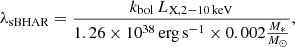 (1)
(1)
where kbol is a bolometric correction factor, which converts the 2 − 10 keV X-ray luminosity to AGN bolometric luminosity. For our sample, Lbol measurements are already available, as described earlier in this section, and thus a bolometric correction is not required. Nevertheless, we chose to use Eq. (1) for the calculation of λsBHAR, as it is the most common method used to calculate λsBHAR and it also facilitates a direct comparison with the SFRnorm − λsBHAR measurements of our previous studies (Mountrichas et al. 2021c, 2022b). For the same reasons, instead of the MBH measurements that are available for our sources, we chose to use the redshift-independent scaling relation between MBH and bulge mass, Mbulge, of Marconi & Hunt (2003), with the assumption that the Mbulge can be approximated by the M*. Specifically, we used MBH = 0.002 Mbulge. Finally, for kbol, we adopt the value of kbol = 25. This value is used in many studies (e.g., Elvis et al. 1994; Georgakakis et al. 2017; Aird et al. 2018; Mountrichas et al. 2021c, 2022b). Lower values have also be used (e.g., kbol = 22.4 in Yang et al. 2017), as well as luminosity-dependent bolometric corrections (e.g., Hopkins et al. 2007; Lusso et al. 2012). In Sect. 5.3.3, we examine how good these approximations are and their impact on the calculation of λsBHAR.
4. Final samples
In this section, we describe the criteria we apply to compile the final dataset of X-ray sources, drawn from the XMM-XXL catalogue (Sect. 2.1), and the final control sample of non-AGN galaxies, drawn from the VIPERS survey (Sect. 2.2).
4.1. The final X-ray dataset
We needed to use only sources (X-ray and non-AGN galaxies) that have the most reliable M* and SFR measurements. For that purpose, for the X-ray sources, we used the final sample presented in Mountrichas (2023). A detailed description of the photometric and reliability criteria that were applied is provided in Sect. 2.4 of that study. In brief, we require our sources to have measurements in the following photometric bands: u, g, r, i, z, J, H, K, W1, W2, and W4, where W1, W2, and W4 are the WISE photometric bands at 3.4, 4.6 and 22 μm. To exclude sources with bad SED fits and unreliable host galaxy measurements, a reduced χ2 threshold of  was imposed (e.g., Masoura et al. 2018; Buat et al. 2021). We also excluded systems for which CIGALE could not constrain the parameters of interest (SFR, M*). To this end, the two values that CIGALE provides for each estimated galaxy property are used. One value corresponds to the best model and the other (Bayesian) value is the likelihood-weighted mean value. A large difference between the two calculations suggests a complex likelihood distribution and important uncertainties. We therefore only include in our analysis sources with
 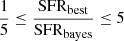 and
and 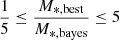 , where SFRbest and M*, best are the best-fit values of SFR and M*, respectively and SFRbayes and M∗,bayes are the Bayesian values estimated by CIGALE. 687 broad-line, X-ray AGN with spectroscopic redshifts meet the above requirements and also have available MBH measurements in the catalogue of Liu et al. (2016).
We then restricted the redshift range of the X-ray dataset to match that of the galaxy control sample (i.e., the VIPERS survey, 0.5 ≤ z ≤ 1.2). Altogether, 240 AGN meet this requirement. In Mountrichas et al. (2021c, 2022a,b), we found that the SFRnorm − LX relation depends on the M* range probed by the sources. Specifically a flat SFRnorm − LX relation was found for the least and most massive systems (log [M*(M⊙)] < 10.5 and log [M*(M⊙)] > 11.5), with SFRnorm ∼ 1. However, for intermediate stellar masses (10.5 < log [M*(M⊙)] < 11.5), the value of SFRnorm was found to be ≤1 at low-to-moderate LX (log[LX,2−10 keV(erg s−1)] < 44); whereas at higher LX, SFRnorm > 1 (e.g., see Fig. 5 in Mountrichas et al. 2022a). Therefore, in this study, we restricted the analysis to those sources with 10.5 < log [M*(M⊙)] < 11.5. Within this M* range, both of our datasets are also mass-complete (Davidzon et al. 2013; Mountrichas & Shankar 2023), as required for the calculation of SFRnorm.
Following previous studies that examined the impact of the AGN feedback on their host galaxies, by calculating SFRnorm using only star-forming systems (e.g., Mullaney et al. 2015; Masoura et al. 2018; Mountrichas et al. 2021c), we exclude quiescent (Q) systems from our sources. To identify Q galaxies, we used the distribution of the specific SFR  measurements of the galaxy control sample (e.g., similarly to Mountrichas et al. 2021c, 2022a,b). Mountrichas & Shankar (2023), applied this methodology on sources in the XMM-XXL field to classify galaxies as Q. From their subset of Q sources, 19 are among our 178 AGN. Their exclusion results in 159 X-ray systems. We note that the inclusion of the 19 AGN hosted by Q systems in our analysis does not affect our overall results and conclusions.
Since the galaxy control sample used in this study is smaller compared to those used in our previous works (see next section), we applied a final criterion to ensure that the SFRnorm calculations of each AGN that is included in our analysis are robust. That is to say, we only used AGN whose SFRnorm was calculated by matching the X-ray sources with at least 300 sources in the galaxy control sample. Increasing this threshold reduces significantly the size of the X-ray dataset; while at lower values, the scatter of our measurements is higher. A total of 122 X-ray AGN fulfill all the aforementioned criteria. Their LX and MBH values as a function of redshift are presented in Fig. 1.
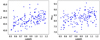 |
Fig. 1. LX (left panel) and MBH (right panel) as a function of redshift, for the 122 X-ray AGN used in our analysis. |
4.2. The final galaxy control sample
For the galaxy control sample, we apply the same photometric selection criteria and reliability requirements that we applied for the X-ray AGN sample. In addition, we excluded some sources that are included in the X-ray catalogue and we identified and rejected non-X-ray AGN systems. Specifically, we used the CIGALE measurements and excluded sources with fracAGN > 0.2, consistently with our previous studies (Mountrichas et al. 2021c, 2022a,b). Here, fracAGN is the fraction of the total IR emission coming from the AGN. This excludes ∼60% of the sources in the galaxy reference catalogue. This fraction is in line with our previous studies. A detailed analysis of the fracAGN criterion is provided in Sect. 3.3 in Mountrichas et al. (2022a). A total of 3622 galaxies fulfill all the aforementioned requirements. Finally, we excluded quiescent galaxies following the process described in the previous section. There are 3371 galaxies that remain and these are the sources in our control sample that we include in the analysis.
5. Results and discussion
In this section, we compare the SFR of AGN and non-AGN galaxies as a function of various black hole properties. Specifically, we study SFRnorm as a function of LX, MBH, nEdd, and λsBHAR. In Fig. 2, we present the four SMBH properties for the final X-ray dataset. We also apply three correlation statistics: one parametric (Pearson) and two non-parametric statistics (Spearman and Kendall) to quantify the correlations among them. The p-values are presented in Table 1. All parameters are strongly correlated with each other with the exception of the nedd − LX.
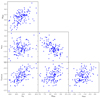 |
Fig. 2. Correlations among the four SMBH properties used in our study. Specifically, we present the correlations among the MBH, the LX, the specific black hole accretion rate |
p-values from the correlation analysis we apply for the four SMBH properties used in our analysis.
5.1. SFRnorm as a function of X-ray luminosity
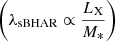
First, we examined SFRnorm as a function of LX. The results are shown in the top-left panel of Fig. 3. The small, blue circles present the measurements for individual AGN, while the large, red circles show the binned results. For the latter, the measurements are grouped in bins of LX of size 0.5 dex. The errors presented are 1σ errors, calculated via bootstrap resampling (e.g., Loh 2008). We find that the SFR of AGN is lower or at most equal to that of non-AGN galaxies (SFRnorm ≤ 1) at low and moderate LX (log[LX,2−10 keV(erg s−1)] ≤ 44) increases at higher LX, in agreement with previous studies (Mountrichas et al. 2021c, 2022a,b).
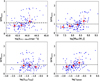 |
Fig. 3. SFRnorm as a function of SMBH properties. The SFRnorm parameter as a function of LX (top, left panel), MBH (top, right panel), Eddington ratio (bottom, left panel), and λsBHAR (bottom, right panel) are presented. |
The p-values from the three correlation statistics we use to calculate the correlation between SFRnorm and LX are presented in Table 2. The results indicate a strong correlation between the two parameters, independent of the statistical method applied.
p-values of correlation analysis, using sources with 0.5 ≤ z ≤ 1.2.
5.2. SFRnorm as a function of black hole mass
In a recent study, Piotrowska et al. (2022), analyzed three cosmological hydrodynamical simulations (Eagle, Illustris, and IllustrisTNG), by utilizing a random forest classification. They searched for the most effective parameter to separate star-forming and quenched galaxies in the Local Universe. They considered stellar mass, dark matter halo mass, black hole accretion rate, and black hole mass in their investigation. Their analysis showed that black hole mass was the most predictive parameter of galaxy quenching. Bluck et al. (2023), extended these results from the Local Universe to cosmic noon. These findings suggest that the cumulative impact of AGN feedback on a galaxy is encapsulated in the mass of the supermassive black hole and not in the X-ray luminosity, which is a proxy of the current accretion rate.
Hence, we chose to examine the SFRnorm as a function of black hole mass. Our goal is to examine if SFRnorm and MBH are correlated and compare their correlation with that between SFRnorm and LX. The top-right panel of Fig. 3 presents the SFRnorm as a function of MBH. The results show that SFRnorm increases with MBH on the full range of black hole masses spanned by our dataset. Specifically, in galaxies that host AGN with low MBH (log [MBH (M⊙)] < 8), their SFR is lower or equal to the SFR of non-AGN systems. Then, AGN with more massive black holes (log [MBH (M⊙)] > 8.5) reside in galaxies that cause their SFRs to be enhanced compared to non-AGN. The correlation analysis (Table 2) suggests a strong correlation between SFRnorm and MBH.
We also split our datasets into two redshift bins, using a threshold at z = 0.9 and repeat the correlation analysis. The choice of the redshift cut is twofold. Primarily, it aligns with the median redshift of the AGN sample. Furthermore, this redshift value corresponds to the redshift at which different spectral lines have been used for the calculation of MBH (see Sect. 3.3). The results are presented in Tables 3 and 4. The same trends are observed with those using sources in the full redshift interval, that is a strong correlation is found between SFRnorm and MBH in both redshift ranges. However, this correlation appears less strong in the lowest redshift interval compared to that found in the highest redshift bin. This could imply that the correlation between the two properties is, mainly, driven by massive MBH (MBH ≳ 108.5 M⊙) that are poorly detected at z < 0.9 in the dataset used in our analysis (Fig. 1). This interpretation is also supported by the strong correlation between LX and MBH (Fig. 2) combined with the results from previous studies that have shown that the SFRnorm − LX relation is nearly flat at LX < 1044 erg s−1 and shows a positive correlation only at higher LX (Mountrichas et al. 2021c, 2022a,b).
p-values of correlation analysis, using sources with 0.5 ≤ z ≤ 0.9.
p-values of correlation analysis, using sources with 0.5 < z ≤ 1.2.
A comparison of the p-values with those in the previous section, shows that the correlation between SFRnorm and MBH is similar to that between SFRnorm and LX. Subsequently, we explore whether this observation holds when considering the associated uncertainties of LX and MBH. For that purpose, we utilize the linmix module (Kelly 2007) that performs linear regression between two parameters, by repeatedly perturbing the datapoints within their uncertainties. The p-values obtained are 3.2 × 10⁻⁵ and 7.6 × 10⁻⁴ for the SFRnorm − LX and SFRnorm − MBH, respectively. These findings suggest, that despite accounting for uncertainties in LX and MBH measurements, there exists a robust correlation between these two properties and SFRnorm and that the two correlations are indeed similar.
As shown in Fig. 2 and Table 1, LX and MBH are strongly correlated. To investigate further the correlation among SFRnorm, LX and MBH, we perform a partial-correlation analysis (PCOR). PCOR measures the correlation between two variables while controlling for the effects of a third (e.g., Lanzuisi et al. 2017; Yang et al. 2017; Mountrichas et al. 2022b). We use one parametric statistic (Pearson) and one non-parametric statistic (Spearman). Table 5 lists the results of the p-values. Regardless of the parametric statistic of choice, p-values for the SFRnorm − MBH relation are smaller compared to the corresponding p-values for the SFRnorm − LX relation. This implies that the correlation between SFRnorm and MBH is more robust compared to that with LX, even when factoring in the existing correlation between MBH and LX. This deduction remains valid even when we partition the dataset into two redshift bins, specifically at z = 0.9.
p-values of partial correlation analysis, among SFRnorm, LX and MBH.
Mountrichas et al. (2022b) applied PCOR analysis on sources in the COSMOS field and found that SFRnorm is correlated stronger with M* than with LX. Yang et al. (2017) used galaxies in the CANDELS/GOODS-South field and examined the correlation between the black hole accretion rate (BHAR; which is measured directly from the LX), SFR and M*. They found that the BHAR is linked mainly to M* rather than SFR. There is also a well known correlation between the M* and the MBH (e.g., Merloni et al. 2010; Sun et al. 2015; Suh et al. 2020; Setoguchi et al. 2021; Poitevineau et al. 2023). Recently, Mountrichas (2023) reported such a correlation between MBH and M* using AGN in the XMM-XXL field, which is the same X-ray dataset used in this work. We applied a PCOR analysis, this time among SFRnorm, MBH, and M*. The results (presented in Table 6, top two lines) suggest that SFRnorm is linked more to MBH than M*. However, we note that for the reasons mentioned in Sect. 4, our datasets have been restricted to a relatively narrow M* range (10.5 < log [M*(M⊙)] < 11.5). Therefore, although the MBH parameter spans ∼2.5 orders of magnitude, that of M* spans only an order of magnitude among our samples.
p-values of partial correlation analysis, among SFRnorm, M*, and MBH.
To increase the M* range that our sources could probe, we lifted the M* requirement. There are 209 AGN and 4454 galaxies within 10 < log [M*(M⊙)] < 12. Using these two subsets, we calculated the SFRnorm for the 240 AGN and then we applied a PCOR analysis among SFRnorm, MBH and M*. The results are presented in the two bottom lines of Table 6. The p-values of the non-parametric statistic (Spearman) are similar; however, the p-value using the parametric statistic (Pearson) are lower for the SFRnorm − MBH, suggesting that the correlation between SFRnorm − MBH is stronger than the correlation between SFRnorm − M*. We note that these results should be taken with caution since our samples are not mass-complete in the full M* range that is considered in this exercise – and specifically within 10.0 < log [M*(M⊙)] < 10.5.
Overall, we conclude that SFRnorm is mostly linked to MBH rather than LX. Our results also suggest that the SFRnorm − M* correlation is due to the underlying M* − MBH. The picture that emerges corroborates the idea that the MBH is a more robust tracer of AGN feedback compared to the instantaneous activity of the SMBH – represented by LX – and as such MBH is a better predictive parameter of the changes of the SFR of the host galaxy, as theoretical studies have also suggested (Piotrowska et al. 2022; Bluck et al. 2023). Our results are also in line with the aforementioned studies regarding the negative AGN feedback they report, at least up to MBH ∼ 108.5 M⊙ (i.e., SFRnorm < 1). The increase in SFRnorm that we detect in our results suggests that this negative feedback may become less impactful on the SFR of the host galaxy, as we transition to systems with more massive SMBHs. These studies have additionally shown that the fraction of quenched galaxies increases with MBH. To investigate this claim, we would need to examine the fraction of quiescent systems as a function of MBH in our dataset. However, the small sample size used in our analysis and the low number of quiescent systems included do not allow for such an investigation.
5.3. SFRnorm as a function of Eddington ratio and specific black hole accretion rate
In this section, we investigate the correlation between SFRnorm and two other SMBH properties that represent the instantaneous AGN activity. Specifically, we study the relation between SFRnorm − nEdd and SFRnorm − λsBHAR. We also examine whether λsBHAR is a good proxy of the nEdd.
5.3.1. SFRnorm as a function of Eddington ratio
The Eddington ratio provides another important property of the SMBH. Setoguchi et al. (2021) used 85 moderately luminous (log Lbol ∼ 44.5 − 46.5 erg s−1) AGN from the Subaru/XMM-Newton Deep Field (SXDF) and found a strong correlation between the SFR of AGN and nEdd (correlation coefficient: r = 0.62). Recently, Georgantopoulos et al. (2023) studied the stellar populations of obscured and unobscured AGN at 0.6 < z < 1.0. Based on their analysis, the stellar age of both AGN types increases at lower Eddington ratio values (see the bottom-left panel of their Fig. 4 and top-right panel of their Fig. 11).
The bottom, left panel of Fig. 3, presents our calculations for SFRnorm as a function of the Eddington ratio. The value of SFRnorm remains roughly constant regardless of the value of nEdd. This is confirmed by the results of the correlation analysis, shown in Table 2 (see also Tables 3 and 4 for different redshift intervals). This nearly flat SFRnorm − nEdd relation can be explained by the correlations among the MBH, LX and nEdd, presented in Fig. 2. There is a strong anti-correlation between nEdd and MBH, but a positive correlation between nEdd and LX, while a strong positive correlation is detected between MBH and LX. We note that when we examine the relation between the SFR of AGN and nEdd, we find a (strong) correlation (r = 0.54), similar to that found by Setoguchi et al. (2021).
5.3.2. SFRnorm as a function of the specific black hole accretion rate
The specific black hole accretion rate is often used as a proxy of the Eddington ratio. Previous studies found an increase in the SFRnorm with λsBHAR (see Figs. 10 and 11 in Mountrichas et al. 2021c, 2022b, respectively). Pouliasis et al. (2022) used X-ray AGN in the COSMOS, XMM-XXL and eFEDS, at z > 3.5 and found that AGN that lie inside or above the main sequence (i.e., SFRnorm ≥ 1) exhibit higher λsBHAR values compared to X-ray sources that lie below the MS.
Our results, presented in the bottom- right panel of Fig. 3, agree with these previous findings. Specifically, we observe an increase in SFRnorm with λsBHAR. The application of a correlation analysis shows that there is a strong correlation between the two parameters, albeit not as strong as the correlation found between SFRnorm − LX and SFRnorm − MBH (Tables 2–4).
Mountrichas et al. (2022b) examined the correlation between SFRnorm and λsBHAR using X-ray sources in the COSMOS field and compared their results with those using AGN in the Boötes, presented in Mountrichas et al. (2021c) (see Fig. 11 and Table 5 in Mountrichas et al. 2022b). Although both datasets present a nearly, linear increase in the SFRnorm with LX, the amplitude of SFRnorm differs for the same λsBHAR values, for the two datasets. They attributed this difference to the different properties of the AGN from the two samples included in λsBHAR bins of the same value. Specifically, COSMOS sources are less luminous and less massive than their Boötes counterparts in λsBHAR bins of similar values. Therefore, if a dataset probes AGN within a large range of LX and M*, this could increase the scatter of SFRnorm for the same λsBHAR values, thus weakening the correlation between SFRnorm and λsBHAR and rendering λsBHAR useless as a parameter with respect to studying the impact of AGN feedback on the SFR of the host galaxy.
5.3.3. Considering λsBHAR as a good proxy for the Eddington ratio
As mentioned in the previous section, λsBHAR is often used as a proxy of nEdd on the basis that there is a linear relation between the M* and MBH and that Lbol can be inferred by LX. Prompted by the different relations found between SFRnorm − nEdd and SFRnorm − λsBHAR, we investigated this possibility further.
Lopez et al. (2023) used X-ray selected AGN in the miniJPAS footprint and found (among other aspects) that the Eddington ratio and λsBHAR have a difference of 0.6 dex. They attributed this difference to the scatter on the MBH − M* relation of their sources. The median value of nEdd of our sample, calculated using the Lbol measurements of CIGALE, is nEdd = −1.26, (nEdd = −1.33, using the values available in the Liu et al. 2016, catalogue). The median value of λsBHAR, estimated using Eq. (1), is λsBHAR = −1.08. Thus, we find a median difference of ∼0.25 between nEdd and λsBHAR. Although this difference is lower than that reported by Lopez et al. (2023), below we examine the cause of it.
We re-calculated λsBHAR, using the Lbol measurements from CIGALE (see Sect. 3.4) instead of the product of kbol LX. In this case, the median value of λsBHAR is −1.25. This value is in excellent agreement with that of nEdd (−1.26), using for the calculation of the latter the Lbol measurements from CIGALE. We also calculated λsBHAR keeping the same numerator as in Eq. (1), but using the MBH measurements available in our dataset instead of the MBH − M* scaling relation. In this case, the median difference between the distributions of λsBHAR and nEdd is ∼0.08. We note that for the sources used in our analysis, the scaling relation between MBH and M* is, MBH ≈ 0.003 M* (see also Sect. 3.3 in Mountrichas 2023), which is in good agreement with the MBH = 0.002 Mbulge used in Eq. (1).
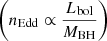
Therefore, the way Lbol is calculated seems to play an equally important role with the MBH − M* scaling relation on the comparison between nEdd and λsBHAR in our sample. The mean difference between the Lbol calculated by CIGALE and the product of kbolLX is 0.24 dex, with a dispersion of 0.35. CIGALE measurements suggest a mean kbol = 14.8 (i.e., a mean difference of zero for the two Lbol measurements). Finally, we compared the Lbol measurements of CIGALE with those using a luminosity dependent kbol. Specifically, we used the prescription of Lusso et al. (2012), using the values presented in their Table 2 for their spectroscopic type-1 AGN. In this case, the two calculations are in very good agreement with a mean difference of 0.04 dex and a dispersion of 0.34. Figure 4 presents the comparison between the Lbol measurements using the formula presented in Lusso et al. (2012) and CIGALE.
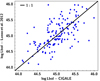 |
Fig. 4. Comparison of the Lbol calculations of CIGALE with the Lbol measurements using the formula derived in Lusso et al. (2012). The two measurements are in very good agreement with a mean difference of 0.04 dex. and a dispersion of 0.34. |
We conclude that caution has to be taken when λsBHAR is used as a proxy of nEdd, since the calculation of Lbol and the scatter in the MBH − M* scaling relation can cause (large) discrepancies between the estimated values of the two parameters.
6. Conclusions
We used 122 X-ray AGN in the XMM-XXL-N field and 3371 VIPERS galaxies, within the redshift and stellar mass ranges of 0.5 ≤ z ≤ 1.2 and 10.5 < log [M*(M⊙)] < 11.5, respectively. The X-ray sources probe luminosities within 43 < log[LX,2−10 keV(erg s−1)] < 45. Both populations meet strict photometric selection criteria and various selection requirements to ensure that only sources with robust (host) galaxy measurements are included in the analysis. The latter have been calculated via SED fitting, using the CIGALE code. Using these datasets, we calculated the SFRnorm parameter to compare the SFR of AGN with the SFR of non-AGN galaxies, as a function of various black hole properties. Specifically, we examined the correlations of SFRnorm with the LX, MBH, nEdd and λsBHAR. Our main results can be summarized as follows:
-
Those AGNs with low black hole masses (log (MBH/M*) < 8) have lower or at most equal SFR compared to that of non-AGN galaxies, while AGN with more massive black holes (log(MBH/M∗) > 8.5) tend to live in galaxies with (mildly) enhanced SFR compared to non-AGN systems.
-
The SFRnorm parameter is strongly correlated with both LX and MBH. However, the correlation between SFRnorm − MBH is stronger compared to the correlation between SFRnorm − LX. Our results also suggest that MBH drives the correlation between SFRnorm − M* that has been found in previous studies.
-
We do not detect a significant correlation between SFRnorm and Eddington ratio.
-
A correlation is found between SFRnorm and specific black hole accretion rate. However, this correlation is weaker compared to that between SFRnorm − LX and SFRnorm − MBH and its scatter may increase for samples that span a wide range of LX and M*.
-
The estimation of the AGN bolometric luminosity and the scatter of the MBH − M* scaling relation may cause discrepancies between the specific black hole accretion rate and the Eddington ratio measurements. Therefore, caution has to be taken when the former is used as a proxy for the latter.
These results suggest that there is a strong correlation between SFRnorm and AGN activity when the latter is represented by LX, λsBHAR, and MBH. A flat relation was only found between SFRnorm and nEdd, that can be interpreted as the net result of the different correlations (i.e., positive and negative) among nedd, MBH, and LX (Fig. 2). Based on our analysis, MBH is the most robust tracer of AGN feedback and the best predictive parameter of the changes of the SFR of the host galaxy.
Acknowledgments
This project has received funding from the European Union’s Horizon 2020 research and innovation program under grant agreement no. 101004168, the XMM2ATHENA project. The project has received funding from Excellence Initiative of Aix-Marseille University–AMIDEX, a French ‘Investissements d’Avenir’ programme. This work was partially funded by the ANID BASAL project FB210003. M.B. acknowledges support from FONDECYT regular grant 1211000. This research has made use of TOPCAT version 4.8 (Taylor 2005).
References
- Aird, J., Coil, A. L., & Georgakakis, A. 2018, MNRAS, 474, 1225 [NASA ADS] [CrossRef] [Google Scholar]
- Alexander, D. M., & Hickox, R. C. 2012, New Astron. Rev., 56, 93 [Google Scholar]
- Bernhard, E., Grimmett, L. P., Mullaney, J. R., et al. 2019, MNRAS, 483, L52 [NASA ADS] [CrossRef] [Google Scholar]
- Bluck, A. F. L., Piotrowska, J. M., & Maiolino, R. 2023, ApJ, 944, 108 [NASA ADS] [CrossRef] [Google Scholar]
- Boquien, M., Burgarella, D., Roehlly, Y., et al. 2019, A&A, 622, A103 [NASA ADS] [CrossRef] [EDP Sciences] [Google Scholar]
- Bower, R. G., Benson, A. J., & Crain, R. A. 2012, MNRAS, 422, 2816 [NASA ADS] [CrossRef] [Google Scholar]
- Boyle, B. J., Shanks, T., Croom, S. M., et al. 2000, MNRAS, 317, 1014 [NASA ADS] [CrossRef] [Google Scholar]
- Brown, A., Nayyeri, H., Cooray, A., et al. 2019, ApJ, 871, 87 [NASA ADS] [CrossRef] [Google Scholar]
- Bruzual, G., & Charlot, S. 2003, MNRAS, 344, 1000 [NASA ADS] [CrossRef] [Google Scholar]
- Buat, V., Ciesla, L., Boquien, M., Małek, K., & Burgarella, D. 2019, A&A, 632, A79 [NASA ADS] [CrossRef] [EDP Sciences] [Google Scholar]
- Buat, V., Mountrichas, G., Yang, G., et al. 2021, A&A, 654, A93 [NASA ADS] [CrossRef] [EDP Sciences] [Google Scholar]
- Charlot, S., & Fall, S. M. 2000, ApJ, 539, 718 [Google Scholar]
- Dale, D. A., Helou, G., Magdis, G. E., et al. 2014, ApJ, 784, 83 [Google Scholar]
- Davidzon, I., Bolzonella, M., Coupon, J., et al. 2013, A&A, 558, A23 [NASA ADS] [CrossRef] [EDP Sciences] [Google Scholar]
- Dubois, Y., Peirani, S., Pichon, C., et al. 2016, MNRAS, 463, 3948 [Google Scholar]
- Dunn, R. J. H., & Fabian, A. C. 2006, MNRAS, 373, 959 [Google Scholar]
- Elvis, M., Wilkes, B. J., McDowell, J. C., et al. 1994, ApJS, 95, 1 [Google Scholar]
- Ferrarese, L., & Merritt, D. 2000, ApJ, 539, 9 [Google Scholar]
- Florez, J., Jogee, S., Sherman, S., et al. 2020, MNRAS, 497, 3273 [NASA ADS] [CrossRef] [Google Scholar]
- Garilli, B., Guzzo, L., Scodeggio, M., et al. 2014, A&A, 562, A23 [NASA ADS] [CrossRef] [EDP Sciences] [Google Scholar]
- Georgakakis, A., Coil, A. L., Willmer, C. N. A., et al. 2011, MNRAS, 418, 2590 [NASA ADS] [CrossRef] [Google Scholar]
- Georgakakis, A., Salvato, M., Liu, Z., et al. 2017, MNRAS, 469, 3232 [NASA ADS] [CrossRef] [Google Scholar]
- Georgantopoulos, I., Pouliasis, E., Mountrichas, G., et al. 2023, A&A, 673, A67 [NASA ADS] [CrossRef] [EDP Sciences] [Google Scholar]
- Guzzo, L., Scodeggio, M., Garilli, B., et al. 2014, A&A, 566, A108 [NASA ADS] [CrossRef] [EDP Sciences] [Google Scholar]
- Häring, N., & Rix, H.-W. 2004, ApJ, 604, L89 [Google Scholar]
- Hopkins, P. F., Richards, G. T., & Hernquist, L. 2007, ApJ, 654, 731 [Google Scholar]
- Jahnke, K., Bongiorno, A., Brusa, M., et al. 2009, ApJ, 706, 215 [Google Scholar]
- Kelly, B. C. 2007, ApJ, 665, 1489 [Google Scholar]
- Komatsu, E., Smith, K. M., Dunkley, J., et al. 2011, ApJS, 192, 18 [Google Scholar]
- Koutoulidis, L., Mountrichas, G., Georgantopoulos, I., Pouliasis, E., & Plionis, M. 2022, A&A, 658, A35 [NASA ADS] [CrossRef] [EDP Sciences] [Google Scholar]
- Lanzuisi, G., Delvecchio, I., Berta, S., et al. 2017, A&A, 602, A13 [Google Scholar]
- Le Fèvre, O., Saisse, M., Mancini, D., et al. 2003, in Instrument Design and Performance for Optical/Infrared Ground-based Telescopes, eds. M. Iye, & A. F. M. Moorwood, SPIE Conf. Ser., 4841, 1670 [CrossRef] [Google Scholar]
- Liu, Z., Merloni, A., Georgakakis, A., et al. 2016, MNRAS, 459, 1602 [Google Scholar]
- Loh, J. M. 2008, ApJ, 681, 726 [CrossRef] [Google Scholar]
- Lopez, I. E., Brusa, M., Bonoli, S., et al. 2023, A&A, 672, A137 [NASA ADS] [CrossRef] [EDP Sciences] [Google Scholar]
- Lusso, E., Comastri, A., Simmons, B. D., et al. 2012, MNRAS, 425, 623 [Google Scholar]
- Magorrian, J., Tremaine, S., Richstone, D., et al. 1998, AJ, 115, 2285 [Google Scholar]
- Małek, K., Buat, V., Roehlly, Y., et al. 2018, A&A, 620, A50 [Google Scholar]
- Marconi, A., & Hunt, L. K. 2003, ApJ, 589, L21 [Google Scholar]
- Masoura, V. A., Mountrichas, G., Georgantopoulos, I., et al. 2018, A&A, 618, A31 [NASA ADS] [CrossRef] [EDP Sciences] [Google Scholar]
- Masoura, V. A., Mountrichas, G., Georgantopoulos, I., & Plionis, M. 2021, A&A, 646, A167 [EDP Sciences] [Google Scholar]
- McMahon, R. G., Banerji, M., Gonzalez, E., et al. 2013, The Messenger, 154, 35 [NASA ADS] [Google Scholar]
- Menzel, M.-L., Merloni, A., Georgakakis, A., et al. 2016, MNRAS, 457, 110 [Google Scholar]
- Merloni, A., Bongiorno, A., Bolzonella, M., et al. 2010, ApJ, 708, 137 [Google Scholar]
- Mountrichas, G. 2023, A&A, 672, A98 [NASA ADS] [CrossRef] [EDP Sciences] [Google Scholar]
- Mountrichas, G., & Shankar, F. 2023, MNRAS, 518, 2088 [Google Scholar]
- Mountrichas, G., Georgakakis, A., & Georgantopoulos, I. 2019, MNRAS, 483, 1374 [NASA ADS] [CrossRef] [Google Scholar]
- Mountrichas, G., Buat, V., Georgantopoulos, I., et al. 2021a, A&A, 653, A70 [NASA ADS] [CrossRef] [EDP Sciences] [Google Scholar]
- Mountrichas, G., Buat, V., Yang, G., et al. 2021b, A&A, 646, A29 [EDP Sciences] [Google Scholar]
- Mountrichas, G., Buat, V., Yang, G., et al. 2021c, A&A, 653, A74 [NASA ADS] [CrossRef] [EDP Sciences] [Google Scholar]
- Mountrichas, G., Buat, V., Yang, G., et al. 2022a, A&A, 663, A130 [NASA ADS] [CrossRef] [EDP Sciences] [Google Scholar]
- Mountrichas, G., Masoura, V. A., Xilouris, E. M., et al. 2022b, A&A, 661, A108 [NASA ADS] [CrossRef] [EDP Sciences] [Google Scholar]
- Mukai, K. 1993, Legacy, 3, 21 [Google Scholar]
- Mullaney, J. R., Alexander, D. M., Aird, J., et al. 2015, MNRAS, 453, L83 [Google Scholar]
- Park, T., Kashyap, V. L., Siemiginowska, A., et al. 2006, ApJ, 652, 610 [Google Scholar]
- Pierre, M., Pacaud, F., Adami, C., et al. 2016, A&A, 592, A1 [NASA ADS] [CrossRef] [EDP Sciences] [Google Scholar]
- Pineau, F. X., Derriere, S., Motch, C., et al. 2017, A&A, 597, A28 [NASA ADS] [CrossRef] [EDP Sciences] [Google Scholar]
- Piotrowska, J. M., Bluck, A. F. L., Maiolino, R., & Peng, Y. 2022, MNRAS, 512, 1052 [NASA ADS] [CrossRef] [Google Scholar]
- Poitevineau, R., Castignani, G., & Combes, F. 2023, A&A, 672, A164 [NASA ADS] [CrossRef] [EDP Sciences] [Google Scholar]
- Pouliasis, E., Mountrichas, G., Georgantopoulos, I., et al. 2020, MNRAS, 495, 1853 [NASA ADS] [CrossRef] [Google Scholar]
- Pouliasis, E., Mountrichas, G., Georgantopoulos, I., et al. 2022, A&A, 667, A56 [NASA ADS] [CrossRef] [EDP Sciences] [Google Scholar]
- Rosario, D. J., Trakhtenbrot, B., Lutz, D., et al. 2013, A&A, 560, A72 [NASA ADS] [CrossRef] [EDP Sciences] [Google Scholar]
- Santini, P., Rosario, D. J., Shao, L., et al. 2012, A&A, 540, A109 [NASA ADS] [CrossRef] [EDP Sciences] [Google Scholar]
- Scodeggio, M., Guzzo, L., Garilli, B., et al. 2018, A&A, 609, A84 [NASA ADS] [CrossRef] [EDP Sciences] [Google Scholar]
- Setoguchi, K., Ueda, Y., Toba, Y., & Akiyama, M. 2021, ApJ, 909, 188 [NASA ADS] [CrossRef] [Google Scholar]
- Shen, Y., & Liu, X. 2012, ApJ, 753, 125 [NASA ADS] [CrossRef] [Google Scholar]
- Shen, Y., Greene, J. E., Strauss, M. A., Richards, G. T., & Schneider, D. P. 2008, ApJ, 680, 169 [Google Scholar]
- Shen, Y., Richards, G. T., Strauss, M. A., et al. 2011, ApJS, 194, 45 [Google Scholar]
- Shen, Y., McBride, C. K., White, M., et al. 2013, ApJ, 778, 98 [Google Scholar]
- Shimizu, T. T., Mushotzky, R. F., Meléndez, M., Koss, M., & Rosario, D. J. 2015, MNRAS, 452, 1841 [NASA ADS] [CrossRef] [Google Scholar]
- Shimizu, T. T., Mushotzky, R. F., Meléndez, M., et al. 2017, MNRAS, 466, 3161 [NASA ADS] [CrossRef] [Google Scholar]
- Sobral, D., Smail, I., Best, P. N., et al. 2013, MNRAS, 428, 1128 [NASA ADS] [CrossRef] [Google Scholar]
- Stalevski, M., Fritz, J., Baes, M., Nakos, T., & Popović, L. Č. 2012, MNRAS, 420, 2756 [Google Scholar]
- Stalevski, M., Ricci, C., Ueda, Y., et al. 2016, MNRAS, 458, 2288 [Google Scholar]
- Stanley, F., Harrison, C. M., Alexander, D. M., et al. 2015, MNRAS, 453, 591 [Google Scholar]
- Sun, M., Trump, J. R., Brandt, W. N., et al. 2015, ApJ, 802, 14 [NASA ADS] [CrossRef] [Google Scholar]
- Suh, H., Civano, F., Trakhtenbrot, B., et al. 2020, ApJ, 889, 32 [NASA ADS] [CrossRef] [Google Scholar]
- Sutherland, W., & Saunders, W. 1992, MNRAS, 259, 413 [Google Scholar]
- Taylor, M. B. 2005, in Astronomical Data Analysis Software and Systems XIV, eds. P. Shopbell, M. Britton, & R. Ebert, ASP Conf. Ser., 347, 29 [Google Scholar]
- Tremaine, S., Gebhardt, K., Bender, R., et al. 2002, ApJ, 574, 740 [NASA ADS] [CrossRef] [Google Scholar]
- Villa-Velez, J. A., Buat, V., Theule, P., Boquien, M., & Burgarella, D. 2021, A&A, 654, A153 [NASA ADS] [CrossRef] [EDP Sciences] [Google Scholar]
- Wright, E. L., Eisenhardt, P. R. M., Mainzer, A. K., et al. 2010, AJ, 140, 1868 [Google Scholar]
- Yang, G., Chen, C. T. J., Vito, F., et al. 2017, ApJ, 842, 72 [NASA ADS] [CrossRef] [Google Scholar]
- Yang, G., Boquien, M., Buat, V., et al. 2020, MNRAS, 491, 740 [Google Scholar]
- Yang, G., Boquien, M., Brandt, W. N., et al. 2022, ApJ, 927, 192 [NASA ADS] [CrossRef] [Google Scholar]
All Tables
p-values from the correlation analysis we apply for the four SMBH properties used in our analysis.
All Figures
|
Fig. 1. LX (left panel) and MBH (right panel) as a function of redshift, for the 122 X-ray AGN used in our analysis. |
| In the text | |
|
Fig. 2. Correlations among the four SMBH properties used in our study. Specifically, we present the correlations among the MBH, the LX, the specific black hole accretion rate |
| In the text | |
|
Fig. 3. SFRnorm as a function of SMBH properties. The SFRnorm parameter as a function of LX (top, left panel), MBH (top, right panel), Eddington ratio (bottom, left panel), and λsBHAR (bottom, right panel) are presented. |
| In the text | |
|
Fig. 4. Comparison of the Lbol calculations of CIGALE with the Lbol measurements using the formula derived in Lusso et al. (2012). The two measurements are in very good agreement with a mean difference of 0.04 dex. and a dispersion of 0.34. |
| In the text | |
Current usage metrics show cumulative count of Article Views (full-text article views including HTML views, PDF and ePub downloads, according to the available data) and Abstracts Views on Vision4Press platform.
Data correspond to usage on the plateform after 2015. The current usage metrics is available 48-96 hours after online publication and is updated daily on week days.
Initial download of the metrics may take a while.