| Issue |
A&A
Volume 635, March 2020
|
|
|---|---|---|
| Article Number | A104 | |
| Number of page(s) | 28 | |
| Section | Stellar structure and evolution | |
| DOI | https://doi.org/10.1051/0004-6361/201937189 | |
| Published online | 16 March 2020 | |
A high-precision abundance analysis of the nuclear benchmark star HD 20⋆,⋆⋆
1
Astronomisches Rechen-Institut, Zentrum für Astronomie der Universität Heidelberg, Mönchhofstr. 12-14, 69120 Heidelberg, Germany
e-mail: mhanke@ari.uni-heidelberg.de
2
Max Planck Institute for Astronomy, Königstuhl 17, 69117 Heidelberg, Germany
3
Landessternwarte, Zentrum für Astronomie der Universität Heidelberg, Königstuhl 12, 69117 Heidelberg, Germany
4
INAF – Osservatorio Astronomico d’Abruzzo, Via M. Maggini snc, Teramo, Italy
5
INFN – Sezione di Perugia, Via A. Pascoli snc, Perugia, Italy
6
Carnegie Observatories, 813 Santa Barbara St., Pasadena, CA 91101, USA
Received:
26
November
2019
Accepted:
31
January
2020
Metal-poor stars with detailed information available about their chemical inventory pose powerful empirical benchmarks for nuclear astrophysics. Here we present our spectroscopic chemical abundance investigation of the metal-poor ([Fe/H] = −1.60 ± 0.03 dex), r-process-enriched ([Eu/Fe] = 0.73 ± 0.10 dex) halo star HD 20, using novel and archival high-resolution data at outstanding signal-to-noise ratios (up to ∼1000 Å−1). By combining one of the first asteroseismic gravity measurements in the metal-poor regime from a TESS light curve with the spectroscopic analysis of iron lines under non-local thermodynamic equilibrium conditions, we derived a set of highly accurate and precise stellar parameters. These allowed us to delineate a reliable chemical pattern that is comprised of solid detections of 48 elements, including 28 neutron-capture elements. Hence, we establish HD 20 among the few benchmark stars that have nearly complete patterns and low systematic dependencies on the stellar parameters. Our light-element (Z ≤ 30) abundances are representative of other, similarly metal-poor stars in the Galactic halo that exhibit contributions from core-collapse supernovae of type II. In the realm of the neutron-capture elements, our comparison to the scaled solar r-pattern shows that the lighter neutron-capture elements (Z ≲ 60) are poorly matched. In particular, we find imprints of the weak r-process acting at low metallicities. Nonetheless, by comparing our detailed abundances to the observed metal-poor star BD +17 3248, we find a persistent residual pattern involving mainly the elements Sr, Y, Zr, Ba, and La. These are indicative of enrichment contributions from the s-process and we show that mixing with material from predicted yields of massive, rotating AGB stars at low metallicity improves the fit considerably. Based on a solar ratio of heavy- to light-s elements – which is at odds with model predictions for the i-process – and a missing clear residual pattern with respect to other stars with claimed contributions from this process, we refute (strong) contributions from such astrophysical sites providing intermediate neutron densities. Finally, nuclear cosmochronology is used to tie our detection of the radioactive element Th to an age estimate for HD 20 of 11.0 ± 3.8 Gyr.
Key words: stars: abundances / stars: chemically peculiar / stars: individual: HD 20 / stars: evolution / Galaxy: halo / nuclear reactions / nucleosynthesis / abundances
Full Table C.1 is only available at the CDS via anonymous ftp to cdsarc.u-strasbg.fr (130.79.128.5) or via http://cdsarc.u-strasbg.fr/viz-bin/cat/J/A+A/635/A104
© ESO 2020
1. Introduction
Studies of metal-poor stars as bearers of fossil records of Galactic evolution are among the cornerstones of Galactic archeology. In this respect, revealing the kinematics and chemistry of this relatively rare subclass of stars provides vital insights into the build-up of galaxy components, such as the Galactic halo and the origin of chemical elements.
The nucleosynthesis of iron-peak elements, from Si to approximately Zn (atomic numbers 14 ≤ Z ≤ 30), is thought to be dominated by explosive nucleosynthesis from both thermonuclear supernovae (Type Ia exploding white dwarfs) and core-collapse supernovae (CCSNe, massive stars). On the other hand, the major production of elements from Li up to and including Si is thought to be dominated by hydrostatic burning processes (Woosley & Weaver 1995; Nomoto et al. 2006; Kobayashi et al. 2019).
Beyond the iron peak, electrostatic Coulomb repulsion ensures that charged-particle reactions play a minuscule role in element synthesis (with the possible exception of proton-rich nuclei). Temperatures high enough for charged particles to overcome the Coulomb barrier photo-dissociate the larger nuclei. Thus, most of the elements heavier than the iron peak result from neutron captures, which are divided into the slow (s) and rapid (r) processes by their capture rates with respect to the β-decay timescale (Burbidge et al. 1957; Cameron 1957). The involved neutron densities differ by many orders of magnitude and are thought to be n < 108 cm−3 and n ≳ 1020 cm−3 for the s- and r-process, respectively (Busso et al. 2001; Meyer 1994). In recent years, an additional, so-called intermediate (i) process – representing neutron densities in between typical r- and s-values – is gaining attention as models are capable of reproducing some peculiar chemical patterns typically found in C-rich metal-poor stars (e.g., Roederer et al. 2016; Hampel et al. 2016, 2019; Koch et al. 2019).
The main s-process is believed to be active during the thermally pulsing phases of asymptotic giant branch (AGB) stars, which provide the required low neutron fluxes (e.g., Gallino et al. 1998; Straniero et al. 2006; Lugaro et al. 2012; Karakas & Lattanzio 2014), whereas several sites have been proposed to generate neutron-rich environments for the r-process to occur. Viable candidates are neutrino-driven winds in CCSNe (Arcones et al. 2007; Wanajo 2013), jets in magneto-rotational supernovae (MR SNe, Cameron 2003; Mösta et al. 2018), and neutron star mergers (NSMs, e.g., Lattimer & Schramm 1974; Chornock et al. 2017). The latter site recently gained a lot of attention since, for example, Pian et al. (2017) found indications for short-lived r-process isotopes in the spectrum of the electromagnetic afterglow of the gravitational wave event GW170817 that was detected and confirmed as an NSM by the LIGO experiment (Abbott et al. 2017). The authors, however, could not single out any individual elements. Only later, direct spectroscopic investigations revealed the newly produced neutron-capture element Sr in this NSM (Watson et al. 2019). Nonetheless, as stressed by, for instance, Côté et al. (2019) and Ji et al. (2019), other sites like MR SNe may still be needed to explain the full budget of r-process elements observed in the Galaxy. Nuclear benchmark stars allow for detailed studies of each of the neutron-capture processes.
From an observational point of view, there have been a number of spectroscopic campaigns that specifically targeted metal-poor stars to constrain the nucleosynthesis of heavy elements in the early Milky Way, among which are, to name a few, Beers & Christlieb (2005), Hansen et al. (2012, 2014), and the works by the r-process alliance (e.g., Hansen et al. 2018a; Sakari et al. 2018, and follow-up investigations). Following Beers & Christlieb (2005), the rare class of r-process-rich stars is commonly subdivided by a somewhat arbitrary cut into groups of moderately enhanced r-I (0.3 ≤ [Eu/Fe]1 ≤ +1.0 dex; [Ba/Eu] < 0 dex) and strongly enhanced r-II ([Eu/Fe] > +1.0 dex; [Ba/Eu] < 0 dex) stars. In the context of this classification, our benchmark star HD 20 falls in the r-I category. Recently, Gull et al. (2018) reported on the first finding of an r-I star with a combined “r + s” pattern, which was explained by postulating mass transfer from a companion that evolved through the AGB phase.
Here we present a comprehensive spectroscopic abundance analysis of HD 20, an r-process-rich star at the peak of the halo metallicity distribution function ([Fe/H] = −1.60 dex) with a heavy-element pattern that suggests pollution with s-process material.
Based on the full 6D phase-space information from the second data release (DR2) of the Gaia mission (Gaia Collaboration 2018), Roederer et al. (2018a) concluded that HD 20 may be chemodynamically associated with two other metal-poor halo stars with observed r-process excess. Based on its kinematics – characterized by a highly eccentric orbit ( ) and a close pericentric passage (
 kpc) – and its low metallicity, the authors speculate that HD 20 and its associates may have been accreted from a disrupted satellite.
Among others, HD 20 has been a subject of two previous abundance studies by Burris et al. (2000) and Barklem et al. (2005) who reported eight and ten abundances for elements with Z ≥ 30, respectively. Both groups employed medium-resolution (R = λ/FWHM ∼ 20 000) spectra at signal-to-noise ratios (S/N) slightly above 100 pixel−1. Table 1 lists the findings for the eight elements that are in common between both works and we note systematic disagreements – in a sense that the abundances by Burris et al. (2000) generally are above Barklem et al. (2005) – exceeding even the considerable quoted errors of about 0.2 dex. The authors adopted very similar effective temperatures (Teff) for their analyses (5475 K versus 5445 K), while the employed stellar surface gravities (log g) and microturbulent velocities (vmic) differ strongly by +0.41 dex and −0.30 km s−1. Inconsistencies between the studies are likely to be tied to these discrepancies as has already been recognized by Barklem et al. (2005, see also Appendix B.2 for a detailed discussion of the impact of model parameters on individual stellar abundances).
Comparison of abundances for HD 20 in common between Burris et al. (2000) and Barklem et al. (2005).
Our work is aimed at painting a complete picture of the chemical pattern in HD 20 consisting of 58 species from the primordial light element Li to the heavy r-process element U. To this end, a compilation of high-quality, newly obtained and archival spectra was used, allowing for many elemental detections with high internal precisions. Furthermore, specific attention was devoted to the determination of accurate stellar parameters in order to mitigate the effect of systematic error contributions to the robustness of the deduced pattern. In this respect, an essential building block of our analysis is a highly accurate and precise stellar surface gravity from an asteroseismic analysis of the light curve that was obtained by NASA’s Transiting Exoplanet Survey Satellite (TESS, Ricker et al. 2015). Hence, we established HD 20 as a new metal-poor benchmark star – both in terms of fundamental properties as well as complete abundance patterns – which, in light of its bright nature (V ≈ 9 mag), provides an ideal calibrator for future spectroscopic surveys.
This paper is organized as follows: in Sect. 2, we introduce the spectroscopic, photometric, and astrometric data sets employed throughout the analyses. Section 3 is dedicated to the detailed discussion of our derived stellar parameters, followed by Sect. 4, which presents a description of the adopted procedures for the abundance analysis. Our results for HD 20 and constraints drawn from its abundance pattern can be found in Sect. 5. Finally, in Sect. 6, we summarize our findings and provide an outlook for further studies.
2. Observations and data reduction
2.1. Spectroscopic observations
We obtained a spectrum of HD 20 in the night of August 15, 2013 using both arms of the Magellan Inamori Kyocera Echelle (MIKE) spectrograph (Bernstein et al. 2003). An exposure of 1093 s integration time was taken using a slit width of 0.5″ and a 2 × 1 on-chip-binning readout mode. This setup allowed for a full wavelength coverage from 3325 to 9160 Å at a resolution of R ≈ 45 000.
The raw science frame was reduced by means of the pipeline reduction package by Kelson (2003), which performs flat-field division, sky modeling and subtraction, order tracing, optimal extraction, and wavelength calibration based on frames obtained with the built-in ThAr lamp. For the MIKE red spectrum, the reduction routine combined 26 ten-second “milky flat” exposures, taken using a quartz lamp and diffuser, resulting in a S/N of approximately 100 per 2 × 1 binned CCD pixel near the middle of the array, per exposure. This gave a total S/N of about 500 pixel−1 in the combined flat. Due to lower flux in the blue quartz lamp, the milky flat exposure time was set to 20 s per frame. In addition, the 26 blue-side milky flat exposures were supplemented with seven ten-second exposures of a hot star, HR 7790, taken with the diffuser. The median seeing of 0.72″, corresponding to 5.4 CCD pixels FWHM, indicates that the flux for each wavelength point was taken from approximately 2 FWHM, or about 11 pixels. At the Hα wavelength the pixels are 0.047 Å wide, indicating roughly 21 pixels per Å. These details suggest that the S/N of the final, extracted, flat field flux is 5000 to 7000 Å−1, significantly greater than the S/N of the stellar spectrum. The resulting S/N of the extracted object spectrum ranges from about 40 Å−1 at the blue-most edge to more than 1200 Å−1 redward of 7000 Å. We present the detailed distribution of S/N with wavelength in Fig. 1.
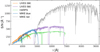 |
Fig. 1. S/N as a function of wavelength for the employed spectra of HD 20 from all three high-resolution spectrographs. Since the dispersion spacing between adjacent pixels varies among the instruments, we present the S/N per 1 Å. |
Our MIKE observation was complemented by data retrieved through the ESO Advanced Data Products (ADP) query form, with two additional, reduced high-resolution spectra for this star: The first is a 119 s, reduced exposure (ID 090.B-0605(A)) from the night of October 13, 2012 using the UVES spectrograph with a dichroic (Dekker et al. 2000) at the ESO/VLT Paranal Observatory. For the blue arm, a setup with an effective resolution of R ∼ 58 600 centered at a wavelength of 390 nm (UVES 390) was chosen, whereas the red arm was operated at R ∼ 66 300 with a central wavelength of 580 nm (UVES 580). Especially the UVES 390 exposure poses an additional asset, since it supersedes our MIKE spectrum in the UV at higher S/N and – more importantly – bluer wavelength coverage and considerably higher resolution.
The second ESO spectrum was taken on December 29, 2006 (ID 60.A-9036(A)) employing the HARPS spectrograph (Mayor et al. 2003) at the 3.6 m Telescope at the ESO La Silla Observatory. With a similar wavelength coverage and at substantially lower S/N than the UVES spectra, this observation adds a very high resolution of 115 000 that was used to corroborate our findings for the intrinsic line broadening (Sect. 3.5). The S/N values reached with both ESO spectrographs are shown in Fig. 1 alongside the distribution for MIKE.
2.2. Radial velocities and binarity
All spectra were shifted to the stellar rest frame after determining radial velocities through cross correlation with a synthetic template spectrum of parameters that are representative for HD 20 (see Sect. 3 and Table 2). For the HARPS and UVES spectra, we established the radial velocity zero point using standard stars that were observed in the same nights (HD 69830 and HD 7041, respectively, with reference values from Soubiran et al. 2018), whereas we used the telluric O2 B-band at ∼6900 Å to calibrate the MIKE spectrum. This way, we found vhelio = −57.16 ± 0.15, −57.04 ± 0.26, and −56.86 ± 0.44 km s−1 from the HARPS, UVES, and MIKE spectra of HD 20. These findings are consistent with the mean value −57.18 ± 0.11 km s−1 from the radial-velocity monitoring program by Carney et al. (2003) and considerably above the reported value by Hansen et al. (2015) of −57.914 ± 0.041 km s−1. A graphical juxtaposition is shown in Fig. 2. We note that – owing to the usage of different spectrographs and resolutions – our radial velocity analysis is by no means homogeneous and slight discrepancies are therefore to be expected. Nevertheless, the observed offset with respect to Hansen et al. (2015) is significant. The anomaly with respect to Carney et al. (2003) has already been noted by Hansen et al. (2015) and was linked to a difference in the applied scales. Apart from this systematic bias, over a time span of 10 011 days, there is no indication of real radial velocity variations. As a consequence, a binary nature of HD 20 can be ruled out with high confidence.
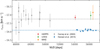 |
Fig. 2. Comparison of literature time series for vhelio by Carney et al. (2003, gray-filled circles) and Hansen et al. (2015, blue-filled circles) to measurements from the three spectra employed throughout this study (see legend). The gray and blue dashed lines resemble the median values for the two reference samples. |
Fundamental properties and stellar parameters entering this work.
2.3. Photometry and astrometric information
Visual to near-infrared broadband photometric information for HD 20 was compiled from the literature and is listed in Table 2 together with the respective errors and sources. BVRCIC photometry was presented in Beers et al. (2007) in a program that was targeting specific stars such as HD 20. Their results were also employed by Barklem et al. (2005) and follow-up works by relying on the deduced parameters. The authors report V = 9.236 ± 0.001 mag, which is in strong disagreement to other findings in the literature. For example, the HIPPARCOS catalog (ESA 1997) lists V = 9.04 mag (used for temperature estimates in the spectroscopic studies of Gratton et al. 2000; Fulbright & Johnson 2003), while Anthony-Twarog & Twarog (1994) provide a consistent value of V = 9.059 ± 0.013 mag (used, e.g., by Carney et al. 2003). Furthermore, we estimate V ≈ 9.00 ± 0.05 mag from Gaia photometry and the analytical relation for (G − V) as a function of GBP and GRP2. For completeness, we ought to mention the finding of V = 9.40 mag by Ducati (2002), which again poses a strong deviation. We point out that HD 20 does not exhibit any signs of photometric variability as revealed by time-resolved photometry over 6.6 yr from DR9 of the All-Sky Automated Survey for Supernovae (ASAS-SN, Jayasinghe et al. 2019) showing – which is again in agreement with most of the literature – V = 9.01 ± 0.08 mag.
Despite the relatively low quoted internal uncertainties, we discard the photometry by Beers et al. (2007) and Ducati (2002) from consideration as we suspect inaccuracies in the calibration procedures. A disruptive factor might be a blend contribution by a star about 14″ to the southeast, although we deem this an unlikely option since Gaia DR2 reports it to be much fainter (G = 8.849 mag versus 14.675 mag). Consequently, we resorted to magnitudes for the B-band from the Tycho-2 catalog (Høg et al. 2000) and for V by Anthony-Twarog & Twarog (1994). For the near-infrared JHKs photometry we queried the 2MASS catalog (Skrutskie et al. 2006) and the Strömgren color b − y is taken from Hauck & Mermilliod (1998).
In terms of reddening we applied E(B − V) = 0.0149 ± 0.0005 mag, which was extracted from the reddening maps by Schlafly & Finkbeiner (2011). Whenever dereddened colors or extinction-corrected magnitudes were employed, we adopted the optical extinction ratio RV = A(V)/E(B − V) = 3.1 attributed to the low-density interstellar medium (ISM) together with the reddening ratios E(color)/E(B − V) compiled in Table 1 of Ramírez & Meléndez (2005). Considering the overall very low reddening of HD 20, uncertainties in the latter ratios ought to have negligible impact on the quantities deduced from photometry.
A parallax of ϖ = 1.945 ± 0.053 mas was retrieved from Gaia DR2 from which we computed a geometric distance to HD 20 of d = 507 ± 13 pc3. Here we accounted for the quasar-based parallax zero point for Gaia DR2 of −0.029 mas (Lindegren et al. 2018). Our finding is fully in line with the distance  pc derived in the Bayesian framework of Bailer-Jones et al. (2018).
3. Stellar parameters
A crucial part of any spectroscopic analysis which is aimed at high-accuracy chemical abundances is the careful determination of the stellar parameters entering the model atmospheres needed when solving for the radiative transfer equations. Here we outline the inference method applied for determining the parameters; effective temperature, surface gravity, microturbulence, metallicity, and line broadening.
Our adopted stellar parameters (Table 2) are based on a spectroscopic analysis of Fe lines that were corrected for departures from the assumption of local thermodynamic equilibrium (LTE) together with asteroseismic information from the TESS mission, whereas several other techniques – both spectroscopic and photometric – including their caveats are discussed in Appendix A.
3.1. Surface gravity from TESS asteroseismology
Recently, Creevey et al. (2019) showed in their time-resolved radial velocity analysis of the benchmark star HD 122563 that the asteroseismic scaling relation
based on the frequency fmax of maximum power of solar-like oscillations holds even in the regime of metal-poor and evolved stars. This motivated the exploration of the feasibility of an asteroseismic gravity determination for HD 20.
Fortunately, TESS measured a 27.4 days light curve with a two-minute cadence for this star during Sector 2. We employed the lightkurve Python package (Lightkurve Collaboration 2018) to retrieve and reduce the data in order to calculate the power spectrum seen in Fig. 3. A power excess is identifiable around the frequency fmax ≈ 27 μHz, which we attribute to solar-like oscillations.
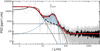 |
Fig. 3. Power spectral density (PSD) for HD 20 based on TESS light-curve data. The thick black line depicts a smoothed version of the PSD (thin gray line) and the best-fit model is shown in red. The blue shaded area indicates the power excess, whereas individual model components are represented by thin blue and black dashed lines. |
We performed a fit to the obtained power spectrum following the prescriptions by Campante et al. (2019). Therefore, we assumed a multi-component background model consisting of super-Lorentzian profiles that account for various granulation effects (see, e.g., Corsaro et al. 2017, for details) as well as a constant noise component. The decision on the number of super-Lorentzian components for the background was made based on Bayesian model comparison using Bayes factors from evidences that were estimated with the Background4 extension to the high-DImensional And multi-MOdal NesteD Sampling (DIAMONDS5, Corsaro & De Ridder 2014) algorithm. We found that a model with three super-Lorentzian components has an insignificantly stronger support compared to a two-component one. The latter observation indicates that – given the data – the meso-granulation around frequencies of fmax/3 ≈ 9 μHz is indistinguishable from the component due to super-granulation and/or other low-frequency signals since they occupy a similar frequency range in HD 20. Thus, we adopted only two super-Lorentzians for the background fit. Finally, a Gaussian profile was used to represent the power excess on top of the background model.
In order to sample and optimize the high-dimensional parameter space of all involved model coefficients, we again made use of DIAMONDS. The resulting best-fit model, as well as its individual components, are depicted in Fig. 3. We estimated  μHz which translates into
  dex from Eq. (1) using fmax, ⊙ = 3050 μHZ (Kjeldsen & Bedding 1995) and our adopted Teff. Owing to a weak coupling of the asteroseismic gravity to the temperature, we do not consider it in isolation, but refer the reader to Sect. 3.4, where we outline the procedure to reach simultaneous parameter convergence.
3.2. Iron lines
A list of suitable Fe I and Fe II lines for the purpose of deriving accurate stellar parameters was compiled using the Atomic Spectra Database (Kramida et al. 2018) of the National Institute of Standards and Technology (NIST). To this end, in order to mitigate biases by uncertain oscillator strengths (log gf), only those lines were considered that are reported to have measured log gf values with accuracy levels ≤10% (grade B or better in the NIST evaluation scheme) for Fe I and ≤25% (grade C or better) for Fe II lines. The lines retrieved this way were checked to be isolated by means of spectrum synthesis (see Sect. 4.1) and their EW was measured by EWCODE (Sect. 4.2). From these, we added the ones that were measured with more than 5σ significance to the final list. Laboratory line strengths for the resulting 133 Fe I transitions were measured and reported by Fuhr et al. (1988), O’Brian et al. (1991), Bard et al. (1991), and Bard & Kock (1994). For the 13 Fe II lines that survived the cleaning procedure, the data are taken from Schnabel et al. (2004).
3.3. Spectroscopic model atmosphere parameters
Throughout our analyses, we employed the LTE radiation transfer code MOOG (Sneden 1973, July 2017 release) including an additional scattering term in the source function as described by Sobeck et al. (2011)6. Our atmosphere models are based on the grid of 1D, static, and plane parallel ATLAS9 atmospheres by Castelli & Kurucz (2003) with opacity distribution functions that account for α-enhancements ([α/Fe] = +0.4, Sect. 5.3). Models for parameters between the grid points were constructed via interpolation in the grid. Here we used the iron abundance [Fe/H] as proxy for the models’ overall metallicities [M/H] since we assume that all elements other than the α-elements follow the solar elemental distribution scaled by [Fe/H]. We note that the fact that HD 20 shows enhancements in the neutron-capture elements (Sect. 5.4) does not prevent this assumption, as the elements in question are only detectable in trace amounts with negligible impact on atmospheric properties such as temperature, density, and gas or electron pressure.
Our Teff estimate is based on the spectroscopic excitation balance of Fe I lines. This technique relies on tuning the model temperature such that lines at different lower excitation potential (χex) yield the same abundance – in other words a zero-slope of log ϵ(Fe I) with χex is enforced. In this respect it is important to account for the circumstance that Fe I transitions are prone to substantial non-LTE (NLTE) effects in metal-poor stars, in a sense that not only the overall abundance is shifted toward higher values, but the magnitude of the effect varies with χex, too. Hence, as pointed out by Lind et al. (2012), the Teff for which the excitation trend is leveled is shifted to systematically offset temperatures from the LTE case (see Fig. 4). To overcome this problem, we computed NLTE abundance departures by interpolation in a close-meshed, precomputed grid of corrections that was created specifically for this project and parameter space (priv. comm.: M. Bergemann & M. Kovalev, see Bergemann et al. 2012a; Lind et al. 2012, for details).
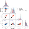 |
Fig. 4. Samples drawn from the posterior distribution of the stellar parameters (Eq. (2)). Shown are the three different approaches M1 (gray), M2 (red), and M3 (blue) with the darkness of the colors illustrating the local density as estimated from a Gaussian kernel density estimate. The sample sizes are 2 × 10⁴ and the adopted stellar parameters from method M3 (Tables 2 and 3) based on the median of the distributions are indicated using horizontal and vertical dashed lines. The correlation coefficients for pairs of two parameters in M3 are presented in the top left corner of each panel. The marginalized, one-dimensional distributions for the individual parameters are depicted by smoothed histograms at the top of each column. |
The microturbulence parameter vmic is an ad-hoc parameter that approximatively accounts for the effects of otherwise neglected turbulent motions in the atmosphere, which mainly affect the theoretical line strength of strong lines. Here we tuned vmic in order to erase trends of the inferred, NLTE-corrected abundances for Fe I features with the reduced line strength, RW = log (EW/λ).
Even though we prefer our highly accurate asteroseismic measurement over requiring spectroscopic ionization balance for determining log g, we discuss this method here to compare our findings to more classical spectroscopic parameter estimation methods that are widely used throughout the literature. The procedure is based on balancing abundances of neutral lines and singly ionized lines that are sensitive to changes in gravity (see also Appendix B.2). Hence, by tuning the model gravity to erase discrepancies between the abundances deduced from both ionization states of the same element, log g can be inferred. Commonly, especially for FGK stars, the high number of available Fe lines in both ionization stages qualifies this species as an ideal indicator. While the modeling of Fe II line strengths is insensitive to departures from LTE (< 0.01 dex), trustworthy gravities from the ionization balance can only be obtained once departures from LTE are removed from the Fe I abundances (e.g., Lind et al. 2012). In particular, by neglecting NLTE influences, one would considerably underestimate log ϵ(Fe I) and consequently log g. This can be seen in Fig. 5, where we compare Fe I under the LTE assumption to NLTE-corrected Fe I. Illustrated is the best abundance agreement – that is, a perfect overlap of both the log ϵ(Fe I)NLTE and log ϵ(Fe II)LTE7 abundance distributions – obtained for log g = 2.24 dex and [M/H] = −1.65 dex.
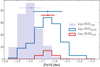 |
Fig. 5. Diagnostic plot for spectroscopic ionization balance. Shown are the histograms of the Fe abundance distributions ([Fe/H] = log ϵ(Fe) − 7.50 dex) at the adopted gravity (log g = 2.24 dex from method M2, see Sect. 3.4) both in LTE (gray filled) and NLTE (blue) for Fe I and in LTE for Fe II (red). NLTE corrections for Fe II remain well below 0.01 dex and are therefore neglected here. Points with error bars and arbitrary ordinate offsets at the top of the panel denote the means and standard deviations for each of the distributions of the same color. |
When assessing the error budget on [Fe/H], we caution that in this study’s realm of very high S/N spectra, random noise is not the prevailing origin for the line-by-line scatter of 0.10 dex and 0.03 dex for log ϵ(Fe I)NLTE and log ϵ(Fe II)LTE, respectively. In fact, looking at the abundance errors for individual lines from EW errors only (Table C.1), the random component remains well below 0.03 dex in the majority of cases. We conclude that the scatter is mostly of non-stochastic nature – for example due to uncertain oscillator strengths and flaws in the 1D assumption – and hence a division of the rms scatter by the square root of the number of lines is not a statistically meaningful quantifier of the metallicity error (see Appendix B.1 for more detailed discussions).
3.4. Bayesian inference
We emphasize that spectroscopic stellar parameters are strongly interdependent, that is, uncertainties and systematic errors of one quantity should not be considered in isolation. The usage of asteroseismic information mitigates this circumstance only to some degree as we show below. Hence, all model parameters need to be iterated until simultaneous convergence is reached. For this purpose, we used the emcee (Foreman-Mackey et al. 2013) Python implementation of a Markov chain Monte Carlo (MCMC) sampler in order to draw samples from the posterior probability distribution P of the four model parameters Teff, [M/H], log g, and vmic,

with ℒ being the likelihood function and p the prior. Here y denotes the measured EWs and x represents the set of model atmosphere parameters. A flat prior of unity was assumed within the parameter space covered by our grid of NLTE corrections, and zero otherwise. We explored three different likelihoods representing the purely spectroscopic LTE (M1) and NLTE (M2) methods, as well as a mixed “NLTE + asteroseismology” (M3) approach. The likelihoods take the form of
![$$ \begin{aligned} {\cal L} = \exp \left( { - \frac{{a_{{\chi _{{\rm{ex}}}}}^2}}{{2\sigma _a^2}} - \frac{{b_{{\rm{RW}}}^2}}{{2\sigma _b^2}} - \frac{{\Delta _{[{\rm{M/H],Fe}}\,{\rm{II}}}^2\,}}{{2\sigma _{{\rm{ Fe}}\,{\rm{II}}}^2}} - {\Gamma _i}} \right), \end{aligned} $$](/articles/aa/full_html/2020/03/aa37189-19/aa37189-19-eq16.gif)
where aχex and bRW are the slopes of the deduced LTE (M1) or NLTE (M2 and M3) abundances, log ϵFe I(y, x, χex), with χex and RW for any given set of parameters x. The variances of the latter slopes were determined from repeated linear fits to bootstrapped samples by means of robust least squares involving a smooth L1 loss function. We prefer this non-parametric approach over ordinary least squares because of the systematically underestimated abundance errors from EW uncertainties alone (see previous section). The third term in Eq. (3) represents the difference between the model metallicity and Fe II abundance, whereas Γi introduces the gravity sensitivity. For approaches M1 and M2, it represents the ionization (im-)balance,
in the LTE and NLTE case, while we do not enforce ionization balance for M3, but use the asteroseismic information through
In this expression log gseis. is calculated from Eq. (1). We emphasize that, while being clearly subject to biases in LTE, a perfect ionization balance may not be desirable even in the 1D NLTE case (M2), because it still lacks proper descriptions of hydrodynamical and 3D conditions. These might pose other sources for differences between abundances from Fe I and Fe II at the true log g. In fact, there is a remaining marginal ionization imbalance log ϵFe II − log ϵFe I = 0.08 ± 0.10 when adopting the M3 approach.
Figure 4 shows various representations of the multidimensional posterior distributions for M1, M2, and M3. As expected, we found strong correlations between Teff, [M/H], and log g in the purely spectroscopically informed methods M1 and M2. Using approach M3, we can effectively lift the degeneracies with log g as quantified by insignificant Pearson correlation coefficients (Fig. 4). For each approach, we deduced the optimal parameters and error margins from the median, 15.9th, and 84.1th percentiles, respectively. These are listed in Table 3. It is evident that M1 significantly underestimates both [M/H] and log g due to deducing lower Fe I abundances that have a direct impact on the ionization balance and therefore the inferred gravity. M2 and M3, however, yield results that are in good agreement with the strongest deviation amounting to just 1.2σ in log g. This highlights the importance of considering NLTE effects already at the stage of stellar parameter inference and shows that 1D NLTE ionization balance is capable of producing gravities that are as accurate as the highly trustworthy asteroseismic scaling relations. Since the precision of the latter is better by about a factor of five, we adopt the parameters inferred from M3 throughout this work. We corroborated this set of fundamental stellar parameters using several independent techniques, including temperatures from the shapes of the Balmer lines in HD 20’s spectrum. We refer the reader to Appendix A for a detailed outline and comparison.
Median values and 68.2% confidence intervals for the stellar parameters from the posterior distributions for the three different likelihood functions (see main text for details).
3.5. Line broadening
Carney et al. (2003) report a rotational velocity of vrot sin i = 5.9 km s−1 for HD 20, which is unexpectedly high given the evolutionary state of this star where any initial rotation is expected to be eliminated. The authors caution, however, that the face value just below their instrumental resolution of 8.5 km s−1 might be biased due to a number of systematic influences on their method, amongst which is turbulent broadening (see also, e.g., Preston et al. 2019). Turbulent and rotational broadening have almost identical impacts on the line shape, a degeneracy that can only be broken using spectra of very high resolution and S/N (Carney et al. 2008). Hence – despite the name – we consider vrot sin i a general broadening parameter.
Given that rotation or any other line broadening mechanism are key quantities that critically affect the precision and accuracy of abundances from spectrum synthesis (Sect. 4), we tackled this property from a theoretical point of view. To this end, a collection of isolated Ti I and Ti II features were simulated using LTE radiative transfer in a CO5BOLD model atmosphere (Freytag et al. 2012), which realistically models the microphysics of stellar atmospheres under 3D, hydrodynamical conditions. We note that the chosen atmospheric parameters (Teff = 5500 K, log g = 2.5 dex, [M/H] = −2.0 dex) only roughly match our findings – hence deviations in the abundance scales can be expected. The overall line-shape, however, is expected to be reasonably accurately reproduced. Our synthetic profiles were compared to their observed counterparts in the UVES 580 spectrum, which offers the best trade-off between resolution and S/N in the considered wavelength regimes. The nominal velocity resolution is 4.5 km s−1. Comparisons for two representative lines are presented in Fig. 6. The 3D profiles are shown next to rotationally broadened, 1D versions and we find that no additional rotational broadening is required in the 3D case as the line shape can be fully recovered by properly accounting for microphysics together with the instrumental resolution. Thus, we conclude that – if at all – HD 20 is rotating only slowly (i.e., v sin i ≲ 1 km s−1). On top of the overall line broadening, slight profile asymmetries are correctly reproduced by the 3D models.
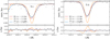 |
Fig. 6. Comparison of synthetic line shapes against the observed profiles in the UVES 580 spectrum for two representative Ti lines. Red spectra resemble 3D syntheses, while blue and orange colors indicate 1D syntheses with and without additional broadening. The instrumental profile (R = 66 230) was mimicked by convolution with a Gaussian kernel for all three types of synthesis. No rotational broadening was applied to the 3D syntheses. |
In order to improve our 1D spectrum syntheses beyond broadening by the instrumental line spread function, we analyzed the deviation of individual, isolated Fe features from their 1D LTE line shape. The comparison was performed against the UVES 580 and the HARPS spectrum. Based on 171 lines in common for both spectra, we found that a broadening velocity of vmac = 5.82 ± 0.03 km s−1 can successfully mimic the line shape from both spectrographs. The latter value is in good agreement with the value 5.9 km s−1 found by Carney et al. (2003), who do not list an error specific to HD 20 but quote general standard errors between 0.5 and 3 km s−1 for their entire sample of stars.
3.6. Other structural parameters
Given our spectroscopic temperature and metallicity, we can deduce HD 20’s luminosity through
![$$ \begin{aligned} \frac{L}{L_\odot } = \left(\frac{d}{10\,\mathrm{pc} }\right)^2 \frac{L_0}{L_\odot }\times 10^{-0.4\left(V - A(V) + \mathrm{BC}_V(T_\mathrm{eff} , \mathrm{[Fe/H]} )\right)} \end{aligned} $$](/articles/aa/full_html/2020/03/aa37189-19/aa37189-19-eq31.gif)
with the zero-point luminosity L0 (see Table 2) and the bolometric correction BCV from the calibration relation by Alonso et al. (1999a, henceforth AAM99), which itself depends on Teff and [Fe/H]. We find  , in line with the value 58.6 ± 2.2 reported in Gaia DR2. The error on L was computed through a Monte Carlo error propagation assuming Gaussian error distributions for the input variables and an additional uncertainty for BCV of 0.05 mag. The asymmetric error limits stem from the 15.9 and 84.1 percentiles of the final parameter distributions, respectively.
We can furthermore infer the stellar radius using
resulting in  . This compares to
  from Gaia DR2, where the slight discrepancy can be explained by a higher temperature estimate from Gaia (see discussion in Appendix A.1.3).
Finally, it is possible to deduce a mass estimate using the basic stellar structure equation
The solar reference values involved can be found in Table 2. As for Eq. (6), the bolometric magnitude Mbol can be computed from the V-band photometry and the BCV relation by AAM99. We find a mass of (0.76 ± 0.08) M⊙.
4. Abundance analysis
The abundances presented here were computed using either EWs (Sect. 4.2) or spectrum synthesis for such cases where blending was found to be substantial. For this purpose we employed the spectra providing the highest S/N at any given wavelength, that is, UVES 390 blueward of ∼4300 Å, MIKE blue for 4300 ≲ λ ≲ 5000 Å, and MIKE red in the regime 5000 ≲ λ ≲ 8000 Å (cf. Fig. 1). Despite the circumstance that MIKE reaches substantially more redward, we do not consider it there because of considerable fringing. The radiation transfer was solved using MOOG and an ATLAS9 model for our exact specifications (previous sections and Table 2) that was constructed via interpolation. Our computations involved molecular equilibrium computations involving a network consisting of the species H2, CH, NH, OH, C2, CN, CO, N2, NO, O2, TiO, H2O, and CO2. Individual, line-by-line abundances can be found in Table C.1, while we summarize the adopted final abundances and their associated errors in Table 4. In order to reduce the impact of outliers, abundances were averaged using the median. For ensembles of four and more lines, we computed the corresponding errors via the median absolute deviation (mad) which is scaled by the factor 1.48 in order to be conform with Gaussian standard errors. As noted already in Sect. 3.3, for the vast majority of species, the magnitude of the line-by-line scatter is inconsistent with merely the propagation of random spectrum noise, but accounts for additional – possibly systematic – sources of error further down in the abundance analysis. Consequently, we set a floor uncertainty of 0.10 dex for those species with less than four available lines, where the mad would not be a robust estimator for the scatter. For a discussion of this as well as of influences from uncertain stellar parameters, we refer the reader to Appendices B.1 and B.2. For elements with only one line measured with the line abundance uncertainty alone exceeding the floor error, we adopted the error on the line abundance instead.
Final adopted abundances.
4.1. Line list
Suitable lines for an abundance analysis of HD 20 were compiled and identified using atomic data from the literature. We retrieved all line data that are available through the Vienna Atomic Line Database (VALD, Piskunov et al. 1995; Ryabchikova et al. 2015) in the wavelength range from 3280 Å to 8000 Å, representing the combined wavelength coverage of the spectra at hand. In a first run, we synthesized a spectrum from this line list and discarded all profiles that did not exceed a line depth of 0.1% of the continuum level. The remaining features were visually checked for their degree of isolation and usability by comparing the observed spectra with syntheses with varying elemental abundances. The resulting list with the adopted line parameters and original sources thereof can be found in Table C.1. Additional hyperfine structure (HFS) line lists were considered for the elements Li (Hobbs et al. 1999), Sc (Kurucz & Bell 1995), V (Lawler et al. 2014), Mn (Den Hartog et al. 2011), Co (Kurucz & Bell 1995), Cu (Kurucz & Bell 1995), Ag (Hansen et al. 2012), Ba (McWilliam 1998), La (Lawler et al. 2001a), Pr (Sneden et al. 2009), Eu (Lawler et al. 2001b), Tb (Lawler et al. 2001c), Ho (Lawler et al. 2004), Yb (Sneden et al. 2009), and Lu (Lawler et al. 2009).
4.2. Equivalent widths
The majority of the spectral features identified to be suitable for our analysis are sufficiently isolated so that an EW analysis could be pursued. We measured EWs from the spectra of all three spectrographs using our own semi-automated Python tool EWCODE (Hanke et al. 2017). In brief, EWCODE places a local, linear continuum estimate that is based on the neighboring wavelength ranges next to the profile of interest and fits Gaussian profiles. The user is prompted with the fit and can interactively improve the fit by, for example, introducing additional blends or refining the widths of the continuum ranges. Our measurements for individual lines along with EWCODE’s error estimates are listed in Table C.1.
4.3. Notes on individual elements
In the following, we comment in detail on the analysis of abundances from several features that needed special attention exceeding the standard EW or spectrum synthesis analysis. Furthermore, whenever available, we comment on NLTE corrections that were applied to the LTE abundances.
4.3.1. Lithium (Z = 3)
The expected strongest feature of Li I is the resonance transition at 6707.8 Å. Despite our high-quality data, within the noise boundaries, the spectrum of HD 20 appears perfectly flat with no feature identifiable whatsoever. For the region in question we estimate from our MIKE spectrum S/N ≈ 1050 pixel−1, which would allow for 3σ detections of Gaussian-like features with EWs of at least 0.3 mÅ as deduced from the formalism provided in Battaglia et al. (2008). The latter EW translates into an upper limit log ϵ(Li) < −0.34 dex.
4.3.2. Carbon, nitrogen, and oxygen (Z = 6, 7, and 8)
Our C abundances are based on synthesis of the region around the CH G-band at ∼4300 Å with molecular line data for 12CH and 13CH from Masseron et al. (2014). We identified a range between 4310.8 Å and 4312.1 Å that in HD 20 is almost devoid of atomic absorption and hence is ideal for CH synthesis irrespective of other elemental abundances. We show this range in Fig. 7. Only very substantial changes in the model isotopic ratio 12C/13C have a notable effect on this region, manifesting mostly in an effective blue- or redshift of the molecular features. In contrast, the two 13CH profiles near ∼4230 Å (left panel of Fig. 7) are rather sensitive to the isotopic ratio. As cautioned by Spite et al. (2006), the blueward profile has a dominant blend they attribute to an unidentified transition from an r-process element. Given the r-process-rich nature of our star, we do not consider this feature here. Employing both ranges, one for the C abundance and one for 12C/13C, the two measures can be effectively decoupled as can be seen in Fig. 8, where we present the results of an MCMC sampling run used to draw from the posterior distribution of the fitted parameters in the regions indicated in Fig. 7. From this distribution we determine  . Though nominally less, an error of 0.05 dex was adopted for log ϵ(C) = 6.25 dex in order to account for the circumstance that the continuum level in the right-hand spectrum had to be established from a region more than one Å away on either side, thus introducing a slight normalization uncertainty.
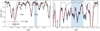 |
Fig. 7. C abundance and 12C/13C from the CH G-band in the UVES 390 spectrum. Left panel: region around the two features that are dominated by 13CH, one of which is used to pinpoint 12C/13C (blue rectangle). The bluer feature at ∼4230 Å was not considered due to an unidentified blend (see main text). The observed spectrum is represented by black dots connected by gray lines and the best-fit synthesis (red) and its abundance error margin of 0.05 dex are depicted in blue, respectively. The dashed spectrum shows a synthesis without any C. Right panel: same as left panel but in the range used to constrain the C (CH) abundance. |
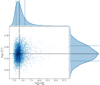 |
Fig. 8. Two-dimensional representation of the MCMC sample used to fit log ϵ(C) and 12C/13C simultaneously including the marginal distributions. Median values and asymmetric limits are displayed by dashed lines. |
We determined the N abundance in a similar fashion employing the NH-band at ∼3360 Å (see Fig. 9). From our synthesis we inferred log ϵ(N) = 6.21 ± 0.10 dex. The present data do not permit the determination of the isotopic ratio 14N/15N.
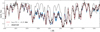 |
Fig. 9. Same as right panel of Fig. 7, but for a synthesis of the NH-band at ∼3360 Å. A synthesis without any N is indicated by the black dashed curve. The blue error range corresponds to an abundance variation of ±0.10 dex. |
Unfortunately, the frequently used [O I] line at 6300.3 Å is strongly blended with telluric absorption features in all available spectra and hence rendered useless for precise abundance studies. Nonetheless, the high S/N of the MIKE spectra allowed for the measurement of the much weaker [O I] transitions at 5577.3 Å and 6363.8 Å, from which we deduced a mean abundance of log ϵ(O I)LTE = 7.79 ± 0.18 dex, or [O/Fe] = 0.70 dex. The forbidden lines ought to have negligible LTE corrections, because they have metastable upper levels. Hence, the collisional rate is higher than the radiative rate and LTE is obtained, in other words log ϵ(O I)NLTE = log ϵ(O I)LTE. Severe changes in the O abundance result in non-negligible effects on the molecular equilibrium, in particular through their impact on the formation of CO. For this reason, the overabundance found here was considered in all syntheses, including the ones for CH and NH outlined above.
We note here that abundances from the O triplet at ∼7773 Å could be firmly detected and are listed in Table C.1. However, we discard them (log ϵ(O I)LTE ≈ 8.22 dex) from consideration in this work, since they are in strong disagreement to the abundances from the forbidden lines. The formation of the lines in question is subject to considerable NLTE effects as shown by, for example, Sitnova et al. (2013). Using the MPIA NLTE spectrum tools8 to retrieve corrections for individual line abundances, we found an average 1D NLTE bias of −0.14 dex, which is not enough to erase the discrepancy. We therefore suspect much stronger effects when considering line formation in NLTE using 3D dynamical models (e.g., Amarsi et al. 2019).
4.3.3. Sodium (Z = 11)
Equivalent widths from the two weak Na lines at 5682 Å and 5688 Å were employed to compute an abundance of log ϵ(Na)LTE = 4.50 ± 0.10 dex. We emphasize the artificial increase of the latter uncertainty to 0.10 dex as discussed earlier. According to the INSPECT database9 (Lind et al. 2011), for these lines and HD 20’s parameters a mean NLTE correction of −0.08 dex should be applied, leading to log ϵ(Na)NLTE = 4.42 dex and consequently [Na/Fe] = −0.14 dex. The frequently used Na I transitions at 6154 Å and 6160 Å could not be firmly detected in any of our spectra owing to HD 20’s rather high temperature, which strongly reduces the strength of these lines.
4.3.4. Magnesium (Z = 12)
The three Mg I lines employed for abundance determinations in this work were corrected for departures from the LTE assumptions by means of the MPIA NLTE spectrum tools, which is based on Bergemann et al. (2017a,b). The mean correction is only +0.04 dex, indicating that the effects are not severe for the selected lines.
4.3.5. Aluminum (Z = 13)
Our Al abundance for HD 20 is based on five neutral transitions. While spectrum syntheses revealed the 3944 Å profile to be severely blended, the other strong UV resonance feature at 3961 Å was found to be sufficiently isolated for getting a robust abundance. In addition, the high S/N of our MIKE spectrum allowed for the detection of two pairs of weak, high-excitation lines at ∼6697 Å and ∼7835 Å, respectively. In LTE, there is a considerable difference of almost 1 dex between the abundances from the resonance line (log ϵ(Al)LTE = 3.58 dex), and the four weak lines (log ϵ(Al)LTE = 4.54 dex). As shown by Nordlander & Lind (2017), this can be explained by substantial NLTE effects on Al line formation in metal-poor giants like HD 20. Indeed, by interpolation in their pre-computed grid, we found corrections of 1.02 dex for the strong line and 0.14 to 0.20 dex for the weak lines, which alleviates the observed discrepancy. We emphasize that [Al/Fe] (Table 4) remains unaltered by going from LTE to NLTE, because both the Fe I transitions and the majority of our Al I lines experience the same direction and magnitude of corrections. We note here that Barklem et al. (2005) report on a strong depletion in LTE of [Al/Fe] = −0.80 dex (on the scale of Asplund et al. 2009) based on the UV resonance line, only. Hence, that finding at face value should be treated with caution since severe NLTE biases can be expected.
4.3.6. Silicon (Z = 14)
Five of our 16 Si I lines with measured EWs have a correspondence in the MPIA NLTE database (Bergemann et al. 2013). The deduced corrections for HD 20’s stellar parameters are marginal at a level of −0.01 to −0.04 dex. As a consequence, the ionization imbalance of −0.28 dex between Si I and Si II that prevails in LTE cannot be compensated this way. Lacking NLTE corrections for our two Si II transitions, however, we cannot draw definite conclusions at this point.
4.3.7. Sulfur (Z = 16)
We detected in total four S features that are spread over two wavelength windows at ∼4695 Å and ∼6757 Å, corresponding to the second and eighth S I multiplet. Using spectrum synthesis, we found a mean abundance log ϵ(S I)LTE = 6.03 ± 0.04 dex that is mainly driven by the strongest profile at 4694.1 Å. Concerning influences of NLTE on S I, in the literature there is no study dealing with the second multiplet. For the eighth multiplet, however, Korotin (2008, 2009) and Korotin et al. (2017) showed that the expected corrections for HD 20 are minor and remain well below 0.10 dex. Since we detected no considerable difference in our LTE analysis between the eighth and second multiplet, we conclude that the correction – if any – for the second multiplet is probably small, too.
4.3.8. Potassium (Z = 19)
The K abundance presented here is based on the EWs of two red resonance lines at 7665 Å and 7699 Å, respectively. These lines are expected to be subject to severe departures from LTE. Mucciarelli et al. (2017) showed for giants in four globular clusters that the magnitude of the NLTE correction strongly increases with increasing Teff, log g, and log ϵ(K)LTE. One of their clusters, NGC 6752, exhibits a similar metallicity (−1.55 dex) as HD 20 and we estimate from their Fig. 3 a correction of our LTE abundance of at least −0.5 to −0.6 dex. For our adopted NLTE abundance (Table 4) we assume a shift by −0.55 dex.
4.3.9. Titanium (Z = 22)
Our LTE analysis of Ti lines shows an ionization imbalance of log ϵ(Ti I) − log ϵ(Ti II)LTE = −0.33 dex. We have determined line-by-line NLTE corrections for our Ti I abundances from the grid by Bergemann (2011) amounting to values ranging from +0.4 to +0.6 dex. It is noteworthy that corrections to Ti II are insignificant in the present regime of stellar parameters (cf., Bergemann 2011). The newly derived NLTE abundances switch the sign of the ionization imbalance with a reduced amplitude ((log ϵ(Ti I) − log ϵ(Ti II))NLTE = +0.14 dex). Inconsistencies in other metal-poor stars manifesting themselves in ionization imbalances even in NLTE have already been noted by Bergemann (2011) and were explained by inaccurate or missing atomic data. More recently, Sitnova et al. (2016) found lower NLTE corrections and therefore weaker – but still non-zero – ionization imbalances for stars in common with Bergemann (2011), which they mainly attributed to the inclusion of high-excitation levels of Ti I in their model atom. In light of prevailing uncertainties of Ti I NLTE calculations, we do not believe that the ionization imbalance of Ti contradicts our results from Sect. 3.3.
4.3.10. Manganese (Z = 25)
Following Bergemann & Gehren (2008), our four abundances from Mn I lines should experience a considerable mean NLTE adjustment of +0.40 dex and thus are consistent with a solar [Mn/Fe]. More recently, Mishenina et al. (2015) casted some doubt on the robustness of the aforementioned NLTE calculations by showing the absence of systematic discrepancies in LTE between multiplets that according to Bergemann & Gehren (2008) ought to have different NLTE corrections. Nonetheless, Bergemann et al. (2019) corroborated the strong NLTE corrections found in the earlier study. Moreover, the authors remark that Mn I transitions at a lower excitation potential of more than 2 eV are not strongly affected by convection – that is 3D effects – and are recommended as 1D NLTE estimator. Since the latter is satisfied for all of our four used Mn lines, our 1D NLTE abundance ought to be an accurate estimate.
4.3.11. Cobalt (Z = 27)
The Co NLTE corrections were obtained from Bergemann et al. (2010). For three out of the six measured lines corrections are available and amount to +0.46 dex on average.
4.3.12. Copper (Z = 29)
We measured three profiles of Cu I in our spectra, two of which originate from low-excitation (∼1.5 eV) states. Albeit for dwarfs, at [Fe/H] ∼ −1.5 dex, Yan et al. (2015) predicted for these two transitions at 5105.5 Å and 5782.2 Å stronger NLTE corrections compared to the ones for our high-excitation (∼3.8 eV) line. This is somewhat reflected in our LTE abundances where the lower-excitation lines yield a lower value by about 0.3 dex. Lacking a published pre-computed grid, it is hard to predict the exact amount of NLTE departures for our giant star and its temperature. Yet, Shi et al. (2018) and Korotin et al. (2018) showed that the corrections correlate much stronger with [Fe/H] than they do with log g or Teff. We make no attempt to rectify our Cu abundances at this point, but judging from the literature we note that the corrections are probably on the order of +0.2 dex for the low-excitation- and +0.1 dex for the high-excitation lines.
4.3.13. Strontium (Z = 38)
In principle, our spectra cover the UV resonance lines of Sr II at 4077 Å and 4215 Å, although we found those to be strongly saturated and we could not reproduce the line shape through LTE synthesis. Furthermore, the lines in question are subject to a substantial degree of blending by several atomic and molecular transitions (see also Andrievsky et al. 2011). Fortunately, it was possible to measure EWs of the much weaker lines at 4607 Å (Sr I) and at 4161 Å (Sr II). For these we deduced abundances of 1.00 dex and 1.50 dex, respectively, which indicates a substantial discrepancy between the two ionization stages. The latter can be attributed to considerable NLTE departures for the neutral transition. Bergemann et al. (2012b)10 and Hansen et al. (2013) performed extensive NLTE calculations for this line from which we extract a correction of +0.4 dex for HD 20’s stellar parameters. Thus, the observed difference is effectively erased, although we emphasize the lack of published Sr II corrections for the line and stellar parameters in question, which, in turn, may re-introduce a slight disagreement.
4.3.14. Zirconium (Z = 40)
Two out of our five measured Zr II lines were investigated for NLTE effects by Velichko et al. (2010). The authors note that departures mainly depend on metallicity and gravity, whereas there is only a weak coupling to Teff. From their published grid of corrections we extrapolate corrections of 0.15 dex and 0.18 dex for our abundances from the lines at 4209.0 Å and 5112.3 Å, respectively.
4.3.15. Barium (Z = 56)
In HD 20, the Ba II profile at 4554 Å is strongly saturated and thus largely insensitive to abundance. We further excluded the 6141 Å line because of blending by an Fe feature. Our abundance hence is based on synthesis of the two clean and only moderately strong transitions at 5853 Å and 6496 Å, yielding log ϵ(Ba II))LTE = 0.77 dex and 1.09 dex, respectively. In light of the recent work on NLTE line formation by Mashonkina & Belyaev (2019), the presented disagreement can be expected in LTE, as in our parameter regime NLTE corrections for the two lines differ. Indeed, interpolation in their published grid11 resulted in corrections of −0.10 dex and −0.27 dex, hence reducing the gap to 0.15 dex, which can be explained by the combined statistical uncertainties.
4.3.16. Lutetium (Z = 71)
The very high S/N of about 1000 pixel−1 in the MIKE spectrum together with an overall high Lu abundance ([Lu/Fe] = 0.93 dex) allowed for a solid detection (4.7 mÅ) of the otherwise very weak Lu II profile at 6221.9 Å. We mention the line here explicitly because it was found to have an exceptionally pronounced HFS structure, as we show in Fig. 10 where two syntheses are compared; one including HFS and one neglecting it. The line components were taken from Lawler et al. (2009). We note that we consider only the 175Lu isotope here, because the only other stable isotope, 176Lu, is expected to be a minority component judging from its solar fractional abundance (2.59%, Lawler et al. 2009). Despite the considerable additional line broadening due to atmospheric effects (Sect. 3.5), hyperfine splitting is still the dominant source of broadening, thus highlighting the importance of including it in our analysis.
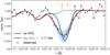 |
Fig. 10. Synthesis of the Lu II line at 6221.9 Å. The red line represents the best abundance match with an error of 0.1 dex (blue shaded region). The broad range of HFS components for 175Lu from Lawler et al. (2009) are indicated by vertical orange lines at the top and have been taken into account for this synthesis. The impact of the negligence of HFS on the line shape is indicated by the blue line. |
4.3.17. Upper limits on rubidium, lead, and uranium (Z = 37, 82, and 92)
For Rb, Pb, and U, it was not possible to obtain solid detections despite the high-quality spectra at hand. Nonetheless, we could estimate reasonable upper limits based on the lines at 7800.3 Å (Rb I), 4057.8 Å (Pb I), and 3859.6 Å (U II). Since there is a considerable amount of blending by a variety of species involved in shaping the spectrum in the three wavelength regimes, we cannot estimate the upper limit in the same way as for Li (Sect. 4.3.1). Thus, we used synthesis at varying abundances of the target elements in order to establish the highest abundance that is still consistent with the noise level present in the spectral regions (Figs. 11–13). This way, we found log ϵ(Rb) < 1.52 dex, log ϵ(Pb) < 0.37 dex, and log ϵ(U) < −1.21 dex, respectively.
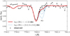 |
Fig. 11. Upper limit on Rb from the Rb I line at 7800.3 Å. The red model denotes the adopted upper limit of +1.52 dex, whereas blue lines are syntheses with Rb abundances successively increased by 0.2 dex. |
5. Results and discussion
5.1. Light elements (Z ≤ 8)
Our Li, C, and N abundances show evidence of a pattern that is commonly attributed to internal mixing occuring when a star reaches the RGB bump where processed material from the H-burning shell gets dredged up to the convective layer. Observationally, the effect can be seen in the stellar surface abundances of bright giants (brighter than the RGB-bump at log L/L⊙ ∼ 1.8; e.g., Gratton et al. 2000) and horizontal branch stars that show non-detections of Li and depletions of [C/Fe] in lockstep with low 12C/13C ratios and enhancements in [N/Fe]. Indeed, for HD 20 we could not detect Li and found [C/Fe] = −0.38 dex, a value that is representative for the samples of mixed stars by Gratton et al. (2000) and Spite et al. (2006). On the other hand, as can be seen in Fig. 14, the marginal enhancement in [N/Fe] (0.18 ± 0.11 dex) and as a consequence the comparatively high [C/N] (−0.56 dex) render HD 20 at rather extreme positions among the mixed populations. A further puzzling observation is the strong O overabundance of [O/Fe] = 0.70 dex that places HD 20 slightly below the general trend of [N/O] with [O/H] by Spite et al. (2005) that appears generic for mixed stars (lower panel of Fig. 14). We lack a suitable explanation for a mechanism that could produce such large O excesses. Deep mixing with O-N cycle material can be ruled out as origin, as the O-N cycle would produce N at the expense of O and therefore show depletions – which is exactly the opposite of the observed O enhancement.
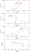 |
Fig. 14. Comparison of CNO elemental abundances of mixed and unmixed stars with HD 20 shown in blue for comparison. Gray circles resemble the study by Gratton et al. (2000) while red triangles indicate the stars published in Spite et al. (2005, 2006). Two C-rich stars were excluded from the latter sample. Lower limits on 12C/13C are indicated by upward pointing arrows and the classification into mixed and unmixed stars according to the authors are represented by open and filled symbols, respectively. The red line in the lower panel mimics the linear relation between [N/O] and [O/H] for mixed stars as reported by Spite et al. (2005), whereas the dashed line extrapolates the same relation to higher values of [O/H]. |
5.2. HD 20’s evolutionary state
Earlier works on HD 20 assumed it to be a red horizontal branch star (e.g., Gratton et al. 2000; Carney et al. 2003). Given our newly derived set of fundamental parameters, we can neither reject nor confirm this hypothesis. In Fig. 15, we illustrate HD 20’s position in the space of the structural parameters Teff, log L/L⊙, and log g together with an isochrone from the Dartmouth Stellar Evolution Database (Dotter et al. 2008). The model parameters were selected to resemble the findings in the present work, that is, an age of 11 Gyr (Sect. 5.6), [Fe/H] = −1.60 dex, as well as [α/Fe] = 0.40 dex (Sect. 5.3). The impacts from uncertainties in the two input parameters that affect the isochrone most – the stellar age and [Fe/H] – are indicated by representative error margins. While we adopted a standard scaling for the He mass fraction (Y = 0.245 + 1.5 ⋅ Z) for the latter model, we furthermore show the case of an extreme He enhancement of Y = 0.4. In addition, a set of He-burning tracks for three different stellar masses (0.70, 0.85, and 0.9 M⊙) from the Dartmouth database are depicted in the same plot.
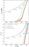 |
Fig. 15. Kiel diagram (upper panel) and Hertzsprung-Russell diagram (lower panel) with isochrones and helium burning tracks. HD 20’s position is depicted by a blue filled circle with error bars. Upper panel: the error on the gravity is smaller than the circle size. The red line represents a He-normal 11 Gyr isochrone at [Fe/H] = −1.60 dex, and [α/Fe] = +0.4 dex with age and metallicity error margins shown by orange and blue ranges. The RGB luminosity bump for this particular model at log L/L⊙ ∼ 2.0 is highlighted in the lower panel by an arrow and the label “LB”. The light blue curve is a model with the same parameters except for Y = 0.4. He-burning tracks for three different masses are shown by gray lines of different line styles with the stellar masses being indicated next to the respective tracks. |
Given its luminosity and gravity (log L/L⊙ = 1.78 and log g = 2.366), HD 20 appears too warm for a ∼11 Gyr old classical red giant, though the implied mass from the isochrone of 0.84 M⊙ resides within one standard deviation of our mass estimate (0.76 ± 0.08 M⊙). On the other hand, taking our asteroseismic mass and L for granted, HD 20 would be between 250 K and 350 K too cool to be consistent with the models for the horizontal branch, depending on whether a one-sigma or spot-on agreement is desired. This appears unfeasible even for slightly warmer photometric temperature scales (Appendix A.1.3). Still, the circumstance that sets our star as significantly fainter than the luminosity bump of the presented isochrone at log L/L⊙ ∼ 2.0 while nonetheless exhibiting mixing signatures (see the previous section) points towards a scenario where HD 20 has already evolved all the way through the red giant phase and is, in fact, now a horizontal branch star.
An alternative hypothesis for explaining HD 20’s position in the Hertzsprung-Russell diagram would be a non-standard He content as the model with strongly increased Y poses a considerably better fit to the observations. Such extreme levels of He have been found for second-generation stars in the most massive globular clusters (Milone et al. 2018; Zennaro et al. 2019). Nevertheless, characteristic chemical signatures of these peculiar stars are strong enhancements in light elements such as N, Na, and Al in lockstep with depletions of O and Mg (e.g., Bastian & Lardo 2018); none of which were found here (see Sects. 5.1 and 5.3). As a consequence, it is unlikely that HD 20 is a classical red giant star with high Y.
Unfortunately, our TESS light curve of HD 20 cannot be used to analyze the period spacing of the l = 1 mixed gravity and pressure modes to distinguish between helium-burning and non-helium-burning evolutionary stages as described by, for instance, Bedding et al. (2011) and Mosser et al. (2012a). To achieve this, a much longer time baseline than the available 27 days would be required in order to allow for a finer scanning of the frequencies around fmax and the identification of subordinate peaks in the power spectrum.
5.3. Abundances up to Zn (11 ≤ Z ≤ 30)
We could deduce abundances for 22 species of 17 chemical elements in the range 8 ≤ Z ≤ 30. For the α-elements Mg, Si, S, Ca, and Ti, we report a mean enhancement of [α/Fe] = 0.45 dex in LTE, which is in disagreement with the finding by Barklem et al. (2005), where a conversion to the Asplund et al. (2009) scale yields ![$ \frac{1}{3}[(\mathrm{Mg}\mathrm{+Ti}+\mathrm{Ca})/\mathrm{Fe}]\approx0.23 $](/articles/aa/full_html/2020/03/aa37189-19/aa37189-19-eq38.gif) dex. The discrepancy is alleviated when using the same elements for comparison, that is,
dex. The discrepancy is alleviated when using the same elements for comparison, that is, ![$ \frac{1}{3}[(\mathrm{Mg}+{\mathrm{Ti}\,\textsc{i}}+\mathrm{Ca})/\mathrm{Fe}]=0.34\pm0.13 $](/articles/aa/full_html/2020/03/aa37189-19/aa37189-19-eq39.gif) dex or
dex or ![$ \frac{1}{3}[(\mathrm{Mg}+{\mathrm{Ti}\,\textsc{ii}}+\mathrm{Ca})/\mathrm{Fe}]=0.38\pm0.07 $](/articles/aa/full_html/2020/03/aa37189-19/aa37189-19-eq40.gif) dex. In light of Appendix B.2, the origin for the observed difference is likely to be tied to their substantially hotter Teff (see discussion in Appendix A.1.3). Our value is typical for MW field stars at this [Fe/H] where nucleosynthetic processes in massive stars have played a dominant role in the enrichment of the ISM and supernovae of type Ia (mostly Fe-peak yields) have not yet started to contribute (e.g., McWilliam 1997). A minimum χ2 fit to the SN yields from Heger & Woosley (2010) using StarFit12 (see Placco et al. 2016; Chan & Heger 2017; Fraser et al. 2017, for detailed discussions) shows that the lighter elements of HD 20 – in NLTE – can be well reproduced by a ∼11.6 M⊙ faint CCSN with an explosion energy of 0.6 × 1051 erg. We stress that at HD 20’s metallicity we are likely not dealing with a single SN enrichment. Nevertheless, we are looking for a dominant contribution, which might survive even if it is highly integrated over time.
dex. In light of Appendix B.2, the origin for the observed difference is likely to be tied to their substantially hotter Teff (see discussion in Appendix A.1.3). Our value is typical for MW field stars at this [Fe/H] where nucleosynthetic processes in massive stars have played a dominant role in the enrichment of the ISM and supernovae of type Ia (mostly Fe-peak yields) have not yet started to contribute (e.g., McWilliam 1997). A minimum χ2 fit to the SN yields from Heger & Woosley (2010) using StarFit12 (see Placco et al. 2016; Chan & Heger 2017; Fraser et al. 2017, for detailed discussions) shows that the lighter elements of HD 20 – in NLTE – can be well reproduced by a ∼11.6 M⊙ faint CCSN with an explosion energy of 0.6 × 1051 erg. We stress that at HD 20’s metallicity we are likely not dealing with a single SN enrichment. Nevertheless, we are looking for a dominant contribution, which might survive even if it is highly integrated over time.
Overall, we find an excellent agreement of the deduced abundances with the field population at similar metallicities as demonstrated in Fig. 16, where our findings are overlayed on top of the sample of metal-poor stars by Roederer et al. (2014). For elements with two available species we only present one representative. There are only two departures from the general trends: O and Co, which both are enhanced in comparison. However, as already noted in Roederer et al. (2014), the reference sample shows trends with stellar parameters – most notably Teff – and thus evolutionary state. For elements heavier than N, mixing (Sect. 5.1) cannot be responsible for these trends, hence indicating contributions from systematic error sources in the abundance analyses. We therefore compare HD 20 to HD 222925, a star that was recently studied in great detail by Roederer et al. (2018b) and found to occupy a similar parameter space (Teff = 5636 K, log g = 2.54 dex, and [Fe/H] = −1.47 dex). Its light-element abundances are also indicated in Fig. 16 and we present a differential comparison in Fig. 17. After correcting for the difference in metallicity (0.13 dex), we find a remarkable match between the two stars in the considered range (reduced χ2 of 0.49). Similarities between the two stars have already been reported in the literature from a kinematical point of view (Roederer et al. 2018a) and based on their metallicity (Barklem et al. 2005; Roederer et al. 2018b). We emphasize, however, that the similarities do not extend to the neutron-capture regime, since HD 222925 is an r-II and HD 20 an r-I star with possible s-process contamination, as outlined in the following section.
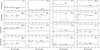 |
Fig. 16. Comparison of HD 20 (blue circle) to the metal-poor field star compilation (gray dots) by Roederer et al. (2014) and the red horizontal branch star HD 222925 (Roederer et al. 2018b, red circle). Dark blue circles and error bars indicate the result in LTE while the light blue circles indicate the NLTE-corrected ones. In the reference samples, corrections have been applied to O I, Na I, and K I. On the abscissa we show abundances from Fe II since these are less prone to departures from the LTE assumption (Sect. 3.3). |
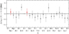 |
Fig. 17. Residual abundance pattern from O to Zn between HD 20 and HD 222925 after scaling by the difference in log ϵ(Fe II) of 0.13 dex. NLTE abundances were used for both stars for Na I and K I (red filled circles). |
5.4. Neutron-capture elements (Z > 30)
In order to delineate the nucleosynthetic processes that contributed to the observed abundances of heavy elements (Z > 30) in HD 20, we compare to a set of observed and predicted patterns. Following the classification scheme by Beers & Christlieb (2005), our findings of [Eu/Fe] = +0.73 dex and [Ba/Eu] = −0.38 dex place HD 20 in the regime of a typical r-I star. As indicated by the comparison in the top and middle panels of Fig. 18, HD 20’s heavy-element pattern from Nd to Ir (60 ≤ Z ≤ 77) is consistent with the scaled solar r-process by Sneden et al. (2008) when considering observational errors. In the light neutron-capture regime from Sr to Ag (38 ≤ Z ≤ 47), however, the agreement is poor. This behavior is archetypal for r-process rich stars (e.g., Roederer et al. 2018b) and led to the postulation of the existence of an additional, low-metallicity primary production channel of yet to be identified origin (the so-called weak r or lighter element primary process, McWilliam 1998; Travaglio et al. 2004; Hansen et al. 2012, 2014).
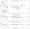 |
Fig. 18. Neutron-capture abundance pattern in LTE. Upper panel: HD 20’s heavy element abundances are indicated in blue. Shown in gray and red are abundances of the r-II star CS 22892−052 by Sneden et al. (2003) and the r-I star BD +17 3248 by Cowan et al. (2002) with updates from Cowan et al. (2005) and Roederer et al. (2010). The omitted Lu abundance for BD +17 3248 (see main text) is depicted in light red. Both patterns were scaled to achieve the overall best match to HD 20 in the entire considered range. The gray solid line denotes the solar-scaled r pattern from Sneden et al. (2008) and the best-fit AGB model (see text) is represented by dotted lines. Middle panel: residual pattern between HD 20 and the solar r pattern (gray line), CS 22892−052 (gray), and BD +17 3248 (red). Lower panel: residual pattern after mixing a contribution from BD +17 3248 with s-process material from the AGB yield model. |
In Fig. 18, we conduct a further comparison with the well-studied benchmark r-II and r-I stars CS 22892−052 (Sneden et al. 2003) and BD +17 3248 (Cowan et al. 2002, 2005; Roederer et al. 2010). The latter is a red horizontal branch star that is reasonably close to HD 20 in stellar parameter space (Teff = 5200 K, log g = 1.80 dex, [M/H] = −2.0 dex, vmic = 1.9 km s−1) – a circumstance that effectively reduces the impact of systematics (e.g., due to NLTE effects, see also Appendix B.2) on differential comparisons. In our analyses, we omitted the Lu abundance for BD +17 3248 from the UV Lu II line reported by Roederer et al. (2010), because – regardless of the substantial quoted error of 0.3 dex – it appears to represent a strong, likely unphysical outlier. We stress that neither of the abundance patterns attributed to the two stars is necessarily a tracer of a pure nuclear process. In contrast, they are likely to represent integrated signatures with different contributions from both the main and weak primary r-components (cf., Li et al. 2013; Hansen et al. 2014). The abundances in the range of 38 ≤ Z ≤ 90 for the two reference stars were scaled such that the reduced sum of the normalized quadratic deviations,  , was minimized (see middle panel of Fig. 18). Both patterns reproduce the depression of Y between Sr and Zr ([Y/⟨(Sr,Zr)⟩]= − 0.33 dex) and the deviation of Ag from the solar r-process. This points towards an enrichment contribution to HD 20 by the weak r-process as postulated earlier.
Nevertheless, the overall residual abundances from Sr to Zr as well as from Ba to Pr appear enhanced with respect to the heavy r-nuclei (Z ≥ 60). Another particularly outstanding residual feature is a statistically significant downward trend from Ba to Yb, which seems slightly less pronounced in the comparison involving BD +17 3248. In Solar system material, the lighter elements in question have dominant contributions from the s-process (Bisterzo et al. 2014; Prantzos et al. 2019), leading to the intriguing conclusion that, despite its moderately low metallicity, HD 20’s natal cloud might have been polluted with s-process material. In order to test this hypothesis, we mixed the pattern of BD +17 3248 as proxy for an integrated r-process pattern with main s-process yield models for thermally pulsing AGB stars with a standard 13C pocket from the FUll-Network Repository of Updated Isotopic Tables & Yields (F.R.U.I.T.Y. Cristallo et al. 2011). An upper metallicity limit was placed at [Fe/H] = −1.6 (Z = 0.0003), since it is infeasible for AGB polluters to have had higher [Fe/H] than HD 20 itself. We retrieved models for all remaining metallicities, stellar masses, and rotational velocities available through F.R.U.I.T.Y. In addition, a set of newly computed models with initial rotational speeds of 30 and 60 km s−1 for stellar masses of 2 and 5 M⊙ was included.
In the past, rotation has been considered as a potential process able to reproduce the observed spread in s-process elements at various metallicities (see Piersanti et al. 2013, and references therein). However, depending on the adopted physical prescriptions, different results have been obtained (see, e.g., Langer et al. 1999; Siess et al. 2004; den Hartogh et al. 2019). Moreover, it has to be taken into account that recent asteroseismic measurements of low-mass stars in the Galactic disk (see, e.g., Mosser et al. 2012b) demonstrated that stars belonging to the red clump region are characterized by slowly rotating cores. This latter feature tends to exclude the possibility to have fast-rotating cores for low-mass AGB stars in the solar neighborhood (which is an essential condition in order to have sizeable effects lead by rotation-induced mixing). However, the same has not yet been confirmed for stars with larger masses (M > 3 M⊙) and/or at low metallicities ([Fe/H] < −1 dex).
The optimal mixture of integrated r- and main s-contributions to the overall neutron-capture budget of HD 20 was obtained by minimizing the expression
with a and b being the weight coefficients for the two r and s template patterns and the index i denoting those individual elements in the range 38 ≤ Z ≤ 90 with available entries for the HD 20 pattern, the BD +17 3248 pattern, and the AGB yield tables.
A decisive observational quantity for pinpointing the AGB model mass is the ratio [hs/ls] of mean abundances for the heavy-s (hs, represented by Ba, La, and Ce) and light-s (ls, represented by Sr, Y, and Zr) elements. The models predict supersolar [hs/ls] at low masses (≲3 M⊙) with a decreasing trend with increasing model mass. Close-to Solar ratios are found in the region between 3 M⊙ and 5 M⊙. This behavior is demonstrated in Fig. 19, where we also indicate the Solar [hs/ls] measured for HD 20 (0.00 dex13). We conclude that main s-process contributions are likely to originate from high-mass (> 3 M⊙) AGB stars. This is bolstered by only being able to deduce an upper limit for HD 20’s Pb abundance – an element that is predicted to have strong contributions from models with masses < 5 M⊙ (e.g., Bisterzo et al. 2012; Cristallo et al. 2015). The large contribution to Pb comes from the radiative burning of the 13C(α,n)16O reaction (see Straniero et al. 1995), which is the dominant source in low-mass AGB stars. On the other hand, in more massive AGBs major neutron bursts come from the 22Ne(α,n)25Mg reaction, which is efficiently activated at the bottom of the convective shells during thermal pulses. These episodes commonly lead to minor Pb production14. At the same time, it is expected to find large Rb excesses from these massive AGB stars and their 22Ne(α,n)25Mg neutron source, manifesting in, for example, supersolar [Rb/Zr] (García-Hernández et al. 2009; Pérez-Mesa et al. 2017). For HD 20, we found [Rb/Zr] < 0.55 dex from the upper limit on the Rb abundance and after filtering our Zr finding from its dominant r-process contribution (see later in this section). This upper limit is ∼0.2 dex higher than the largest predictions from our employed, massive (i.e., 4−5 M⊙) AGB models. A robust measurement of Rb could be used to place further constraints on the exact initial mass of the polluting AGB star. In order to achieve this, spectra with an even higher S/N in the region around 7800 Å are required.
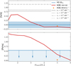 |
Fig. 19. Comparison of [hs/ls] and upper limit on [Pb/hs] for HD 20 against AGB s-process models of different initial masses. The value determined for HD 20 is indicated by blue horizontal lines and error margins, while models of Z = 0.0001 without rotation are shown in red. The adopted best-fit model with a rotation of 30 km s−1 is depicted in orange. For juxtaposition, we show i-process predictions for [hs/ls] from Hampel et al. (2016) for four different neutron densities, ni, in the upper panel using black dotted, dash-dotted, dashed, and solid lines (see legend). |
By minimizing Eq. (9), we found the best-fit ( ) AGB model to be the one with 5 M⊙, Z = 0.0001 ([Fe/H] ≈ −2.15 dex) and a rotational velocity of 30 km s−1. Here the model with non-zero angular momentum poses a slightly better fit than its non-rotating counterpart with all other parameters kept fixed (see also Fig. 19 top panel). The adopted mixture can successfully reproduce the entire neutron-capture pattern in HD 20. This includes the observations for the commonly employed tracers [hs/ls] and [Ba/Eu], as well as the downward trend from Ba to Yb that persists when assuming an r-only enrichment.
Using yields from the aforementioned main s-model and the BD +17 3248 pattern together with the best-fit model parameters for Eq. (9), we can estimate the fractional (integrated) r- and (main) s-process contributions to individual elements in HD 20 through
In order to properly account for fit uncertainties, we sampled the posterior distribution of the parameters a and b with emcee using the abundance errors. In Fig. 20 we show 800 individual realizations of the samples. From these, the fractions and asymmetric limits were estimated from the median, the 15.9th, and the 84.1th percentiles, respectively. These are listed in Table 5.
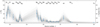 |
Fig. 20. Estimated r- (right-hand scale) and s-fractions (left-hand scale) in HD 20 based on Eq. (10) with BD +17 3248 as proxy for an r pattern and the best-fit AGB model representing the s-enrichment site. Shown are only those elements that have a measured abundance in BD +17 3248. |
Estimated fractional contributions from the r- and s-process for elements with Z ≥ 38 in HD 20.
We find significant s-process fractions above 30% for the elements Sr, Y, Zr, and Ba, whereas only Y might have had a dominant (fs > 50%) enrichment contribution from the s-process. This could be corroborated by measuring isotopic fractions for selected elements from spectra at very high resolution (e.g., Mashonkina & Belyaev 2019), though we note that HD 20 shows considerable intrinsic line broadening signatures (Sect. 3.5) that may exceed the hyperfine splitting effect.
An important question that should be answered with respect to our proposed s-process imprint is whether the finding is caused by mixing in the ISM prior to the formation of HD 20 or whether it is a result of surface pollution via mass transfer in a binary system (e.g., Gull et al. 2018). The latter option was ruled out with high confidence in Sect. 2.2, where we showed a lack of radial velocity variation. Therefore, a binary signal could only be hidden if the orbit would be seen almost perfectly face-on. Consequently, we strongly prefer the scenario where HD 20 had its chemical pattern composition mixed in the ISM.
5.5. i-process considerations
Another metal-poor star with signatures of simultaneous overabundances in both s- and r-process material is HD 94028. Among others, this star has been studied spectroscopically by Roederer (2012) and Roederer et al. (2016), who complemented the abundance pattern from elements typically found in the optical with more exotic species (e.g., Ge, As, Se) that are only measurable in ultraviolet spectra gathered with the Hubble Space Telescope (HST). The authors concluded that several abundance ratios – most notably supersolar [As/Ge], [Mo/Fe], and [Ru/Fe] – are poorly described by combinations of s- and r-process patterns and therefore suggested an additional contribution by the i-process. However, more recently, Han et al. (2018) indicated that both [As/Ge] and [Mo/Ru] may be well explained by weak r-nucleosynthesis without the need for an additional i-process. The i-process was also proposed by Koch et al. (2019) as a candidate to reproduce their observed pattern for a metal-poor bulge star (labeled #10464, following the naming convention in Koch et al. 2016). The authors find that either a mixture of an i-pattern with a main s-pattern or an i-process with two proton ingestion events reproduces their observations best.
Based on Fig. 19, the residual [hs/ls] of HD 20 is seen to be well described by a 5 M⊙ rotating AGB star, while the i-process of intermediate neutron densities predicts much too high [hs/ls] ratios. In any case, we compare HD 20 to the two supposedly i-enriched stars to search for i-process indications in the patterns. By comparing to the filtered patterns of HD 94028–(r + s) and #10464–s (Fig. 21), no clear i-process features stand out, and we cannot claim any i-process contribution in HD 20. However, some weak r-enrichment might have taken place. Until further i-process indications, such as elemental ratios [As/Ge] or strong pattern trends can robustly be associated with the i-process, it is hard to observationally investigate such contaminations. In order to test [As/Ge] we would need HST data.
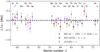 |
Fig. 21. Comparison of the residual HD 20 pattern (purple, same as lower panel of Fig. 18) to the patterns of HD 94028 (red) and #10464 (green) after subtracting r + s and s contributions, respectively. The residual pattern for HD 94028 was determined following the procedure outlined in Sect. 5.2 in Roederer et al. (2016), whereas a Z = 0.0001, 2 M⊙ AGB model was assumed for the s-enrichment in #10464. |
5.6. Cosmochronological age
Measuring a reliable abundance for the radioactive element Th enables an estimation of HD 20’s age from nuclear cosmochronology. The only isotope of Th with a lifetime that is relevant on cosmological timescales is 232Th (τ1/2 = 14.05 Gyr). The currently observed ratio log ϵ(Th/r) of Th and other, stable r-elements can be related to a decay time using a theoretical initial production ratio, log ϵ(Th/r)0, together with the age relation,

as outlined by Cayrel et al. (2001). For Table 6, we considered the reference elements Eu and Hf as well as the third-peak elements Os and Ir. Moreover, we obtained a lower-limit age of 7.8 Gyr from our upper limit on the U abundance. Despite considerable ambiguities in theoretical production ratios (e.g., Schatz et al. 2002; Cowan et al. 1999), the dominant source of error for the inferred ages is the combined uncertainty of the abundances for each pair, which amounts to  dex. The latter uncertainty is linearly propagated into an age error of 6.5 Gyr (see also Ludwig et al. 2010, for a detailed discussion of other error sources). According to Cayrel et al. (2001), the observational and theoretical uncertainties are minimized by using Os and Ir as baseline for the chronometers, since they are closest to Th in atomic number. However, we note that both Os and Ir were determined from the neutral species while our Th abundance was deduced from the singly ionized state, which potentially introduces biases due to NLTE effects15. As indicated by Hansen et al. (2018b), NLTE effects on Th II abundances may be alleviated by introducing a full, 3D NLTE treatment. Hence the obtained abundance would be close to our 1D LTE estimate.
Age estimates from different radioactive chronometers.
The age of 26.0 Gyr from Th/Hf appears unreasonably high and we note that Roederer et al. (2009) reported a similar behavior for this chronometer. We thus suspect that the initial production rates are overestimated, which might be connected to a breakdown of the robustness of the heavy r-pattern in the region around Hf (M. Eichler, priv. comm.). Removing our estimated high s-process contribution (19.4%) for Hf only decreases the deduced age slightly, by about 4 Gyr. In any case, we exclude the corresponding age from consideration and calculate a mean age of 11.0 ± 3.8 Gyr from the remaining three actual detections (10.0, 11.3, and 11.6 Gyr, thereby excluding the lower limit involving U).
6. Summary and conclusions
We present a detailed investigation of the chemical composition of the metal-poor ([Fe/H] = −1.60 dex), r-process enhanced (r-I) Galactic halo star HD 20. Using newly obtained and archival very high S/N and high-resolution spectra in concert with extensive photometry and astrometry from the Gaia and TESS missions, we carefully investigate the key fundamental stellar parameters, which are independently confirmed by a number of alternative approaches. These allow for a high-precision spectroscopic chemical analysis, yielding abundances for 25 species of 20 elements with Z ≤ 30, as well as for 29 species of 28 neutron-capture elements. Hence, we report on abundances for in total 48 elements, thereby adding 26 elements to the largest existing study of this star by Barklem et al. (2005). Moreover, we deduce meaningful upper limits for Li, Rb, Pb, and U. This renders our presented abundance pattern one of the most complete available to date and therefore adds HD 20 to the short list of benchmark stars for nuclear astrophysics involving traces of only r + s processes.
Regarding the light elements up to Zn, we find a behavior typical for the Galactic halo at comparable metallicities indicative of an enrichment history dominated by CCSNe prior to the onset of contributions by supernovae of type Ia. Using yield models, we could show that faint CCSNe of progenitor masses around ∼11.6 M⊙ and explosion energies ∼0.6 × 1051 erg can explain the light-element pattern in HD 20. While the heavy neutron-capture elements are found to closely follow the solar r-process distribution, strong deviations are found with respect to the first-peak elements, primarily due to depletions in Y and Ag. We attribute this observation to the additional primary (weak) r-process acting at low metallicity that was postulated based on observations of other metal-poor stars (e.g., Hansen et al. 2012). This emphasizes that the Solar-scaled r-pattern cannot pose as a universal proxy for the r-process, particularly in the lighter neutron-capture regime.
In comparing our observed neutron-capture abundances to the benchmark r-I star BD +17 3248 – which was chosen in order to lessen the gravity of systematic abundance errors – we find that several elements (Sr, Y, Zr, Ba, La) that are commonly associated with the s-process appear to be enhanced in HD 20 with respect to a pure r-process pattern. We obtain a considerably better fit of the overall distribution by introducing a dilution with material from main s-process yield predictions of a low-metallicity, massive, and rotating AGB star. Based on this model, we estimate a dominant s-process fraction for Y ( %), whereas several other elements may still have a significant contribution from this production channel (Table 5, Fig. 20). Given the abundance pattern for HD 20 presented here, we prefer an r + s mixing scenario and refute i-process contributions until more robust abundance ratios or patterns will be proposed. Based on the lack of evidence of HD 20 being part of a binary system, we propose that the mixing happened in the ISM prior to the star’s formation as opposed to surface pollution due to mass transfer from a companion.
HD 20’s age is estimated at 11.0 ± 3.8 Gyr based on nuclear cosmochronology from abundance ratios involving the radioactive element Th. We caution, however, that there are statistical and systematic error sources of both observational and theoretical nature that may bias this measure. Nonetheless, it appears safe to assume that the star is a representative of the old Galactic halo.
A future perspective for work on HD 20 is to complement our abundance pattern with UV spectra from HST. Deriving abundances from UV lines is extremely important in order to obtain more complete patterns. Key elements like As and Au carry important information on the neutron-capture environment and can only be assessed in HST data. Arsenic could contain crucial clues on the i-process, which we cannot explore in the ground-based, spectroscopically derived abundances, and Au is a good r-process indicator. An additional element that is more easily measured in the UV is Pb, which is an important s-process tracer for which we could only deduce an upper limit abundance in this study. Furthermore, understanding how and if the neutron-capture processes are formed and incorporated into later generations of stars is crucial to understand the need for an i-process versus efficient and fast mixing of r + s-process material in the ISM. Here HD 20 offers promising insights into the neutron-capture processes as it is slightly enhanced and we detect clear traces of both r and s. It poses a powerful benchmark and it is far less polluted than the Sun.
Section 5.3.7 of the Gaia Data Release 2 Documentation release 1.2: https://gea.esac.esa.int/archive/documentation/GDR2/
https://github.com/alexji/moog17scat as of November 2018.
Bergemann et al. (2012b) mention a Sr II line at 4167.8 Å in their Table 1. However the line parameters provided are for the line at 4161.8 Å. NLTE corrections are not provided for this transition.
Furthermore, as demonstrated in Appendix B.2, among all relevant elements the two referred ones are most sensitive to uncertainties in the model temperature.
We emphasize that this step is not utterly important at this point, because the ATHOS implementation for Teff is largely insensitive to rotational broadening (see Hanke et al. 2018). Line broadening, however, does affect ATHOS’ [Fe/H] estimators (Appendix A.2).
Acknowledgments
M.H., H.-G.L., and E.K.G. gratefully acknowledge support by the Deutsche Forschungsgemeinschaft (DFG, German Research Foundation) – Project-ID 138713538 – SFB 881 (“The Milky Way System”, subprojects A03, A04, and A08). C.J.H. acknowledges support from the Max Planck Society and the “ChETEC” COST Action (CA16117), supported by COST (European Cooperation in Science and Technology). The authors are grateful to M. Catelan, A. Koch, Z. Prudil, and A. Gallagher for fruitful discussions. Furthermore, the help by M. Kovalev and M. Bergemann in setting up a grid of NLTE corrections for Fe lines is highly appreciated. A. Heger and C. Chan are acknowledged for their detailed support for the application of StarFit. We thank T. Nordlander and K. Lind for providing access to their grid of NLTE corrections for Al. We value the swift and constructive report issued by the anonymous referee. This work has made use of the VALD database, operated at Uppsala University, the Institute of Astronomy RAS in Moscow, and the University of Vienna. This paper presents results from the European Space Agency (ESA) space mission Gaia. Gaia data are being processed by the Gaia Data Processing and Analysis Consortium (DPAC). Funding for the DPAC is provided by national institutions, in particular the institutions participating in the Gaia MultiLateral Agreement (MLA). The Gaia mission website is https://www.cosmos.esa.int/gaia. This paper includes data collected by the TESS mission. Funding for the TESS mission is provided by the NASA Explorer Program. This research made use of Lightkurve, a Python package for Kepler and TESS data analysis (Lightkurve Collaboration 2018).
References
- Abbott, B. P., Abbott, R., Abbott, T. D., et al. 2017, Phys. Rev. Lett., 119, 161101 [NASA ADS] [CrossRef] [PubMed] [Google Scholar]
- Alonso, A., Arribas, S., & Martinez-Roger, C. 1994, A&AS, 107, 365 [NASA ADS] [Google Scholar]
- Alonso, A., Arribas, S., & Martínez-Roger, C. 1999a, A&AS, 140, 261 [NASA ADS] [CrossRef] [EDP Sciences] [Google Scholar]
- Alonso, A., Arribas, S., & Martínez-Roger, C. 1999b, A&AS, 139, 335 [NASA ADS] [CrossRef] [EDP Sciences] [Google Scholar]
- Alonso, A., Arribas, S., & Martínez-Roger, C. 2001, A&A, 376, 1039 [NASA ADS] [CrossRef] [EDP Sciences] [Google Scholar]
- Amarsi, A. M., Nordlander, T., Barklem, P. S., et al. 2018, A&A, 615, A139 [NASA ADS] [CrossRef] [EDP Sciences] [Google Scholar]
- Amarsi, A. M., Nissen, P. E., & Skúladóttir, Á. 2019, A&A, 630, A104 [NASA ADS] [CrossRef] [EDP Sciences] [Google Scholar]
- Andrae, R., Fouesneau, M., Creevey, O., et al. 2018, A&A, 616, A8 [NASA ADS] [CrossRef] [EDP Sciences] [Google Scholar]
- Andrievsky, S. M., Spite, F., Korotin, S. A., et al. 2011, A&A, 530, A105 [NASA ADS] [CrossRef] [EDP Sciences] [Google Scholar]
- Anthony-Twarog, B. J., & Twarog, B. A. 1994, AJ, 107, 1577 [NASA ADS] [CrossRef] [Google Scholar]
- Arcones, A., Janka, H. T., & Scheck, L. 2007, A&A, 467, 1227 [NASA ADS] [CrossRef] [EDP Sciences] [Google Scholar]
- Asplund, M., Grevesse, N., Sauval, A. J., & Scott, P. 2009, ARA&A, 47, 481 [NASA ADS] [CrossRef] [Google Scholar]
- Bailer-Jones, C. A. L., Rybizki, J., Fouesneau, M., Mantelet, G., & Andrae, R. 2018, AJ, 156, 58 [NASA ADS] [CrossRef] [Google Scholar]
- Bard, A., & Kock, M. 1994, A&A, 282, 1014 [NASA ADS] [Google Scholar]
- Bard, A., Kock, A., & Kock, M. 1991, A&A, 248, 315 [NASA ADS] [Google Scholar]
- Barklem, P. S., Stempels, H. C., Allende Prieto, C., et al. 2002, A&A, 385, 951 [NASA ADS] [CrossRef] [EDP Sciences] [Google Scholar]
- Barklem, P. S., Christlieb, N., Beers, T. C., et al. 2005, A&A, 439, 129 [NASA ADS] [CrossRef] [EDP Sciences] [Google Scholar]
- Bastian, N., & Lardo, C. 2018, ARA&A, 56, 83 [NASA ADS] [CrossRef] [Google Scholar]
- Battaglia, G., Irwin, M., Tolstoy, E., et al. 2008, MNRAS, 383, 183 [NASA ADS] [CrossRef] [MathSciNet] [Google Scholar]
- Bedding, T. R., Mosser, B., Huber, D., et al. 2011, Nature, 471, 608 [NASA ADS] [CrossRef] [PubMed] [Google Scholar]
- Beers, T. C., & Christlieb, N. 2005, ARA&A, 43, 531 [NASA ADS] [CrossRef] [Google Scholar]
- Beers, T. C., Flynn, C., Rossi, S., et al. 2007, ApJS, 168, 128 [NASA ADS] [CrossRef] [Google Scholar]
- Bergemann, M. 2011, MNRAS, 413, 2184 [NASA ADS] [CrossRef] [Google Scholar]
- Bergemann, M., & Gehren, T. 2008, A&A, 492, 823 [NASA ADS] [CrossRef] [EDP Sciences] [Google Scholar]
- Bergemann, M., Pickering, J. C., & Gehren, T. 2010, MNRAS, 401, 1334 [NASA ADS] [CrossRef] [Google Scholar]
- Bergemann, M., Lind, K., Collet, R., Magic, Z., & Asplund, M. 2012a, MNRAS, 427, 27 [NASA ADS] [CrossRef] [Google Scholar]
- Bergemann, M., Hansen, C. J., Bautista, M., & Ruchti, G. 2012b, A&A, 546, A90 [NASA ADS] [CrossRef] [EDP Sciences] [Google Scholar]
- Bergemann, M., Kudritzki, R.-P., Würl, M., et al. 2013, ApJ, 764, 115 [NASA ADS] [CrossRef] [Google Scholar]
- Bergemann, M., Serenelli, A., Schönrich, R., et al. 2016, A&A, 594, A120 [NASA ADS] [CrossRef] [EDP Sciences] [Google Scholar]
- Bergemann, M., Collet, R., Amarsi, A. M., et al. 2017a, ApJ, 847, 15 [NASA ADS] [CrossRef] [Google Scholar]
- Bergemann, M., Collet, R., Schönrich, R., et al. 2017b, ApJ, 847, 16 [NASA ADS] [CrossRef] [Google Scholar]
- Bergemann, M., Gallagher, A. J., Eitner, P., et al. 2019, A&A, 631, A80 [NASA ADS] [CrossRef] [EDP Sciences] [Google Scholar]
- Bernstein, R., Shectman, S. A., Gunnels, S. M., Mochnacki, S., & Athey, A. E. 2003, in Society of Photo-Optical Instrumentation Engineers (SPIE) Conference Series, eds. M. Iye, & A. F. M. Moorwood, Proc. SPIE, 4841, 1694 [NASA ADS] [Google Scholar]
- Bessell, M. S. 1983, PASP, 95, 480 [NASA ADS] [CrossRef] [Google Scholar]
- Biemont, E., Grevesse, N., Kwiatkovski, M., & Zimmermann, P. 1984, A&A, 131, 364 [NASA ADS] [Google Scholar]
- Biemont, E., Quinet, P., & Zeippen, C. J. 1993, A&AS, 102, 435 [NASA ADS] [Google Scholar]
- Biémont, E., Garnir, H. P., Palmeri, P., Li, Z. S., & Svanberg, S. 2000, MNRAS, 312, 116 [NASA ADS] [CrossRef] [Google Scholar]
- Bisterzo, S., Gallino, R., Straniero, O., Cristallo, S., & Käppeler, F. 2012, MNRAS, 422, 849 [NASA ADS] [CrossRef] [Google Scholar]
- Bisterzo, S., Travaglio, C., Gallino, R., Wiescher, M., & Käppeler, F. 2014, ApJ, 787, 10 [NASA ADS] [CrossRef] [Google Scholar]
- Bizzarri, A., Huber, M. C. E., Noels, A., et al. 1993, A&A, 273, 707 [NASA ADS] [Google Scholar]
- Blackwell, D. E., & Shallis, M. J. 1977, MNRAS, 180, 177 [NASA ADS] [CrossRef] [Google Scholar]
- Burbidge, E. M., Burbidge, G. R., Fowler, W. A., & Hoyle, F. 1957, Rev. Mod. Phys., 29, 547 [NASA ADS] [CrossRef] [Google Scholar]
- Burris, D. L., Pilachowski, C. A., Armandroff, T. E., et al. 2000, ApJ, 544, 302 [NASA ADS] [CrossRef] [Google Scholar]
- Busso, M., Gallino, R., Lambert, D. L., Travaglio, C., & Smith, V. V. 2001, ApJ, 557, 802 [NASA ADS] [CrossRef] [Google Scholar]
- Cameron, A. G. W. 1957, PASP, 69, 201 [NASA ADS] [CrossRef] [Google Scholar]
- Cameron, A. G. W. 2003, ApJ, 587, 327 [NASA ADS] [CrossRef] [Google Scholar]
- Campante, T. L., Corsaro, E., Lund, M. N., et al. 2019, ApJ, 885, 31 [NASA ADS] [CrossRef] [Google Scholar]
- Carney, B. W., Latham, D. W., Stefanik, R. P., Laird, J. B., & Morse, J. A. 2003, AJ, 125, 293 [NASA ADS] [CrossRef] [Google Scholar]
- Carney, B. W., Gray, D. F., Yong, D., et al. 2008, AJ, 135, 892 [NASA ADS] [CrossRef] [Google Scholar]
- Castelli, F., & Kurucz, R. L. 2003, in Modelling of Stellar Atmospheres, eds. N. Piskunov, W. W. Weiss, & D. F. Gray, IAU Symp., 210, A20 [Google Scholar]
- Cayrel, R., Hill, V., Beers, T. C., et al. 2001, Nature, 409, 691 [NASA ADS] [CrossRef] [PubMed] [Google Scholar]
- Chan, C., & Heger, A. 2017, 14th International Symposium on Nuclei in the Cosmos (NIC2016), 020209 [Google Scholar]
- Chornock, R., Berger, E., Kasen, D., et al. 2017, ApJ, 848, L19 [NASA ADS] [CrossRef] [Google Scholar]
- Corliss, C. H., & Bozman, W. R. 1962, Experimental Transition Probabilities for Spectral Lines of Seventy Elements; Derived from the NBS Tables of Spectral-line Intensities (Washington: US Department of Commerce) [CrossRef] [Google Scholar]
- Corsaro, E., & De Ridder, J. 2014, A&A, 571, A71 [NASA ADS] [CrossRef] [EDP Sciences] [Google Scholar]
- Corsaro, E., Mathur, S., García, R. A., et al. 2017, A&A, 605, A3 [NASA ADS] [CrossRef] [EDP Sciences] [Google Scholar]
- Côté, B., Eichler, M., Arcones, A., et al. 2019, ApJ, 875, 106 [NASA ADS] [CrossRef] [Google Scholar]
- Cowan, J. J., Pfeiffer, B., Kratz, K. L., et al. 1999, ApJ, 521, 194 [NASA ADS] [CrossRef] [Google Scholar]
- Cowan, J. J., Sneden, C., Burles, S., et al. 2002, ApJ, 572, 861 [NASA ADS] [CrossRef] [Google Scholar]
- Cowan, J. J., Sneden, C., Beers, T. C., et al. 2005, ApJ, 627, 238 [NASA ADS] [CrossRef] [Google Scholar]
- Cowley, C. R., & Corliss, C. H. 1983, MNRAS, 203, 651 [NASA ADS] [CrossRef] [Google Scholar]
- Creevey, O., Grundahl, F., Thévenin, F., et al. 2019, A&A, 625, A33 [NASA ADS] [CrossRef] [EDP Sciences] [Google Scholar]
- Cristallo, S., Piersanti, L., Straniero, O., et al. 2011, ApJS, 197, 17 [NASA ADS] [CrossRef] [Google Scholar]
- Cristallo, S., Straniero, O., Piersanti, L., & Gobrecht, D. 2015, ApJS, 219, 40 [NASA ADS] [CrossRef] [Google Scholar]
- Dekker, H., D’Odorico, S., Kaufer, A., Delabre, B., & Kotzlowski, H. 2000, in Optical and IR Telescope Instrumentation and Detectors, eds. M. Iye, & A. F. Moorwood, Proc. SPIE, 4008, 534 [Google Scholar]
- Den Hartog, E. A., Lawler, J. E., Sneden, C., & Cowan, J. J. 2003, ApJS, 148, 543 [Google Scholar]
- Den Hartog, E. A., Lawler, J. E., Sneden, C., & Cowan, J. J. 2006, ApJS, 167, 292 [NASA ADS] [CrossRef] [Google Scholar]
- Den Hartog, E. A., Lawler, J. E., Sobeck, J. S., Sneden, C., & Cowan, J. J. 2011, ApJS, 194, 35 [NASA ADS] [CrossRef] [Google Scholar]
- den Hartogh, J. W., Hirschi, R., Lugaro, M., et al. 2019, A&A, 629, A123 [NASA ADS] [CrossRef] [EDP Sciences] [Google Scholar]
- Dotter, A., Chaboyer, B., Jevremović, D., et al. 2008, ApJS, 178, 89 [NASA ADS] [CrossRef] [Google Scholar]
- Ducati, J. R. 2002, VizieR Online Data Catalog: II/237 [Google Scholar]
- ESA 1997, in The HIPPARCOS and TYCHO catalogues. Astrometric and photometric star catalogues derived from the ESA HIPPARCOS Space Astrometry Mission (Noordwijk, Netherlands: ESA Publications Division), ESA Spec. Publ., 1200 [Google Scholar]
- Foreman-Mackey, D., Hogg, D. W., Lang, D., & Goodman, J. 2013, PASP, 125, 306 [CrossRef] [Google Scholar]
- Fraser, M., Casey, A. R., Gilmore, G., Heger, A., & Chan, C. 2017, MNRAS, 468, 418 [NASA ADS] [CrossRef] [Google Scholar]
- Freytag, B., Steffen, M., Ludwig, H. G., et al. 2012, J. Comput. Phys., 231, 919 [Google Scholar]
- Fuhr, J. R., Martin, G. A., & Wiese, W. L. 1988, J. Phys. Chem. Ref. Data, 17, 504 [Google Scholar]
- Fulbright, J. P., & Johnson, J. A. 2003, ApJ, 595, 1154 [NASA ADS] [CrossRef] [Google Scholar]
- Gaia Collaboration (Brown, A. G. A., et al.) 2018, A&A, 616, A1 [NASA ADS] [CrossRef] [EDP Sciences] [Google Scholar]
- Gallino, R., Arlandini, C., Busso, M., et al. 1998, ApJ, 497, 388 [NASA ADS] [CrossRef] [PubMed] [Google Scholar]
- García-Hernández, D. A., Manchado, A., Lambert, D. L., et al. 2009, ApJ, 705, L31 [NASA ADS] [CrossRef] [Google Scholar]
- Garz, T. 1973, A&A, 26, 471 [NASA ADS] [Google Scholar]
- González Hernández, J. I., & Bonifacio, P. 2009, A&A, 497, 497 [NASA ADS] [CrossRef] [EDP Sciences] [Google Scholar]
- Gratton, R. G., Sneden, C., Carretta, E., & Bragaglia, A. 2000, A&A, 354, 169 [NASA ADS] [Google Scholar]
- Gull, M., Frebel, A., Cain, M. G., et al. 2018, ApJ, 862, 174 [NASA ADS] [CrossRef] [Google Scholar]
- Hampel, M., Stancliffe, R. J., Lugaro, M., & Meyer, B. S. 2016, ApJ, 831, 171 [NASA ADS] [CrossRef] [Google Scholar]
- Hampel, M., Karakas, A. I., Stancliffe, R. J., Meyer, B. S., & Lugaro, M. 2019, ApJ, 887, 11 [NASA ADS] [CrossRef] [Google Scholar]
- Han, W., Zhang, L., Yang, G., Niu, P., & Zhang, B. 2018, ApJ, 856, 58 [NASA ADS] [CrossRef] [Google Scholar]
- Hanke, M., Koch, A., Hansen, C. J., & McWilliam, A. 2017, A&A, 599, A97 [NASA ADS] [CrossRef] [EDP Sciences] [Google Scholar]
- Hanke, M., Hansen, C. J., Koch, A., & Grebel, E. K. 2018, A&A, 619, A134 [NASA ADS] [CrossRef] [EDP Sciences] [Google Scholar]
- Hannaford, P., Lowe, R. M., Grevesse, N., Biemont, E., & Whaling, W. 1982, ApJ, 261, 736 [NASA ADS] [CrossRef] [Google Scholar]
- Hansen, C. J., Primas, F., Hartman, H., et al. 2012, A&A, 545, A31 [NASA ADS] [CrossRef] [EDP Sciences] [Google Scholar]
- Hansen, C. J., Bergemann, M., Cescutti, G., et al. 2013, A&A, 551, A57 [NASA ADS] [CrossRef] [EDP Sciences] [Google Scholar]
- Hansen, C. J., Montes, F., & Arcones, A. 2014, ApJ, 797, 123 [NASA ADS] [CrossRef] [Google Scholar]
- Hansen, T. T., Andersen, J., Nordström, B., et al. 2015, A&A, 583, A49 [NASA ADS] [CrossRef] [EDP Sciences] [Google Scholar]
- Hansen, T. T., Holmbeck, E. M., Beers, T. C., et al. 2018a, ApJ, 858, 92 [NASA ADS] [CrossRef] [Google Scholar]
- Hansen, C. J., El-Souri, M., Monaco, L., et al. 2018b, ApJ, 855, 83 [NASA ADS] [CrossRef] [Google Scholar]
- Hauck, B., & Mermilliod, M. 1998, A&AS, 129, 431 [NASA ADS] [CrossRef] [EDP Sciences] [Google Scholar]
- Hawkins, K., Jofré, P., Heiter, U., et al. 2016, A&A, 592, A70 [NASA ADS] [CrossRef] [EDP Sciences] [Google Scholar]
- Heger, A., & Woosley, S. E. 2010, ApJ, 724, 341 [NASA ADS] [CrossRef] [Google Scholar]
- Heiter, U., Jofré, P., Gustafsson, B., et al. 2015, A&A, 582, A49 [NASA ADS] [CrossRef] [EDP Sciences] [PubMed] [Google Scholar]
- Hobbs, L. M., Thorburn, J. A., & Rebull, L. M. 1999, ApJ, 523, 797 [NASA ADS] [CrossRef] [Google Scholar]
- Høg, E., Fabricius, C., Makarov, V. V., et al. 2000, A&A, 355, L27 [Google Scholar]
- Ivarsson, S., Andersen, J., Nordström, B., et al. 2003, A&A, 409, 1141 [NASA ADS] [CrossRef] [EDP Sciences] [Google Scholar]
- Jayasinghe, T., Stanek, K. Z., Kochanek, C. S., et al. 2019, MNRAS, 485, 961 [NASA ADS] [CrossRef] [Google Scholar]
- Ji, A. P., Drout, M. R., & Hansen, T. T. 2019, ApJ, 882, 40 [NASA ADS] [CrossRef] [Google Scholar]
- Jofré, P., Heiter, U., Soubiran, C., et al. 2014, A&A, 564, A133 [NASA ADS] [CrossRef] [EDP Sciences] [Google Scholar]
- Jones, A., Noll, S., Kausch, W., Szyszka, C., & Kimeswenger, S. 2013, A&A, 560, A91 [NASA ADS] [CrossRef] [EDP Sciences] [Google Scholar]
- Karakas, A. I., & Lattanzio, J. C. 2014, PASA, 31, e030 [NASA ADS] [CrossRef] [Google Scholar]
- Kelson, D. D. 2003, PASP, 115, 688 [NASA ADS] [CrossRef] [Google Scholar]
- Kjeldsen, H., & Bedding, T. R. 1995, A&A, 293, 87 [NASA ADS] [Google Scholar]
- Kobayashi, C., Leung, S. C., & Nomoto, K. 2019, ApJ, submitted [arXiv:1906.09980] [Google Scholar]
- Koch, A., McWilliam, A., Preston, G. W., & Thompson, I. B. 2016, A&A, 587, A124 [Google Scholar]
- Koch, A., Reichert, M., Hansen, C. J., et al. 2019, A&A, 622, A159 [NASA ADS] [CrossRef] [EDP Sciences] [Google Scholar]
- Korotin, S. A. 2008, Odessa Astron. Publ., 21, 42 [NASA ADS] [Google Scholar]
- Korotin, S. A. 2009, Astron. Rep., 53, 651 [NASA ADS] [CrossRef] [Google Scholar]
- Korotin, S., Andrievsky, S., Caffau, E., & Bonifacio, P. 2017, in Stars: From Collapse to Collapse, eds. Y. Y. Balega, D. O. Kudryavtsev, I. I. Romanyuk, & I. A. Yakunin, ASP Conf. Ser., 510, 141 [Google Scholar]
- Korotin, S. A., Andrievsky, S. M., & Zhukova, A. V. 2018, MNRAS, 480, 965 [NASA ADS] [CrossRef] [Google Scholar]
- Kramida, A., Ralchenko, Yu., Reader, J., & NIST ASD Team 2018, NIST Atomic Spectra Database (ver. 5.6.1), [Online]. Available: https://physics.nist.gov/asd [2019, August 19] National Institute of Standards and Technology, Gaithersburg, MD [Google Scholar]
- Kratz, K.-L., Farouqi, K., Pfeiffer, B., et al. 2007, ApJ, 662, 39 [NASA ADS] [CrossRef] [MathSciNet] [Google Scholar]
- Kurucz, R. L., & Bell, B. 1995, Atomic Line List (Cambridge, MA: Smithsonian Astrophysical Observatory) [Google Scholar]
- Kwiatkowski, M., Zimmermann, P., Biemont, E., & Grevesse, N. 1982, A&A, 112, 337 [NASA ADS] [Google Scholar]
- Langer, N., Heger, A., Wellstein, S., & Herwig, F. 1999, A&A, 346, L37 [Google Scholar]
- Lattimer, J. M., & Schramm, D. N. 1974, ApJ, 192, L145 [Google Scholar]
- Lawler, J. E., & Dakin, J. T. 1989, J. Opt. Soc. Am. B Opt. Phys., 6, 1457 [NASA ADS] [CrossRef] [Google Scholar]
- Lawler, J. E., Bonvallet, G., & Sneden, C. 2001a, ApJ, 556, 452 [NASA ADS] [CrossRef] [Google Scholar]
- Lawler, J. E., Wickliffe, M. E., den Hartog, E. A., & Sneden, C. 2001b, ApJ, 563, 1075 [CrossRef] [Google Scholar]
- Lawler, J. E., Wyart, J.-F., & Blaise, J. 2001c, ApJS, 137, 351 [NASA ADS] [CrossRef] [Google Scholar]
- Lawler, J. E., Wickliffe, M. E., Cowley, C. R., & Sneden, C. 2001d, ApJS, 137, 341 [NASA ADS] [CrossRef] [Google Scholar]
- Lawler, J. E., Sneden, C., & Cowan, J. J. 2004, ApJ, 604, 850 [NASA ADS] [CrossRef] [Google Scholar]
- Lawler, J. E., Den Hartog, E. A., Sneden, C., & Cowan, J. J. 2006, ApJS, 162, 227 [NASA ADS] [CrossRef] [Google Scholar]
- Lawler, J. E., den Hartog, E. A., Labby, Z. E., et al. 2007, ApJS, 169, 120 [NASA ADS] [CrossRef] [Google Scholar]
- Lawler, J. E., Sneden, C., Cowan, J. J., et al. 2008, ApJS, 178, 71 [NASA ADS] [CrossRef] [Google Scholar]
- Lawler, J. E., Sneden, C., Cowan, J. J., Ivans, I. I., & Den Hartog, E. A. 2009, ApJS, 182, 51 [NASA ADS] [CrossRef] [Google Scholar]
- Lawler, J. E., Guzman, A., Wood, M. P., Sneden, C., & Cowan, J. J. 2013, ApJS, 205, 11 [NASA ADS] [CrossRef] [Google Scholar]
- Lawler, J. E., Wood, M. P., Den Hartog, E. A., et al. 2014, ApJS, 215, 20 [NASA ADS] [CrossRef] [Google Scholar]
- Li, H., Shen, X., Liang, S., Cui, W., & Zhang, B. 2013, PASP, 125, 143 [NASA ADS] [CrossRef] [Google Scholar]
- Lightkurve Collaboration (Cardoso, J. V. d. M., et al.) 2018, Astrophysics Source Code Library [record ascl:1812.013] [Google Scholar]
- Lind, K., Asplund, M., Barklem, P. S., & Belyaev, A. K. 2011, A&A, 528, A103 [NASA ADS] [CrossRef] [EDP Sciences] [Google Scholar]
- Lind, K., Bergemann, M., & Asplund, M. 2012, MNRAS, 427, 50 [NASA ADS] [CrossRef] [Google Scholar]
- Lindegren, L., Hernández, J., Bombrun, A., et al. 2018, A&A, 616, A2 [NASA ADS] [CrossRef] [EDP Sciences] [Google Scholar]
- Ljung, G., Nilsson, H., Asplund, M., & Johansson, S. 2006, A&A, 456, 1181 [NASA ADS] [CrossRef] [EDP Sciences] [Google Scholar]
- Ludwig, H. G., Caffau, E., Steffen, M., Bonifacio, P., & Sbordone, L. 2010, A&A, 509, A84 [NASA ADS] [CrossRef] [EDP Sciences] [Google Scholar]
- Lugaro, M., Karakas, A. I., Stancliffe, R. J., & Rijs, C. 2012, ApJ, 747, 2 [NASA ADS] [CrossRef] [Google Scholar]
- Mamajek, E. E., Torres, G., Prsa, A., et al. 2015, ArXiv e-prints [arXiv:1510.06262] [Google Scholar]
- Martin, G., Fuhr, J., & Wiese, W. 1988, J. Phys. Chem. Ref. Data Suppl., 17, 155 [NASA ADS] [CrossRef] [Google Scholar]
- Mashonkina, L. I., & Belyaev, A. K. 2019, Astron. Lett., 45, 341 [NASA ADS] [CrossRef] [Google Scholar]
- Masseron, T., Plez, B., Van Eck, S., et al. 2014, A&A, 571, A47 [NASA ADS] [CrossRef] [EDP Sciences] [Google Scholar]
- Mayor, M., Pepe, F., Queloz, D., et al. 2003, The Messenger, 114, 20 [NASA ADS] [Google Scholar]
- McWilliam, A. 1997, ARA&A, 35, 503 [NASA ADS] [CrossRef] [Google Scholar]
- McWilliam, A. 1998, AJ, 115, 1640 [NASA ADS] [CrossRef] [Google Scholar]
- Meggers, W. F., Corliss, C. H., & Scribner, B. F. 1975, Tables of Spectral-line Intensities. Part I, II_- Arranged by Elements [Google Scholar]
- Meyer, B. S. 1994, ARA&A, 32, 153 [NASA ADS] [CrossRef] [Google Scholar]
- Migdalek, J. 1978, J. Quant. Spectr. Rad. Transf., 20, 81 [NASA ADS] [CrossRef] [Google Scholar]
- Milone, A. P., Marino, A. F., Renzini, A., et al. 2018, MNRAS, 481, 5098 [NASA ADS] [CrossRef] [Google Scholar]
- Mishenina, T., Gorbaneva, T., Pignatari, M., Thielemann, F.-K., & Korotin, S. A. 2015, MNRAS, 454, 1585 [NASA ADS] [CrossRef] [Google Scholar]
- Mosser, B., Goupil, M. J., Belkacem, K., et al. 2012a, A&A, 540, A143 [NASA ADS] [CrossRef] [EDP Sciences] [Google Scholar]
- Mosser, B., Goupil, M. J., Belkacem, K., et al. 2012b, A&A, 548, A10 [NASA ADS] [CrossRef] [EDP Sciences] [Google Scholar]
- Mösta, P., Roberts, L. F., Halevi, G., et al. 2018, ApJ, 864, 171 [NASA ADS] [CrossRef] [Google Scholar]
- Mucciarelli, A., Merle, T., & Bellazzini, M. 2017, A&A, 600, A104 [NASA ADS] [CrossRef] [EDP Sciences] [Google Scholar]
- Nilsson, H., Zhang, Z. G., Lundberg, H., Johansson, S., & Nordström, B. 2002a, A&A, 382, 368 [NASA ADS] [CrossRef] [EDP Sciences] [Google Scholar]
- Nilsson, H., Ivarsson, S., Johansson, S., & Lundberg, H. 2002b, A&A, 381, 1090 [NASA ADS] [CrossRef] [EDP Sciences] [Google Scholar]
- Nitz, D. E., Wickliffe, M. E., & Lawler, J. E. 1998, ApJS, 117, 313 [NASA ADS] [CrossRef] [Google Scholar]
- Noll, S., Kausch, W., Barden, M., et al. 2012, A&A, 543, A92 [NASA ADS] [CrossRef] [EDP Sciences] [Google Scholar]
- Nomoto, K., Tominaga, N., Umeda, H., Kobayashi, C., & Maeda, K. 2006, Nucl. Phys. A, 777, 424 [NASA ADS] [CrossRef] [Google Scholar]
- Nordlander, T., & Lind, K. 2017, A&A, 607, A75 [NASA ADS] [CrossRef] [EDP Sciences] [Google Scholar]
- O’Brian, T. R., Wickliffe, M. E., Lawler, J. E., Whaling, W., & Brault, J. W. 1991, J. Opt. Soc. Am. B Opt. Phys., 8, 1185 [NASA ADS] [CrossRef] [Google Scholar]
- Önehag, A., Gustafsson, B., Eriksson, K., & Edvardsson, B. 2009, A&A, 498, 527 [NASA ADS] [CrossRef] [EDP Sciences] [Google Scholar]
- Parkinson, W. H., Reeves, E. M., & Tomkins, F. S. 1976, J. Phys. B At. Mol. Phys., 9, 157 [NASA ADS] [CrossRef] [Google Scholar]
- Pehlivan Rhodin, A., Hartman, H., Nilsson, H., & Jönsson, P. 2017, A&A, 598, A102 [NASA ADS] [CrossRef] [EDP Sciences] [Google Scholar]
- Pérez-Mesa, V., Zamora, O., García-Hernández, D. A., et al. 2017, A&A, 606, A20 [NASA ADS] [CrossRef] [EDP Sciences] [Google Scholar]
- Pian, E., D’Avanzo, P., Benetti, S., et al. 2017, Nature, 551, 67 [NASA ADS] [CrossRef] [Google Scholar]
- Pickering, J. C., Thorne, A. P., & Perez, R. 2001, ApJS, 132, 403 [NASA ADS] [CrossRef] [Google Scholar]
- Piersanti, L., Cristallo, S., & Straniero, O. 2013, ApJ, 774, 98 [NASA ADS] [CrossRef] [Google Scholar]
- Pinnington, E. H., Ji, Q., Guo, B., et al. 1993, Can. J. Phys., 71, 470 [NASA ADS] [CrossRef] [Google Scholar]
- Piskunov, N. E., Kupka, F., Ryabchikova, T. A., Weiss, W. W., & Jeffery, C. S. 1995, A&AS, 112, 525 [NASA ADS] [Google Scholar]
- Pitts, R. E., & Newsom, G. H. 1986, J. Quant. Spectr. Rad. Transf., 35, 383 [Google Scholar]
- Placco, V. M., Frebel, A., Beers, T. C., et al. 2016, ApJ, 833, 21 [NASA ADS] [CrossRef] [Google Scholar]
- Prantzos, N., Abia, C., Cristallo, S., Limongi, M., & Chieffi, A. 2019, MNRAS, 491, 1832 [NASA ADS] [Google Scholar]
- Preston, G. W., Sneden, C., Chadid, M., Thompson, I. B., & Shectman, S. A. 2019, AJ, 157, 153 [NASA ADS] [CrossRef] [Google Scholar]
- Prša, A., Harmanec, P., Torres, G., et al. 2016, AJ, 152, 41 [NASA ADS] [CrossRef] [Google Scholar]
- Raassen, A. J. J., & Uylings, P. H. M. 1998, A&A, 340, 300 (RU) [Google Scholar]
- Ramírez, I., & Meléndez, J. 2005, ApJ, 626, 465 [NASA ADS] [CrossRef] [Google Scholar]
- Ricker, G. R., Winn, J. N., Vanderspek, R., et al. 2015, J. Astron. Telesc. Instrum. Syst., 1, 014003 [NASA ADS] [CrossRef] [Google Scholar]
- Roederer, I. U. 2012, ApJ, 756, 36 [NASA ADS] [CrossRef] [Google Scholar]
- Roederer, I. U., Kratz, K.-L., Frebel, A., et al. 2009, ApJ, 698, 1963 [NASA ADS] [CrossRef] [Google Scholar]
- Roederer, I. U., Sneden, C., Lawler, J. E., & Cowan, J. J. 2010, ApJ, 714, L123 [NASA ADS] [CrossRef] [Google Scholar]
- Roederer, I. U., Preston, G. W., Thompson, I. B., et al. 2014, AJ, 147, 136 [NASA ADS] [CrossRef] [Google Scholar]
- Roederer, I. U., Karakas, A. I., Pignatari, M., & Herwig, F. 2016, ApJ, 821, 37 [NASA ADS] [CrossRef] [Google Scholar]
- Roederer, I. U., Hattori, K., & Valluri, M. 2018a, AJ, 156, 179 [NASA ADS] [CrossRef] [Google Scholar]
- Roederer, I. U., Sakari, C. M., Placco, V. M., et al. 2018b, ApJ, 865, 129 [NASA ADS] [CrossRef] [Google Scholar]
- Ryabchikova, T. A., Hill, G. M., Landstreet, J. D., Piskunov, N., & Sigut, T. A. A. 1994, MNRAS, 267, 697 [NASA ADS] [CrossRef] [EDP Sciences] [Google Scholar]
- Ryabchikova, T., Piskunov, N., Kurucz, R. L., et al. 2015, Phys. Scr., 90, 054005 [NASA ADS] [CrossRef] [Google Scholar]
- Sakari, C. M., Placco, V. M., Farrell, E. M., et al. 2018, ApJ, 868, 110 [NASA ADS] [CrossRef] [Google Scholar]
- Schatz, H., Toenjes, R., Pfeiffer, B., et al. 2002, ApJ, 579, 626 [NASA ADS] [CrossRef] [Google Scholar]
- Schlafly, E. F., & Finkbeiner, D. P. 2011, ApJ, 737, 103 [NASA ADS] [CrossRef] [Google Scholar]
- Schnabel, R., Schultz-Johanning, M., & Kock, M. 2004, A&A, 414, 1169 [NASA ADS] [CrossRef] [EDP Sciences] [Google Scholar]
- Shi, J. R., Yan, H. L., Zhou, Z. M., & Zhao, G. 2018, ApJ, 862, 71 [NASA ADS] [CrossRef] [Google Scholar]
- Shirai, T., Reader, J., Kramida, A. E., & Sugar, J. 2007, J. Phys. Chem. Ref. Data, 36, 509 [NASA ADS] [CrossRef] [Google Scholar]
- Siess, L., Goriely, S., & Langer, N. 2004, A&A, 415, 1089 [NASA ADS] [CrossRef] [EDP Sciences] [Google Scholar]
- Sigut, T. A. A., & Landstreet, J. D. 1990, MNRAS, 247, 611 [NASA ADS] [Google Scholar]
- Sivarani, T., Bonifacio, P., Molaro, P., et al. 2004, A&A, 413, 1073 [NASA ADS] [CrossRef] [EDP Sciences] [Google Scholar]
- Sitnova, T. M., Mashonkina, L. I., & Ryabchikova, T. A. 2013, Astron. Lett., 39, 126 [NASA ADS] [CrossRef] [Google Scholar]
- Sitnova, T. M., Mashonkina, L. I., & Ryabchikova, T. A. 2016, MNRAS, 461, 1000 [NASA ADS] [CrossRef] [Google Scholar]
- Skrutskie, M. F., Cutri, R. M., Stiening, R., et al. 2006, AJ, 131, 1163 [NASA ADS] [CrossRef] [Google Scholar]
- Smith, G. 1981, A&A, 103, 351 [NASA ADS] [Google Scholar]
- Smith, G. 1988, J. Phys. B At. Mol. Phys., 21, 2827 [NASA ADS] [CrossRef] [Google Scholar]
- Smith, G., & O’Neill, J. A. 1975, A&A, 38, 1 [NASA ADS] [Google Scholar]
- Smith, G., & Raggett, D. S. J. 1981, J. Phys. B At. Mol. Phys., 14, 4015 [NASA ADS] [CrossRef] [Google Scholar]
- Smith, W. H., & Liszt, H. S. 1971, J. Opt. Soc. Am. (1917–1983), 61, 938 [NASA ADS] [CrossRef] [Google Scholar]
- Sneden, C. 1973, PhD Thesis, Univ. of Texas at Austin, USA [Google Scholar]
- Sneden, C., Cowan, J. J., Lawler, J. E., et al. 2003, ApJ, 591, 936 [NASA ADS] [CrossRef] [Google Scholar]
- Sneden, C., Cowan, J. J., & Gallino, R. 2008, ARA&A, 46, 241 [NASA ADS] [CrossRef] [EDP Sciences] [Google Scholar]
- Sneden, C., Lawler, J. E., Cowan, J. J., Ivans, I. I., & Den Hartog, E. A. 2009, ApJS, 182, 80 [NASA ADS] [CrossRef] [Google Scholar]
- Sobeck, J. S., Lawler, J. E., & Sneden, C. 2007, ApJ, 667, 1267 [NASA ADS] [CrossRef] [Google Scholar]
- Sobeck, J. S., Kraft, R. P., Sneden, C., et al. 2011, AJ, 141, 175 [NASA ADS] [CrossRef] [Google Scholar]
- Soubiran, C., Jasniewicz, G., Chemin, L., et al. 2018, A&A, 616, A7 [NASA ADS] [CrossRef] [EDP Sciences] [Google Scholar]
- Spite, M., Cayrel, R., Plez, B., et al. 2005, A&A, 430, 655 [NASA ADS] [CrossRef] [EDP Sciences] [Google Scholar]
- Spite, M., Cayrel, R., Hill, V., et al. 2006, A&A, 455, 291 [NASA ADS] [CrossRef] [EDP Sciences] [Google Scholar]
- Straniero, O., Gallino, R., Busso, M., et al. 1995, ApJ, 440, L85 [NASA ADS] [CrossRef] [Google Scholar]
- Straniero, O., Gallino, R., & Cristallo, S. 2006, Nucl. Phys. A, 777, 311 [NASA ADS] [CrossRef] [Google Scholar]
- Travaglio, C., Gallino, R., Arnone, E., et al. 2004, ApJ, 601, 864 [NASA ADS] [CrossRef] [Google Scholar]
- Velichko, A. B., Mashonkina, L. I., & Nilsson, H. 2010, Astron. Lett., 36, 664 [NASA ADS] [CrossRef] [Google Scholar]
- Wanajo, S. 2013, ApJ, 770, L22 [NASA ADS] [CrossRef] [Google Scholar]
- Warner, B. 1968a, MNRAS, 140, 53 [NASA ADS] [Google Scholar]
- Warner, B. 1968b, MNRAS, 139, 115 [NASA ADS] [Google Scholar]
- Watson, D., Hansen, C. J., Selsing, J., et al. 2019, Nature, 574, 497 [NASA ADS] [CrossRef] [Google Scholar]
- Whaling, W., & Brault, J. W. 1988, Phys. Scr., 38, 707 [NASA ADS] [CrossRef] [Google Scholar]
- Wickliffe, M. E., & Lawler, J. E. 1997, J. Opt. Soc. Am. B Opt. Phys., 14, 737 [NASA ADS] [CrossRef] [Google Scholar]
- Wickliffe, M. E., Salih, S., & Lawler, J. E. 1994, J. Quant. Spectr. Rad. Transf., 51, 545 [NASA ADS] [CrossRef] [Google Scholar]
- Wickliffe, M. E., Lawler, J. E., & Nave, G. 2000, J. Quant. Spectr. Rad. Transf., 66, 363 [NASA ADS] [CrossRef] [Google Scholar]
- Wiese, W. L., Smith, M. W., & Glennon, B. M. 1966, Atomic Transition Probabilities. Vol. 1: Hydrogen Through Neon. A Critical Data Compilation (Washington, DC: US Department of Commerce) [Google Scholar]
- Wiese, W. L., Smith, M. W., & Miles, B. M. 1969, Atomic Transition Probabilities. Vol. 2: Sodium Through Calcium. A Critical Data Compilation (Washington, DC: US Department of Commerce) [Google Scholar]
- Wood, M. P., Lawler, J. E., Sneden, C., & Cowan, J. J. 2013, ApJS, 208, 27 [NASA ADS] [CrossRef] [Google Scholar]
- Wood, M. P., Lawler, J. E., Den Hartog, E. A., Sneden, C., & Cowan, J. J. 2014a, ApJS, 214, 18 [NASA ADS] [CrossRef] [Google Scholar]
- Wood, M. P., Lawler, J. E., Sneden, C., & Cowan, J. J. 2014b, ApJS, 211, 20 [NASA ADS] [CrossRef] [Google Scholar]
- Woosley, S. E., & Weaver, T. A. 1995, ApJS, 101, 181 [NASA ADS] [CrossRef] [Google Scholar]
- Yan, H. L., Shi, J. R., & Zhao, G. 2015, ApJ, 802, 36 [NASA ADS] [CrossRef] [Google Scholar]
- Zennaro, M., Milone, A. P., Marino, A. F., et al. 2019, MNRAS, 487, 3239 [Google Scholar]
Appendix A: Alternative methods for determining stellar parameters
A.1. Effective temperature
In order to put our adopted Teff in context to other methods, we derived this parameter from several other spectroscopic and photometric techniques that are summarized and presented together with existing literature values in Fig. A.1.
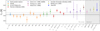 |
Fig. A.1. Individual photometric and spectroscopic temperature measures for HD 20 obtained in this work. On the abscissa either the photometric color or the spectral region that was used to deduce Teff is labeled. Different colors indicate the different scales and methods employed (see legend and main text for details). For each Teff that was deduced from a color index, the negligible effect of no reddening and twice the applied reddening (E(B − V) = 0.0149 mag, Schlafly & Finkbeiner 2011) is denoted by light-colored ranges behind the circles that are barely visible. The IRFM findings for HD 20 by Alonso et al. (1999b) and González Hernández & Bonifacio (2009) are shown together with the literature values by Barklem et al. (2005) and Gaia DR2. The finally adopted temperature and its error ( |

A.1.1. ATHOS – temperatures from Balmer lines
ATHOS16 (A Tool for Homogenizing Stellar parameters, Hanke et al. 2018) is a stellar parameter pipeline designed to acquire high-accuracy and high-precision stellar parameters from optical spectra of FGK stars. To that end, it employs flux ratios (FRs) of empirically defined wavelength ranges to compute the stellar parameters Teff, [Fe/H], and log g from dedicated analytical relations that have been trained on a large sample of benchmark stars. The strategy adopted is model-dependent only to the extent that a considerable fraction of the original parameters of the benchmark sample have been determined through modeling.
For Teff, the tool incorporates nine FRs involving the wings of two of the Balmer lines of neutral hydrogen, Hα and Hβ. Each of the nine FRs poses an independent measure of temperature. ATHOS was applied to all spectra containing Hα and Hβ, i.e. the UVES 580, MIKE, and HARPS spectra. In order to account for the substantial line broadening present in HD 20 (see Sect. 3.5), we provided ATHOS with an effective resolution,
under the assumption that rotational broadening behaves approximately Gaussian17. Here R0 denotes the instrumental resolving power of the input spectra. The mean temperature and its error for each of the nine relations are depicted in Fig. A.1, whereas the weighted mean Teff from all ATHOS results is 5194 ± 25 K, a temperature in good agreement with our adopted value. The latter low uncertainty is typical for the very high internal precision of ATHOS temperatures from high-S/N data. Nevertheless, it is important to bear in mind that the initial temperatures of ATHOS’ benchmark sample suffered from finite accuracy. Thus, we note an additional systematic error of 97 K (Hanke et al. 2018).
A.1.2. 3D NLTE modeling of Balmer lines
The classical spectroscopic approach of inferring Teff from Balmer lines relies on their theoretical modeling and comparison of the profile wings to observed spectra (Barklem et al. 2002). As a consequence, the approach is strongly model-dependent and prone to inaccuracies or unknowns in the attempts to reproduce real physical processes. To date, Amarsi et al. (2018) presented the most complex and potentially most accurate calculations of Balmer line formation in late-type stars involving 3D hydrodynamic atmosphere models and NLTE radiative transfer. The authors showed that departures from ordinary 1D LTE line formation can be substantial and their negligence could introduce temperature inaccuracies on the order of 100 K.
We took advantage of the extensive grid of 3D NLTE Balmer line models published by Amarsi et al. (2018) and closely followed their fitting scheme to deduce Teff for HD 20 from Hγ, Hβ, and Hα in the UVES spectra. In brief, for each profile, two 1D LTE spectra – one including metal lines and one considering only the H-lines – were modeled for the final parameters (Table 2) and a line list including all transitions for the respective synthesis range found in VALD. We used these two artificial spectra to define “clean” wavelength regions free from substantial metal absorption by requesting the residual deviation to result in a change of less than 30 K in the derived temperature. Furthermore, for Hα, we employed SkyCalc (Noll et al. 2012; Jones et al. 2013) to obtain a representative, synthetic telluric spectrum for the average observing conditions on Cerro Paranal and excluded all features above a threshold of 1% in absorption. Any of the remaining wavelength ranges with fluxes above 98% of the continuum flux were used to fit a linear continuum, while ranges of ≤98% of the continuum flux entered a χ2-minimization algorithm that interpolates between points of the Balmer model grid by employing cubic splines. For this purpose, all model parameters but Teff were kept fixed at their recommended values (Table 2). The resulting temperatures are 5260 K from Hγ, 5260 K from Hβ, and 5360 K from Hα. Here we caution against an over-interpretation of the deviation of the latter temperature because it amounts to less than one combined error margin and Hα is the least strong and least temperature-sensitive profile as can be seen in Fig. A.2. There the best-fit results are illustrated for all three profiles together with margins amounting to ±100 K, which we adopt as error estimate for individual measures from this method. The straight average Teff = 5293 ± 58 K is in good agreement with our independently determined, adopted value of 5246 K.
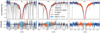 |
Fig. A.2. Teff fit results from fitting the wings of the Balmer lines Hγ (left), Hβ (middle), and Hα (right). Upper panels: observed spectra (gray) with the best-fit 3D NLTE models (5260/5260/5360 K) by Amarsi et al. (2018) and their error margins of 100 K depicted by red lines and blue areas, respectively. The wavelength regions used to obtain the continuum level are marked in blue, whereas orange lines highlight the parts of the spectrum that entered the χ2 minimization. Lower panels: residual spectrum. |
We would like to stress that, apart from model uncertainties, the accuracy of the outlined procedure is affected by non-linearities in the global continuum shape due to the blaze function, as has already been pointed out for UVES spectra by Amarsi et al. (2018). In fact, we see an asymmetric substructure in the residuals of Hβ that cannot be explained by model deficiencies. For the same reason the Balmer profiles in the MIKE spectrum were not used as they show slightly stronger persistent distortions after performing the above simple normalization scheme. The HARPS spectra only cover Hβ and Hα (5190 K and 5300 K, respectively) with no apparent residual substructure after normalization. However, the noise level considerably exceeds the error margin of 100 K, which is why we also excluded the HARPS spectrum from our consideration.
The treatment of normalization is one of the key advantages of the technique implemented in ATHOS over Balmer modeling: ATHOS does not rely on one global continuum for each Balmer profile, but rather computes its individual FRs from two wavelength regions that are spaced much less than the overall extent of the line. Indeed, this is based on the premise that between the two involved ranges the continuum stays constant. The narrow spacing, however, justifies the latter assumption. Moreover, typically, ATHOS provides four to five measures of temperature per Balmer line, such that any persistent effect induced by small-scale continuum variations can effectively be averaged out. This, on the other hand, would manifest itself in an increased relation-to-relation scatter, which is not observed for any of our HD 20 spectra.
A.1.3. Color – [Fe/H] – Teff calibrations
We further used the available photometry to compute Teff from several empirical relations in the literature. The first one was introduced by AAM99, who calibrated their analytical functions against a large sample of known [Fe/H] and Teff, which themselves were inferred from the infrared flux method (IRFM, e.g., Blackwell & Shallis 1977). Since HD 20 was part of their sample, we mention here their IRFM-based temperature of 5351 ± 84 K (Alonso et al. 1999b), which is slightly warmer compared to our adopted value. Unfortunately, most of the relations provided by AAM99 are not directly compatible with the photometry at hand, because AAM99 calibrated their relations for the infrared JHK bands in the Telescopio Carlos Sánchez (TCS) system instead of the 2MASS system. For this reason, we made use of a two-step conversion; first from the 2MASS to the CIT (California Institute of Technology) system as described in the supplemental material for the 2MASS mission18, and secondly to the TCS system adopting the transformations given by Alonso et al. (1994). Errors were propagated through all conversion steps, which poses the dominant source of error in the derived individual temperatures. We find a weighted average temperature of 5362 ± 52 K.
Barklem et al. (2005) report a result of 5445 ± 100 K using BVRCICJHKs photometry (b − y was not considered) by Beers et al. (2007) as well as the same color transformations and calibration relations. Despite having rejected that photometry (see Sect. 2.3), we attempted to reproduce their value from their photometry. To this end, for the R and I bands we applied the transformations given in Bessell (1983) to convert the magnitudes by Beers et al. (2007) to the Johnson ones. Nonetheless, using exactly the same averaging scheme – that is, dropping the strongest outliers in either direction, not considering b − y, and taking an unweighted mean19 – we cannot reproduce their rather hot value, but find 5270 K in accordance with our adopted estimate. Barklem et al. (2005) already noted generally warmer temperatures when comparing their sample to existing literature values and claimed the origin to be the usage of different reddening maps. Adopting their slightly higher extinction value of 0.017 only marginally increases our value by 5 K. We suspect two plausible reasons for the strong discrepancy, or a mixture thereof: If we neglected the erratum to AAM99 (Alonso et al. 2001) that cautions to invert the sign of the cross-term of colors and [Fe/H] in the calibrations, we would end up with temperatures that are on average higher by almost 200 K. Moreover, looking at Sivarani et al. (2004), who introduce the color transformations used by Barklem et al. (2005), we found that they transformed V − K colors to the Johnson system, while the AAM99 requires this color in the TCS system.
Another empirical calibration was introduced by Ramírez & Meléndez (2005) who revisited the IRFM temperature scale by AAM99 and provided updated relations (here we are only considering the scales for giants) for the filter systems given in Table 2. For the B − V color we would in principle have the necessary photometry, but the colors lie outside of the validity range of the relations. The weighted mean Teff from the remaining four colors involving the redder two 2MASS filters and Strömgren photometry is 5294 ± 79 K (rms), which is cooler (70 K) than the value obtained from AAM99 and hence more in line with the spectroscopic results.
The last photometric scale we consider is for the Strömgren color b − y, invented by Önehag et al. (2009). It is based on synthetic colors from MARCS model atmospheres. At 5518 ± 102 K, we find the derived temperature to be much hotter (∼250 K) than our adopted value.
Gaia DR2 provides temperature estimates for millions of sources based on Gaia colors alone, as described in Andrae et al. (2018). Although the authors note that due to several limitations their temperatures are impractical for studies of individual stars, for completeness, we mention their value of  K. Considering the small lower uncertainty, this again represents an unfeasibly high Teff.
A.2. ATHOS – [Fe/H] from flux ratios
ATHOS not only allows for the inference of Teff, but its FR-based method was also expanded to provide estimates for [Fe/H]. In total, there are 31 FRs involving Fe I lines that – together with the previously determined Teff – span hypersurfaces, which allow for [Fe/H] computations. The corresponding analytical relations where trained and fit on the same training sample as the temperature method. The metallicity labels were either extracted from the detailed studies of the Gaia benchmark stars (Jofré et al. 2014; Hawkins et al. 2016), or stem from a homogeneous analysis of Fe II lines in LTE (see Hanke et al. 2018, for details). For HD 20, we found [Fe/H] = −1.62 ± 0.06 dex from the median and rms scatter of all 31 FRs, respectively. This finding is in excellent agreement with our adopted [Fe/H] of −1.60 dex and therefore poses and independent validation.
A.3. The width of the Hα core as mass indicator
While the wings of the Balmer line Hα were used earlier to infer Teff, we will now address the usage of its line core to derive the stellar mass. Bergemann et al. (2016) have shown that even in the face of current, state-of-the-art modeling techniques, it is not possible to reliably synthesize this part of the line. However, adopting an empirical approach, the authors discovered a connection between the Hα core width and the stellar mass. The latter originated from CoRoT and Kepler asteroseismology.
We pursued the strategy outlined in Bergemann et al. (2016) and fit the blue profile wing (6562.0 Å < λ < 6562.8 Å) via the function
with free parameters f0 and WHα, and the central position of the line core λ0 = 6562.819 Å. From the width WHα, we then computed the mass parameter log10m/m⊙ using the relation given in Bergemann et al. (2016) and subsequently the surface gravity through inversion of Eq. (8). The involved solar reference values can be found in Table 2. As for Eq. (6), we computed the bolometric magnitude Mbol from the V-band photometry and BCV by AAM99. The measurements and results for individual spectra covering Hα are presented in Table A.1. The error in log g is largely governed by the uncertainty in the mass and for the gravity from this method we obtained log g = 2.17 ± 0.10 dex in line with our measurements based on NLTE ionization equilibrium and about 2σ lower than our asteroseismic finding. A plausible reason for this discrepancy may be found in the circumstance that, strictly speaking, HD 20 is about 250 K warmer than the upper validity bound for Teff in the calibration relation by Bergemann et al. (2016).
Stellar masses and log g from the core of Hα.
Appendix B: Abundance systematics
B.1. Instrument-induced versus other systematics
As has been pointed out by the referee, given our high-quality spectra gathered with three different instruments, it is possible to investigate the presence of systematics originating from the choice of different resolutions and fiber-fed (in case of HARPS) versus slit spectrographs (MIKE and UVES). To this end, we performed tests using lines of the species Ti II, Fe I, and Nd II that are distributed between 4000 Å and 6800 Å, which renders them accessible by all three instruments with only a few exceptions in the chip gaps. These three elements were chosen because they are on the one hand, representatives for the main groups of α, iron-peak, and neutron-capture elements and, on the other hand, they allow for measurements of a sufficient number of lines (in this case more than 20) that permit meaningful number statistics.
EWs for the sample of lines described above were measured in all three spectra using EWCODE. In the upper panels of Fig. B.1 we present the difference between measurements employing HARPS and UVES with respect to MIKE EWs. It is noteworthy that in principle the spread in this quantity is a convolution of both noise-induced errors from HARPS (UVES) and MIKE. However, in light of the substantially higher S/N of the MIKE spectrum at almost any wavelength, it appears safe to assume only a minor contribution due to noise in the MIKE spectrum. There are no obvious systematic trends or biases in the residuals, which leads us to the conclusion that for our analysis procedures of the star HD 20 the three spectrographs are entirely interchangeable without having to worry about introducing (additional) abundance systematics. The only notable difference is of a pure stochastic nature in the sense that HARPS EW residuals show larger spreads than UVES, which can be tied to the significantly lower S/N (see Fig. 1).
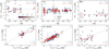 |
Fig. B.1. Comparison of EWs (upper panels) and deduced abundances (lower panels) obtained from the same lines that were measured with three different instruments. Panels are horizontally separated by the three representative chemical species (from left to right: Ti II, Fe I, and Nd II). Upper panels: residual EWs between HARPS (blue) and UVES (red) measurements with respect to the corresponding MIKE EWs as a function of wavelength. The lightness of the color stands for the measured EW in the MIKE spectrum as indicated by the color bars in the upper left panel. Lower panels: abundances from the MIKE spectrum are shown on the abscissas, whereas HARPS and UVES findings are given along the ordinates. In each panel the perfect one-to-one correlation is represented by gray dashed lines and the correlation coefficients computed for the samples are presented on the lower right. |
Once the EWs are propagated through the abundance analysis, it becomes obvious that noise is not the dominant source of error for the vast majority of lines when employing any of the tested instruments and their attributed S/N levels. This is illustrated in the lower panels of Fig. B.1, where individual abundances from lines measured in the HARPS and UVES spectra are depicted as a function of their MIKE counterpart. NLTE corrections were applied to Fe I and are expected to be negligible for the other two species. If spectrum noise were the sole reason for abundance errors the distributions would be completely uncorrelated and show ellipses that are aligned with the coordinate axes. Instead, we found strong correlations that imply governing systematic error components. We mention here possible origins for this observation to be uncertain oscillator strengths and/or shortcomings in the assumptions of one-dimensional and static atmospheres.
For Fig. B.2 we decoupled the systematic from the statistical component by performing line-by-line differential comparisons to the MIKE abundances. It is evident that the scatter in absolute abundances is hardly lower than 0.1 dex, while it is as low as 0.03 dex in the differential case for Fe I and the UVES/MIKE combination. The spread in absolute abundances motivates the floor abundance error of 0.1 dex employed throughout this work in those cases (n < 4) where the scatter could not be rigidly determined from the sample of lines themselves.
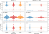 |
Fig. B.2. Violin plots of absolute (left) and line-by-line differential (right) abundances for the same representative elements as in Fig. B.1. Colors indicate spectrographs in the same way as in that figure with MIKE additionally being depicted in orange. Circles and vertical lines represent the median abundances, 15.9th, and 84.1th percentiles, respectively. The latter are furthermore printed at the bottom of each panel together with the number of involved lines, n. |
B.2. Impacts of model atmosphere errors
Here we present a detailed investigation of the propagation of errors on the key atmospheric parameters Teff, log g, [Fe/H], and vmic into the inferred individual stellar abundances (or upper limits) in LTE. To this end, eight model atmospheres were interpolated from the ATLAS grid, each denoting the departure of a stellar parameter from its optimal value by an amount dictated by our adopted errors (Table 2). These altered atmospheres were used to redetermine the abundances from all transitions measured in this work based on their EW. In those cases where spectrum synthesis was used, a converted EW corresponding to the determined abundance was initially calculated through the MOOG driver ewfind and the set of optimal atmospheric parameters. New average abundances were then derived using the median of all findings for one species. The resulting departures from the abundances listed in Table 4 can be found in Fig. B.3.
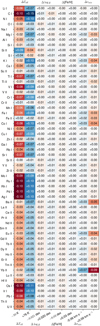 |
Fig. B.3. Change in elemental abundances log ϵ from individually varying the input model parameters by their error margins. Red and blue colors denote negative and positive residuals, respectively. The strength of the impact of an altered parameter (abscissa) on the elemental abundance (ordinate) is highlighted by the lightness of the color, where dark colors indicate strong departures. |
While the model metallicity can certainly be neglected as a factor of uncertainty, for the vast majority of elements, the model temperature appears to be the most critical parameter, in that changes induce the largest abundance deviations. Generally, the neutral species are more susceptible to Teff than their ionized counterparts. Abundance deviations of the ionized species of the neutron-capture elements do not exceed the 0.05 dex level, therefore highlighting the robustness of the resulting pattern against model uncertainties.
Interestingly, the overall trend of abundances correlating with temperature is reversed for Si II and S I, where an anti-correlation is seen. We further note that considerable departures reaching or even exceeding the 0.10 dex level were found for C, Mo to Ag, Os I, and Ir I. Both effects can be linked to the lower energy level of the transitions as we show in Fig. B.4. At the extreme end of temperature-related departures the lower level exclusively resides close to or at the ground level. In that regime, the number density is largely independent of temperature and the Teff affects exclusively the H− continuous opacity with its strong temperature gradient. This leads to a strengthening of lines and, in turn, lower abundances at fixed line strengths. With increasing χex the number density becomes susceptible to the Teff change and increasingly counteracts the effect of the lower H− opacity. Hence, the abundance departures are reduced. For the high-χex lines, the impact of the change in number density exceeds the opacity effect, which leads to the inverse temperature dependence seen in Fig. B.4.
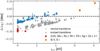 |
Fig. B.4. Individual abundance changes from lowering the model Teff by 50 K. Features from neutral species are shown in gray, whereas blue circles indicate ionized species. Highlighted in red and orange are the elements explicitly mentioned in the text. The manifold of CH lines used for synthesis and hence determination of the C abundance are not shown here. Their χex commonly resides around 0 eV. |
Variations in the stellar surface gravity have their strongest effect on abundances of ionized species, although the overall magnitude remains low at ∼ ± 0.01 dex. This can be understood in terms of gravity having a direct impact on the electron pressure which, in turn, determines the degree of ionization (Saha equation). Here our O I and S I transitions behave as if they were ionized.
Deviations from changing vmic exceed the 0.03 dex level in the mean abundances only for K I, Co I, Ba II, Eu II, and Yb II. The effect is limited to these species, as they show moderately strong lines with EWs of more than 80 mÅ and effects from microturbulence are limited to the higher line strength regime.
Appendix C: Additional table
Atomic transition parameters and abundances for individual lines.
All Tables
Comparison of abundances for HD 20 in common between Burris et al. (2000) and Barklem et al. (2005).
Median values and 68.2% confidence intervals for the stellar parameters from the posterior distributions for the three different likelihood functions (see main text for details).
Estimated fractional contributions from the r- and s-process for elements with Z ≥ 38 in HD 20.
All Figures
|
Fig. 1. S/N as a function of wavelength for the employed spectra of HD 20 from all three high-resolution spectrographs. Since the dispersion spacing between adjacent pixels varies among the instruments, we present the S/N per 1 Å. |
| In the text | |
|
Fig. 2. Comparison of literature time series for vhelio by Carney et al. (2003, gray-filled circles) and Hansen et al. (2015, blue-filled circles) to measurements from the three spectra employed throughout this study (see legend). The gray and blue dashed lines resemble the median values for the two reference samples. |
| In the text | |
|
Fig. 3. Power spectral density (PSD) for HD 20 based on TESS light-curve data. The thick black line depicts a smoothed version of the PSD (thin gray line) and the best-fit model is shown in red. The blue shaded area indicates the power excess, whereas individual model components are represented by thin blue and black dashed lines. |
| In the text | |
|
Fig. 4. Samples drawn from the posterior distribution of the stellar parameters (Eq. (2)). Shown are the three different approaches M1 (gray), M2 (red), and M3 (blue) with the darkness of the colors illustrating the local density as estimated from a Gaussian kernel density estimate. The sample sizes are 2 × 10⁴ and the adopted stellar parameters from method M3 (Tables 2 and 3) based on the median of the distributions are indicated using horizontal and vertical dashed lines. The correlation coefficients for pairs of two parameters in M3 are presented in the top left corner of each panel. The marginalized, one-dimensional distributions for the individual parameters are depicted by smoothed histograms at the top of each column. |
| In the text | |
|
Fig. 5. Diagnostic plot for spectroscopic ionization balance. Shown are the histograms of the Fe abundance distributions ([Fe/H] = log ϵ(Fe) − 7.50 dex) at the adopted gravity (log g = 2.24 dex from method M2, see Sect. 3.4) both in LTE (gray filled) and NLTE (blue) for Fe I and in LTE for Fe II (red). NLTE corrections for Fe II remain well below 0.01 dex and are therefore neglected here. Points with error bars and arbitrary ordinate offsets at the top of the panel denote the means and standard deviations for each of the distributions of the same color. |
| In the text | |
|
Fig. 6. Comparison of synthetic line shapes against the observed profiles in the UVES 580 spectrum for two representative Ti lines. Red spectra resemble 3D syntheses, while blue and orange colors indicate 1D syntheses with and without additional broadening. The instrumental profile (R = 66 230) was mimicked by convolution with a Gaussian kernel for all three types of synthesis. No rotational broadening was applied to the 3D syntheses. |
| In the text | |
|
Fig. 7. C abundance and 12C/13C from the CH G-band in the UVES 390 spectrum. Left panel: region around the two features that are dominated by 13CH, one of which is used to pinpoint 12C/13C (blue rectangle). The bluer feature at ∼4230 Å was not considered due to an unidentified blend (see main text). The observed spectrum is represented by black dots connected by gray lines and the best-fit synthesis (red) and its abundance error margin of 0.05 dex are depicted in blue, respectively. The dashed spectrum shows a synthesis without any C. Right panel: same as left panel but in the range used to constrain the C (CH) abundance. |
| In the text | |
|
Fig. 8. Two-dimensional representation of the MCMC sample used to fit log ϵ(C) and 12C/13C simultaneously including the marginal distributions. Median values and asymmetric limits are displayed by dashed lines. |
| In the text | |
|
Fig. 9. Same as right panel of Fig. 7, but for a synthesis of the NH-band at ∼3360 Å. A synthesis without any N is indicated by the black dashed curve. The blue error range corresponds to an abundance variation of ±0.10 dex. |
| In the text | |
|
Fig. 10. Synthesis of the Lu II line at 6221.9 Å. The red line represents the best abundance match with an error of 0.1 dex (blue shaded region). The broad range of HFS components for 175Lu from Lawler et al. (2009) are indicated by vertical orange lines at the top and have been taken into account for this synthesis. The impact of the negligence of HFS on the line shape is indicated by the blue line. |
| In the text | |
|
Fig. 11. Upper limit on Rb from the Rb I line at 7800.3 Å. The red model denotes the adopted upper limit of +1.52 dex, whereas blue lines are syntheses with Rb abundances successively increased by 0.2 dex. |
| In the text | |
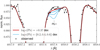 |
Fig. 12. Same as Fig. 11 but for the Pb I transition at 4057.8 Å and an upper limit of +0.37 dex. |
| In the text | |
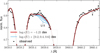 |
Fig. 13. Same as Fig. 11 but for the U II feature at 3859.6 Å and an upper limit of −1.21 dex. |
| In the text | |
|
Fig. 14. Comparison of CNO elemental abundances of mixed and unmixed stars with HD 20 shown in blue for comparison. Gray circles resemble the study by Gratton et al. (2000) while red triangles indicate the stars published in Spite et al. (2005, 2006). Two C-rich stars were excluded from the latter sample. Lower limits on 12C/13C are indicated by upward pointing arrows and the classification into mixed and unmixed stars according to the authors are represented by open and filled symbols, respectively. The red line in the lower panel mimics the linear relation between [N/O] and [O/H] for mixed stars as reported by Spite et al. (2005), whereas the dashed line extrapolates the same relation to higher values of [O/H]. |
| In the text | |
|
Fig. 15. Kiel diagram (upper panel) and Hertzsprung-Russell diagram (lower panel) with isochrones and helium burning tracks. HD 20’s position is depicted by a blue filled circle with error bars. Upper panel: the error on the gravity is smaller than the circle size. The red line represents a He-normal 11 Gyr isochrone at [Fe/H] = −1.60 dex, and [α/Fe] = +0.4 dex with age and metallicity error margins shown by orange and blue ranges. The RGB luminosity bump for this particular model at log L/L⊙ ∼ 2.0 is highlighted in the lower panel by an arrow and the label “LB”. The light blue curve is a model with the same parameters except for Y = 0.4. He-burning tracks for three different masses are shown by gray lines of different line styles with the stellar masses being indicated next to the respective tracks. |
| In the text | |
|
Fig. 16. Comparison of HD 20 (blue circle) to the metal-poor field star compilation (gray dots) by Roederer et al. (2014) and the red horizontal branch star HD 222925 (Roederer et al. 2018b, red circle). Dark blue circles and error bars indicate the result in LTE while the light blue circles indicate the NLTE-corrected ones. In the reference samples, corrections have been applied to O I, Na I, and K I. On the abscissa we show abundances from Fe II since these are less prone to departures from the LTE assumption (Sect. 3.3). |
| In the text | |
|
Fig. 17. Residual abundance pattern from O to Zn between HD 20 and HD 222925 after scaling by the difference in log ϵ(Fe II) of 0.13 dex. NLTE abundances were used for both stars for Na I and K I (red filled circles). |
| In the text | |
|
Fig. 18. Neutron-capture abundance pattern in LTE. Upper panel: HD 20’s heavy element abundances are indicated in blue. Shown in gray and red are abundances of the r-II star CS 22892−052 by Sneden et al. (2003) and the r-I star BD +17 3248 by Cowan et al. (2002) with updates from Cowan et al. (2005) and Roederer et al. (2010). The omitted Lu abundance for BD +17 3248 (see main text) is depicted in light red. Both patterns were scaled to achieve the overall best match to HD 20 in the entire considered range. The gray solid line denotes the solar-scaled r pattern from Sneden et al. (2008) and the best-fit AGB model (see text) is represented by dotted lines. Middle panel: residual pattern between HD 20 and the solar r pattern (gray line), CS 22892−052 (gray), and BD +17 3248 (red). Lower panel: residual pattern after mixing a contribution from BD +17 3248 with s-process material from the AGB yield model. |
| In the text | |
|
Fig. 19. Comparison of [hs/ls] and upper limit on [Pb/hs] for HD 20 against AGB s-process models of different initial masses. The value determined for HD 20 is indicated by blue horizontal lines and error margins, while models of Z = 0.0001 without rotation are shown in red. The adopted best-fit model with a rotation of 30 km s−1 is depicted in orange. For juxtaposition, we show i-process predictions for [hs/ls] from Hampel et al. (2016) for four different neutron densities, ni, in the upper panel using black dotted, dash-dotted, dashed, and solid lines (see legend). |
| In the text | |
|
Fig. 20. Estimated r- (right-hand scale) and s-fractions (left-hand scale) in HD 20 based on Eq. (10) with BD +17 3248 as proxy for an r pattern and the best-fit AGB model representing the s-enrichment site. Shown are only those elements that have a measured abundance in BD +17 3248. |
| In the text | |
|
Fig. 21. Comparison of the residual HD 20 pattern (purple, same as lower panel of Fig. 18) to the patterns of HD 94028 (red) and #10464 (green) after subtracting r + s and s contributions, respectively. The residual pattern for HD 94028 was determined following the procedure outlined in Sect. 5.2 in Roederer et al. (2016), whereas a Z = 0.0001, 2 M⊙ AGB model was assumed for the s-enrichment in #10464. |
| In the text | |
|
Fig. A.1. Individual photometric and spectroscopic temperature measures for HD 20 obtained in this work. On the abscissa either the photometric color or the spectral region that was used to deduce Teff is labeled. Different colors indicate the different scales and methods employed (see legend and main text for details). For each Teff that was deduced from a color index, the negligible effect of no reddening and twice the applied reddening (E(B − V) = 0.0149 mag, Schlafly & Finkbeiner 2011) is denoted by light-colored ranges behind the circles that are barely visible. The IRFM findings for HD 20 by Alonso et al. (1999b) and González Hernández & Bonifacio (2009) are shown together with the literature values by Barklem et al. (2005) and Gaia DR2. The finally adopted temperature and its error ( |
| In the text | |
|
Fig. A.2. Teff fit results from fitting the wings of the Balmer lines Hγ (left), Hβ (middle), and Hα (right). Upper panels: observed spectra (gray) with the best-fit 3D NLTE models (5260/5260/5360 K) by Amarsi et al. (2018) and their error margins of 100 K depicted by red lines and blue areas, respectively. The wavelength regions used to obtain the continuum level are marked in blue, whereas orange lines highlight the parts of the spectrum that entered the χ2 minimization. Lower panels: residual spectrum. |
| In the text | |
|
Fig. B.1. Comparison of EWs (upper panels) and deduced abundances (lower panels) obtained from the same lines that were measured with three different instruments. Panels are horizontally separated by the three representative chemical species (from left to right: Ti II, Fe I, and Nd II). Upper panels: residual EWs between HARPS (blue) and UVES (red) measurements with respect to the corresponding MIKE EWs as a function of wavelength. The lightness of the color stands for the measured EW in the MIKE spectrum as indicated by the color bars in the upper left panel. Lower panels: abundances from the MIKE spectrum are shown on the abscissas, whereas HARPS and UVES findings are given along the ordinates. In each panel the perfect one-to-one correlation is represented by gray dashed lines and the correlation coefficients computed for the samples are presented on the lower right. |
| In the text | |
|
Fig. B.2. Violin plots of absolute (left) and line-by-line differential (right) abundances for the same representative elements as in Fig. B.1. Colors indicate spectrographs in the same way as in that figure with MIKE additionally being depicted in orange. Circles and vertical lines represent the median abundances, 15.9th, and 84.1th percentiles, respectively. The latter are furthermore printed at the bottom of each panel together with the number of involved lines, n. |
| In the text | |
|
Fig. B.3. Change in elemental abundances log ϵ from individually varying the input model parameters by their error margins. Red and blue colors denote negative and positive residuals, respectively. The strength of the impact of an altered parameter (abscissa) on the elemental abundance (ordinate) is highlighted by the lightness of the color, where dark colors indicate strong departures. |
| In the text | |
|
Fig. B.4. Individual abundance changes from lowering the model Teff by 50 K. Features from neutral species are shown in gray, whereas blue circles indicate ionized species. Highlighted in red and orange are the elements explicitly mentioned in the text. The manifold of CH lines used for synthesis and hence determination of the C abundance are not shown here. Their χex commonly resides around 0 eV. |
| In the text | |
Current usage metrics show cumulative count of Article Views (full-text article views including HTML views, PDF and ePub downloads, according to the available data) and Abstracts Views on Vision4Press platform.
Data correspond to usage on the plateform after 2015. The current usage metrics is available 48-96 hours after online publication and is updated daily on week days.
Initial download of the metrics may take a while.