| Issue |
A&A
Volume 699, July 2025
|
|
|---|---|---|
| Article Number | A133 | |
| Number of page(s) | 34 | |
| Section | Interstellar and circumstellar matter | |
| DOI | https://doi.org/10.1051/0004-6361/202554096 | |
| Published online | 07 July 2025 | |
PDRs4All
XIV. Probing CH out-of-plane bending modes of PAH molecules in the Orion Bar with JWST
1
Department of Physics & Astronomy, The University of Western Ontario,
London
ON N6A 3K7,
Canada
2
Department of Physics, Durham University,
Durham
DH1 3LE,
UK
3
Institute for Earth and Space Exploration, The University of Western Ontario,
London
ON N6A 3K7,
Canada
4
Carl Sagan Center, SETI Institute,
339 Bernardo Avenue, Suite 200, Mountain View,
CA
94043,
USA
5
Leiden Observatory, Leiden University,
PO Box 9513,
2300
RA
Leiden,
The Netherlands
6
Astronomy Department, University of Maryland,
College Park,
MD
20742,
USA
7
Department of Astronomy, Graduate School of Science, The University of Tokyo,
7-3-1 Bunkyo-ku,
Tokyo
113-0033,
Japan
8
NASA Ames Research Center,
MS 245-6, Moffett Field,
CA
94035-1000,
USA
9
Institut des Sciences Moléculaires d’Orsay, Université Paris-Saclay,
CNRS, Bâtiment 520,
91405
Orsay Cedex,
France
10
Instituto de Física Fundamental (CSIC),
Calle Serrano 121-123,
28006
Madrid,
Spain
11
Space Telescope Science Institute,
3700 San Martin Drive,
Baltimore,
MD
21218,
USA
12
School of Physics, University of Hyderabad,
Hyderabad,
Telangana
500046,
India
13
Anton Pannekoek Institute for Astronomy, University of Amsterdam,
Amsterdam,
The Netherlands
14
Telespazio UK for ESA, ESAC,
E-28692
Villanueva de la Cañada,
Madrid,
Spain
15
IPAC, California Institute of Technology,
Pasadena,
CA,
USA
16
Instituto de Matemática, Estatística e Física, Universidade Federal do Rio Grande,
96201-900
Rio Grande,
RS,
Brazil
17
School of Physics and Astronomy, Sun Yat-sen University,
2 Da Xue Road,
Tangjia,
Zhuhai
519000, Guangdong Province,
China
18
Astronomy Department, Ohio State University,
Columbus,
OH
43210,
USA
19
Institut de Recherche en Astrophysique et Planétologie, Université Toulouse III – Paul Sabatier, CNRS, CNES,
9 Av. du colonel Roche,
31028
Toulouse Cedex 04,
France
20
Institut d’Astrophysique Spatiale, Université Paris-Saclay, CNRS,
Bâtiment 121,
91405
Orsay Cedex,
France
21
Department of Astronomy, University of Michigan,
1085 South University Avenue,
Ann Arbor,
MI
48109,
USA
★ Corresponding author: This email address is being protected from spambots. You need JavaScript enabled to view it.
Received:
10
February
2025
Accepted:
3
April
2025
Abstract
Context. The infrared universe is dominated by emission from polycyclic aromatic hydrocarbons (PAHs) observed as aromatic infrared bands (AIBs). JWST has produced a rich trove of information on these PAH signatures.
Aims. We aim to investigate the photochemical evolution of PAHs in photodissociation regions (PDRs), focusing on their molecular edge structures across key zones, including the H II region, the ionization front, the atomic PDR, the dissociation front, and the molecular PDR.
Methods. We utilized JWST’s MIRI-MRS observations of the Orion Bar for the PDRs4All JWST Early Release Science program. We investigated the spectral and spatial characteristics of 10–15 µm AIBs.
Results. The AIBs at 10.6, 10.8, 11.0, 11.2, 12.0, 12.7, 13.5, 14.0, and 14.2 µm share large-scale spatial morphologies, peaking in the atomic PDR and gradually declining with distance from the PDR surface. Correlations between the AIBs reveal that they are largely carried by PAHs. Profile variations and subcomponents of the 11.2 and 12.0 µm AIBs reveal a carrier that behaves independently of PAHs, which we attribute to very small grains (VSGs) and/or PAH clusters. We ascribe the 11.0 and 11.207 µm AIBs, part of the 12.0 µm AIB, and the 12.7, 13.5, and 14.2 µm AIBs to CHoop modes and discuss their hydrogen-adjacency assignments. We propose that the 10.6, 10.8, and 14.0 µm AIBs do not arise from CHoop modes. We derived the relative amounts of solo, duo, trio, and quartet CH groups to infer the molecular structures. These suggest that PAHs are dominated by solo and trio CH groups throughout the PDR. We attribute the decrease in duo and quartet CH groups relative to the solo CH groups toward the PDR surface to the effects of photolysis of the labile hydrogens.
Conclusions. The 10–15 µm AIBs are powerful probes of the PAH molecular structures. This study showcases the spatial and spectral variability in CHoop features due to photochemical processing of PAHs, and the differentiated spectral characteristics of PAHs and VSGs, in a prototypical PDR.
Key words: astrochemistry / techniques: spectroscopic / ISM: molecules / photon-dominated region (PDR) / infrared: ISM / ISM: individual objects: Orion Bar
© The Authors 2025
 Open Access article, published by EDP Sciences, under the terms of the Creative Commons Attribution License (https://creativecommons.org/licenses/by/4.0), which permits unrestricted use, distribution, and reproduction in any medium, provided the original work is properly cited.
This article is published in open access under the Subscribe to Open model. This email address is being protected from spambots. You need JavaScript enabled to view it. to support open access publication.
1 Introduction
Aromatic infrared bands (AIBs) are prominent broad spectral features in the infrared (IR) spectra emerging from diverse astrophysical regions, including: H II regions, planetary nebulae, young stellar objects, reflection nebulae, and the interstellar medium (ISM) (e.g., Gillett et al. 1973; Willner et al. 1977; Cohen et al. 1986; Genzel et al. 1998; Peeters et al. 2002). Aromatic infrared bands are also detected in nearby and distant galaxies, and are important tracers of the physical conditions in galactic environments (Spilker et al. 2023; Schroetter et al. 2024). Due to the ubiquity of these bands, the emitters of these features must be both resilient and omnipresent, thereby making them an important component of the ISM. The emission mechanism of AIBs is generally attributed to the IR fluorescence of polycyclic aromatic hydrocarbons (PAHs) – a family of large carbonaceous molecules with typically 50–100 carbon atoms (Tielens 2008). These molecules are composed of fused benzene rings, forming a honeycomb-like structure with hydrogen atoms decorating the aromatic rings at the edges. Excited upon absorption of interstellar photons, the PAH molecules relax through IR emission in their vibrational modes, which is detected as AIBs (Leger & Puget 1984; Allamandola et al. 1985). The AIBs exhibit variations in their peak positions, profile characteristics, and relative intensities from source to source and within individual sources (e.g., Peeters et al. 2002; Smith et al. 2007; Boersma et al. 2016; Chown et al. 2024). Spectral classification schemes group AIBs within classes (A, B, C, and D) based on their peak positions and profile shapes, which have been found to correlate strongly with the type of object the AIBs belong to (e.g., Peeters et al. 2002; van Diedenhoven et al. 2004; Matsuura et al. 2014; Sloan et al. 2014).
The 10–15 µm wavelength regime of the AIB spectrum harbors a plethora of features that are due to out-of-plane (CHoop) bending vibrations of the edge CH groups in PAHs. The number of adjacent hydrogen atoms on the peripheral rings of the PAH molecules determine the peak wavelengths of bands in this spectral region (Bellamy 1975; Hudgins & Allamandola 1999). Therefore, the 10–15 µm CHoop modes provide a crucial diagnostic tool to probe the molecular edge structure of PAHs (Hudgins & Allamandola 1999; Hony et al. 2001). In terms of nomenclature, a single CH group on the perimeter of a cyclic unit in the PAH molecule is termed a “solo” CH group, whereas two, three, and four adjacent CH groups per cyclic unit are termed “duo,” “trio,” and “quartet” groups, respectively. Theoretical studies have driven the assignments of the 10–15 µm AIBs to specific PAH CHoop modes. The dominant AIB in this spectral region is the 11.2 µm AIB, which is ascribed to solo CH vibrations in neutral PAHs (Allamandola et al. 1999; Hudgins & Allamandola 1999; Hony et al. 2001; Bauschlicher et al. 2008, 2009). Moreover, the 11.2 µm AIB comprises two distinct classes, A11.2 and B11.2, devised by van Diedenhoven et al. (2004). Class A11.2 peaks in the 11.20–11.24 µm range, displaying a less pronounced red wing relative to the band’s peak intensity, while class B11.2 peaks at ∼ 11.25 µm and shows a more pronounced red wing. The 11.0 µm band has been unequivocally attributed to solo modes in cationic species (e.g., Hudgins & Allamandola 1999; Hony et al. 2001). The 12.0 µm AIB is associated with duo CHoop mode, the strong 12.7 µm AIB with duo and trio modes, the 13.5 µm AIB with quartet CHoop mode, and the 14.2 µm AIB with out-of-plane vibrations of quintet CH groups (Hony et al. 2001; Bauschlicher et al. 2009). Together with theoretical predictions, laboratory-measured IR spectra of astronomically relevant PAHs support the interpretation of these 10–15 µm AIBs as CHoop modes in PAHs (e.g., Oomens et al. 2003; Bakker et al. 2011; Zhen et al. 2018).
Spectral characteristics and variability in the AIBs encode changes in the underlying populations of the carrier PAHs, in terms of their abundance, size, charge, and molecular structures, which are in turn coupled to the physical and chemical conditions of their host environments. Photo-processing of PAHs thus directly affects their observed spectral features. While the richness of spectral signatures of astronomical PAHs is well documented, limitations on the sensitivity and spatial and spectral resolutions of prior IR facilities (e.g., Spitzer-IRS and ISO/SWS) hinder our efforts to fully understand the photochemical evolution of these AIB carriers. The launch of the James Webb Space Telescope has heralded in a new and groundbreaking epoch of IR astronomy, and the unprecedented capabilities and sensitivity of its instruments are now allowing us to overcome this challenge.
The JWST Early-Release Science (ERS) Program PDRs4All1 has observed the nearby, nearly edge-on prototypical photodissociation region (PDR), the Orion Bar, and has obtained IR spectroscopic observations of the PDR with the highest-quality spatial resolution as of yet (Berné et al. 2022). Photodissociation regions are interstellar regions where far-ultraviolet (FUV: 6 eV < hv < 13.6 eV) photons drive the physical and chemical conditions of the neutral gas (Tielens & Hollenbach 1985). Their IR emission is dominated by emission in the AIBs. The PDRs4All program has elucidated, far more effectively than before, the characterizations and spectral variability of these AIBs in the Orion Bar (Chown et al. 2024; Peeters et al. 2024; Pasquini et al. 2024; Schroetter et al. 2024). We have taken advantage of these superb observations to investigate the 10–15 µm AIBs, their origin in PAH CHoop modes, and to derive details of molecular structures of the photo-processed PAHs dwelling in the Orion Bar PDR.
We describe the noteworthy characteristics of the Orion Bar in Sect. 2. Details of the observations and data reduction are given in Sect. 3. The methodologies for continuum estimation and surface brightness measurements are described in Sect. 4. We present the observational characteristics, the relationships of the AIBs, and the results of a principal component analysis (PCA) of the surface brightnesses of the AIBs in Sect. 5. We discuss the spectroscopic assignments for the 10–15 µm AIBs in Sect. 6.1, and the implications for the PAH molecular edge structures and related photo-processing in Sect. 6.2. We discuss evidence of another population of carbonaceous AIB carriers, the very small grains (VSGs), in the Orion Bar in Sect. 6.3. Finally, we summarize the results of this study in Sect. 7.
2 The Orion Bar
The Orion Bar is a strongly illuminated escarpment of the Orion Molecular Core 1 (OMC-1) within the Orion molecular cloud complex, which is the closest site of ongoing massive star formation to us2. In front of OMC-1 lies the renowned, prototypical H II region, the Orion Nebula (M42). The inner region of this dense, ionized gaseous nebula is powered and sculpted by the ultraviolet (UV) radiation and mechanical feedback from the compact Trapezium cluster of massive stars. The most massive and brightest star in this cluster is the O7V-type star θ1 Ori C with Te f f = 38 950 K (Sota et al. 2011; O’Dell et al. 2017), which resides at the heart of the Orion Nebula (Bally 2008; Pabst et al. 2019). The “Bright Bar,” commonly known as the “Orion Bar,” is a highly irradiated PDR located at the interface of the molecular cloud and the surface of the H II region in the Orion Nebula, and has been well studied (e.g., Tielens et al. 1993; Pellegrini et al. 2009; Goicoechea et al. 2016). The Orion Bar is strongly illuminated by the stellar UV radiation from θ1 Ori C (Elliott & Meaburn 1974; Werner et al. 1976; O’Dell et al. 2020). Peeters et al. (2024) derived the maximum strength of the FUV radiation field, G03, impinging on the Orion Bar to be between 2.2–7.1 × 10⁴ with a median value of 5.9 × 10⁴.
The Orion Bar is viewed nearly edge-on and displays physical and chemical stratification of a typical PDR, which has been spatially resolved by JWST NIRCam, NIRSpec, and MIRI imaging and spectroscopic observations (Habart et al. 2024; Peeters et al. 2024; Chown et al. 2024; Van De Putte et al. 2024). As evident in the schematic view of the Orion Bar shown in Fig. 1, the ionization front (IF), located at a physical distance of 0.27 pc from θ1 Ori C, marks the separation of the edge of the H II region and the surrounding molecular cloud. The PDR begins just beyond the IF, where FUV photons with energies below 13.6 eV pervade the molecular cloud, the hydrogen gas transitions from ionized to neutral state, and dust and gas temperatures drop. The first layers of the PDR are neutral and predominantly atomic: [H] > [H2] ≫ [H+]. Absorption of incident FUV radiation by PAHs results in ejection of photoelectrons which are responsible for heating the warm and moderately dense gas ((5–10) × 104 cm−3) of the region (Tielens et al. 1993; Bakes & Tielens 1994). The gas remains atomic until the intensity of the penetrating FUV photons is sufficiently attenuated and the gas becomes mostly molecular. This marks the beginning of the molecular PDR. The H2 emission exhibits several ridges at increasing distances from the IF and roughly parallel to the IF. In the MIRI FOV, we observe three dissociation fronts (DFs: DF 1, DF 2, and DF 3). DF 1 and DF 2 are thin, dense filaments trapping the H2 dissociation front whereas DF 3 is the surface of a molecular clump (Goicoechea et al. 2025). We refer the reader to Habart et al. (2024), Peeters et al. (2024), and Goicoechea et al. (2025) for details of the geometry and large-scale stratification of the Orion Bar PDR.
The Orion Bar presents itself as an ideal environment for the study of the mid-IR emission from PAHs. The stratified edge-on geometry of the Orion Bar poses an advantage of investigating the effects of UV radiation on the population of PAHs and variations in their IR spectral signatures, across increasing distances from the ionizing source and decreasing local FUV radiation field. Leveraging the close proximity of the Orion Bar and its observations at an unprecedented high spatial resolution by the JWST, allows for investigations of the photo-processing of PAHs in the Orion Bar at the fine physical scales at which they typically occur. As an intensively studied, archetypal PDR, the Orion Bar is a rich astronomical laboratory, poised for JWST to probe and offer unparalleled insight into its physico-chemical landscape and molecular composition.
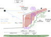 |
Fig. 1 Schematic view of the Orion Bar. Figure adopted from Peeters et al. (2024). |
3 Observations
Targeted by the JWST Early Release Science (ERS) program “PDRs4All: Radiative Feedback from Massive Stars”4 (Berné et al. 2022, ID: 12885; PIs: O. Berné, E. Habart, E. Peeters), the Orion Bar was observed by the JWST MIRI Medium Resolution Spectroscopy (MRS) Integral Field Unit (IFU) instrument (Wright et al. 2015; Wells et al. 2015; Wright et al. 2023; Argyriou et al. 2023) on 30 January 2023 (see Fig. 2 for the field of view (FOV)). The MIRI-MRS data spans the wavelength range of 4.90–27.90 µm at a spectral resolution of R ∼ 1500–3500. The MIRI-MRS data were re-reduced using version 1.11.1 of the JWST pipeline and JWST Calibration Reference Data System (CRDS) context 10976. Post-processing of the data resulted in three-dimensional (two spatial dimensions and one spectral dimension) data cubes for each of the four MIRI channels and their three sub-bands (short, medium, and long). The 12 sub-band cubes were stitched together to produce the final spatiospectral mosaic, used in this paper. Details of the observations, data reduction and the stitching algorithm are available in Chown et al. (2024) and Van De Putte et al. (2024). The MRS spectral leak at 12.2 µm cannot be corrected in spectral cubes or extracted spectra of extended sources. However, the contribution at 12.2 µm (a few percent of the specific surface brightness at 6.1 µm) is less than 2.5% of the specific surface brightness at 12.2 µm and as such will not influence our results. While we applied our analysis to every spaxel in the mosaic, we only considered every other spaxel in the correlation plots. Analysis on a spaxel basis may carry some problems due to the undersampling of the PSF (Law et al. 2023). However, we do not observe significant differences between spectra extracted from individual spaxels and those extracted from 2 × 2 spaxels.
Throughout our analysis, we also made use of the five MIRI “template spectra” extracted using key extraction apertures in the JWST NIRSpec IFU mosaic of the Orion Bar, seen in Fig. 2 (see also Fig. 2 of Peeters et al. 2024). These templates represent the prominent “phases” of the Orion Bar PDR: the ionized (H II) region, atomic (H I) region, and three bright H2 dissociation fronts. These template spectra and the zones of the PDR structure that they characterize are extensively discussed in Peeters et al. (2024). Hereafter, these template spectra are labeled as: H II region, atomic PDR, and DF 1, DF 2, DF 3 for the three H I/H2 dissociation fronts. The JWST observations in the line of sight toward the Orion Bar include two externally irradiated protoplanetary disks or “proplyds,” 203-504 and 203-506 that are highlighted in Fig. 2.
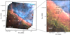 |
Fig. 2 Composite JWST NIRCam image of the Orion Bar. The JWST-MIRI/MRS IFU FOV is overlaid in white, and the spectral extraction apertures for the five template spectra are indicated with labels and black boxes in the right panel. The red, green, and blue colors encode the F335M (the 3.3 µm AIB), F470N-F444W (H2 emission), and F187N (Paschen α emission), respectively Habart et al. (2024). The ionizing source for the Orion Bar, θ1 Ori C, is represented by the ⋆ symbol on the top right edge of the left panel. In the right panel, the two proplyds 203-504 and 203-506 are shown through black circles, and the dashed black line indicates the cut across the MIRI mosaic (position angle, PA, of 155.79°). This figure is adapted from Chown et al. (2024), with permission. |
4 Methodology
To characterize the trends in spatial variation and correlations between the strengths of the AIBs observed in the Orion Bar, we adopted the following methodology of estimating the continuum and measuring the surface brightnesses of the bands.
4.1 Continuum estimation
The AIBs in the 10–15 µm spectra are perched atop a rising dust continuum and a smoothly varying, broad plateau. To characterize these AIBs, we determined a local spline continuum to exclude the emission from other contributors in the following way. We selected pairs of adjacent wavelengths between 9.1–10.3 µm and 12.2–15.4 µm. For each such wavelength pair, a wavelength anchor was placed at its average value and its specific surface brightness was taken to be equal to the average of the specific surface brightnesses in this wavelength range. In addition, we added one anchor at 11.695 µm. As shown in Fig. 3, the cubic spline was then interpolated between all the anchor points, and taken to be the estimate of the local continuum which was then subtracted from each spaxel of the data cube. For completeness, we also measured a global continuum, which excludes the 10–15 µm plateau (Fig. 3), which is utilized later in Sect. D.67.
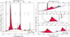 |
Fig. 3 Left: AIB template spectrum in the 10–15 µm region emergent from the Orion Bar atomic PDR. The blue curve indicates the underlying local continuum (dust continuum + plateau), the orange curve indicates the global continuum, the black circular markers are placed at the anchor points used to estimate the continuum, and the vertical solid blue lines indicate the nominal AIBs at 11.0, 11.2, 12.0, 12.7, and 13.5 µm, and the weakest AIBs at 10.6, 10.8, 14.0, and 14.2 µm, which are each shaded in red. Right: closer look at the weak AIBs, where the vertical dotted markers indicate the positions of the atomic and H2 lines. Previously observed bands at 10.6, 12.0, 13.5, and 14.2 µm are shaded in red. We observe emergence of weaker, adjacent features to the 10.6 and 14.2 µm AIBs at 10.8 µm and 14.0 µm, respectively, which are marked by the hatch pattern. |
4.2 Surface brightness measurements
Prior to measuring the integrated specific surface brightnesses, hereafter referred to as “surface brightnesses,” of the 10–15 µm AIBs, we removed several unresolved spectral lines present and identified by Van De Putte et al. (2024). Spectra in this wave-length region of interest include several H I recombination lines from the nl = 9 and nl = 10 series, several He I lines and the metal ion [Ni I], [S IV], [Ne II], and [Cl II] lines. The width of the wavelength range over which each line was removed was determined based on the relative strength of the peak specific surface brightness and the local continuum’s specific surface brightness; that is, a greater line strength relative to the continuum warranted data points over a larger wavelength range to be removed. A linear interpolation was then performed to generate data points over these line-removed windows.
The surface brightnesses for the AIBs [W m−2 µm −1 sr−1] were measured through Newton-Cotes-based numerical integration of the line-removed, continuum-subtracted spectra, over the selected integration windows. These integration wavelength windows were determined by inspecting the spectral features in the atomic PDR template spectrum and are highlighted in red in Fig. 3. We applied a simple de-blending between the weak 11.0 µm and the prominent 11.2 µm AIB, where the integration region for the 11.0 µm AIB is taken to be 10.9–11.1 µm, while that for the 11.2 µm AIB is 11.14–11.6 µm. This choice of integration limits results in an overestimation of the 11.0 µm surface brightnesses by up to 20% compared to a Gaussian-based deblending of the 11.0 and 11.2 µm AIBs performed by Peeters et al. (2017) and Schefter et al. (in prep.). The 12.7 µm complex was measured over the 12.2–13.1 µm range. We found that the 14.2 µm AIB profiles can be modeled well through Skewed Gaussian models. Thus, we opted to measure the 14.2 µm AIB using the SkewedGaussianModel from the lmfit package for Python, keeping the parameters of center (µ), standard deviation (σ) and skewness (γ) fixed, as below:
![Mathematical equation: \[\begin{array}{*{20}{l}}{f(x;A,\mu = 14.168,\sigma = 0.089,\gamma = 2.564) = \frac{A}{{\sigma \sqrt {2\pi } }}{e^{ - {{(x - \mu )}^2}/\left( {2{\sigma ^2}} \right)}}}\\{\,\,\,\,\,\,\,\,\,\,\,\,\,\,\,\,\,\,\,\,\,\,\,\,\,\,\,\,\,\,\,\,\,\,\,\,\,\,\,\,\,\,\,\,\,\,\,\,\,\,\,\,\,\,\,\,\,\,\, \times \left[ {1 + {\rm{erf}}\left( {\frac{{\gamma (x - \mu )}}{{\sigma \sqrt 2 }}} \right)} \right],}\end{array}\]](/articles/aa/full_html/2025/07/aa54096-25/aa54096-25-eq1.png)
where erf is the error function. We set the values of the fixed parameters (center (µ), standard deviation (σ) and skewness (γ)) to those of the fitting result for this AIB in the spectrum for the atomic PDR, where it is the strongest in peak specific surface brightnesses relative to other template spectra.
For our analysis, we masked out unreliable pixels at the NW/SE edges of the MIRI-MRS mosaic and pixels covering the two bright protoplanetary disks 203-504 and 203-506 in the mosaic (see Fig. 2). Additionally, following the strategy of Peeters et al. (2017), the signal-to-noise ratios (SNRs) of the AIBs were estimated as
![Mathematical equation: \[{\rm{SNR}} \approx \frac{{{{\rm{I}}_{{\rm{AIB}}}}}}{{{\rm{rms}} \times \sqrt {\rm{N}} \times {\rm{\Delta }}\lambda }},\]](/articles/aa/full_html/2025/07/aa54096-25/aa54096-25-eq2.png)
where IAIB is the surface brightness of an AIB in units of W m−2 sr−1, rms is the root-mean-square estimate of the noise determined from a featureless portion of the spectrum in units of W m−2 sr−1 µm−1, Δλ is the wavelength bin size contingent on the spectral resolution, and N is the number of spectral wavelength bins in a given AIB.
5 Results
We report the detection of a cohort of AIBs in the 10–15 µm (∼ 1000–667 cm−1) regime in Sect. 5.1. We present spatial maps of the surface brightnesses of the AIBs, and discuss trends in their spatial distributions in Sect. 5.2. We investigate the diversity of variations within the nominal 11.2 µm, 12.7 µm and 12.0 µm AIB profiles and present decompositions to analyze these AIBs in Sects. 5.3, 5.4, and 5.5, respectively, followed by an overview of the spectral variations observed for the 13.5 µm AIB in Sect. 5.6. We discuss notable correlations observed between the AIBs and their origin in PAH CHoop modes in Sect. 5.7. Lastly, the results of a PCA of the AIBs in this study are presented in Sect. 5.8.
5.1 Spectral inventory
Fig. 3 showcases the 10–15 µm AIBs that arise in the atomic PDR template of the Orion Bar. The nominal strong AIB at 11.2 µm dominates this spectral region. Its distinctly asymmetric profile has a steep blue rise and a gentle, broad red wing, displaying two notable components within: the first at 11.207 µm and the second at 11.25 µm (Chown et al. 2024; Pasquini et al. 2024). Chown et al. (2024) show that the 11.2 µm AIB in the Orion Bar shifts from class B11.2 in the molecular PDR toward class A11.2 in the atomic PDR. The well-known AIB at 11.0 µm conjoins with the blue shoulder of this 11.2 µm AIB. The 11.2 µm AIB is followed in intensity by the moderately strong 12.7 µm AIB. The 12.7 µm AIB complex exhibits a rich profile, comprising several terraces in its blue wing that are indicative of multiple blended subcomponents. Left-adjacent to the 12.7 µm complex we observe a weaker, asymmetric AIB at 12.0 µm, with a red tail. On the onset of the CHoop wavelength region, we identify a set of two neighboring broad, weak AIBs at 10.6 µm and 10.8 µm. The 10.6 µm AIB exhibits a blue extended wing, while its redder, slightly asymmetric companion at 10.8 µm, blends into it. At the end of the CHoop wavelength region lie AIBs at 13.5 µm, 14.0 µm, and 14.2 µm. The 13.5 µm AIB is asymmetric and skewed toward the shorter wavelengths. The 14.0 µm and 14.2 µm AIBs are slightly asymmetric, with the profile of the latter exhibiting a stronger left skew. Thus, the profiles of the AIBs in this regime predominantly display asymmetry through tails. These AIBs vary in profiles across the key zones of the Orion Bar PDR, as already demonstrated by Peeters et al. (2024), Chown et al. (2024), Pasquini et al. (2024), and Schroetter et al. (2024).
5.2 Feature morphologies
Spatial-spectral maps are a vital tool to investigate the spatial distribution of emission within complex AIBs. We present the spatial distribution maps and the radial profiles of the AIB surface brightnesses in Figs. 4 and 5, respectively. All radial profiles are measured along the cut across to the Orion Bar, visible in Fig. 2. We emphasize that we only discuss the AIB behavior in the Orion Bar, which excludes the H II region, since the Bar’s edge-on structure allows for a systematic investigation of the influence of the decreasing FUV field on the AIBs. We do provide the correlation plots, shown in the main text of the paper, for all spaxels in the mosaic (i.e., including the H II region) in Appendix F.
The following trends are shared by the spatial behavior of all the AIBs in our cohort. Peeters et al. (2024) find that the AIB emission – as characterized by the sum of all AIB components in the 3.2–3.7 µm range – from the H II region originates from the background face-on PDR, OMC-1 and increases dramatically across the IF. This marks the surface of the Orion Bar PDR. The AIB emission is strongest in the atomic PDR of the Orion Bar, near the IF, where the strong FUV radiation field aids in the excitation of the AIB carriers and subsequent relaxation. We observe similar spatial trends for the AIBs under study. Their emission peak near the IF in the atomic zone, and display smaller-scale structures therein, as is the case for the overall AIB emission (Peeters et al. 2024). Spatially, the regions of these pronounced emissions appear either in the form of ridges or in the form of two or more extended “lobes,” which are described in detail later in this section. There is a smooth decrease in the surface brightnesses of all AIBs with distance from the IF. Peeters et al. (2024) notice that the AIB emission reaches local maxima near the three H2 dissociation fronts, but these maxima are slightly displaced from the DFs toward the south. Such localized increases in emission strengths are most pronounced near DF 3 for the 10.8, 11.2, 12.0, and 13.5 µm AIBs (Fig. 5).
On top of this overall large-scale behavior, the AIBs display small-scale structure and variations. We discuss details of these small-scale structures and variations compared to the distributions of the main AIBs at 11.2 µm and 12.7 µm. The spatial anatomy of the strong 11.2 µm AIB displays most strikingly the prominence of AIBs in the atomic PDR. The brightest 11.2 µm signatures occur in three distinct structures: one bright limb located closest and parallel to the IF, which protrudes from the south-western long edge of the map, labeled “C,” and two other narrow concentrations, indicated by “A” and “B” in the atomic PDR (Fig. 4). The surface brightness of the 11.2 µm AIB, which tapers off toward the end of the atomic PDR, increases slightly at DF 1 and DF 2, and most notably at DF 3 (Fig. 5). The anatomy of the second strongest AIB in this wavelength regime at 12.7 µm, is similar to that of the 11.2 µm AIB. The 12.7 µm AIB exhibits three bright structures at roughly the same positions as A, B and C, but differing in sizes from the structures for the 11.2 µm AIB.
The 11.0 µm AIB is an order of magnitude weaker in strength than the 11.2 µm AIB. The peak 11.0 µm emission occurs in two distinct spatial structures that are co-spatial with the A and B lobes showing enhanced 11.2 µm AIB emission. These structures appear more extended in the 11.0 µm AIB – a result of the chosen integration method for the 11.0 µm AIB (Sect. 4.2).
The morphology of the 12.0 µm AIB emission in the atomic PDR most prominently differs from that of the 11.0, 11.2 and 12.7 µm AIBs. The 12.0 µm AIB emission peaks at two distinctively bright regions in the atomic PDR, one of which is co-spatial with enhanced 11.2 µm AIB emission in region C, and the other we label “D.” Figure 5 shows that, in comparison with the 11.2 and 12.7 µm AIBs, the 12.0 µm AIB experiences an amplification of its surface brightnesses at the three DFs, and most distinctly in DF 3.
We observe similar spatial trends in emission arising from the 13.5 µm AIB as for the 12.0 µm AIB. The areas of maxi-mal surface brightness for the 13.5 µm AIB align spatially with those for the 12.0 µm AIB in the atomic PDR. There exists slight enhancements in the surface brightnesses of the 13.5 µm AIB in DF 3. Per Fig. 5, these increases at the DFs are stronger for the 12.0 µm AIB than those for the 13.5 µm AIB.
The 10.6 µm and 10.8 µm AIBs present a similar morphology. Due to the weakness of these AIBs, in particular of the 10.8 µm AIB which is overall an order of magnitude weaker in strength than the 10.6 µm AIB, their maps appear less smooth compared to those of the stronger bands8. The strongest 10.6 µm emission is confined to a narrow ridge in the atomic PDR parallel to the IF, which seems to bridge the surfaces of regions A and C of enhanced 11.2 µm emission. This ridge-like structure is similar to that observed for the O I 1.317 µm line as seen in Peeters et al. (2024), albeit it appears deeper into the atomic PDR than the O I emission, which peaks just beyond the IF.
Finally, we state the morphologies of the two reddest companion AIBs located at 14.0 µm and 14.2 µm. Although the measurements of the 14.0 µm AIB are especially compromised by the continuum estimation, its spatial morphology resembles those of the other AIBs, particularly the stronger, neighboring AIB at 14.2 µm. Substantial spectral emission in these bands is limited to the atomic PDR. Most noticeably, the 14.2 µm AIB exhibit peak emission in the spatial structures A and B, similar to the 11.0 µm and 11.2 µm bands, but these emissions are much more broadly distributed. Similar as the 11.0 µm AIB, there is an absence of prominent 14.0 µm and 14.2 µm emission within region C which displays enhanced 11.2 µm emission.
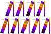 |
Fig. 4 Spatial variation in the surface brightnesses of the 10–15 µm AIBs in the Orion Bar PDR, in units of W m−2 sr−1. θ1 Ori C is located toward the top right of each map (see Fig. 2). For each map, the range of the corresponding color bar is set between 0.5% and 99.5% percentile level for the data, while zero pixels, edge pixels, and pixels covering the two proplyds, indicated by the black circles, are masked out. The contours trace peak emission for the 11.0 µm AIB (white), the 11.2 µm AIB (teal), and the specific AIB shown in the panel (black). The black letters in selected panels label the most notable structures, which are discussed in the text. The rectangular apertures of the template spectra for the H II region, atomic PDR, DF 1, DF 2 and DF 3, from top to bottom, are shown in white and the solid white lines delineate the IF and the three dissociation fronts, DF 1, DF 2 and DF 3. |
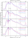 |
Fig. 5 Normalized surface brightnesses as a function of distance to the IF (0.228 pc or 113.4′′ from θ1 Ori C) along a cut crossing the mosaic (see Fig. 2 for the location of the cut). Normalization factors are listed in W m−2 sr−1 in parentheses for each surface brightness. As the cut is not perpendicular to the IF and distances are given along the cut, a correction factor of cos(19.58°)=0.942 needs to be applied to obtain a perpendicular distance from the IF. The vertical dash-dotted lines indicate the position of the IF, DF 1, DF 2, and DF 3, respectively, from left to right, where the DFs are defined by the maximum intensity of H2 emission (Peeters et al. 2024). The vertical dashed lines indicate the location of the proplyds 203–504 (left) and 203–506 (right). |
5.3 Investigating the 11.2 µm AIB
The 11.2 µm AIB profile observed in the Orion Bar is diverse in its spectral characteristics and reveals two prominent subcomponents centered at 11.207 µm and ∼ 11.25 µm (Fig. 6). Chown et al. (2024) conclude that these are two independent components given the variation in the relative strengths of these two components across the five template spectra. In particular, the peak of the first component (11.207 µm) occurs in the atomic PDR, the H II region and DF 1, whereas the second component (11.25 µm) peaks at DFs 2 and 3 (Chown et al. 2024). Pasquini et al. (2024) has employed a clustering-based unsupervised machine learning algorithm to analyze the variation in AIBs across the Orion Bar, revealing that the carriers of the two components of the 11.2 µm AIB are indeed independent. Thus, in addition to measuring the emission of the canopying 11.2 µm profile across the mosaic, we performed a decomposition of this profile to analyze the behavior of these two subcomponents, hereafter referred to as “component 1” and “component 2.” We also note the presence of an additional peak at ∼ 11.22 µm in the profiles (see Fig. 6), signaling a third component within the 11.2 µm AIB, albeit it is difficult to extract and measure. We present the spectral decomposition of this band in Sect. 5.3.1 and relationships of its components with the 11.0 µm AIB in Sect. 5.3.2.
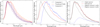 |
Fig. 6 Left: Normalized 11.2 µm profiles illustrating the spectral diversity. Middle: The normalized profile for the primary component representative of the narrowest 11.2 µm profiles emergent in the atomic PDR (belonging to class A11.2), the “transitional profile” of the broadest 11.2 µm profiles in DF 3 (belonging to class B11.2) and the profile of the secondary component used in the 11.2 µm AIB decomposition. Right: Linear combination fitting for the 11.2 µm profile of a spaxel from beyond DF 3. The weighted component 1 and component 2 profiles are the primary (11.207 µm) and secondary (11.25 µm) subcomponents. |
5.3.1 Decomposition of the 11.2 µm AIB spectral profiles
To investigate the two 11.2 µm components in the Orion Bar spectra, Pasquini et al. (2024) determined their spectral profiles from the average profiles for each of the four clusters they found when applying a clustering technique on the 11.2 µm profiles across the mosaic. Specifically, these authors assigned component 1 to the cluster profile with the smallest full width at half maximum (FWHM). This profile belongs to class A11.2. Next, these authors obtained the spectral profile of component 2 by taking the broadest cluster profile (which belongs to class B11.2) and subtracting a scaled component 1. They show that the spectral profiles of the remaining two clusters were well fit by linear combinations of both derived components. Initially, we performed a similar decomposition on the 11.2 µm spectral profiles at each spaxel; that is, we linearly combined the component profiles from Pasquini et al. (2024) to fit the 11.2 µm profiles over the 10.9–11.63 µm range. While effective at large, this linear decomposition results in a negative coefficient for component 2 for several spaxels in the atomic PDR, indicating that these 11.2 µm profiles are narrower than that of component 1 from Pasquini et al. (2024). As the profiles of components 1 and 2 from Pasquini et al. (2024) are generated from the average spectra for two clusters, each encompassing a large spatial area of the mosaic (the total mosaic was split up in four clusters total), they are unable to account for variations in the 11.2 µm profiles on the smallest spatial scales. Consequently, we performed the following revision on this decomposition method of the 11.2 µm profiles and measurements of the 11.207 µm and 11.25 µm components.
We reconstructed each spaxel’s 11.2 µm profile, normalized to the peak surface brightness over the 11.14–11.6 µm region, through a linear combination of two profiles representing the 11.207 µm and 11.25 µm components (components 1 and 2, respectively). The profile of component 1 is taken to be the average of a few of the narrowest class A11.2 profiles in the atomic PDR. To obtain component 2, we first averaged a few of the broadest class B11.2 profiles in DF 3, termed the “transitional” profile. These class B11.2 profiles in DF 3 profiles have the broadest FWHMs, as measured by Schefter et al. (in prep.). We scaled component 1 to fit within this transitional profile. This scaled component 1 profile was then subtracted from the transitional profile to produce the profile for component 2. We notice that the steep blue ascent of the transitional profile is not well fit. This is due to the fact that the PAH size is smaller in DF 3 compared to the atomic PDR resulting in a less steep blue wing in DF 3 (Chown et al. 2024, Schefter et al., in prep.). As we keep the profile of component 1 fixed, such a change in slope is not represented. Hence, we set the values of the component 2 spectral profile from 11.14–11.2 µm to zero. Figure 6 displays the profiles used for the two components. A linear combination of these two component profiles was then performed to fit the 11.2 µm profile at each spaxel (as is illustrated in Fig. 6). The specific surface brightnesses of the weighted component profiles were integrated to obtain the surface brightnesses for the 11.207 µm and 11.25 µm components. As is evident in Fig. 7, with the exception of spaxels in the atomic PDR that are similar to the component 1 profile, we were able to extract the emission of both the 11.207 µm and 11.25 µm components for the 11.2 µm spectral profiles across the mosaic.
Figs. 7 and 8 display the spatial maps and the surface brightnesses of the 11.2 µm AIB and its 11.207 µm and 11.25 µm components as a function of distance from the IF. The 11.207 µm component is the primary contributor to the aggregate 11.2 µm AIB (see also Fig. 6). Overall, the spatial signatures of the 11.207 µm component closely resemble those of the 11.2 µm AIB. However, the 11.207 µm component’s emission declines much faster across the DFs than the 11.2 µm AIB (Fig. 8).
The map of the 11.25 µm component presents a unique narrative. The following observations are also supported by the radial profiles presented in Fig. 8. The absolute surface brightness of the 11.25 µm component does indeed reach its zenith in DF 2 followed closely by DF 3, as was pointed out through analysis of the template spectra by Chown et al. (2024) and analysis of the mosaic’s data through clustering techniques by Pasquini et al. (2024). This emission is expansive throughout DF 2, and appears as a sliver along DF 3. Curiously, the map of the 11.25 µm component shows a markedly higher emission at the level of ∼ 1.5 × 10⁻⁵ W m−2 sr−1 near the IF than the neighboring emission in the H II region and the atomic PDR. Around regions A and B in the atomic PDR (marked on the 11.2 µm map in Fig. 7) the 11.25 µm component is the weakest, as well as in the region between DF 2 and DF 3 (appearing as a deep “valley” in the radial surface brightnesses in Fig. 8) and beyond DF 3. Overall, the 11.25 µm AIB exhibits enhanced emission at DF 2 and in the deeper layers of the PDR, whereas it attains its lowest values in the atomic PDR, in particular in regions where the 11.2 µm emission peaks. The contribution of the 11.25 µm component to the overall 11.2 µm band (11.25/11.2) and the 11.25 µm surface brightnesses relative to that of the 11.207 µm component (11.25/11.207) attain their peaks at DF 3.
To conclude, the 11.2 µm AIB profiles in the Orion Bar have been successfully decomposed into two components centered at 11.207 and 11.25 µm, exhibiting distinct spatial distributions. The 11.207 µm component dominates 11.2 µm AIB emission in the atomic PDR, while the 11.25 µm component dominates the strength of the 11.2 µm AIB in the molecular PDR.
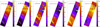 |
Fig. 7 Spatial distribution of the nominal 11.2 µm AIB, its two subcomponents at 11.207 µm and 11.25 µm, and maps of the 11.25/11.207, 11.25/11.2, and 11.207/11.2 ratios. In all maps, contours trace peak emission for the 11.0 µm AIB (white) and the 11.2 µm AIB (teal). The 11.25 µm map includes two sets of black contours at 0.516 10−5 and 1.25 10−5 W m−2 sr−1, which trace the smallest and largest regimes of emission strengths, respectively. The black contour on the 11.25/11.207 map, placed at the level of 0.8, surrounds the region of highest fractional emission. The rest of the map visualization conventions are described in Fig. 4. |
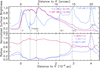 |
Fig. 8 Normalized surface brightnesses and their ratios for the 11.2 µm subcomponents as a function of distance to the IF (0.228 pc or 113.4′′ from θ1 Ori C) along a cut crossing the mosaic (see Fig. 2). Normalization factors are listed in W m−2 sr−1 in parentheses for each surface brightness. As the cut is not perpendicular to the IF and distances are given along the cut, a correction factor of cos(19.58°)=0.942 needs to be applied to obtain a perpendicular distance from the IF. |
5.3.2 Attributes of the 11.2 µm AIB
We investigated the relationships between the extracted components of the 11.2 µm AIB and the nominal 11.0 µm AIB through correlation plots of the measured surface brightnesses of the AIBs. The correlation plot for the 11.0 µm versus 11.2 µm AIB surface brightnesses is presented in Fig. 9 (left panel). As is expected by the spatial behavior of the AIB emission observed in Fig. 4, there exists a strong linear correlation between these two bands, where emission in the 11.0 µm and 11.2 µm AIBs are both the largest in the atomic zone. Yet, there appear to be four disparate trends, which are discussed in detail as follows:
The main trend forms the bulk of the central curved branch, consisting of surface brightnesses originating from DF 2 (orange), the region west of DF 2 (light brown), between DF 2 and DF 1 (yellow), DF 1 (purple), and the atomic PDR (blue), in increasing order of magnitude for both the 11.0 and 11.2 µm AIBs. This trend reflects the general increase in the surface brightnesses of all AIBs toward the PDR surface, since the carrier PAHs are increasingly UV-pumped as the PDR surface is approached.
This main trend exhibits a slightly shallow bend consisting of the 11.0 µm emission arising from PAHs in DF 2 (orange) and the region west of DF 2 (light brown), which then rises steeply as the surface of the PDR is approached.
The lowest end of the 11.0 and 11.2 µm surface brightnesses belong partly to the region beyond DF 3 (light purple), DF 3 itself (pink), the region between DF 2 and DF 3 (brown), and then DF 2 (orange) and the region west of DF 2 (light brown), in increasing order of surface brightnesses. As is seen in the inset in Fig. 9 (left panel), within this region of the lowest end of the (11.2,11.0) surface brightnesses, from the main trend extends a subtly positively linear branch beneath it, which consists of emission primarily from DF 3 (pink), some from the region between DF 2 and DF 3 (brown), and a little from the region beyond DF 3 (light purple). The gentler slope of this branch reflects the additional contribution to the 11.2 µm surface brightness from the 11.25 µm component.
Finally, there is a linear branch of most of the surface brightnesses from the region beyond DF 3 (light purple) extending to meet neighboring spaxels in the atomic PDR (blue). Surface brightnesses from those pixels that are present in the region on the western end below the IF (teal) and that exhibit noticeably lower 11.0 µm surface brightnesses than the rest of the atomic PDR surface brightnesses (blue), also appear to fall on this branch. We further note that surface brightnesses from the H II region bridge this linear relation between the light purple points and the blue points (see Fig. F.1). This shared trend between some of the surface brightnesses from beyond DF 3 (light purple), the H II region, as well as from atomic PDR (blue) and near the IF (teal), if present in all correlations, suggests that the AIB emission in these sight-lines is dominated by the face-on PDR instead of the edge-on PDR. Knight et al. (2022) report that the AIB emission exhibits deviation from solely the edge-on PDR geometry 19′′ beyond the IF, similar to the distance from the IF of the region beyond DF 3 (light purple).
To investigate the origin of these branches in the 11.0 versus 11.2 µm surface brightness relations, we considered correlation plots for the 11.0 µm versus the 11.207 µm and 11.25 µm components (Fig. 9). The 11.0 µm surface brightnesses correlate very strongly with the 11.207 µm surface brightnesses and this pair, along with 11.207 µm and 12.7 µm, exhibits the strongest correlation coefficient in our sample (R = 0.991). The vast majority of data points now lie on a main branch displaying a far stricter positive linear correlation than the 11.0 versus 11.2 µm surface brightnesses. This main trend is now also followed by the spaxels deeper into the molecular cloud, for which we now consider just their 11.207 µm contribution instead of the entire 11.2 µm band’s surface brightnesses. In the atomic PDR, however, there remains noticeable scatter in the (11.0, 11.207) surface brightness values (blue). The deviation toward lower 11.0 µm surface brightnesses at the higher end of 11.207 µm surface brightnesses for species near the IF (teal) remains. Some of the branching trends seen in the correlations of the 11.0 and 11.2 µm surface brightnesses at the lower end, are now no longer seen. However, there remains a displaced, higher branch on which lie the majority of the points beyond DF 3 (light purple) and a few from the atomic PDR (blue) and near the IF (teal).
As is evidenced by the third and fourth panels of Fig. 9, while there exist no relationships at large between the nominal 11.0 µm AIB, or the 11.207 µm component, with the 11.25 µm component of the 11.2 µm AIB, a few prominent features in these plots can shed some light on the nature of the 11.25 µm carriers. We discuss below four differing trends in the 11.0 versus 11.25 µm correlation plot:
At the lowest end of the 11.0 µm surface brightnesses, there is a “flat” branch of points belonging to DF 3 (pink), and a majority of points beyond DF 3 (light purple), for which the 11.25 µm feature varies in brightness between ∼ 0.25–1.6 × 10⁻⁵ W m−2 sr−1. The corresponding 11.0 µm surface brightnesses show very little variation (between 0.75–1.5 × 10⁻⁶ W m−2 sr−1). Some spaxels between DF 2 and DF 3 (brown) belong to this trend, while the rest contribute to the transition to the branch above, which is described below.
Including a few surface brightnesses from beyond DF 3 (light purple) and between DF 3 and DF 2 (brown), the 11.0/11.25 ratios begin to increase toward the middle of DF 2, reflecting a moderate increase in emission at 11.0 µm over a wide range of 11.25 µm surface brightnesses.
Extending from the bottom of DF 2 toward its surface (orange), the 11.25 µm surface brightnesses begin to decrease while the 11.0 µm AIB gets progressively intenser through DF 1 (purple) and into the atomic PDR (blue). This behavior compliments the observations made based on the morphology of the 11.25 µm feature (Sect. 5.3.1), and suggests that the carriers of the 11.25 µm feature are residents of the second and third H2 DFs.
Finally, there appears to be a positively linear trend between some points beyond DF 3 (light purple), atomic PDR (blue) and near the IF (teal), for which both the 11.0 and 11.25 µm surface brightnesses increase, though they are not very strongly linearly correlated.
The contributions of the 11.25 µm component to the 11.2 µm AIB are thus clearly significant. It is also noteworthy that, similar to the correlation plot for the 11.0 and 11.2 µm surface brightnesses, we observe branching behaviors in the correlations of other features with the 11.2 µm AIB (Fig. C.2).
 |
Fig. 9 Correlations plots of the 11.0 µm AIB surface brightnesses versus the 11.2 µm (first panel), 11.207 µm (second panel) and 11.25 µm (third panel) surface brightnesses, and 11.207 µm vs. 11.25 µm (fourth panel) surface brightnesses in units of W m−2 sr−1, on the abscissa and ordinates, respectively. The correlation coefficient “R” for a linear correlation between the variables is displayed in red in the panels. The colored star symbols represent surface brightnesses for the four template spectra from the PDR (atomic PDR: blue; DF 1: purple; DF 2: orange; and DF 3: pink). The inset in the left panel shows a magnified view of the branching occurring at the lower extreme end. Only surface brightnesses with SNR > 3 from every other spaxel are considered. in the correlation analyses. The data points are colored according to regions in the mosaic where those pixels are located (fifth panel). This visual region-color scheme is as follows: blue (atomic PDR), teal (west IF), purple (DF 1), yellow (region between DF 1 and DF 2), orange (DF 2), light brown (region west of DF 2), brown (region between DF 2 and DF 3), pink (DF 3), and light purple (region beyond DF 3). The contours highlighting DF 2 and DF 3 are identified through enhanced emission of H2 0–0 S(3) in these dissociation fronts. The circular red regions on the color-region map (fifth panel) correspond to the proplyds, as these pixels have been masked in our data analysis. |
5.4 The 12.7 µm AIB complex and decomposition
High-resolution Spitzer/IRS maps of the 12.7 µm complex, observed by Shannon et al. (2016), revealed that this band has an asymmetric profile with a broad blue wing. These authors propose a four-component Gaussian model to decompose the 12.7 µm complex. Figure 10 illustrates the complexity of the 12.7 µm profiles, now captured in greater detail by JWST. The 12.7 µm AIB complex is highly asymmetric and comprises a rich terrace-like substructure in its blue wing. Perusing the variability of the profiles in subregions, we find that there are contributions from potentially six components. There appears to be a component in the blue wing between 12.3–12.4 µm. Two components are visible between 12.45–12.7 µm. The 12.7 µm AIB reaches its peak either at ∼12.72 µm or ∼12.78 µm, or peaks doubly in this region between 12.7–12.8 µm. In addition, there appears to be a component within the red wing of the 12.7 µm profile around ∼ 12.95 µm. Based on the examination of these terraces, we propose that the 12.7 µm AIB observed in the Orion Bar comprises at least six components.
Details on the spectral decomposition are given in Appendix A and Fig. 11 displays a few results. Two of the subcomponents of the 12.7 µm complex at 12.55 µm and 12.71 µm in the JWST spectra correspond to the components from Shannon et al. (2016)’s decomposition of Spitzer spectra. While quite effective at large, the present decomposition does not reproduce the double peaks between 12.7–12.8 µm. Moreover, the red wing of the 12.7 µm AIB is not well captured by the 12.7-G6 (12.96 µm) component. The spectral profile near 12.75–12.85 µm may be impacted by the strong Ne line, in particular at closer distances from θ1 Ori C (i.e., the H II region and the atomic PDR), where the Ne line is the strongest. This especially increases the uncertainty of the specific surface brightness of the 12.7 µm AIB over this wavelength range, and thus the surface brightness of the 12.7-G5 (12.805 µm) component.
We present the spatial maps and radial surface brightnesses of the 12.7 µm AIB components in Appendix B and Fig. 12, respectively. The radial surface brightnesses and maps of the relative contributions of the components to the 12.7 µm AIB are shown in Figs. 12 and 13, respectively. We observe that the small contribution from the 12.7-G1 (12.36 µm) component to the overall 12.7 µm AIB emission is consistent across the PDR. The relative contributions of 12.7-G2 (12.55 µm) and 12.7-G3 (12.62 µm) components are large and spatially structured in the atomic PDR. The 12.7-G4 component (12.71 µm) has the largest contribution to the 12.7 µm AIB across the atomic PDR. The surface brightnesses of the last two components 12.7-G5 (12.805 µm) and 12.7-G6 (12.96 µm) relative to the total integrated 12.7 µm AIB, increase beyond DF 1 and are the largest across DF 3. The 12.7-G5 (12.805 µm) component dominates the total 12.7 µm emission in the molecular PDR.
We also investigated the correlations of the 12.7 µm components with the main AIBs, through three-feature intensity ratio correlation plots, which eliminate the effect of differing PAH column densities and PAH abundances. Typically, this normalization is done by using the strongest CHoop band, the 11.2 µm band. However, we have shown that this band encompasses two distinct components (Sect. 5.3). To consider just the PAH contribution to this complex, we thus choose the measured 11.207 µm component as representative of the purely PAH-related 11.2 µm AIB used for normalization. We discuss only the correlations we detect, which are shown in Fig. 14. We find that the most prominent positive linear correlation exists between the Gaussian components centered at 12.805 µm and 12.96 µm, with the higher end of these pairwise surface brightnesses belonging to the molecular zone. Additionally, the 12.805/11.207 and 12.96/11.207 surface brightnesses also strongly anti-correlate with the 11.0/11.207 surface brightnesses.
We observe moderately large positive correlations between the normalized 12.805 µm and 12.96 µm component surface brightnesses and the 13.5 µm and 12.0 µm band surface brightnesses, where the outliers emerge from DF 3 and beyond DF 3. The 12.0, 13.5, 12.805 and 12.96 µm AIBs thus all correlate very well mutually, and similarly anti-correlate with the 11.0 µm AIB, normalized to the 11.207 µm AIB.
In closing, the 12.7 µm AIB observed in the Orion Bar has been decomposed into six subcomponents. The 12.7-G4 component (12.71 µm) has the largest share in the 12.7 µm emission across the atomic PDR, while the 12.7-G5 component (12.805 µm) contributes the most to the total 12.7 µm emission in the molecular PDR. The redder most 12.7 µm subcomponents centered at 12.805 and 12.96 µm correlate well with the 12.0 and 13.5 µm AIBs.
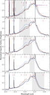 |
Fig. 10 Illustration of the diversity of spectral components of the 12.7 µm AIB complex and their behavior. Profiles are normalized to the peak specific surface brightness between 12.55 µm and 12.8 µm. The short vertical black lines indicate the positions of unresolved lines, with their assignments given in the top panel. The vertical red lines are placed at potential peak wavelengths of the components. Within each panel, the red and blue spectra represent, respectively, the largest and smallest ratios of local peak surface brightnesses of the components that are marked in red in the gray-shaded subregion. We show the same black spectrum, extracted from a single spaxel, in all panels for comparison. |
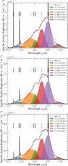 |
Fig. 11 12.7 µm decomposition for three selected spaxels from DF 2 and the atomic PDR. Vertical colored lines indicate the peak positions of the six components (Table A.1). Gaussian fits for narrow lines are shown in gray, and their peak positions are marked by vertical black lines. The percent fractional contribution of the surface brightness carried by each component to the total 12.7 µm surface brightness is indicated in parentheses. |
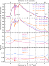 |
Fig. 12 Normalized surface brightnesses and their ratios for the 12.7 µm subcomponents as a function of distance to the IF (0.228 pc or 113.4′′ from θ1 Ori C) along a cut crossing the mosaic (see Fig. 2). Normalization factors are listed in W m−2 sr−1 in parentheses for each surface brightness. |
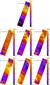 |
Fig. 13 Spatial morphology of the nominal 12.7 µm AIB and of its components, relative to the total integrated 12.7 µm AIB. θ1 Ori C is located toward the top right of each map (see Fig. 2). For each map, the range of the corresponding color bar is set between 0.5% and 99.5% percentile level for the data, while zero pixels, edge pixels, and pixels covering the two proplyds, indicated by the black circles, are masked out. The contours trace peak emission for the 11.0 µm AIB (white), the 11.2 µm AIB (teal). The rectangular apertures of the template spectra for the H II region, atomic PDR, DF 1, DF 2 and DF 3, from top to bottom, are shown in white and the solid white lines delineate the IF and the three dissociation fronts, DF 1, DF 2 and DF 3. |
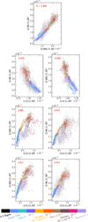 |
Fig. 14 Correlation plots for the 12.805 µm and 12.96 µm components of the 12.7 µm AIB. The red text displays the value of the correlation coefficient “R” for the data points plotted. The data points are colored according to regions in the mosaic where those pixels are located, per the color bar at the bottom and the map in Fig. 9. |
5.5 Insights into the 12.0 µm AIB
The observed increase in the 12.0 µm AIB emission at DF 2 and DF 3 (Fig. 5) prompts a closer look at the 12.0 µm AIB profiles. These profiles do indeed display spectral variability across the Orion Bar (Fig. 15)9. In this section we present two decompositions of the 12.0 µm AIB: a traditional Gaussian mixture model and a decomposition based on fitting the 11.207 µm and 11.25 µm spectral maps, in Sects. 5.5.1 and 5.5.2, respectively.
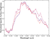 |
Fig. 15 Illustration of the spectral diversity of the 12.0 µm profile in the Orion Bar. Spectra from consecutive pixels were averaged and three of these averaged, normalized profiles are presented. |
5.5.1 The 12.0 µm AIB Gaussian decomposition
We decompose the 12.0 µm AIB into six components, adopting the same methodology as for the 12.7 µm AIB, where the fit parameters are given in Table A.1. This decomposition successfully reproduces the spectral complexity of this weak AIB (Fig. 16). We note, however, that this model underestimates the specific surface brightnesses around ∼ 12.05 µm in the atomic PDR spectra.
We present the morphology of these 12.0 µm subcomponents in Fig. B.2, their morphology relative to the 12.0 µm surface brightnesses in Fig. 17, and their behavior as a function of distance from the IF in Fig. 18. All components exhibit similar behavior, with their surface brightnesses declining across the atomic PDR and increasing at the DFs. However, the 12.0-G1 (11.90 µm) component emerges as the dominant contributor to the 12.0 µm AIB within the DFs, while the largest contribution to the 12.0 µm AIB in the atomic PDR originates from the 12.0-G4 (12.01 µm) component (Fig. 18).
The 12.0 µm subcomponents are found to have very strong linear correlations (R > 0.9) among each other. We present the most notable correlations in Fig. 19, where we also highlight the very tight correlation of the 12.0 µm AIB with the 11.25 µm AIB. Among the six 12.0 µm subcomponents, 12.0-G2 (11.95 µm) exhibits the strongest linear correlation with 11.25 µm AIB.
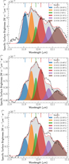 |
Fig. 16 12.0 µm decomposition for three selected spaxels from DF 2, the middle of the atomic PDR and near the IF. The vertical colored lines indicate the central positions of the six components (Table A.1). The percent fractional contribution of the specific surface brightness carried by each component to the total 12.0 µm surface brightness is indicated in parentheses. |
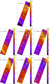 |
Fig. 17 Morphology of the 12.0 µm AIB surface brightness and its components relative to the total integrated 12.0 µm AIB. The white and teal contours trace peak emission for the 11.0 and 11.2 µm AIBs, respectively. The map visualization conventions are described in Fig. 13. Near proplyd 1, the decomposition was unsuccessful, hence the lack of data. |
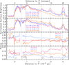 |
Fig. 18 Normalized surface brightnesses and their ratios for the 12.0 µm components as a function of distance to the IF (0.228 pc or 113.4′′ from θ1 Ori C) along a cut crossing the mosaic (see Fig. 2). Normalization factors are listed in W m−2 sr−1 in parentheses for each surface brightness. |
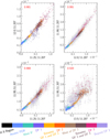 |
Fig. 19 Noteworthy correlations for the 12.0 µm AIB and its components. The red text displays the value of the correlation coefficient, R, for the data points plotted. The data points are colored according to regions in the mosaic where those pixels are located, per the color bar at the bottom. |
5.5.2 The 12.0 µm AIB decomposition with 11.207 and 11.25 µm maps
Motivated by the remarkably positive correlations between the 12.0 µm AIB and its components with the 11.25 µm AIB (Fig. 19), we performed a second decomposition of the 12.0 µm profiles utilizing the 11.207 µm and 11.25 µm maps as follows:
We fit the surface brightness map at each wavelength λ within the domain for the 12.0 µm AIB, using a linear combination of the 11.207 and 11.25 µm surface brightness maps:
![Mathematical equation: \[{I_{\lambda \in [11.8,12.2]}} = {a_\lambda }{I_{11.207}} + {b_\lambda }{I_{11.25}}.\]](/articles/aa/full_html/2025/07/aa54096-25/aa54096-25-eq3.png)
-
For each spaxel i, we reconstructed the 12.0 µm profile, over the spectral region (λ ∈ [11.8, 12.2]) such that the specific surface brightness at each wavelength (F12.0,i,λ) is
![Mathematical equation: \[\begin{array}{*{20}{c}}{{F_{12.0,i,\lambda }} = {a_\lambda }{I_{11.207,i}} + {b_\lambda }{I_{11.25,i}}}\\{\,\,\,\,\,\,\,\,\, = {{12.0}_{1,i,\lambda }} + {{12.0}_{2,i,\lambda }},}\end{array}\]](/articles/aa/full_html/2025/07/aa54096-25/aa54096-25-eq4.png)
where 12.01,i and 12.02,i refer to the profiles contributing to the 12.0 µm spectral profile of spaxel i using the fit 11.207 and 11.25 µm surface brightnesses, respectively.
A weighted average of all the 12.01,i and 12.02,i profiles was performed, producing two distinct component profiles (Fig. 20). “Component 1” is hereafter labeled as 12.01 and “component 2” as 12.02.
Similar to the decomposition of the 11.2 µm AIB, we performed a linear combination of these two 12.0 µm component profiles to fit the 12.0 µm profile at each spaxel.
Surface brightness maps,
 and
and  for the two 12.0 µm AIB components were obtained by integrating the specific surface brightnesses of the two weighted component profiles for each spaxel.
We obtained excellent fits, as is illustrated in Fig. 20. The spatial distributions of the 12.0 µm AIB and these two components are displayed in Fig. 21. This decomposition clearly distinguishes the two independent components contributing to the 12.0 µm AIB. Component 12.01 behaves spatially akin to the AIBs tracing PAH emission in the Orion Bar (Figs. 4 and 22). On the other hand, the morphology of the 12.02 component is recognizably distinct: the 12.02 component is weak in the atomic PDR, and grows progressively stronger across the DFs, exhibiting a strikingly similar behavior to that of the 11.25 µm AIB (Figs. 21 and 22). Additionally, as seen in the 11.25 µm AIB morphology (Fig. 7), an enhanced 12.02 surface brightness is observed in the close vicinity of the IF (Fig. 21). We further observe that the 12.01 component contributes to the 12.0 µm AIB in the atomic PDR, while 12.02 is the main contributor to the 12.0 µm AIB beyond DF 1. Comparing these two 12.01 and 12.02 components with the six Gaussian components, we find all the six Gaussian components to correlate strongly with just the 12.02 component (illustrated for 12.0-G1 (11.90 µm) component in Fig. 23). This analysis demonstrates that the second decomposition is highly effective at revealing two independent contributors to the 12.0 µm AIB, whereas the first decomposition, based solely on spectral components, does not achieve this distinction. While the second decomposition employs the spatial morphology of the 11.207 µm and 11.25 µm AIBs as input, we only achieve excellent fits when applied to the 12.0 µm AIB, but not when applied to the 12.7 µm AIB. This strengthens the observation that the 12.0 µm AIB has a subcomponent that has a spatial distribution akin to that of the 11.25 µm AIB.
In summary, to investigate the spectral diversity of the 12.0 µm AIB observed in the Orion Bar, two different decomposition methods were adopted. Akin to the 12.7 µm AIB, we introduce a six-component Gaussian decomposition of the 12.0 µm AIB. Prompted by the strong correlations of the 12.0 µm AIB and its subcomponents with the anomalous 11.25 µm component, we also decompose the 12.0 µm AIB into two components, utilizing the 11.207 µm and 11.25 µm maps (Sect. 5.3.1). This decomposition positively affirms that analogous to the 11.2 µm AIB, the 12.0 µm AIB comprises two spectroscopically distinct components that have distinct spatial distributions.
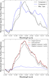 |
Fig. 20 Top: Normalized 12.0 µm spectral profile from a spaxel in the atomic PDR, and the two components used in the 12.0 µm decomposition, based on fitting the 11.207 µm and 11.25 µm maps. Bottom: Linear combination fitting of a 12.0 µm profile by these two components shown in the top panel. |
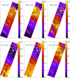 |
Fig. 21 Spatial distribution of the 12.0 µm AIB, its two subcomponents and 12.02 (second decomposition), and their ratios. The 12.02 µm map includes a set of black contours at 1.15 × 10⁻⁶ W m−2 sr−1, and blue contours trace the peak 11.25 µm emission at 1.25 × 10⁻⁵ W m−2 sr−1. θ1 Ori C is located toward the top right of each map (see Fig. 2). For each map, the range of the corresponding color bar is set between 0.5% and 99.5% percentile level for the data, while zero pixels, edge pixels, and pixels covering the two proplyds, indicated by the black circles, are masked out. The contours trace peak emission for the 11.0 µm AIB (white), the 11.2 µm AIB (teal). The rectangular apertures of the template spectra for the H II region, atomic PDR, DF 1, DF 2 and DF 3, from top to bottom, are shown in white and the solid white lines delineate the IF and the three dissociation fronts, DF 1, DF 2 and DF 3. |
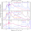 |
Fig. 22 Normalized surface brightnesses and their ratios for the 12.0 µm subcomponents and the 11.207 and 11.25 µm surface brightnesses, as a function of distance to the IF (0.228 pc or 113.4′′ from θ1 Ori C) along a cut crossing the mosaic (see Fig. 2). Normalization factors are listed in W m−2 sr−1 in parentheses for each surface brightness. As the cut is not perpendicular to the IF and distances are given along the cut, a correction factor of cos(19.58°)=0.942 needs to be applied to obtain a perpendicular distance from the IF. |
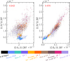 |
Fig. 23 Correlations of the 12.0-G1 (11.90 µm) subcomponent with the 12.01 and 12.02 components. The red text displays the value of the correlation coefficient, R, for the data points plotted. The data points are colored according to regions in the mosaic where those pixels are located, per the color bar at the bottom. |
5.6 Spectral diversity of the 13.5 µm AIB
Prompted by the enhanced 13.5 µm AIB emission across DF 2 and DF 3 (Fig. 5), similar to the 12.0 µm and 11.2 µm AIBs, we inspect the spectral variability in the 13.5 µm AIB profiles (Fig. 24). Secondary and tertiary components, albeit weak, emerge at ∼13.2 µm and ∼ 13.65 µm in DF 3, in addition to the primary contributor responsible for the AIB’s peak between ∼13.55–13.58 µm. These components are most likely responsible for the noticeable enhancement in the overall 13.5 µm AIB surface brightnesses at DF 3. Due to the weakness of this band, we are unable to devise a suitable decomposition methodology to isolate its potentially independent components.
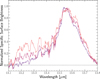 |
Fig. 24 Profile variations in the 13.5 µm AIB, in the Orion bar. Spectra from consecutive pixels were averaged and three of these averaged profiles are presented. Deeper into the molecular cloud, toward the DF 3 (orange spectrum), additional components emerge around ∼13.2 µm and ∼13.55 µm. |
5.7 Notable correlations in relative strengths of the 10–15 µm AIBs
Pairwise correlations in absolute surface brightnesses of the 10.6, 10.8, 11.0, 11.2, 12.0, 12.7, 13.5, 14.0, and 14.2 µm AIBs and the subcomponents of the 11.2, 12.0 and 12.7 µm AIBs, reveal that correlations, strong and weaker ones, exist between all the AIBs (see Fig. C.2 for correlations with the 11.2 µm AIB and Appendix C). This is driven by the general trend for the typical AIB emission; that is, the strongest emission occurs in the atomic PDR, and then declines deeper into the PDR beyond either DF 1 or DF 2 (Figs. 4 and 5). As the AIBs are attributed to emission from PAHs and their intensity is governed by PAH abundance and excitation, this general decrease reflects the increasing attenuation of FUV photons by dust with depth into the PDR and results in correlations between all AIBs. The tightness of the correlation then indicates variations within the PAH population and hence the relative AIB surface brightnesses, in the different regions of the PDR.
In this section, we present the salient correlations detected between the relative strengths of the 10–15 µm AIBs. The largest three-feature intensity ratio correlations with |R| > 0.8 involve the 13.5, 12.0, and 14.2 µm AIBs and the 11.0 µm AIB. Indeed, the 13.5 µm AIB anti-correlates very well with the ionic 11.0 µm AIB, when normalized to the 11.207 µm surface brightnesses (Fig. 25). These pairwise ratios originating from the atomic zone are situated at the upper limit of the 11.0/11.207 µm surface brightness ratios, and the lower limit of the 13.5/11.207 µm ratios. These ratios experience a bend, as the 13.5/11.207 surface brightnesses increase from the atomic PDR (blue) toward DF 1 (purple) and DF 2 (orange). Chown et al. (2024) and Schefter et al. (in prep.) infer the presence of smaller-sized PAHs in DF 1 than the atomic PDR. As a result, the 11.2 µm profiles have larger FWHMs in the molecular PDR. However, we do not consider changes in FWHMs for the two components used in our decomposition of the 11.2 µm AIB (Sect. 5.3.1) and may thus be underestimating the 11.207 µm surface brightnesses. This bend may thus be explained by the overestimation of the 11.0/11.207 µm surface brightnesses beyond DF 1.
An analogous trend is observed for the normalized 12.0 µm surface brightnesses compared to the 11.0 µm surface brightnesses, albeit with a larger bend in the main, tight trend. As is seen in Sects. 5.2 and 5.5, the 12.0 µm AIB emission is much more enhanced in DFs 2 and 3, compared to the increase in strength for the 13.5 µm AIB at these DFs. This sharper bend for the 12.0/11.207 and 11.0/11.207 µm surface brightnesses beyond DF 1 can thus be due to the larger 12.0 µm surface brightnesses in DF 2 and DF 3, along with the influence of the overestimated 11.0/11.207 surface brightnesses. At large, the spatial emission of the 12.0 and 13.5 µm AIBs exhibit similarities as discussed in Sect. 5.2. As seen in Fig. 25 they also positively linearly correlate in normalized surface brightnesses, where once again, the surface brightnesses arising in DF 3 (pink) and the region beyond (light purple) deviate from the linear trend. The 12.0 µm and 13.5 µm AIBs are clearly related. The 13.5 µm AIB also exhibits a strong positive linear relationship with the 11.25 µm AIB surface brightnesses; however, it is less tight than the 12.0 versus 11.25 µm correlation (Fig. 19).
Furthermore, we also observe a positive linear relationship between the 14.2 µm AIB and the 11.0 µm AIB within the atomic PDR. There also exists a moderately strong anti-correlation (R = –0.864) between the normalized 14.2 and 12.0 µm AIBs.
Perusal of the heat maps in Fig. C.1 and all three-feature correlation plots lends weight to the following conclusions:
The absolute surface brightnesses of all the AIBs in the collection under study correlate strongly with each other; that is, |R| ≥ 0.8. These bands are all accredited to emission at mid-IR wavelengths from vibrationally excited PAHs.
The weak band at 10.6 µm correlates well with the 10.8 µm −0.25 0.00 0.25 0.50 PC1 band, when normalized to the 11.207 µm band (R = 0.783).
The 11.0 µm AIB anti-correlates most strongly with the 13.5 µm AIB followed by 12.0 µm, whereas the normalized surface brightnesses of the 11.0 µm and 14.2 µm AIBs positively correlate.
The 12.0 µm AIB correlates very strongly with the 13.5 µm AIB, and negatively with the 11.0 µm and 14.2 µm AIBs. The 12.0 µm AIB has enhanced emission in the DFs, which is greater than that of the 13.5 µm AIB. The 12.0 µm AIB and its six spectral subcomponents positively linearly correlate with the anomalous 11.25 µm AIB.
In addition to positively correlating with the 12.0 µm AIB, the 13.5 µm AIB also correlates negatively with the 11.0 µm AIB. The 13.5 µm AIB correlates with the 11.25 µm AIB, albeit with large variability in regions beyond DF 2.
The poorest correlations belong to the pairs of normalized surface brightnesses involving the 14.0 µm AIB. The 14.2 µm AIB in comparison, has a strong negative correlation with the 12.0 µm AIB, and a positive correlation with the 11.0 µm AIB.
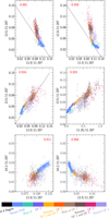 |
Fig. 25 Correlation plots for the 13.5, 12.0, and 14.2 µm bands normalized to the 11.207 µm AIB. The red text displays the value of the correlation coefficient, R, for the data points plotted. The dotted black lines in the first three panels, represent either a positive or negative linear relationship between a set of two variables. The data points are colored according to regions in the mosaic where those pixels are located, per the color bar at the bottom. |
5.8 Principal component analyses of the 10–15 µm AIBs
In addition to the analysis based on spatial morphologies and correlations, we also adopted a statistical approach to analyze the variations in the AIB emission. We performed several principal component analyses (PCA) of the entire cohort of AIBs at 10.6, 10.8, 11.0, 11.2, 12.0, 12.7, 13.5, 14.0, and 14.2 µm, and the decomposed components of the 11.2, 12.0, and 12.7 µm AIB complexes by varying the input AIBs. The details of the mathematical formalism and the input and results of these PCA rounds are provided in Appendix D. In this section, we discuss only the prominent results of the PCA analysis that involves the 11.2, 12.0, and 12.7 µm decompositions, and the remainder of the AIBs (referred to as round 3 in Appendix D). We emphasize that these results are based on the second (spectral map-fitting) decomposition considered for the 12.0 µm AIB (see Sect. 5.5.2), as it provides more pronounced and informative results, whereas the Gaussian decomposition is significantly less informative.
Our multivariate data comprising surface brightnesses of various AIBs and their decomposed components can be represented by two independent, principal components, PC1 and PC2. These principal components are linear combinations of the standardized surface brightness variables (zAIB), which are supplied as inputs for the PCA. We find that PC1 and PC2 together explain ∼ 97.08% of variance in the data. Based on their spatial morphologies, PC1 and PC2 trace two populations of carriers responsible for the broad mid-IR 10–15 µm spectral features (Fig. 26).
We observe differing behavior in the projections of the standardized surface brightness variables onto the axes defined by PC1 and PC2 (Fig. 27). In particular, z11.25 and  have the largest projections on the PC2 axis, and minimal PC1 projections. With the exception of these two components, the surface brightnesses of the other AIBs correlate strongly with PC1. These projections, along with correlations with the total and individual AIB surface brightnesses, provide valuable clues about the physical interpretations of the principal components.
As is evident in Fig. 28, PC1 exhibits a strong positive linear correlation with the total surface brightness; that is, the sum of all the surface brightnesses considered for the PCA. However, this correlation becomes tighter and almost linear (R = 0.998) when the 11.25 µm and 12.02 surface brightnesses are omitted. Of all individual bands, PC1 correlates most strongly with the surface brightnesses of the 11.207 µm AIB, characteristic of PAH fluorescence. Thus, in this analysis, PC1 represents the total PAH emission in the 10–15 µm regime.
In contrast, PC2 correlates only with the 11.25 µm and 12.02 surface brightnesses (Fig. 28). Two “branches” for surface brightnesses within the atomic PDR and near the IF, and surface brightnesses from the molecular PDR are clearly visible in the 11.25 µm-PC2 correlation plot. The widths of the components used to fit the 11.2 µm spectral profiles are kept constant throughout the mosaic (Sect. 5.3.1), such that the surface brightnesses of the 11.207 µm and 11.25 µm bands may be underestimated and overestimated, respectively, in the molecular PDR. We therefore propose that the origin of this branching behavior observed in the 11.25 µm–PC2 correlation plot is due to the overestimation of the 11.25 µm AIB surface brightnesses in the molecular PDR. A similar branching behavior is also seen in the 12.02–PC2 correlation plot, for the same reason since the 11.25 µm map was used to measure the 12.02 component (Sect. 5.5.2). A semblance of a linear correlation between PC2 and the surface brightnesses of the 13.5 µm AIB appears in the molecular PDR. Based on the tight PC2, 11.25 µm and 12.02 µm surface brightness correlations, and the distinctly different spatial behavior of the 11.25 µm and 12.02 components from the other principal AIBs, we conclude that PC2 in this PCA analysis, traces spectral emission which is independent of the PAH emission typical for the Orion Bar, in the 10–15 µm regime.
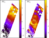 |
Fig. 26 Spatial maps of the first two principal components (PC1 and PC2) derived from a PCA of the various 10–15 µm AIBs and their sub-components. Only surface brightnesses with SNR >3 and originating in the PDR (i.e., excluding the H II region) are considered for the analysis. |
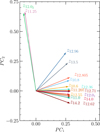 |
Fig. 27 Biplot illustrating the contributions of the AIBs and their sub-components to the principal components, PC1 and PC2. |
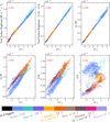 |
Fig. 28 Top panel: Correlations of PC1 with the total surface brightness i.e., the sum of the surface brightnesses of all the AIBs (left), with the total surface brightness without contributions from the 11.25 µm and µm components (middle), and the 11.207 µm AIB surface brightnesses (right). Middle panel: From left to right, correlations of PC2 with the 11.25 µm, 12.02 µm and 13.5 µm AIB surface brightnesses. Bottom panel: The data points are colored according to regions in the mosaic where those pixels are located, per the color bar. |
6 Discussion
An extensive analysis of the broad AIBs in the 10–15 µm wavelength range of the Orion Bar PDR reveals their origin in vibrational relaxation of excited PAHs. Spatial-spectral maps of the surface brightnesses of these AIBs reveal the shared and unique morphologies of emission in these bands and trace the large-scale structure of the PDR. As also observed for the AIB components in the 3.2–3.7 µm range, revealed through JWST NIRSpec IFU spectroscopy (Peeters et al. 2024), the highly structured PAH 10–15 µm emission in the atomic zone of the PDR, elucidates the complexity of the geometry and small-scale structures in the Orion Bar. Moreover, analyses of the spatial morphologies and correlations of the astronomical AIBs in this cohort, as well as employing the statistical technique of PCA yield new and intriguing insights into the nature of these spectral features and in particular, the edge structures of their molecular carriers.
We discuss the spectroscopic assignments of the observed AIBs and their subcomponents in Sect. 6.1. The inferred molecular structures of the PAHs in the Orion Bar are discussed in Sect. 6.2. Lastly, we discuss the evidence for a population of VSGs in the Orion Bar in Sect. 6.3.
6.1 Assignments of the 10–15 µm CH out-of-plane bands in PAHs
The PAH 10–15 µm features arise from out-of-plane bending of peripheral solo, duo, trio, quartet, or quintet hydrogen groups, in neutral and charged species. We discuss existing hydrogen-adjacency class and charge state assignments of these bands that have been proposed in literature, and new insights from the highest-quality astronomical observations of the Orion Bar to date. Figure 29 presents this assortment of assignments for the AIBs studied.
Spectroscopic studies of PAHs strongly establish that the weak AIB at 11.0 µm arises from out-of-plane vibrations of solo CH bonds in positively charged PAHs, while the traditional, strong 11.2 µm interstellar band is widely considered to arise from solo CH groups in neutral PAHs (Hudgins & Allamandola 1999; Hony et al. 2001; Bauschlicher et al. 2008, 2009; Rosenberg et al. 2011). In the following interpretations, we thus take the PAH 11.0 µm AIB to be the canonical (cat)ionic AIB, and consider the 11.207 µm AIB to arise from neutral PAHs with both bands due to solo CH-groups. We ascribe the 11.25 µm AIB to VSGs or the solo CHoop mode in PAH clusters. This assignment is discussed in Sect. 6.3.
We discuss the vibrational mode assignments for the 12.0 µm and 12.7 µm AIBs and their subcomponents as follows. Based on studies of observational data and laboratory results by Hony et al. (2001) and of theoretical results by Bauschlicher et al. (2009), about half of the 12.7 µm AIB intensity can be attributed to trio hydrogens. Furthermore, the weak interstellar 12.0 µm AIB arises from out-of-plane vibrations of duo hydrogens in PAHs (Hony et al. 2001). Computed spectra based on density functional theory by Bauschlicher et al. (2008) further reveal that coupling between the solo and duo CHoop modes in PAHs that have only solo and duo hydrogens, splits the duo CHoop mode into two. In large, compact, symmetric PAHs, this split results in a “duo1” mode within ∼ 11.5–12.0 µm that is slightly stronger than the “duo2” mode falling between ∼ 12.5–13.2 µm (Bauschlicher et al. 2008). In large, irregular PAHs, the weak duo1 band lies between 11.3 – 12.3 µm, and the stronger duo2 band falls between ∼ 12.3–12.8 µm (Bauschlicher et al. 2009). Thus, the longer wavelength duo2 mode falls in the region traditionally assigned to the trio CHoop mode. Based on the second decomposition of the 12.0 µm AIB (Sect. 5.5.2), we posit that the 12.01 component is representative of the duo1 mode in PAHs. In contrast, 12.02 is carried by VSGs (see Sect. 6.3). In terms of the classification of the six spectral components of the 12.0 µm AIB identified through the first decomposition (Sect. 5.5.1), we conclude that the components are amalgamations of PAH duo1 CHoop modes and vibrational modes in VSGs and/or PAH clusters. The variations in the relative surface brightnesses of the components with increasing distances from the PDR surface (Figs. 17 and 18) show that 12.0-G1 (11.90 µm) component dominates the 12.0 µm AIB at the DFs, in a pattern resembling that of the 11.25/11.2 surface brightness ratio (Fig. 8). This short wavelength component of the 12.0 µm AIB is assigned to VSGs (see Sect. 6.3).
The 12.7 µm AIB complex comprises both duo and trio CHoop modes in PAHs. Comparing the representative band strengths for the trio, duo2, and duo1 modes in compact and irregular PAHs presented by Bauschlicher et al. (2009), we assert that if the duo1 mode arises from compact PAHs, the duo2 mode contributes only marginally to the 12.7 µm complex, and would be the 12.96 µm component, while the other components arise due to the trio CHoop mode. In irregular PAHs, the duo2 mode is strong. Comparing the surface brightnesses of the 12.7 µm components with the 12.01 component, we assign the 12.55 µm and 12.62 µm components to the duo2 mode in irregular PAHs, while the 12.36 µm, 12.71 µm and 12.805 µm components would be the trio CHoop modes. Further, the 12.7 µm AIB and its components lack strong correlations with the ionic 11.0 µm AIB. Meanwhile, only the two components at 12.805 µm and 12.96 µm exhibit strong, positive correlations with the 11.207 µm (Fig. C.3). We note that while studies of reflection nebulae NGC 7023 and NGC 2023 by Shannon et al. (2016) reveal clear cationic and neutral contributions to the 12.7 µm complex, we do not see evidence of any dominating components which distinctly trace the neutral and cationic PAHs in the Orion Bar. The peak 11.0 and 11.2 µm spatial emissions are well separated in these reflection nebulae, revealing the spatially displaced populations of the ionic and neutral PAHs. In contrast, the 11.0 and 11.2 µm PAH peak emission both occur in the atomic PDR in the Orion Bar. Thus owing to its geometry, it is difficult to disentangle the charged and neutral contributions to the 12.7 µm AIB complex in the Orion Bar. Moreover, theoretically calculated intrinsic PAH spectra exhibit similar intrinsic strengths for the cations and neutrals CHoop modes (e.g., Bauschlicher et al. 2009; Ricca et al. 2012). Combined with the observed relative strength of the 11.0 and 11.2 µm AIBs in the Orion Bar, this suggests that the cationic duo and trio CHoop modes may be similarly weak as the cationic solo CHoop mode. In that case, the contributions of cations to the 12.7 µm AIB observed in the Orion Bar, are to be minimal.
The cases of the other AIBs studied are discussed as follows. The 10.6 µm AIB has been observed in a variety of astronomical sources, including H II regions, young stellar objects, and evolved stars (Hony et al. 2001). Hony et al. (2001) attribute the 10.6 µm AIB to solo modes in cationic PAHs based on matrix isolated spectroscopy of neutral and cationic PAHs and quantum chemical calculations by Hudgins & Allamandola (1999). In their study of theoretically computed IR spectra of large, irregular PAHs, Bauschlicher et al. (2009) particularly note that the bands at 9.5, 10.2, and 10.6 µm in C120H36, one of the six molecules studied, are all related to C-C stretching vibrations and deformations of the benzene rings containing quartet hydrogens. Per Fig. C.1, we find that the absolute surface brightnesses of the 10.6 µm AIB correlate strongly with the other AIBs, but rather poorly when normalized to the 11.207 µm surface brightnesses. Thus, we propose that the 10.6 µm AIB most likely emerges not due to CHoop modes of solo CH groups in PAHs, but by another mechanism such as the above one proposed by Bauschlicher et al. (2009). In the case of the 10.8 µm AIB, its normalized surface brightnesses correlate moderately with the normalized surface brightnesses of 12.0 and 13.5 µm AIBs. Bauschlicher et al. (2009) found that for the PAHs in their study, the CHoop band for the solo hydrogens falls between 10.983 and 11.206 µm for the cations. The 10.8 µm band anti-correlates rather weakly with the 11.0 µm AIB (R = –0.668, per Fig. C.1). A cationic origin of the 10.8 µm AIB would result in a strong positive correlation with the 11.0 µm AIB, which is absent in our observations. Like its bluer counterpart at 10.6 µm, we propose that the 10.8 µm AIB likely originates from a vibrational mode in PAHs other than an CHoop mode or due to an anharmonic coupling between CHoop modes.
The 13.5 µm AIB surface brightnesses correlate very well with the 12.0 µm AIB surface brightnesses, and they anticorrelate with the 11.0 µm AIB (R = –0.881, per Fig. C.1). Based on the spectral diversity of the 13.5 µm AIB (Sect. 5.6), it is possible that this band has a weak VSGs and/or PAH cluster component, which could not be identified in this work, as has been done for the 11.2 µm and 12.0 µm AIBs. However, the predominant emission in the 13.5 µm AIB as observed in the Orion Bar, originates from out-of-plane bending of quartets due to pendant rings on PAH molecules (Hudgins & Allamandola 1999; Hony et al. 2001; Bakker et al. 2011).
The weak 14.0 µm AIB does not correlate with any of the other AIBs in this cohort, when three-feature intensity ratios are considered (see Fig. C.1). However, the absolute surface brightnesses of this AIB do indeed correlate well with the other 10–15 µm AIBs. We propose that the 14.0 µm AIB may be due to a mechanism other than CHoop bending in PAHs. The adjacent, stronger 14.2 µm AIB may arise due to quintet hydrogens (Hony et al. 2001). However, quintet hydrogen groups are inherently unstable structures. Alternatively, a weak CCC bending mode appears in the 14–14.5 µm range, due to trio and quintet hydrogens (Hony et al. 2001). Based on its strongest positive correlation with the ionic 11.0 µm AIB, when normalized (R = 0.811), the carrier of the 14.2 µm AIB has been designated as cationic. A cationic nature implies that the carriers reside in environments exposed to strong UV radiation fields (e.g., the atomic PDR), where the quintets are more susceptible to photo-destruction. Thus, it is unlikely that the band arises from vibrational modes involving fragile quintet hydrogens. We further note that, unlike the cationic 11.0 µm AIB, which has a stronger neutral counterpart at 11.2 µm, the 14.2 µm AIB lacks such a corresponding neutral counterpart.
The PCA discussed in Sect. 5.8, and the positive correlations of these 10–15 µm AIBs and subcomponents with the PAH-emission-tracing PC1, corroborate the above conclusions about the origins of these AIBs in IR florescence of PAHs, either as CHoop modes or other vibrational modes in this class of molecules. However, we emphasize that the picture presented in Fig. 29 and discussed above is an oversimplification as couplings between solo, duo, trio, and quartet hydrogens shift the band positions. Nonetheless, out-of-plane bending of a particular CH-group would dominate the vibrational mode. We further note that these assignments are based on harmonic calculations with a limited basis set, but the 10–20 µm spectral region is not much affected by anharmonicity and resonances (Mackie et al. 2022). We note that experimental studies of the IR spectra of PAHs have been used to support the theoretical link between PAH molecular structure and the CHoop frequencies (e.g., Hudgins & Allamandola 1999; Bakker et al. 2011; Lemmens et al. 2021). In addition, even though the CHoop modes dominate the 10–15 µm region, other modes such as skeletal, C–C–C, and C–C ring deformation modes can appear within this region (e.g., Califano 1962; Langhoff 1996; Candian et al. 2014). Likewise, the influence of hydrogenation of PAHs is not considered. Detailed investigations of a large variety of PAHs through experimental and theoretical approaches are required in developing nuanced assignments of these AIBs, including the myriad subcomponents identified within the 12.0, 12.7 µm and 13.5 µm band complexes.
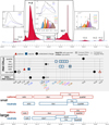 |
Fig. 29 Qualitative representation of the assignments for the 10–15 µm AIBs and subcomponents. Top panel: Typical spectrum from the Orion Bar showcasing the AIBs. The insets show the decompositions for the 11.2, 12.0, and 12.7 µm AIBs. Middle panel: Proposed charge (color) and vibrational mode (marker) assignments of the 10–15 µm AIBs in terms of their carriers – PAHs or VSGs and/or PAH clusters, and vibrational modes. The “duo1” and “duo2” modes refer to the two modes that the duo CHoop mode splits into in PAHs with only solo and duo hydrogens (Bauschlicher et al. 2008, 2009). Bottom panel: Boxes representing the theoretical ranges of CHoop modes for small and large, cationic and neutral PAHs. The ranges for small (≲50 carbon atoms) cations and neutral PAHs are taken from Hony et al. (2001). The ranges for large (50–130 carbon atoms) neutral PAHs are derived from Bauschlicher et al. (2009, which is based on based on a small sample of PAHs), while those for their cationic counterparts are obtained from the NASA Ames PAH IR Spectroscopic Database (PAHdb) (Bauschlicher et al. 2010; Boersma et al. 2014; Bauschlicher et al. 2018). No redshift has been applied for these wavelength ranges. See text for details. |
6.2 Molecular structures of PAHs in the Orion Bar
Aided by the assignments of the AIBs in the CHoop region to the number of peripheral CH groups, we are now able to characterize the molecular structures of PAHs in the Orion Bar, using the relative observed and intrinsic strengths of these bands. Based on the computed spectra of large, neutral PAHs, Bauschlicher et al. (2009) present the representative hydrogen adjacency class band strengths [km/mol−1] that are tabulated in Table 1. We note that the intrinsic properties taken from Bauschlicher et al. (2009) are based on a collection of 15 PAHs.
Per Sect. 6.1, we assume that the 11.207, 12.01, and 13.5 µm AIBs arise due to solo, duo1, and quartet hydrogens, respectively. As seen in Table 1, while the duo1 and duo2 modes both originate from peripheral duo CH groups in the same PAH molecules, the ratio of their intrinsic strengths – duo2/duo1 – is 1.25. Since observationally the duo1 mode is reflected by the emission in the 12.01 band, and the 12.7 µm emission band comprises the duo2 and trio CHoop modes, we take the observed strength of the band due to only trio hydrogens to be the difference of the 12.7 µm band surface brightnesses and the 12.01 band surface brightnesses weighted by this factor of 1.25. We are thus able to derive the relative number of hydrogen atoms in each class in regions across the Orion Bar, by using the ratios of the intrinsic CHoop band strengths in Table 1 and the observed surface brightnesses of the resulting AIBs. Finally, accounting for the number of hydrogen atoms in each class, we derive the number of the edge CH groups in PAHs, which produce the corresponding 10–15 µm AIBs emission in the Orion Bar, which are presented in Table 2. For comparison, Table 2 includes the values for the PAHs in the H II region IRAS 18317-0757 and the planetary nebula NGC 7027, determined by Hony et al. (2001). Based on the large s/d and s/q ratios, Hony et al. (2001) concluded that the PAH family in NGC 7027 is dominated by large compact PAHs with long, straight edges, whereas the extreme solo-to-quartet group ratio necessitates an absence of quartet groups in PAHs. While the inferred ratios of various CH groups in PAHs in the Orion Bar do not match exclusively with either of these other targets, the large solo-to-duo and solo-to-quartet ratios are large, and decrease from the PDR surface to the H2 dissociation fronts. It is difficult for a single molecule or two molecules to encapsulate the various number of relative groups reflected by the ratios presented in Table 2. The extreme s/q ratios further imply that quartet groups are absent in the vast majority of the molecules in the Orion Bar, and while still scarce, are more prevalent in DF 3 than in atomic PDR. We present a few structures that exemplify the derived s/t and s/q CH group ratios, for the atomic PDR and DF 3, in Fig. 30. A detailed comparison with the NASA Ames PAH IR spectral database (PAHdb: Bauschlicher et al. 2010; Boersma et al. 2014; Bauschlicher et al. 2018; Maragkoudakis et al. 2025) will yield further insight into the molecular structures of PAHs in the Orion Bar (Maragkoudakis et al., in prep.).
Ricca et al. (2024) propose an additional measurement of the PAH edge structure employing the ratio of non-bay hydrogens to bay hydrogens. These authors find that this ratio is a measure of the number of edge defects and is well traced by the (11.0+11.2)/12.7 AIB ratio. We find that the (11.0+11.207)/12.7 ratio varies from about 2.2 in the atomic PDR to up to 3 beyond DF 3, implying a decrease in the ratio of non-bay hydrogens to bay hydrogens. This is consistent with our derived number of the edge CH groups (Table 2) and implies more labile species at larger distances from the PDR surface.
We conclude that the PAH family in the Orion Bar predominantly consists of structures comprising solo and trio hydrogens on the periphery of aromatic rings, accompanied by a much smaller amount of duo and quartet CH groups that survive away from the hostile PDR surface. We attribute the decrease in the relative number of duo/solo and quartet/solo groups toward the surface of the PDR surface, to the effects of photolysis of the labile hydrogens. We note that the s/t and d/q ratio shows little variation with depth in the Orion Bar PDR. We interpret this as a natural consequence of the UV photolysis process. H-loss by UV photolysis is counteracted by H-addition reactions and the relative importance of these two processes is controlled by the hydrogenation parameter, G0a/nH, with G0 the strength of the UV radiation field, nH the density, and the exponent a ranges from 1 to ∼ 2 (Andrews et al. 2016). For small PAHs (Nc < ∼ 25), single photon events can result in H-loss and a = 1. For large PAHs (Nc > ∼ 25) multi-photon events are required to excite the PAH sufficiently to lead to H-loss and a=2.
Experimental studies on dehydrogenation of pyrene – a compact PAH with only duo and trio edge hydrogens – reveal that double dehydrogenation is limited to adjacent H’s on either of these two groups (Panchagnula et al. 2020). This mechanism would alter the arrangement of peripheral hydrogen atoms in astronomical PAHs, such that a trio CH group is transformed into a single CH group, while a quartet CH group transforms into a duo CH group. This elucidates the prevalence of PAHs dominated by trios and solos, compared to PAHs with duos and quartets, in the Orion Bar. The loss of two neighboring hydrogens in PAHs is also supported by Castellanos et al. (2018). However, we note that the removal of two hydrogens from a trio CH group would result in a solo CH group within the trio CH environment, resulting in a redshift of the solo CH mode. Therefore, further investigation on the effects of dehydrogenation on the signatures of CHoop modes is needed.
Representative integrated CHoop band intensities [km/mol] for the large, neutral PAHs studied by Bauschlicher et al. (2009), followed by ratios of intensities of the duo1, duo2, trio, and quartet modes to the solo mode, and the duo2/duo1 mode.
Relative number of solo (s), duo1 (d), trio (t), and quartet (q) CH groups in PAHs across the Orion Bar, and NGC 7027 and IRAS 18317-0757, as derived by Hony et al. (2001) and updated for the s/t ratio from Bauschlicher et al. (2009).
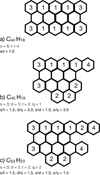 |
Fig. 30 Illustration of molecules depicting the various types of peripheral CH groups in PAHs in the Orion Bar. The counts of of solo, duo, trio, and quartet functional groups are denoted as s, d, t, and q, respectively. The numbers on the rings in each structure indicate the number of adjacent CH groups attached to each ring. Structure (a) satisfies the s/t CH group ratio, derived for the PDR. Structures (b) and (c), satisfy the s/t and d/q ratios derived for the atomic PDR and DF 3 of the Orion Bar, respectively. |
6.3 Very small grains in the Orion Bar
Carbonaceous VSGs, are another class of mid-IR AIB carriers prevalent in the ISM. In one chemical scenario, VSGs have been proposed to undergo photo-evaporation under UV radiation at the surfaces of PDRs, to produce free-flying PAHs (Cesarsky et al. 2000). Indeed, analyzing mid-IR emission spectra from myriad objects, Rapacioli et al. (2005) and Berné et al. (2007) were able to extract three independent spectra belonging to two populations: PAH molecules (neutral and ionized) and VSGs. Rapacioli et al. (2005) suggested that these grains are PAH clusters. VSGs have been hypothesized to photoevaporate by intense UV radiation, and thereby undergo unique physico-chemical processing and evolution in PDRs (Rapacioli et al. 2006; Pilleri et al. 2012).
In the narrative of carbonaceous molecules present in the Orion Bar PDR, VSGs have been introduced as another family of key actors. Following Pasquini et al. (2024) and Chown et al. (2024), we attribute the 11.25 µm component observed at large distances from the Orion Bar PDR surface to VSGs and/or PAH clusters and the 11.207 µm AIB to monomeric PAH. The distinct spatial distributions of these two AIBs agree with the results obtained by Rapacioli et al. (2005) and Berné et al. (2007) based on ISO and Spitzer observations of a large sample of objects. We follow their interpretation that the more labile PAH clusters are broken down to free-flying PAHs when advected through the PDR. Experimental and theoretical studies have shown that the CHoop modes are redshifted and broadened in PAH clusters (Ricca et al. 2013; Roser & Ricca 2015), further supporting our assignment of the 11.207 µm and 11.25 µm components to solo CHoop modes in monomeric PAHs and PAH clusters, respectively.
Within the assembly of 10–15 µm AIBs, we find that VSGs contribute to another AIB, besides the 11.25 µm band. Indeed, we find that the six Gaussian components of the 12.0 µm AIB are all strongly related to the 11.25 µm band, and thus have significant contributions from VSGs. Guided by this knowledge, we performed a decomposition of the 12.0 µm AIB using the 11.207 and 11.25 µm AIB maps. Unlike for the 12.7 µm AIB, such a decomposition results in excellent fits of the nominal 12.0 µm profile confirming the contribution of both carriers. As a consequence, the resulting 12.02 component at ∼ 11.92 µm, is found to be in good likeness in morphology to the 11.25 µm band. We note however that unlike the 11.25 µm band, the ∼ 11.92 µm 12.02 component lies at a shorter wavelength than the nominal AIB at 12.0 µm.
A PCA of the surface brightnesses of the 10–15 µm AIBs, and components of the 11.2, 12.7 and 12.0 µm AIBs also reveals the 11.25 µm and 12.02 bands to be clear outliers. Indeed, variations in the overall strength of the PAH emission in the Orion Bar are captured within the first principal component, PC1. In contrast, the second uncorrelated principal component, PC2, is strongly associated with the surface brightnesses of the 11.25 µm and 12.02 µm components. The six spectral components in which the 12.0 µm AIB is decomposed into, also exhibit larger contributions to PC2, than the other AIBs. This indicates that PC2 variations reflect the degree of contributions of VSGs to the AIBs. While the strength of the relatively weak 12.0 µm AIB is influenced by the spectral decomposition which employs a 11–14 µm broad plateau, other spectral decompositions (including those not employing a broad underlying plateau) will extract an 12.0 µm AIB which completely encompasses the 12.0 µm AIB derived in this work. As a consequence, VSGs and/or PAH clusters will also contribute to the 12.0 µm AIBs derived with alternative decompositions, albeit with a different relative contribution with respect to PAHs. Furthermore, the 11–14 µm broad plateau has also been hypothesized to arise from VSGs (Berné et al. 2007; Foschino et al. 2019). We apply a PCA on the main AIBs and this measured broad 10–15 µm plateau. The biplot shown in Fig. D.10 reveals that this plateau contributes to both PC1 and PC2, and is thus a mixture of free-flying PAHs and carbonaceous grains. These findings underscore the potential for distinguishing the spectral signatures of PAH monomers versus VSGs and/or PAH clusters in the 10–15 µm spectral region.
7 Conclusions
The outstanding PDRs4All JWST MIRI-MRS IFU spectro-scopic observations of the archetypal PDR, the Orion Bar, have unveiled the profound nuances within the spatial and spectral behavior of AIBs in the 10–15 µm spectral domain. These AIBs are largely attributed to vibrational CH out-of-plane bending modes in PAHs. A plethora of AIBs at 10.6, 10.8, 11.0, 11.2, 12.0, 12.7, 13.5, 14.0, and 14.2 µm are observed. We present spatial-spectral maps of the measured surface brightnesses of all AIBs in this cohort. All 10–15 µm AIBs share similar large-scale behavior: the AIB emission peaks in the atomic PDR of the Orion Bar close to the IF, declines gradually with distance away from the IF, and exhibits pronounced peaks, most notably for the 11.2, 12.0, and 13.5 µm AIBs, in the H I/H2 dissociation fronts. The AIBs also display smaller-scale spatial variations in their emission, primarily in the atomic PDR. The global and local trends in the AIB morphologies result from an amalgamation of the strength of the local UV radiation field within the Orion Bar, the population of the PAHs, and the effects of column density along the line of sight toward the edge-on PDR.
We have showcased the intricacies and richness of the spectral profiles of the traditional 11.2 µm and 12.7 µm AIB complexes in the observed spectra, and presented their decompositions. We also observed notable spectral variations in the 12.0 µm and 13.5 µm AIBs, and decomposed the 12.0 µm AIB to investigate the enhanced emission of this band in the molecular PDR and its tight correlation with the 11.25 µm AIB. The 11.2 µm AIB is found to comprise two independent components at 11.207 µm and ∼ 11.25 µm, which exhibit distinctly different spatial distributions, along with an additional component that peaks at ∼ 11.22 µm, but eludes measurement. The 11.207 µm component is the dominant contributor to the aggregate 11.2 µm band, while the 11.25 µm band primarily contributes to the 11.2 µm AIB in DF 3. We identify a component of the 12.0 µm AIB at ∼ 11.90 µm, which correlates strongly with the 11.25 µm band. We have introduced a six-Gaussian mixture model of the 12.7 µm AIB. The four components between 12.36–12.75 µm resemble each other in morphologies, while the latter two components at 12.805 µm and 12.96 µm together display slightly different small-scale structures than the other components. Based on this simple decomposition, the bulk emission of the 12.7 µm AIB is carried by the two components, at 12.71 µm and 12.805 µm.
Investigating the correlations of the AIBs’ surface brightnesses, we find them all to be strongly correlated. The strongest positive correlation is found between the 11.0 µm and 11.207 µm AIB surface brightnesses. Among surface brightnesses normalized to the 11.207 µm AIB, the 13.5 µm, 12.0 µm, and 11.0 µm AIBs show the strongest mutual correlations.
We hypothesize the following origins for the AIBs studied in this work. The correlations along with a statistical PCA, designed to explore the uncorrelated drivers of variation in the data, confirm the presence of two distinct populations of AIB carriers in the Orion Bar: PAHs and VSGs and/or PAH clusters. The 11.25 µm AIB and the resembling component at ∼ 11.90 µm within the 12.0 µm AIB are hypothesized to be carried by VSGs and/or PAH clusters thriving in the molecular PDR, where they are shielded from photo-destruction, whereas all other AIBs are dominated by vibrations in FUV-excited PAHs. We attribute the 11.0 µm and 11.207 µm AIBs to solo CHoop vibrations in cationic and neutral PAHs, respectively. The duo CHoop mode in PAHs with solo and duo hydrogens splits into two modes, referred to as duo1 and duo2 (Bauschlicher et al. 2009). The 12.01 µm component of the 12.0 µm AIB is assigned to the duo1 mode, whereas the 12.55 µm and 12.62 µm components of the 12.7 µm AIB complex are assigned to the duo2 mode in irregular PAHs, and the 12.96 µm component is assigned to duo2 mode in compact PAHs. The trio CHoop mode contributes to the bulk of the surface brightness of the 12.7 µm AIB in compact PAHs, carried by the subcomponents at 12.36, 12.55, 12.62, 12.71, and 12.805 µm. Thus, the 12.7 µm AIB complex has contributions from out-of-plane bending of both duo and trio hydrogens in PAHs. The JWST observations have thus revealed the spectrally complex components of the 12.0, 12.7, and 13.5 µm AIBs. Rigorous assignment of these subcomponents to PAH spectral modes requires further experimental and theoretical work on a broader range of PAHs.
We utilized theoretical and observed band strengths to constrain the relative number of solo, duo, trio, and quartet CH groups in the PAHs inhabiting the Orion Bar. The relative number of s/t and d/q CH groups is consistent across the PDR, where the d/q ratios are slightly larger than the s/t ratios. We propose that the PAH family in the Orion Bar consists of members with compact, symmetric structures, rich in solo and trio edge hydrogens, with variable labile CH side-groups of duos and quartets that are lost near the PDR surface via photo-processing.
Evidently, JWST’s remarkable capabilities have revolutionized our ability to finely probe the structures and fates of widespread carbonaceous species, such as the renowned PAH family, in their cosmic environments. The Orion Bar, seen through JWST’s powerful mirror, offers an ideal laboratory for this exploration.
Acknowledgements
This work is based on observations made with the NASA/ESA/CSA James Webb Space Telescope. The data were obtained from the Mikulski Archive for Space Telescopes at the Space Telescope Science Institute, which is operated by the Association of Universities for Research in Astronomy, Inc., under NASA contract NAS 5-03127 for JWST. These observations are associated with program #1288 (DOI: 10.17909/pg4c-1737). Support for program #1288 was provided by NASA through a grant from the Space Telescope Science Institute, which is operated by the Association of Universities for Research in Astronomy, Inc., under NASA contract NAS 5-03127. Baria Khan is grateful for the support from the University of Western Ontario, and the Government of Ontario, through the Ontario Graduate Scholarship. Benjamin Abbott gratefully acknowledges the MITACS Globalink Research Internship and the University of Western Ontario for hosting. Els Peeters and Jan Cami acknowledge support from the University of Western Ontario, the Canadian Space Agency (CSA, 22JWGO1-16), and the Natural Sciences and Engineering Research Council of Canada. This article is based upon work from COST Action CA21126 – Carbon molecular nanostructures in space (NanoSpace), supported by COST (European Cooperation in Science and Technology). Takashi Onaka acknowledges the support by the Japan Society for the Promotion of Science (JSPS) KAKENHI Grant Number JP24K07087. Christiaan Boersma is grateful for an appointment at NASA Ames Research Center through the San José State University Research Foundation (80NSSC22M0107). Mridusmita Buragohain thanks the DST INSPIRE Faculty fellowship for awarding her research fellowship and the Inter-University Centre for Astronomy and Astrophysics, Pune for visiting associateship.
Appendix A Spectral decompositions of the 12.7 µm and 12.0 µm AIBs
To systematically investigate the presence and behavior of the six components of the 12.7 µm complex, we adopt a similar decomposition methodology as Shannon et al. (2016). We utilize the curve_fit function from the optimize module in the Python Scipy library to perform non-linear least squares regression to fit a 12-Gaussian model to the data. The first six Gaussians fit the H2 line, four H I emission lines and the [Ne II] line, for all of which the centers (µ) and standard deviations (σ) were kept fixed (Table A.1). These fixed parameters are informed by the best fit for each line in the five template spectra, using wave-lengths from the list of mid-IR emission lines provided by Van De Putte et al. (2024) and the MIRI-MRS spectral resolution at the given wavelengths. The rest of the model consists of the sum of six broad Gaussians over the breadth of the spectrum between 12.2–13.1 µm to fit the 12.7 µm AIB. We first perform a series of “unconstrained” model fitting, where the initial values of centers, standard deviations and amplitudes of these six Gaussian components and the amplitudes of the six line Gaussians are provided. Bounds are imposed on the centers and widths of the component Gaussians, when necessary, to minimize overlap and improve the quality of these unrestricted fits. We inspect the modes in the histograms of the peaks and widths of the six component Gaussians to inform the selection of initial parameters for the next round of fitting. Thus, multiple iterations of these fitting routines result in convergence of these parameters to distinct values that are given in Table A.1. Thereafter, we performed “constrained fits” whereby the peak position and FWHM (σ) parameters were fixed to these values for all components.
We decompose the 12.0 AIB into six components, adopting the same methodology as for the 12.7 µm AIB. The parameters used for the fits are given in Table A.1.
Parameters used for the 12.7 µm AIB decomposition (left) and the 12.0 µm AIB decomposition (right).
Appendix B Morphology of the 12.7 µm and 12.0 µm AIB components
Figures B.1 and B.2 display the spatial maps for the spectral components for the 12.7 µm and 12.0 µm AIBs (see Sects. 5.4 and 5.5.1, respectively).
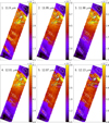 |
Fig. B.2 Spatial distribution of the six 12.0 µm AIB subcomponents, introduced in Sect. 5.5.1. |
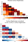 |
Fig. C.1 The heat map of pairwise correlation coefficients R of the surface brightnesses of AIBs with SNR > 3 from the PDR (i.e., excluding the H II region) for absolute surface brightnesses (top) and for surface brightnesses normalized to the 11.207 µm surface brightnesses (bottom). |
Appendix C Correlation coefficients and additional correlation plots
We find clear correlations in absolute surface brightnesses of the 10.6, 10.8, 12.0, 12.7, 13.5, 14.0, and 14.2 µm AIBs with the 11.2 µm AIB surface brightness (Figs. C.1 and C.2). This suggests that all bands considered in this paper belong to the AIB family. We present color-coded “heat” matrices of computed Spearman correlation coefficients “R” between the measured surface brightnesses of the AIBs and between the surface brightnesses of the AIBs normalized to the 11.207 µm surface brightness (Fig. C.1). In addition, we find strong correlations between the 12.805 and 12.96 µm components and the 11.207 µm component when normalized on the 11.0 µm AIB (Fig. C.3). Such strong correlations indicate that both the 12.805 µm and 12.96 µm subcomponents of the 12.7 µm AIB originate in neutral PAHs.
Appendix D Principal component analyses
We describe the mathematical formalism of the PCA, the input for the different PCA iterations and their results.
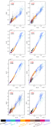 |
Fig. C.2 Correlations of 10–15 µm AIBs with the 11.2 µm AIB surface brightnesses. The correlation coefficient, R, for the variables excluding and including the points from the H II region (black), are listed in red and black, respectively. The data points are colored according to regions in the mosaic where those pixels are located, per the color bar. |
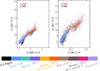 |
Fig. C.3 Correlations of the 12.805 and 12.96 µm surface brightnesses with the 11.207 µm surface brightnesses, normalized to the 11.0 µm surface brightnesses. The correlation coefficient, R, for the variables excluding and including the points from the H II region are listed in red and black, respectively. The data points are colored according to regions in the mosaic where those pixels are located, per the color bar at the bottom. |
Appendix D.1 Methodology
Principal component analysis is a data analysis technique used to investigate large, complex data by restructuring the components into a new set of uncorrelated variables, referred to as the principal components (PCs). The first principal component explains the majority of the variations in the data, the second component explains the second-largest variation, and so forth. The following PCs then have decreasing levels of variance to a point where they can be considered to have negligible influence in explaining the statistics of the data.
In a traditional PCA, a standardization of the data is performed first so that each input component carries an equal weight in the analysis. This effectively prevents certain numerically stronger inputs from dominating and obscuring the minor trends. We have set all data variables to have a mean of zero and a unit standard deviation, further referred to as standardized input variables:
![Mathematical equation: \[{z_{jk}} = \left( {{I_{jk}} - \langle {I_j}\rangle } \right)/{\sigma _j}\]](/articles/aa/full_html/2025/07/aa54096-25/aa54096-25-eq8.png)
where I jk is the surface brightness of AIB j at spaxel k, and ⟨I j⟩ and σ j the mean and standard deviation, respectively, of the surface brightnesses of AIB j across the mosaic. Next, the principal components are calculated as the (dimensionless) eigenvectors of the covariance matrix formed from the standardized input variables. The eigenvalues of these vectors represent the variance. The order of the PCs is defined in terms of decreasing eigenvalues. As these PCs are eigenvectors of a covariance matrix, they are completely orthogonal to each other; that is, they are independent from one another (for more details on the mathematical framework, we refer the reader to Sidhu et al. (2021)).
Appendix D.2 Input for PCA
We performed PCA on various input variables (referred to as rounds). The AIBs’ surface brightnesses were used as the standard inputs for the PCA. For each round, slight alterations were made to this input list; for example, by including subcomponents as follows:
Considering the components of the 11.2 µm AIB decomposition (11.207 and 11.25 µm AIBs), and the rest of the AIBs (10.6, 10.8, 11.0, 12.0, 12.7, 13.5, 14.0, and 14.2 µm)
Considering the components of the 11.2 and 12.7 µm AIBs decompositions, the components of the Gaussian mixture model decomposition of the 12.0 µm, decomposition, and the rest of the AIBs (10.6, 10.8, 11.0, 13.5, 14.0, and 14.2 µm)
Considering the components of the 11.2 and 12.7 µm AIBs decompositions, the two components of the second 12.0 µm decomposition, and the rest of the AIBs (10.6, 10.8, 11.0, 13.5, 14.0, and 14.2 μm)
Considering the standard AIBs (without any decomposition)
Before applying the PCA, the surface brightnesses with an SNR < 3, from the proplyds, and the H II region are masked. Table D.1 gives the input standardized surface brightness values (zAIB) for each round. Table D.2 gives the fractional variances explained by the first three principal components for each round. We do not consider the principal components beyond the third one, as the first three components explain ∼ 99% of the variance. The principal components can be described as linear combinations of these standardized surface brightness variables, their coefficients for each round are given in Table D.3.
The mean (⟨IAIB⟩) and standard deviation (σAIB) values of the input AIB variables, in the four PCA rounds.
The variance in each PC for each round.
Contribution αi j of each standardized AIB, z j, to the principal components PCi: PCi = Σ j αi j z j and z j = Σi αi j PCi.
Appendix D.3 Results of PCA round 1
In this round, the PCA is applied on the surface brightnesses of the 10.6, 10.8, 11.0, 11.207, 11.25, 12.0, 12.7, 13.5, 14.0, 14.2 µm AIBs. The spatial morphologies of the three PCs are clearly distinct (Fig. D.1). Although large around the IF, PC3 appears to mainly trace the noise in the data. Figure D.2 displays the biplots that show the contribution of each standardized component to each principal component via projections on the axes of the respective principal component. In the PC1-PC2 plane, all the standardized input variables except for the 11.25 µm AIB display a positive projection on PC1. Indeed, PC1 linearly correlates very well with 11.207 µm surface brightness and the sum of the input surface brightnesses excluding the the 11.25 µm surface brightnesses (Fig. D.3).The 11.25 µm AIB displays an almost orthogonal projection on PC2 suggesting that it is independent of the others AIBs and represented almost entirely by PC2. Despite having strong projections on to PC1, the 12.0 µm and 13.5 µm AIBs also have similarly significant weighted projections on to PC2 indicating that certain variations within these AIBs are better explained by PC2. Indeed, PC2 correlates very well with the 11.25 µm surface brightness and the 12.0 and 13.5 µm band surface brightnesses arising from the molecular PDR also correlate linearly with PC2 (Fig. D.3). Finally, in the PC1-PC2 plane, the 10.6, 10.8, and 13.5 µm AIBs have the largest projections on to PC3 (Fig. D.2). However, this PC explains less than 2% of the variance in the surface brightnesses of the AIBs (Table D.2), so a physical meaning cannot be extracted for PC3.
This PCA round thus demonstrates that the 11.25 µm AIB is atypical than the principal AIBs, and stands out distinctly in such a statistical analysis.
Appendix D.4 Results of PCA round 2
In this round, the PCA is applied on the surface brightnesses of the 10.6, 10.8, 11.0, 11.207, 11.25, 11.9, 11.95, 11.98, 12.01, 12.07, 12.13, 12.36, 12.55, 12.62, 12.71, 12.805, 12.96, 13.5, 14.0, and 14.2 µm AIBs. The spatial morphology of the PCs and the biplots are presented in Figs. D.4 and D.5. Similarly to round 1, all AIBs except the 11.25 µm AIB correlate positively with PC1, indicating their common origin in PAH fluorescence. However, the six Gaussian components of the 12.0 µm AIB, as well as of the 13.5 µm AIB, have larger positive projections on the PC2 axis, compared to the rest of the AIBs. The projection on the PC2 axis of the Gaussian components of the 12.7 µm AIB is quite diverse. In contrast to round 1, PC1 does not have a strict linear relationship with the cumulative surface brightnesses of the AIBs and with the 11.207 µm AIB when eliminating the 11.25 µm AIB and the correlation between PC2 and the 11.25 µm AIB is weaker (Fig. D.6).
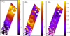 |
Fig. D.1 Spatial distribution of the PCs from round 1. |
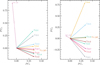 |
Fig. D.2 Biplots for the PCA round 1. Biplots show the projection of the standardized input variables on to the PCi axes. |
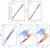 |
Fig. D.3 Selected correlation plots for the PCA round 1. |
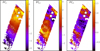 |
Fig. D.4 Spatial maps for the PCs from PCA round 2. |
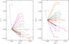 |
Fig. D.5 Biplots for the PCA round 2. |
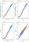 |
Fig. D.6 Selected correlation plots for the PCA round 2. |
This PCA demonstrates that the Gaussian decompositions of the 12.0 µm and 12.7 µm AIBs do not yield any entirely independent component(s) akin to the 11.25 µm component, which is distinctly singled out as an outlier through this PCA, and the PCA round 1(D.3).
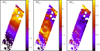 |
Fig. D.7 Spatial maps for the PCs from PCA round 3. |
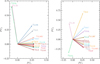 |
Fig. D.8 Biplots for the PCA round 3. |
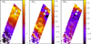 |
Fig. D.9 Spatial distribution of the PCs from round 4. |
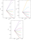 |
Fig. D.10 Biplots for the PCA round 4. The bottom panel shows the PC1 vs. PC2 biplot when the broad 10–15 µm plateau (Fig. 3) is included. Biplots show the projection of the standardized input variables on to the PCi axes. |
Appendix D.5 Results of PCA round 3
In this round, the PCA is applied on the surface brightnesses of the 10.6, 10.8, 11.0, 11.207, 11.25, 12.01, 12.02, 12.36, 12.55, 12.62, 12.71, 12.805, 12.96, 13.5, 14.0, and 14.2 µm AIB. Figs. D.7 and D.8 display the maps of the PCs and the biplots. We disregard the behavior of PC3, since it explains less than 1.4% of the variance in the data (Table D.2).
The results for round 3 are discussed in detail in Sect. 5.8. In summary, in addition to the 11.25 µm component, the 12.02 component from the spectral map-fitting decomposition of the 12.0 µm AIB, now also appears as an outlier(D.8). PC1 thus traces typical PAH emission, while PC2 traces emission independent of it.
Appendix D.6 Results of PCA round 4
In this round, the PCA is applied on the surface brightnesses of the original AIBs at 10.6, 10.8, 11.0, 11.2, 12.0, 12.7 13.5, 14.0, and 14.2 µm. The maps of the PCs and biplots are presented in Figs. D.9 and D.10. All AIBs correlate positively with PC1, indicating their common origin in PAH fluorescence. The projection on PC2 divides the AIBs in three groups: 1. the 12.0 and 13.5 µm AIBs have the largest positive PC2 projections; 2. the 10.6, 10.8, 11.2, and 12.7 AIBs have PC2 projections near zero; and 3. the 11.0, 14.0, and 14.2 µm AIBs have negative PC2 projections.
This PCA round demonstrates that PC1 lends support to the common origin of these AIBs, while PC2 correlates well with AIBs (12.0, 13.5, 10.8 and 11.2 µm) that have been observed to have pronounced emission in the molecular PDR (Fig. 5).
Appendix E Peculiarities of the 11.25 µm AIB morphology
In this section we investigate the curious behavior of 11.25 µm emission from VSGs and/or PAH clusters near the IF at the precipice of the Orion Bar. An enhancement in the 11.25 µm emission is observed along a narrow “ridge” just past the IF, on the north-western end of the FOV (Fig. E.1). This region is also visibly brighter in the map of the anomalous 12.02 component from the 12.0 µm AIB (Fig. 21). Therefore, we inspected a few spectra perpendicular to the IF, from above, within, and below this ridge (Fig. E.2). The prominence of the 11.25 µm component in the 11.2 µm profile is indeed “sudden” in the pixels that lie just below the IF that belong to this ridge of interest. The peak at ∼ 11.25 µm does indeed drop right around this region in the atomic PDR. Since it is highly implausible for VSGs and/or PAH clusters to survive in this region of harsh FUV radiation at the onset of the PDR, the observations of these large 11.25 µm surface brightnesses just past the IF are odd. It is possible that this close agreement between the 11.25 µm surface brightnesses from this region of interest and DF 2 in particular may be a product of the deficiencies in the 11.2 µm decomposition we adopt. Yet, we find a remarkable similitude in the spectral characteristics of the 11.2 µm AIB profiles near the IF and DF 2 (Fig. E.2) - regions with vast differences in physical and chemical conditions.
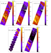 |
Fig. E.1 Spatial distribution of the surface brightness [W m−2 sr−1] of the 11.25 µm AIB, the 11.25/11.207 µm and 11.25/11.2 µm surface brightness ratios, the O I 1.317 µm fluorescence line [erg cm−2 s−1 sr−1] from Peeters et al. (2024), and the H2 0-0 S(3) line [W m−2 sr−1] at 9.664 µm from Sidhu et al. (in prep.). The black contours in the top right panel correspond to I11.25 = 1.25 × 10⁻⁵ W m−2 sr−1. In the top middle and right panels, the white and teal contours trace peak emission for the 11.0 µm and the 11.2 µm band, respectively, and the black contour corresponds to a 11.25/11.207 ratio of 0.8. In the bottom left panel, the dashed black line represents the “secondary ridge” discussed in the text. θ1 Ori C is located toward the top right of each map (see Fig. 2). In each map the range of the corresponding color bar is set between 0.5% and 99.5% percentile level for the data. The zero pixels, and in the maps based on the MIRI FOV, the edge pixels, and pixels covering the two proplyds, indicated by the black circles, are masked out. The rectangular apertures of the template spectra for the H II region, atomic PDR, DF 1, DF 2, and DF 3, from top to bottom, are shown in white and the solid white lines delineate the IF and the three DFs, DF 1, DF 2 and DF 3. |
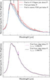 |
Fig. E.2 Illustration of the 11.2 µm profiles normalized to their peak specific surface brightnesses near the IF. Top: profiles, in groups of three, of the pixels that are marked by ⋆ symbols on the 11.25 µm map in Fig. E.1. Bottom: profiles from a pixel marked by a × symbol in purple near the IF and a pixel marked by a × symbol in black DF 2 in the 11.25 µm map in Fig. E.1. |
Akin to this bright 11.25 µm ridge near the IF, a bright “full” ridge is noticed in the O I 1.317 µm fluorescence line emission (Fig. E.1, Peeters et al. 2024). This line’s strength peaks just beyond the IF and the emission drops sharply with increasing distance from the IF. Peeters et al. (2024) note that the O I 1.317 µm morphology exhibits a secondary, slightly weaker ridge, south of the primary ridge. The bright 11.25 µm emission just beyond the IF appears to be contained within this secondary ridge seen in O I 1.317 µm. We further notice the absence of any similar elevated emission in any of the maps of the H2 lines (Fig. E.1).
Altogether, we surmise that this increased 11.25 µm emission near the IF reflects line-of-sight confusion of the background (H II region) PDR extending slightly behind the Orion Bar PDR. However, in that case if this 11.25 µm emission indeed comes from a background molecular PDR, by analogy with DF 2/DF 3, some enhanced H2 emission would also be expected, but is absent in the observations. Evidently, the peculiar behavior of the 11.25 µm emission requires further investigation.
Appendix F Correlation plots including the H II region
In this section we present the version of the correlation plots shown in the main text, which includes spaxels from the H II region. The surface brightnesses from the H II region and beyond DF 3, often lie displaced from the main trends in these correlation plots. Following Sect. 6.2, we derive s/d, s/t, and s/q ratios of 18.8, 1.8, and 41.2 respectively for the H II region.
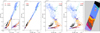 |
Fig. F.1 Correlations plots of the 11.0, 11.2, 11.207, and 11.25 µm surface brightnesses in units of W m−2 sr−1. The correlation coefficient “R” for the variables excluding (including) the points from the H II region (black), are listed in red (black). The colored star symbols represent the five template spectra from the PDR (H II region: black, atomic PDR: blue; DF 1: purple; DF 2: orange; and DF 3: pink). Only surface brightnesses with SNR > 3 from every other spaxel are considered. The data points are colored according to regions in the mosaic where those pixels are located (fifth panel): black (H II region), blue (atomic PDR), teal (west IF), purple (DF 1), yellow (region between DF 1 and DF 2), orange (DF 2), light brown (region west of DF 2), brown (region between DF 2 and DF 3), pink (DF 3) and light purple (region beyond DF 3). The contours highlighting DF 2 and DF 3 are identified through enhanced emission of H2 0-0 S(3) in these DFs. The red circular regions on the color-region map (fifth panel) correspond to the proplyds, as these pixels have been masked in our data analysis. |
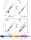 |
Fig. F.2 Noteworthy correlations for the 12.0 µm AIB and its components. The correlation coefficient, R, for the variables excluding (including) the points from the H II region (black), are listed in red (black). The data points are colored according to regions in the mosaic, per the color bar at the bottom. |
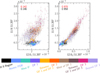 |
Fig. F.3 Correlations of the 12.0-G1 (11.90 µm) subcomponent with the 12.01 and 12.02 components. The correlation coefficient, R, for the variables excluding (including) the points from the H II region (black), are listed in red (black). The data points are colored according to regions in the mosaic, per the color bar at the bottom. |
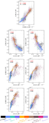 |
Fig. F.4 Correlation plots for the 12.805 µm and 12.96 µm components of the 12.7 µm AIB. The correlation coefficient, R, for the variables excluding (including) the points from the H II region (black), are listed in red (black). The data points are colored according to regions in the mosaic, per the color bar at the bottom. |
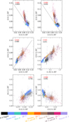 |
Fig. F.5 Correlation plots for the 13.5, 12.0, and 14.2 µm bands normalized to the 11.207 µm AIB. The correlation coefficient, R, for the variables excluding (including) the points from the H II region (black), are listed in red (black). The data points are colored according to regions in the mosaic, per the color bar at the bottom. |
References
- Allamandola, L. J., Tielens, A. G. G. M., & Barker, J. R. 1985, ApJ, 290, L25 [Google Scholar]
- Allamandola, L. J., Hudgins, D. M., & Sandford, S. A. 1999, ApJ, 511, L115 [Google Scholar]
- Andrews, H., Candian, A., & Tielens, A. G. G. M. 2016, A&A, 595, A23 [NASA ADS] [CrossRef] [EDP Sciences] [Google Scholar]
- Argyriou, I., Glasse, A., Law, D. R., et al. 2023, A&A, 675, A111 [NASA ADS] [CrossRef] [EDP Sciences] [Google Scholar]
- Bakes, E. L. O., & Tielens, A. G. G. M. 1994, ApJ, 427, 822 [NASA ADS] [CrossRef] [Google Scholar]
- Bakker, J. M., Redlich, B., van der Meer, A. F. G., & Oomens, J. 2011, ApJ, 741, 74 [Google Scholar]
- Bally, J. 2008, arXiv e-prints [arXiv:0812.0046] [Google Scholar]
- Bauschlicher, Charles W. J., Peeters, E., & Allamandola, L. J. 2008, ApJ, 678, 316 [NASA ADS] [CrossRef] [Google Scholar]
- Bauschlicher, Charles W. J., Peeters, E., & Allamandola, L. J. 2009, ApJ, 697, 311 [NASA ADS] [CrossRef] [Google Scholar]
- Bauschlicher, Jr., C. W., Boersma, C., Ricca, A., et al. 2010, ApJS, 189, 341 [NASA ADS] [CrossRef] [Google Scholar]
- Bauschlicher, Jr., C. W., Ricca, A., Boersma, C., & Allamandola, L. J. 2018, ApJS, 234, 32 [NASA ADS] [CrossRef] [Google Scholar]
- Bellamy, L. 1975, The Infra-red Spectra of Complex Molecules (London: Chapman and Hall) [CrossRef] [Google Scholar]
- Berné, O., Joblin, C., Deville, Y., et al. 2007, A&A, 469, 575 [NASA ADS] [CrossRef] [EDP Sciences] [Google Scholar]
- Berné, O., Habart, É., Peeters, E., et al. 2022, PASP, 134, 054301 [CrossRef] [Google Scholar]
- Boersma, C., Bauschlicher, Jr., C. W., Ricca, A., et al. 2014, ApJS, 211, 8 [NASA ADS] [CrossRef] [Google Scholar]
- Boersma, C., Bregman, J., & Allamandola, L. J. 2016, ApJ, 832, 51 [NASA ADS] [CrossRef] [Google Scholar]
- Califano, S. 1962, J. Chem. Phys., 36, 903 [Google Scholar]
- Candian, A., Sarre, P. J., & Tielens, A. G. G. M. 2014, ApJ, 791, L10 [CrossRef] [Google Scholar]
- Castellanos, P., Candian, A., Zhen, J., Linnartz, H., & Tielens, A. G. G. M. 2018, A&A, 616, A166 [NASA ADS] [CrossRef] [EDP Sciences] [Google Scholar]
- Cesarsky, D., Lequeux, J., Ryter, C., & Gérin, M. 2000, A&A, 354, L87 [Google Scholar]
- Chown, R., Sidhu, A., Peeters, E., et al. 2024, A&A, 685, A75 [NASA ADS] [CrossRef] [EDP Sciences] [Google Scholar]
- Cohen, M., Allamandola, L., Tielens, A. G. G. M., et al. 1986, ApJ, 302, 737 [Google Scholar]
- Elliott, K. H., & Meaburn, J. 1974, Ap&SS, 28, 351 [NASA ADS] [CrossRef] [Google Scholar]
- Foschino, S., Berné, O., & Joblin, C. 2019, A&A, 632, A84 [EDP Sciences] [Google Scholar]
- Genzel, R., Lutz, D., Sturm, E., et al. 1998, ApJ, 498, 579 [Google Scholar]
- Gillett, F. C., Forrest, W. J., & Merrill, K. M. 1973, ApJ, 183, 87 [NASA ADS] [CrossRef] [Google Scholar]
- Goicoechea, J. R., Pety, J., Cuadrado, S., et al. 2016, Nature, 537, 207 [Google Scholar]
- Goicoechea, J. R., Pety, J., Cuadrado, S., et al. 2025, A&A, 696, A100 [NASA ADS] [CrossRef] [EDP Sciences] [Google Scholar]
- Habart, E., Peeters, E., Berné, O., et al. 2024, A&A, 685, A73 [NASA ADS] [CrossRef] [EDP Sciences] [Google Scholar]
- Habing, H. J. 1968, Bull. Astron. Inst. Netherlands, 19, 421 [Google Scholar]
- Hony, S., Van Kerckhoven, C., Peeters, E., et al. 2001, A&A, 370, 1030 [CrossRef] [EDP Sciences] [Google Scholar]
- Hudgins, D. M., & Allamandola, L. J. 1999, ApJ, 516, L41 [CrossRef] [Google Scholar]
- Knight, C., Peeters, E., Tielens, A. G. G. M., & Vacca, W. D. 2022, MNRAS, 509, 3523 [Google Scholar]
- Langhoff, S. R. 1996, J. Phys. Chem., 100, 2819 [Google Scholar]
- Law, D. R., E Morrison, J., Argyriou, I., et al. 2023, AJ, 166, 45 [NASA ADS] [CrossRef] [Google Scholar]
- Leger, A., & Puget, J. L. 1984, A&A, 137, L5 [Google Scholar]
- Lemmens, A. K., Rijs, A. M., & Buma, W. J. 2021, ApJ, 923, 238 [NASA ADS] [CrossRef] [Google Scholar]
- Mackie, C. J., Candian, A., Lee, T. J., & Tielens, A. G. G. M. 2022, J. Phys. Chem. A, 126, 3198 [CrossRef] [Google Scholar]
- Maragkoudakis, A., Boersma, C., Temi, P., et al. 2025, ApJ, 979, 90 [Google Scholar]
- Matsuura, M., Bernard-Salas, J., Lloyd Evans, T., et al. 2014, MNRAS, 439, 1472 [NASA ADS] [CrossRef] [Google Scholar]
- Menten, K. M., Reid, M. J., Forbrich, J., & Brunthaler, A. 2007, A&A, 474, 515 [NASA ADS] [CrossRef] [EDP Sciences] [Google Scholar]
- O’Dell, C. R. 2001, ARA&A, 39, 99 [Google Scholar]
- O’Dell, C. R., Kollatschny, W., & Ferland, G. J. 2017, ApJ, 837, 151 [CrossRef] [Google Scholar]
- O’Dell, C. R., Abel, N. P., & Ferland, G. J. 2020, ApJ, 891, 46 [CrossRef] [Google Scholar]
- Oomens, J., Tielens, A. G. G. M., Sartakov, B. G., von Helden, G., & Meijer, G. 2003, ApJ, 591, 968 [Google Scholar]
- Pabst, C., Higgins, R., Goicoechea, J. R., et al. 2019, Nature, 565, 618 [NASA ADS] [CrossRef] [Google Scholar]
- Panchagnula, S., Bouwman, J., Rap, D. B., et al. 2020, Phys. Chem. Chem. Phys. (Incorp. Faraday Trans.), 22, 21651 [Google Scholar]
- Pasquini, S., Peeters, E., Schefter, B., et al. 2024, A&A, 685, A77 [NASA ADS] [CrossRef] [EDP Sciences] [Google Scholar]
- Peeters, E., Hony, S., Van Kerckhoven, C., et al. 2002, A&A, 390, 1089 [NASA ADS] [CrossRef] [EDP Sciences] [Google Scholar]
- Peeters, E., Bauschlicher Charles W. J., Allamandola, L. J., et al. 2017, ApJ, 836, 198 [NASA ADS] [CrossRef] [Google Scholar]
- Peeters, E., Habart, E., Berné, O., et al. 2024, A&A, 685, A74 [NASA ADS] [CrossRef] [EDP Sciences] [Google Scholar]
- Pellegrini, E. W., Baldwin, J. A., Ferland, G. J., Shaw, G., & Heathcote, S. 2009, ApJ, 693, 285 [CrossRef] [Google Scholar]
- Pilleri, P., Montillaud, J., Berné, O., & Joblin, C. 2012, A&A, 542, A69 [NASA ADS] [CrossRef] [EDP Sciences] [Google Scholar]
- Rapacioli, M., Joblin, C., & Boissel, P. 2005, A&A, 429, 193 [NASA ADS] [CrossRef] [EDP Sciences] [Google Scholar]
- Rapacioli, M., Calvo, F., Joblin, C., et al. 2006, A&A, 460, 519 [NASA ADS] [CrossRef] [EDP Sciences] [Google Scholar]
- Ricca, A., Bauschlicher Charles W. J., Boersma, C., Tielens, A. G. G. M., & Allamandola, L. J. 2012, ApJ, 754, 75 [NASA ADS] [CrossRef] [Google Scholar]
- Ricca, A., Bauschlicher, Jr., C. W., & Allamandola, L. J. 2013, ApJ, 776, 31 [Google Scholar]
- Ricca, A., Roser, J. E., Boersma, C., Peeters, E., & Maragkoudakis, A. 2024, ApJ, 968, 128 [Google Scholar]
- Rosenberg, M. J. F., Berné, O., Boersma, C., Allamandola, L. J., & Tielens, A. G. G. M. 2011, A&A, 532, A128 [NASA ADS] [CrossRef] [EDP Sciences] [Google Scholar]
- Roser, J. E., & Ricca, A. 2015, ApJ, 801, 108 [Google Scholar]
- Schroetter, I., Berné, O., Joblin, C., et al. 2024, A&A, 685, A78 [NASA ADS] [CrossRef] [EDP Sciences] [Google Scholar]
- Shannon, M. J., Stock, D. J., & Peeters, E. 2016, ApJ, 824, 111 [NASA ADS] [CrossRef] [Google Scholar]
- Sidhu, A., Peeters, E., Cami, J., & Knight, C. 2021, MNRAS, 500, 177 [Google Scholar]
- Sloan, G. C., Lagadec, E., Zijlstra, A. A., et al. 2014, ApJ, 791, 28 [NASA ADS] [CrossRef] [Google Scholar]
- Smith, J. D. T., Draine, B. T., Dale, D. A., et al. 2007, ApJ, 656, 770 [Google Scholar]
- Sota, A., Maíz Apellániz, J., Walborn, N. R., et al. 2011, ApJS, 193, 24 [Google Scholar]
- Spilker, J. S., Phadke, K. A., Aravena, M., et al. 2023, Nature, 618, 708 [NASA ADS] [CrossRef] [Google Scholar]
- Tielens, A. G. G. M. 2008, ARA&A, 46, 289 [NASA ADS] [CrossRef] [Google Scholar]
- Tielens, A. G. G. M., & Hollenbach, D. 1985, ApJ, 291, 722 [Google Scholar]
- Tielens, A. G. G. M., Meixner, M. M., van der Werf, P. P., et al. 1993, Science, 262, 86 [NASA ADS] [CrossRef] [Google Scholar]
- Van De Putte, D., Meshaka, R., Trahin, B., et al. 2024, A&A, 687, A86 [NASA ADS] [CrossRef] [EDP Sciences] [Google Scholar]
- van Diedenhoven, B., Peeters, E., Van Kerckhoven, C., et al. 2004, ApJ, 611, 928 [NASA ADS] [CrossRef] [Google Scholar]
- Wells, M., Pel, J. W., Glasse, A., et al. 2015, PASP, 127, 646 [NASA ADS] [CrossRef] [Google Scholar]
- Werner, M. W., Gatley, I., Harper, D. A., et al. 1976, ApJ, 204, 420 [Google Scholar]
- Willner, S. P., Soifer, B. T., Russell, R. W., Joyce, R. R., & Gillett, F. C. 1977, ApJ, 217, L121 [NASA ADS] [CrossRef] [Google Scholar]
- Wright, G. S., Wright, D., Goodson, G. B., et al. 2015, PASP, 127, 595 [NASA ADS] [CrossRef] [Google Scholar]
- Wright, G. S., Rieke, G. H., Glasse, A., et al. 2023, PASP, 135, 048003 [NASA ADS] [CrossRef] [Google Scholar]
- Zhen, J., Candian, A., Castellanos, P., et al. 2018, ApJ, 854, 27 [Google Scholar]
ID 1288; DOI: 10.17909/pg4c-1737.
We adopted a distance to the Orion Bar of ∼414 pc (O’Dell 2001; Menten et al. 2007). We refer to Habart et al. (2024) for a discussion on the adopted distance.
G0 is the strength of the radiation field in units of the Habing field (Habing 1968), equivalent to the local interstellar field of 1.6 × 10⁻³ cm−2 s−1 or 108 photons cm−2 s−1.
DOI: 10.17909/pg4c-1737.
The 10–15 µm spectra from more recent data reductions are unchanged from the earlier data reduction used in this work.
With the global continuum subtracted, it is difficult to disentangle the weak AIBs, due to blending. We thus choose the local continuum. The choice of the continuum particularly influences the intensities of the weaker AIBs – the global continuum results in larger surface brightnesses of these AIBs.
In the surface brightness map of the 10.8 µm AIB in particular, there exists a stripe-like pattern in the N-S direction parallel to the top and bottom edges of the mosaic, which is likely due to some residual artifacts in the data.
We observe that the choice of the continuum – that is, local versus global continuum (see Sect. 4.1) – does not the impact the spectral diversity of these profiles.
All Tables
Representative integrated CHoop band intensities [km/mol] for the large, neutral PAHs studied by Bauschlicher et al. (2009), followed by ratios of intensities of the duo1, duo2, trio, and quartet modes to the solo mode, and the duo2/duo1 mode.
Relative number of solo (s), duo1 (d), trio (t), and quartet (q) CH groups in PAHs across the Orion Bar, and NGC 7027 and IRAS 18317-0757, as derived by Hony et al. (2001) and updated for the s/t ratio from Bauschlicher et al. (2009).
Parameters used for the 12.7 µm AIB decomposition (left) and the 12.0 µm AIB decomposition (right).
The mean (⟨IAIB⟩) and standard deviation (σAIB) values of the input AIB variables, in the four PCA rounds.
Contribution αi j of each standardized AIB, z j, to the principal components PCi: PCi = Σ j αi j z j and z j = Σi αi j PCi.
All Figures
|
Fig. 1 Schematic view of the Orion Bar. Figure adopted from Peeters et al. (2024). |
| In the text | |
|
Fig. 2 Composite JWST NIRCam image of the Orion Bar. The JWST-MIRI/MRS IFU FOV is overlaid in white, and the spectral extraction apertures for the five template spectra are indicated with labels and black boxes in the right panel. The red, green, and blue colors encode the F335M (the 3.3 µm AIB), F470N-F444W (H2 emission), and F187N (Paschen α emission), respectively Habart et al. (2024). The ionizing source for the Orion Bar, θ1 Ori C, is represented by the ⋆ symbol on the top right edge of the left panel. In the right panel, the two proplyds 203-504 and 203-506 are shown through black circles, and the dashed black line indicates the cut across the MIRI mosaic (position angle, PA, of 155.79°). This figure is adapted from Chown et al. (2024), with permission. |
| In the text | |
|
Fig. 3 Left: AIB template spectrum in the 10–15 µm region emergent from the Orion Bar atomic PDR. The blue curve indicates the underlying local continuum (dust continuum + plateau), the orange curve indicates the global continuum, the black circular markers are placed at the anchor points used to estimate the continuum, and the vertical solid blue lines indicate the nominal AIBs at 11.0, 11.2, 12.0, 12.7, and 13.5 µm, and the weakest AIBs at 10.6, 10.8, 14.0, and 14.2 µm, which are each shaded in red. Right: closer look at the weak AIBs, where the vertical dotted markers indicate the positions of the atomic and H2 lines. Previously observed bands at 10.6, 12.0, 13.5, and 14.2 µm are shaded in red. We observe emergence of weaker, adjacent features to the 10.6 and 14.2 µm AIBs at 10.8 µm and 14.0 µm, respectively, which are marked by the hatch pattern. |
| In the text | |
|
Fig. 4 Spatial variation in the surface brightnesses of the 10–15 µm AIBs in the Orion Bar PDR, in units of W m−2 sr−1. θ1 Ori C is located toward the top right of each map (see Fig. 2). For each map, the range of the corresponding color bar is set between 0.5% and 99.5% percentile level for the data, while zero pixels, edge pixels, and pixels covering the two proplyds, indicated by the black circles, are masked out. The contours trace peak emission for the 11.0 µm AIB (white), the 11.2 µm AIB (teal), and the specific AIB shown in the panel (black). The black letters in selected panels label the most notable structures, which are discussed in the text. The rectangular apertures of the template spectra for the H II region, atomic PDR, DF 1, DF 2 and DF 3, from top to bottom, are shown in white and the solid white lines delineate the IF and the three dissociation fronts, DF 1, DF 2 and DF 3. |
| In the text | |
|
Fig. 5 Normalized surface brightnesses as a function of distance to the IF (0.228 pc or 113.4′′ from θ1 Ori C) along a cut crossing the mosaic (see Fig. 2 for the location of the cut). Normalization factors are listed in W m−2 sr−1 in parentheses for each surface brightness. As the cut is not perpendicular to the IF and distances are given along the cut, a correction factor of cos(19.58°)=0.942 needs to be applied to obtain a perpendicular distance from the IF. The vertical dash-dotted lines indicate the position of the IF, DF 1, DF 2, and DF 3, respectively, from left to right, where the DFs are defined by the maximum intensity of H2 emission (Peeters et al. 2024). The vertical dashed lines indicate the location of the proplyds 203–504 (left) and 203–506 (right). |
| In the text | |
|
Fig. 6 Left: Normalized 11.2 µm profiles illustrating the spectral diversity. Middle: The normalized profile for the primary component representative of the narrowest 11.2 µm profiles emergent in the atomic PDR (belonging to class A11.2), the “transitional profile” of the broadest 11.2 µm profiles in DF 3 (belonging to class B11.2) and the profile of the secondary component used in the 11.2 µm AIB decomposition. Right: Linear combination fitting for the 11.2 µm profile of a spaxel from beyond DF 3. The weighted component 1 and component 2 profiles are the primary (11.207 µm) and secondary (11.25 µm) subcomponents. |
| In the text | |
|
Fig. 7 Spatial distribution of the nominal 11.2 µm AIB, its two subcomponents at 11.207 µm and 11.25 µm, and maps of the 11.25/11.207, 11.25/11.2, and 11.207/11.2 ratios. In all maps, contours trace peak emission for the 11.0 µm AIB (white) and the 11.2 µm AIB (teal). The 11.25 µm map includes two sets of black contours at 0.516 10−5 and 1.25 10−5 W m−2 sr−1, which trace the smallest and largest regimes of emission strengths, respectively. The black contour on the 11.25/11.207 map, placed at the level of 0.8, surrounds the region of highest fractional emission. The rest of the map visualization conventions are described in Fig. 4. |
| In the text | |
|
Fig. 8 Normalized surface brightnesses and their ratios for the 11.2 µm subcomponents as a function of distance to the IF (0.228 pc or 113.4′′ from θ1 Ori C) along a cut crossing the mosaic (see Fig. 2). Normalization factors are listed in W m−2 sr−1 in parentheses for each surface brightness. As the cut is not perpendicular to the IF and distances are given along the cut, a correction factor of cos(19.58°)=0.942 needs to be applied to obtain a perpendicular distance from the IF. |
| In the text | |
|
Fig. 9 Correlations plots of the 11.0 µm AIB surface brightnesses versus the 11.2 µm (first panel), 11.207 µm (second panel) and 11.25 µm (third panel) surface brightnesses, and 11.207 µm vs. 11.25 µm (fourth panel) surface brightnesses in units of W m−2 sr−1, on the abscissa and ordinates, respectively. The correlation coefficient “R” for a linear correlation between the variables is displayed in red in the panels. The colored star symbols represent surface brightnesses for the four template spectra from the PDR (atomic PDR: blue; DF 1: purple; DF 2: orange; and DF 3: pink). The inset in the left panel shows a magnified view of the branching occurring at the lower extreme end. Only surface brightnesses with SNR > 3 from every other spaxel are considered. in the correlation analyses. The data points are colored according to regions in the mosaic where those pixels are located (fifth panel). This visual region-color scheme is as follows: blue (atomic PDR), teal (west IF), purple (DF 1), yellow (region between DF 1 and DF 2), orange (DF 2), light brown (region west of DF 2), brown (region between DF 2 and DF 3), pink (DF 3), and light purple (region beyond DF 3). The contours highlighting DF 2 and DF 3 are identified through enhanced emission of H2 0–0 S(3) in these dissociation fronts. The circular red regions on the color-region map (fifth panel) correspond to the proplyds, as these pixels have been masked in our data analysis. |
| In the text | |
|
Fig. 10 Illustration of the diversity of spectral components of the 12.7 µm AIB complex and their behavior. Profiles are normalized to the peak specific surface brightness between 12.55 µm and 12.8 µm. The short vertical black lines indicate the positions of unresolved lines, with their assignments given in the top panel. The vertical red lines are placed at potential peak wavelengths of the components. Within each panel, the red and blue spectra represent, respectively, the largest and smallest ratios of local peak surface brightnesses of the components that are marked in red in the gray-shaded subregion. We show the same black spectrum, extracted from a single spaxel, in all panels for comparison. |
| In the text | |
|
Fig. 11 12.7 µm decomposition for three selected spaxels from DF 2 and the atomic PDR. Vertical colored lines indicate the peak positions of the six components (Table A.1). Gaussian fits for narrow lines are shown in gray, and their peak positions are marked by vertical black lines. The percent fractional contribution of the surface brightness carried by each component to the total 12.7 µm surface brightness is indicated in parentheses. |
| In the text | |
|
Fig. 12 Normalized surface brightnesses and their ratios for the 12.7 µm subcomponents as a function of distance to the IF (0.228 pc or 113.4′′ from θ1 Ori C) along a cut crossing the mosaic (see Fig. 2). Normalization factors are listed in W m−2 sr−1 in parentheses for each surface brightness. |
| In the text | |
|
Fig. 13 Spatial morphology of the nominal 12.7 µm AIB and of its components, relative to the total integrated 12.7 µm AIB. θ1 Ori C is located toward the top right of each map (see Fig. 2). For each map, the range of the corresponding color bar is set between 0.5% and 99.5% percentile level for the data, while zero pixels, edge pixels, and pixels covering the two proplyds, indicated by the black circles, are masked out. The contours trace peak emission for the 11.0 µm AIB (white), the 11.2 µm AIB (teal). The rectangular apertures of the template spectra for the H II region, atomic PDR, DF 1, DF 2 and DF 3, from top to bottom, are shown in white and the solid white lines delineate the IF and the three dissociation fronts, DF 1, DF 2 and DF 3. |
| In the text | |
|
Fig. 14 Correlation plots for the 12.805 µm and 12.96 µm components of the 12.7 µm AIB. The red text displays the value of the correlation coefficient “R” for the data points plotted. The data points are colored according to regions in the mosaic where those pixels are located, per the color bar at the bottom and the map in Fig. 9. |
| In the text | |
|
Fig. 15 Illustration of the spectral diversity of the 12.0 µm profile in the Orion Bar. Spectra from consecutive pixels were averaged and three of these averaged, normalized profiles are presented. |
| In the text | |
|
Fig. 16 12.0 µm decomposition for three selected spaxels from DF 2, the middle of the atomic PDR and near the IF. The vertical colored lines indicate the central positions of the six components (Table A.1). The percent fractional contribution of the specific surface brightness carried by each component to the total 12.0 µm surface brightness is indicated in parentheses. |
| In the text | |
|
Fig. 17 Morphology of the 12.0 µm AIB surface brightness and its components relative to the total integrated 12.0 µm AIB. The white and teal contours trace peak emission for the 11.0 and 11.2 µm AIBs, respectively. The map visualization conventions are described in Fig. 13. Near proplyd 1, the decomposition was unsuccessful, hence the lack of data. |
| In the text | |
|
Fig. 18 Normalized surface brightnesses and their ratios for the 12.0 µm components as a function of distance to the IF (0.228 pc or 113.4′′ from θ1 Ori C) along a cut crossing the mosaic (see Fig. 2). Normalization factors are listed in W m−2 sr−1 in parentheses for each surface brightness. |
| In the text | |
|
Fig. 19 Noteworthy correlations for the 12.0 µm AIB and its components. The red text displays the value of the correlation coefficient, R, for the data points plotted. The data points are colored according to regions in the mosaic where those pixels are located, per the color bar at the bottom. |
| In the text | |
|
Fig. 20 Top: Normalized 12.0 µm spectral profile from a spaxel in the atomic PDR, and the two components used in the 12.0 µm decomposition, based on fitting the 11.207 µm and 11.25 µm maps. Bottom: Linear combination fitting of a 12.0 µm profile by these two components shown in the top panel. |
| In the text | |
|
Fig. 21 Spatial distribution of the 12.0 µm AIB, its two subcomponents and 12.02 (second decomposition), and their ratios. The 12.02 µm map includes a set of black contours at 1.15 × 10⁻⁶ W m−2 sr−1, and blue contours trace the peak 11.25 µm emission at 1.25 × 10⁻⁵ W m−2 sr−1. θ1 Ori C is located toward the top right of each map (see Fig. 2). For each map, the range of the corresponding color bar is set between 0.5% and 99.5% percentile level for the data, while zero pixels, edge pixels, and pixels covering the two proplyds, indicated by the black circles, are masked out. The contours trace peak emission for the 11.0 µm AIB (white), the 11.2 µm AIB (teal). The rectangular apertures of the template spectra for the H II region, atomic PDR, DF 1, DF 2 and DF 3, from top to bottom, are shown in white and the solid white lines delineate the IF and the three dissociation fronts, DF 1, DF 2 and DF 3. |
| In the text | |
|
Fig. 22 Normalized surface brightnesses and their ratios for the 12.0 µm subcomponents and the 11.207 and 11.25 µm surface brightnesses, as a function of distance to the IF (0.228 pc or 113.4′′ from θ1 Ori C) along a cut crossing the mosaic (see Fig. 2). Normalization factors are listed in W m−2 sr−1 in parentheses for each surface brightness. As the cut is not perpendicular to the IF and distances are given along the cut, a correction factor of cos(19.58°)=0.942 needs to be applied to obtain a perpendicular distance from the IF. |
| In the text | |
|
Fig. 23 Correlations of the 12.0-G1 (11.90 µm) subcomponent with the 12.01 and 12.02 components. The red text displays the value of the correlation coefficient, R, for the data points plotted. The data points are colored according to regions in the mosaic where those pixels are located, per the color bar at the bottom. |
| In the text | |
|
Fig. 24 Profile variations in the 13.5 µm AIB, in the Orion bar. Spectra from consecutive pixels were averaged and three of these averaged profiles are presented. Deeper into the molecular cloud, toward the DF 3 (orange spectrum), additional components emerge around ∼13.2 µm and ∼13.55 µm. |
| In the text | |
|
Fig. 25 Correlation plots for the 13.5, 12.0, and 14.2 µm bands normalized to the 11.207 µm AIB. The red text displays the value of the correlation coefficient, R, for the data points plotted. The dotted black lines in the first three panels, represent either a positive or negative linear relationship between a set of two variables. The data points are colored according to regions in the mosaic where those pixels are located, per the color bar at the bottom. |
| In the text | |
|
Fig. 26 Spatial maps of the first two principal components (PC1 and PC2) derived from a PCA of the various 10–15 µm AIBs and their sub-components. Only surface brightnesses with SNR >3 and originating in the PDR (i.e., excluding the H II region) are considered for the analysis. |
| In the text | |
|
Fig. 27 Biplot illustrating the contributions of the AIBs and their sub-components to the principal components, PC1 and PC2. |
| In the text | |
|
Fig. 28 Top panel: Correlations of PC1 with the total surface brightness i.e., the sum of the surface brightnesses of all the AIBs (left), with the total surface brightness without contributions from the 11.25 µm and µm components (middle), and the 11.207 µm AIB surface brightnesses (right). Middle panel: From left to right, correlations of PC2 with the 11.25 µm, 12.02 µm and 13.5 µm AIB surface brightnesses. Bottom panel: The data points are colored according to regions in the mosaic where those pixels are located, per the color bar. |
| In the text | |
|
Fig. 29 Qualitative representation of the assignments for the 10–15 µm AIBs and subcomponents. Top panel: Typical spectrum from the Orion Bar showcasing the AIBs. The insets show the decompositions for the 11.2, 12.0, and 12.7 µm AIBs. Middle panel: Proposed charge (color) and vibrational mode (marker) assignments of the 10–15 µm AIBs in terms of their carriers – PAHs or VSGs and/or PAH clusters, and vibrational modes. The “duo1” and “duo2” modes refer to the two modes that the duo CHoop mode splits into in PAHs with only solo and duo hydrogens (Bauschlicher et al. 2008, 2009). Bottom panel: Boxes representing the theoretical ranges of CHoop modes for small and large, cationic and neutral PAHs. The ranges for small (≲50 carbon atoms) cations and neutral PAHs are taken from Hony et al. (2001). The ranges for large (50–130 carbon atoms) neutral PAHs are derived from Bauschlicher et al. (2009, which is based on based on a small sample of PAHs), while those for their cationic counterparts are obtained from the NASA Ames PAH IR Spectroscopic Database (PAHdb) (Bauschlicher et al. 2010; Boersma et al. 2014; Bauschlicher et al. 2018). No redshift has been applied for these wavelength ranges. See text for details. |
| In the text | |
|
Fig. 30 Illustration of molecules depicting the various types of peripheral CH groups in PAHs in the Orion Bar. The counts of of solo, duo, trio, and quartet functional groups are denoted as s, d, t, and q, respectively. The numbers on the rings in each structure indicate the number of adjacent CH groups attached to each ring. Structure (a) satisfies the s/t CH group ratio, derived for the PDR. Structures (b) and (c), satisfy the s/t and d/q ratios derived for the atomic PDR and DF 3 of the Orion Bar, respectively. |
| In the text | |
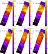 |
Fig. B.1 Spatial distribution of the six 12.7 µm AIB subcomponents, introduced in Sect. 5.4. |
| In the text | |
|
Fig. B.2 Spatial distribution of the six 12.0 µm AIB subcomponents, introduced in Sect. 5.5.1. |
| In the text | |
|
Fig. C.1 The heat map of pairwise correlation coefficients R of the surface brightnesses of AIBs with SNR > 3 from the PDR (i.e., excluding the H II region) for absolute surface brightnesses (top) and for surface brightnesses normalized to the 11.207 µm surface brightnesses (bottom). |
| In the text | |
|
Fig. C.2 Correlations of 10–15 µm AIBs with the 11.2 µm AIB surface brightnesses. The correlation coefficient, R, for the variables excluding and including the points from the H II region (black), are listed in red and black, respectively. The data points are colored according to regions in the mosaic where those pixels are located, per the color bar. |
| In the text | |
|
Fig. C.3 Correlations of the 12.805 and 12.96 µm surface brightnesses with the 11.207 µm surface brightnesses, normalized to the 11.0 µm surface brightnesses. The correlation coefficient, R, for the variables excluding and including the points from the H II region are listed in red and black, respectively. The data points are colored according to regions in the mosaic where those pixels are located, per the color bar at the bottom. |
| In the text | |
|
Fig. D.1 Spatial distribution of the PCs from round 1. |
| In the text | |
|
Fig. D.2 Biplots for the PCA round 1. Biplots show the projection of the standardized input variables on to the PCi axes. |
| In the text | |
|
Fig. D.3 Selected correlation plots for the PCA round 1. |
| In the text | |
|
Fig. D.4 Spatial maps for the PCs from PCA round 2. |
| In the text | |
|
Fig. D.5 Biplots for the PCA round 2. |
| In the text | |
|
Fig. D.6 Selected correlation plots for the PCA round 2. |
| In the text | |
|
Fig. D.7 Spatial maps for the PCs from PCA round 3. |
| In the text | |
|
Fig. D.8 Biplots for the PCA round 3. |
| In the text | |
|
Fig. D.9 Spatial distribution of the PCs from round 4. |
| In the text | |
|
Fig. D.10 Biplots for the PCA round 4. The bottom panel shows the PC1 vs. PC2 biplot when the broad 10–15 µm plateau (Fig. 3) is included. Biplots show the projection of the standardized input variables on to the PCi axes. |
| In the text | |
|
Fig. E.1 Spatial distribution of the surface brightness [W m−2 sr−1] of the 11.25 µm AIB, the 11.25/11.207 µm and 11.25/11.2 µm surface brightness ratios, the O I 1.317 µm fluorescence line [erg cm−2 s−1 sr−1] from Peeters et al. (2024), and the H2 0-0 S(3) line [W m−2 sr−1] at 9.664 µm from Sidhu et al. (in prep.). The black contours in the top right panel correspond to I11.25 = 1.25 × 10⁻⁵ W m−2 sr−1. In the top middle and right panels, the white and teal contours trace peak emission for the 11.0 µm and the 11.2 µm band, respectively, and the black contour corresponds to a 11.25/11.207 ratio of 0.8. In the bottom left panel, the dashed black line represents the “secondary ridge” discussed in the text. θ1 Ori C is located toward the top right of each map (see Fig. 2). In each map the range of the corresponding color bar is set between 0.5% and 99.5% percentile level for the data. The zero pixels, and in the maps based on the MIRI FOV, the edge pixels, and pixels covering the two proplyds, indicated by the black circles, are masked out. The rectangular apertures of the template spectra for the H II region, atomic PDR, DF 1, DF 2, and DF 3, from top to bottom, are shown in white and the solid white lines delineate the IF and the three DFs, DF 1, DF 2 and DF 3. |
| In the text | |
|
Fig. E.2 Illustration of the 11.2 µm profiles normalized to their peak specific surface brightnesses near the IF. Top: profiles, in groups of three, of the pixels that are marked by ⋆ symbols on the 11.25 µm map in Fig. E.1. Bottom: profiles from a pixel marked by a × symbol in purple near the IF and a pixel marked by a × symbol in black DF 2 in the 11.25 µm map in Fig. E.1. |
| In the text | |
|
Fig. F.1 Correlations plots of the 11.0, 11.2, 11.207, and 11.25 µm surface brightnesses in units of W m−2 sr−1. The correlation coefficient “R” for the variables excluding (including) the points from the H II region (black), are listed in red (black). The colored star symbols represent the five template spectra from the PDR (H II region: black, atomic PDR: blue; DF 1: purple; DF 2: orange; and DF 3: pink). Only surface brightnesses with SNR > 3 from every other spaxel are considered. The data points are colored according to regions in the mosaic where those pixels are located (fifth panel): black (H II region), blue (atomic PDR), teal (west IF), purple (DF 1), yellow (region between DF 1 and DF 2), orange (DF 2), light brown (region west of DF 2), brown (region between DF 2 and DF 3), pink (DF 3) and light purple (region beyond DF 3). The contours highlighting DF 2 and DF 3 are identified through enhanced emission of H2 0-0 S(3) in these DFs. The red circular regions on the color-region map (fifth panel) correspond to the proplyds, as these pixels have been masked in our data analysis. |
| In the text | |
|
Fig. F.2 Noteworthy correlations for the 12.0 µm AIB and its components. The correlation coefficient, R, for the variables excluding (including) the points from the H II region (black), are listed in red (black). The data points are colored according to regions in the mosaic, per the color bar at the bottom. |
| In the text | |
|
Fig. F.3 Correlations of the 12.0-G1 (11.90 µm) subcomponent with the 12.01 and 12.02 components. The correlation coefficient, R, for the variables excluding (including) the points from the H II region (black), are listed in red (black). The data points are colored according to regions in the mosaic, per the color bar at the bottom. |
| In the text | |
|
Fig. F.4 Correlation plots for the 12.805 µm and 12.96 µm components of the 12.7 µm AIB. The correlation coefficient, R, for the variables excluding (including) the points from the H II region (black), are listed in red (black). The data points are colored according to regions in the mosaic, per the color bar at the bottom. |
| In the text | |
|
Fig. F.5 Correlation plots for the 13.5, 12.0, and 14.2 µm bands normalized to the 11.207 µm AIB. The correlation coefficient, R, for the variables excluding (including) the points from the H II region (black), are listed in red (black). The data points are colored according to regions in the mosaic, per the color bar at the bottom. |
| In the text | |
Current usage metrics show cumulative count of Article Views (full-text article views including HTML views, PDF and ePub downloads, according to the available data) and Abstracts Views on Vision4Press platform.
Data correspond to usage on the plateform after 2015. The current usage metrics is available 48-96 hours after online publication and is updated daily on week days.
Initial download of the metrics may take a while.