| Issue |
A&A
Volume 685, May 2024
|
|
|---|---|---|
| Article Number | A75 | |
| Number of page(s) | 22 | |
| Section | Numerical methods and codes | |
| DOI | https://doi.org/10.1051/0004-6361/202346662 | |
| Published online | 14 May 2024 | |
PDRs4All
IV. An embarrassment of riches: Aromatic infrared bands in the Orion Bar★
1
Department of Physics & Astronomy, The University of Western Ontario,
London
ON
N6A 3K7,
Canada
e-mail: This email address is being protected from spambots. You need JavaScript enabled to view it.
2
Institute for Earth and Space Exploration, The University of Western Ontario,
London
ON
N6A 3K7,
Canada
3
Carl Sagan Center, SETI Institute,
339 Bernardo Avenue, Suite 200,
Mountain View,
CA
94043,
USA
4
Leiden Observatory, Leiden University,
PO Box 9513,
2300 RA
Leiden,
The Netherlands
5
Astronomy Department, University of Maryland,
College Park,
MD
20742,
USA
6
Institut de Recherche en Astrophysique et Planétologie, Université Toulouse III – Paul Sabatier, CNRS, CNES,
9 Av. du colonel Roche,
31028
Toulouse Cedex 04,
France
7
Institut d’Astrophysique Spatiale, Université Paris-Saclay, CNRS,
Bâtiment 121,
91405
Orsay Cedex,
France
8
Department of Astronomy, University of Michigan,
1085 South University Avenue,
Ann Arbor,
MI
48109,
USA
9
Space Telescope Science Institute,
3700 San Martin Drive,
Baltimore,
MD
21218,
USA
10
ACRI-ST, Centre d’Etudes et de Recherche de Grasse (CERGA),
10 Av. Nicolas Copernic,
06130
Grasse,
France
11
INCLASS Common Laboratory,
10 Av. Nicolas Copernic,
06130
Grasse,
France
12
NASA Ames Research Center,
MS 245-6,
Moffett Field,
CA
94035-1000,
USA
13
LERMA, Observatoire de Paris, PSL Research University, CNRS, Sorbonne Université,
92190
Meudon,
France
14
Instituto de Física Fundamental (CSIC),
Calle Serrano 121-123,
28006
Madrid,
Spain
15
Institut des Sciences Moléculaires d’Orsay, CNRS, Université Paris-Saclay,
Bâtiment 520,
91405
Orsay Cedex,
France
16
UK Astronomy Technology Centre, Royal Observatory Edinburgh,
Blackford Hill,
Edinburgh
EH9 3HJ,
UK
17
Observatorio Astronómico Nacional (OAN,IGN),
Alfonso XII, 3,
28014
Madrid,
Spain
18
Sterrenkundig Observatorium, Universiteit Gent,
Krijgslaan 281/S9,
9000
Gent,
Belgium
19
KU Leuven Quantum Solid State Physics (QSP),
Celestijnenlaan 200d –
PO Box 2414,
3001
Leuven,
Belgium
20
Institut de Planétologie et d’Astrophysique de Grenoble (IPAG), Université Grenoble Alpes, CNRS,
38000
Grenoble,
France
21
Institut de Radioastronomie Millimétrique (IRAM),
300 rue de la Piscine,
38406
Saint-Martin-d’Hères,
France
22
I. Physikalisches Institut der Universität zu Köln,
Zülpicher Straße 77,
50937
Köln,
Germany
23
Department of Astronomy, Graduate School of Science, The University of Tokyo,
7-3-1 Bunkyo-ku,
Tokyo
113-0033,
Japan
24
Department of Physics, Faculty of Science and Engineering, Meisei University,
2-1-1 Hodokubo, Hino,
Tokyo
191-8506,
Japan
25
Johns Hopkins University,
3400 N. Charles Street,
Baltimore,
MD
21218,
USA
26
Physikalischer Verein – Gesellschaft für Bildung und Wissenschaft,
Robert-Mayer-Straße 2,
60325
Frankfurt am Main,
Germany
27
Institut für Angewandte Physik. Goethe-Universität Frankfurt,
Max-von-Laue-Str. 1,
60438
Frankfurt am Main,
Germany
28
Department of Space, Earth and Environment, Chalmers University of Technology,
Onsala Space Observatory,
439 92
Onsala,
Sweden
29
Instituto de Astrofísica e Ciências do Espaço,
Tapada da Ajuda, Edifício Leste, 2° Piso,
1349-018
Lisboa,
Portugal
30
Instituto de Física e Química, Universidade Federal de Itajubá,
Av. BPS 1303, Pinheirinho,
37500-903,
Itajubá,
MG,
Brazil
31
Bay Area Environmental Research Institute,
Moffett Field,
CA
94035,
USA
32
Australian Synchrotron, Australian Nuclear Science and Technology Organisation (ANSTO),
800 Blackburn Rd, Clayton, Victoria 3168,
Melbourne,
Australia
33
INAF – Osservatorio Astrofisico di Catania,
Via Santa Sofia 78,
95123
Catania,
Italy
34
Laboratoire de Physique de l’École Normale Supérieure, ENS, Université PSL, CNRS, Sorbonne Université, Université de Paris,
75005
Paris,
France
35
Laboratory for Atmospheric and Space Physics, University of Colorado,
Boulder,
CO
80303,
USA
36
Department of Chemistry, University of Colorado,
Boulder,
CO
80309,
USA
37
Institute for Modeling Plasma, Atmospheres, and Cosmic Dust (IMPACT), University of Colorado,
Boulder,
CO
80303,
USA
38
Faculty of Aerospace Engineering, Delft University of Technology,
Kluyverweg 1,
2629
HS Delft,
The Netherlands
39
FELIX Laboratory, Institute for Molecules and Materials, Radboud University,
Toernooiveld 7,
6525 ED
Nijmegen,
The Netherlands
40
School of Physics, University of Hyderabad,
Hyderabad,
Telangana
500046,
India
41
Department of Earth, Environment, and Physics Worcester State University,
486 Chandler St,
Worcester,
MA
01602,
USA
42
Anton Pannekoek Institute for Astronomy (API), University of Amsterdam,
Science Park 904,
1098 XH
Amsterdam,
The Netherlands
43
Delft University of Technology, Delft,
Mekelweg 5,
2628 CD
Delft,
The Netherlands
44
Laboratoire de Physique des deux infinis Irène Joliot-Curie, Université Paris-Saclay, CNRS/IN2P3,
Bâtiment 104,
91405
Orsay Cedex,
France
45
Department of Chemistry, GITAM school of Science, GITAM Deemed to be University,
NH 207, Nagadenehalli, Doddaballapur taluk,
Bengaluru –
561203,
Karnataka,
India
46
Institut de Physique de Rennes, UMR CNRS 6251,
Université de Rennes 1, Campus de Beaulieu,
35042
Rennes Cedex,
France
47
Department of Chemistry, The University of British Columbia, Vancouver,
2036 Main Mall,
Vancouver,
BC
V6T 1Z1,
Canada
48
National Radio Astronomy Observatory (NRAO),
520 Edgemont Road,
Charlottesville,
VA
22903,
USA
49
European Space Astronomy Centre (ESAC/ESA),
Villanueva de la Cañada,
28692
Madrid,
Spain
50
Observatoire de Paris, PSL University, Sorbonne Université, LERMA,
75014
Paris,
France
51
Harvard-Smithsonian Center for Astrophysics,
60 Garden Street,
Cambridge
MA
02138,
USA
52
Sorbonne Université, CNRS, UMR 7095, Institut d’Astrophysique de Paris,
98bis bd Arago,
75014
Paris,
France
53
Institut Universitaire de France, Ministère de l’Enseignement Supérieur et de la Recherche,
1 rue Descartes,
75231
Paris Cedex 05,
France
54
Department of Physics and Astronomy, Rice University,
Houston
TX,
77005-1892,
USA
55
Yunnan Observatories, Chinese Academy of Sciences,
396 Yangfangwang, Guandu District,
Kunming
650216,
PR China
56
Chinese Academy of Sciences South America Center for Astronomy, National Astronomical Observatories, CAS,
Beijing
100101,
PR China
57
Departments of Chemistry and Astronomy, University of Virginia,
Charlottesville,
Virginia
22904,
USA
58
InterCat and Dept. Physics and Astron., Aarhus University,
Ny Munkegade 120,
8000
Aarhus C,
Denmark
59
Laboratory Astrophysics Group of the Max Planck Institute for Astronomy at the Friedrich Schiller University Jena, Institute of Solid State Physics,
Helmholtzweg 3,
07743
Jena,
Germany
60
Instituto de Astronomia, Geofísica e Ciências Atmosféricas, Universidade de São Paulo,
05509-090
São Paulo,
SP,
Brazil
61
Department of Physics and Astronomy, San José State University,
San Jose,
CA
95192,
USA
62
Institut de Ciencies de l’Espai (ICE, CSIC),
Can Magrans, s/n,
08193
Bellaterra,
Barcelona,
Spain
63
ICREA,
Pg. Lluìs Companys 23,
08010
Barcelona,
Spain
64
Institut d’Estudis Espacials de Catalunya (IEEC),
08034
Barcelona,
Spain
65
European Space Agency, Space Telescope Science Institute,
3700 San Martin Drive,
Baltimore
MD
21218,
USA
66
Institute of Astronomy, Russian Academy of Sciences,
119017,
Pyatnitskaya str. 48,
Moscow,
Russia
67
Department of Earth, Ocean, & Atmospheric Sciences, University of British Columbia,
British Columbia
V6T 1Z4,
Canada
68
Telespazio UK for ESA, ESAC,
28692 Villanueva de la Cañada,
Madrid,
Spain
69
IPAC, California Institute of Technology,
Pasadena,
CA,
USA
70
Department of Physics and Astronomy, University of Missouri,
701 S College Ave,
Columbia,
MO
65211,
USA
71
Max Planck Institute for Astronomy,
Königstuhl 17,
69117
Heidelberg,
Germany
72
Chemical Sciences Division, Lawrence Berkeley National Laboratory,
Berkeley,
CA,
USA
73
Kenneth S. Pitzer Center for Theoretical Chemistry, Department of Chemistry,
420 Latimer Hall, University of California,
Berkeley,
CA
94720-1460,
USA
74
AIM, CEA, CNRS, Université Paris-Saclay, Université Paris Diderot,
Sorbonne Paris Cité,
91191
Gif-sur-Yvette,
France
75
Institut des Sciences Moléculaires, CNRS, Université de Bordeaux,
33405
Talence,
France
76
Department of Chemistry, Massachusetts Institute of Technology,
Cambridge,
MA
02139,
USA
77
Instituto de Ciencia de Materiales de Madrid (CSIC),
Sor Juana Ines de la Cruz 3,
28049,
Madrid,
Spain
78
Department of Physics,
PO Box 64,
00014
University of Helsinki,
Helsinki,
Finland
79
Steward Observatory, University of Arizona,
Tucson,
AZ
85721-0065,
USA
80
BoldlyGo Institute,
31 W 34TH ST FL 7 STE 7159,
New York,
NY
10001,
USA
81
Department of Physics, College of Science, United Arab Emirates University (UAEU),
Al-Ain
15551,
UAE
82
National Astronomical Observatory of Japan, National Institutes of Natural Science,
2-21-1 Osawa, Mitaka,
Tokyo
181-8588,
Japan
83
Sorbonne Université, CNRS, UMR 7095, Institut d’Astrophysique de Paris,
98bis bd Arago,
75014
Paris,
France
84
California Institute of Technology, IPAC,
770, S. Wilson Ave.,
Pasadena,
CA
91125,
USA
85
Department of Physics, Institute of Science, Banaras Hindu University,
Varanasi
221005,
India
86
University of Central Florida,
Orlando,
FL
32765,
USA
87
Van’t Hoff Institute for Molecular Sciences, University of Amsterdam,
PO Box 94157,
1090 GD,
Amsterdam,
The Netherlands
88
Laboratoire de Chimie et Physique Quantiques LCPQ/FERMI, UMR5626, Université de Toulouse (UPS) and CNRS,
Toulouse,
France
89
Laboratory Astrophysics Group of the Max Planck Institute for Astronomy at the Friedrich Schiller University Jena, Institute of Solid State Physics,
Helmholtzweg 3,
07743
Jena,
Germany
90
Instituto de Matemática, Estatística e Física, Universidade Federal do Rio Grande,
96201-900
Rio Grande,
RS,
Brazil
91
Center for Astrophysics and Space Sciences, Department of Physics, University of California,
San Diego, 9500 Gilman Drive,
La Jolla,
CA
92093,
USA
92
School of Chemistry, The University of Nottingham,
University Park,
Nottingham
NG7 2RD,
UK
93
Astronomy Department, Ohio State University,
Columbus,
OH
43210,
USA
94
Space Science Institute,
4765 Walnut St., R203,
Boulder,
CO
80301,
USA
95
Department of Physics, Stockholm University,
10691
Stockholm,
Sweden
96
Department of Physics, Texas State University,
San Marcos,
TX
78666,
USA
97
School of Physics and Astronomy, Sun Yat-sen University,
2 Da Xue Road, Tangjia,
Zhuhai
519000,
Guangdong Province,
PR China
98
Star and Planet Formation Laboratory, RIKEN Cluster for Pioneering Research,
Hirosawa 2-1, Wako,
Saitama
351-0198,
Japan
99
Institute of Deep Space Sciences, Deep Space Exploration Laboratory,
Hefei
230026,
PR China
Received:
14
April
2023
Accepted:
1
August
2023
Abstract
Context. Mid-infrared observations of photodissociation regions (PDRs) are dominated by strong emission features called aromatic infrared bands (AIBs). The most prominent AIBs are found at 3.3, 6.2, 7.7, 8.6, and 11.2 µm. The most sensitive, highest-resolution infrared spectral imaging data ever taken of the prototypical PDR, the Orion Bar, have been captured by JWST. These high-quality data allow for an unprecedentedly detailed view of AIBs.
Aims. We provide an inventory of the AIBs found in the Orion Bar, along with mid-IR template spectra from five distinct regions in the Bar: the molecular PDR (i.e. the three H2 dissociation fronts), the atomic PDR, and the H II region.
Methods. We used JWST NIRSpec IFU and MIRI MRS observations of the Orion Bar from the JWST Early Release Science Program, PDRs4All (ID: 1288). We extracted five template spectra to represent the morphology and environment of the Orion Bar PDR. We investigated and characterised the AIBs in these template spectra. We describe the variations among them here.
Results. The superb sensitivity and the spectral and spatial resolution of these JWST observations reveal many details of the AIB emission and enable an improved characterization of their detailed profile shapes and sub-components. The Orion Bar spectra are dominated by the well-known AIBs at 3.3, 6.2, 7.7, 8.6, 11.2, and 12.7 µm with well-defined profiles. In addition, the spectra display a wealth of weaker features and sub-components. The widths of many AIBs show clear and systematic variations, being narrowest in the atomic PDR template, but showing a clear broadening in the H II region template while the broadest bands are found in the three dissociation front templates. In addition, the relative strengths of AIB (sub-)components vary among the template spectra as well. All AIB profiles are characteristic of class A sources as designated by Peeters (2022, A&A, 390, 1089), except for the 11.2 µm AIB profile deep in the molecular zone, which belongs to class B11.2. Furthermore, the observations show that the sub-components that contribute to the 5.75, 7.7, and 11.2 µm AIBs become much weaker in the PDR surface layers. We attribute this to the presence of small, more labile carriers in the deeper PDR layers that are photolysed away in the harsh radiation field near the surface. The 3.3/11.2 AIB intensity ratio decreases by about 40% between the dissociation fronts and the H II region, indicating a shift in the polycyclic aromatic hydrocarbon (PAH) size distribution to larger PAHs in the PDR surface layers, also likely due to the effects of photochemistry. The observed broadening of the bands in the molecular PDR is consistent with an enhanced importance of smaller PAHs since smaller PAHs attain a higher internal excitation energy at a fixed photon energy.
Conclusions. Spectral-imaging observations of the Orion Bar using JWST yield key insights into the photochemical evolution of PAHs, such as the evolution responsible for the shift of 11.2 µm AIB emission from class B11.2 in the molecular PDR to class A11.2 in the PDR surface layers. This photochemical evolution is driven by the increased importance of FUV processing in the PDR surface layers, resulting in a “weeding out” of the weakest links of the PAH family in these layers. For now, these JWST observations are consistent with a model in which the underlying PAH family is composed of a few species: the so-called ‘grandPAHs’.
Key words: astrochemistry / infrared: ISM / ISM: molecules / ISM: individual objects: Orion Bar / photon-dominated region (PDR) / techniques: spectroscopic
The 5 template spectra are available at the CDS via anonymous ftp to cdsarc.cds.unistra.fr (130.79.128.5) or via https://cdsarc.cds.unistra.fr/viz-bin/cat/J/A+A/685/A75
Tim Lee sadly passed away on Nov. 3, 2022.
© The Authors 2024
 Open Access article, published by EDP Sciences, under the terms of the Creative Commons Attribution License (https://creativecommons.org/licenses/by/4.0), which permits unrestricted use, distribution, and reproduction in any medium, provided the original work is properly cited.
This article is published in open access under the Subscribe to Open model. This email address is being protected from spambots. You need JavaScript enabled to view it. to support open access publication.
1 Introduction
A major component of the infrared (IR) emission near star-forming regions in the Universe consists of a set of broad emission features at 3.3, 6.2, 7.7, 8.6, 11.2, and 12.7 µm (e.g. Tielens 2008, and references therein). These mid-IR emission features, referred to as aromatic infrared bands (AIBs), are generally attributed to vibrational emission from polycyclic aromatic hydrocarbons and related species upon absorption of interstellar far-ultraviolet (FUV; 6–13.6 eV) photons (Léger & Puget 1984; Allamandola et al. 1985). The AIB spectrum is very rich and consists of the main bands listed above and a plethora of weaker emission features. Moreover, many AIBs are in fact blends of strong and weak bands (e.g. Peeters et al. 2004a). The AIB emission is known to vary from source to source and spatially within extended sources in terms of the profile and relative intensities of the features (e.g. Joblin et al. 1996; Hony et al. 2001; Berné et al. 2007; Sandstrom et al. 2010; Boersma et al. 2012; Candian et al. 2012; Stock & Peeters 2017; Peeters et al. 2017). These remarkably widespread emission features have been described in many diverse astronomical sources, including protoplanetary disks (e.g. Meeus et al. 2001; Vicente et al. 2013), H II regions (e.g. Bregman 1989; Peeters et al. 2002b), reflection nebulae (e.g. Peeters et al. 2002a; Werner et al. 2004), planetary nebulae (e.g. Gillett et al. 1973; Bregman 1989; Beintema et al. 1996), the interstellar medium (ISM) of galaxies ranging from the Milky Way (Boulanger et al. 1996), the Magellanic Clouds (e.g. Vermeij et al. 2002; Sandstrom et al. 2010), starburst galaxies, luminous and ultra-luminous IR galaxies, and high-redshift galaxies (e.g. Genzel et al. 1998; Lutz et al. 1998; Peeters et al. 2004b; Yan et al. 2005; Galliano et al. 2008), as well as in the harsh environments of galactic nuclei (e.g. Smith et al. 2007; Esquej et al. 2014; Jensen et al. 2017).
A useful observational proxy for studying AIBs is the spectroscopic classification scheme devised by Peeters et al. (2002a) which classifies each individual AIBs based on their profile shapes and precise peak positions (classes A, B, and C). While the AIBs observed in a given source generally belong to the same class, this is not always the case. In particular, the classes in the 6 to 9 µm region do not always correspond to those of the 3.3 and 11.2 AIBs (van Diedenhoven et al. 2004). Class A sources are the most common – they exhibit the “classical” AIBs, with a 6.2 µm AIB that peaks between 6.19 and 6.23 µm, a 7.7 µm complex in which the 7.6 µm sub-peak is stronger than the 7.8 µm sub-peak, and the 8.6 µm feature peaks at 8.6 µm. Class B sources can be slightly redshifted compared to class A, while at the same time the 7.7 µm complex peaks between 7.8 and 8 µm. Class C sources show a very broad emission band peaking near 8.2 µm, and typically do not exhibit the 6.2 or 7.7 µm AIBs.
These three classes were found to show a strong correlation with the type of object considered. The most common AIB spectrum, class A, is identified in the spectra of photodissociation regions (PDRs), HII regions, reflection nebulae, the ISM, and galaxies. The most widely used template for class A sources has been the spectrum of the Orion Bar (Peeters et al. 2002a; van Diedenhoven et al. 2004). Class B sources are isolated Herbig Ae/Be stars and a few evolved stars; in fact, evolved star spectra can belong to either of the classes. Class C sources include post-AGB and Herbig Ae/Be stars, as well as a few T Tauri disks (Peeters et al. 2002a; Bouwman et al. 2008; Shannon & Boersma 2019). More recent work has developed analogous classification schemes for other AIBs and has included a new class D (e.g. van Diedenhoven et al. 2004; Sloan et al. 2014; Matsuura et al. 2014).
Observed variations in AIBs reflect changes in the molecular properties of the species responsible for the AIB emission (charge, size, and molecular structure; e.g. Joblin et al. 1996; Berné et al. 2007; Pilleri et al. 2012; Boersma et al. 2013; Candian & Sarre 2015; Peeters et al. 2017; Robertson 1986; Dartois et al. 2004; Pino et al. 2008; Godard et al. 2011; Jones et al. 2013), which are set by the local physical conditions (including FUV radiation field strength, G0, gas temperature, and density, n(H); e.g. Bakes et al. 2001; Galliano et al. 2008; Pilleri et al. 2012, 2015; Stock et al. 2016; Schirmer et al. 2020, 2022; Sidhu et al. 2022; Knight et al. 2022b; Murga et al. 2022). The observed variability in AIB emission thus implies that the population responsible for their emission is not static, but undergoes photochemical evolution.
Observations using space-based IR observatories – in particular the Short-Wavelength Spectrometer (SWS; de Graauw et al. 1996) on board the Infrared Space Observatory (ISO; Kessler et al. 1996) and the Infrared Spectrograph (IRS; Houck et al. 2004) on board the Spitzer Space Telescope (Werner et al. 2004) – have revealed the richness of AIBs (for a review see e.g. Peeters et al. 2004a; Tielens 2008). However, obtaining a full understanding of the photochemical evolution underlying AIBs has been limited by insufficient spatial and spectral resolution (e.g. Spitzer-IRS) or by limited sensitivity and spatial resolution (e.g. ISO/SWS) of these IR facilities.
JWST is set to unravel the observed complexity of AIBs, as it offers access to the full wavelength range of importance for AIB studies at medium spectral resolution and at unprecedented spatial resolution and sensitivity. JWST is able to resolve, for the first time, where and how the photochemical evolution of polycyclic aromatic related species, the carriers of AIBs, occurs while providing a detailed view of the resulting AIB spectral signatures. The PDRs4All JWST Early Release Science Program observed the prototypical highly irradiated PDR, the Orion Bar (Berné et al. 2022; Habart et al. 2023; Peeters et al. 2024). The Orion Bar PDR has a G0 which varies with position from about 1 × 10⁴ to 4 × 10⁴ Habings (e.g. Marconi et al. 1998; Peeters et al. 2024) and it has a gas density which varies from of a few 104 cm−3 in the atomic PDR to ~106 cm−3 in the molecular region (e.g. Parmar et al. 1991; Tauber et al. 1994; Young Owl et al. 2000; Bernard-Salas et al. 2012; Goicoechea et al. 2016; Joblin et al. 2018; Habart et al. 2023). Given the proximity of Orion (414 pc; Menten et al. 2007), the PDRs4All dataset takes full advantage of JWST’s spatial resolution to showcase the AIB emission in unprecedented detail.
In this paper, we present five MIRI-MRS template spectra representing key regions of the Orion Bar PDR. Combined with corresponding JWST NIRSpec-IFU template spectra (Peeters et al. 2024), we present an updated inventory and characterization of the AIB emission in this important reference source. We describe the observations, data reduction, and the determination of the underlying continuum in our template spectra in Sect. 2. In Sect. 3, we give a detailed account of the observed AIB bands and sub-components along with their vibrational assignments. We compare our findings with previous works and discuss the AIB profiles and the AIB variability in the Orion Bar in Sect. 4. Finally, we summarize our results and narrate a picture of the origins and evolution of the AIB emission in Sect. 5.
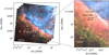 |
Fig. 1 PDRs4All MIRI MRS and NIRSpec footprints (dashed and solid white boundaries, respectively), and spectral extraction apertures (black boxes in the right panel) on top of a composite NIRCam image of the Orion Bar (data from Habart et al. 2023). DF 1, DF 2, and DF 3 are H2 dissociation fronts as designated in Habart et al. (2023). Red, green, and blue are encoded as F335M (AIB), F470N-F480M (H2 emission), and F187N (Paschen α), respectively. |
2 Data and data processing
2.1 MIRI-MRS observations and data reduction
On 30 January 2023, JWST observed the Orion Bar PDR with the Mid-Infrared Instrument (MIRI) in medium resolution spectroscopy (MRS) mode (Wells et al. 2015; Argyriou et al. 2023) as part of the PDRs4All Early Release Science program (Berné et al. 2022). We obtained a 1 × 9 pointing mosaic in all four MRS channels (channels 1, 2, 3, and 4), and all three sub-bands within each channel (short, medium, and long). We applied a 4-point dither optimised for extended sources and use the FASTR1 readout pattern adapted for bright sources. We integrated for 521.7 s using 47 groups per integration and 4 integrations. The resulting datacube thus spans the full MRS wavelength range (4.90–27.90 µm) with a spectral resolution ranging from R ~ 3700 in channel 1 to ~ 1700 in channel 4 and a spatial resolution of 0.207″ at short wavelengths to 0.803″ at long wavelengths, corresponding to 86 and 332 AU, respectively at the distance of the Orion Nebula.
The mosaic was positioned to overlap the PDRs4All JWST Near Infrared Spectrograph (NIRSpec) IFU (Böker et al. 2022) observations of the Orion Bar (Peeters et al. 2024; Fig. 1). Given the different fields of view of the MRS channels (~3″ in channel 1 to ~7″ in channel 4), the spatial footprint with full wavelength coverage is limited by the field of view (FOV) of channel 1. The footprint shown in Fig. 1 represents the area with full MRS wavelength coverage, noting that the MRS data in channels 2–4 exist beyond the area shown, but we choose to use only the sub-set of data with full wavelength coverage. The NIRSpec IFU and MIRI MRS datasets combined provide a perpendicular cross-section of the Orion Bar from the H II region to the molecular zone at very high spatial and spectral resolution from 0.97 to 27.9 µm.
We reduced the MIRI-MRS data using version 1.9.5. dev10+g04688a77 of the JWST pipeline1, and JWST Calibration Reference Data System2 (CRDS) context 1041. We ran the JWST pipeline with default parameters except the following. The master background subtraction, outlier detection, fringe-and residual-fringe correction steps were all turned on. Cubes were built using the drizzle algorithm. The pipeline combined all pointings for each sub-band, resulting in 12 cubes (4 channels of 3 sub-bands each) covering the entire field of view.
We stitched the 12 sub-band cubes into a single cube by reprojecting all of the cubes onto a common spatial grid using channel 1 short as a reference. We then scaled the spectra to match in flux where they overlap using channel 2 long as the reference. This stitching algorithm is part of the “Haute Couture” algorithm described in Canin et al. (in prep.).
While the pipeline and reference files produce high-quality data products, a few artefacts still remain in the data. The most important artifacts for our analysis are fringes and flux calibration that are not yet finalised (see Appendix B). Neither of these artefacts have a strong impact on our results, as discussed in Appendix B, although we do limit our analysis to wavelengths ≤15 µm due to the presence of artefacts beyond this range.
2.2 Extracting template spectra from key regions
We extracted MIRI template spectra using the same extraction apertures as Peeters et al. (2024)3. These apertures are selected to represent the key physical zones of the Orion Bar PDR: the H II region, the atomic PDR, and the three bright H I/H2 dissociation fronts (DF 1, DF 2, and DF 3) corresponding to three molecular hydrogen (H2) filaments that were identified in the NIRSpec FOV (Fig. 1). We emphasize that the remaining areas in the MRS spectral map will be analysed at a later time. We note that the AIB emission detected in the H II region template originates from the background PDR. Combined with the NIR-Spec templates of Peeters et al. (2024), these spectra capture all of the AIB emission in each of the five regions. In this paper, we focus on the inventory and characterization of the AIBs found in these template spectra. We refer to Peeters et al. (2024) and Van De Putte et al. (2023) for the inventories of the gas lines from atoms and small molecules extracted from NIRSpec and MIRI MRS data, respectively. For a detailed description of the Orion Bar PDR morphology as seen by JWST we refer to Habart et al. (2023) and to Peeters et al. (2024).
2.3 Measuring the underlying continuum
The AIB emission is perched on top of the continuum emission from stochastically heated very small grains (e.g. Smith et al. 2007). Different spectral decomposition methods have deduced additional emission components referred to as: 1) emission from evaporating very small grains (based on the blind signal separation method; Berné et al. 2007; Pilleri et al. 2012; Foschino et al. 2019) and 2) plateau emission due to large PAHs, PAH clusters and nanoparticles (Bregman et al. 1989; Roche et al. 1989; Peeters et al. 2012, 2017; Boersma et al. 2014; Sloan et al. 2014).
In order to identify and characterize AIBs, we subtracted estimates of the continuum emission in each template spectrum. We computed a linear continuum for NIRSpec and a spline continuum anchored at selected wavelengths for MIRI data. Furthermore, we adopted the same anchor points for all five templates. While our measurements of the full-width at half-maximum (FWHM) of AIBs (see Table 1) do depend on the selected continuum, we note that our main goal – to catalog AIBs and their sub-components qualitatively – does not require highly precise estimates of the continuum.
The FWHM4 of each AIB complex was measured by normalizing the continuum-subtracted template spectrum by the peak intensity of the AIB and then calculating the FWHM of the entire AIB complex, that is, without taking into consideration blends, components, and/or sub-components that make up the AIB complex. The measured FWHM strongly depends on the estimated continuum emission; however, this does not impact qualitative trends in FWHM from template to template. The integrated flux of each AIB was computed from the continuum-subtracted spectra. We refer to Peeters et al. (2024) for details on how the 3.3 and 3.4 µm AIB fluxes were measured.
FWHM of AIBs and AIB complexes measured from five template spectra extracted from NIRSpec-IFU (first row) and MIRI-MRS (rows 2–6) observations of the Orion Bar.
3 AIB characteristics and assignments
The superb quality of the Orion Bar observations combined with the increased spectral resolution compared to prior IR space observations reveals an ever-better characterization of the AIBs in terms of sub-components, multiple components making up a “single” band, and the precise shapes of the band profiles (see Fig. 2 for an overview and Figs. 3 and 4 for zoom-ins of selected AIBs in the five template spectra).
We offer a detailed description of the spectral characteristics of the AIB emission as seen by JWST as well as current vibrational assignments in Sects. 3.1 to 3.6. The detailed AIB inventory is listed in Table A.1. We note that we consider all spectrally resolved emission features to be candidate AIBs. To assess whether a candidate AIB is real or an artefact, we compare the template spectra in the location of the candidate AIB to the spectrum of the calibration standard star 10 Lac (see Appendix B for details). Due to the very high signal-to-noise ratio (S/N), the spectra reveal an abundance of weak features, either as standalone features, or as shoulders of other bands. Occasionally these shoulders are only visible as a change in the slope along the wing of a stronger AIB and, in such cases, we estimated the central wavelength of the weak AIB visually based on the AIB profile of the main component.
Hereafter, all mentions of nominal AIBs, given in boldface in Col. 1 of Table A.1, namely 3.3, 3.4, 5.25, 5.75, 6.2, 7.7, 8.6, 11.2, 12.0, 12.7, and 13.5 µm, do not indicate the precise peak positions of these AIBs. The precise peak positions of these nominal AIBs are reported in terms of wavelength in Col. 3 of Table A.1. We note that we converted the positions in wavelength to wavenumber by rounding to the nearest integer in units of cm−1 and so the precision of the reported wavenumbers does not reflect the instrumental precision of the peak position of the AIBs.
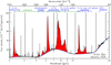 |
Fig. 2 AIB spectrum as seen by JWST using the Orion Bar atomic PDR template spectrum (Sect. 2.2) as an example. Red shaded regions indicate emission from AIBs while blue curves indicate the underlying continuum. Figure is adapted from Peeters et al. (2004a). |
3.1 The 3.2–3.5 µm (3125–2860 cm−1) range
The 3 µm spectral region is dominated by the 3.3 and 3.4 µm AIBs that peak at 3.29 and 3.4 µm, respectively. While some studies have found that the peak of the 3.3 µm AIB shifts toward longer wavelengths (van Diedenhoven et al. 2004), our measurements of the peak position of this band in each template are consistent with the nominal value of 3.29 µm. The band profiles, however, show some slight differences among the templates. The width of the 3.29 µm band varies slightly (see Table 1 and Fig. 5). The templates in order of increasing 3.29 µm band width are: atomic PDR, DF 1, H II region, DF 2, and DF 3. While the small increase in width on the red side may be attributed to underlying broad plateau emission (see Peeters et al. 2024), the blue wing broadens by ~5 cm−1 on a total band width of ~37.5 cm−1 (Table 1 and Peeters et al. 2024).
The 3.29 µm band is characteristic for the CH stretching mode in PAHs. The peak position is somewhat dependent on molecular structure, for example the number of adjacent hydrogens on a ring and steric hindrance between opposing hydrogens in so-called ‘bay’ regions. Molecular symmetry has a more important effect as it controls the number of allowed transitions and the range over which IR activity is present (Maltseva et al. 2015, 2016). For a given PAH, the initial excitation energy has a very minor influence on the peak position (Mackie et al. 2022). Earlier works have also demonstrated this minor influence (Joblin et al. 1995; Pech et al. 2002). Additionally, Tokunaga & Bernstein (2021) found that the peak position and width of the 3.3 µm feature must be fitted simultaneously as both depend on the carrier. There is also a weak dependence of peak position on the charge state, but since the CH stretch is very weak in cations (Allamandola et al. 1999; Peeters et al. 2002a), this is of no consequence. These modes are very much influenced by resonance effects with combination bands involving CC modes and CH in-plane bending modes (Mackie et al. 2015, 2016). Overall, in the emission spectra of highly excited species, the differences in peak position mentioned here will be too subtle compared to the impact of molecular symmetry when attempting to identify the carrier(s). The observed narrow width of the 3.3 µm AIB implies then emission by very symmetric PAHs (Pech et al. 2002; Ricca et al. 2012; Mackie et al. 2022).
The very weak shoulder on the blue side, namely, at ≃3.246 µm, has the same strength relative to the main feature in all template spectra, suggesting it is part of the same emission complex. Its peak wavelength may point toward the stretching mode of aromatic CH groups in bay regions or, alternatively, the effect of resonant interaction in a specific species (van Diedenhoven et al. 2004; Candian et al. 2012; Mackie et al. 2015) or aromatic CH in polyaromatic carbon clusters (Dubosq et al. 2023). In a recent analysis of the 3.3 µm AIB in the Red Rectangle, Tokunaga et al. (2022) found differences in the spectra of this source compared to earlier analyses (e.g. Tokunaga et al. 1991; Candian et al. 2012) due to the treatment of Pfund emission lines from the standard star. Candian et al. (2012) fit the 3.3 µm AIB in each spaxel of their IFU cube with two components and analysed spatial variations in the integrated intensities of these components. While issues with the standard star spectrum would affect all spectra in the cube (Tokunaga et al. 2022), spatial variations in integrated intensities should not be affected.
The AIB spectra reveal a plethora of bands longward of the 3.29 µm feature between ≃3.4 and ≃3.6 µm (Table A.1; Peeters et al. 2024; Sloan et al. 1997). As the relative strengths of these sub-components show variations from source to source and within sources (e.g. Joblin et al. 1996; Pilleri et al. 2015; Peeters et al. 2024), they are generally ascribed to different emitting groups on PAHs. Here, we note that the emission profile of the 3.4 µm band varies between the five templates, broadening to longer wavelength (Peeters et al. 2024), indicating the presence of multiple components in the main 3.4 µm band at 3.395, 3.403, and 3.424 µm. The other bands do not show such profile variations. Bands in this wavelength range are due to the CH stretching mode in aliphatic groups and assignments to methyl (CH3) groups attached to PAHs and to superhydrogenated PAHs have been proposed (Joblin et al. 1996; Bernstein et al. 1996; Maltseva et al. 2018; Buragohain et al. 2020; Pla et al. 2020). As for the aromatic CH stretching mode, the peak position is sensitive to resonances with combination bands of CC modes and CH in-plane bending modes (Mackie et al. 2018). Typically, methylated PAHs show a prominent band around 3.4 µm, but its peak position falls within a wide range, ≃0.17 µm (Maltseva et al. 2018; Buragohain et al. 2020). For hydrogenated PAHs, the main activity is at slightly longer wavelengths, ≃3.5 µm within a somewhat narrower range (≃0.05 µm). As the extra hydrogens in superhydrogenated PAHs are relatively weakly bound (1.4–1.8 eV; Bauschlicher & Ricca 2014), astronomical models imply that superhydrogenated PAHs quickly lose all these sp3 hydrogens in strongly irradiated PDRs (e.g. when G0/n(H) > 0.03; Andrews et al. 2016).
For further analysis of the AIB emission in this region, including the many weaker features listed in Table A.1, we refer to Peeters et al. (2024).
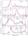 |
Fig. 3 Zoom-ins on the template spectra at wavelength regions centered on the 3.3 µm AIB (Peeters et al. 2024, top), the 6.2 µm AIB (second from top), the 7.7 µm AIB (second from bottom), and the 11.2 µm AIB (bottom). Each spectrum (on an Fν scale) is normalised by the peak surface brightness of the indicated AIB on the y-axes in each panel. The vertical tick marks indicate the positions of identified (blue) or tentative (black) AIBs and components (see Table A.1 and main text). A post-pipeline correction for residual artifacts was performed for Ch2-long (10.02–11.70 µm), Ch3-medium (13.34–15.57 µm), and Ch3-long (15.41–17.98 µm). For further details, see Appendix B. Red dashed vertical ticks indicate the wavelengths where we switch from using data from one MRS sub-band to another. Continued in Fig. 4. |
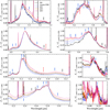 |
Fig. 4 Continued from Fig. 3. From left to right, top to bottom: zoom-ins on the template spectra normalised by the peak flux of the 5.25, 5.75 and 5.878, 6.2, 8.6, 11.2 and 12.0, 12.7, 13.5, and 14.2 µm AIBs (indicated in the y-axis label of each panel). The panels show wavelength ranges that are also shown in Fig. 3, except for the panels that are centered on the 13.5 and 14.2 µm AIBs (small panels in the lower right). These figures illustrate the overall similarity and subtle differences in AIB profiles from region to region. |
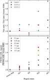 |
Fig. 5 Variation from region to region in the ratios of AIB integrated fluxes (top) and the widths of AIBs (bottom; data from Table 1). All values are normalised to those from the atomic PDR. The ordering of the regions on the x-axis is arbitrary, but was chosen so that the data roughly show an increasing trend in FWHM from left to right (Sect. 4.3). |
3.2 The 5–6 µm (1600–2000 cm−1) range
In the 5–6 µm region, previous observations have revealed two moderately weak AIB features at approximately 5.25 and 5.75 µm (Table A.1; Allamandola et al. 1989a; Boersma et al. 2009b). The 5.25 µm band (Fig. 4) consists of a broad blue shoulder centered at ~5.18 µm and extending to about 5.205 µm, followed by a sharp blue rise to a peak at 5.236 µm and a strong red wing extending to about 5.38 µm. A detailed inspection of the profiles reveals a very weak feature at ~5.30 µm superposed on the red wing. Comparing the five template spectra, we conclude that the 5.25 µm feature broadens, in particular on the red side, with the narrowest feature seen in the atomic PDR, and then increasing in width in the H II region, DF 1, DF 2, and DF 3 (Table 1 and Fig. 5). Besides the broadening, the observed profiles are very similar for the five templates, implying that the main feature consists of a single band.
Inspection of the template spectra (Fig. 4) reveals that the 5.75 µm band is a blend of three bands at 5.642, 5.699, and 5.755 µm (e.g. comparing the atomic PDR and DF 3 spectra in Fig. 4). The MIRI MRS spectra clearly exhibit a new, symmetric feature at 5.878 µm. We also report a tentative detection of two very weak features at 5.435 and 5.535 µm.
The spectra of PAHs show weak combination bands in this wavelength range generated by modes of the same type, for example, out-of-plane (OOP) modes (Boersma et al. 2009b,a). Combination bands involving in-plane modes occur at shorter wavelengths (3.8–4.4 µm) and are typically an order of magnitude weaker (Mackie et al. 2015, 2016). Combination bands involving the OOP bending modes typically result in a spectrum with two relatively simple AIBs near 5.25 and 5.75 µm. For small PAHs, the ratio of the intrinsic strength of these bands to the OOP modes increases linearly with PAH size (Lemmens et al. 2019). This ratio increases further for the larger PAHs studied in Lemmens et al. (2021). However, whether the correlation continues linearly is yet to be confirmed.
3.3 The 6.2 µm (1610 cm−1) AIB
The interstellar 6.2 µm band is one of the main AIBs. The profile peaks at 6.212 µm (1610 cm−1) and has a steep blue rise, a pronounced red wing, and a blue broad shoulder centered at ~6.07 µm. Comparing the five template spectra, we conclude that the feature broadens toward the blue side at the same time that the red wing becomes more pronounced (by about 8.2 cm−1 on a total width of ≃33.6 cm−1; Table 1). Pending confirmation, the peak position possibly varies (its value ranges from 6.2115 to 6.2161 µm). There is a distinct weaker feature at 6.024 µm (1660 cm−1) superposed on the blue shoulder. This symmetric feature has a constant width and varies in intensity independently of the main feature (see Fig. 4). This suggests that the 6.024 µm band is an independent component. We note that the observed strength variations of the 6.024 µm band do not affect the conclusion on the broadening of the blue side of the 6.2 µm band. There is a very weak feature perched on the red wing at 6.395 µm (1564 cm−1) in the template of the atomic region. It may be obscured by the stronger red wing in the other template spectra. A very subtle change in slope of the red wing may also be present near 6.5 µm in some templates (e.g. the atomic PDR).
Pure aromatic CC stretching modes fall between 6.1 and 6.5 µm. In the 6–9 µm wavelength range, the number of bands and their precise positions will depend on charge, molecular structure, size, and heterogeneity. In particular, their intrinsic strengths are very sensitive to the charge state of the species, increasing by about a factor of 10 for cations (Allamandola et al. 1999; Peeters et al. 2002a; Bauschlicher et al. 2008). Given the observed strength of the 6.2 µm band relative to the CH stretching and OOP bending modes that dominate the neutral spectra, this AIB is attributed to PAH cations (Allamandola et al. 1999). In the past, the peak position was somewhat of an enigma. In early comparisons with harmonic calculations, this band arose at too red a wavelength in PAH cations. This problem was compounded by the adoption of a redshift of 15 cm−1 to account for anharmonic effects during the emission cascade (for a summary, see Bauschlicher et al. 2009). However, model studies have revealed that anharmonicity introduces a red wing on the profile but does not lead to an appreciable redshift of the peak (Mackie et al. 2022). Recent experimental and quantum chemical studies of neutral, symmetric PAHs have shown that the mismatch between the experimental and interstellar 6.2 µm band positions is less severe than thought (Lemmens et al. 2021). Furthermore, quantum chemical studies on PAH cations have employed the cc-pVTZ basis set that better accounts for treatment of polarization in PAHs. With this basis set used in density functional theory calculations, the calculated peak position of the aromatic CC stretching mode in cations is in much better agreement with the observations (Ricca et al. 2021), but this still needs to be confirmed by experimental studies on PAH cations. The discrepancy noted in earlier studies between the peak position of the 6.2 µm AIB and the aromatic CC stretch in PAHs has prompted a number of suggestions. Specifically, incorporation of heteroatoms such as N into the ring backbone or coordination of atoms such as Si, the presence of aliphatic structures, protonated PAHs, and/or (pentagonal) defects will induce blue shifts in the peak position of this mode (Hudgins et al. 2005; Pino et al. 2008; Joalland et al. 2009; Carpentier et al. 2012; Galué 2014; Tsuge et al. 2018; Wenzel et al. 2022; Rap et al. 2022). Further studies are warranted to assess whether these suggestions are still relevant.
The observed 6.024 µm band is at too short a wavelength to be an aromatic CC stretching vibration. Rather, this position is characteristic of the C=O stretch in conjugated carbonyl groups; that is, as quinones or attached to aromatic rings (Allamandola et al. 1989b; Sarre 2019). This band has not been the focus in many quantum chemical studies. We also note that the very weak feature at 6.395 µm is likely another aromatic CC stretching mode.
3.4 The 7.7 µm (1300 cm−1) AIB complex
It has been well established that the 7.7 µm AIB is a blend of several features (Bregman 1989; Cohen et al. 1989; Peeters et al. 2002a). The JWST spectra reveal that the main component at 7.626 µm is accompanied by moderately strong bands at 7.8 and 7.85 µm. The 7.8 µm component appears narrower in DF 2 and DF 3, peaking near 7.743 µm, although this may arise due to differences in the red wing of the 7.626 µm component or this may reflect the lack of a different component at 7.775 µm present in the atomic PDR, the H II region and DF 1. In any case, given the observed variations between the templates, these bands are independent components. The 7.7 µm AIB complex as a whole broadens significantly from the atomic to the molecular region (by about 18.8 cm−1, Table 1). In addition to these moderately strong components, there are also weak features at 7.24 and 7.43 µm and between the 7.7 and 8.6 complexes at 8.223 and 8.330 µm. Very weak features are also present at shorter wavelengths (6.638, 6.711, 6.850, 6.943, 7.05, and 7.10 µm).
Bands in this wavelength range are due to modes with a mixed character of CC stretching and CH in-plane bending vibrations. As mentioned in Sect. 3.3, the strength of these modes is very dependent on the charge state of the species and the interstellar 7.7 µm AIB is generally attributed to PAH cations. The spectra of very symmetric PAHs become more complex with increasing size and the main band(s) in the 7.5–8.0 µm range shift systematically with size toward longer wavelength from about 7.6 to about 7.8 µm or even larger (Bauschlicher et al. 2008, 2009; Ricca et al. 2012). These quantum chemical calculations point toward compact PAHs in the size range 24-100 C atoms as the carriers and probably more toward the smaller size for the main 7.626 µm band and slightly larger for the two moderate components. Detailed spectral decompositions of ISO-SWS and Spitɀer-IRS observations agree with these conclusions (Joblin et al. 2008; Shannon & Boersma 2019). The very weak features at 7.24 and 7.43 µm are likely also CC stretching modes. The CH deformation modes of aliphatic groups also occur around 6.8 and 7.2 µm, but these modes are weaker compared to the CH stretching modes of aliphatic groups around 3.4 µm (Wexler 1967; Yang et al. 2016; Dartois et al. 2005) and, given the weakness of the 3.4 µm AIB, we deem that identification unlikely for the weak features at 7.24 and 7.43 µm detected in all templates. The very weak features at 6.850 and 6.943 µm are only present in DF 2 and DF 3. As both these templates also show the strongest 3.4 µm emission, these bands may arise from CH deformation modes of aliphatic groups (Wexler 1967; Arnoult et al. 2000).
3.5 The 8.6 µm (1160 cm−1) AIB
This AIB peaks at 8.60 µm (1163 cm−1). The apparent shift toward shorter wavelengths in the DF 3 spectrum as well as the apparent broadening of the band are likely caused by the change in the underlying “continuum” due to the 7.7 µm AIB and/or plateau emission and/or very small grain emission. The change in slope in the blue wing at 8.46 and 8.54 µm suggests the presence of more than one component in this AIB. However, these components seem to be very weak compared to the main band. There is a similar change in slope at 8.74 µm and potentially at 8.89 µm in all template spectra and this likely has a similar origin. Since these features are very weak, we label them as tentative.
The 8.6 µm AIB is due to CH in-plane bending modes in PAHs, but this mode has a large CC stretching admixture. The intensity of this band increases significantly and it shifts to longer wavelength, producing the very prominent band that appears near 8.5 µm in the spectra of large (NC ~ 100, NC being the number of C atoms in a PAH molecule) compact PAHs (Bauschlicher et al. 2008). For even larger, compact PAHs, this band starts to dominate the spectra in the 7–9 µm range and these species are excluded as carriers of the typical AIB emission (Ricca et al. 2012). In large polyaromatic and aliphatic systems, the geometrical distortions of the C-C backbone and defects, partly related to the hydrogen content, shift the position of this band (Carpentier et al. 2012; Dartois et al. 2020). The weaker features on the blue side of the main band may be due to somewhat smaller and/or less symmetric PAHs while the longer wavelength feature may be due to a minor amount of somewhat larger symmetric, compact PAHs.
3.6 The 10–20 µm (500–1000 cm−1) range
This wavelength range is dominated by the strong AIB at 11.2 µm, a moderately strong AIB at 12.7 µm and a plethora of weaker AIBs at 10.95, 11.005, 12.0, 13.5, 13.95, 14.21, and 16.43 µm. The 11.2 µm AIB clearly displays two components at 11.207 and 11.25 µm, along with a tentative component at 11.275 µm. The AIB peaks at the first component (11.207 µm) in the atomic PDR, the H II region, and DF 1, while it peaks at the second component (11.25 µm) in DFs 2 and 3. These two components may shift to longer wavelengths in DFs 2 and 3, however, such shifts are still yet to be confirmed. The relative strengths of these two components vary across the five templates, indicating they are independent components. The combined 11.2 µm profile is asymmetric with a steep blue rise and a red wing. The AIB broadens significantly (by ~5.9 cm−1 on a total width of ~12.2 cm−1; Table 1) through the atomic PDR, DF 1, the H II region, DF 2, and DF 3 in increasing order. This broadening is driven by changes in the red wing though similar but very small changes in the steepness of the blue side are present. An additional weaker component may be present on the red wing at 11.275 µm. In addition, similar to the 5.25 µm AIB, the 11.2 µm AIB displays a broad blue, slow-rising, shoulder from ~10.4 µm up to the start of the steep blue wing. A well-known weaker AIB is present at 11.005 µm and is superposed on this blue shoulder.
The 12.0 µm band peaks at 11.955 µm and may have a second component at 12.125 µm. The template spectra furthermore display elevated emission between the red wing of the 11.2 µm band and the 12.2 µm band (see e.g. DF 3) suggestive of more complex AIB emission than expected based on the presence of these two bands. However, due to an artefact at 12.2 µm (see Appendix B), confirmation of the second component, the 12.0 µm profile, and this elevated emission between the 11.2 and 12.0 µm bands requires further improvements to the calibration.
The 12.7 µm band is very complex displaying a terraced blue wing and a steep red decline. It peaks at 12.779 µm except in the atomic PDR where it peaks at a second component at 12.729 µm. The strengths of these components vary independently from each other. Three additional terraces are located near 12.38, 12.52, and 12.625 µm and a red shoulder near 12.98 µm suggests the presence of an additional component. Given the complexity of the 12.7 µm band, spatial-spectral JWST maps are required to understand its spectral decomposition into its numerous components. The entire 12.7 µm complex significantly broadens largely on the blue side but also on the red side. We report a broadening (by ~14.2 cm−1 on a total width of ~21.9 cm−1; Table 1 and Fig. 5) through the atomic PDR, DF 1, the H II region, DF 2, and DF 3 in increasing order.
The 13.5 µm band peaks at 13.55 µm and may be accompanied by two additional components at 13.50 and 13.62 µm. The 13.5 µm band seems to broaden as well. We note that several artefacts exist just longwards of this band (Appendix B), hampering its analysis. Hence, future improvements to the calibration and additional observations on a wider range of sources will have to confirm this broadening. These artefacts also limit the detection and analysis of bands in the 14–15 µm range. We detected a band at 14.21 µm and potentially at 13.95 µm, although the latter is just to the red of the artefact at 13.92 µm.
Bands in the 11–14 µm range are attributed to CH OOP bending modes. The peak position and pattern of these bands is very characteristic for the molecular edge structure of the PAH; that is, the number of adjacent H’s5. The bands making up the 11.2 µm AIB can be ascribed to neutral species with solo H’s (Hony et al. 2001; Bauschlicher et al. 2008). The cationic solo H OOP band falls at slightly shorter wavelength than the corresponding solo H OOP band of neutral PAHs and the 11.0 µm AIB has been attributed to cations (Hudgins & Allamandola 1999; Hony et al. 2001; Rosenberg et al. 2011). The 12.7 AIB complex is due to either duo H’s in neutral PAHs or trio H’s in cations. For species with both solo and duo H’s, coupling of the duo with the solo CH OOP modes splits the former into two bands. The sub-components in the 12.7 µm AIB may reflect this coupling and/or it may be caused by contributions of more than one species with duo’s.
The weak 12.0 µm AIB can be attributed to OOP modes of duo H’s, while the 13.5 µm AIBs likely have an origin in OOP modes of quartet H’s in pendant aromatic rings (Hony et al. 2001; Bauschlicher et al. 2008). The weak bands near 14.2 µm could be due to OOP modes of quintet H’s. Alternatively, for larger PAHs, CCC skeletal modes are present in this wavelength range (Ricca et al. 2012).
We also detected a band at 16.43 µm. Other weaker bands are present in this region but due to calibration issues (Appendix B), we refrained from characterizing them.
4 Discussion
4.1 Comparison to previous observations
Overall, in terms of spectral inventory, the observed AIB emission in the 3 µm range is consistent with prior high-quality ground-based observations of the Orion Bar (e.g. Sloan et al. 1997). Likewise, the main characteristics of the AIB emission are also detected in prior observations of the Orion Bar carried out with ISO-SWS (Verstraete et al. 2001; Peeters et al. 2002a; van Diedenhoven et al. 2004) and Spitɀer-IRS in short-low mode (Knight et al. 2022a). Furthermore, in retrospect, many (weaker) bands and sub-components of the AIB emission seen by JWST may also be recognised in the ISO-SWS observation of the Orion Bar, but they were too weak and too close to the S/N limit to be reported in previous works. However, as these JWST data have an unparalleled combination of extremely high S/N, spectral resolution and, most importantly, superb spatial resolution, these spectral imaging data reveal already known bands and sub-components in unprecedented detail allowing for a much improved characterization of the AIB emission. In addition, these spectral imaging data reveal previously unreported components (blends) and sub-components of the AIB emission (indicated in Table A.1 and discussed in Sect. 3).
The AIBs at 5.75, 7.7, 8.6, 11.2, and 12.7 µm have complex sub-components. Boersma et al. (2009b) noted that the 5.75 AIB has an unusual profile, resembling a blended double-peaked feature. The JWST template spectra indicate that the band is composed of three components with variable strengths. New components are also seen in the 12.7 µm band. Shannon et al. (2016) reported that the 12.7 µm band shifts to longer wavelengths at larger distances from the illuminating star in reflection nebulae. This is consistent with the behavior of this band in the Orion Bar reported here where it reflects the relative intensities of the two components at 12.729 and 12.779 µm. These authors also reported a change in the blue wing. The JWST data now characterizes the components (i.e. terraces) in the blue wing and their relative intensities.
While the sub-components of the 8.6 µm AIB have not, to our knowledge, been reported in the literature, several studies detail sub-components in the 7.7, 11.2, and 12.7 µm AIBs. The 7.7 µm AIB complex is composed of two main sub-components at ~7.626 and ~7.8 µm (Cohen et al. 1989; Bregman 1989; Peeters et al. 2002a). The 7.7 µm AIB complex is distinguished into four classes (A, B, C, and D) primarily based on its peak position (Peeters et al. 2002a; Sloan et al. 2014; Matsuura et al. 2014). Spectral-spatial imaging has revealed that the (class A) 7.7 µm profile varies within extended ISM-type sources and depends on the local physical conditions: the 7.8 µm component gains in prominence relative to the 7.626 µm component and is accompanied by increased emission “between” the 7.7 µm and 8.6 µm AIBs in regions with less harsh radiation fields (Bregman & Temi 2005; Berné et al. 2007; Pilleri et al. 2012; Boersma et al. 2014; Peeters et al. 2017; Stock & Peeters 2017; Foschino et al. 2019; Knight et al. 2022b). Our findings using the JWST Orion Bar templates (Fig. 3) are consistent with these past results. Pilleri et al. (2012) attributed this to an increased contribution of evaporating very small grains (eVSGs). In addition, the JWST data reveal that the 7.8 µm component is composed of three components whose relative contribution varies.
Likewise, the 11.2 µm AIB has been classified into class A11.2, B11.2, and A(B)11.2. Class A11.2 peaks in the 11.2011.24 µm range and displays a less pronounced red wing relative to the peak intensity (corresponding to a FWHM of ~0.17 µm), class B11.2 peaks at ~ 11.25 µm and shows a more pronounced red wing (FWHM of ~0.20 µm), and class A(B)11.2 is a mix with a peak position as that of class A11.2 and prominence of its red wing as that of class B11.2 (resulting in a FWHM of ~0.21 µm; van Diedenhoven et al. 2004). As for the 7.7 AIB complex, ISM-type sources display a class A11.2 profile. Recent spectral-imaging data however indicated that the 11.2 µm profile shifts to slightly longer wavelengths accompanied with a stronger red wing relative to the peak intensity in two (out of 17) positions of the Orion Veil (Boersma et al. 2012) and in two reflection nebulae (Boersma et al. 2013; Shannon et al. 2016). These authors classified these profile variations as a shift from class A11.2 to class A(B)11.2, which, in the case of the two reflection nebulae, occurred when moving away from the illuminating star. Boersma et al. (2014) linked the change in the 11.2 µm profile to a change in the 7.7 µm AIB complex (probed by the 11.2/11.3 and 7.6/7.8 intensity ratios, respectively). A change in peak position along with a broadening of the profile is consistent with the JWST templates of the Orion Bar. As discussed in Sect. 3, the change in the peak position of the 11.2 µm AIB reflects the relative importance of two components at 11.207 and 11.25 µm that are now clearly discerned in the JWST data. Furthermore, thanks to the increased spectral and spatial resolution, we conclude that DF 3 belongs to class B11.2 (Fig. 6). Hence, the Orion Bar exhibits class A11.2 profiles near the surface of the PDR which evolved from class B11.2 profiles deeper in the molecular zone.
The ISO-SWS observations of the Orion Bar (taken in a 14″ × 20″ aperture) resemble the atomic PDR template, even when centered on DF 36. This resemblance is due to the fact that the AIB emission is significantly stronger in the atomic PDR compared to the molecular PDR (Habart et al. 2023; Peeters et al. 2024) and it dominates the emission within the large ISO/SWS aperture. Hence, the JWST spectrum of the atomic PDR in the Orion Bar (Fig. 2) serves as the updated, high-resolution, more detailed template spectrum for class A AIB emission. The DF 2 and DF 3 templates, which probe regions deep in the molecular PDR, no longer exhibit class A11.2 profiles while the 3.3, 6.2, 7.7, and 8.6 µm AIBs still clearly belong to class A. A similar situation, where individual targets are found to belong to two classes, has been reported for two targets: the planetary nebula Hb 5 and the Circinus galaxy (van Diedenhoven et al. 2004). These authors furthermore found that the other two galaxies in their sample display class A profiles for the 3.3, 6.2, 7.7, and 8.6 µm AIBs, while displaying a class A(B)11.2 AIB profile. This suggests that, out of the main AIBs, the 11.2 µm AIB is the cleanest indicator of the shift from class B to class A.
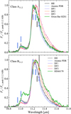 |
Fig. 6 Comparison of the 11.2 µm profile in the five template spectra with a class A 11.2 µm profile represented by the ISO-SWS spectrum of the Orion Bar H2S1 (van Diedenhoven et al. 2004, top panel) and a class B 11.2 µm profile represented by the ISO-SWS spectrum of HD 44179 (van Diedenhoven et al. 2004, bottom panel). |
4.2 AIB profiles
Broadly speaking, the prominent AIBs can be separated into three groups: 1) bands with a steep blue rise and a pronounced red wing. The 5.25, 6.2, and 11.2 µm AIBs are clear examples. The profiles also often show a shoulder on the blue side, which is considerably weaker than the red wing; 2) bands that are clear blends of multiple components. This group includes the 3.4, 5.75, 7.7, and 12.7 µm AIBs. They typically comprise three or more sub-components.; and 3) bands that seem to be symmetric, often resembling Gaussian profiles. This group includes the 3.3, 5.878, and 8.6 µm AIBs, as well as the 6.024 and 11.005 µm AIBs. These divisions are not entirely strict. The group 1 AIBs typically have very weak features perched on the red and/or blue side of the profile. Likewise, it is conceivable that each of the blended components in the group 2 AIBs might have an intrinsic profile with relatively sharp blue rise and a more gradual red wing that is obfuscated by blending. For example, while the 3.403 µm AIB is often blended with a feature at 3.424 µm, this component is very weak and the 3.403 µm profile resembles that of group 1. We note that while the 11.2 µm AIB is also a blend of three components, the character of the profile is dominated by the presence of a steep blue rise and a pronounced red wing rather than the presence of the sub-components. Therefore, we list the 11.2 µm AIB in group 1.
Profiles with a steep blue rise and a pronounced red wing are characteristic for the effects of anharmonicity (Pech et al. 2002; Mackie et al. 2022). Detailed models have been developed that follow the emission cascade for a highly excited, single PAH and that include the effects of anharmonic interactions based on quantum chemical calculations (Mackie et al. 2022). These models do not contain free parameters besides the size of the emitting species (i.e. the average excitation level after absorption of a FUV photon) and the resulting profiles agree qualitatively well with the observations of group 1 AIBs (Mackie et al. 2022). The results show that the wavelength extent of the red wing depends on the details of the anharmonic coupling coefficients with other modes. The strength of the wing relative to the peak emission is sensitive to the excitation level of the emitting species after absorption of the UV photon (i.e. the initial average energy per mode) and the cascade process (e.g. how fast the energy is “leaking” away through radiative cooling). The steepness of the blue rise is controlled by rotational broadening. Analysis of the profile of the 11.2 µm AIB observed by ISO/SWS suggests emission by a modestly sized PAH (NC ~ 30; Mackie et al. 2022) but that conclusion has to be reassessed given the presence of more than one component in this AIB in the JWST spectra of the Orion Bar.
Not all bands will show equally prominent anharmonic profiles. In particular, the far-infrared modes in small PAHs are very harmonic in nature (Lemmens et al. 2020) and their profiles would not develop red wings. Likewise, the aromatic CH stretching modes are very susceptible to resonances with combination bands (Maltseva et al. 2015, 2016; Mackie et al. 2015, 2016) and this interaction dominates their profiles (Mackie et al. 2022).
4.3 AIB variability in Orion
Spatial-spectral maps carry much promise to untangle the complexity of the AIBs and possibly link observed variations to the presence of specific carriers. The first forays into this field were based on Spitɀer spectral maps. Analysis of the spatial behaviour of individual AIBs and AIB components revealed their interdependence as well as new components (e.g. Boersma et al. 2009b, 2013, 2014; Peeters et al. 2012, 2017; Shannon et al. 2016). Analyses based on blind signal separation methods have uncovered several distinct components and spectral details (Berné et al. 2007; Joblin et al. 2008; Pilleri et al. 2012; Foschino et al. 2019), but the increased spectral and spatial resolution, as well as the higher sensitivity of JWST, can be expected to take this to a new level. Indeed, some of the spectral details uncovered by previous spatial-spectral studies are now directly detected in the presented JWST data of the Orion Bar. Applications of blind signal separation techniques, as well as spectral fitting using PAHFIT (Smith et al. 2007) and the Python PAH Database (Shannon & Boersma 2018) on the full spectral map of the Orion Bar may be a promising ground for additional detections and potential identifications. Here, we address spatial-spectral variations on inspection of the five template spectra. More detailed analyses are deferred to future studies.
While the spectra are rich in components (Table A.1), there is little diversity between the template spectra. All templates show evidence for each sub-components, except possibly for a few very weak bands whose presence may be easily lost in the profiles of nearby strong bands. The most obvious variations are the increased prominence of the sub-components in the 7.7 µm AIB at 7.743 and 7.85 µm and in the 11.2 µm AIB at 11.25 µm in the DF 2 and DF 3 spectra, and the variation in the relative strength of the sub-components of the weak 5.75 µm band. Similarly, the width of many AIBs (3.3, 5.25, 6.2, 7.7, 11.2, and 12.7) broadens significantly (Table 1). This broadening is also systematic, with the FWHM being smallest in the atomic PDR, increasing subsequently in DF 1, followed by the H II region, then DF 2, and finally DF 3 (Table 1 and Fig. 5). The only exception to this systematic trend is the H II region having a FWHM smaller than DF 1 (but larger than the atomic PDR) for the 5.25 and 7.7 µm AIBs. As pointed out in Sect. 2.2, we note that the AIB emission in the H II region originates from the background PDR.
There is also some region-to-region variation in the relative strengths of the main AIBs (Fig. 5). The largest variations are seen in the 3.4 µm AIB to 3.3 µm AIB ratio (~100% greater in DF 3 than in the atomic PDR) and in the 3.3 µm AIB to 11.2 µm AIB ratio (~40% greater in DF 3 than in the atomic PDR). Both of these ratios are largest in DF 2 and DF 3, and decrease in the atomic region. Variations in the strength of the CC modes and in-plane CH bending modes (6.2, 7.7, and 8.6 µm) relative to the 11.2 µm OOP modes are more modest (at the 10–20% level). Larger variations occur in the relative strength of the moderate bands, namely, the 5.25, 5.878, 6.024, and 11.955 µm bands – which are much more pronounced in DF 2 and DF 3 than in the atomic zone. As noted in Sect. 4.1, the ISO-SWS data of the Orion Bar resembles the atomic PDR template. Hence, the range in spectral variability within class A AIBs is well represented by the five templates for all AIBs except the 11.2 µm AIB. For the 11.2 µm AIB, the presented data not only showcase the class A AIB variability but also the shifts from class A to class A(B) and then to class B. It is expected that future JWST observations probing a large range of physical conditions and environments further extend the spectral variability in the AIB emission.
The anharmonic profile of bands due to smaller PAHs will tend to have a less steep blue rise due to the increase in the rotational broadening as well as a slight increase in the width and a more pronounced red wing due the higher internal excitation for the same photon energy (Mackie et al. 2022; Tielens 2021). Hence, the presence of somewhat smaller PAHs may be at the origin (of some) of the overall profile variations in the 3.4, 5.25, 6.2, and 11.2 µm AIBs in the JWST template spectra. We note that the spectrum of the DF 1 template resembles much more the atomic region template than the DF 2 and DF 3 dissociation front templates (Figs. 3 and 4, as well as Table 1). This is likely due to the terraced-field-like structure of the molecular PDR resulting in a strongly enhanced line-of-sight visual extinction through the foreground atomic PDR toward DF 1 compared to DF 2 and DF 3 (Habart et al. 2023; Peeters et al. 2024). Hence, a large contribution from the atomic region in the foreground is contributing to the emission toward DF 1. The overall similarity of the spectra suggests that the PAH family is very robust but has a small amount of additional species in the DF 2 and DF 3 zones that is not present in the surface layers of the PDR. In the Orion Bar, the PDR material is advected from the molecular zone to the ionization front at about 1 km s−1 (Pabst et al. 2019) over ≃20 000 yr. In that period, a PAH will have absorbed some 108 UV photons and, yet, apparently the effect on the composition of the interstellar PAH family is only minor as it only results in a change in the prominence of the sub-components in the 7.7 and 11.2 µm AIBs. This likely reflects that for moderate-to-large PAHs (NC ≳ 30), photofragmentation is a minor channel compared to IR emission and, moreover, when fragmentation occurs, the H-loss channel dominates over C loss (Allain et al. 1996a,b; Zhen et al. 2014b,a; Wenzel et al. 2020) and then rapidly followed by rehydrogena-tion with abundant atomic H (Montillaud et al. 2013; Andrews et al. 2016). We note that the UV field increases by about two orders of magnitude between the H2 dissociation front and the PDR surface but the atomic H abundance increases by a similar factor as H2 is increasingly photolysed near the surface. Hence, the ratio of the local FUV field to the atomic hydrogen density, G0/n(H), which controls the photoprocessing (Andrews et al. 2016), does not vary much among the five template regions. We thus suggest that the additional species in the deeper layers of the Orion Bar causing the increased prominence of sub-components in the 5.75 (at 5.755 µm), 7.7, and 11.2 µm AIBs, are aromatic species and/or functional groups and/or pendant rings that are more susceptible to photolysis.
Photolytic processing of the PAH family with position in the Orion Bar may also leave its imprint on the PAH size distribution and this will affect the relative strength of the AIBs. The 3.3/11.2 AIB ratio has long been used as an indicator of the size of the emitting species (Allamandola et al. 1989b; Pech et al. 2002; Ricca et al. 2012; Mori et al. 2012; Croiset et al. 2016; Maragkoudakis et al. 2020; Knight et al. 2021, 2022a) as this ratio is controlled by the 'excitation temperature' of the emitting species and, hence, for a fixed FUV photon energy, by the size. For the five JWST template regions, the 3.3/11.2 AIB ratio is observed to vary by about 40%, being largest in DF 3 and decreasing toward DF 2, followed by DF 1, the atomic PDR and the H II region. The variation in this ratio is slightly less than what is observed in the reflection nebulae NGC 7023 and in the larger Orion region (e.g. the Orion Bar and the Veil region beyond the Orion Bar) and corresponds to an increase in the typical size of the emitting species by about 40% toward the surface (Croiset et al. 2016; Knight et al. 2021, 2022a; Murga et al. 2022). Hence, we link the decreased prominence of the sub-component in the 5.75 µm (at 5.755 µm), 7.7 µm (at 7.743 and 7.775 µm), and 11.2 µm AIBs (at 11.275 µm) as well as the variation in the 3.3/11.2 AIB ratio to the effects of photolysis as material is advected from the deeper layers of the PDR to the surface.
Variations in the 6.2/11.2 ratio (Fig. 5) are generally attributed to variations in the ionised fraction of PAH (Peeters et al. 2002a; Galliano et al. 2008; Stock et al. 2016; Boersma et al. 2018). This ratio is only 12% stronger in DF 3 than the surface of the PDR. The limited variations in the 6.2/11.2 AIB ratio is at odds with those measured by Spitzer and ISO. Specifically, this ratio is observed to increase by about 50% across the Orion Bar when approaching the Trapezium cluster (Knight et al. 2022a). Moreover, Galliano et al. (2008) measured an increase in this ratio by almost a factor of 2 over (a much wider swath of) the Orion Bar. The PAH ionization balance is controlled by the ionization parameter, G0T1/2/ne with G0, T, and ne the intensity of the FUV field, the gas temperature, and the electron density. The high spatial resolution of JWST allows for a clear separation of the emission at the H2 dissociation fronts and the PDR surface. The limited variation in the 6.2/11.2 AIB ratio is somewhat surprising because the PAH ionizing photon flux differs by about a factor of 40 between the dissociation fronts (located at AV = 2 mag) and the PDR surface; the gas temperature will also increase (slightly) toward the surface, while the electron abundance remains constant over this region (Tielens & Hollenbach 1985). It is also possible that PAH cations contribute an appreciable amount to the 11.2 µm band (Shannon et al. 2016; Boersma et al. 2018). Further modelling will be important to fully understand the complexity of the Orion Bar (Sidhu et al., in prep.).
The 3.4/3.3 AIB ratio is observed to decrease by about 100% from DF 3 to the atomic PDR (Fig. 5). Such variations have also been seen in other nebulae and attributed to photofragmentation processes (Joblin et al. 1996). The 3.4 µm AIB is attributed to aliphatic CH modes in the form of a minor amount of H bonded to sp3 C atoms either in the form of methyl groups or as super-hydrogenated PAHs (Schutte et al. 1993; Bernstein et al. 1996; Joblin et al. 1996). The abundance of superhydrogenated PAHs is expected to be very small throughout the Orion Bar as such extra H’s are readily lost in the strong FUV radiation field (Andrews et al. 2016). Methyl groups are also more easily photolysed than aromatic H’s (energy barriers are 3.69, 4.00, and 4.47 eV for CH2-H, -CH3 and aromatic H loss, respectively; Tielens 2021). Recent experiments report that, for cations, this methyl group photolysis can lead to quite stable tropylium formation (loss of H followed by isomerization to a seven-membered ring; Jochims et al. 1999; Zhen et al. 2016; Wenzel et al. 2022). However, further investigation is required to firmly establish the importance of this fragmentation route for conditions present in the interstellar medium. If borne out, the reaction of the tropylium cation with atomic H has a calculated barrier of 3.2 kcal mol–1 (1600 K; Bullins et al. 2009) and, hence, under warm, dense H-rich conditions, the methyl group could be reformed. Hence, in a "suitable" PDR, the species may cycle back and forth between a methyl functional group and the tropylium structure until eventually −CH3 loss occurs. In any case, it can be expected that the stronger UV field nearer to the surface will reduce the number of CH methyl groups compared to the number of CH aromatic bonds. Further experimental and quantum chemical studies will have to address the competition between the various channels involved in the chemistry of methylated PAHs in PDRs.
The increased importance of PAH photolysis near the surface of the Orion Bar PDR is in line with the GrandPAH hypothesis that only the most resilient species can sustain the harsh conditions of strong FUV radiation fields. Thus, a limited number of compact, large PAHs will dominate the interstellar PAH family in these conditions (Andrews et al. 2015; Tielens 2013). If the conditions are right, large PAHs may even be stripped of all their H’s and isomerize to the fullerene, C60 (Boersma et al. 2012; Berné et al. 2015; Zhen et al. 2014a). We also realize that the presence of somewhat smaller PAHs and the increased importance of aliphatic functional groups deep in the PDR may reflect the importance of ion-molecule and/or radical chemistry during the preceding dark cloud core phase modifying and/or forming PAHs in a bottom-up scenario akin to that proposed for the formation of benzonitrile, indene, and cyanonaphthalene (McGuire et al. 2018, 2021; Cernicharo et al. 2021).
5 Conclusions
The superb sensitivity and spectral resolution of JWST have revealed an ever-better characterization of the AIBs in the Orion Bar in terms of sub-components, multiple components making up a "single" band, and band profiles. In addition, the unprecedented spatial resolution of the spectral imaging data showcases the interdependence of the numerous AIB components.
We extracted five template spectra in apertures positioned on the H II region, the atomic PDR, and the three dissociation fronts DFs 1, 2, and 3. The spectra display a wealth of detail and many weak features have now been firmly identified, their peak positions quantified, and their profiles established. At the same time, the spectra are really very simple. There are a limited number of strong bands with well defined peak positions and red-shaded profiles characteristic for anharmonic interactions. And there is little diversity between the templates. A modest variation is observed in the relative intensities of the main AIBs and of the sub-components of an AIB as well as a systematic broadening of the FWHM of many AIBs (smallest in the atomic PDR and largest in DF 3). Consequently, these templates demonstrate the spectral variations in the class A AIB emission as well as the shift from class B112 (DF 3) to class A11.2 (atomic PDR). The comparison of the template spectra with the ISO-SWS spectrum of the Orion Bar underscores that the spectrum of the atomic region is the "poster child" for the class A spectrum (Fig. 2; Peeters et al. 2002a; van Diedenhoven et al. 2004). This comparison also demonstrates that in a large aperture, PDRs such as Orion are expected to show class A spectra. Conversely, PDRs with more gentle physical conditions (e.g. in the DF 3) are expected to display a slightly modified class A AIB spectrum (except for the 11.2 µm AIB), showcasing broader AIBs and an increased prominence of minor sub-components with respect to the exemplar class A spectrum. In the case of the 11.2 µ m AIB, more gentle physical conditions broaden the AIB and increase the prominence of minor sub-components seen in class A, resulting in a class B 11.2 µm AIB profile. Hence, the templates suggest a shift from class B11.2 (DF 3) to class A11.2 (atomic PDR). Further modelling of the PDR physics and chemistry may help to pinpoint the physical and chemical processes that drive these spatial-spectral variations in the Orion Bar. Furthermore, we expect that similar studies of a variety of sources with JWST will provide deeper insight in the origin of the A, B, C, and D classes identified by using measurements obtained with ISO and Spitzer (Peeters et al. 2002a; van Diedenhoven et al. 2004; Sloan et al. 2014; Matsuura et al. 2014). In any case, the spatial-spectral variations in the Orion Bar provide a framework in which AIB spectra of extragalactic regions of massive star formation can be analysed in terms of the physical conditions in their PDRs.
An analysis of the Spitzer spectra of a variety of objects revealed that the mid-IR spectra at the brightest spots in PDRs show remarkably similar AIBs and this has been taken to imply that in the harsh conditions of these positions, the PAH family is dominated by a few species that can withstand the harsh conditions in PDRs (Andrews et al. 2015; Tielens 2013). For now, the limited diversity in the AIB characteristics of the Orion Bar templates points in the same direction. Indeed, a broad distribution of PAHs would result in much more sub-structure and variation behavior. In addition, the disappearance of the (weak) 11.25 µm component of the 11.2 µm AIB in the PDR surface layers implies that photochemistry is important: only the most robust species survive in the harsh conditions at the surface of the PDR. We note that while the cosmic AIB emission can be classified in four classes (A, B, C, and D), interstellar AIB emission invariably belongs to class A. The Orion Bar spectrum is the "poster child" of the class A spectrum - out of all the AIBs found in the Orion Bar template spectra, only the 11.2 µm AIB shows some indication of a class B contribution. Only very distinctly different classes of objects with unique histories display classes B, C, and D AIB emission. This too implies that the interstellar PAH family consists of a small set of very robust species.
Moreover, we conclude that the profiles of the 5.25, 6.2, and 11.2 µ m AIBs are controlled by anharmonicity, rather than by blending of a number of bands, while variations in the widths of these bands in the different template spectra are related to variations in the excitation of the emitting species in those positions. As a corollary, this implies that these bands are likely dominated by emission of a single carrier, further supporting the GrandPAH hypothesis (Mackie et al. 2022). However, it remains to be seen whether this spectral similarity still holds when a much larger range of objects is investigated at the higher spectral resolution of JWST.
The much higher spatial resolution of JWST provides further insight in the processes that might be relevant for the composition of the PAH family. Specifically, as argued in Sect. 4, the decreased prominence of the minor features in the 5.75, 7.7, and 11.2 µm AIBs in the atomic region indicates the loss of a sub-population of the PAH family (Berné & Tielens 2012; Montillaud et al. 2013; Berné et al. 2015; Andrews et al. 2016) or the loss of very small grains (Pilleri et al. 2012, 2015) in this region. Likewise, the decrease in the methyl group coverage, as evidenced in the variation of the 3.4/3.3 AIB ratio, indicates the loss of more loosely bound functional groups in the surface layers or their conversion to aromatic moieties. Models suggest that photolysis of PAHs is controlled by the strength of the UV field over the atomic hydrogen density (Montillaud et al. 2013; Andrews et al. 2016; Berné et al. 2015) and over much of the Orion Bar PDR, G0/n(H) ≃ 1 (Tielens & Hollenbach 1985; Bernard-Salas et al. 2012), implying that the PAHs that are lost from the PAH family are small (NC ≲ 50).
Hence, the picture that emerges from the analysis of the template spectra is the increased importance of FUV processing in PDR surface layers, resulting in a "weeding out" of the weakest links of the PAH family. These less resistant species are possibly formed from small hydrocarbons during the preceding dark cloud phase of the region in a bottom-up chemical scenario (Cuadrado et al. 2015; McGuire et al. 2021), feeding the gas with small hydrogen rich photolytically produced species (Alata et al. 2015). The UV processing of the PAH family will start with the loss of the smallest PAHs but as the PDR material is advected to the surface, larger and larger PAHs will become susceptible to photoprocessing. Similar scenarios have been proposed recently with data not obtained with JWST, albeit with slightly different numbers (e.g. NC ≲ 50 in Murga et al. 2022). In favourable conditions, the processing of very large PAHs (NC ≳ 60) may lead to the formation of C60 (Berné & Tielens 2012; Berné et al. 2015). While the present data around 18.9 µm are still marred by instrumental artefacts, future searches for the signature of fullerenes in the MIRI spectra of these surface layers may reveal whether such a scenario plays a role under the conditions of the Orion Bar.
JWST is poised to obtain high-quality spectral imaging observations of a large sample of environments probing the full range of physical conditions that are relevant for AIB emission. These observations promise to capture the complexity of AIB emission with the unprecedented detail that is needed in order to advance our understanding of the photochemical evolution of large carbonaceous molecules.
Acknowledgements
We thank the referee, Alan Tokunaga, for constructive comments on the manuscript. We are very grateful to the JWST Help Desk for their support with pipeline and calibration issues that were encountered while writing this paper. This work is based on observations made with the NASA/ESA/CSA James Webb Space Telescope. The data were obtained from the Mikulski Archive for Space Telescopes at the Space Telescope Science Institute, which is operated by the Association of Universities for Research in Astronomy, Inc., under NASA contract NAS 5-03127 for JWST. These observations are associated with program #1288. Support for program #1288 was provided by NASA through a grant from the Space Telescope Science Institute, which is operated by the Association of Universities for Research in Astronomy, Inc., under NASA contract NAS 5-03127. E.P. and J.C. acknowledge support from the University of Western Ontario, the Institute for Earth and Space Exploration, the Canadian Space Agency (CSA; 22JWGO1- 16), and the Natural Sciences and Engineering Research Council of Canada. Studies of interstellar PAHs at Leiden Observatory (AT) are supported by a Spinoza premie from the Dutch Science Agency, NWO. C.B. is grateful for an appointment at NASA Ames Research Center through the San José State University Research Foundation (80NSSC22M0107). Part of this work was supported by the Programme National "Physique et Chimie du Milieu Interstellaire" (PCMI) of CNRS/INSU with INC/INP co-funded by CEA and CNES. J.R.G. and S.C. thank the Spanish MCINN for funding support under grant PID2019-106110GB-I00. T.O. is supported by JSPS Bilateral Program, Grant Number 120219939. Work by Y.O. and M.R. is carried out within the Collaborative Research Centre 956, sub-project C1, funded by the Deutsche Forschungsgemeinschaft (DFG) – project ID 184018867. This work was also partly supported by the Spanish program Unidad de Excelencia María de Maeztu CEX2020-001058-M, financed by MCIN/AEI/10.13039/501100011033. N.N. is funded by the United Arab Emirates University (UAEU) through UAEU Program for Advanced Research (UPAR) grant G00003479. A.P. (Amit Pathak) would like to acknowledge financial support from Department of Science and Technology - SERB via Core Research Grant (DST-CRG) grant (SERB-CRG/2021/000907), Institutes of Eminence (IoE) incentive grant, BHU (incentive/2021-22/32439), Banaras Hindu University, Varanasi and thanks the Inter-University Centre for Astronomy and Astrophysics, Pune for associateship. This work is sponsored (in part) by the CAS, through a grant to the CAS South America Center for Astronomy (CASSACA) in Santiago, Chile. A.R. gratefully acknowledges support from the directed Work Package at NASA Ames titled: 'Laboratory Astrophysics -The NASA Ames PAH IR Spectroscopic Database'. M.B. acknowledges DST for the DST INSPIRE Faculty fellowship. H.Z. acknowledges support from the Swedish Research Council (contract no. 2020-03437). P.M. acknowledges grants EUR2021-122006, TED2021-129416A-I00 and PID2021-125309OA-I00 funded by MCIN/AEI/ 10.13039/501100011033 and European Union NextGener-ationEU/PRTR. M.S.K. is funded by RSCF, grant number 21-12-00373.
Appendix A Inventory of AlBs
Table A.1 shows the inventory of AIBs identified in this study.
Catalogue of AIB features detected in the five template spectra of the Orion Bar. The method used to select these features is described in Sect. 3. The precise peak positions of nominal AIBs – whose wavelengths appear in boldface in this table – are indicated in Col. 3. We note that we converted the positions in wavelength to wavenumber by rounding to the nearest integer in units of cm−1, and so the precision of the reported wavenumbers do not reflect the precision of the peak position of the AIBs.
Appendix B The impact of residual artefacts in the data
At the time of writing, there are two types of artifacts in the data that sometimes have appearances similar to AIBs. Firstly, the constructive and destructive interference of layers in the MIRI detector arrays leads to periodic variations in the observed signal versus wavelength called “fringes” (Argyriou et al. 2020). The latest versions of the JWST pipeline and calibration reference files greatly reduce, but do not completely remove all fringes. These residual fringes can sometimes be difficult to distinguish from AIB components.
Secondly, at the moment, the absolute flux calibration of JWST (Gordon et al. 2022) is based on a single A star (private communication with the JWST Help Desk). Intrinsic spectral differences between the star that was used for calibration and the true spectrum of a given source can lead to artifacts in the observed spectrum of that source. Some artifacts are more complicated couplings between instrumental effects and incomplete absolute flux calibration.
Non-exhaustive list of wavelengths of artifacts:
- 1.
Excess emission: 14.3, 14.35 µm
- 2.
Excess absorption: ~12.2, 13.71–13.77, 13.77–13.8, 13.85– 13.95 µm
- 3.
Fringes: 10–12 µm with an amplitude of about 5% (affects red tail of 11.2)
While future versions of the pipeline and reference files will fix fringes and calibration issues, we have developed a temporary fix for our analysis. We use MIRI-MRS observations of 10 Lac, which is an O9V star from the JWST CALSPEC7 program (Bohlin et al. 2014). These data were reduced with the same versions of the JWST pipeline and CRDS files that were used when reducing the Orion Bar data. Then we extracted the MIRI spectrum of 10 Lac using apertures whose radii increase linearly with wavelength. A comparison of the extracted spectrum and the CALSPEC model spectrum of 10 Lac revealed offsets in addition to fringes and absorption/emission artifacts. To deal with these offsets which vary from subband to subband, we performed linear regression on the extracted flux versus the model flux within a given subband, and then corrected the observed spectrum using the best-fit parameters for that subband. We then compute the ratio of the corrected, observed 10 Lac flux, to the model flux
 (B.1)
(B.1)
where  . is the (corrected) observed 10 Lac spectrum, and
  is the model spectrum. Artifacts in the observed 10 Lac spectrum show up as deviations in CV away from 1.0. We use CV to correct the Orion template spectra
  ,
,
![Mathematical equation: $F_v^{{\rm{corr}}{\rm{.}}}\left[ {{\rm{MJy}}\,\,{\rm{s}}{{\rm{r}}^{ - 1}}} \right] = F_v^{{\rm{obs}}{\rm{.}}}/\left( {{A_{{\rm{chan}}{\rm{., band}}}}\left( {{C_v} - 1} \right) + 1} \right){\rm{,}}$](/articles/aa/full_html/2024/05/aa46662-23/aa46662-23-eq5.png) (B.2)
(B.2)
where Achan,band is a parameter to adjust the amplitude of the correction for a given channel and subband. We apply corrections to Channel 2 LONG, Channel 3 MEDIUM, and Channel 3 LONG, using Achan,band = 0.5,0.25,1.0, respectively (these factors were chosen manually). For all other wavelength ranges, no correction was applied either because no fringes were visible, or the correction introduced noise, making it difficult to tell if the fringes were actually corrected or simply buried in noise.
Examples of uncorrected template spectra are shown in Fig. B.1. Fringes and absorption/emission artifacts in 10 Lac (the green curve) are detected at the same wavelengths in the Orion data. In Fig. B.2 we show the H II region template spectrum before and after applying the correction described above. The correction efficiently removes fringes (the first three panels), excess absorption (fourth panel), and excess emission artifacts (bottom panel) which would have otherwise been incorrectly classified as AIB emission. We also conclude that the terraces in the 12.7 µm AIB are real. We note however that some residual calibration issues remain, in particular at the longer wavelengths. We therefore restricted our analysis to wavelengths shorter than 15 µm with the exception of the addition of the moderately strong 16.4 µm AIB. We note that an artefact is also present at 18.9 µm. This wavelength corresponds to the strongest band of C60 emission (Cami et al. 2010; Sellgren et al. 2010). Unfortunately, due to the artefact, we are currently unable to confirm (or refute) the detection of C60 in these templates. In addition, the 12.2 µm absorption feature is due to a spectral leak (estimated to be ~3% of the 6.1 µm signal; JWST Help Desk). This leak also affected the calibration star resulting in an incorrect photometric correction in the current pipeline. Due to the different spectral shape of Orion with respect to the calibration star, this resulted in the observed absorption feature and our applied correction is unable to correct this. This artefact influences the 12.0 and 12.7 µm AIBs.
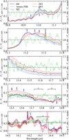 |
Fig. B.1 Zoom-ins on continuum-subtracted template spectra (not corrected for calibration issues, i.e. |

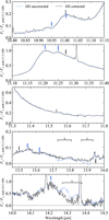 |
Fig. B.2
|

Appendix C Continuum determination
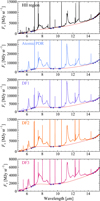 |
Fig. C.1 The MIRI-MRS template spectra with their respective con-tinua. The anchor points for each continuum are represented by filled circles. See Sect. 2.3 and Appendix C for details. |
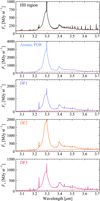 |
Fig. C.2 The NIRSpec template spectra (grating g395h, filter f290lp) from Peeters et al. (2024) along with their respective continua, zoomed in on the wavelength range that is relevant to the 3.3 µm AIB. See Sect. 2.3 and Appendix C for details. |
Here we show the continuum curves and the anchor points that were used to estimate them. Figure C.1 shows the MIRI MRS template spectra and continua, while Figure C.2 shows the same but for NIRSpec data.
For the 3 µm region (NIRSpec templates), we fit a linear continuum to the wavelength ranges [3.05, 3.07], [3.667, 3.689], and [3.7068, 3.720], chosen to avoid emission lines. For the MIR (MIRI templates), we compute a cubic spline interpolation (tension of 1.0, IDL) anchored at selected wavelengths to estimate the continuum emission. We selected anchor points that avoid all (weak) AIBs in all five templates. This resulted in anchor points at 5.011, 5.042, 5.073, 5.487, 5.948, 6.576, 6.785, 7.013, 9.131, 9.440,10.191,10.344,14.642,14.913,15.178,15.461,19.349, and 19.632 µm. The resulting continuum is shown in Fig. C.1. Our choice to use the same anchor points for all templates leads to slightly-overestimated continuum at 5.5 µm in the DF 3 and at 7.1 µm in the H II region. Subtracting slightly-overestimated continuum from the templates will affect the resulting AIB emission in some cases.
References
- Alata, I., Jallat, A., Gavilan, L., et al. 2015, A&A, 584, A123 [NASA ADS] [CrossRef] [EDP Sciences] [Google Scholar]
- Allain, T., Leach, S., & Sedlmayr, E. 1996a, A&A, 305, 602 [NASA ADS] [Google Scholar]
- Allain, T., Leach, S., & Sedlmayr, E. 1996b, A&A, 305, 616 [NASA ADS] [Google Scholar]
- Allamandola, L. J., Tielens, A. G. G. M., & Barker, J. R. 1985, ApJ, 290, L25 [Google Scholar]
- Allamandola, L. J., Bregman, J. D., Sandford, S. A., et al. 1989a, ApJ, 345, L59 [NASA ADS] [CrossRef] [Google Scholar]
- Allamandola, L. J., Tielens, A. G. G. M., & Barker, J. R. 1989b, ApJS, 71, 733 [Google Scholar]
- Allamandola, L. J., Hudgins, D. M., & Sandford, S. A. 1999, ApJ, 511, L115 [Google Scholar]
- Andrews, H., Boersma, C., Werner, M. W., et al. 2015, ApJ, 807, 99 [NASA ADS] [CrossRef] [Google Scholar]
- Andrews, H., Candian, A., & Tielens, A. G. G. M. 2016, A&A, 595, A23 [NASA ADS] [CrossRef] [EDP Sciences] [Google Scholar]
- Argyriou, I., Wells, M., Glasse, A., et al. 2020, A&A, 641, A150 [NASA ADS] [CrossRef] [EDP Sciences] [Google Scholar]
- Argyriou, I., Glasse, A., Law, D. R., et al. 2023, A&A, 675, A111 [NASA ADS] [CrossRef] [EDP Sciences] [Google Scholar]
- Arnoult, K. M., Wdowiak, T. J., & Beegle, L. W. 2000, ApJ, 535, 815 [NASA ADS] [CrossRef] [Google Scholar]
- Bakes, E. L. O., Tielens, A. G. G. M., & Bauschlicher, C. W. 2001, ApJ, 556, 501 [NASA ADS] [CrossRef] [Google Scholar]
- Bauschlicher, C. W. J., & Ricca, A. 2014, Theor. Chem. Acc., 133, 1454 [CrossRef] [Google Scholar]
- Bauschlicher, Charles W. J., Peeters, E., & Allamandola, L. J. 2008, ApJ, 678, 316 [NASA ADS] [CrossRef] [Google Scholar]
- Bauschlicher, C. W., Peeters, E., & Allamandola, L. J. 2009, ApJ, 697, 311 [NASA ADS] [CrossRef] [Google Scholar]
- Beintema, D. A., van den Ancker, M. E., Molster, F. J., et al. 1996, A&A, 315, L369 [Google Scholar]
- Bernard-Salas, J., Habart, E., Arab, H., et al. 2012, A&A, 538, A37 [NASA ADS] [CrossRef] [EDP Sciences] [Google Scholar]
- Berné, O., & Tielens, A. G. G. M. 2012, PNAS, 109, 401 [CrossRef] [Google Scholar]
- Berné, O., Joblin, C., Deville, Y., et al. 2007, A&A, 469, 575 [NASA ADS] [CrossRef] [EDP Sciences] [Google Scholar]
- Berné, O., Montillaud, J., & Joblin, C. 2015, A&A, 577, A133 [NASA ADS] [CrossRef] [EDP Sciences] [Google Scholar]
- Berné, O., Habart, É., Peeters, E., et al. 2022, PASP, 134, 054301 (Paper I) [CrossRef] [Google Scholar]
- Bernstein, M. P., Sandford, S. A., & Allamandola, L. J. 1996, ApJ, 472, L127 [NASA ADS] [CrossRef] [Google Scholar]
- Boersma, C., Mattioda, A. L., Bauschlicher, C. W., et al. 2009a, ApJ, 694, 704 [NASA ADS] [CrossRef] [Google Scholar]
- Boersma, C., Mattioda, A. L., Bauschlicher, C. W., J., et al. 2009b, ApJ, 690, 1208 [NASA ADS] [CrossRef] [Google Scholar]
- Boersma, C., Rubin, R. H., & Allamandola, L. J. 2012, ApJ, 753, 168 [NASA ADS] [CrossRef] [Google Scholar]
- Boersma, C., Bregman, J. D., & Allamandola, L. J. 2013, ApJ, 769, 117 [NASA ADS] [CrossRef] [Google Scholar]
- Boersma, C., Bregman, J., & Allamandola, L. J. 2014, ApJ, 795, 110 [NASA ADS] [CrossRef] [Google Scholar]
- Boersma, C., Bregman, J., & Allamandola, L. J. 2018, ApJ, 858, 67 [NASA ADS] [CrossRef] [Google Scholar]
- Bohlin, R. C., Gordon, K. D., & Tremblay, P. E. 2014, PASP, 126, 711 [NASA ADS] [Google Scholar]
- Böker, T., Arribas, S., Lützgendorf, N., et al. 2022, A&A, 661, A82 [NASA ADS] [CrossRef] [EDP Sciences] [Google Scholar]
- Boulanger, F., Reach, W. T., Abergel, A., et al. 1996, A&A, 315, L325 [NASA ADS] [Google Scholar]
- Bouwman, J., Henning, T., Hillenbrand, L. A., et al. 2008, ApJ, 683, 479 [NASA ADS] [CrossRef] [Google Scholar]
- Bregman, J. 1989, in IAU Symp. 135: Interstellar Dust, 135, 109 [Google Scholar]
- Bregman, J., & Temi, P. 2005, ApJ, 621, 831 [CrossRef] [Google Scholar]
- Bregman, J. D., Allamandola, L. J., Witteborn, F. C., Tielens, A. G. G. M., & Geballe, T. R. 1989, ApJ, 344, 791 [NASA ADS] [CrossRef] [Google Scholar]
- Bullins, K. W., Huang, T. T. S., & Kirkby, S. J. 2009, Int. J. Quant. Chem., 109, 1322 [NASA ADS] [CrossRef] [Google Scholar]
- Buragohain, M., Pathak, A., Sakon, I., & Onaka, T. 2020, ApJ, 892, 11 [NASA ADS] [CrossRef] [Google Scholar]
- Cami, J., Bernard-Salas, J., Peeters, E., & Malek, S. E. 2010, Science, 329, 1180 [NASA ADS] [CrossRef] [Google Scholar]
- Candian, A., & Sarre, P. J. 2015, MNRAS, 448, 2960 [NASA ADS] [CrossRef] [Google Scholar]
- Candian, A., Kerr, T. H., Song, I. O., McCombie, J., & Sarre, P. J. 2012, MNRAS, 426, 389 [NASA ADS] [CrossRef] [Google Scholar]
- Carpentier, Y., Féraud, G., Dartois, E., et al. 2012, A&A, 548, A40 [NASA ADS] [CrossRef] [EDP Sciences] [Google Scholar]
- Cernicharo, J., Agúndez, M., Cabezas, C., et al. 2021, A&A, 649, L15 [EDP Sciences] [Google Scholar]
- Cohen, M., Tielens, A. G. G. M., Bregman, J., et al. 1989, ApJ, 341, 246 [NASA ADS] [CrossRef] [Google Scholar]
- Croiset, B. A., Candian, A., Berné, O., & Tielens, A. G. G. M. 2016, A&A, 590, A26 [NASA ADS] [CrossRef] [EDP Sciences] [Google Scholar]
- Cuadrado, S., Goicoechea, J. R., Pilleri, P., et al. 2015, A&A, 575, A82 [NASA ADS] [CrossRef] [EDP Sciences] [Google Scholar]
- Dartois, E., Muñoz Caro, G. M., Deboffle, D., & d’Hendecourt, L. 2004, A&A, 423, L33 [NASA ADS] [CrossRef] [EDP Sciences] [Google Scholar]
- Dartois, E., Muñoz Caro, G. M., Deboffle, D., Montagnac, G., & D’Hendecourt, L. 2005, A&A, 432, 895 [NASA ADS] [CrossRef] [EDP Sciences] [Google Scholar]
- Dartois, E., Charon, E., Engrand, C., Pino, T., & Sandt, C. 2020, A&A, 637, A82 [NASA ADS] [CrossRef] [EDP Sciences] [Google Scholar]
- de Graauw, T., Haser, L. N., Beintema, D. A., et al. 1996, A&A, 315, L49 [NASA ADS] [Google Scholar]
- Dubosq, C., Pla, P., Dartois, E., & Simon, A. 2023, A&A, 670, A175 [NASA ADS] [CrossRef] [EDP Sciences] [Google Scholar]
- Esquej, P., Alonso-Herrero, A., González-Martín, O., et al. 2014, ApJ, 780, 86 [Google Scholar]
- Foschino, S., Berné, O., & Joblin, C. 2019, A&A, 632, A84 [EDP Sciences] [Google Scholar]
- Galliano, F., Madden, S. C., Tielens, A. G. G. M., Peeters, E., & Jones, A. P. 2008, ApJ, 679, 310 [Google Scholar]
- Galué, H. Á. 2014, Chem. Sci., 5, 2667 [CrossRef] [Google Scholar]
- Genzel, R., Lutz, D., Sturm, E., et al. 1998, ApJ, 498, 579 [Google Scholar]
- Gillett, F. C., Forrest, W. J., & Merrill, K. M. 1973, ApJ, 183, 87 [NASA ADS] [CrossRef] [Google Scholar]
- Godard, M., Féraud, G., Chabot, M., et al. 2011, A&A, 529, A146 [NASA ADS] [CrossRef] [EDP Sciences] [Google Scholar]
- Goicoechea, J. R., Pety, J., Cuadrado, S., et al. 2016, Nature, 537, 207 [Google Scholar]
- Gordon, K. D., Bohlin, R., Sloan, G. C., et al. 2022, AJ, 163, 267 [NASA ADS] [CrossRef] [Google Scholar]
- Habart, É., Peeters, E., Berné, O., et al. 2023, A&A, 685, A73 [Google Scholar]
- Hony, S., Van Kerckhoven, C., Peeters, E., et al. 2001, A&A, 370, 1030 [CrossRef] [EDP Sciences] [Google Scholar]
- Houck, J. R., Roellig, T. L., van Cleve, J., et al. 2004, ApJS, 154, 18 [NASA ADS] [CrossRef] [Google Scholar]
- Hudgins, D. M., & Allamandola, L. J. 1999, ApJ, 516, L41 [CrossRef] [Google Scholar]
- Hudgins, D. M., Bauschlicher, Charles W., J., & Allamandola, L. J. 2005, ApJ, 632, 316 [NASA ADS] [CrossRef] [Google Scholar]
- Jensen, J. J., Hönig, S. F., Rakshit, S., et al. 2017, MNRAS, 470, 3071 [NASA ADS] [CrossRef] [Google Scholar]
- Joalland, B., Simon, A., Marsden, C. J., & Joblin, C. 2009, A&A, 494, 969 [NASA ADS] [CrossRef] [EDP Sciences] [Google Scholar]
- Joblin, C., Boissel, P., Leger, A., D’Hendecourt, L., & Defourneau, D. 1995, A&A, 299, 835 [Google Scholar]
- Joblin, C., Tielens, A. G. G. M., Allamandola, L. J., & Geballe, T. R. 1996, ApJ, 458, 610 [NASA ADS] [CrossRef] [Google Scholar]
- Joblin, C., Szczerba, R., Berné, O., & Szyszka, C. 2008, A&A, 490, 189 [NASA ADS] [CrossRef] [EDP Sciences] [Google Scholar]
- Joblin, C., Bron, E., Pinto, C., et al. 2018, A&A, 615, A129 [NASA ADS] [CrossRef] [EDP Sciences] [Google Scholar]
- Jochims, H. W., Baumgärtel, H., & Leach, S. 1999, ApJ, 512, 500 [NASA ADS] [CrossRef] [Google Scholar]
- Jones, A. P., Fanciullo, L., Köhler, M., et al. 2013, A&A, 558, A62 [NASA ADS] [CrossRef] [EDP Sciences] [Google Scholar]
- Kessler, M. F., Steinz, J. A., Anderegg, M. E., et al. 1996, A&A, 315, L27 [NASA ADS] [Google Scholar]
- Knight, C., Peeters, E., Stock, D. J., Vacca, W. D., & Tielens, A. G. G. M. 2021, ApJ, 918, 8 [NASA ADS] [CrossRef] [Google Scholar]
- Knight, C., Peeters, E., Tielens, A. G. G. M., & Vacca, W. D. 2022a, MNRAS, 509, 3523 [Google Scholar]
- Knight, C., Peeters, E., Wolfire, M., & Stock, D. J. 2022b, MNRAS, 510, 4888 [CrossRef] [Google Scholar]
- Léger, A., & Puget, J. L. 1984, A&A, 137, L5 [Google Scholar]
- Lemmens, A. K., Rap, D. B., Thunnissen, J. M. M., et al. 2019, A&A, 628, A130 [EDP Sciences] [Google Scholar]
- Lemmens, A. K., Rap, D. B., Thunnissen, J. M. M., et al. 2020, J. Phys. Chem. Lett., 11, 8997 [CrossRef] [Google Scholar]
- Lemmens, A. K., Rijs, A. M., & Buma, W. J. 2021, ApJ, 923, 238 [NASA ADS] [CrossRef] [Google Scholar]
- Lutz, D., Spoon, H. W. W., Rigopoulou, D., Moorwood, A. F. M., & Genzel, R. 1998, ApJ, 505, L103 [NASA ADS] [CrossRef] [Google Scholar]
- Mackie, C. J., Candian, A., Huang, X., et al. 2015, J. Chem. Phys., 143, 224314 [Google Scholar]
- Mackie, C. J., Candian, A., Huang, X., et al. 2016, J. Chem. Phys., 145, 084313 [NASA ADS] [CrossRef] [Google Scholar]
- Mackie, C. J., Candian, A., Huang, X., et al. 2018, Phys. Chem. Chem. Phys. (Incorp. Faraday Trans.), 20, 1189 [Google Scholar]
- Mackie, C. J., Candian, A., Lee, T. J., & Tielens, A. G. G. M. 2022, J. Phys. Chem. A, 126, 3198 [CrossRef] [Google Scholar]
- Maltseva, E., Petrignani, A., Candian, A., et al. 2015, ApJ, 814, 23 [Google Scholar]
- Maltseva, E., Petrignani, A., Candian, A., et al. 2016, ApJ, 831, 58 [CrossRef] [Google Scholar]
- Maltseva, E., Mackie, C. J., Candian, A., et al. 2018, A&A, 610, A65 [NASA ADS] [CrossRef] [EDP Sciences] [Google Scholar]
- Maragkoudakis, A., Peeters, E., & Ricca, A. 2020, MNRAS, 494, 642 [NASA ADS] [CrossRef] [Google Scholar]
- Marconi, A., Testi, L., Natta, A., & Walmsley, C. M. 1998, A&A, 330, 696 [NASA ADS] [Google Scholar]
- Matsuura, M., Bernard-Salas, J., Lloyd Evans, T., et al. 2014, MNRAS, 439, 1472 [NASA ADS] [CrossRef] [Google Scholar]
- McGuire, B. A., Burkhardt, A. M., Kalenskii, S., et al. 2018, Science, 359, 202 [Google Scholar]
- McGuire, B. A., Loomis, R. A., Burkhardt, A. M., et al. 2021, Science, 371, 1265 [Google Scholar]
- Meeus, G., Waters, L. B. F. M., Bouwman, J., et al. 2001, A&A, 365, 476 [CrossRef] [EDP Sciences] [Google Scholar]
- Menten, K. M., Reid, M. J., Forbrich, J., & Brunthaler, A. 2007, A&A, 474, 515 [NASA ADS] [CrossRef] [EDP Sciences] [Google Scholar]
- Montillaud, J., Joblin, C., & Toublanc, D. 2013, A&A, 552, A15 [NASA ADS] [CrossRef] [EDP Sciences] [Google Scholar]
- Mori, T. I., Sakon, I., Onaka, T., et al. 2012, ApJ, 744, 68 [NASA ADS] [CrossRef] [Google Scholar]
- Murga, M. S., Kirsanova, M. S., Wiebe, D. S., & Boley, P. A. 2022, MNRAS, 509, 800 [Google Scholar]
- Pabst, C., Higgins, R., Goicoechea, J. R., et al. 2019, Nature, 565, 618 [NASA ADS] [CrossRef] [Google Scholar]
- Parmar, P. S., Lacy, J. H., & Achtermann, J. M. 1991, ApJ, 372, L25 [CrossRef] [Google Scholar]
- Pech, C., Joblin, C., & Boissel, P. 2002, A&A, 388, 639 [NASA ADS] [CrossRef] [EDP Sciences] [Google Scholar]
- Peeters, E., Hony, S., Van Kerckhoven, C., et al. 2002a, A&A, 390, 1089 [NASA ADS] [CrossRef] [EDP Sciences] [Google Scholar]
- Peeters, E., Martín-Hernández, N. L., Damour, F., et al. 2002b, A&A, 381, 571 [NASA ADS] [CrossRef] [EDP Sciences] [Google Scholar]
- Peeters, E., Allamandola, L. J., Hudgins, D. M., Hony, S., & Tielens, A. G. G. M. 2004a, ASP Conf. Ser., 309, 141 [NASA ADS] [Google Scholar]
- Peeters, E., Spoon, H. W. W., & Tielens, A. G. G. M. 2004b, ApJ, 613, 986 [NASA ADS] [CrossRef] [Google Scholar]
- Peeters, E., Tielens, A. G. G. M., Allamandola, L. J., & Wolfire, M. G. 2012, ApJ, 747, 44 [NASA ADS] [CrossRef] [Google Scholar]
- Peeters, E., Bauschlicher, Charles W., J., Allamandola, L. J., et al. 2017, ApJ, 836, 198 [NASA ADS] [CrossRef] [Google Scholar]
- Peeters, E., Berné, O., Habart, É., et al. 2024, A&A, 685, A74 [NASA ADS] [CrossRef] [EDP Sciences] [Google Scholar]
- Pilleri, P., Montillaud, J., Berné, O., & Joblin, C. 2012, A&A, 542, A69 [NASA ADS] [CrossRef] [EDP Sciences] [Google Scholar]
- Pilleri, P., Joblin, C., Boulanger, F., & Onaka, T. 2015, A&A, 577, A16 [NASA ADS] [CrossRef] [EDP Sciences] [Google Scholar]
- Pino, T., Dartois, E., Cao, A. T., et al. 2008, A&A, 490, 665 [CrossRef] [EDP Sciences] [Google Scholar]
- Pla, P., Wang, Y., Martín, F., & Alcamí, M. 2020, ApJ, 899, 18 [NASA ADS] [CrossRef] [Google Scholar]
- Rap, D. B., Schrauwen, J. G. M., Marimuthu, A. N., Redlich, B., & Brünken, S. 2022, Nat. Astron., 6, 1059 [Google Scholar]
- Ricca, A., Bauschlicher, Charles W., J., Boersma, C., Tielens, A. G. G. M., & Allamandola, L. J. 2012, ApJ, 754, 75 [NASA ADS] [CrossRef] [Google Scholar]
- Ricca, A., Boersma, C., & Peeters, E. 2021, ApJ, 923, 202 [NASA ADS] [CrossRef] [Google Scholar]
- Robertson, J. 1986, Adv. Phys., 35, 317 [NASA ADS] [CrossRef] [Google Scholar]
- Roche, P. F., Aitken, D. K., & Smith, C. H. 1989, MNRAS, 236, 485 [NASA ADS] [CrossRef] [Google Scholar]
- Rosenberg, M. J. F., Berné, O., Boersma, C., Allamandola, L. J., & Tielens, A. G. G. M. 2011, A&A, 532, A128 [NASA ADS] [CrossRef] [EDP Sciences] [Google Scholar]
- Sandstrom, K. M., Bolatto, A. D., Draine, B. T., Bot, C., & Stanimirovic, S. 2010, ApJ, 715, 701 [NASA ADS] [CrossRef] [Google Scholar]
- Sarre, P. J. 2019, MNRAS, 490, L17 [NASA ADS] [CrossRef] [Google Scholar]
- Schirmer, T., Abergel, A., Verstraete, L., et al. 2020, A&A, 639, A144 [NASA ADS] [CrossRef] [EDP Sciences] [Google Scholar]
- Schirmer, T., Ysard, N., Habart, E., et al. 2022, A&A, 666, A49 [NASA ADS] [CrossRef] [EDP Sciences] [Google Scholar]
- Schutte, W. A., Tielens, A. G. G. M., & Allamandola, L. J. 1993, ApJ, 415, 397 [NASA ADS] [CrossRef] [Google Scholar]
- Sellgren, K., Werner, M. W., Ingalls, J. G., et al. 2010, ApJ, 722, L54 [NASA ADS] [CrossRef] [Google Scholar]
- Shannon, M. J., & Boersma, C. 2018, in Proceedings of the 17th Python in Science Conference, eds. F. Akici, D. Lippa, D. Niederhut, & M. Pacer, 99 [CrossRef] [Google Scholar]
- Shannon, M. J., & Boersma, C. 2019, ApJ, 871, 124 [NASA ADS] [CrossRef] [Google Scholar]
- Shannon, M. J., Stock, D. J., & Peeters, E. 2016, ApJ, 824, 111 [NASA ADS] [CrossRef] [Google Scholar]
- Sidhu, A., Tielens, A. G. G. M., Peeters, E., & Cami, J. 2022, MNRAS, 514, 342 [NASA ADS] [CrossRef] [Google Scholar]
- Sloan, G. C., Bregman, J. D., Geballe, T. R., Allamandola, L. J., & Woodward, E. 1997, ApJ, 474, 735 [NASA ADS] [CrossRef] [Google Scholar]
- Sloan, G. C., Lagadec, E., Zijlstra, A. A., et al. 2014, ApJ, 791, 28 [NASA ADS] [CrossRef] [Google Scholar]
- Smith, J. D. T., Draine, B. T., Dale, D. A., et al. 2007, ApJ, 656, 770 [Google Scholar]
- Stock, D. J., & Peeters, E. 2017, ApJ, 837, 129 [NASA ADS] [CrossRef] [Google Scholar]
- Stock, D. J., Choi, W. D. Y., Moya, L. G. V., et al. 2016, ApJ, 819, 65 [NASA ADS] [CrossRef] [Google Scholar]
- Tauber, J. A., Tielens, A. G. G. M., Meixner, M., & Goldsmith, P. F. 1994, ApJ, 422, 136 [NASA ADS] [CrossRef] [Google Scholar]
- Tielens, A. G. G. M. 2008, ARA&A, 46, 289 [NASA ADS] [CrossRef] [Google Scholar]
- Tielens, A. G. G. M. 2013, Rev. Mod. Phys., 85, 1021 [NASA ADS] [CrossRef] [Google Scholar]
- Tielens, A. G. G. M. 2021, Molecular Astrophysics (Cambridge: Cambridge University Press) [Google Scholar]
- Tielens, A. G. G. M., & Hollenbach, D. 1985, ApJ, 291, 722 [Google Scholar]
- Tokunaga, A. T., & Bernstein, L. S. 2021, ApJ, 916, 52 [CrossRef] [Google Scholar]
- Tokunaga, A. T., Sellgren, K., Smith, R. G., et al. 1991, ApJ, 380, 452 [CrossRef] [Google Scholar]
- Tokunaga, A. T., Bernstein, L. S., & Connelley, M. 2022, ApJ, 939, 86 [CrossRef] [Google Scholar]
- Tsuge, M., Tseng, C.-Y., & Lee, Y.-P. 2018, Phys. Chem. Chem. Phys., 20, 5344 [Google Scholar]
- Van De Putte, D., Trahin, B., Habart, É., Peeters, E., & Berné, O. 2023, A&A, submitted [NASA ADS] [CrossRef] [EDP Sciences] [Google Scholar]
- van Diedenhoven, B., Peeters, E., Van Kerckhoven, C., et al. 2004, ApJ, 611, 928 [NASA ADS] [CrossRef] [Google Scholar]
- Vermeij, R., Peeters, E., Tielens, A. G. G. M., & van der Hulst, J. M. 2002, A&A, 382, 1042 [NASA ADS] [CrossRef] [EDP Sciences] [Google Scholar]
- Verstraete, L., Pech, C., Moutou, C., et al. 2001, A&A, 372, 981 [NASA ADS] [CrossRef] [EDP Sciences] [Google Scholar]
- Vicente, S., Berné, O., Tielens, A. G. G. M., et al. 2013, ApJ, 765, L38 [NASA ADS] [CrossRef] [Google Scholar]
- Wells, M., Pel, J. W., Glasse, A., et al. 2015, PASP, 127, 646 [NASA ADS] [CrossRef] [Google Scholar]
- Wenzel, G., Joblin, C., Giuliani, A., et al. 2020, A&A, 641, A98 [NASA ADS] [CrossRef] [EDP Sciences] [Google Scholar]
- Wenzel, G., Simon, A., Banhatti, S., et al. 2022, J. Mol. Spectrosc., 385, 111620 [NASA ADS] [CrossRef] [Google Scholar]
- Werner, M. W., Roellig, T. L., Low, F. J., et al. 2004, ApJS, 154, 1 [NASA ADS] [CrossRef] [Google Scholar]
- Wexler, A. S. 1967, Appl. Spectrosc. Rev., 1, 29 [CrossRef] [Google Scholar]
- Yan, L., Chary, R., Armus, L., et al. 2005, ApJ, 628, 604 [NASA ADS] [CrossRef] [Google Scholar]
- Yang, X. J., Glaser, R., Li, A., & Zhong, J. X. 2016, MNRAS, 462, 1551 [NASA ADS] [CrossRef] [Google Scholar]
- Young Owl, R. C., Meixner, M. M., Wolfire, M., Tielens, A. G. G. M., & Tauber, J. 2000, ApJ, 540, 886 [Google Scholar]
- Zhen, J., Castellanos, P., Paardekooper, D. M., Linnartz, H., & Tielens, A. G. G. M. 2014a, ApJ, 797, L30 [Google Scholar]
- Zhen, J., Paardekooper, D. M., Candian, A., Linnartz, H., & Tielens, A. G. G. M. 2014b, Chem. Phys. Lett., 592, 211 [CrossRef] [Google Scholar]
- Zhen, J., Castellanos, P., Linnartz, H., & Tielens, A. 2016, Mol. Astrophys., 5, 1 [NASA ADS] [CrossRef] [Google Scholar]
The template spectra will be available at https://pdrs4all.org
We use the terms ‘width’ and ‘FWHM’ interchangeably when referring to AIB profiles.
Some earlier comparisons of the OOP modes pattern with laboratory and quantum chemical studies included a 15 cm−1 shift to account for anharmonicity. Recent model studies have shown that such a shift is not warranted (Mackie et al. 2022).
ISO-SWS observation with TDT of 69501806 (uniquely identifies the ISO observation).
All Tables
FWHM of AIBs and AIB complexes measured from five template spectra extracted from NIRSpec-IFU (first row) and MIRI-MRS (rows 2–6) observations of the Orion Bar.
Catalogue of AIB features detected in the five template spectra of the Orion Bar. The method used to select these features is described in Sect. 3. The precise peak positions of nominal AIBs – whose wavelengths appear in boldface in this table – are indicated in Col. 3. We note that we converted the positions in wavelength to wavenumber by rounding to the nearest integer in units of cm−1, and so the precision of the reported wavenumbers do not reflect the precision of the peak position of the AIBs.
All Figures
|
Fig. 1 PDRs4All MIRI MRS and NIRSpec footprints (dashed and solid white boundaries, respectively), and spectral extraction apertures (black boxes in the right panel) on top of a composite NIRCam image of the Orion Bar (data from Habart et al. 2023). DF 1, DF 2, and DF 3 are H2 dissociation fronts as designated in Habart et al. (2023). Red, green, and blue are encoded as F335M (AIB), F470N-F480M (H2 emission), and F187N (Paschen α), respectively. |
| In the text | |
|
Fig. 2 AIB spectrum as seen by JWST using the Orion Bar atomic PDR template spectrum (Sect. 2.2) as an example. Red shaded regions indicate emission from AIBs while blue curves indicate the underlying continuum. Figure is adapted from Peeters et al. (2004a). |
| In the text | |
|
Fig. 3 Zoom-ins on the template spectra at wavelength regions centered on the 3.3 µm AIB (Peeters et al. 2024, top), the 6.2 µm AIB (second from top), the 7.7 µm AIB (second from bottom), and the 11.2 µm AIB (bottom). Each spectrum (on an Fν scale) is normalised by the peak surface brightness of the indicated AIB on the y-axes in each panel. The vertical tick marks indicate the positions of identified (blue) or tentative (black) AIBs and components (see Table A.1 and main text). A post-pipeline correction for residual artifacts was performed for Ch2-long (10.02–11.70 µm), Ch3-medium (13.34–15.57 µm), and Ch3-long (15.41–17.98 µm). For further details, see Appendix B. Red dashed vertical ticks indicate the wavelengths where we switch from using data from one MRS sub-band to another. Continued in Fig. 4. |
| In the text | |
|
Fig. 4 Continued from Fig. 3. From left to right, top to bottom: zoom-ins on the template spectra normalised by the peak flux of the 5.25, 5.75 and 5.878, 6.2, 8.6, 11.2 and 12.0, 12.7, 13.5, and 14.2 µm AIBs (indicated in the y-axis label of each panel). The panels show wavelength ranges that are also shown in Fig. 3, except for the panels that are centered on the 13.5 and 14.2 µm AIBs (small panels in the lower right). These figures illustrate the overall similarity and subtle differences in AIB profiles from region to region. |
| In the text | |
|
Fig. 5 Variation from region to region in the ratios of AIB integrated fluxes (top) and the widths of AIBs (bottom; data from Table 1). All values are normalised to those from the atomic PDR. The ordering of the regions on the x-axis is arbitrary, but was chosen so that the data roughly show an increasing trend in FWHM from left to right (Sect. 4.3). |
| In the text | |
|
Fig. 6 Comparison of the 11.2 µm profile in the five template spectra with a class A 11.2 µm profile represented by the ISO-SWS spectrum of the Orion Bar H2S1 (van Diedenhoven et al. 2004, top panel) and a class B 11.2 µm profile represented by the ISO-SWS spectrum of HD 44179 (van Diedenhoven et al. 2004, bottom panel). |
| In the text | |
|
Fig. B.1 Zoom-ins on continuum-subtracted template spectra (not corrected for calibration issues, i.e. |
| In the text | |
|
Fig. B.2
|
| In the text | |
|
Fig. C.1 The MIRI-MRS template spectra with their respective con-tinua. The anchor points for each continuum are represented by filled circles. See Sect. 2.3 and Appendix C for details. |
| In the text | |
|
Fig. C.2 The NIRSpec template spectra (grating g395h, filter f290lp) from Peeters et al. (2024) along with their respective continua, zoomed in on the wavelength range that is relevant to the 3.3 µm AIB. See Sect. 2.3 and Appendix C for details. |
| In the text | |
Current usage metrics show cumulative count of Article Views (full-text article views including HTML views, PDF and ePub downloads, according to the available data) and Abstracts Views on Vision4Press platform.
Data correspond to usage on the plateform after 2015. The current usage metrics is available 48-96 hours after online publication and is updated daily on week days.
Initial download of the metrics may take a while.