| Issue |
A&A
Volume 698, May 2025
|
|
|---|---|---|
| Article Number | A17 | |
| Number of page(s) | 23 | |
| Section | Extragalactic astronomy | |
| DOI | https://doi.org/10.1051/0004-6361/202553704 | |
| Published online | 28 May 2025 | |
ALMA uncovers optically thin and multi-component CO gas in the outflowing circumnuclear disk of NGC 1068
1
Leiden Observatory, Leiden University, PO Box 9513, 2300 RA Leiden, The Netherlands
2
Transdisciplinary Research Area (TRA Matter) and Argelander Institut für Astronomie, Universität Bonn, Auf dem Hügel 71, D-53121 Bonn, Germany
3
Department of Physics and Astronomy, UCL, Gower Street, London WC1E 6BT, UK
4
Observatorio Astronómico Nacional (OAN-IGN)-Observatorio de Madrid, Alfonso XII, 3, 28014 Madrid, Spain
⋆ Corresponding authors: yuzezhang@mail.strw.leidenuniv.nl; viti@strw.leidenuniv.nl; s.gburillo@oan.es
Received:
8
January
2025
Accepted:
2
April
2025
Active galactic nuclei (AGNs) influence host galaxies through winds and jets that generate molecular outflows, which are traceable with 12CO line emissions using the Atacama Large Millimeter Array (ALMA). Leveraging ALMA observations, recent studies have proposed a 3D outflow geometry in the nearby Seyfert II galaxy NGC 1068–a primary testbed for AGN unification theories. Utilizing ALMA data of CO(2–1), CO(3–2), and CO(6–5) transitions at ∼0.1″ (∼7 pc) resolution, we analyzed temperature, density, and kinematics within the circumnuclear disk (CND) of NGC 1068, focusing on molecular outflows. We selected regions across the CND based on a previously modeled AGN wind bicone. We performed local thermodynamic equilibrium (LTE) analysis to infer column densities and rotational temperatures, which revealed optically thin gas with XCO factors 4.8±0.4−9.6±0.9 times smaller than the Milky Way value. Consequently, the molecular mass outflow rate within 40 × 40 pc regions across the CND is mostly below 5.5 M⊙ yr−1, with the majority contributed from the area northeast of the AGN position (α2000 = 02h42m40.776s, δ2000=−00°00′47.714″). After subtracting the rotation curve of the CND, we fit averaged line profiles for each sampled region using single and weighted multi-component Gaussian models to investigate the kinematics of the non-rotating gas. The fitting results show that some line profiles close to or within the AGN wind bicone require multi-component Gaussian models, with each component exhibiting significant velocity departures from the galaxy's mean motion–a hallmark of a multi-component molecular outflow. We observed lateral variations of CO gas kinematics along the edge and center of the AGN wind bicone as well as a misalignment of the orientation and spread between the molecular outflow and the ionized outflow. Overall, due to the optically thin condition, the dynamic impact of the ionized outflow to molecular gas inside the CND might not be as substantial as expected. Regardless, the outflowing molecular gas across the CND exhibits complex kinematics, highlighted by an asymmetry between the northeastern and southern CND, and our analyses do not eliminate the 3D outflow geometry as a possible outflow scenario within the CND of NGC 1068.
Key words: ISM: molecules / galaxies: active / galaxies: ISM / galaxies: individual: NGC 1068 / galaxies: nuclei / galaxies: kinematics and dynamics
© The Authors 2025
 Open Access article, published by EDP Sciences, under the terms of the Creative Commons Attribution License (https://creativecommons.org/licenses/by/4.0), which permits unrestricted use, distribution, and reproduction in any medium, provided the original work is properly cited.
This article is published in open access under the Subscribe to Open model. Subscribe to A&A to support open access publication.
1. Introduction
Active galactic nuclei (AGNs) are believed to play a crucial role in the co-evolution of supermassive black holes (SMBHs) and their host galaxies through a process known as AGN feedback (Marconi & Hunt 2003; Shankar et al. 2009). This relationship is evident from various scaling relations that link the mass of SMBHs (MBH) to the properties of the spheroidal components of their host galaxies, including the stellar velocity dispersion (σ; e.g., Gebhardt et al. 2000; Merritt & Ferrarese 2001; Ferrarese & Ford 2005; Gültekin et al. 2009) and the bulge mass (Mbulge; Kormendy & Richstone 1995; Magorrian et al. 1998; Marconi & Hunt 2003). AGNs are powered by the accretion of material onto SMBHs and release energy in the form of outflows that can be either mechanical (e.g., collimated jets or winds) or radiative (Best & Heckman 2012; Alonso-Herrero et al. 2019). These outflows regulate AGN feedback in two primary ways: by disrupting the galactic gas reservoir, thus preventing cooling and expelling of gas, or by triggering star formation through the compression of gas (Silk & Rees 1998; Gebhardt et al. 2000; Harrison 2017; Maiolino et al. 2017; Gallagher et al. 2019). Whether through suppression or enhancement of star formation, AGN feedback is central to understanding the evolution of SMBHs and their host galaxies.
In the past, resolving the structures associated with AGN activity around the central regions of galaxies was challenging, even for nearby sources. Extended emissions around the central engines of nearby galaxies were initially observed using single-dish near- and mid-infrared (NIR and MIR) instruments (e.g., Alonso-Herrero et al. 2011; Burtscher et al. 2013) and were followed by higher spatial resolution IR interferometric observations (e.g., Tristram et al. 2009; Burtscher et al. 2013; Hönig et al. 2013; López-Gonzaga et al. 2014, 2016). However, due to the limited (u, v) coverage of the instruments, IR interferometric data often require reconstruction techniques in the (u, v) plane to analyze complex structures around AGNs. This limitation can be overcome with submillimeter instruments such as the Atacama Large Millimeter Array (ALMA). The high spatial resolution provided by ALMA has enabled detailed observations of the geometry of the outflows (García-Burillo et al. 2019; Aalto et al. 2020).
One major component of these outflows is their molecular phase (García-Burillo et al. 2005, 2014, 2016, 2017, 2019; García-Burillo & Combes 2012; Combes et al. 2013, 2014; Storchi-Bergmann & Schnorr-Müller 2019). The molecular phase is considered the most massive outflow component, and it plays a significant role in galaxy evolution (Fiore et al. 2017). Observations of 12CO (referred to as CO hereafter) have been particularly useful for investigating molecular outflows and galactic kinematics, as CO effectively traces the bulk of molecular gas due to its high abundance and ease of detection (e.g., Combes et al. 2013, 2019; Cicone et al. 2014; Morganti et al. 2015; Dasyra et al. 2016; Alonso-Herrero et al. 2019; Domínguez-Fernández et al. 2020).
NGC 1068, a nearby Seyfert II galaxy located at a distance of D∼14 Mpc (Bland-Hawthorn et al. 1997a), serves as a prime example for studying AGN unifying schemes. The discovery of broad-line emissions and polarized continuum from this source (Miller & Antonucci 1983; Antonucci & Miller 1985) has made it a benchmark for AGN studies. NGC 1068 has been extensively observed across multiple wavelengths, including radio (Greenhill et al. 1996), UV (Antonucci et al. 1994), and X-ray (Kinkhabwala et al. 2002), revealing significant structural details. In particular, molecular observations in millimeter and submillimeter wavelengths have identified a bar region of approximately 2.8 kpc in diameter containing a starburst (SB) ring of about 1.3 kpc in size via the CO(1–0) emission line. Additionally, a 300 pc circumnuclear disk (CND) surrounding the AGN has been detected through the CO(2–1) emission line (Schinnerer et al. 2000; García-Burillo et al. 2014). Both NIR and MIR interferometric observations have provided evidence of a multi-component dusty torus (e.g., Jaffe et al. 2004), while high-resolution ALMA observations have revealed a molecular torus 20–30 pc in size (García-Burillo et al. 2014, 2016, 2019; Gallimore et al. 2016; Imanishi et al. 2018, 2020; Impellizzeri et al. 2019).
The CND of NGC 1068 exhibits an asymmetric ringed morphology offset from the dusty molecular torus and enclosed within a ∼130 pc hollow region at its inner boundary, which is thought to be filled with ionized AGN wind (García-Burillo et al. 2014, 2016, 2019). Recent molecular observations have detected line broadening and splitting in the spectra of CO line emissions indicative of the presence of molecular outflows (e.g., García-Burillo et al. 2019). Bright arcs of NIR polarized emission have also been observed within the CND, with the most prominent features in the southern region (Gratadour et al. 2015) suggesting large-scale shocks at the working surface of the AGN wind. These features are consistent with previously developed AGN wind bicone models (Das et al. 2006; Barbosa et al. 2014). Additionally, (Venturi et al. 2021), using [OIII] tracers, observed linewidth enhancements perpendicular to the path of the bent kiloparsec-scale radio jet (Gallimore et al. 1996, 2004, 2006), suggesting turbulence caused by jet-ISM interactions within the CND. These observations are supported by simulations from Wagner et al. (2012) and Mukherjee et al. (2016).
In light of recent molecular observations, (García-Burillo et al. 2019) proposed a model of the 3D outflow geometry around the AGN of NGC 1068, assisted by Kinemetry and 3D-Barolo software (Krajnović et al. 2006; Di Teodoro & Fraternali 2015). This model suggests that the wide-angle AGN wind (FWHMinner, outer = 40°, 80° along an axis with PA∼30°) launched by the central engine is sweeping through the surrounding molecular reservoir, initiating two constituents of the molecular outflow along the line of sight: a blueshifted and a redshifted outflow. Given the inclination of the molecular reservoir, which is roughly aligned with the galactic disk (i = 41°±2°; García-Burillo et al. 2014), only one constituent of the molecular outflow is visible within the CND. Specifically, the northern CND is dominated by the redshifted molecular outflow, while the southern CND contains the blueshifted molecular outflow. The linewidth enhancement observed in molecular tracers provides evidence of the working surface where the ionized AGN wind interacts with the molecular gas inside the northern CND, as viewed by observers.
In this study, we further analyze the high spatial resolution CO observations from Gallimore et al. (2016) and García-Burillo et al. (2016, 2019) across the CND of NGC 1068. Our goal is to better understand and map the temperature, density, and kinematics of this region, with a particular focus on the properties and behavior of the outflows. By leveraging these high-resolution datasets, we aim to provide a comprehensive characterization of the physical conditions within the CND and assess the impact of AGN-driven winds on the surrounding molecular gas.
The observations used in this paper are presented in Sect. 2. In Sect. 3, we present velocity-integrated, velocity-width, and residual mean velocity maps of the CO(2–1), (3–2), and (6–5) transitions. The investigation of gas physical properties, including line ratios and local thermodynamic equilibrium (LTE) analyses, is detailed in Sect. 4. In Sect. 5, we introduce line profile analyses to explore gas kinematics. In Sect. 6, we calculate the molecular mass outflow rate across the CND. Finally, we summarize our results in Sect. 7.
2. Observations
We made use of ALMA observations of three CO line transitions, CO(2–1), CO(3–2), and CO(6–5), at a spatial resolution of ∼0.1″, which were previously presented in García-Burillo et al. (2016, 2019), and Gallimore et al. (2016) and are summarized in Table 1. The CO(6–5) data were observed during Cycle 2 using the Band 9 receiver (project-ID: #2013.1.00055.S) in combination with data used in Gallimore et al. (2016), while the CO(2–1) and (3–2) data were observed during Cycle 4 using Band 6 and Band 7 receivers, respectively (project-ID: #2016.1.00232.S). The data in the three bands were calibrated by García-Burillo et al. (2016, 2019), using the ALMA reduction package CASA. For all the observations, the phase tracking center was set to α2000 = 02h42m40.771s, δ2000=−00°00′47.84″, and the rest velocity is at νo(HEL) = 1140 kms−1. A single pointing was used, with a field of view of 25″, 17″, and 9″ for band 6, 7, and 9, respectively. The absolute flux accuracy is estimated to be 10% for all three bands. The observations do not contain short-spacing correction, and the flux is expected to be filtered out on scales greater than 2″. However, it was shown in García-Burillo et al. (2019) that almost no flux was lost due to the clumpy distribution of the gas. Assuming a distance to NGC 1068 of 14 Mpc (Bland-Hawthorn et al. 1997b), we used 1″ = 70 pc for physical scales. The resolution for our observations at ∼0.1″ therefore corresponds to roughly 7 pc on a linear scale.
Summary of observations.
3. CO maps
Moment maps from the Common Astronomy Software Applications package (CASA; The CASA Team 2022), the primary data processing software for ALMA, are useful tools for visualizing basic physical properties from interferometric data before more detailed analyses. In this section, we present three different moment maps for each CO rotational transition, the velocity-integrated map (Moment 0 map), the velocity-width map (Moment 2 map), and the mean velocity map (Moment 1 map) to trace the total emission, the intensity weighted velocity dispersion, and the intensity weighted line of sight velocity, respectively.
3.1. Velocity-integrated, velocity-width, and residual mean velocity maps
We reproduced velocity-integrated intensity maps in K km s−1 for CO(2–1), CO(3–2), and CO(6–5) transitions from García-Burillo et al. (2019) and García-Burillo et al. (2016) respectively. Contrary to the original works, we first converted intensities in the original data from milli-jansky per beam (mJy beam−1) to Kelvin using
where ν is in units of gigahertz (GHz), and θmaj and θmin are the major and minor axes of the beam in seconds of arc, respectively. We also adopted 3σ clipping to eliminate noise from the data. After following the same approach as García-Burillo et al. (2019) and García-Burillo et al. (2016), the resulting velocity-integrated maps were reduced to a common resolution of 0.13″×0.833″ with PA=−80.3°, the smallest common beam of the three CO observations, through imsmooth task in CASA using a Gaussian convolution kernel. The spatial coordinates of the smoothed maps were subsequently shifted based on the CO(3–2) transition map after applying imregrid in CASA. Smoothing and regriding of the maps were conducted for more convenient comparisons among three CO observations. These velocity-integrated maps are displayed in Fig. 1 for the CO(2–1) transition as well as in Figs. A.1 and A.2 in Appendix A for the CO(3–2) and CO(6–5) transitions respectively.
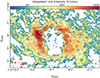 |
Fig. 1. CO(2–1) velocity-integrated map in units of Kelvin kilometers per second (K km s−1) obtained with ALMA in the CND of NGC 1068. The color ranges from the minimum to the maximum value in the logarithmic scale, and the contour covers the same extent with levels 3σ, 5σ, 10σ, 20σ, 40σ, 60σ, 100σ–250σ in steps of 50σ, where 1σ = 50.6 K km s−1. Here, the 1σ value differs slightly from García-Burillo et al. (2019). We integrated over all channels instead of restricting to a certain range around vsys, which does not affect the velocity-integrated maps (this also applies to the CO(3–2) and CO(6–5) transitions, in comparison to García-Burillo et al. 2016). The smallest common beam size is indicated at the lower left corner of the figure, along with a linear scale indicator of 40 pc. The AGN position is also specified with two dashed lines. |
We also reproduced smoothed and regrided velocity-width maps in full width half maximum (FWHM) with the common resolution (Fig. 2 for the CO(2–1) transition as well as Figs. A.3 and A.4 in Appendix A for the CO(3–2) and CO(6–5) transitions respectively) based on García-Burillo et al. (2019), using 3σ clipping, to investigate molecular line widths throughout the CND.
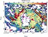 |
Fig. 2. CO(2–1) velocity-width map of the CND in units of FWHM. The color scale spans the range [20, 200] km s−1, and the contours traverse the same range with a step size of 30 km s−1. The magenta lines trace the borders of the previously constructed AGN wind bicone (Das et al. 2006). The remaining markers and symbols are the same as in Fig. 1. |
We likewise reproduced the smoothed and regrided residual mean velocity map from García-Burillo et al. (2019) with the common resolution for all CO transitions (Fig. 3 for the CO(2–1) transition as well as Figs. A.5 and A.6 in Appendix A for the CO(3–2) and the CO(6–5) transitions respectively) after 3σ clipping.
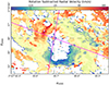 |
Fig. 3. CO(2–1) residual mean velocity field of the CND after the subtraction of projected CND rotation curve produced by García-Burillo et al. (2019). The color scale is within the range [−200, 200] km s−1 relative to the mean motion of the galaxy, vsys = 1120 km s−1, which is set to 0 km s−1. Blue (red) contours span from −200 (+50) to −50 (+200) km s−1 with a spacing of 25 km s−1 relative to vsys. The symbols and markers are the same as in Fig. 2. |
3.2. Region selections based on outflow goemetry
In order to investigate the locations of molecular gas dynamically affected by the kinematics of the AGN wind and the radio jet in detail, we selected regions across the CND (Fig. 4). The coordinates of these sampled regions are displayed in Table 2. Despite the high spatial resolution of our data, ∼0.1″ corresponding to a linear scale of 7 pc, we used squared regions with a linear size of 40 pc, matching an angular size of ∼0.57″, due to the high variance of physical behaviors across adjacent regions at smaller scales. We also defined these regions based on the AGN wind bicone (Das et al. 2006), where the green-colored regions are situated either within the bicone or along the edge of the model, while the orange regions are completely outside the bicone. These regions were also sampled close to the inner edge of the CND, supposedly under more influence from the ionized outflow from the central engine compared to the CND outskirt. To prevent mixing up different regions defined across the CND, we adopted a naming scheme of the form “inside/outside bicone (in color)” + “region number” + “_size” + “(position inside the CND)” (e.g., G1_40 (N) for green region 1 inside or along the edge of the AGN bicone in the northern CND and O2_40 (W) for orange region 2 outside the bicone in the western CND). These regions (see Table 2) were used for the physical and kinematics interpretation of molecular gas inside the CND, as shown in the following sections.
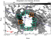 |
Fig. 4. Region selection based on the AGN wind bicone indicated by the purple lines. The green regions are located either within the bicone or along the edge of the bicone, while the orange regions are outside the bicone. The numbers marked within each region match those in region codes displayed in Table 2 and are defined in Sect. 3.2. The background plot, including markers and symbols, is the de-colored CO(2–1) velocity-integrated map from Fig. 1. |
Coordinates of regions sampled based on outflow.
4. Physical properties of the CND
In this section, we construct a temperature and density map of the CO gas, assuming LTE conditions. Knowledge of the temperature and excitation conditions could help discern between gas swept by the outflow and gas with a high temperature, which might indicate whether the outflowing gas in the northeastern part of the CND is being dynamically influenced by the ionized AGN wind.
4.1. LTE analysis
Assuming optically thin LTE conditions, we quantitatively estimated the total gas column densities with
where Z=kTk/hBrot is the partition function (Brot is the rotational constant of CO, and h is the Planck constant); k is the Boltzmann constant; gu is the statistical weight of the upper-level u; Eu is the energy of the upper-level u; Tk=Trot is the kinetic temperature of the gas, which is equal to the rotational temperature if all levels are thermalized; and

is the column density of level u. Here, ν is the transition frequency, I is the integrated line intensity in units of K km s−1, and Aul is the Einstein A coefficient for transitions from upper level u to lower level l. When calculating I for each of the 40 × 40 pc regions defined in Sect. 3.2 for each CO transition, we averaged only over available values within each region, ignoring pixels without detected emission (eliminated by 3σ clipping). The effective area filling factor is thus the fraction of the region covered by remaining emissions1. By calculating the total column densities, one can also estimate the rotational temperatures based on rotational diagrams of upper-level column densities from three CO transitions as an intermediate step, which relates the level column densities per statistical weight to the upper-level energy above ground state. If the LTE condition is satisfied, the gas level populations (i.e., nu and nl for the upper and lower-level number densities) follow that of the Boltzmann distribution,
which simplifies to a linear relation (y=ax),
where the left-hand side is the difference in y (δy) and the right-hand side is the difference in x (δx=Eul/k) multiplied by the slop (−1/Tkin). As a result, the rotational temperature is associated with the fit slope, a, of a natural logarithmic rotational diagram through Trot∼Tkin=−1/a. While, in reality, it is unlikely that all the gas is in the LTE condition, total CO column densities and rotational temperatures derived following the formulations above can be instructive in providing lower limits on the actual column densities and actual kinetic temperatures of the gas.
Following the above process, we first computed rotational temperatures for all the sampled regions by fitting the rotational diagrams. For calculating the column densities, the partition function was computed by fitting the available data from CDMS (The Cologne Database for Molecular Spectroscopy) before assigning the corresponding rotational temperature to the fit function (Goorvitch 1994; Gendriesch et al. 2009). The total column densities were then calculated using the upper-level column density, the partition function, the rotational temperature, and the upper-level energy (also taken from CDMS) of each transition for each region. The error bars for column densities and rotational temperatures were propagated after assuming a 10% calibration error combined with the RMS uncertainty on integrated line intensities.
We produced rotational diagrams to visualize rotational temperatures and LTE conditions directly across the CND (see Fig. 5). All regions defined based on outflow display well-fit LTE models to the weighted upper-level column densities. Hence, gas within regions defined based on the outflow might be optically thin and in the LTE condition.
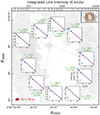 |
Fig. 5. Rotational diagrams of all regions defined based on the outflow occupying the same locations on the background plot as assigned in the region definition in Sect. 3.2. Region numbers are listed in Table 2. The y-axis of the rotational diagrams is in the natural logarithmic scale (contrary to the “log10” scale used in some other literature), while the x-axis is in the linear scale, and their labels are showcased for region G6_40 (S). The blue data points with error bars within each plot are the weighted upper-level column densities from three CO transitions at their respective upper energy levels. The purple dashed line and the corresponding light purple shaded area are the fit based on the LTE condition and its uncertainty. The calculated rotational temperatures and their uncertainties are in green. The background plot is a cutout from Fig. 1, and the cutout region is indicated in brown in the inset plot at the upper-right corner. The AGN wind bicone was added as shaded solid purple lines in the background plot, and the sampled region size is indicated at the lower-left corner. All the other symbols and markers of the background plot are the same as Fig. 1. |
A similar conclusion can be drawn from the average total column density values (see Table 3 and Fig. 6). We observe that for all regions defined based on the outflow, all three column densities calculated independently from three CO transitions roughly match the same level within each region. Column densities also vary across different regions. For regions sampled based on outflow, G1_40 (N) has the highest column density and is higher than column densities from other regions by a factor of ∼4. This region resides at the location with the highest integrated line intensity near the eastern knot (E-knot; see García-Burillo et al. 2019 and references therein), as seen from velocity-integrated maps.
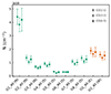 |
Fig. 6. Total CO column densities (N) independently calculated from three CO transitions for all regions selected based on the outflow. The x-axis marks the region labels along with their locations around the CND (in brackets), while the y-axis indicates the total CO column densities in the unit of cm−2. The region code (along the x-axis) and color (the color of the data points) of each region match those in Table 2 and are defined in Sect. 3.2. The legend at the upper-right corner of the plot designates the symbols corresponding to the column densities calculated from three different CO transitions. |
Rotational temperatures and total CO column densities from CO gas in 40×40 pc regions defined based on outflow.
We also summarize rotational temperatures in Table 3 and Fig. 7. Overall, our rotation temperature results at different positions of the CND roughly match with lower resolution results from Viti et al. (2014). The highest rotational temperature is at G1_40 (N), corresponding to its high CO column density and high integrated line intensity, and, in general, rotational temperatures in the northern part of the CND are higher than the southern part of the CND, possibly indicating higher excitation due to the proximity of the molecular gas to the central engine2. However, the difference between rotational temperature values in the northern and southern regions of the CND is not significant. In contrast, from Fig. 2, the difference in velocity widths between the northeastern and the southern parts of the CND are considerable. This difference likely reflects the dynamic asymmetry of the molecular outflow. Specifically, the molecular gas in the northeastern CND appears to offer greater resistance to the ionized AGN wind or the radio jet, whereas the molecular gas in the southern CND has largely been dissociated. In fact, the morphology of the radio jet nebula imaged by the Very Large Array (VLA) at cm wavelengths (Gallimore et al. 1996) and by ALMA at mm wavelengths (García-Burillo et al. 2017) exhibits a pronounced northeast-to-south asymmetry. The northeastern radio lobe displays a distinct bow-shock arc structure and spans a smaller radial distance from the AGN compared to the southern radio lobe, which has a broader angle shape. These observations suggest that the radio jet in the southern CND is more evolved, indicating extensive past destruction of molecular gas in the southern CND.
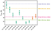 |
Fig. 7. Summary of rotational temperatures for all regions sampled around the CND defined based on the outflow in Sect. 3.2. The x-axis marks the region labels along with their locations around the CND (in brackets), while the y-axis indicates the rotational temperatures in the unit of K. The region code (along the x-axis) and color (the color of the data points) of each region match those in Table 2 and are defined in Sect. 3.2. The purple, yellow, pink, and lime dashed lines indicate the rotational temperatures at four different locations of the CND measured by Viti et al. (2014). |
4.2. Non-LTE analysis
To validate the well-fit rotational diagrams and the matching column densities indicating the LTE condition of regions defined based on the outflow, we ran simple RADEX analyses (van der Tak et al. 2007) with the Large Velocity Gradient (LVG) method for each region using calculated rotational temperatures in the unit of K and total CO column densities in the unit of cm−2 to estimate corresponding optical depths, τ, for all CO transitions for all regions (see Table 4). We also calculated the line width spatially averaged within each region in FWHM and in the unit of km s−1 as an input parameter. For the total H2 density (the density of the major collision partner; nH2), we set up a grid of density values, nH2 = 104 cm−3, nH2 = 105 cm−3, and nH2 = 106 cm−3. Afterwards, we restricted the density values based on results from Table 6 in Viti et al. (2014). While most of the transitions for most regions result in τ<1, some of the regions near the E-knot, the W-knot, and CND-S display τ≳1, especially for a nH2 = 104 cm−3. However, as calculated with a RADEX grid search in Viti et al. (2014) using different line ratios of transitions from several available molecules, a nH2 = 104 cm−3 is unlikely within the CND, which leaves four regions with τ≳1, regions G1_40 (N), G7_40 (S), O1_40 (E), and O2_40 (W). For region G1_40 (N), optical depths calculated from the CO(3–2) and the CO(6–5) transitions with both nH2 = 105 cm−3 and nH2 = 106 cm−3 are slightly higher than 1 but below 1.5. For regions O1_40 (E) and O2_40 (W), only optical depths calculated from the CO(3–2) transition with both nH2 = 105 cm−3 and nH2 = 106 cm−3 are slightly higher than 1 but below 1.5. For region G7_40 (S), only the optical depth calculated from the CO(3–2) transition with nH2 = 105 cm−3 is at ∼1.1. Regardless, the opacity of the majority of gas within the CND is low and roughly matches the LTE condition.
Optical depth values of CO gas in 40×40 pc regions defined based on the outflow.
4.3. Line ratios
Previous studies using lower spatial resolution data (0.5″) have shown that individual molecular line ratios are correlated with the UV and X-ray illumination of the molecular gas in the CND from the central engine which can be used to infer certain physical conditions of the molecular outflow, especially the excitation conditions of the gas (García-Burillo et al. 2014; Viti et al. 2014). We therefore computed the CO(3–2)/(2–1), CO(6–5)/(2–1), and CO(6–5)/(3–2) ratio maps (Fig. B.1), using velocity-integrated intensity maps, to investigate the physical conditions of the CND. In general, due to a lack of emission of the CO(6–5) transition in the outer part of the CND, the inner CND has higher excitation compared to the outer CND. Within detected regions of the CND, the line ratios are higher in the northeast compared to the south, especially for the positions close to the northern and eastern inner edges of the structure. For the CO(3–2)/(2–1) ratio map, high excitation can also be spotted across the northeastern outskirt of the CND, further away from the central engine, as well as at a small section, located around α2000 = 2h42m40.63s and δ2000=−0°00′50″, along the southern outer edge of the CND. For CO(6–5)/(2–1) and CO(6–5)/(3–2) ratio maps, high ratios also appear along the southern outer edge of the CND and around the northern outskirt of the structure. Again, higher ratios around the northeastern part of the CND when compared to the southern part of the CND might be a result of the proximity of the northeastern CND to the central engine.
4.3.1. Region selections based on excitation
Besides selecting regions based on the outflow (see Sect. 3.2), we also sampled regions based on excitation using the ratio maps (see Fig. B.2 and Table B.1). We separated the regions based on excitation levels relative to the root-mean-square (RMS) values from each ratio map. The dashed regions contain line ratios higher than 3 times the RMS value, while the solid regions contain ratios exceeding 2 times the RMS value. In the case of the CO(6–5)/(3–2) ratio, no region with ratios higher than 3 times the RMS value was found. Again, the green and orange colors indicate the location of each region with respect to the AGN wind bicone model, as discussed in Sect. 3.2. We adopted a slightly different scheme for region definitions based on excitation in the form of “high ratio” + “inside/outside bicone (in color)” + “region number” + “_size” + “_ratio” (e.g., HRG1_40_3221 for region 1 inside or along the edge of the AGN wind bicone with high CO(3–2)/(2–1) ratio above 3 times the RMS value and HRO2_40_6532 for region 2 outside the bicone with high CO(6–5)/(3–2) ratio above 2 times the RMS value)3.
4.3.2. LTE analysis for high ratio regions
We likewise conducted the LTE analysis for gas within these high-excitation regions. Rotational diagrams indicate that LTE fits are worse for several regions sampled via high ratios than regions based on the outflow (see Fig. B.3), which means some gas within high ratio regions does not satisfy LTE conditions. We also found departures from LTE conditions based on the total CO column density values calculated independently using the 3 CO transitions (see Table B.1 and Fig. B.4), especially for region HRG3_40_3221, where the column density can only be interpreted as its lower limit. For ratios associated with the CO(6–5) transition, larger discrepancies among 3 column densities were found in the northern regions compared to the southern regions. The departure from LTE conditions might imply that (i) the gas is optically thick and/or (ii) multiple gas components are enclosed within each region. Hence, rotational temperature values of these regions can only be interpreted as lower limits of their gas kinetic temperatures.
Variations of column densities and rotational temperatures (see Table B.1 and Figs. B.4, B.5) among different regions are also evident for regions selected based on excitation. Region HRG3_40_3221 has column density roughly 6 times higher than other regions with the same definition. The same region also has about 2 times higher rotational temperature when compared to regions further away from the central engine (HRG1_40_3221 and HRG5_40_3221), which might not be as dynamically or radiatively affected. For regions with high excitation in CO(6–5)/(2–1) and CO(6–5)/(3–2) ratios, their column densities are approximately at the same level, while, overall, the northern regions outside the AGN wind bicone have higher rotational temperatures than in the southern regions inside the bicone.
5. Kinematics of the CND
Despite the CO gas being nearly in LTE across the CND, the average residual line profiles of several regions, as is shown in this section, imply multiple gas components. We shall now investigate the kinematics of the CO gas in order to determine the influence of the ionized outflow on the molecular CND and the extent of the outflowing molecular gas. Kinematics analyses around the central engine of NGC 1068 have been carried out previously by multiple studies (García-Burillo et al. 2016, 2019; Imanishi et al. 2020; Impellizzeri et al. 2019). While (Imanishi et al. 2020) and Impellizzeri et al. (2019) focus on kinematics of the torus (García-Burillo et al. 2016, 2019) studied kinematics of the CND using position-velocity diagrams and kinematics models. In this section, we introduce the line profile analysis to systematically probe the kinematics of molecular gas in detail using the spectral information of the CO observations for all regions defined in Sect. 3.2 based on the outflow.
5.1. Single versus multi-component Gaussian models
We performed rotation curve subtraction, using the rotation curve from García-Burillo et al. (2019), on the original data from three CO line observations without clipping. The rotation curve was fit based on the mean velocity distribution covering the central region of the galaxy in the CND coordinates of NGC 1068. We first projected the rotation curve to sky coordinates. After conversion to brightness temperature in units of K km s−1, emissions across all channels in three sets of CO observations were shifted to various velocities using the projected rotation map. We then spatially averaged emissions within each region defined based on the outflow while retaining the spectral dimension.
To systematize the line profile analysis, we adopted a similar technique as Imanishi et al. (2020) and fit all the averaged line profiles using three different models, a single Gaussian, a weighted double Gaussian, and a weighted triple Gaussian model:
![$$ S_{\nu }(v) = \begin {cases}A{\cal {{G}}}(\mu , \sigma ) = \frac {A}{\sqrt {2\pi }\sigma }e^{-\frac {(v-\mu )^2}{2\sigma ^2}} & ({\textrm {single}}) \\ A\left [w_1{\cal {{G}}}(\mu _1,\sigma _1)+w_2{\cal {{G}}}(\mu _2, \sigma _2)\right ] & ({\textrm {double}}) \\ A\left [w_1{\cal {{G}}}(\mu _1,\sigma _1)+w_2{\cal {{G}}}(\mu _2, \sigma _2)+w_3{\cal {{G}}}(\mu _3,\sigma _3)\right ] & ({\textrm {triple}})\,. \end {cases} $$](/articles/aa/full_html/2025/06/aa53704-25/aa53704-25-eq8.gif)
We found that in some spectra, the secondary component of the weighted double and triple Gaussian models has a limited contribution to the overall fit. Hence, we first eliminated all emissions below 3 times the background noise level from all line profiles so that the background noise does not influence the fitting results. Afterward, we employed a hierarchical scheme to choose the optimal model based on the fit. The fit double Gaussian model was first compared with the fit single Gaussian model using two criteria. For the first criterion, we applied the extra-sum-of-squares F-test (Lupton 1993) similar to Sexton et al. (2021) and Kovačević-Dojčinović et al. (2022). This test assumes a null hypothesis that a simpler model with fewer parameters (e.g., the single Gaussian model) is more effective at describing the averaged line profile than a more complex model with more parameters (e.g., the weighted double Gaussian model). The test was done for all the regions that passed the first criterion, and we retained all the weighted double Gaussian fit when the P-value <0.05. To prevent overfitting the line profiles, we also applied the Akaike information criterion (Akaike 1973),  , where k is the number of free parameters and
  is the likelihood of the line profile data given the fit, to restrict the more complex model based on its complexity (i.e., the number of parameters). The difference ΔAIC=AICsingle−AICdouble between the fitting results of the two models measures the degree to which the weighted double Gaussian is favored over the single Gaussian fit. Following (Wei et al. 2016), the weighted double Gaussian fit is considered “positive” when ΔAIC>2. When a weighted double Gaussian fit was rejected, the corresponding weighted triple Gaussian fit was also discarded. The same process was used to compare the remaining weighted double and triple Gaussian models.
5.2. Line profile behaviors
The line profiles and their optimal fits for each region sampled based on the outflow are shown in Figs. 8, 9, and 10, and their fit results, including parameter values, are displayed in Table C.14. We describe and discuss these line profile results in this section by separating them into different groups based on their behaviors and positions relative to the AGN wind bicone. When discussing a multi-component Gaussian fit, we define the first (major), secondary (minor), and third Gaussian components based on their weight parameters. Without the weight parameter, all Gaussian components are normalized based on the line profile. As a result, each Gaussian component captures the fraction of gas enclosed in each region proportional to the weight parameter.
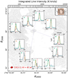 |
Fig. 8. CO(2–1) transition line profiles of all regions defined based on the outflow occupying the exact locations on the background plot as assigned in the region definition in Sect. 3.2. Region numbers, including their colors, are indicated at the upper-left corner of each plot. They correspond to those appearing in the region codes in Table 2 and are defined in Sect. 3.2. The x-axis of all line profile plots indicates the radial velocity of the gas, v, in the unit of km s−1. The y-axes are for the amount of emission within each channel, TB, in the unit of K. The blue data points and error bars within each region are the observed averaged line profile overplotted by the optimal fit as a green dashed line. The mean velocity of the galaxy, vsys, is indicated by the vertical red dash line for each line profile plot. Suppose the averaged line profile within one region was fit with a weighted multi-component Gaussian. All weighted Gaussian components are also provided in the plot as dotted lines using different colors (purple and orange for the first two components and brown for the third component). The transition of the line, CO(2–1), is indicated at the lower left corner of the background plot, and all other symbols are the same in the background plot as those in Fig. 5. |
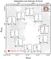 |
Fig. 9. CO(3–2) transition line profiles of all regions defined based on the outflow occupying the exact locations on the background plot as assigned in the region definition in Sect. 3.2. The background plot is the CO(3–2) velocity-integrated map from Fig. A.1. The transition of the line CO(3–2) is indicated at the lower left corner of the background plot. All other symbols and markers are the same as Fig. 8. |
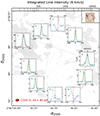 |
Fig. 10. CO(6–5) transition line profiles of all regions defined based on the outflow occupying the exact locations on the background plot as assigned in the region definition in Sect. 3.2. The background plot is the CO(6–5) velocity-integrated map from Fig. A.2. The transition of the line CO(6–5) is indicated at the lower left corner of the background plot. All other symbols and markers are the same as Fig. 8. |
5.2.1. Regions G1_40 (N) and G2_40 (N)
Regions G1_40 (N) and G2_40 (N) (inset plots in the upper-left corners of Figs. 8, 9, and 10) are located in the northeastern part of the CND, along and within the AGN wind bicone. In region G1_40 (N), the emission line profiles for all three CO transitions–CO(2–1), CO(3–2), and CO(6–5)–roughly overlap in velocity space, with their bulk emission consistently appearing above the galaxy's systematic velocity at vsys = 1120 km s−1, as indicated by the red dashed lines in the figures. For all transitions, the two Gaussian components have peaks above vsys. The primary components, although closer to the mean velocity, remain redshifted by ≳30 km s−1 from vsys, and a spectral resolution of 20 km s−1 (channel width) is sufficient to confirm this departure. The CO(6–5) transition line profile in this region exhibits large error bars on fit parameters, potentially diverging from the results of other transitions. However, the CO(6–5) line profile shows an enhanced redshifted wing structure consistent with the CO(2–1) and CO(3–2) profiles. Similar patterns are evident in the fitting results for region G2_40 (N), where the CO(2–1) and CO(3–2) transitions exhibit comparable redshifted features. In contrast, the CO(6–5) transition in this region is fit with only a single redshifted Gaussian. Additionally, for region G2_40 (N), the primary component of the CO(2–1) line profile is more significantly redshifted from the systematic velocity than its secondary component.
Several trends can be inferred from the line profiles in regions G1_40 (N) and G2_40 (N). Most of the gas in these regions is redshifted, with an additional redshifted wing structure characteristic of outflow dynamics. Notably, in both regions, the wing components (characterized by the widths of the fit Gaussian profiles) exhibit broader widths than their corresponding components with smaller velocity departures. These broad-wing components likely trace the molecular outflow at the interface where the ionized AGN wind interacts with the molecular gas at the surface of the CND facing the observer. In contrast, the less redshifted components likely correspond to gas embedded deeper within the CND, dynamically influenced by the outflow but less directly exposed. Across transitions, as indicated by the weight parameters, the wing components of the CO(2–1) transition are the most prominent in both regions, while the less redshifted Gaussian components are generally stronger in higher-J transitions compared to lower-J transitions. These observations suggest that the gas associated with the wing component may be less dense than the gas corresponding to the lower-velocity component.
5.2.2. Region G3_40 (N)
Region G3_40 (N), located along the northwestern edge of the AGN wind bicone, exhibits simpler line profile behavior compared to the more complex profiles seen in the northeastern regions G1_40 (N) and G2_40 (N). The CO(2–1) transition is well-described by a single Gaussian, with its mean velocity redshifted by less than one channel width from vsys. The width of this single Gaussian profile is also narrower than the wing components observed in regions G1_40 (N) and G2_40 (N). In contrast, the CO(3–2) line profile is best fit with a double Gaussian, consisting of a redshifted primary component and a slightly blueshifted secondary component. The primary component likely traces gas at the edge of the molecular outflow, while the secondary component may represent gas outside the AGN wind bicone, dynamically independent from the outflow. For the CO(6–5) transition, no significant detection was observed, as the maximum or minimum value of the line profile remains below the 3σ noise threshold.
A spatial variation of line profiles is evident among the three northern regions, particularly highlighted by the differences between region G3_40 (N) and the other two regions. The gas in region G3_40 (N) aligns more closely with the galaxy's systematic velocity and appears less influenced by the outflow, as indicated by the CO(2–1) and CO(3–2) line profiles. This is consistent with a significant portion of the region lying outside the AGN wind bicone and its location at the edge of the line broadening and redshifted rotation-subtracted radial velocity features previously shown in Figs. 2 and 3. In contrast, region G2_40 (N), positioned near the center of the ionized AGN wind bicone, captures a more substantial amount of molecular outflow than region G3_40 (N). Meanwhile, despite being located at the edge of the bicone, region G1_40 (N), which coincides with line broadening and redshifted rotation-subtracted radial velocity features, also contains a considerable amount of outflowing molecular gas.
5.2.3. Regions G4_40 (S), G5_40 (S), and G6_40 (S)
The line profile behaviors in the southeastern part of the CND differ significantly from those in the northeastern regions. In all three southeastern regions, the CO(2–1) and CO(3–2) transitions exhibit similar line profile characteristics. For the CO(3–2) transition, the profiles are modeled using double Gaussians, with the primary components blueshifted by more than 120 km s−1 below vsys. The secondary components are less blueshifted but remain ≳35 km s−1 away from vsys, exceeding one channel width. A similar trend is observed in the CO(2–1) line profiles of regions G4_40 (S) and G5_40 (S). In contrast, the CO(2–1) line profile of region G6_40 (S) is fit with a single Gaussian, but its peak is blueshifted by more than 140 km s−1. For the CO(6–5) transition, only the line profile from region G4_40 (S) is fit with a significantly blueshifted single Gaussian, while the emission from the other two regions is weak relative to the noise level. Additionally, in region G4_40 (S), a redshifted absorption feature is detected in the CO(2–1) line profile.
Contrary to the line profiles in the northeastern part of the CND, the secondary components of line profiles in regions G4_40 (S), G5_40 (S), and G6_40 (S) are either more closely aligned with the galaxy's mean motion relative to the primary components or are entirely absent. This distinction between the northeastern and southeastern regions suggests that the ionized outflow in the southeastern part of the CND may be significantly stronger than in the northeast. However, high-velocity wing components are absent in the southeastern line profiles, replaced by two well-separated components in regions G5_40 (S) and G6_40 (S), indicative of a multi-component molecular outflow5. Additionally, the widths of the more blueshifted components are comparable to those of the less blueshifted components in regions G4_40 (S) and G5_40 (S). Comparing the CO(3–2) line profiles from these regions, the line profile and its individual components exhibit the narrowest width in region G5_40 (S). The narrower width may reflect a weaker emission, potentially due to significant molecular gas dissociation caused by intense interactions with ionized outflows. Region G5_40 (S) appears to host the strongest ionized outflow among these regions, characterized by its high velocity and a relatively prominent, further blueshifted component. In fact, the farther blueshifted primary component of the CO(3–2) line profile is most prominent in region G5_40 (S), as indicated by the weight parameters. Notably, G5_40 (S) also roughly aligns with the southern molecular outflow direction identified by García-Burillo et al. (2019), which extends from the torus out into the CND.
5.2.4. Regions G7_40 (S) and G8_40 (S)
Similar to region G4_40 (S), the CO(6–5) transition line profile of region G7_40 (S) is best fit with a significantly blueshifted single Gaussian. In contrast, the CO(2–1) and CO(3–2) transition line profiles for region G7_40 (S) are modeled with double Gaussians. Unlike the southeastern regions, the two Gaussian components in region G7_40 (S) are closer in velocity. Specifically, the primary component of the CO(3–2) line profile may reflect the overall broadening of the emission line, while the corresponding minor component is offset by approximately 100 km s−1 below vsys. For the CO(2–1) line profile, the minor component corresponds to a blueshifted wing structure reminiscent of the redshifted wing components observed in the northeastern regions. In contrast, the CO(6–5) transition line profile in region G8_40 (S) is centered around vsys. For this region, while the bulk of the CO(2–1) and CO(3–2) line profiles is also centered around the galaxy's mean motion and appears independent of the outflow, both transitions feature two minor components blueshifted by more than 100 km s−1 from vsys, suggesting the presence of gas entrained in the outflow.
When comparing these two regions to the southeastern regions, a lateral trend becomes apparent. The blueshifted velocity departure of the bulk CO(2–1) transition line profile reaches its maximum in region G5_40 (S) and decreases, moving eastward toward region G4_40 (S) and westward toward region G8_40 (S). A similar trend is observed for the major component of the CO(3–2) transition line profiles, with its velocity departure and width both decreasing from region G5_40 (S) compared to regions G4_40 (S) and G7_40 (S). Overall, the outflow strength appears to peak near region G5_40 (S), but the amount of outflowing molecular gas decreases in this region, indicating a dynamic but less molecular gas-rich environment.
5.2.5. Regions O1_40 (E) and O2_40 (W)
All line profiles in the two regions outside the AGN wind bicone, O1_40 (E) and O2_40 (W), are well-fit with a single Gaussian centered around vsys, within one channel width. The broad widths of these profiles (≳200 km s−1) may suggest a lateral outflow driven by a hot cocoon of ionized gas caused by the expanding radio jet (Couto et al. 2017; Balmaverde et al. 2019; Venturi et al. 2021; Balmaverde et al. 2022).
5.2.6. Summary of line profile behaviors across the CND
In summary, the CO(2–1) and CO(3–2) transition line profiles provide a comprehensive view of the gas kinematics at various positions within the CND, whereas the CO(6–5) transition often lacks sufficient emission to provide kinematic information for several regions. Overall, the majority of line profiles in the northeastern regions exhibit predominantly redshifted features with stronger emissions, while those in the southern regions are primarily blueshifted with comparatively weaker emissions, aligning with the gas dynamics illustrated in Figs. 1 and 3. As shown in Fig. 11, the line-of-sight velocity departure of molecular gas within the outflow is larger in the southern part of the CND compared to the northern part. This, combined with the relative depletion of CO, suggests a stronger ionized outflow in the southern CND, potentially due to an outflow geometry where the southern AGN wind lies closer to the CND plane than the northern AGN wind. In the southern regions, molecular gas embedded deeper within the CND may be more strongly influenced by the ionized outflow. In particular, under the stronger outflow between regions G4_40 (S) and G6_40 (S), the high-velocity components from double Gaussian fits are more prominent, as indicated by larger weight parameters for these components compared to their corresponding low-velocity components in the southern CND. Spatial variations are also evident across regions within or along the AGN wind bicone. In the southern half of the bicone, the more blueshifted component is most prominent in region G5_40 (S), with its prominence decreasing toward region G8_40 (S) to the west and region G4_40 (S) to the east. In the northern half, the wing components of line profiles are broader and more redshifted in region G1_40 (N) than in G2_40 (N) (also see Fig. 12), while the wing component disappears entirely in region G3_40 (N). These broad-wing structures indicate that molecular gas at the surface of the CND is being swept by the ionized AGN wind. Furthermore, in most regions with detectable outflows, low-velocity components (see the left and mid panels of Fig. 11) are also significantly shifted from the galaxy's systematic velocity, revealing multi-component outflows within the CND. In contrast, regions outside the AGN wind bicone show broad single-component emissions centered at the mean velocity of the galaxy, potentially implying influence from a jet-induced lateral outflow.
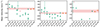 |
Fig. 11. Mean velocity values of all Gaussian components fit to the line profiles for the CO(2–1) (left panel), the CO(3–2) (mid panel), and the CO(6–5) (right panel) transitions on the scale of 40×40 pc. For each panel, the red shaded region marks ± one channel width away from the systematic velocity of the galaxy, vsys. Based on the weight parameter, round symbols correspond to the largest component of each fit, the diamond symbols correspond to the secondary component of each fit, and the square symbols correspond to the smallest component of each fit. The downward triangle symbol indicates the Gaussian component for absorption, and the “×” symbol implies large error bars. All other schematics are the same as Fig. 6. |
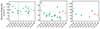 |
Fig. 12. Velocity dispersion values of all Gaussian components fit to the line profiles for the CO(2–1) (left panel), the CO(3–2) (mid panel), and the CO(6–5) (right panel) transitions on the scale of 40×40 pc. All schematics follow that of Fig. 11. |
We also examined the line profiles of regions defined based on excitation, which exhibit complex behaviors indicative of potential multiple gas components within each region. This complexity is consistent with the LTE analysis presented in Sect. 4.3. However, the intricate nature of these line profiles poses challenges for a detailed kinematic analysis, which is beyond the scope of this study.
5.3. Kinematics behavior at smaller scales
To (1) investigate the scale at which the multiplicity of gas components breaks down (i.e., the scale at which a region encompasses only one gas component) and (2) attempt to isolate the outflow material entirely, we first sampled smaller regions on a scale of 20×20 pc within each of the previously defined regions, centered at their midpoints (see descriptions in Appendix D.1). We then shifted these 20×20 pc regions to occupy different “corners” of their original 40×40 pc regions. The same line profile analysis procedure as described in Sect. 5.1 was adopted, and the definition of Gaussian components for multi-component fits follows that of Sect. 5.2. The results are presented in Figs. E.1–E.6 and in Tables E.1–E.2 in Appendix E.
5.3.1. Definition of zoomed-in and shifted regions
The discrepancies between smaller and larger regions mentioned in Appendix D.1 indicate the potential presence of multiple components of gas within some of the original 40×40 pc regions. To investigate these discrepancies further, we defined new regions by taking advantage of the high spatial resolution of the data, aiming to disentangle the different components of gas occupying distinct parts of the original 40×40 pc regions. For these new region definitions, we shifted the existing 20×20 pc regions, with the adjustments varying across different regions. For positions G1 and G2, the 20×20 pc regions were shifted to the lower right (designated as DR) corners of the corresponding 40×40 pc regions to potentially capture stronger outflow signatures closer to the central engine. For position G7, a new 20×20 pc region was created to occupy the upper left (designated as UL) corner of G7_40 (S), aiming to include stronger outflow along the inner edge of the CND. At position G8, located along the edge of the bicone, the new 20×20 pc region was selected to occupy the lower left (designated as DL) corner of G8_40 (S), contrasting with position G4, where the 20×20 pc region was shifted to cover the entire lower right (DR) corner of G4_40 (S). For the southern positions G5 and G6, the new 20×20 pc regions were chosen further from the AGN position to potentially capture less gas entrained in strong outflows. For G5, the 20×20 pc region was shifted to occupy the lower (designated as D) part of G5_40 (S), centered at the right ascension coordinate of the original region, while for G6, the lower right (DR) corner was selected. Returning to the northern CND, for region G3_40 (N), most of which lies outside the AGN wind bicone, the 20×20 pc region was shifted to the eastern part of G3_40 (N), centered on its declination coordinate, to search for outflow signatures while avoiding the upper left corner, which lacks CO(6–5) emission. Additionally, since a significant fraction of G4_40 (S) with a prominent highly blueshifted Gaussian component lies outside the AGN wind bicone, we also sampled the lower right corner (DR) of region O1_40 (E) as a zoomed-in and shifted region. A shifted region was not defined for position O2 outside the bicone. The naming scheme for the new regions includes the position code, the size of the region, and the direction of the shift (e.g., for a 20×20 pc region occupying the lower right corner of G1_40 (N), the region code is G1_20_DR (N)).
5.3.2. Kinematics of zoomed-in and shifted regions
Line profiles and their optimal fits of the shifted regions are shown in Fig. E.2 for the CO(2–1) transition, Fig. E.4 for the CO(3–2) transition, and Fig. E.6 for the CO(6–5) transition. A summary of the fitting results is displayed in Table E.2. Detailed descriptions of the behavior of these line profiles can be found in Appendix D.2.
Based on line profiles of the zoomed-in and shifted regions (see descriptions in Appendix D.2), more molecular gas is entrained in the outflow closer to or inside the AGN wind bicone. In the southern CND, the ionized outflow is stronger along the inner edge of the CND, which causes more molecular gas to be entrained in the high-velocity component of the outflow. In the northeastern CND, the ionized outflow is stronger further away from the inner edge of the CND, characterized by broad wing components within the line profiles. One possible explanation for the different line profile behaviors in the northern and southern CND is the 3D outflow geometry (García-Burillo et al. 2019; see Fig. 13). The ionized outflow is closer to the plane of the CND in the south, where the ionized outflow contacts the inner edge of the CND first, than in the north, where the ionized outflow first contacts the top of the CND facing the observer away from the inner edge and sweeps the molecular gas at the surface of the CND. A substantial amount of molecular gas was also found extending outside the AGN wind bicone into the eastern part of the CND. Considering positions G1 and G5 might coincide with the strongest interactions between the molecular gas and the ionized outflow, a possible “misalignment” might exist between the ionized AGN wind bicone and the molecular outflow. This asymmetry of the molecular outflow also matches the structure of the radio jet previously observed in ionization bubbles by May & Steiner (2017).
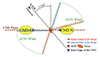 |
Fig. 13. Scheme of the narrow-line region in NGC 1068 (not to scale). The ionized AGN wind (green) is blueshifted (blue arrows) on the front face and redshifted (red arrows) on the back, as viewed along the line of sight. Interaction between the AGN wind and the CND (yellow ellipses) drives molecular outflows, blueshifted in the south and redshifted in the north, as observed by ALMA. The tilt of the AGN wind relative to the CND affects outflow locations: in the north, it interacts farther from the AGN than the inner edge (marked by purple crosses) of the CND, while in the south, interaction occurs at the inner edge. As a result, the strongest molecular outflows emerge at the inner edge of the southern CND and farther from the inner edge in the northern CND. |
5.4. Temperature and CO column density behaviors at smaller scales
In addition to the line profile investigation on the scale of 20×20 pc and for the shifted regions, as discussed in Sects. 5.3 and 5.3.2, we created rotational diagrams to check the LTE condition and temperature structure for these smaller regions. The results are shown in Figs. F.1 and F.2 and are displayed in Tables F.1 and F.2. Summaries of rotational temperatures and total CO column densities from all these regions are also provided in Figs. F.3 and F.4. Same as on the large 40×40 pc scale, gas within all smaller regions satisfies the LTE condition. Rotational temperatures from most of these regions also match with each other, and the values derived from gas within larger regions (within the error bar range), barring regions G3_20 (N), G5_40 (S), and all regions of position G6 in the southern CND. The inconsistency among the temperature values at the southern positions might be due to a stronger and multi-component outflow centered around position G5, while region G3_20 (N) might not contain as much outflowing gas with higher temperature as regions G3_40 (N) and G3_20_L (N). For the total CO column densities, their values from three transitions for each 20×20 pc or shifted region are consistent. The average CO column densities are slightly larger than those from the corresponding 40×40 pc regions but remain within the same order of magnitude. This increase in average column density may suggest a higher concentration of CO in the smaller regions. Overall, the density structure observed on the larger scale (as shown in Fig. 6) is preserved. Similar temperature and density behaviors observed across small and large scales may suggest that the clumpy CO gas within the CND is dynamically influenced by the ionized outflow. This interaction could lead to the stirring of molecular gas, promoting mixing and resulting in CO gas with low opacity. Optically thin CO emissions have been previously reported in similar systems, such as IC 5063 and NGC 3256-S, by Dasyra et al. (2016) and Pereira-Santaella et al. (2024).
6. Impact of the outflow
To understand the impact of the ionized outflow on the molecular gas inside the CND and the power of the molecular outflow, we calculated the mass outflow rate, dM/dt, for each 40×40 pc region defined based on the outflow (see Sect. 3.2) and compared the values between the northeastern and the southern CND. In this section, we first outline the method of estimating dM/dt values and follow it with a discussion on the implications of the mass outflow rate on the impact of the outflow across the CND.
6.1. Estimation of mass outflow rates
We first evaluate the total molecular mass impacted by the ionized outflow using the CO emission line brightness to molecular hydrogen column density conversion, XCO=N(H2)/ICO(1−0). Considering the low optical depth values calculated using RADEX in Sect. 4.1, in combination with relatively high excitation in the inner part of the CND (see Fig. 5), XCO inside the CND might be much lower than in the Milky Way or possibly lower than the value of  obtained in García-Burillo et al. (2014), where
  is the Milky Way value. A smaller XCO factor could imply a lower molecular mass within the outflow component of the CND. To calculate the average XCO values, we assume a range of CO abundances6, [CO]/[H2]∼5×10−5 to ∼10−4 (Usero et al. 2004). The values are computed based on XCO=NCO/([CO]/[H2] ICO(1−0)), and the ICO(1−0) values are extrapolated through rotational diagrams for each region. The results (see Table 5) are on average 4.8±0.4–9.6±0.9 times smaller than the canonical Milky Way value,
  , and are slightly lower than that of Usero et al. (2004), ∼4–8 times smaller than the canonical value. Regardless, the XCO values from this work are roughly consistent with values from Usero et al. (2004), García-Burillo et al. (2014), and Israel (2009a, b).
Estimated lower and upper XCO factors for 40×40 pc regions defined based on the outflow.
To derive the mass outflow rate, we need to assume a specific outflow geometry. Maiolino et al. (2012) and subsequently Cicone et al. (2014) provided two simple geometries of an AGN outflow, a conical/multi-conical outflow or a fragmented shell geometry, uniformly filled with outflowing clouds. Given that the 40×40 pc regions subtend a substantial radial span away from the AGN position (i.e., the “tip” of the outflowing cone), we adopted the fragmented shell geometry without approximation, and the mass outflow rate is given by
where vout is the average outflow speed of the region (velocity directs radially away from the AGN in the NGC 1068 galactic frame), Mout is the outflowing molecular mass, and rout and rin are the outer and inner radii of the shell.
The outflow mass, Mout, can be calculated from the residual CO image cubes (without rotation of the CND and mean motion of the galaxy). Following García-Burillo et al. (2014), all emission within 〈vres〉=[−50, +50] km s−1 was subtracted from residual CO image cubes to eliminate the contribution from non-outflowing gas with virial motions around the rotation (vres is the residual velocity of the gas excluding rotation and the mean motion of the galaxy). The resulting cubes containing mostly outflowing gas were applied 3σ clipping before being used to produce an outflow velocity-integrated map (see Figs. G.1, G.2, and G.3), which contains the total emission from the outflow across the CND. Ratios between the emission from the outflow and the total emission were then calculated. We ignored the ratios from the CO(6–5) transition due to a lack of detection in some regions. The average ratios were used to infer the amount of ICO(1−0) corresponding to the outflowing gas, ICO(1−0), out. In turn, ICO(1−0), out was used to evaluate N(H2)out, the average column density of outflowing gas within each region and, subsequently, Mout.
Similar to Mout, the outflow speed values, vout, were also estimated from the residual CO image cubes. After 3σ clipping, the resulting cubes were used for producing outflow radial-velocity fields for all transitions, which contain the mean line of sight velocity of the outflow, vLOS. To calculate vout, we need to de-project vLOS which can be considered as the line of sight component of the outflow velocity in the sky coordinates, vsky (see Fig. 14 for visualization). Likewise, vout can be considered as the radial component outward from the AGN position in the plane of the CND of the outflow velocity in the CND coordinates, vgal. When projecting vgal to vsky (i.e., from the CND coordinates to sky), two rotation matrices were applied to correct for the position angle and inclination,
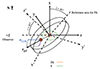 |
Fig. 14. Projection of velocity (vgal) from NGC 1068 coordinates (primed) to sky coordinates (unprimed). The primed frame results from a i = 41° inclination rotation along the line of sight (from the negative z-axis to the z′-axis) and a PA = 289° rotation around z′-axis. The x′-axis aligns with the minor axis of the CND, matching the reference azimuthal direction (θ′0), with the 90° difference between x′ and y′-axes corresponding to the difference between PA and the θ′0 direction. The primed system follows a rightward primary axis convention, while the sky frame follows a northward reference. The PA reference axis is the x-axis after inclination rotation. The brown ball marks the molecular gas region, with outflow velocity vgal assumed to lie in the CND plane, directed radially from the AGN (red star). It decomposes as voutcos(θ) along x′-axis and voutsin(θ) along y′-axis, where θ is measured from x′-axis. Using Eq. (8), vgal is projected to sky velocity vsky, decomposed into the observed radial velocity vLOS and a transverse component (purple arrow), which further splits into vx and vy. |
![$$ \begin{aligned} \boldsymbol {v}_{\mathrm {{sky}}} &= \boldsymbol {\mathbf {{R}}}_{\mathit {i}}\,\boldsymbol {\mathbf {{R}}}_{{\mathrm {PA}}}\,\boldsymbol {v}_{\mathrm {{gal}}} \\ &= \left [\begin {array}{ccc} \cos ({\mathrm {PA}}) & -\sin ({\mathrm {PA}}) & 0 \\ \cos (i)\sin ({\mathrm {PA}}) & \cos (i)\cos ({\mathrm {PA}}) & -\sin (i) \\ \sin (i)\sin ({\mathrm {PA}}) & \sin (i)\cos ({\mathrm {PA}}) & \cos (i) \\ \end {array}\right ] \,\boldsymbol {v}_{\mathrm {{gal}}}\,. \end{aligned} $$](/articles/aa/full_html/2025/06/aa53704-25/aa53704-25-eq15.gif)
Here, vgal is assumed to be completely contributed from the outflow (and inflow7), and
![$$ \boldsymbol {v}_{\mathrm {{gal}}} = \left [\begin {array}{c} v_{\mathrm {{out}}}\cos (\theta ) \\ v_{\mathrm {{out}}}\sin (\theta ) \\ v_{\perp }\sim 0 \\ \end {array}\right ], $$](/articles/aa/full_html/2025/06/aa53704-25/aa53704-25-eq16.gif)
where θ is the angle of the position of the gas with respect to the reference azimuthal direction in the CND coordinates, θ0′=PA−90° = 199° in the sky coordinates. We effectively assume that the outflow radially outward from the AGN position (or the inflow radially toward the AGN position) is the only velocity contributing to the residual velocity in the sky coordinates, vsky. We also assume that the main outflow velocity is within the plane of the CND, and vout≫v⊥, where v⊥ is the potential outflow velocity component perpendicular to the CND plane. Here, we note that vsky takes the form of
![$$ \boldsymbol {v}_{\mathrm {{sky}}} = \left [\begin {array}{c} v_{\mathrm {{x}}} \\ v_{\mathrm {{y}}} \\ v_{\mathrm {{LOS}}} \\ \end {array}\right ], $$](/articles/aa/full_html/2025/06/aa53704-25/aa53704-25-eq17.gif)
where vx and vy are contributions from the outflow to velocity perpendicular to the line of sight. By combining Eqs. (8)–(10), the relation between the outflow speed and the mean line of sight radial velocity can be expressed as
We first de-projected the entire line of sight velocity field to the outflow speed map for each transition. For this process, we set PA = 289° and i = 41°, following that of García-Burillo et al. (2019). To avoid extreme outflow rates caused by velocity outliers within each region, we retained only the inner 68% of outflow speed values for each region and CO transition before computing the average outflow speed. 1σ uncertainties of outflow speed values were obtained through bootstrapping the average outflow speed within 68% of all values for each region.
To determine rin and rout, we first projected galactic radii from the AGN position to the sky coordinates. The projected radii map was also “clipped” for each transition to account only for the radii of emission above 3σ level. Subsequently, we calculated the 68% percentiles of radii within each region as rin and rout. Error bars of rin and rout were also computed via bootstrapping.
6.2. Mass outflow rates and outflow velocities across the CND
Following the recipe outlined above, we calculated the upper and lower limits of the mass outflow rate for all regions and transitions based on the range of XCO for each region. Uncertainties of all outflow rate values were propagated from associated variables. The results are recorded in Table 6. We also display average outflow speeds for each region and transition in Table 7.
Estimated mass outflow rates for 40×40 pc regions defined based on the outflow.
Outflow speed away from the AGN position in the plane of the CND for 40×40 pc regions defined based on the outflow.
Region G1_40 (N) (see Fig. 4) has a significantly larger molecular mass outflow rate compared to other regions, which reveals that the mass outflow rate mainly depends on the total enclosed mass of molecular gas within each region. Considering the numerical difference between rin and rout is much larger than vout, the remainder of Eq. (7) is substantially smaller than the values of Mout, which are in the order of ∼105 (mainly in the southern CND) to ∼106 M⊙ (mainly in the northeastern CND)8, and Mout for each region is about ∼10–20 times smaller than the total outflowing molecular mass inside the CND,  (García-Burillo et al. 2014). A lower molecular mass budget in the southern CND than in the northeast indicates the depletion of molecular gas in the south, which contributes to the relatively low molecular mass outflow rates. When comparing outflow speed values between northern and southern regions, their values from regions G5_40 (S), G6_40 (S), and G7_40 (S) are larger than the two northern regions, G2_40 (N) and G3_40 (N). However, region G1_40 (N) in the northeast has the largest outflow speed, more than 2 times higher than that of the southern regions. Outside the AGN wind bicone, region O1_40 (E) exhibits a lower mass outflow rate compared to the southern regions, along with a low outflow speed below the virial speed of 50 km s−1, suggesting a limited impact from the outflow in this area. On the other side of the CND, region O2_40 (W) shows a negative mass outflow rate and a negative outflow speed of ≲50 km s−1, which could indicate an inflow of molecular gas. However, the negative outflow speed in this region may be an artifact introduced by the asymptotic behavior of the inverse sin function in Eq. (11).
We averaged molecular mass outflow rates among the northern and southern regions separately, excluding the CO(6–5) transitions of regions G3_40 (N), G5_40 (S), and G6_40 (S) due to a lack of detection. In the northeastern CND, the average outflow rate within a 40×40 pc region ranges from 8.5±1.5 to 17.0±3.0 M⊙ yr−1. These numbers decrease to 0.72±0.13–1.44±0.26 M⊙ yr−1 without region G1_40 (N). The average outflow rate in the southern CND is 1.35±0.14–2.71±0.29 M⊙ yr−1. The average outflow rate of the northeastern CND is higher than that of the southern CND, implying a stronger molecular outflow in the northeast, especially around region G1_40 (N). We likewise calculated the average outflow speed among the northern and southern regions. The average outflow speed in the northeast is 288.2±2.8 km s−1, and the average outflow speed in the south is 187.1±1.9 km s−1. If we exclude region G1_40 (N), the average outflow speed in the north drops to 70.4±1.0 km s−1. The substantial molecular gas reservoir near region G1_40 (N) appears to be more strongly influenced by the ionized outflow compared to the rest of the CND. This significant molecular mass outflow suggests a greater resistance to the ionized AGN wind in this area. Additionally, the outflow impacts a broader region in the southern CND than in the northeastern CND, where the molecular outflow is primarily concentrated around region G1_40 (N).
We further calculated the total molecular mass outflow rate of all regions, and the total amounts to 38.4±3.9 M⊙ yr−1, which is around 60% the value for the entire CND stated in García-Burillo et al. (2014),  . This fraction exceeds the ratio of the total sampled area to the geometrical extent of the CND. The discrepancy might be owing to different geometries used for the mass outflow rate calculation. While García-Burillo et al. (2014) adopted the conical model for a more conservative value, we decided to calculate more precise outflow rates for the comparisons between regions. Regardless, when following the approach using the conical model, the total outflow rate from all regions is 27.9±3.0 M⊙ yr−1, which counts about 45% of the mass outflow rate of the entire CND. Considering the physical scale of the CND is more than double that of the sampled regions combined, the majority of the molecular outflow power comes from the inner part of the CND, especially around region G1_40 (N).
7. Conclusions
We have selected a number of regions within the CND of NGC 1068 and investigated the temperature and density distribution of molecular gas within the CND using high spatial resolution (∼0.1″ or ∼7 pc) data from the CO(2–1), CO(3–2), and CO(6–5) transitions previously observed by ALMA. We characterized the kinematics of gas by analyzing residual line profile behaviors within the selected regions after subtracting rotation of the CND from the data. We also calculated corresponding molecular mass outflow rates and outflow speed values in the plane of the CND. Our conclusions are summarized as follows:
-
i
Most of the CO gas within the CND of NGC 1068 is optically thin and exhibits LTE conditions, as concluded from both the LTE and the RADEX analyses. Departures from LTE conditions are only observed for CO gas with high excitation, indicating either an optically thick condition or multiple gas components within these regions.
-
ii
The rotational (or kinetic) temperatures of CO across the CND match the lower resolution values reported by Viti et al. (2014) and range between ∼30 K and ∼60 K, with slightly higher temperatures (≳40 K) observed in the northeastern regions. In contrast, CO gas in the northeastern CND displays much broader line widths compared to the southern CND. This difference in line widths suggests a dynamic asymmetry between the northeastern and southern outflows, with the molecular gas in the northeast offering greater resistance to the ionized AGN wind.
-
iii
Line profiles from the 40 × 40 pc regions within or along the edge of the bicone display an increasing fraction of high-velocity outflowing molecular gas toward a position offset east of the southern bicone center from the southeastern and southwestern boundaries of the bicone, as well as toward the east from the west in the northern part of the bicone. These regions on the eastern side of the AGN wind bicone show a higher prevalence of high-velocity molecular outflows, suggesting a potential misalignment between the molecular and ionized outflows.
-
iv
Line profiles from further zoomed-in and shifted 20×20 pc regions outside or along the edge of the AGN wind bicone show an increasing fraction of outflowing molecular gas closer to or further inside the AGN wind bicone. A significant amount of outflowing molecular gas was also detected outside the AGN wind bicone in the eastern part of the CND, implying a mismatch in the spread between the molecular and ionized outflows.
-
v
From the zoomed-in and shifted 20×20 pc regions, we also observe a larger fraction of outflowing molecular gas near the inner edge of the CND in the south, contrary to a smaller fraction of outflowing molecular gas along the northern inner edge of the CND. This suggests that the ionized AGN wind may be tilted farther away from the plane of the CND in the northeast compared to the south.
-
vi
For regions inside the AGN wind bicone or along the eastern edge of the AGN wind bicone with line profiles fit with multi-Gaussian models, their low-velocity components are shifted more than one channel width (20 km s−1) away from vsys, indicating a multi-component molecular outflow.
-
vii
We calculated XCO values across the CND, and the values are 4.8±0.4–9.6±0.9 times smaller than the canonical Milky Way value,
 .
. -
viii
We calculated the molecular mass outflow rate and speed for regions within the CND by de-projecting line-of-sight velocities to outflow velocities in the plane of the CND and estimating the outflow molecular mass using XCO. The molecular mass outflow rate in region G1_40 (N) is significantly higher than in the rest of the CND. Outside region G1_40 (N), molecular mass outflow rates do not exceed ∼5.5 M⊙ yr−1 within each 40×40 pc region. This suggests that the ionized outflow has a minimal kinematic impact on the molecular gas reservoir in most of the CND.
-
ix
The total molecular mass outflow rate of all sampled regions within the CND exceeds 60% that of García-Burillo et al. (2014),
 , with region G1_40 (N) contributing to most of the outflow rate among these regions.
Our study further confirms the 3D outflow geometry proposed by García-Burillo et al. (2019) as a viable explanation for the outflow within the CND. This is supported by the observed asymmetry of the outflow. The ionized AGN wind appears to be located in front of the plane of the CND in the northeast, where it intersects with the molecular gas farther from the AGN position, near the geometrically thickest part of the structure. This interpretation aligns with a recent study by Hagiwara et al. (2024) on dense molecular gas (HCN and HCO+) and H2O maser spots within the streamer connecting the northern CND to the torus near component C of the 5 GHz continuum (see Gallimore et al. 1996, 2004). In the northeast, the ionized outflow may only sweep the surface of the molecular CND facing the observer, producing broad-wing structures in the line profiles observed in this region. Conversely, in the south, the ionized AGN wind seems to be angled closer to, but slightly behind, the plane of the CND, where it interacts with the molecular gas closer to the inner edge of the disc. The mass outflow rate is larger in the northeast, particularly near region G1_40 (N), indicating greater resistance from the molecular gas to the ionized outflow, especially when considering its high molecular gas density (Viti et al. 2014). This suggests the outflow in the northeast is less dynamically evolved compared to the south, as further evidenced by the asymmetric morphology of the radio jet (Gallimore et al. 1996). Beyond the E-knot, the impact of the ionized outflow on molecular gas is limited due to the predominantly optically thin nature of the CO gas within the CND. In these regions, especially in the southern CND, molecular gas dissociation reduces the kinematic influence of the ionized outflow.
Outside the AGN wind bicone, the origin of the broad line profiles is still unknown. Uncertainties remain regarding the molecular mass outflow rate and outflow speed in regions outside the bicone due to the simplified de-projection of line-of-sight velocity. The current velocity de-projection method does not account for motion outside the plane of the CND, potentially leading to inaccuracies. A more sophisticated kinematic model is required to address these limitations and could also provide a clearer explanation for the observed negative outflow rate in the western part of the CND.
Future ALMA observations might also benefit the understanding of molecular gas kinematics close to the AGN in NGC 1068. Despite the large variance in kinematic behaviors observed at small spatial scales (e.g., 20×20 pc), our study of the CND highlights the wealth of additional information that can be extracted using high spatial resolution data, particularly by comparing CO gas kinematics across different scales.
Data availability
The following materials supporting this article are available online: Appendices D–G (supporting texts, tables, and figures): https://doi.org/10.5281/zenodo.15147725; CO line profile movies: https://doi.org/10.5281/zenodo.15147919 and at https://www.aanda.org
Acknowledgments
We thank the anonymous referee for the useful suggestions for improving this paper. This project has received funding from the European Research Council (ERC) under the European Union's Horizon 2020 research and innovation programme (MOPPEX; Grant agreement No. 833460). YZZ, SV, and KYH acknowledge assistance from Allegro, the European ALMA Regional Center node in the Netherlands. This paper makes use of the following ALMA data: ADS/JAO.ALMA#2013.1.00055.S, ADS/JAO.ALMA#2016.1.00232.S. ALMA is a partnership of ESO (representing its member states), NSF (USA) and NINS (Japan), together with NRC (Canada), NSTC and ASIAA (Taiwan), and KASI (Republic of Korea), in cooperation with the Republic of Chile. The Joint ALMA Observatory is operated by ESO, AUI/NRAO and NAOJ. SGB acknowledges support from the Spanish grant PID2022-138560NB-I00, funded by MCIN/AEI/10.13039/501100011033/FEDER, EU. We acknowledge Louise Lamblin for her previous work on the project.
We note that the two regions O1_40 (E) and O2_40 (W) also have slightly higher temperatures relative to regions in the south despite being outside the bicone. The small temperature difference might be caused by the irradiation of molecular gas via high-energy photons/cosmic rays or ionized bubbles induced by the expanding radio jet.
Here, “region numbers” are used to distinguish high-excitation regions sampled under the same line ratio and are indicating different regions than in Sect. 3.2.
Movies showing the change of line profiles across the CND are available as online materials: https://doi.org/10.5281/zenodo.15147919
A small redshifted peak in some line profiles may represent the redshifted constituent of the molecular outflow, consistent with the 3D geometry described by García-Burillo et al. (2019). Less redshifted absorption features could arise from the foreground blueshifted outflow obscuring the background redshifted outflow. These features are not further analyzed due to low detectability.
References
- Aalto, S., Falstad, N., Muller, S., et al. 2020, A&A, 640, A104 [EDP Sciences] [Google Scholar]
- Akaike, H. 1973, in Second International Symposium on Information Theory, eds. B. N. Petrov, & F. Csáki (Budapest: Akadémiai Kiadó), 267 [Google Scholar]
- Alonso-Herrero, A., Ramos Almeida, C., Mason, R., et al. 2011, ApJ, 736, 82 [NASA ADS] [CrossRef] [Google Scholar]
- Alonso-Herrero, A., García-Burillo, S., Pereira-Santaella, M., et al. 2019, A&A, 628, A65 [NASA ADS] [CrossRef] [EDP Sciences] [Google Scholar]
- Antonucci, R. R. J., & Miller, J. S. 1985, ApJ, 297, 621 [NASA ADS] [CrossRef] [Google Scholar]
- Antonucci, R., Hurt, T., & Miller, J. 1994, ApJ, 430, 210 [NASA ADS] [CrossRef] [Google Scholar]
- Balmaverde, B., Capetti, A., Marconi, A., et al. 2019, A&A, 632, A124 [NASA ADS] [CrossRef] [EDP Sciences] [Google Scholar]
- Balmaverde, B., Capetti, A., Baldi, R. D., et al. 2022, A&A, 662, A23 [NASA ADS] [CrossRef] [EDP Sciences] [Google Scholar]
- Barbosa, F. K. B., Storchi-Bergmann, T., McGregor, P., Vale, T. B., & Rogemar Riffel, A. 2014, MNRAS, 445, 2353 [Google Scholar]
- Best, P. N., & Heckman, T. M. 2012, MNRAS, 421, 1569 [NASA ADS] [CrossRef] [Google Scholar]
- Bland-Hawthorn, J., Gallimore, J. F., Tacconi, L. J., et al. 1997a, Ap&SS, 248, 9 [Google Scholar]
- Bland-Hawthorn, J., Freeman, K. C., & Quinn, P. J. 1997b, ApJ, 490, 143 [Google Scholar]
- Burtscher, L., Meisenheimer, K., Tristram, K. R. W., et al. 2013, A&A, 558, A149 [NASA ADS] [CrossRef] [EDP Sciences] [Google Scholar]
- Cicone, C., Maiolino, R., Sturm, E., et al. 2014, A&A, 562, A21 [NASA ADS] [CrossRef] [EDP Sciences] [Google Scholar]
- Combes, F., García-Burillo, S., Casasola, V., et al. 2013, A&A, 558, A124 [NASA ADS] [CrossRef] [EDP Sciences] [Google Scholar]
- Combes, F., García-Burillo, S., Casasola, V., et al. 2014, A&A, 565, A97 [NASA ADS] [CrossRef] [EDP Sciences] [Google Scholar]
- Combes, F., García-Burillo, S., Audibert, A., et al. 2019, A&A, 623, A79 [NASA ADS] [CrossRef] [EDP Sciences] [Google Scholar]
- Couto, G. S., Storchi-Bergmann, T., & Schnorr-Müller, A. 2017, MNRAS, 469, 1573 [NASA ADS] [CrossRef] [Google Scholar]
- Das, V., Crenshaw, D. M., Kraemer, S. B., & Deo, R. P. 2006, AJ, 132, 620 [Google Scholar]
- Dasyra, K. M., Combes, F., Oosterloo, T., et al. 2016, A&A, 595, L7 [NASA ADS] [CrossRef] [EDP Sciences] [Google Scholar]
- Di Teodoro, E. M., & Fraternali, F. 2015, MNRAS, 451, 3021 [Google Scholar]
- Domínguez-Fernández, A. J., Alonso-Herrero, A., García-Burillo, S., et al. 2020, A&A, 643, A127 [NASA ADS] [CrossRef] [EDP Sciences] [Google Scholar]
- Ferrarese, L., & Ford, H. 2005, Space Sci. Rev., 116, 523 [Google Scholar]
- Fiore, F., Feruglio, C., Shankar, F., et al. 2017, A&A, 601, A143 [NASA ADS] [CrossRef] [EDP Sciences] [Google Scholar]
- Gallagher, R., Maiolino, R., Belfiore, F., et al. 2019, MNRAS, 485, 3409 [NASA ADS] [CrossRef] [Google Scholar]
- Gallimore, J. F., Baum, S. A., O’Dea, C. P., & Pedlar, A. 1996, ApJ, 458, 136 [Google Scholar]
- Gallimore, J. F., Baum, S. A., & O’Dea, C. P. 2004, ApJ, 613, 794 [Google Scholar]
- Gallimore, J. F., Axon, D. J., O’Dea, C. P., Baum, S. A., & Pedlar, A. 2006, AJ, 132, 546 [NASA ADS] [CrossRef] [Google Scholar]
- Gallimore, J. F., Elitzur, M., Maiolino, R., et al. 2016, ApJ, 829, L7 [Google Scholar]
- García-Burillo, S., & Combes, F. 2012, J. Phys. Conf. Ser., 372, 012050 [CrossRef] [Google Scholar]
- García-Burillo, S., Combes, F., Schinnerer, E., Boone, F., & Hunt, L. K. 2005, A&A, 441, 1011 [NASA ADS] [CrossRef] [EDP Sciences] [Google Scholar]
- García-Burillo, S., Combes, F., Usero, A., et al. 2014, A&A, 567, A125 [Google Scholar]
- García-Burillo, S., Combes, F., Ramos Almeida, C., et al. 2016, ApJ, 823, L12 [Google Scholar]
- García-Burillo, S., Viti, S., Combes, F., et al. 2017, A&A, 608, A56 [Google Scholar]
- García-Burillo, S., Combes, F., Ramos Almeida, C., et al. 2019, A&A, 632, A61 [Google Scholar]
- Gebhardt, K., Bender, R., Bower, G., et al. 2000, ApJ, 539, L13 [Google Scholar]
- Gendriesch, R., Lewen, F., Klapper, G., et al. 2009, A&A, 497, 927 [NASA ADS] [CrossRef] [EDP Sciences] [Google Scholar]
- Goorvitch, D. 1994, ApJS, 95, 535 [NASA ADS] [CrossRef] [Google Scholar]
- Gratadour, D., Rouan, D., Grosset, L., Boccaletti, A., & Clénet, Y. 2015, A&A, 581, L8 [NASA ADS] [CrossRef] [EDP Sciences] [Google Scholar]
- Greenhill, L. J., Gwinn, C. R., Antonucci, R., & Barvainis, R. 1996, ApJ, 472, L21 [Google Scholar]
- Gültekin, K., Richstone, D. O., Gebhardt, K., et al. 2009, ApJ, 698, 198 [Google Scholar]
- Hagiwara, Y., Baan, W. A., Imanishi, M., & Diamond, P. 2024, MNRAS, 528, 3668 [Google Scholar]
- Harrison, C. M. 2017, Nat. Astron., 1, 0165 [NASA ADS] [CrossRef] [Google Scholar]
- Hönig, S. F., Kishimoto, M., Tristram, K. R. W., et al. 2013, ApJ, 771, 87 [Google Scholar]
- Imanishi, M., Nakanishi, K., Izumi, T., & Wada, K. 2018, ApJ, 853, L25 [NASA ADS] [CrossRef] [Google Scholar]
- Imanishi, M., Nguyen, D. D., Wada, K., et al. 2020, ApJ, 902, 99 [CrossRef] [Google Scholar]
- Impellizzeri, C. M. V., Gallimore, J. F., Baum, S. A., et al. 2019, ApJ, 884, L28 [NASA ADS] [CrossRef] [Google Scholar]
- Israel, F. P. 2009a, A&A, 493, 525 [NASA ADS] [CrossRef] [EDP Sciences] [Google Scholar]
- Israel, F. P. 2009b, A&A, 506, 689 [NASA ADS] [CrossRef] [EDP Sciences] [Google Scholar]
- Jaffe, W., Meisenheimer, K., Röttgering, H. J. A., et al. 2004, Nature, 429, 47 [NASA ADS] [CrossRef] [Google Scholar]
- Kinkhabwala, A., Sako, M., Behar, E., et al. 2002, ApJ, 575, 732 [Google Scholar]
- Kormendy, J., & Richstone, D. 1995, ARA&A, 33, 581 [Google Scholar]
- Kovačević-Dojčinović, J., Dojčinović, I., Lakićević, M., & Popović, L. Č. 2022, A&A, 659, A130 [NASA ADS] [CrossRef] [EDP Sciences] [Google Scholar]
- Krajnović, D., Cappellari, M., de Zeeuw, P. T., & Copin, Y. 2006, MNRAS, 366, 787 [Google Scholar]
- López-Gonzaga, N., Jaffe, W., Burtscher, L., Tristram, K. R. W., & Meisenheimer, K. 2014, A&A, 565, A71 [NASA ADS] [CrossRef] [EDP Sciences] [Google Scholar]
- López-Gonzaga, N., Burtscher, L., Tristram, K. R. W., Meisenheimer, K., & Schartmann, M. 2016, A&A, 591, A47 [NASA ADS] [CrossRef] [EDP Sciences] [Google Scholar]
- Lupton, R. 1993, Statistics in Theory and Practice (Princeton, N.J.: Princeton University Press) [Google Scholar]
- Magorrian, J., Tremaine, S., Richstone, D., et al. 1998, AJ, 115, 2285 [Google Scholar]
- Maiolino, R., Gallerani, S., Neri, R., et al. 2012, MNRAS, 425, L66 [Google Scholar]
- Maiolino, R., Russell, H. R., Fabian, A. C., et al. 2017, Nature, 544, 202 [Google Scholar]
- Marconi, A., & Hunt, L. K. 2003, ApJ, 589, L21 [Google Scholar]
- May, D., & Steiner, J. E. 2017, MNRAS, 469, 994 [NASA ADS] [CrossRef] [Google Scholar]
- Merritt, D., & Ferrarese, L. 2001, ApJ, 547, 140 [NASA ADS] [CrossRef] [Google Scholar]
- Miller, J. S., & Antonucci, R. R. J. 1983, ApJ, 271, L7 [Google Scholar]
- Morganti, R., Oosterloo, T., Oonk, J. B. R., Frieswijk, W., & Tadhunter, C. 2015, A&A, 580, A1 [NASA ADS] [CrossRef] [EDP Sciences] [Google Scholar]
- Mukherjee, D., Bicknell, G. V., Sutherland, R., & Wagner, A. 2016, MNRAS, 461, 967 [NASA ADS] [CrossRef] [Google Scholar]
- Pereira-Santaella, M., González-Alfonso, E., García-Bernete, I., García-Burillo, S., & Rigopoulou, D. 2024, A&A, 681, A117 [NASA ADS] [CrossRef] [EDP Sciences] [Google Scholar]
- Schinnerer, E., Eckart, A., Tacconi, L. J., Genzel, R., & Downes, D. 2000, ApJ, 533, 850 [Google Scholar]
- Sexton, R. O., Matzko, W., Darden, N., Canalizo, G., & Gorjian, V. 2021, MNRAS, 500, 2871 [Google Scholar]
- Shankar, F., Weinberg, D. H., & Miralda-Escudé, J. 2009, ApJ, 690, 20 [NASA ADS] [CrossRef] [Google Scholar]
- Silk, J., & Rees, M. J. 1998, A&A, 331, L1 [NASA ADS] [Google Scholar]
- Storchi-Bergmann, T., & Schnorr-Müller, A. 2019, Nat. Astron., 3, 48 [Google Scholar]
- The CASA Team (Bean, B., et al.) 2022, PASP, 134, 114501 [NASA ADS] [CrossRef] [Google Scholar]
- Tristram, K. R. W., Raban, D., Meisenheimer, K., et al. 2009, A&A, 502, 67 [NASA ADS] [CrossRef] [EDP Sciences] [Google Scholar]
- Usero, A., García-Burillo, S., Fuente, A., Martín-Pintado, J., & Rodríguez-Fernández, N. J. 2004, A&A, 419, 897 [NASA ADS] [CrossRef] [EDP Sciences] [Google Scholar]
- van der Tak, F. F. S., Black, J. H., Schöier, F. L., Jansen, D. J., & van Dishoeck, E. F. 2007, A&A, 468, 627 [NASA ADS] [CrossRef] [EDP Sciences] [Google Scholar]
- Venturi, G., Cresci, G., Marconi, A., et al. 2021, A&A, 648, A17 [NASA ADS] [CrossRef] [EDP Sciences] [Google Scholar]
- Viti, S., García-Burillo, S., Fuente, A., et al. 2014, A&A, 570, A28 [NASA ADS] [CrossRef] [EDP Sciences] [Google Scholar]
- Wagner, A. Y., Bicknell, G. V., & Umemura, M. 2012, ApJ, 757, 136 [CrossRef] [Google Scholar]
- Wei, J. -J., Wu, X. -F., & Melia, F. 2016, MNRAS, 463, 1144 [Google Scholar]
Appendix A: Additional CO maps
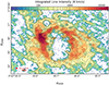 |
Fig. A.1. Same as Fig. 1 but for the CO(3-2) transition. The contours cover the same extent as the color bar with levels 3σ, 5σ, 10σ, 20σ, 40σ, 60σ, 100σ–400σ in steps of 50σ, where 1σ = 49.5 K km s−1. |
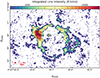 |
Fig. A.2. Same as Fig. 1 but for the CO(6-5) transition. The color ranges from 500 K km s−1 to the maximum value in logarithmic scale, and the contours have levels 3σ, 5σ, 10σ, 20σ, 40σ, 60σ, and 80σ, where 1σ = 99.9 K km s−1. |
Appendix B: Line ratio maps and LTE analysis results of regions based on high excitation
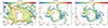 |
Fig. B.1. CO(3-2)/CO(2-1), CO(6-5)/CO(2-1), and CO(6-5)/CO(3-2) line ratio maps shown in the left, middle, and right panels, respectively. The color ranges from 0.1 to the maximum ratio for each plot. In the left panel, the contours span the same extent as the color bar with levels 0.1σ, 0.2σ, 0.4σ, 0.8σ, 1σ, 1.5σ, 2σ, 4σ, 6σ, 8σ, and 10σ where 1σ = 2.141273, the root-mean-square value from each ratio map. For the middle panel, the contour levels are 0.1σ, 0.2σ, 0.4σ, 0.8σ, 1σ, 1.5σ, 2σ, 3σ, 4σ, and 5σ with 1σ = 4.712347. The right panel contains contours with levels 0.05σ, 0.1σ, 0.2σ, 0.4σ, 0.6σ, 1σ, 1.5σ, 2σ, 3σ, 4σ, and 6σ, where 1σ = 5.144535. The symbols and markers for all panels are the same as in Fig. 1. |
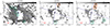 |
Fig. B.2. Region selection based on the AGN wind bicone, which is indicated by the purple lines, and excitation levels from the line ratio maps. The left, middle, and right panels are the region selections based on the CO(3-2)/CO(2-1), CO(6-5)/CO(2-1), and CO(6-5)/CO(3-2) ratio maps respectively. The number and color of each region correspond to those in the equivalent region code displayed in Table B.1. The dashed regions contain line ratios ≥3σ, while the solid regions only include line ratios ≥2σ. Other schematics of the region definitions are the same as Fig. 4. The underlying plots for all three panels are the corresponding line ratio maps from Fig. B.1. |
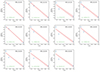 |
Fig. B.3. Rotational diagrams of regions defined based on line ratios. Region numbers are indicated at the upper right corner of each diagram. The rotational temperature values and their uncertainties are displayed in the lower-left corner of each diagram. All other symbols and markers of each rotational diagram are the same as inset plots in Fig. 5, except that the linear fit and its uncertainty are in red instead of purple. |
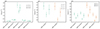 |
Fig. B.4. Total CO column densities (N) independently calculated from three CO transitions for all regions selected based on the CO(3-2)/CO(2-1) (left panel), CO(6-5)/CO(2-1) (middle panel), and CO(6-5)/CO(3-2) (right panel) line ratio. For each panel, the x-axis marks the region labels, while the y-axis indicates the total CO column densities in the unit of cm−2. The region code (along the x-axis) and color (the color of the data points) of each region match those in Table B.1. All other symbols and markers are the same as in Fig. 6. |
 |
Fig. B.5. Summary of rotational temperatures for all regions sampled around the CND defined based on the CO(3-2)/CO(2-1) (left panel), CO(6-5)/CO(2-1) (middle panel), and CO(6-5)/CO(3-2) (right panel) line ratio. For each panel, the x-axis marks the region labels, while the y-axis indicates the rotational temperatures in the unit of K. The region code (along the x-axis) and color (the color of the data points) of each region match those in Table B.1. All other symbols and markers are the same as in Fig. 7. |
Rotational temperatures and total CO column densities from 40×40 pc regions defined based on excitation.
Appendix C: Fitting results of line profiles for 40×40 pc regions defined based on the outflow
Fitting results of CO line profiles sampled from 40×40 pc regions defined based on outflow.
All Tables
Rotational temperatures and total CO column densities from CO gas in 40×40 pc regions defined based on outflow.
Optical depth values of CO gas in 40×40 pc regions defined based on the outflow.
Estimated lower and upper XCO factors for 40×40 pc regions defined based on the outflow.
Outflow speed away from the AGN position in the plane of the CND for 40×40 pc regions defined based on the outflow.
Rotational temperatures and total CO column densities from 40×40 pc regions defined based on excitation.
Fitting results of CO line profiles sampled from 40×40 pc regions defined based on outflow.
All Figures
|
Fig. 1. CO(2–1) velocity-integrated map in units of Kelvin kilometers per second (K km s−1) obtained with ALMA in the CND of NGC 1068. The color ranges from the minimum to the maximum value in the logarithmic scale, and the contour covers the same extent with levels 3σ, 5σ, 10σ, 20σ, 40σ, 60σ, 100σ–250σ in steps of 50σ, where 1σ = 50.6 K km s−1. Here, the 1σ value differs slightly from García-Burillo et al. (2019). We integrated over all channels instead of restricting to a certain range around vsys, which does not affect the velocity-integrated maps (this also applies to the CO(3–2) and CO(6–5) transitions, in comparison to García-Burillo et al. 2016). The smallest common beam size is indicated at the lower left corner of the figure, along with a linear scale indicator of 40 pc. The AGN position is also specified with two dashed lines. |
| In the text | |
|
Fig. 2. CO(2–1) velocity-width map of the CND in units of FWHM. The color scale spans the range [20, 200] km s−1, and the contours traverse the same range with a step size of 30 km s−1. The magenta lines trace the borders of the previously constructed AGN wind bicone (Das et al. 2006). The remaining markers and symbols are the same as in Fig. 1. |
| In the text | |
|
Fig. 3. CO(2–1) residual mean velocity field of the CND after the subtraction of projected CND rotation curve produced by García-Burillo et al. (2019). The color scale is within the range [−200, 200] km s−1 relative to the mean motion of the galaxy, vsys = 1120 km s−1, which is set to 0 km s−1. Blue (red) contours span from −200 (+50) to −50 (+200) km s−1 with a spacing of 25 km s−1 relative to vsys. The symbols and markers are the same as in Fig. 2. |
| In the text | |
|
Fig. 4. Region selection based on the AGN wind bicone indicated by the purple lines. The green regions are located either within the bicone or along the edge of the bicone, while the orange regions are outside the bicone. The numbers marked within each region match those in region codes displayed in Table 2 and are defined in Sect. 3.2. The background plot, including markers and symbols, is the de-colored CO(2–1) velocity-integrated map from Fig. 1. |
| In the text | |
|
Fig. 5. Rotational diagrams of all regions defined based on the outflow occupying the same locations on the background plot as assigned in the region definition in Sect. 3.2. Region numbers are listed in Table 2. The y-axis of the rotational diagrams is in the natural logarithmic scale (contrary to the “log10” scale used in some other literature), while the x-axis is in the linear scale, and their labels are showcased for region G6_40 (S). The blue data points with error bars within each plot are the weighted upper-level column densities from three CO transitions at their respective upper energy levels. The purple dashed line and the corresponding light purple shaded area are the fit based on the LTE condition and its uncertainty. The calculated rotational temperatures and their uncertainties are in green. The background plot is a cutout from Fig. 1, and the cutout region is indicated in brown in the inset plot at the upper-right corner. The AGN wind bicone was added as shaded solid purple lines in the background plot, and the sampled region size is indicated at the lower-left corner. All the other symbols and markers of the background plot are the same as Fig. 1. |
| In the text | |
|
Fig. 6. Total CO column densities (N) independently calculated from three CO transitions for all regions selected based on the outflow. The x-axis marks the region labels along with their locations around the CND (in brackets), while the y-axis indicates the total CO column densities in the unit of cm−2. The region code (along the x-axis) and color (the color of the data points) of each region match those in Table 2 and are defined in Sect. 3.2. The legend at the upper-right corner of the plot designates the symbols corresponding to the column densities calculated from three different CO transitions. |
| In the text | |
|
Fig. 7. Summary of rotational temperatures for all regions sampled around the CND defined based on the outflow in Sect. 3.2. The x-axis marks the region labels along with their locations around the CND (in brackets), while the y-axis indicates the rotational temperatures in the unit of K. The region code (along the x-axis) and color (the color of the data points) of each region match those in Table 2 and are defined in Sect. 3.2. The purple, yellow, pink, and lime dashed lines indicate the rotational temperatures at four different locations of the CND measured by Viti et al. (2014). |
| In the text | |
|
Fig. 8. CO(2–1) transition line profiles of all regions defined based on the outflow occupying the exact locations on the background plot as assigned in the region definition in Sect. 3.2. Region numbers, including their colors, are indicated at the upper-left corner of each plot. They correspond to those appearing in the region codes in Table 2 and are defined in Sect. 3.2. The x-axis of all line profile plots indicates the radial velocity of the gas, v, in the unit of km s−1. The y-axes are for the amount of emission within each channel, TB, in the unit of K. The blue data points and error bars within each region are the observed averaged line profile overplotted by the optimal fit as a green dashed line. The mean velocity of the galaxy, vsys, is indicated by the vertical red dash line for each line profile plot. Suppose the averaged line profile within one region was fit with a weighted multi-component Gaussian. All weighted Gaussian components are also provided in the plot as dotted lines using different colors (purple and orange for the first two components and brown for the third component). The transition of the line, CO(2–1), is indicated at the lower left corner of the background plot, and all other symbols are the same in the background plot as those in Fig. 5. |
| In the text | |
|
Fig. 9. CO(3–2) transition line profiles of all regions defined based on the outflow occupying the exact locations on the background plot as assigned in the region definition in Sect. 3.2. The background plot is the CO(3–2) velocity-integrated map from Fig. A.1. The transition of the line CO(3–2) is indicated at the lower left corner of the background plot. All other symbols and markers are the same as Fig. 8. |
| In the text | |
|
Fig. 10. CO(6–5) transition line profiles of all regions defined based on the outflow occupying the exact locations on the background plot as assigned in the region definition in Sect. 3.2. The background plot is the CO(6–5) velocity-integrated map from Fig. A.2. The transition of the line CO(6–5) is indicated at the lower left corner of the background plot. All other symbols and markers are the same as Fig. 8. |
| In the text | |
|
Fig. 11. Mean velocity values of all Gaussian components fit to the line profiles for the CO(2–1) (left panel), the CO(3–2) (mid panel), and the CO(6–5) (right panel) transitions on the scale of 40×40 pc. For each panel, the red shaded region marks ± one channel width away from the systematic velocity of the galaxy, vsys. Based on the weight parameter, round symbols correspond to the largest component of each fit, the diamond symbols correspond to the secondary component of each fit, and the square symbols correspond to the smallest component of each fit. The downward triangle symbol indicates the Gaussian component for absorption, and the “×” symbol implies large error bars. All other schematics are the same as Fig. 6. |
| In the text | |
|
Fig. 12. Velocity dispersion values of all Gaussian components fit to the line profiles for the CO(2–1) (left panel), the CO(3–2) (mid panel), and the CO(6–5) (right panel) transitions on the scale of 40×40 pc. All schematics follow that of Fig. 11. |
| In the text | |
|
Fig. 13. Scheme of the narrow-line region in NGC 1068 (not to scale). The ionized AGN wind (green) is blueshifted (blue arrows) on the front face and redshifted (red arrows) on the back, as viewed along the line of sight. Interaction between the AGN wind and the CND (yellow ellipses) drives molecular outflows, blueshifted in the south and redshifted in the north, as observed by ALMA. The tilt of the AGN wind relative to the CND affects outflow locations: in the north, it interacts farther from the AGN than the inner edge (marked by purple crosses) of the CND, while in the south, interaction occurs at the inner edge. As a result, the strongest molecular outflows emerge at the inner edge of the southern CND and farther from the inner edge in the northern CND. |
| In the text | |
|
Fig. 14. Projection of velocity (vgal) from NGC 1068 coordinates (primed) to sky coordinates (unprimed). The primed frame results from a i = 41° inclination rotation along the line of sight (from the negative z-axis to the z′-axis) and a PA = 289° rotation around z′-axis. The x′-axis aligns with the minor axis of the CND, matching the reference azimuthal direction (θ′0), with the 90° difference between x′ and y′-axes corresponding to the difference between PA and the θ′0 direction. The primed system follows a rightward primary axis convention, while the sky frame follows a northward reference. The PA reference axis is the x-axis after inclination rotation. The brown ball marks the molecular gas region, with outflow velocity vgal assumed to lie in the CND plane, directed radially from the AGN (red star). It decomposes as voutcos(θ) along x′-axis and voutsin(θ) along y′-axis, where θ is measured from x′-axis. Using Eq. (8), vgal is projected to sky velocity vsky, decomposed into the observed radial velocity vLOS and a transverse component (purple arrow), which further splits into vx and vy. |
| In the text | |
|
Fig. A.1. Same as Fig. 1 but for the CO(3-2) transition. The contours cover the same extent as the color bar with levels 3σ, 5σ, 10σ, 20σ, 40σ, 60σ, 100σ–400σ in steps of 50σ, where 1σ = 49.5 K km s−1. |
| In the text | |
|
Fig. A.2. Same as Fig. 1 but for the CO(6-5) transition. The color ranges from 500 K km s−1 to the maximum value in logarithmic scale, and the contours have levels 3σ, 5σ, 10σ, 20σ, 40σ, 60σ, and 80σ, where 1σ = 99.9 K km s−1. |
| In the text | |
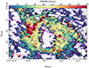 |
Fig. A.3. Same as Fig. 2 but for the CO(3-2) transition. |
| In the text | |
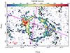 |
Fig. A.4. Same as Fig. 2 but for the CO(6-5) transition. |
| In the text | |
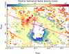 |
Fig. A.5. Same as Fig. 3 but for the CO(3-2) transition. |
| In the text | |
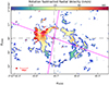 |
Fig. A.6. Same as Fig. 3 but for the CO(6-5) transition. |
| In the text | |
|
Fig. B.1. CO(3-2)/CO(2-1), CO(6-5)/CO(2-1), and CO(6-5)/CO(3-2) line ratio maps shown in the left, middle, and right panels, respectively. The color ranges from 0.1 to the maximum ratio for each plot. In the left panel, the contours span the same extent as the color bar with levels 0.1σ, 0.2σ, 0.4σ, 0.8σ, 1σ, 1.5σ, 2σ, 4σ, 6σ, 8σ, and 10σ where 1σ = 2.141273, the root-mean-square value from each ratio map. For the middle panel, the contour levels are 0.1σ, 0.2σ, 0.4σ, 0.8σ, 1σ, 1.5σ, 2σ, 3σ, 4σ, and 5σ with 1σ = 4.712347. The right panel contains contours with levels 0.05σ, 0.1σ, 0.2σ, 0.4σ, 0.6σ, 1σ, 1.5σ, 2σ, 3σ, 4σ, and 6σ, where 1σ = 5.144535. The symbols and markers for all panels are the same as in Fig. 1. |
| In the text | |
|
Fig. B.2. Region selection based on the AGN wind bicone, which is indicated by the purple lines, and excitation levels from the line ratio maps. The left, middle, and right panels are the region selections based on the CO(3-2)/CO(2-1), CO(6-5)/CO(2-1), and CO(6-5)/CO(3-2) ratio maps respectively. The number and color of each region correspond to those in the equivalent region code displayed in Table B.1. The dashed regions contain line ratios ≥3σ, while the solid regions only include line ratios ≥2σ. Other schematics of the region definitions are the same as Fig. 4. The underlying plots for all three panels are the corresponding line ratio maps from Fig. B.1. |
| In the text | |
|
Fig. B.3. Rotational diagrams of regions defined based on line ratios. Region numbers are indicated at the upper right corner of each diagram. The rotational temperature values and their uncertainties are displayed in the lower-left corner of each diagram. All other symbols and markers of each rotational diagram are the same as inset plots in Fig. 5, except that the linear fit and its uncertainty are in red instead of purple. |
| In the text | |
|
Fig. B.4. Total CO column densities (N) independently calculated from three CO transitions for all regions selected based on the CO(3-2)/CO(2-1) (left panel), CO(6-5)/CO(2-1) (middle panel), and CO(6-5)/CO(3-2) (right panel) line ratio. For each panel, the x-axis marks the region labels, while the y-axis indicates the total CO column densities in the unit of cm−2. The region code (along the x-axis) and color (the color of the data points) of each region match those in Table B.1. All other symbols and markers are the same as in Fig. 6. |
| In the text | |
|
Fig. B.5. Summary of rotational temperatures for all regions sampled around the CND defined based on the CO(3-2)/CO(2-1) (left panel), CO(6-5)/CO(2-1) (middle panel), and CO(6-5)/CO(3-2) (right panel) line ratio. For each panel, the x-axis marks the region labels, while the y-axis indicates the rotational temperatures in the unit of K. The region code (along the x-axis) and color (the color of the data points) of each region match those in Table B.1. All other symbols and markers are the same as in Fig. 7. |
| In the text | |
Current usage metrics show cumulative count of Article Views (full-text article views including HTML views, PDF and ePub downloads, according to the available data) and Abstracts Views on Vision4Press platform.
Data correspond to usage on the plateform after 2015. The current usage metrics is available 48-96 hours after online publication and is updated daily on week days.
Initial download of the metrics may take a while.