| Issue |
A&A
Volume 686, June 2024
|
|
|---|---|---|
| Article Number | A46 | |
| Number of page(s) | 23 | |
| Section | Extragalactic astronomy | |
| DOI | https://doi.org/10.1051/0004-6361/202449245 | |
| Published online | 28 May 2024 | |
AGN feedback in the Local Universe: Multiphase outflow of the Seyfert galaxy NGC 5506
1
Dipartimento di Fisica e Astronomia, Università degli Studi di Bologna, Via P. Gobetti 93/2, 40129 Bologna, Italy
e-mail: This email address is being protected from spambots. You need JavaScript enabled to view it.
2
Osservatorio di Astrofisica e Scienza dello Spazio (INAF–OAS), Via P. Gobetti 93/3, 40129 Bologna, Italy
3
Centro de Astrobiología (CAB), CSIC-INTA, Camino Bajo del Castillo s/n, 28692 Villanueva de la Cañada, Madrid, Spain
4
Observatorio de Madrid, OAN-IGN, Alfonso XII, 3, 28014 Madrid, Spain
5
INAF – Istituto di Radioastronomia, Via P. Gobetti 101, 40129 Bologna, Italy
6
Observatoire de Paris, LERMA, Collège de France, CNRS, PSL Université, Sorbonne Université, 75014 Paris, France
7
Max-Planck-Institut für Extraterrestrische Physik (MPE), Giessenbachstraße 1, 85748 Garching, Germany
8
Department of Physics, University of Oxford, Keble Road, Oxford OX1 3RH, UK
9
Instituto de Astrofísica de Canarias (IAC), Calle Vía Láctea, s/n, 38205 La Laguna, Tenerife, Spain
10
Departamento de Astrofísica, Universidad de La Laguna, 38206 La Laguna, Tenerife, Spain
11
Instituto de Física Fundamental, CSIC, Calle Serrano 123, 28006 Madrid, Spain
12
Departamento de Física de la Tierra y Astrofísica, Fac. de CC Físicas, Universidad Complutense de Madrid, 28040 Madrid, Spain
13
Instituto de Física de Partículas y del Cosmos IPARCOS, Fac. de CC Físicas, Universidad Complutense de Madrid, 28040 Madrid, Spain
14
Instituto de Radioastronomía and Astrofísica (IRyA-UNAM), 3-72 (Xangari), 8701 Morelia, Mexico
15
Department of Physics & Astronomy, University of Alaska Anchorage, Anchorage, AK 99508-4664, USA
16
Department of Physics & Astronomy, University of Southampton, Hampshire, SO17 1BJ Southampton, UK
17
Telespazio UK for the European Space Agency (ESA), ESAC, Camino Bajo del Castillo s/n, 28692 Villanueva de la Cañada, Spain
18
Space Telescope Science Institute, 3700 San Martin Drive, Baltimore, MD 21218, USA
19
Instituto de Estudios Astrofísicos, Facultad de Ingeniería y Ciencias, Universidad Diego Portales, Avenida Ejercito Libertador 441, Santiago, Chile
20
Kavli Institute for Astronomy and Astrophysics, Peking University, Beijing 100871, PR China
21
School of Mathematics, Statistics and Physics, Newcastle University, Newcastle upon Tyne NE1 7RU, UK
Received:
16
January
2024
Accepted:
22
February
2024
Abstract
We present new optical GTC/MEGARA seeing-limited (0.9″) integral-field observations of NGC 5506, together with ALMA observations of the CO(3 − 2) transition at a 0.2″ (∼25 pc) resolution. NGC 5506 is a luminous (bolometric luminosity of ∼1044 erg s−1) nearby (26 Mpc) Seyfert galaxy, part of the Galaxy Activity, Torus, and Outflow Survey (GATOS). We modelled the CO(3 − 2) kinematics with 3DBAROLO, revealing a rotating and outflowing cold gas ring within the central 1.2 kpc. We derived an integrated cold molecular gas mass outflow rate for the ring of ∼8 M⊙ yr−1. We fitted the optical emission lines with a maximum of two Gaussian components to separate rotation from non-circular motions. We detected high [OIII]λ5007 projected velocities (up to ∼1000 km s−1) at the active galactic nucleus (AGN) position, decreasing with radius to an average ∼330 km s−1 around ∼350 pc. We also modelled the [OIII] gas kinematics with a non-parametric method, estimating the ionisation parameter and electron density in every spaxel, from which we derived an ionised mass outflow rate of 0.076 M⊙ yr−1 within the central 1.2 kpc. Regions of high CO(3 − 2) velocity dispersion, extending to projected distances of ∼350 pc from the AGN, appear to be the result from the interaction of the AGN wind with molecular gas in the galaxy’s disc. Additionally, we find the ionised outflow to spatially correlate with radio and soft X-ray emission in the central kiloparsec. We conclude that the effects of AGN feedback in NGC 5506 manifest as a large-scale ionised wind interacting with the molecular disc, resulting in outflows extending to radial distances of 610 pc.
Key words: ISM: jets and outflows / ISM: kinematics and dynamics / galaxies: active / galaxies: clusters: individual: NGC 5506 / galaxies: Seyfert
© The Authors 2024
 Open Access article, published by EDP Sciences, under the terms of the Creative Commons Attribution License (https://creativecommons.org/licenses/by/4.0), which permits unrestricted use, distribution, and reproduction in any medium, provided the original work is properly cited.
This article is published in open access under the Subscribe to Open model. This email address is being protected from spambots. You need JavaScript enabled to view it. to support open access publication.
1. Introduction
The feedback from active galactic nuclei (AGN) has been proposed as a key mechanism influencing the course of galaxy evolution (see e.g. the reviews by Alexander & Hickox 2012; Fabian 2012; Kormendy & Ho 2013; Heckman & Best 2014; Harrison et al. 2018). AGN are powered by supermassive black holes (SMBHs) and their accretion discs located at galactic centres, emitting intense radiation and influencing the excitation and kinematics of the surrounding gas. This feedback process initiates from a very small region (10−3 pc is a typical accretion disc radius, see Cornachione et al. 2020; Guo et al. 2022; Jha et al. 2022), yet its effects can extend to influence the entire galaxy structure (Okamoto et al. 2005; Croton et al. 2006; Gaibler et al. 2012; McNamara & Nulsen 2012; Feruglio et al. 2015; Dubois et al. 2016; Anglés-Alcázar et al. 2017).
Analysing AGN feedback is a complex task due to its impact on different phases of the interstellar medium (ISM) across different physical scales, from the sub-parsec highly ionised ultra-fast outflows (UFOs, Tombesi et al. 2010; Fukumura et al. 2015; Nomura et al. 2016), warm absorbers (Blustin et al. 2005; Laha et al. 2014), and broad absorption lines (BALs, Weymann et al. 1991; Proga et al. 2000), to the kiloparsec-scale ionised (McCarthy et al. 1996; Baum & McCarthy 2000; Liu et al. 2013; Perna et al. 2020; Fluetsch et al. 2021) and molecular (Feruglio et al. 2010; Cicone et al. 2014; Bischetti et al. 2019; Ramos Almeida et al. 2022) outflows, up to the megaparsec-scale emission of giant radio galaxies (GRGs, Ishwara-Chandra & Saikia 1999; Kuźmicz et al. 2018; Dabhade et al. 2020) and X-ray groups and clusters (McCarthy et al. 2010; Fabian et al. 2011; McNamara & Nulsen 2012; Pasini et al. 2020).
Furthermore, AGN activity is considered to be intermittent over the course of a galaxy’s lifetime (King et al. 2004; Hopkins & Hernquist 2006; Schawinski et al. 2015; King & Nixon 2015), or even on timescales of days or less (Dultzin-Hacyan et al. 1992; Wagner & Witzel 1995). Consequently, comprehending the overall impact of AGN feedback is highly challenging, requiring the use of multiwavelength, multi-scale, and multi-time observations as essential tools.
The molecular phase of the ISM is of paramount importance, since it is the fuel for star formation and the phase in which the bulk of the gaseous mass in star-forming galaxies resides (e.g. Casasola et al. 2020). The AGN radiation heats the molecular gas by creating X-ray-dominated regions within the ISM (Maloney et al. 1996; Esposito et al. 2022, 2024; Wolfire et al. 2022), and it perturbs its kinematics, driving outflows (Cicone et al. 2014; Fiore et al. 2017; Veilleux et al. 2020; Lamperti et al. 2022).
Molecular gas typically forms a rotating disc associated with the galaxy gravitational potential. In AGN-host galaxies, a common form of perturbation involves the interaction between the molecular disc and the AGN hot wind, which manifests as outflowing ionised gas observable in X-rays (Cappi 2006; Tombesi et al. 2013; Giustini et al. 2023), UV (Hewett & Foltz 2003; Rankine et al. 2020) and optical (Fabian 2012; Mullaney et al. 2013) wavelengths (see also the review by Veilleux et al. 2020, and references therein, for the hot-cold gas coupling). In this regard, a multiwavelength approach is essential to effectively trace the multiphase outflow (Davies et al. 2014; Cicone et al. 2018; García-Bernete et al. 2021; Speranza et al. 2024). Nearby AGN serve as a perfect laboratory for studying these feedback signatures in detail, particularly with the increasingly improved spatial resolution and spectral coverage of today’s instruments.
The Galactic Activity, Torus, and Outflow Survey (GATOS) aims to understand the obscuring material (torus) and the nuclear gas cycle (inflows and outflows) in the immediate surroundings of the nuclear region of local AGN (García-Burillo et al. 2021; Alonso-Herrero et al. 2021; García-Bernete et al. 2024). The GATOS sample includes Seyfert galaxies with distances 10 − 40 Mpc, selected from the 70-month Burst Alert Telescope (BAT) catalogue of AGN (Baumgartner et al. 2013), some of which have been observed at different wavelengths, including optical and near-infrared integral field unit (IFU) spectroscopy, JWST, and ALMA observations.
One of the key findings of the GATOS survey is the existence of an anti-correlation between the nuclear molecular gas concentration and the AGN power: for a sample of 18 galaxies (García-Burillo et al. 2021) and an extended sample (García-Burillo et al., in prep.). Molecular gas, traced by low-J CO lines and observed by ALMA at a spatial resolution ∼10 pc, is also detected in outflows in those sources showing the most extreme nuclear-scale gas deficiencies, hence suggesting that the AGN power plays a role in clearing the nuclear region. These outflows have been observed and analysed in detail for some GATOS selected sources, which have been analysed in detail for the molecular and ionised phases (Alonso-Herrero et al. 2018, 2019, 2023; García-Bernete et al. 2021; Peralta de Arriba et al. 2023).
In this study, we investigate the molecular and ionised gas phases of NGC 5506, an Sa spiral galaxy in the GATOS sample at a redshift-independent distance of 26 Mpc (Karachentsev et al. 2006). At this distance the spatial scale is 125 pc/″. NGC 5506 has an AGN bolometric luminosity of ∼1.3 × 1044 erg s−1 (Davies et al. 2014) and is classified as an optically obscured narrow line Seyfert 1 (NLSy1, Nagar et al. 2002). The black hole mass is  (Gofford et al. 2015), yielding an Eddington ratio of
  . NGC 5506 is notable in the GATOS sample for having one of the highest molecular gas nuclear deficiencies (see Fig. 18 of García-Burillo et al. 2021), suggesting a potential imprint of AGN feedback on the molecular gas. Furthermore, NGC 5506 hosts a sub-parsec bent radio jet (Roy et al. 2000, 2001; Kinney et al. 2000) and a UFO (Gofford et al. 2013, 2015), making it an intriguing target for investigating multiphase (and multiscale) outflows. As a NLSy1, NGC 5506 is expected to be in a young AGN phase, characterised by a small black hole mass and a high accretion rate (see e.g. Crenshaw et al. 2003; Tarchi et al. 2011; Salomé et al. 2023). In Table 1 we report the fundamental parameters of NGC 5506.
Fundamental parameters for NGC 5506.
Evidence of complex kinematics from the long-slit optical spectrum was found by Wilson et al. (1985), who suggested radial motion for the ionised gas. Maiolino et al. (1994) refined this model, identifying outflowing velocities of up to 400 km s−1 for [OIII], [NII], and Hα, with the outflow cone inclined at −15° from the north. Additionally, Fischer et al. (2013) estimated an ionised outflow velocity of 500 km s−1 using slitless Hubble Space Telescope (HST) observations (see also Ruiz et al. 2005), modelling a biconical outflow. Davies et al. (2020) carried out a detailed analysis of optical data from observations made with X-shooter at VLT, finding a [OIII] outflow with a maximum velocity of 792 km s−1 and Ṁout = 0.21 M⊙ yr−1. Riffel et al. (2017, 2021) and Bianchin et al. (2022) studied the outflow of the ionised gas in the near-IR (with GEMINI NIFS), finding a mass outflow rate ranging from 0.11 to 12.49 M⊙ yr−1 (by adopting two fixed ne values – 500 cm−3 and 104 cm−3 – and exploring different geometries). The highest outflow values would result in a kinetic efficiency Ėout/Lbol = 0.71. They also calculate, from Lbol, a mass accretion rate to the SMBH of 0.067 M⊙ yr−1.
In this work, we present new IFU observations made with the Multi-Espectrógrafo en GTC de Alta Resolución para Astronomía (MEGARA) at the Gran Telescopio Canarias (GTC), which cover several optical emission lines, together with ALMA Band 7 observations of the CO(3 − 2) transition. The paper is structured as follows. In Sect. 2 we present the ALMA Band 7 and GTC/MEGARA observations. In Sect. 3 we describe the morphology of the molecular and ionised gas emission lines, while we model the kinematics of the two phases in Sects. 4 and 5, respectively. In Sect. 6 we discuss the results of this work and we compare our data with the available literature, and we draw our conclusions in Sect. 7.
2. Observations
2.1. ALMA Band 7
We observed NGC 5506 with the Band 7 ALMA receiver and a single pointing (project-ID: #2017.1.00082.S; PI: S. García-Burillo). We analysed the moderate resolution datacube from García-Burillo et al. (2021). The datacube has a 0.21″ × 0.13″ (26 pc × 16 pc) beam (with PA = − 60°, measured anticlockwise from the northern direction), a 17″ (2.1 kpc) field of view (FoV) and a largest angular scale of 4″ (0.5 kpc). To check the astrometry, we first aligned the HST/F606W image (top panel of Fig. 1) with the position of stars (from the Gaia mission), and then we aligned the ALMA continuum peak and the HST peak, resulting in α2000 = 14h13m14.877s, δ2000 = −03 ° 12′27.67″ (as in García-Burillo et al. 2021).
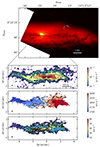 |
Fig. 1. Optical and molecular views of NGC 5506. Top: HST/F606W image of NGC 5506 from Malkan et al. (1998). The black rectangle identifies a region of 15.3″ × 5.1″ (corresponding to 1.9 × 0.6 kpc2). Bottom: ALMA CO(3 − 2) intensity, velocity and velocity dispersion maps, clipped at a signal-to-noise ratio of 3. The contours are between 10−3 and 10−1 Jy km s−1 (with 0.5 dex steps) for the intensity map, between 1700 and 2000 km s−1 (with 75 km s−1 steps) for the velocity map, and between 10 and 90 km s−1 (with 20 km s−1 steps) for the velocity dispersion map. North is up and east is left, and offsets in the ALMA maps are measured relative to the 870 μm continuum peak (as in García-Burillo et al. 2021), marked with a star symbol in every panel. The ALMA beam (0.21″ × 0.13″) appears in every bottom panel as a black ellipse in the lower left. |
2.2. GTC/MEGARA Bands B and R
We observed the central region of NGC 5506 on 20/03/2021 (Program GTC27-19B; PI: A. Alonso-Herrero), with MEGARA in IFU mode (Gil de Paz et al. 2016; Carrasco et al. 2018). We used two low resolution (LR) volume phase holographic gratings: the LR-B (spectral range ∼4300 − 5200 Å, resolution R ∼ 5000), to observe Hβ and the [OIII]λλ4959, 5007 doublet (exposure time 480 s), and the LR-R (∼6100 − 7300 Å, R ∼ 5900), to observe Hα, [OI]λ6300, and the [NII]λλ6548, 6583 and [SII]λλ6716, 6731 doublets (exposure time 400 s). The observed FoV is 12.5″ × 11.3″, corresponding to 1.6 × 1.4 kpc2.
The data reduction was performed by following Peralta de Arriba et al. (2023) and using the official MEGARA pipeline (Pascual et al. 2021). The resolution of the GTC/MEGARA observations was limited by the seeing conditions. We plotted it with a circle of diameter 0.9″ in all the relevant figures. The final datacubes were produced with a spaxel size of 0.3″, as recommended by the pipeline developers (Pascual et al. 2021; Peralta de Arriba et al. 2023): this corresponds to a physical spaxel size of 37.5 pc. We corrected the maps astrometry from the two configurations by aligning their continuum peaks with the ALMA Band 7 (870 μm) and HST (F606W filter) ones; to this point as the AGN position. We note that optical extinction may have an impact on the observed optical nucleus and actual AGN location on scales below the MEGARA seeing of 0.9″.
3. Morphology and kinematics
3.1. ALMA CO(3–2)
Fig. 1 shows the HST image and the ALMA CO(3 − 2) first three moments maps. The CO intensity map reveals an edge-on disc with a nuclear deficit (with respect to the circumnuclear region) of diameter ∼100 pc. This molecular gas depletion in the very centre has already been observed and analysed in García-Burillo et al. (2021). The circumnuclear disc is symmetric up to a diameter of ∼7″ = 875 pc. At radii larger than 3 − 4″ there is an extended gas tail in the eastern direction, which traces the dust lane visible in the HST image (see also Fig. 2).
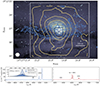 |
Fig. 2. Optical image and spectra of the central region of NGC 5506. Top panel: GTC/MEGARA [OIII] (λe = 5007 Å, in orange) and CO (λe = 870 μm, in blue) contours over the HST/F606W image of NGC 5506 (Malkan et al. 1998). The [OIII] contour levels, from the single-component Gaussian fit, have a logarithmic spacing from 3σ to 80% of the peak intensity in steps of 0.5 dex, while the CO(3 − 2) contours are the same of Fig. 1. The white star symbol is the AGN position, as determined in Sect. 2.2. The black and white squares are the nuclear region, with size 1.8 arcsec ∼225 pc, observed by X-shooter (see Davies et al. 2020), and the MEGARA FoV (12.5″ × 11.3″ ∼ 1.5 kpc × 1.4 kpc), respectively. The white circle in the bottom left is the MEGARA seeing conditions (diameter 0.9″). Bottom panel: left and right panels contain the spectra (integrated within the MEGARA FoV) revealed with the MEGARA LR-B and LR-R gratings, respectively, with names of identified emission lines and doublets. The inset is the zoom-in of a [OIII] line (after continuum subtraction): the blue shadings are the observed spectra of the MEGARA FoV and of the nuclear region, the black dashed lines are the fits with a single Gaussian. The inset axes have the same units of the outer panel. |
The bottom panels of Fig. 1 show the velocity and velocity dispersion of CO(3 − 2). The velocity field is centred at 1850 km s−1. It appears to be dominated by rotation, redshifted on the western side and blueshifted on the eastern side. However, it also exhibits perturbations due to non-circular motion. The velocity dispersion has a median value of 17 km s−1, and displays higher values along the NW–SE axis, with a maximum value of 86 km s−1 at δα ∼ 3″.
3.2. GTC/MEGARA emission lines
To derive the line intensity and kinematics, we extracted and fitted every spaxel of the MEGARA FoV with the ALUCINE1 (Ajuste de Líneas para Unidades de Campo Integral de Nebulosas en Emisión, Peralta de Arriba et al. 2023), initially with a single Gaussian and an amplitude-over-noise (AoN) of 3 or higher. Figure 2 shows the contours of the [OIII] doublet intensity, which are the brightest lines in the MEGARA spectrum (also in Fig. 2). The other identified emission lines, namely Hβ, [OI], Hα + [NII] doublet, and [SII] doublet, are labelled in Fig. 2.
The [OIII] emission of Fig. 2 nicely follows the HST image, and it is shaped as a bicone, typical of narrow line regions (NLRs; Pogge 1988; Wilson et al. 1993; Schmitt et al. 2003). The bicone emerges almost vertically in projection from the dusty molecular disc (∼20° anticlockwise from the north, as reported by Fischer et al. 2013; García-Burillo et al. 2021). We note here that Fischer et al. (2013) detected a one-sided ionisation cone (the northern side) using slitless spectroscopy of the [OIII] line. This is also evident in the HST map (Figs. 1 and 2). With MEGARA we detect the southern side as well, although it appears more extinguished. To check this we derived, following Cardelli et al. (1989), the visual extinction map from the Hα/Hβ line ratios (whereas the line fluxes come from the single Gaussian fit spaxel-by-spaxel). The resulting map (Fig. 3) shows a clear dust band crossing the southern side of NGC 5506 nuclear region. This piece of information also suggests that the southern side is the near side of the galaxy (in accordance with García-Burillo et al. 2021, analysis).
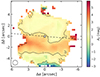 |
Fig. 3. Visual extinction map of the MEGARA FoV, calculated from the Hα/Hβ ratio and with RV = 3.1 (Cardelli et al. 1989). The white star symbol is the AGN position, and distances are relative to it. The dashed black line is our fiducial major kinematic axis with PA = 265° (see Sect. 4). The white circle in the bottom left is the MEGARA seeing conditions. |
It is tempting to interpret the comparison of [OIII] and CO contours in Fig. 2 as an ionised outflow that escapes the galaxy disc following the path of less resistance (Faucher-Giguère & Quataert 2012). We explore this possibility in Sect. 6.
4. Modelling the molecular gas kinematics
The CO(3 − 2) velocity field map (Fig. 1) shows the typical signatures of a rotating disc with some deviations from non-circular motions. We modelled the CO(3 − 2) datacube with 3DBAROLO2 (Di Teodoro & Fraternali 2015, hereafter 3DB), which creates a disc model for the rotating gas by dividing the emission into concentric rings, and fits the following parameters for every ring: the kinematic centre coordinates, the scale-height of the disc (z0), the inclination (i) of the disc with respect to the line of sight, the position angle (PA, measured anticlockwise from the northern direction for the receding side of the rotating disc) of the major kinematic axis, the systemic velocity vsys with which the whole galaxy is receding from us, the rotational velocity (vrot) of the gas, the velocity dispersion (σgas), and the radial velocity (vrad).
We note here that 3DB is designed to model the gas kinematics within a rotating disc (plus a radial velocity component). Our strategy is to use 3DB to identify and quantify any radial motion within the disc, which may point to an inflow or outflow of gas. If the radial flow forms an angle θout with the galaxy disc, only the velocity projected on the disc, that is, vout cos θout, will be detected by 3DB (see also Di Teodoro & Peek 2021; Bacchini et al. 2023).
We fixed the kinematic centre at the position of the continuum peak. We set a ring radial size of 0.15″ (≃19 pc), similar to the ALMA beam (0.21″ × 0.13″), and a total of 60 rings, thus reaching out to a distance of 9″ (≃1.1 kpc) from the centre.
4.1. Rotating disc
We performed a first 3DB run with vrad = 0 km s−1, and z0, i, PA, vsys, vrot, and σgas as free parameters. In this way we derived z0 = 0.2″ ≃ 25 pc, i = 80°, PA = 265°, and vsys = 1872 ± 10 km s−1 (where the error is given by the ALMA datacube spectral step). The inclination is the same as that found by García-Burillo et al. (2021) with the software kinemetry (Krajnović et al. 2006), while the PA is slightly different (they found PA = 275°). The vsys value is in agreement with several works: Fischer et al. (2013) reported 1823 km s−1, Riffel et al. (2017) 1878 km s−1, Davies et al. (2020) 1962 km s−1, García-Burillo et al. (2021) 1840 km s−1, and the average of these values is 1876 km s−1, only 4 km s−1 over our estimate.
We then performed a 3DB run with vrot and σgas as the only free parameters, while the others were fixed to the values determined in the first run. This approach assumes the absence of radial motions associated with molecular inflows or outflows. Figure 4 displays the position-velocity (PV) diagrams resulting from this run. Overall, the 3DB model contours (red lines in Fig. 4) reasonably reproduce the observed PV values (plotted with blue colours). From the major-axis PV diagram (Fig. 4, top panel) we can appreciate the goodness of the vsys estimate, as the CO(3 − 2) emission is symmetric with respect to vsys. Along the kinematic minor axis (Fig. 4, bottom panel), there are indications of non-circular motions in the central 1″, which we explore further in the next section.
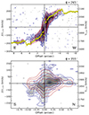 |
Fig. 4. ALMA CO(3 − 2) PV diagrams generated with 3DB along the kinematic major (top panel) and minor (bottom panel) axes. The grey scale and blue contours are the ALMA CO(3 − 2) observations > 3σ, while the red contours are the 3DB rotating disc model (without a radial velocity component). The yellow dots are the fitted rotation curve. The approximate eastern, western, southern, and northern directions are marked in the panels. |
4.2. Rotating disc with a radial velocity component
Within the approximate inner (projected) 1″, the minor axis PV diagram shows redshifted motions to the north of the AGN and blueshifted to the south (see top-left and bottom-right quadrants, respectively, of Fig. 4, bottom panel). Since the south is the near side of the galaxy (see Fig. 3 and related discussion in Sect. 3.2), this suggests the presence of a CO outflow component in the plane of the disc. We thus run another 3DB model including a radial velocity (vrad) component. The other free parameters are vrot and σgas, while the others have been set as the previous run.
Figure 5 shows the 3DB models and residuals for this run, for the first and second moments (mean velocity and mean velocity dispersion). The velocity and velocity dispersion absolute residuals have median values of 16 km s−1 and 14 km s−1, respectively. The highest velocity residuals (Fig. 5, second panel) are in the SE direction, where also the highest values of dispersion (Fig. 1, bottom panel) and dispersion residuals (Fig. 5, fourth panel) reside.
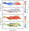 |
Fig. 5. Best-fit model and residuals (i.e. observation minus the model) obtained with 3DB for the rotating disc with a radial velocity component. Top and bottom panels show the mean velocity field and the velocity dispersion field of CO(3 − 2), respectively. In the first panel, vsys = 1872 km s−1 has been subtracted from the model velocities. Velocity contours (top panels) are at −50 and 50 km s−1 (solid) and at 0 km s−1 (dotted), while dispersion contours (bottom panels) are at −50, −25, 25, and 50 km s−1 (solid) and at 0 km s−1 (dotted). The dashed black line in the first panel is the kinematic major axis with PA = 265°. The ALMA beam appears in every panel as a black ellipse in the bottom left. |
Figure 6 shows the PV diagrams of this run, where we can appreciate a better fit along the minor axis (Fig. 6, bottom panel). Especially, the 3DB model now follows the northern red – southern blue asymmetry along the CO(3 − 2) minor axis. We also plot the mean velocities along the minor axis in Fig. 7, where we compare the 3DB results for the two models (with and without the radial velocity component). While not perfect, the model incorporating vrad more closely aligns with the observed data, particularly at positive offsets from the centre (i.e. in the northern direction). The yellow dots in the top panel represent the mean vrot (also plotted in the second panel of Fig. 8). We find vrot reaching 193 km s−1 at r = 3.5″ (440 pc), in reasonable agreement with the rotational velocity of 181 ± 5 km s−1 measured from HI absorption (Gallimore et al. 1999).
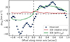 |
Fig. 7. Relative velocities of CO(3 − 2) along the minor axis, extracted and averaged from a slit width of 3 pixels (corresponding to a projected width of 0.09″). The blue circles are the observed values, not weighted for the emitted flux. The green and red lines are the 3DB models with and without a radial velocity component. |
The four panels in Fig. 8 show, from top to bottom, the CO(3 − 2) surface density ΣCO(3 − 2), and the modelled rotational velocity vrot, velocity dispersion σgas, and radial velocity  (which is the same as vrad, with the positive sign meaning outflowing and negative meaning inflowing gas). We distinguish significative changes in the curve profiles at two particular radii: 0.4″ and 5″.
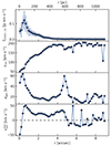 |
Fig. 8. Radial profiles of the molecular gas derived with 3DB. From top to bottom: the CO(3 − 2) surface density, the rotational velocity (same as the yellow dots in the top panel of Fig. 6), the velocity dispersion and the outflow velocity, all as a function of deprojected distance from the AGN (on the plane of the galaxy). The dashed black line in the bottom panel is the zero line, dividing between ouflow ( |


At r ∼ 0.4″ (50 pc) we find the maximum value of ΣCO(3 − 2), which corresponds to the inner radius of the ring. Within this radius  , which is indicative of inflowing gas: it could be an indication of AGN feeding from the molecular disc (see e.g. Combes 2021), but since we only have two radial points we could not confirm this finding. At r ∼ 0.4″ we also have a peak in the σgas and
  profiles: this means that the molecular ring is not only rotating, but also outflowing (as in NGC 1068, see García-Burillo et al. 2019).
At r ∼ 5″ (610 pc) there is another peak of σgas, and  goes from positive to negative, suggesting a transition from outflow to inflow (García-Burillo et al. 2014, found a similar result for NGC 1068). However, at r > 5″ there is a lot of oscillation between inflow and outflow, probably due to the small number of datapoints (see the asymmetry of the CO emission in Fig. 1), so we did not take into consideration these outer radii.
The CO(3 − 2) radial motion on the molecular plane could be explained with (i) inflowing/outflowing gas (García-Bernete et al. 2021; Ramos Almeida et al. 2022) or (ii) elliptical orbits associated with a bar (Buta & Combes 1996; Casasola et al. 2011; Audibert et al. 2019). Since the presence of a bar is not evident on the CO(3 − 2) PV diagrams (Figs. 4 and 6, cf. Alonso-Herrero et al. 2023), it probably does not dominate the motion of the molecular gas. Nevertheless, due to this possibility, we conservatively assume that the outflow velocities we derive between  (50 pc) and
  (610 pc) are upper limits. We discuss the presence of a bar in NGC 5506 in Sect. 6.1.
4.3. The molecular mass outflow rate
We used the CO(3 − 2) emission between  (50 pc) and
  (610 pc) to calculate the main properties of the outflow, such as the amount of molecular gas it is driving outwards (
 ). To do so, we first converted it to CO(1 − 0), using a typical brightness temperatures ratio for galaxy discs of r31 ≡ TB, CO(3 − 2)/TB, CO(1 − 0) = 0.7: this is the average value found by Israel (2020) in 126 nearby galaxy centres, and we adopt it for consistency with García-Burillo et al. (2021). We then used a Galactic CO-to-H2 conversion factor of XCO = 2 × 10²⁰ mol cm−2 (K km s−1)−1 (Bolatto et al. 2013). We chose the Galactic value to better compare our results with most of the literature, and also because NGC 5506 does not show any indication of merger and is not particularly luminous in the infrared (LIR = 1010.49 L⊙, Sanders et al. 2003). We calculate
  between
  and
and  . This result depends on our choice of r31 and XCO. Specifically, a higher brightness temperatures ratio r31 ∼ 1, as found in the central ∼1″ of NGC 1068 (García-Burillo et al. 2014; Viti et al. 2014), would decrease
  . Conversely, a lower r31 ∼ 0.4 (i.e. within 1σ of the values collected by Israel 2020), would increase
  . Also a lower XCO ∼ 0.8 × 10²⁰ mol cm−2 (K km s−1)−1, usually associated to starburst galaxies (Bolatto et al. 2013; Pérez-Torres et al. 2021), would decrease
  . The combined uncertainty of these two conversions could decrease the calculated mass by a multiplicative factor of ≈0.28 or increase it by a factor of ≈1.75.
Assuming a simple shell geometry (as in Alonso-Herrero et al. 2023), we can write the mass outflow rate as
 (1)
(1)
where  is defined as the average velocity measured between
  and
and  . By taking the standard deviation as its uncertainty, we find
  km s−1, from which we infer a molecular mass outflow rate of
  yr−1 (which includes the helium contribution).
Figure 9 shows the radial profile of the mass outflow rate, i.e. the same calculation of Eq. (1) for every radial ring. To account for different r31 and XCO, we plotted errorbars in Fig. 9 corresponding to the typical ranges r31 = 0.4 − 1 and XCO = (0.8 − 2)×1020 mol cm−2 (K km s−1)−1. We find a strong peak of  at the inner radius of the molecular ring (R ∼ 85 pc), which is outflowing (while rotating) up to
  yr−1. A second (minor) peak is visible around 250 pc (∼2″), within which resides half of the molecular mass, and which corresponds to a small vout peak (bottom panel of Fig. 8).
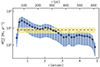 |
Fig. 9. Molecular gas mass outflow rate as a function of the deprojected distance from the AGN (on the plane of the galaxy). The molecular gas mass includes the helium contribution. The blue dots correspond to the values computed with the 3DB model radial velocities and CO(3 − 2) intensities of Fig. 8. The blue shading and errorbars represent the variation in r31 and XCO (see text for details). The red dashed line is the integrated mass outflow rate, 8 ± 3 M⊙ yr−1, with the shaded yellow region representing its uncertainty. |
The average value of  yr−1 is similar to those of other local Seyfert, which range from ∼1 M⊙ yr−1 to a few tens of M⊙ yr−1 (Combes et al. 2013; García-Burillo et al. 2014; Morganti et al. 2015; Alonso-Herrero et al. 2019, 2023; Domínguez-Fernández et al. 2020; García-Bernete et al. 2021).
5. Modelling the ionised gas kinematics
5.1. Gaussian decomposition
In the inset of Fig. 2 we presented the single Gaussian fit of the [OIII] line. It is evident that a single Gaussian cannot accurately reproduce the complex shape of the line profile. Consequently, we decided to fit the observed lines (listed in Fig. 2) with two Gaussians, spaxel by spaxel. The ALUCINE code determines, based on the AoN > 3 cut, whether one or two Gaussians are necessary for each spaxel. As input parameters, ALUCINE needs also the wavelength range for subtracting the continuum, and a systemic velocity. At first we set vsys, CO = 1872 km s−1 as the CO(3 − 2), but we achieved better results by setting vsys, [OIII] = 1893 km s−1. It is worth noting that this 21 km s−1 difference is only 1.5 times the MEGARA spectral step (∼14 km s−1). A detailed comparison of vsys values from the literature is available in Davies et al. (2020) and in Sect. 4.1.
We name the two Gaussians “narrow” and “broad” component, where their width is the discriminant factor. We focus mainly on the [OIII] line in the analysis, since it shows the highest signal (Fig. 2) and is the one usually studied for AGN ionised winds (Weedman 1970; Heckman et al. 1981; Veilleux 1991; Crenshaw & Kraemer 2000; Harrison et al. 2014). The results for the [OIII] line are in Fig. 10. The top panels show the narrow component: from the velocity map we can identify a rotation pattern, with velocities up to −100 and 100 km s−1, oriented roughly in the same way of the CO disc (Fig. 1). The external parts of the narrow component can be hardly associated to rotation however: at the northern end of the FoV the gas reaches 340 km s−1 (with relatively low dispersions around 60 km s−1), while at NE and NW there are areas with very high dispersion (up to ∼200 km s−1). It could be that these extreme northern regions trace the external part of the ionised outflow.
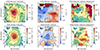 |
Fig. 10. [OIII] double Gaussian fit made with ALUCINE. Top and bottom rows are for the narrow and broad component, respectively. From left to right, the three columns show the intensity, velocity, and velocity dispersion of both components. The AGN position is marked with a black star symbol, and distances are measured from it. The white circle in the bottom left of each panel is the MEGARA seeing conditions. The velocity panels (central column) show the PA = 265° and 355° dashed black lines, and two black rectangles that highlight the northern and southern edges of the velocity field. |
The broad component of [OIII] (bottom panels of Fig. 10) contains fewer pixels than the narrow one, since for some spaxels a single Gaussian component was sufficient to obtain a proper modelling (or the broad Gaussian had AoN < 3). The velocity map of this component displays a central blueshifted region (up to −170 km s−1), and some positive and negative velocities all over the FoV. The velocity dispersion map reaches higher values than the narrow one (up to 400 km s−1).
The Gaussian decomposition made with ALUCINE is able to separate the [OIII] rotation from the outflow component (except for the extreme northern regions at high velocity or velocity dispersion). The same applies for the other emission lines in the MEGARA spectrum, for which the results are shown in Appendix B. Compared to [OIII], the narrow component intensity maps of [NII], [SII], and [OI] are more consistent with an ionised rotating disc (aligned with the HST and ALMA discs, i.e. with PA ∼ 265°), while the broad component is more elongated on the north-south direction, (as [OIII], Hα and Hβ). This north-south elongation is especially evident in the velocity dispersion of the broad components of [NII] and [SII] (Figs. B.3 and B.4).
We also show, in Appendix C, the Baldwin, Phillips, Telervich (BPT) diagrams (Baldwin et al. 1981; Veilleux & Osterbrock 1987; Kewley et al. 2001; Kauffmann et al. 2003) made with the same fitted lines. From such diagrams (Figs. C.1–C.3) we can conclude that most of the observed central emission is due to the AGN activity rather than star formation, both for the narrow and broad components.
We explain how we used this decomposition to calculate the [OIII] mass of the broad component in Sect. 5.3. However, the velocities obtained with ALUCINE represent mean velocities within each spaxel. To explore the full range of velocities of the ionised gas, we produced [OIII] PV diagrams (Fig. 11), along the same PAs as the CO emission (Fig. 6). In both major- and minor-axis PV diagrams, the ionised gas exhibits velocities exceeding 1000 km s−1, both redshifted and blueshifted. The most extreme blueshifted velocities (Δvlos < −1500 km s−1) are possibly contaminated with emission from the secondary [OIII] doublet line (λe = 4959 Å). The major-axis PV diagram (Fig. 11, top panel) displays a rotation curve between −100 and 100 km s−1. However, most of the emission, along both PAs, appears to be dominated by the outflowing gas. Along the minor axis (bottom panel of Fig. 11), there is also an observable X shape, elongated at large radii, likely due to the northern red and southern blue regions in the central panels of Fig. 10 (within the black rectangles). These regions may represent the locations where the outflow is emerging from the nuclear zone.
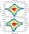 |
Fig. 11. PV diagrams of the observed [OIII] (λe = 5007 Å) line, clipped at 3σ, along major (top panel) and minor (bottom panel) kinematic axes, with PA = 265° and 355°, respectively. Contours are at [10, 30, 100, 300, 1000]σ. The vertical dashed line is the AGN position, and the horizontal dashed line is the systemic velocity |

To have a better understanding of the observed PV diagrams, we show, in Fig. 12, the [OIII] line profile at three locations along the minor axis. The northern (in red) and southern (in blue) regions exhibit two distinct components: one travelling at approximately the systemic velocity, and the other outflowing at ∼ ± 300 km s−1. The southern blue emission also displays a stronger centred emission, which is evident in the PV diagram (Fig. 11, bottom panel) at ≳4″ south (while its northern counterpart is fainter). In the Gaussian decomposition (Fig. 10), the northern region with high redshifted velocities likely belongs to the outflowing and broad component rather than to the rotational/narrow one. However, the associated flux (and consequently, the ionised mass within it) is negligible in our analysis (see Sect. 5.3).
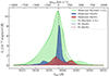 |
Fig. 12. Observed spectra (continuum-subtracted) of the [OIII]λ5007 line at three locations along the kinematical minor axis (PA = 355°). In green, blue, and red shadings, the spectra extracted within the nuclear region (black square in Fig. 2), the southern region, and the northern region (black rectangles in Fig. 10), respectively. With the same colours, the lines are the ALUCINE two-component fits for the same regions. Note that for the nuclear and southern regions a third component would be needed to fit the residual blueshifted and redshifted components, respectively. The nuclear spectrum is multiplied by a 0.2 factor for a better comparison. The vertical dashed line is the redshifted (with |

We note here that, even if several works allow three or more Gaussians to fit the emission of [OIII] in AGN with possible outflows (e.g Harrison et al. 2014; Dall’Agnol de Oliveira et al. 2021; Speranza et al. 2022; Hermosa Muñoz et al. 2024), we limited our analysis to two components to have a simpler interpretation of them: we associated the narrow component to the ionised gas rotation, and the broad one to the outflow. Adding more Gaussians to the ALUCINE fit would result in higher velocities and velocity dispersions for the broader components (but we refer to the next section for a better characterisation of the outflow velocities). However, such broader components would add a small contribution to the modelled flux (see Fig. A.1), hence to the outflow mass.
5.2. Non-parametric [OIII] velocities
In the previous section we saw that the ionised gas (traced by [OIII]) shows very high velocities probably due to an AGN wind. However, due to the complex line profiles, it is hard to see the different velocities from the Gaussian decomposition of Fig. 10. In this section, we make use of a non-parametric method to measure the outflow velocities.
We followed the method described by Harrison et al. (2014) to spatially resolve the velocities of the [OIII] emission line. This method uses the [OIII] line produced as the sum of the two fitted Gaussians (Sect. 5.1). For every spaxel we calculate the velocities corresponding to different percentiles to the flux contained in the modelled line profile, namely the velocities at the 2nd, 5th, 10th, 90th, 95th, and 98th percentiles, respectively called v02, v05, v10, v90, v95, and v98. We also calculate, for every spaxel, the velocity of the emission line peak vp.
The results are illustrated in Fig. 13. The top-left panel shows vp, which is similar to the velocity of the narrow component of the Gaussian decomposition (cf. Fig. 10). It has been shown that vp traces the ionised gas rotation (Rupke & Veilleux 2013; Harrison et al. 2014). In the case of NGC 5506, vp is similar to the mean-velocity field of the molecular gas, whose kinematic PA = 265° is plotted with a dashed black line. The region ∼5″ N from the AGN, redshifted at ∼300 km s−1, is not following the rotation pattern.
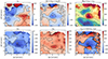 |
Fig. 13. Non-parametric velocity components for the [OIII] line. The top panels show, from left to right, the peak velocity vp, the broad velocity Δv, and the 80% width W80. The bottom panels show, from left to right, the velocity at the 2nd flux percentile (v02), at the 98th (v98), and the positive or negative velocities that have the maximum absolute value between these two (for every spaxel), which is our estimate for the outflow velocity vout. The white star symbol marks the AGN position, and the dashed black line in the top-left panel is the kinematic major axis (PA = 265°). The white circle in the bottom left of each panel is the MEGARA seeing conditions. Velocities in all the panels are in km s−1. |
The top-central panel of Fig. 13 shows the Δv = (v05 + v95)/2 map. This is very similar to the velocity map of the broad component modelled by ALUCINE (cf. Fig. 10), and so represents its velocity offset. There are differences between the two maps though, especially around ∼3″ NE from the nucleus, where the Δv plot shows redshifted velocities around 50 km s−1. This may be an outflow feature lost in the ALUCINE decomposition map.
The top-right panel of Fig. 13 is the W80 = v90 − v10 width, which represents the width containing 80 percent of the [OIII] emitted flux. In the case of a single modelled Gaussian, this would correspond approximately to the FWHM. In our decomposition, W80 is, in a way, a combination of the velocity dispersions of the two components of Fig. 10. However, W80 exhibits larger values across the entire FoV, particularly at the AGN position (reaching up to 500 km s−1) and in the ∼5″ N region (with an average < W80, N > ∼500 km s−1). The maximum value observed is W80, max = 826 km s−1 located ∼6″ W.
The bottom three panels of Fig. 13 show the velocities found in the 2nd and 98th percentiles of the flux (the third panel is showing the positive or negative velocities that have the maximum absolute value among the two). These correspond to the projected maximum values for the outflow velocities (as in Rupke & Veilleux 2013; Harrison et al. 2014; Davies et al. 2020). We find the highest blueshifted velocities around the AGN (−565 km s−1 at the AGN position, −620 km s−1 at ∼1″ S-SW) and in the ∼5″ N region (up to −702 km s−1). The highest redshifted values are found at ∼1.6″ (200 pc) S–SW from the AGN (up to 551 km s−1), and very close to the ∼5″ N region (up to 689 km s−1).
The prevalence of blueshifted velocities in the nuclear region was previously identified in the X-shooter spectrum, extracted with a FoV of 1.8 × 1.8 arcsec2 (Davies et al. 2020), which is also visible in Fig. 12 (green profile). With the MEGARA data, we observe high-velocity components, not associated with rotation, both blueshifted and redshifted, in all panels of Fig. 13 and in nearly every direction, particularly in the central 4 × 4 arcsec2, as evident in Fig. 11. This may be due to a wide bicone aperture, where any given line of sight intersects both approaching and receding clouds of gas simultaneously.
We isolate the [OIII] rotation velocity (vrot) by taking the median absolute value of vp along the PA = 265° line (the dashed line in the vp panel of Fig. 13) with a width of 4 pixels (corresponding to 1.2″ ∼ 150 pc). In Fig. 14, we plot the mean radial profiles of vrot, Δv, W80, and vout. The [OIII] rotational velocity vrot flattens out at 83 km s−1 around ∼320 pc from the centre (Fig. 14, top panel), whereas the CO(3 − 2) flattens out at 193 km s−1 around r = 440 pc (Fig. 8, top panel). We point out that [OIII] is not the best tracer for the ionised disc rotation, and in fact it is the slowest rotator among the MEGARA lines: Hα flattens at 120 km s−1, Hβ at 113 km s−1, [NII] at 120 km s−1, [SII] at 118 km s−1, and [OI] at 110 km s−1 (see Appendix D for the mean velocity radial profiles of all the MEGARA lines).
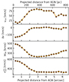 |
Fig. 14. Radial profiles for the different mean velocities of the [OIII] line, all as a function of the projected distance from the AGN. Panels show, from top to bottom: the rotational velocity vrot along the kinematic axis, the broad velocity Δv, the 80% width W80, and our estimate for the mean outflow velocity of the ionised gas |

Interestingly, the ionised gas seems to be rotating at 60% the velocity of the molecular gas. Davis et al. (2013) found that, in CO-rich ATLAS3D galaxies (Cappellari et al. 2011), the difference between molecular and ionised rotation velocities was larger for [OIII]-bright galaxies (up to a Δvrot ∼ 80 km s−1), due to the different ionisation sources: a bright [OIII] emission (with respect to Hβ) traces a dynamically hotter component of ionised gas than HII regions embedded in the cold star-forming disc. Also Levy et al. (2018) and Su et al. (2022) found the ionised gas to rotate slower than the molecular gas in EDGE-CALIFA (Bolatto et al. 2017) and ALMaQUEST (Lin et al. 2019) galaxies, but with a smaller difference of ∼25 km s−1.
The radial profiles of Δv, W80, and vout have similar shapes, with a smooth decrease of absolute velocities from the centre up to a radial distance of ∼400 pc. For these three quantities, the distance is the projected distance along every direction, so one has to be careful when comparing them to vrot or to the molecular radial profiles of Figs. 8 and 9. We used the vout radial profile of Fig. 14 to calculate the other ionised outflow properties, as the mass outflow rate (see Sect. 5.4).
5.3. The [OIII] outflow mass
In this section we calculate the electron density and mass of the ionised outflow. To do so, we make use of the ALUCINE decomposition (Sect. 5.1), and we consider the flux of the broad component as the outflow (whereas the narrow component is associated to the ordered gas rotation). We subsequently explain how we calculated the outflow properties using the [OIII] emission line (Fig. 10), but we also exploited the modelled broad components of Hα, Hβ, and [NII] (Figs. B.1–B.3).
One of the challenges in the estimation of the ionised outflow mass is to properly calculate the gas volume density n, usually expressed as the electron density ne (where for ionised gas we expect ne ∼ n). Many studies assume constant fiducial values for ne (e.g. Harrison et al. 2014; Fiore et al. 2017) for all the spaxels (or for a whole sample of galaxies). The most commonly used method to estimate ne pixel-by-pixel is based on the [SII] doublet ratio (Osterbrock & Ferland 2006). However, this method has known biases, one of which is that the doublet ratio saturates above 104 cm−3. We refer the interested reader to Davies et al. (2020) for a structured discussion on this topic and for a comparison between different methods to estimate ne.
We follow Baron & Netzer (2019), Davies et al. (2020), and Peralta de Arriba et al. (2023), in estimating the ionised gas density from the ionisation parameter log U, defined as the number of ionising photons per atom, U = QH/(4πr2nHc), where QH is the rate of hydrogen-ionising photons (in s−1 units), r is the distance from the ionising source, nH ∼ ne is the hydrogen density, and c is the speed of light. Since QH can be estimated from the AGN bolometric luminosity (Baron & Netzer 2019), we can find ne given the ionisation parameter.
Since the [OIII]/Hβ and [NII]/Hα line ratios are widely used in AGN studies (Veilleux & Osterbrock 1987; Kewley et al. 2001), and both depend on log U, Baron & Netzer (2019), by exploiting a sample of 234 type II AGN with outflow signatures, empirically determined (with a scatter of 0.1 dex) the following expression:
![Mathematical equation: $$ \begin{aligned} \log U &= -3.766 + 0.191 \log \left( \frac{[\mathrm{OIII}]}{\mathrm{H}\beta } \right) + 0.778 \log ^2 \left( \frac{[\mathrm{OIII}]}{\mathrm{H}\beta } \right)\nonumber \\& \quad - 0.251 \log \left( \frac{[\mathrm{NII}]}{\mathrm{H}\alpha } \right) + 0.342 \log ^2 \left( \frac{[\mathrm{NII}]}{\mathrm{H}\alpha } \right). \end{aligned} $$](/articles/aa/full_html/2024/06/aa49245-24/aa49245-24-eq34.gif) (2)
(2)
The resulting log U map for the broad component of [OIII] is in the left panel of Fig. 15. There are fewer pixels than the broad [OIII] map (Fig. 10, bottom panels), since we had to use also the broad Hα, Hβ, and [NII] maps, and only the pixels featured in all four maps are left (with Hβ being the most limiting one). We recover a median value of log U = −2.9, in agreement with the integrated value of −2.87 ± 0.12 found by Davies et al. (2020) within the X-shooter FoV (1.8 × 1.8 arcsec2).
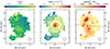 |
Fig. 15. From left to right: outflowing [OIII] ionisation parameter log U, electron density ne, and mass |

From the log U definition, we follow Baron & Netzer (2019) and calculate the electron density as
 (3)
(3)
where we used the log(Lbol/ erg s−1) = 44.1 ± 0.09 obtained by Davies et al. (2020) from the X-ray luminosity given by Ricci et al. (2017). For the central pixel we set r equal to half the pixel size.
We show the spatially resolved ne map in the central panel of Fig. 15. We find ne to decrease at increasing distance from the centre, as found by other works on local AGN (e.g. Freitas et al. 2018; Shimizu et al. 2019; Davies et al. 2020; Peralta de Arriba et al. 2023). The maximum ne, max = 8.5 × 105 cm−3 is exactly at the AGN position. To compare our values with the results of Davies et al. (2020) for NGC 5506, we calculate the median ne at the edge of a 1.8 × 1.8 arcsec2 FoV (the black square in Fig. 2), finding log(ne/cm−3) = 3.95, which is very close to their integrated value of log(ne/cm−3) = 4.03 ± 0.14.
Before calculating the ionised outflow mass from the broad [OIII] luminosity, we have to correct it for the extinction. To do so, we assume an intrinsic ratio Hα/Hβ = 3.1, and we use the Cardelli et al. (1989) extinction law (RV = 3.1). We find the [OIII] outflow area (i.e. the same of the three panels in Fig. 15) to have a median AV = 1.9 mag and an extinction-corrected total luminosity Lbroad[OIII] = 1041.6 erg s−1. If we limit the FoV to 1.8 × 1.8 arcsec2 we find 1041.3 erg s−1, in excellent agreement with the Davies et al. (2020) value of 1041.2 erg s−1.
Finally, the ionised outflow mass  is given by (see Rose et al. 2018; Baron & Netzer 2019):
![Mathematical equation: $$ \begin{aligned} M_{\rm out}^\mathrm{ion} = \frac{\mu m_{\rm H} L_{\mathrm{broad [OIII]}}}{\gamma _{\mathrm{[OIII]}} n_e}, \end{aligned} $$](/articles/aa/full_html/2024/06/aa49245-24/aa49245-24-eq38.gif) (4)
(4)
where μ = 1.4 is the mean molecular weight, mH is the hydrogen mass, Lbroad[OIII] is the extinction-corrected broad [OIII] luminosity, ne is the outflowing gas electron density, and γ[OIII] is the effective line emissivity, which depends on the ionisation parameter (see Eqs. (5) and (6) in Baron & Netzer 2019). We interpolated the values listed in Baron & Netzer (2019), Table 2, to calculate γ[OIII] for every spaxel.
The resulting spatial distribution of the outflowing [OIII] mass is presented in the right panel of Fig. 15. We calculated a total ionised outflowing mass of  . In comparison, the mass reported by Davies et al. (2020) is 3.2 × 10⁴ M⊙. The discrepancy arises because the MEGARA aperture is significantly larger than the X-shooter one (as indicated by the white and black squares in Fig. 2). Additionally, Davies et al. (2020) used a single value for all the quantities involved in Eq. (4), whereas we considered spatial variations, resulting in a more dispersed distribution of
  .
.
5.4. The ionised mass outflow rate
We calculate the ionised mass outflow rate following, as for the molecular gas, Eq. (1) (as in Rose et al. 2018; Baron & Netzer 2019; Davies et al. 2020). The outflow velocity and mass have been calculated following Sects. 5.2 and 5.3. If we take, as typical outflow radius,  pc (i.e. the one that contains 95% of Mout), we find
  km s−1, from which we infer a ionised mass outflow rate of
  yr−1, where the uncertainty comes from the standard deviation of the different measured radial velocities.
This is significantly lower than the 0.21 M⊙ yr−1 value reported in Davies et al. (2020). A factor of ∼2 discrepancy is due to the different velocity (they measured 792 km s−1). Another difference is the outflow size, that dilutes the averaged value (their aperture radius was of 117 pc). We can recover the Davies et al. (2020) value if we plot the radial profile of Ṁout (Fig. 16) using, for each radius, the maximum outflow velocity available (dashed black line) rather than the average one (solid black line).
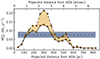 |
Fig. 16. Radial profile of the ionised mass outflow rate |


The spatially resolved map of ionised mass outflow rate (Fig. 17) reveals an excess of  , extending from ∼0.8″ up to ∼2.5″ south of the AGN. This is the region where the most extreme blueshifted velocities of 620 km s−1 reside (see Fig. 13). It is also a region which exhibit some excess of Mout (see Fig. 15, right panel), hence the local high Ṁout. Some minor Ṁout clumps are visible at ∼1.5″ NW and ∼2.5″ NE from the AGN. Interestingly, this NE clump (which is very clear in the Mout map) is located just after the separation between blueshifted and redshifted velocities (on the red side) in the bottom-left panel of Fig. 13. All together these clumps contribute to the two main bumps in the Ṁout radial profile (Fig. 16).
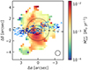 |
Fig. 17. Coloured map of the ionised mass outflow rate, with contours of observed CO(3 − 2) velocity dispersion (as Fig. 1, bottom panel), at 30 and 50 km s−1 in light and dark blue, respectively. The two black circles have a radius of 100 and 250 pc (i.e. ∼0.8 and 2 arcsec, respectively) from the white star symbol, which marks the AGN position. The dashed line is the kinematic major axis. The white circle in the bottom right is the MEGARA seeing conditions. |
The farthest (from the AGN) peak, at ∼4″ ∼ 500 pc north, visible in both Figs. 16 and 17, is due to the pixels in the northern region highlighted in the central panels of Fig. 10, and whose spectrum is plotted in red in Fig. 12. Most of this northern region has been excluded from our analysis since it is out of the log U map (Fig. 15, left panel) and therefore of all the subsequent maps (this is mainly due to the limited size of the broad component of the Hβ line, see Fig. B.2), but probably it is part of the ionised outflow. Interestingly, some molecular clouds are visible just north of the MEGARA FoV edge in Fig. 2.
Another region left out by Fig. 15 is the NW arc with high W80 values (Fig. 13), associated with LINER/shock emission in Figs. C.2 and C.3. This arc begins at the western edge of the CO(3 − 2) emission, but it may be linked to the high dispersion values we see going towards NW (bottom panel of Figs. 1 and 17). These two regions may indicate that the outflow (both in the ionised and molecular phases) has a larger size than the ones we derive with the present analysis. However, a more detailed mapping of the aforementioned areas is needed to draw meaningful conclusions.
The immediate vicinity of the AGN is relatively devoid of  , due to the small amount of
  (see Fig. 15) in this region. This may stem from the observed ionised wind being a past outflow episode, now situated ∼100 pc from the centre, where it encounters resistance from the surrounding ISM. This corresponds to the same distance at which we observe a peak in the molecular mass outflow rate (Fig. 9), with the caveat that we are seeing projected distances for the ionised outflow, and deprojected distances (on the disc plane) for the molecular outflow. We subsequently compare the two phases in detail in the next section.
6. Discussion
6.1. The case for elliptical motions due to a bar
Being highly inclined, it is challenging to prove (or disprove) the presence of a bar in NGC 5506. de Vaucouleurs et al. (1991) classified this galaxy as a peculiar edge-on Sa, while Baillard et al. (2011), by analysing SDSS images, signalled the presence of a “barely visible” stellar bar (with confidence ranging from “no bar” to “bar long about half D25”). By inspecting PanSTARRS images we could in fact recognise an X-shape, typical of edge-on barred galaxies (Baba et al. 2022).
Edge-on barred galaxies typically display clearly separate components on the gas PV diagrams (see e.g. the compilation by Bureau & Freeman 1999). This is not evident on the molecular PV diagrams of NGC 5506 (Figs. 4 and 6), whereas instead it is noticeable on the major axis of NGC 7172 (Alonso-Herrero et al. 2023, Figs. 8 and 10), which is also a highly inclined galaxy. With the exception of the X-shape on the minor axis (explained in Sect. 5.1, see also Fig. 12), the same applies for the PV diagrams of the ionised gas (Fig. 11). This, however, could be to an unfavourable orientation of the bar, being too close to the minor axis to produce any apparent perturbation. It is also worth noting that NLSy1s as NGC 5506 are usually associated with the presence of a bar (Crenshaw et al. 2003).
The fact that we see disturbed molecular clouds on the north-west and south-east (Fig. 1, bottom panel), may be an indication of interaction of the ionised outflow with the molecular disc (Fig. 17). In the following section, we aim to provide a more comprehensive description of the interaction. However, it is important to note that we cannot rule out the potential existence of a bar within the central kiloparsec. Consequently, in our analysis of molecular inflow/outflow velocities (Fig. 8, bottom panel), we treat these results as upper limits.
6.2. Comparing molecular and ionised outflows
In Sect. 4 we modelled the ALMA CO(3 − 2) kinematics, finding a rotating disc along PA = 265°, within which the gas is also outflowing. The most intense region of the molecular outflow is at r ∼ 100 pc, with  km s−1 and
  yr−1. This is also where most of the molecular mass resides. Another region of interest is at r ∼ 250 pc, where we found a second, more modest, peak of
  yr−1. We plotted the circles of radii 100 and 250 pc in Fig. 17. If we follow the PA = 265° dashed line on the eastern side, we find enhanced values of
  at such radii. This could be an evidence of interaction between the ionised AGN wind and the molecular disc, where we are seeing perhaps two different outflow episodes, in which case, from the 150 pc distance between the episodes, we can calculate, given a 500 km s−1 velocity, a Δtout = 0.3 Myr (similar to the AGN flickering timescale derived by Schawinski et al. 2015; King & Nixon 2015).
We can have a closer look at the interaction between the ionised and molecular gas by plotting the CO(3 − 2) dispersion contours against the ionised mass outflow rate map, as in Fig. 17: not only do the  regions at 100 and 250 pc east from the AGN correlate with high CO dispersion (σCO ≥ 50 km s−1), but also the region ∼1.5″ NW has both a local excess of
  and high σCO (up to 61 km s−1). From Fig. 17 (but also from Fig. 1) it seems NGC 5506 would be in the weak coupling scenario described by Ramos Almeida et al. (2022), i.e. where the biconical ionised outflow intercepts the molecular disc only partially, launching a modest molecular outflow (see also Alonso-Herrero et al. 2023). This would be in agreement with the bicone model fitted by Fischer et al. (2013) for NGC 5506: they found the inclination between the bicone and the host galaxy disc to be 32°, less than the maximum half-opening angle of the bicone (40°, see Table 6 in Fischer et al. 2013).
We draw a tentative sketch of the relative positions of the molecular disc and the ionised bicone in Fig. 18. Every line of sight intercepts both approaching and receding sides of the bicone, resulting in a mix of blueshifted and redshifted velocities (as in Fig. 13). Once we are far enough from the disc plane (∼5″ north and south), the edges of the bicone start to appear distinct on the spectra (Fig. 12): this would point out a hollow bicone. The southern nearest and northern farthest bicone edges intercept the molecular disc, hence rising the CO velocity dispersion and causing the molecular ring to outflow on the disc plane: this results in high CO dispersion on the SE–NW direction (Fig. 17), and in an asymmetry in the CO(3 − 2) PV diagram on the redshifted northern – blueshifted southern directions (Fig. 6, bottom panel).
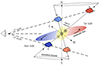 |
Fig. 18. Scenario (not to scale) for the intersection between the molecular disc (the red and blue ellipse) and the ionisation bicone. In the disc of the galaxy, traced by the molecular gas, we mark the AGN position (white star) and the proposed interactions between the two gas phases (black asterisk symbols). The 300-pc radio (at 8.46 GHz) and soft X-ray (below 1 keV) emission is depicted in yellow. Along the ±5″ lines of sight, we draw clouds on the edge of the bicone, colour-coded depending on whether the gas is blueshifted or redshifted. |
An exception to the spatial correlation between σCO and  is in the immediate vicinity of the AGN: there the CO line broadening is probably due to the presence, in a small space, of multiple components of CO velocities, even due to ordered rotation alone. Nevertheless, this region also has a deficit of CO emission (see Fig. 1 and García-Burillo et al. 2021), which may be another indication of multiphase feedback.
If we adopt the scenario drawn in Fig. 18, then the ionised outflow velocities we measured, especially the redshifted ones in the north and the blueshifted in the south, are lower limits due to projection effects. We did not perform a modelling of the bicone (so its opening angle in Fig. 18 is only qualitative), but if we adopt an half-opening angle of 40° (Fischer et al. 2013), we can derive a multiplicative factor of 1/sin(40 ° ) = 1.56, which would result in an average deprojected  km s−1. Being the deprojected
  affected in the same way, this would not change the
  .
.
If the AGN wind seen with the [OIII] and the outflowing CO ring are physically connected, we expect the kinetic energy rate (Ėout) or the momentum rate (Ṗout) to be conserved (see King & Pounds 2015, and references therein). These two quantities can be straightforwardly calculated as  and Ṗout = Ṁoutvout. The values (listed in Table 2) point to a energy-driven rather than momentum-driven outflow (King & Pounds 2015; Veilleux et al. 2020): in such outflows, the momentum undergoes a boost (e.g. Veilleux et al. 2020; Longinotti et al. 2023), which in our case is Ṗmol/Ṗion = 7. However, if we use the values derived by Davies et al. (2020) for the ionised outflow, the ratio of the momentum rates would be ∼1.2, rather indicating a momentum-driven outflow. Given the observed Lbol and λEdd (see Table 1), a radiation pressure-driven wind would predict an outflow of ∼3 M⊙ yr−1 (Hönig 2019), not too far from our
  value: this also would point to a momentum-driven scenario.
Results for the molecular and ionised phases of the AGN outflow.
We highlight that the dichotomy between energy and momentum conservation refers to single or continuous outflow episodes. In the case of NGC 5506, we may be observing the stratification of multiple outflows, a possibility explored also in the next section. Taking everything into account, if the ionised wind is pushing and dragging the molecular gas, it currently seems to impact only the inner part of the molecular ring. At this stage, the AGN wind appears to be relatively ineffective in clearing the entire galaxy (which is common in local systems, see e.g. Fluetsch et al. 2019).
6.3. Extending the spectrum: radio and X-ray literature
Despite its classification as a radio-quiet galaxy (Terao et al. 2016), NGC 5506 has been detected in the radio band in several studies. Wehrle & Morris (1987) detected, with the VLA at 5 GHz, a radio bubble, NW from the nucleus, also visible in the 8.46 GHz VLA A-array continuum image presented by Schmitt et al. (2001). In Fig. 19 we plot the contours of Schmitt et al. (2001) VLA image against the ionised mass outflow rate map, where we can see that the radio bubble observed by Wehrle & Morris (1987) perfectly overlaps with the ∼1.5″ region that has both high  and high σCO. The extended ∼300 pc VLA emission in Fig. 19 is well aligned with the galactic disc (PA = 265°), but extends below and (mostly) over it, following the [OIII] emission. Orienti & Prieto (2010) measured, for this diffuse radio emission, a steep spectral index α = 0.9, which combined with the size < 1 kpc, would make it a compact steep spectrum (CSS) radio source (e.g. Dallacasa et al. 2013; O’Dea & Saikia 2021).
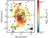 |
Fig. 19. Same as Fig. 17 but with the Schmitt et al. (2001) 3.6 cm VLA contours, at log(Sν/Jy beam−1) = (−4, −3.5, −3, −2.5, −2), in black. The black circle in the bottom right is the MEGARA seeing conditions, with the VLA beam ellipse within it in white. |
The VLA contours shown in Fig. 19 are also spatially coincident with the soft X-ray (below 1 keV) emission observed, with the Chandra X-ray Observatory, by Bianchi et al. (2003). Their main explanation is that the photoionised gas (that we clearly see with MEGARA, Fig. 2, even if more extended than 300 pc) is reprocessing the nuclear X-ray emission. However, since we detect velocities up to ∼600 km s−1 out to 300 pc from the AGN, the expected temperature of the shocked emission is kT ≈ 1.3(vshock/103)2 keV ≈ 0.5 keV (Fornasini et al. 2022), which could suggest a thermal emission for the Chandra soft X-ray observation (see also Paggi et al. 2012).
High-resolution radio observations made with the Very Long Basement Array (VLBA) at different frequencies (1.6–15 GHz, Roy et al. 2000), show a sub-relativistic (vjet ≤ 0.25c) one-sided jet, initially oriented 70° anticlockwise from the north (so roughly as the CO disc), and then bending 90° towards the south (Kinney et al. 2000), at 3.4 pc (∼0.03″) from the core emission. In Roy et al. (2001) they argue that the counterjet is not visible because of free-free absorption (rather than doppler boosting), and that the bend might be a sign of interaction between the jet and the NLR gas on parsec scales. Middelberg et al. (2004) collected different-epochs EVN, MERLIN and VLBA observations, and reported a 3σ upper limit of 0.50c for the jet motion with respect to the core. Gallimore et al. (2006) argue that the diffuse emission on the 300-pc scale (Fig. 19 and Schmitt et al. 2001), is attributed to the parsec-scale jet observed by Roy et al. (2000). The misalignment between the jet trajectory (initially pointing at ∼70° anticlockwise from north and later bending ∼90° towards the south) and the elongation of the diffuse radio emission towards the north direction can be explained by either jet precession or jet-ISM interactions (Gallimore et al. 2006, and also Xanthopoulos et al. 2010 come to the same conclusions).
Interestingly, such high velocities are also seen via absorption of the hard X-ray Fe XXVI Lyα line. The UFO in NGC 5506 has been observed and studied by Gofford et al. (2013, 2015), where they find vUFO = 0.246 ± 0.006 c. The momentum rate released by such a UFO ranges between 5 × 1033 and 5 × 1035 dyn, where this large uncertainty mostly comes from the estimation of the distance between the UFO and the AGN (see Tombesi et al. 2013, for a detailed derivation of the UFO parameters). Even the lower limit of  is 3.8 times the molecular one (see Fig. 20). If we accept as good all these different measurements, a plausible explanation for this momentum decrease (instead of the boost required in the energy-driven scenario, or the constant Ṗout in the momentum-driven scenario) is, again, that we are seeing different outflow episodes, among which the UFO is the most recent (also Sebastian et al. 2020, suggest multiple activity episodes for NGC 5506 from analysing polarised radio data). X-ray observations have shown in fact continuous rapid variation among different epochs (McHardy & Czerny 1987; Uttley & McHardy 2005; Sun et al. 2018), even suggesting the presence of a supermassive black hole binary system (Manchanda 2006).
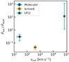 |
Fig. 20. Outflow momentum rate divided by the AGN radiation momentum rate Lbol/c (also called wind momentum load) as a function of the outflow velocity vout for the molecular gas (in blue), the ionised gas (in orange), and the UFO (in green). |
Both relativistic jets (e.g. Mukherjee et al. 2018; Audibert et al. 2023, but also low-power jets, e.g. Venturi et al. 2021; Pereira-Santaella et al. 2022) and UFOs (e.g. Marasco et al. 2020; Longinotti et al. 2023; Salomé et al. 2023) are thought to be the initial trigger of galaxy-scale ionised and molecular outflows (see Singha et al. 2023, for a recent discussion). Another possibility is that the VLBI radio structures seen by Roy et al. (2000) are shock signatures left by the X-ray UFO (Longinotti et al. 2018).
7. Summary and conclusions
We presented new GTC/MEGARA optical IFU observations of NGC 5506, complemented with ALMA Band 7 observations of the CO(3 − 2) transition (García-Burillo et al. 2021). NGC 5506 is a nearby (D = 26 Mpc) luminous (Lbol ∼ 1.3 × 1044 erg s−1) Seyfert galaxy, part of the GATOS sample (García-Burillo et al. 2021; Alonso-Herrero et al. 2021). The angular resolution of the ALMA observation (0.21″ × 0.13″) allows us to probe regions on physical scales of ∼25 pc for the molecular gas. The GTC/MEGARA observation, with a seeing of 0.9″ (corresponding to ∼113 pc at the distance of NGC 5506), offers a spectral resolution enabling the analysis of velocities as low as ∼14 km s−1.
The CO(3 − 2) map reveals a highly inclined (i = 80°) cold molecular gas ring, symmetric up to a radius of 3.5″ ∼ 438 pc, with an eastern tail extending up to a 8″ ∼ 1 kpc radius. The cold molecular gas mass of the ring is ∼2.3 × 10⁸ M⊙, calculated assuming a brightness temperature ratio of TB, CO(3 − 2)/TB, CO(1 − 0) = 0.7 and a Galactic CO-to-H2 conversion factor. The CO(3 − 2) kinematics reveal a rotating disc, flattening at 193 km s−1 around r = 440 pc, with clear signatures of non-circular motions. A 3DBAROLO model of a rotating disc with a radial velocity component reproduces reasonably well the observed CO kinematics, interpreted as a rotating and outflowing molecular ring. Within a 0.4″ radius, fitted radial velocities are directed towards the centre, potentially indicating AGN feeding, though this finding could not be confirmed since this radius is very close to the ALMA beam size. At larger radii, the radial velocity is directed outwards, decreasing from a maximum of 50 km s−1 to an average of 26 km s−1. The maximum molecular outflow radius is 610 pc, within which we calculate an integrated molecular gas mass outflow rate of ∼8 ± 3 M⊙ yr−1.
We detected several bright emission lines in the MEGARA spectra, with [OIII]λ5007 standing out as the brightest. The spatially resolved BPT diagnostic diagrams predominantly reveal Sy-like excitation, ruling out a significant contribution from star formation over a projected region of 1.5 kpc × 1.4 kpc. The [OIII] kinematics appear to be dominated by the outflowing gas. Nevertheless, we separated disc rotation from non-circular motion spaxel-by-spaxel, employing both parametric and non-parametric methods. The ionised gas exhibits a slower rotation speed than the molecular gas (∼190 km s−1), with Hα, [NII] and [SII] reaching 120 km s−1. Conversely, we detected [OIII] radial velocities up to 1000 km s−1, both approaching and receding. Emplying a non-parametric analysis of the line wings of [OIII] emission, we derived an average ionised gas outflow velocity of 422 km s−1 within a radius of 525 pc. To estimate the outflowing mass, we utilised the broad component intensity maps from the double Gaussian decomposition. We calculated the electron density in every spaxel using the ionisation parameter method. This analysis yielded an outflowing mass of 9.8 × 10⁴ M⊙, resulting in an ionised mass outflow rate of  yr−1.
yr−1.
We compared the spatially resolved map of  with the CO(3 − 2) velocity dispersion map, identifying spatial correlation between the two. The ionised outflow does not appear perpendicular to the plane of the galaxy; instead, it likely lies at a small angle relative to the disc. This results in a good geometrical coupling between the two phases. We also found diffuse radio and soft X-ray emission to spatially correlate with the observed [OIII] emission and
  .
.
Various results, both from this study and the literature, suggest a diverse history of outflows for NGC 5506. These outflows may be associated with the presence of a parsec-scale radio jet, a 0.25c UFO, or a combination of both. New ALMA and JWST observations, offering a higher resolution view of the nuclear region of NGC 5506, will soon become available as part of the GATOS project. These observations may eventually enhance our understanding of the complex interactions between the sub-parsec radio jet, the UFO, the ionised wind, and the molecular torus and disc.
Available at https://gitlab.com/lperalta_ast/alucine
Available at https://bbarolo.readthedocs.io
Acknowledgments
We thank the anonymous referee for suggestions and comments that helped to improve the presentation of this work. We acknowledge the use of Python (Van Rossum & Drake 2009) and the following libraries: Astropy (Astropy Collaboration 2013, 2018), CMasher (van der Velden 2020), Matplotlib (Hunter 2007), NumPy (Harris et al. 2020), Pandas (Pandas development team 2020), pvextractor (Ginsburg et al. 2016), Seaborn (Waskom 2021), SciPy (Virtanen et al. 2020), and SpectralCube (Ginsburg et al. 2019). This research is based on observations made with the NASA/ESA Hubble Space Telescope obtained from the Space Telescope Science Institute, which is operated by the Association of Universities for Research in Astronomy, Inc., under NASA contract NAS 5–26555. These observations are associated with program 5479. This paper makes use of the following ALMA data: ADS/JAO.ALMA#2017.1.00082.S. ALMA is a partnership of ESO (representing its member states), NSF (USA) and NINS (Japan), together with NRC (Canada), MOST and ASIAA (Taiwan), and KASI (Republic of Korea), in cooperation with the Republic of Chile. The Joint ALMA Observatory is operated by ESO, AUI/NRAO and NAOJ. This research has made use of “Aladin sky atlas” developed at CDS, Strasbourg Observatory, France (Bonnarel et al. 2000). This research has made use of the NASA/IPAC Extragalactic Database (NED), which is funded by the National Aeronautics and Space Administration and operated by the California Institute of Technology. The authors acknowledge the use of computational resources from the parallel computing cluster of the Open Physics Hub (https://site.unibo.it/openphysicshub/en) at the Physics and Astronomy Department in Bologna. F.E. acknowledges support from grant PRIN MIUR 2017-20173ML3WW_s, and funding from the INAF Mini Grant 2022 program “Face-to-Face with the Local Universe: ISM’s Empowerment (LOCAL)”. A.A.H. and L.H.M. acknowledge support from research grant PID2021-124665NB-I00 funded by MCIN/AEI/10.13039/501100011033 and by ERDF “A way of making Europe”. S.G.B. acknowledges support from the Spanish grant PID2022-138560NB-I00, funded by MCIN/AEI/10.13039/501100011033/FEDER, EU. I.G.B. acknowledges support from STFC through grant ST/S000488/1 and ST/W000903/1. L.P.d.A. acknowledges financial support from grant PGC2018-094671-B-I00 funded by MCIN/AEI/10.13039/501100011033 and by ERDF “A way of making Europe”. M.P.S. acknowledges funding support from the Ramón y Cajal program of the Spanish Ministerio de Ciencia e Innovación (RYC2021-033094-I). C.R.A. acknowledges support from EU H2020-MSCA-ITN-2019 Project 860744 “BiD4BESt: Big Data applications for black hole Evolution STudies”, from project “Feeding and feedback in active galaxies”, with reference PID2019-106027GB-C42, funded by MICINN-AEI/10.13039/501100011033, and from project “Tracking active galactic nuclei feedback from parsec to kiloparsec scales”, with reference PID2022-141105NB-I00. E.B. acknowledges the María Zambrano program of the Spanish Ministerio de Universidades funded by the Next Generation European Union and is also partly supported by grant RTI2018-096188-B-I00 funded by the Spanish Ministry of Science and Innovation/State Agency of Research MCIN/AEI/10.13039/501100011033. O.G.M. acknowledges finantial support from UNAM through the project PAPIIT IN109123 and from CONAHCyT through the project “Ciencia de Frontera 2023” CF-2023-G-100. C.R. acknowledges support from Fondecyt Regular grant 1230345 and ANID BASAL project FB210003.
References
- Alexander, D. M., & Hickox, R. C. 2012, New Astron. Rev., 56, 93 [Google Scholar]
- Alonso-Herrero, A., Pereira-Santaella, M., García-Burillo, S., et al. 2018, ApJ, 859, 144 [Google Scholar]
- Alonso-Herrero, A., García-Burillo, S., Pereira-Santaella, M., et al. 2019, A&A, 628, A65 [NASA ADS] [CrossRef] [EDP Sciences] [Google Scholar]
- Alonso-Herrero, A., García-Burillo, S., Hönig, S. F., et al. 2021, A&A, 652, A99 [NASA ADS] [CrossRef] [EDP Sciences] [Google Scholar]
- Alonso-Herrero, A., García-Burillo, S., Pereira-Santaella, M., et al. 2023, A&A, 675, A88 [NASA ADS] [CrossRef] [EDP Sciences] [Google Scholar]
- Anglés-Alcázar, D., Faucher-Giguère, C.-A., Quataert, E., et al. 2017, MNRAS, 472, L109 [Google Scholar]
- Astropy Collaboration (Robitaille, T. P., et al.) 2013, A&A, 558, A33 [NASA ADS] [CrossRef] [EDP Sciences] [Google Scholar]
- Astropy Collaboration (Price-Whelan, A. M., et al.) 2018, AJ, 156, 123 [Google Scholar]
- Audibert, A., Combes, F., García-Burillo, S., et al. 2019, A&A, 632, A33 [NASA ADS] [CrossRef] [EDP Sciences] [Google Scholar]
- Audibert, A., Ramos Almeida, C., García-Burillo, S., et al. 2023, A&A, 671, L12 [NASA ADS] [CrossRef] [EDP Sciences] [Google Scholar]
- Baba, J., Kawata, D., & Schönrich, R. 2022, MNRAS, 513, 2850 [NASA ADS] [CrossRef] [Google Scholar]
- Bacchini, C., Mingozzi, M., Poggianti, B. M., et al. 2023, ApJ, 950, 24 [NASA ADS] [CrossRef] [Google Scholar]
- Baillard, A., Bertin, E., de Lapparent, V., et al. 2011, A&A, 532, A74 [NASA ADS] [CrossRef] [EDP Sciences] [Google Scholar]
- Baldwin, J. A., Phillips, M. M., & Terlevich, R. 1981, PASP, 93, 5 [Google Scholar]
- Baron, D., & Netzer, H. 2019, MNRAS, 486, 4290 [Google Scholar]
- Baum, S. A., & McCarthy, P. J. 2000, AJ, 119, 2634 [NASA ADS] [CrossRef] [Google Scholar]
- Baumgartner, W. H., Tueller, J., Markwardt, C. B., et al. 2013, ApJS, 207, 19 [Google Scholar]
- Bianchi, S., Balestra, I., Matt, G., Guainazzi, M., & Perola, G. C. 2003, A&A, 402, 141 [NASA ADS] [CrossRef] [EDP Sciences] [Google Scholar]
- Bianchin, M., Riffel, R. A., Storchi-Bergmann, T., et al. 2022, MNRAS, 510, 639 [Google Scholar]
- Bischetti, M., Piconcelli, E., Feruglio, C., et al. 2019, A&A, 628, A118 [NASA ADS] [CrossRef] [EDP Sciences] [Google Scholar]
- Blustin, A. J., Page, M. J., Fuerst, S. V., Branduardi-Raymont, G., & Ashton, C. E. 2005, A&A, 431, 111 [CrossRef] [EDP Sciences] [Google Scholar]
- Bolatto, A. D., Wolfire, M., & Leroy, A. K. 2013, ARA&A, 51, 207 [CrossRef] [Google Scholar]
- Bolatto, A. D., Wong, T., Utomo, D., et al. 2017, ApJ, 846, 159 [Google Scholar]
- Bonnarel, F., Fernique, P., Bienaymé, O., et al. 2000, A&AS, 143, 33 [NASA ADS] [CrossRef] [EDP Sciences] [Google Scholar]
- Bureau, M., & Freeman, K. C. 1999, AJ, 118, 126 [NASA ADS] [CrossRef] [Google Scholar]
- Buta, R., & Combes, F. 1996, Fund. Cosmic Phys., 17, 95 [Google Scholar]
- Cappellari, M., Emsellem, E., Krajnović, D., et al. 2011, MNRAS, 413, 813 [Google Scholar]
- Cappi, M. 2006, Astron. Nachr., 327, 1012 [NASA ADS] [CrossRef] [Google Scholar]
- Cardelli, J. A., Clayton, G. C., & Mathis, J. S. 1989, ApJ, 345, 245 [Google Scholar]
- Carrasco, E., Gil de Paz, A., Gallego, J., et al. 2018, in Ground-based and Airborne Instrumentation for Astronomy VII, eds. C. J. Evans, L. Simard, H. Takami, et al., SPIE Conf. Ser., 10702, 1070216 [NASA ADS] [Google Scholar]
- Casasola, V., Hunt, L. K., Combes, F., García-Burillo, S., & Neri, R. 2011, A&A, 527, A92 [NASA ADS] [CrossRef] [EDP Sciences] [Google Scholar]
- Casasola, V., Bianchi, S., De Vis, P., et al. 2020, A&A, 633, A100 [NASA ADS] [CrossRef] [EDP Sciences] [Google Scholar]
- Cicone, C., Maiolino, R., Sturm, E., et al. 2014, A&A, 562, A21 [NASA ADS] [CrossRef] [EDP Sciences] [Google Scholar]
- Cicone, C., Brusa, M., Ramos Almeida, C., et al. 2018, Nat. Astron., 2, 176 [Google Scholar]
- Combes, F. 2021, in Galaxy Evolution and Feedback across Different Environments, eds. T. Storchi Bergmann, W. Forman, R. Overzier, & R. Riffel, 359, 312 [NASA ADS] [Google Scholar]
- Combes, F., García-Burillo, S., Casasola, V., et al. 2013, A&A, 558, A124 [NASA ADS] [CrossRef] [EDP Sciences] [Google Scholar]
- Cornachione, M. A., Morgan, C. W., Millon, M., et al. 2020, ApJ, 895, 125 [Google Scholar]
- Crenshaw, D. M., & Kraemer, S. B. 2000, ApJ, 532, L101 [Google Scholar]
- Crenshaw, D. M., Kraemer, S. B., & Gabel, J. R. 2003, AJ, 126, 1690 [NASA ADS] [CrossRef] [Google Scholar]
- Croton, D. J., Springel, V., White, S. D. M., et al. 2006, MNRAS, 365, 11 [Google Scholar]
- Dabhade, P., Röttgering, H. J. A., Bagchi, J., et al. 2020, A&A, 635, A5 [NASA ADS] [CrossRef] [EDP Sciences] [Google Scholar]
- Dallacasa, D., Orienti, M., Fanti, C., Fanti, R., & Stanghellini, C. 2013, MNRAS, 433, 147 [CrossRef] [Google Scholar]
- Dall’Agnol de Oliveira, B., Storchi-Bergmann, T., Kraemer, S. B., et al. 2021, MNRAS, 504, 3890 [CrossRef] [Google Scholar]
- Davis, T. A., Alatalo, K., Bureau, M., et al. 2013, MNRAS, 429, 534 [Google Scholar]
- Davies, R. I., Maciejewski, W., Hicks, E. K. S., et al. 2014, ApJ, 792, 101 [Google Scholar]
- Davies, R., Baron, D., Shimizu, T., et al. 2020, MNRAS, 498, 4150 [Google Scholar]
- de Vaucouleurs, G., de Vaucouleurs, A., Corwin, H. G., Jr., et al. 1991, Third Reference Catalogue of Bright Galaxies (New York, NY: Springer), 2091 [Google Scholar]
- Di Teodoro, E. M., & Fraternali, F. 2015, MNRAS, 451, 3021 [Google Scholar]
- Di Teodoro, E. M., & Peek, J. E. G. 2021, ApJ, 923, 220 [NASA ADS] [CrossRef] [Google Scholar]
- Domínguez-Fernández, A. J., Alonso-Herrero, A., García-Burillo, S., et al. 2020, A&A, 643, A127 [NASA ADS] [CrossRef] [EDP Sciences] [Google Scholar]
- Dubois, Y., Peirani, S., Pichon, C., et al. 2016, MNRAS, 463, 3948 [Google Scholar]
- Dultzin-Hacyan, D., Schuster, W. J., Parrao, L., et al. 1992, AJ, 103, 1769 [NASA ADS] [CrossRef] [Google Scholar]
- Esposito, F., Vallini, L., Pozzi, F., et al. 2022, MNRAS, 512, 686 [NASA ADS] [CrossRef] [Google Scholar]
- Esposito, F., Vallini, L., Pozzi, F., et al. 2024, MNRAS, 527, 8727 [Google Scholar]
- Fabian, A. C. 2012, ARA&A, 50, 455 [Google Scholar]
- Fabian, A. C., Sanders, J. S., Allen, S. W., et al. 2011, MNRAS, 418, 2154 [Google Scholar]
- Faucher-Giguère, C.-A., & Quataert, E. 2012, MNRAS, 425, 605 [Google Scholar]
- Feruglio, C., Maiolino, R., Piconcelli, E., et al. 2010, A&A, 518, L155 [NASA ADS] [CrossRef] [EDP Sciences] [Google Scholar]
- Feruglio, C., Fiore, F., Carniani, S., et al. 2015, A&A, 583, A99 [NASA ADS] [CrossRef] [EDP Sciences] [Google Scholar]
- Fiore, F., Feruglio, C., Shankar, F., et al. 2017, A&A, 601, A143 [NASA ADS] [CrossRef] [EDP Sciences] [Google Scholar]
- Fischer, T. C., Crenshaw, D. M., Kraemer, S. B., & Schmitt, H. R. 2013, ApJS, 209, 1 [Google Scholar]
- Fluetsch, A., Maiolino, R., Carniani, S., et al. 2019, MNRAS, 483, 4586 [NASA ADS] [Google Scholar]
- Fluetsch, A., Maiolino, R., Carniani, S., et al. 2021, MNRAS, 505, 5753 [NASA ADS] [CrossRef] [Google Scholar]
- Fornasini, F. M., Elvis, M., Maksym, W. P., et al. 2022, ApJ, 931, 65 [CrossRef] [Google Scholar]
- Freitas, I. C., Riffel, R. A., Storchi-Bergmann, T., et al. 2018, MNRAS, 476, 2760 [Google Scholar]
- Fukumura, K., Tombesi, F., Kazanas, D., et al. 2015, ApJ, 805, 17 [NASA ADS] [CrossRef] [Google Scholar]
- Gaibler, V., Khochfar, S., Krause, M., & Silk, J. 2012, MNRAS, 425, 438 [NASA ADS] [CrossRef] [Google Scholar]
- Gallimore, J. F., Baum, S. A., O’Dea, C. P., Pedlar, A., & Brinks, E. 1999, ApJ, 524, 684 [NASA ADS] [CrossRef] [Google Scholar]
- Gallimore, J. F., Axon, D. J., O’Dea, C. P., Baum, S. A., & Pedlar, A. 2006, AJ, 132, 546 [NASA ADS] [CrossRef] [Google Scholar]
- García-Bernete, I., Alonso-Herrero, A., García-Burillo, S., et al. 2021, A&A, 645, A21 [EDP Sciences] [Google Scholar]
- García-Bernete, I., Alonso-Herrero, A., Rigopoulou, D., et al. 2024, A&A, 681, L7 [NASA ADS] [CrossRef] [EDP Sciences] [Google Scholar]
- García-Burillo, S., Combes, F., Usero, A., et al. 2014, A&A, 567, A125 [Google Scholar]
- García-Burillo, S., Combes, F., Ramos Almeida, C., et al. 2019, A&A, 632, A61 [Google Scholar]
- García-Burillo, S., Alonso-Herrero, A., Ramos Almeida, C., et al. 2021, A&A, 652, A98 [NASA ADS] [CrossRef] [Google Scholar]
- Gil de Paz, A., Carrasco, E., Gallego, J., et al. 2016, in Ground-based and Airborne Instrumentation for Astronomy VI, eds. C. J. Evans, L. Simard, & H. Takami, SPIE Conf. Ser., 9908, 99081K [NASA ADS] [Google Scholar]
- Ginsburg, A., Robitaille, T., & Beaumont, C. 2016, Astrophysics Source Code Library [record ascl:1608.010] [Google Scholar]
- Ginsburg, A., Koch, E., Robitaille, T., et al. 2019, https://doi.org/10.5281/zenodo.2573901 [Google Scholar]
- Giustini, M., Rodríguez Hidalgo, P., Reeves, J. N., et al. 2023, A&A, 679, A73 [NASA ADS] [CrossRef] [EDP Sciences] [Google Scholar]
- Gofford, J., Reeves, J. N., Tombesi, F., et al. 2013, MNRAS, 430, 60 [Google Scholar]
- Gofford, J., Reeves, J. N., McLaughlin, D. E., et al. 2015, MNRAS, 451, 4169 [Google Scholar]
- Guo, W.-J., Li, Y.-R., Zhang, Z.-X., Ho, L. C., & Wang, J.-M. 2022, ApJ, 929, 19 [NASA ADS] [CrossRef] [Google Scholar]
- Harris, C. R., Millman, K. J., van der Walt, S. J., et al. 2020, Nature, 585, 357 [NASA ADS] [CrossRef] [Google Scholar]
- Harrison, C. M., Alexander, D. M., Mullaney, J. R., & Swinbank, A. M. 2014, MNRAS, 441, 3306 [Google Scholar]
- Harrison, C. M., Costa, T., Tadhunter, C. N., et al. 2018, Nat. Astron., 2, 198 [Google Scholar]
- Heckman, T. M., & Best, P. N. 2014, ARA&A, 52, 589 [Google Scholar]
- Heckman, T. M., Miley, G. K., van Breugel, W. J. M., & Butcher, H. R. 1981, ApJ, 247, 403 [NASA ADS] [CrossRef] [Google Scholar]
- Hermosa Muñoz, L., Cazzoli, S., Márquez, I., et al. 2024, A&A, 683, A43 [NASA ADS] [CrossRef] [EDP Sciences] [Google Scholar]
- Hewett, P. C., & Foltz, C. B. 2003, AJ, 125, 1784 [NASA ADS] [CrossRef] [Google Scholar]
- Hönig, S. F. 2019, ApJ, 884, 171 [Google Scholar]
- Hopkins, P. F., & Hernquist, L. 2006, ApJS, 166, 1 [NASA ADS] [CrossRef] [Google Scholar]
- Hunter, J. D. 2007, Comput. Sci. Eng., 9, 90 [NASA ADS] [CrossRef] [Google Scholar]
- Ishwara-Chandra, C. H., & Saikia, D. J. 1999, MNRAS, 309, 100 [NASA ADS] [CrossRef] [Google Scholar]
- Israel, F. P. 2020, A&A, 635, A131 [NASA ADS] [CrossRef] [EDP Sciences] [Google Scholar]
- Jha, V. K., Joshi, R., Chand, H., et al. 2022, MNRAS, 511, 3005 [NASA ADS] [CrossRef] [Google Scholar]
- Karachentsev, I. D., Kudrya, Y. N., Karachentseva, V. E., & Mitronova, S. N. 2006, Astrophysics, 49, 450 [NASA ADS] [CrossRef] [Google Scholar]
- Kauffmann, G., Heckman, T. M., Tremonti, C., et al. 2003, MNRAS, 346, 1055 [Google Scholar]
- Kewley, L. J., Dopita, M. A., Sutherland, R. S., Heisler, C. A., & Trevena, J. 2001, ApJ, 556, 121 [Google Scholar]
- King, A., & Nixon, C. 2015, MNRAS, 453, L46 [NASA ADS] [CrossRef] [Google Scholar]
- King, A., & Pounds, K. 2015, ARA&A, 53, 115 [NASA ADS] [CrossRef] [Google Scholar]
- King, A. R., Pringle, J. E., West, R. G., & Livio, M. 2004, MNRAS, 348, 111 [NASA ADS] [CrossRef] [Google Scholar]
- Kinney, A. L., Schmitt, H. R., Clarke, C. J., et al. 2000, ApJ, 537, 152 [Google Scholar]
- Kormendy, J., & Ho, L. C. 2013, ARA&A, 51, 511 [Google Scholar]
- Krajnović, D., Cappellari, M., de Zeeuw, P. T., & Copin, Y. 2006, MNRAS, 366, 787 [Google Scholar]
- Kuźmicz, A., Jamrozy, M., Bronarska, K., Janda-Boczar, K., & Saikia, D. J. 2018, ApJS, 238, 9 [Google Scholar]
- Laha, S., Guainazzi, M., Dewangan, G. C., Chakravorty, S., & Kembhavi, A. K. 2014, MNRAS, 441, 2613 [NASA ADS] [CrossRef] [Google Scholar]
- Lamperti, I., Pereira-Santaella, M., Perna, M., et al. 2022, A&A, 668, A45 [NASA ADS] [CrossRef] [EDP Sciences] [Google Scholar]
- Levy, R. C., Bolatto, A. D., Teuben, P., et al. 2018, ApJ, 860, 92 [NASA ADS] [CrossRef] [Google Scholar]
- Lin, L., Pan, H.-A., Ellison, S. L., et al. 2019, ApJ, 884, L33 [NASA ADS] [CrossRef] [Google Scholar]
- Liu, G., Zakamska, N. L., Greene, J. E., Nesvadba, N. P. H., & Liu, X. 2013, MNRAS, 436, 2576 [NASA ADS] [CrossRef] [Google Scholar]
- Longinotti, A. L., Vega, O., Krongold, Y., et al. 2018, ApJ, 867, L11 [CrossRef] [Google Scholar]
- Longinotti, A. L., Salomé, Q., Feruglio, C., et al. 2023, MNRAS, 521, 2134 [CrossRef] [Google Scholar]
- Maiolino, R., Stanga, R., Salvati, M., & Rodriguez Espinosa, J. M. 1994, A&A, 290, 40 [NASA ADS] [Google Scholar]
- Malkan, M. A., Gorjian, V., & Tam, R. 1998, ApJS, 117, 25 [Google Scholar]
- Maloney, P. R., Hollenbach, D. J., & Tielens, A. G. G. M. 1996, ApJ, 466, 561 [Google Scholar]
- Manchanda, R. K. 2006, Adv. Space Res., 38, 1387 [CrossRef] [Google Scholar]
- Marasco, A., Cresci, G., Nardini, E., et al. 2020, A&A, 644, A15 [EDP Sciences] [Google Scholar]
- McCarthy, P. J., Baum, S. A., & Spinrad, H. 1996, ApJS, 106, 281 [CrossRef] [Google Scholar]
- McCarthy, I. G., Schaye, J., Ponman, T. J., et al. 2010, MNRAS, 406, 822 [NASA ADS] [Google Scholar]
- McHardy, I., & Czerny, B. 1987, Nature, 325, 696 [NASA ADS] [CrossRef] [Google Scholar]
- McNamara, B. R., & Nulsen, P. E. J. 2012, New J. Phys., 14 [Google Scholar]
- Middelberg, E., Roy, A. L., Nagar, N. M., et al. 2004, A&A, 417, 925 [NASA ADS] [CrossRef] [EDP Sciences] [Google Scholar]
- Morganti, R., Oosterloo, T., Oonk, J. B. R., Frieswijk, W., & Tadhunter, C. 2015, A&A, 580, A1 [NASA ADS] [CrossRef] [EDP Sciences] [Google Scholar]
- Mukherjee, D., Bicknell, G. V., Wagner, A. Y., Sutherland, R. S., & Silk, J. 2018, MNRAS, 479, 5544 [NASA ADS] [CrossRef] [Google Scholar]
- Mullaney, J. R., Alexander, D. M., Fine, S., et al. 2013, MNRAS, 433, 622 [Google Scholar]
- Nagar, N. M., Oliva, E., Marconi, A., & Maiolino, R. 2002, A&A, 391, L21 [NASA ADS] [CrossRef] [EDP Sciences] [Google Scholar]
- Nomura, M., Ohsuga, K., Takahashi, H. R., Wada, K., & Yoshida, T. 2016, PASJ, 68, 16 [NASA ADS] [CrossRef] [Google Scholar]
- O’Dea, C. P., & Saikia, D. J. 2021, A&ARv, 29, 3 [Google Scholar]
- Okamoto, T., Eke, V. R., Frenk, C. S., & Jenkins, A. 2005, MNRAS, 363, 1299 [Google Scholar]
- Orienti, M., & Prieto, M. A. 2010, MNRAS, 401, 2599 [NASA ADS] [CrossRef] [Google Scholar]
- Osterbrock, D. E., & Ferland, G. J. 2006, Astrophysics of Gaseous Nebulae and Active Galactic Nuclei (Sausalito, CA: University Science Books) [Google Scholar]
- Paggi, A., Wang, J., Fabbiano, G., Elvis, M., & Karovska, M. 2012, ApJ, 756, 39 [NASA ADS] [CrossRef] [Google Scholar]
- Pandas development team, T. 2020, https://doi.org/10.5281/zenodo.3509134 [Google Scholar]
- Pascual, S., Cardiel, N., Picazo-Sanchez, P., Castillo-Morales, A., & de Paz, A. G. 2021, https://doi.org/10.5281/zenodo.4588041 [Google Scholar]
- Pasini, T., Brüggen, M., de Gasperin, F., et al. 2020, MNRAS, 497, 2163 [NASA ADS] [CrossRef] [Google Scholar]
- Peralta de Arriba, L., Alonso-Herrero, A., García-Burillo, S., et al. 2023, A&A, 675, A58 [NASA ADS] [CrossRef] [EDP Sciences] [Google Scholar]
- Pereira-Santaella, M., Álvarez-Márquez, J., García-Bernete, I., et al. 2022, A&A, 665, L11 [NASA ADS] [CrossRef] [EDP Sciences] [Google Scholar]
- Pérez-Torres, M., Mattila, S., Alonso-Herrero, A., Aalto, S., & Efstathiou, A. 2021, A&ARv, 29, 2 [CrossRef] [Google Scholar]
- Perna, M., Arribas, S., Catalán-Torrecilla, C., et al. 2020, A&A, 643, A139 [NASA ADS] [CrossRef] [EDP Sciences] [Google Scholar]
- Pogge, R. W. 1988, ApJ, 328, 519 [NASA ADS] [CrossRef] [Google Scholar]
- Proga, D., Stone, J. M., & Kallman, T. R. 2000, ApJ, 543, 686 [Google Scholar]
- Ramos Almeida, C., Bischetti, M., García-Burillo, S., et al. 2022, A&A, 658, A155 [NASA ADS] [CrossRef] [EDP Sciences] [Google Scholar]
- Rankine, A. L., Hewett, P. C., Banerji, M., & Richards, G. T. 2020, MNRAS, 492, 4553 [CrossRef] [Google Scholar]
- Ricci, C., Trakhtenbrot, B., Koss, M. J., et al. 2017, ApJS, 233, 17 [Google Scholar]
- Riffel, R. A., Storchi-Bergmann, T., Riffel, R., et al. 2017, MNRAS, 470, 992 [NASA ADS] [CrossRef] [Google Scholar]
- Riffel, R. A., Storchi-Bergmann, T., Riffel, R., et al. 2021, MNRAS, 504, 3265 [NASA ADS] [CrossRef] [Google Scholar]
- Rose, M., Tadhunter, C., Ramos Almeida, C., et al. 2018, MNRAS, 474, 128 [Google Scholar]
- Roy, A. L., Ulvestad, J. S., Wilson, A. S., et al. 2000, in Perspectives on Radio Astronomy: Science with Large Antenna Arrays, ed. M. P. van Haarlem, 173 [Google Scholar]
- Roy, A. L., Wrobel, J. M., Wilson, A. S., et al. 2001, in Galaxies and their Constituents at the Highest Angular Resolutions, ed. R. T. Schilizzi, 205, 70 [NASA ADS] [Google Scholar]
- Ruiz, J. R., Crenshaw, D. M., Kraemer, S. B., et al. 2005, AJ, 129, 73 [NASA ADS] [CrossRef] [Google Scholar]
- Rupke, D. S. N., & Veilleux, S. 2013, ApJ, 768, 75 [Google Scholar]
- Salomé, Q., Krongold, Y., Longinotti, A. L., et al. 2023, MNRAS, 524, 3130 [CrossRef] [Google Scholar]
- Sanders, D. B., Mazzarella, J. M., Kim, D. C., Surace, J. A., & Soifer, B. T. 2003, AJ, 126, 1607 [Google Scholar]
- Schawinski, K., Koss, M., Berney, S., & Sartori, L. F. 2015, MNRAS, 451, 2517 [Google Scholar]
- Schmitt, H. R., Ulvestad, J. S., Antonucci, R. R. J., & Kinney, A. L. 2001, ApJS, 132, 199 [NASA ADS] [CrossRef] [Google Scholar]
- Schmitt, H. R., Donley, J. L., Antonucci, R. R. J., Hutchings, J. B., & Kinney, A. L. 2003, ApJS, 148, 327 [NASA ADS] [CrossRef] [Google Scholar]
- Sebastian, B., Kharb, P., O’Dea, C. P., Gallimore, J. F., & Baum, S. A. 2020, MNRAS, 499, 334 [NASA ADS] [CrossRef] [Google Scholar]
- Shimizu, T. T., Davies, R. I., Lutz, D., et al. 2019, MNRAS, 490, 5860 [Google Scholar]
- Singha, M., O’Dea, C. P., & Baum, S. A. 2023, Galaxies, 11, 85 [NASA ADS] [CrossRef] [Google Scholar]
- Speranza, G., Ramos Almeida, C., Acosta-Pulido, J. A., et al. 2022, A&A, 665, A55 [NASA ADS] [CrossRef] [EDP Sciences] [Google Scholar]
- Speranza, G., Ramos Almeida, C., Acosta-Pulido, J. A., et al. 2024, A&A, 681, A63 [NASA ADS] [CrossRef] [EDP Sciences] [Google Scholar]
- Su, Y.-C., Lin, L., Pan, H.-A., et al. 2022, ApJ, 934, 173 [CrossRef] [Google Scholar]
- Sun, S., Guainazzi, M., Ni, Q., et al. 2018, MNRAS, 478, 1900 [NASA ADS] [CrossRef] [Google Scholar]
- Tarchi, A., Castangia, P., Columbano, A., Panessa, F., & Braatz, J. A. 2011, A&A, 532, A125 [NASA ADS] [CrossRef] [EDP Sciences] [Google Scholar]
- Terao, K., Nagao, T., Hashimoto, T., et al. 2016, ApJ, 833, 190 [CrossRef] [Google Scholar]
- Tombesi, F., Cappi, M., Reeves, J. N., et al. 2010, A&A, 521, A57 [NASA ADS] [CrossRef] [EDP Sciences] [Google Scholar]
- Tombesi, F., Cappi, M., Reeves, J. N., et al. 2013, MNRAS, 430, 1102 [Google Scholar]
- Uttley, P., & McHardy, I. M. 2005, MNRAS, 363, 586 [NASA ADS] [CrossRef] [Google Scholar]
- van der Velden, E. 2020, J. Open Source Softw., 5, 2004 [Google Scholar]
- Van Rossum, G., & Drake, F. L. 2009, Python 3 Reference Manual (Scotts Valley, CA: CreateSpace) [Google Scholar]
- Veilleux, S. 1991, ApJS, 75, 383 [NASA ADS] [CrossRef] [Google Scholar]
- Veilleux, S., & Osterbrock, D. E. 1987, ApJS, 63, 295 [Google Scholar]
- Veilleux, S., Maiolino, R., Bolatto, A. D., & Aalto, S. 2020, A&ARv, 28, 2 [NASA ADS] [CrossRef] [Google Scholar]
- Venturi, G., Cresci, G., Marconi, A., et al. 2021, A&A, 648, A17 [NASA ADS] [CrossRef] [EDP Sciences] [Google Scholar]
- Virtanen, P., Gommers, R., Oliphant, T. E., et al. 2020, Nat. Methods, 17, 261 [Google Scholar]
- Viti, S., García-Burillo, S., Fuente, A., et al. 2014, A&A, 570, A28 [NASA ADS] [CrossRef] [EDP Sciences] [Google Scholar]
- Wagner, S. J., & Witzel, A. 1995, ARA&A, 33, 163 [NASA ADS] [CrossRef] [Google Scholar]
- Waskom, M. L. 2021, J. Open Source Softw., 6, 3021 [CrossRef] [Google Scholar]
- Weedman, D. W. 1970, ApJ, 159, 405 [NASA ADS] [CrossRef] [Google Scholar]
- Wehrle, A. E., & Morris, M. 1987, ApJ, 313, L43 [NASA ADS] [CrossRef] [Google Scholar]
- Weymann, R. J., Morris, S. L., Foltz, C. B., & Hewett, P. C. 1991, ApJ, 373, 23 [NASA ADS] [CrossRef] [Google Scholar]
- Wilson, A. S., Baldwin, J. A., & Ulvestad, J. S. 1985, ApJ, 291, 627 [CrossRef] [Google Scholar]
- Wilson, A. S., Braatz, J. A., Heckman, T. M., Krolik, J. H., & Miley, G. K. 1993, ApJ, 419, L61 [NASA ADS] [CrossRef] [Google Scholar]
- Wolfire, M. G., Vallini, L., & Chevance, M. 2022, ARA&A, 60, 247 [NASA ADS] [CrossRef] [Google Scholar]
- Xanthopoulos, E., Thean, A. H. C., Pedlar, A., & Richards, A. M. S. 2010, MNRAS, 404, 1966 [NASA ADS] [Google Scholar]
Appendix A: Goodness of ALUCINE fit
See Fig. A.1.
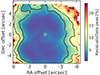 |
Fig. A.1. Residuals of the [OIII] ALUCINE fit (defined as |observations - model|) divided by the observed peak flux, in every spaxel, in percentage. |
Appendix B: Gaussian decomposition of MEGARA lines
See Figs. B.1, B.2, B.3, B.4, and B.5.
 |
Fig. B.1. Gaussian decomposition made by ALUCINE for the Hα line. Top and bottom panels are for narrow and broad component, respectively, while in the three columns, from left to right, are the intensity, velocity, and velocity dispersion maps. The AGN position is marked with a black star symbol, and distances are measured from it. The white circle in the bottom left is the MEGARA seeing conditions. |
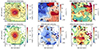 |
Fig. B.3. Same as Fig. B.1, but for the [NII]λλ6548, 6583 doublet. The intensity maps show the sum of the two lines of the doublet, while the kinematics are assumed to be the same between the two lines. The [NII] emission is fitted together with the blended Hα line (Fig. B.1) to properly separate their kinematics. |
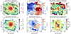 |
Fig. B.4. Same as Fig. B.1, but for the [SII]λλ6716, 6731 doublet. The intensity maps show the sum of the two lines of the doublet, while the kinematics are assumed to be the same between the two lines. |
Appendix C: BPT diagrams of MEGARA lines
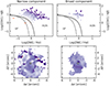 |
Fig. C.1. Diagnostic Baldwin, Phillips, Telervich (BPT) diagram (Baldwin et al. 1981; Veilleux & Osterbrock 1987) of [OIII]/Hβ vs [NII]/Hα line ratios, for the narrow (left panels) and broad (right panels) components of the ionised gas. Solid and dashed black lines are empirical curves derived by Kewley et al. (2001) and Kauffmann et al. (2003), that separate different excitation mechanisms, marked on the plots as SF (star formation) and AGN. The spaxels are coloured depending on their distance from the separation lines, and are plotted with the same colours in the spatially resolved maps (bottom panels). The black star marks the AGN position. |
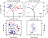 |
Fig. C.2. Same as Fig. C.1, but for the [OIII]/Hβ vs [SII]/Hα. The different excitation mechanisms are marked on the plots as SF (star formation), Sy (Seyfert), and LINER (low-ionisation nuclear emission-line region), with separation lines from Veilleux & Osterbrock (1987). |
 |
Fig. C.3. Same as Fig. C.1, but for the [OIII]/Hβ vs [OI]/Hα. The different excitation mechanisms are marked on the plots as SF (star formation), Sy (Seyfert), and LINER (low-ionisation nuclear emission-line region), with separation lines from Veilleux & Osterbrock (1987). |
Appendix D: Mean velocities radial profiles of all MEGARA lines
See Fig. D.1.
All Tables
All Figures
|
Fig. 1. Optical and molecular views of NGC 5506. Top: HST/F606W image of NGC 5506 from Malkan et al. (1998). The black rectangle identifies a region of 15.3″ × 5.1″ (corresponding to 1.9 × 0.6 kpc2). Bottom: ALMA CO(3 − 2) intensity, velocity and velocity dispersion maps, clipped at a signal-to-noise ratio of 3. The contours are between 10−3 and 10−1 Jy km s−1 (with 0.5 dex steps) for the intensity map, between 1700 and 2000 km s−1 (with 75 km s−1 steps) for the velocity map, and between 10 and 90 km s−1 (with 20 km s−1 steps) for the velocity dispersion map. North is up and east is left, and offsets in the ALMA maps are measured relative to the 870 μm continuum peak (as in García-Burillo et al. 2021), marked with a star symbol in every panel. The ALMA beam (0.21″ × 0.13″) appears in every bottom panel as a black ellipse in the lower left. |
| In the text | |
|
Fig. 2. Optical image and spectra of the central region of NGC 5506. Top panel: GTC/MEGARA [OIII] (λe = 5007 Å, in orange) and CO (λe = 870 μm, in blue) contours over the HST/F606W image of NGC 5506 (Malkan et al. 1998). The [OIII] contour levels, from the single-component Gaussian fit, have a logarithmic spacing from 3σ to 80% of the peak intensity in steps of 0.5 dex, while the CO(3 − 2) contours are the same of Fig. 1. The white star symbol is the AGN position, as determined in Sect. 2.2. The black and white squares are the nuclear region, with size 1.8 arcsec ∼225 pc, observed by X-shooter (see Davies et al. 2020), and the MEGARA FoV (12.5″ × 11.3″ ∼ 1.5 kpc × 1.4 kpc), respectively. The white circle in the bottom left is the MEGARA seeing conditions (diameter 0.9″). Bottom panel: left and right panels contain the spectra (integrated within the MEGARA FoV) revealed with the MEGARA LR-B and LR-R gratings, respectively, with names of identified emission lines and doublets. The inset is the zoom-in of a [OIII] line (after continuum subtraction): the blue shadings are the observed spectra of the MEGARA FoV and of the nuclear region, the black dashed lines are the fits with a single Gaussian. The inset axes have the same units of the outer panel. |
| In the text | |
|
Fig. 3. Visual extinction map of the MEGARA FoV, calculated from the Hα/Hβ ratio and with RV = 3.1 (Cardelli et al. 1989). The white star symbol is the AGN position, and distances are relative to it. The dashed black line is our fiducial major kinematic axis with PA = 265° (see Sect. 4). The white circle in the bottom left is the MEGARA seeing conditions. |
| In the text | |
|
Fig. 4. ALMA CO(3 − 2) PV diagrams generated with 3DB along the kinematic major (top panel) and minor (bottom panel) axes. The grey scale and blue contours are the ALMA CO(3 − 2) observations > 3σ, while the red contours are the 3DB rotating disc model (without a radial velocity component). The yellow dots are the fitted rotation curve. The approximate eastern, western, southern, and northern directions are marked in the panels. |
| In the text | |
|
Fig. 5. Best-fit model and residuals (i.e. observation minus the model) obtained with 3DB for the rotating disc with a radial velocity component. Top and bottom panels show the mean velocity field and the velocity dispersion field of CO(3 − 2), respectively. In the first panel, vsys = 1872 km s−1 has been subtracted from the model velocities. Velocity contours (top panels) are at −50 and 50 km s−1 (solid) and at 0 km s−1 (dotted), while dispersion contours (bottom panels) are at −50, −25, 25, and 50 km s−1 (solid) and at 0 km s−1 (dotted). The dashed black line in the first panel is the kinematic major axis with PA = 265°. The ALMA beam appears in every panel as a black ellipse in the bottom left. |
| In the text | |
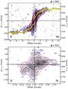 |
Fig. 6. Same as Fig. 4, but for the 3DB run with a radial velocity component. |
| In the text | |
|
Fig. 7. Relative velocities of CO(3 − 2) along the minor axis, extracted and averaged from a slit width of 3 pixels (corresponding to a projected width of 0.09″). The blue circles are the observed values, not weighted for the emitted flux. The green and red lines are the 3DB models with and without a radial velocity component. |
| In the text | |
|
Fig. 8. Radial profiles of the molecular gas derived with 3DB. From top to bottom: the CO(3 − 2) surface density, the rotational velocity (same as the yellow dots in the top panel of Fig. 6), the velocity dispersion and the outflow velocity, all as a function of deprojected distance from the AGN (on the plane of the galaxy). The dashed black line in the bottom panel is the zero line, dividing between ouflow ( |
| In the text | |
|
Fig. 9. Molecular gas mass outflow rate as a function of the deprojected distance from the AGN (on the plane of the galaxy). The molecular gas mass includes the helium contribution. The blue dots correspond to the values computed with the 3DB model radial velocities and CO(3 − 2) intensities of Fig. 8. The blue shading and errorbars represent the variation in r31 and XCO (see text for details). The red dashed line is the integrated mass outflow rate, 8 ± 3 M⊙ yr−1, with the shaded yellow region representing its uncertainty. |
| In the text | |
|
Fig. 10. [OIII] double Gaussian fit made with ALUCINE. Top and bottom rows are for the narrow and broad component, respectively. From left to right, the three columns show the intensity, velocity, and velocity dispersion of both components. The AGN position is marked with a black star symbol, and distances are measured from it. The white circle in the bottom left of each panel is the MEGARA seeing conditions. The velocity panels (central column) show the PA = 265° and 355° dashed black lines, and two black rectangles that highlight the northern and southern edges of the velocity field. |
| In the text | |
|
Fig. 11. PV diagrams of the observed [OIII] (λe = 5007 Å) line, clipped at 3σ, along major (top panel) and minor (bottom panel) kinematic axes, with PA = 265° and 355°, respectively. Contours are at [10, 30, 100, 300, 1000]σ. The vertical dashed line is the AGN position, and the horizontal dashed line is the systemic velocity |
| In the text | |
|
Fig. 12. Observed spectra (continuum-subtracted) of the [OIII]λ5007 line at three locations along the kinematical minor axis (PA = 355°). In green, blue, and red shadings, the spectra extracted within the nuclear region (black square in Fig. 2), the southern region, and the northern region (black rectangles in Fig. 10), respectively. With the same colours, the lines are the ALUCINE two-component fits for the same regions. Note that for the nuclear and southern regions a third component would be needed to fit the residual blueshifted and redshifted components, respectively. The nuclear spectrum is multiplied by a 0.2 factor for a better comparison. The vertical dashed line is the redshifted (with |
| In the text | |
|
Fig. 13. Non-parametric velocity components for the [OIII] line. The top panels show, from left to right, the peak velocity vp, the broad velocity Δv, and the 80% width W80. The bottom panels show, from left to right, the velocity at the 2nd flux percentile (v02), at the 98th (v98), and the positive or negative velocities that have the maximum absolute value between these two (for every spaxel), which is our estimate for the outflow velocity vout. The white star symbol marks the AGN position, and the dashed black line in the top-left panel is the kinematic major axis (PA = 265°). The white circle in the bottom left of each panel is the MEGARA seeing conditions. Velocities in all the panels are in km s−1. |
| In the text | |
|
Fig. 14. Radial profiles for the different mean velocities of the [OIII] line, all as a function of the projected distance from the AGN. Panels show, from top to bottom: the rotational velocity vrot along the kinematic axis, the broad velocity Δv, the 80% width W80, and our estimate for the mean outflow velocity of the ionised gas |
| In the text | |
|
Fig. 15. From left to right: outflowing [OIII] ionisation parameter log U, electron density ne, and mass |
| In the text | |
|
Fig. 16. Radial profile of the ionised mass outflow rate |
| In the text | |
|
Fig. 17. Coloured map of the ionised mass outflow rate, with contours of observed CO(3 − 2) velocity dispersion (as Fig. 1, bottom panel), at 30 and 50 km s−1 in light and dark blue, respectively. The two black circles have a radius of 100 and 250 pc (i.e. ∼0.8 and 2 arcsec, respectively) from the white star symbol, which marks the AGN position. The dashed line is the kinematic major axis. The white circle in the bottom right is the MEGARA seeing conditions. |
| In the text | |
|
Fig. 18. Scenario (not to scale) for the intersection between the molecular disc (the red and blue ellipse) and the ionisation bicone. In the disc of the galaxy, traced by the molecular gas, we mark the AGN position (white star) and the proposed interactions between the two gas phases (black asterisk symbols). The 300-pc radio (at 8.46 GHz) and soft X-ray (below 1 keV) emission is depicted in yellow. Along the ±5″ lines of sight, we draw clouds on the edge of the bicone, colour-coded depending on whether the gas is blueshifted or redshifted. |
| In the text | |
|
Fig. 19. Same as Fig. 17 but with the Schmitt et al. (2001) 3.6 cm VLA contours, at log(Sν/Jy beam−1) = (−4, −3.5, −3, −2.5, −2), in black. The black circle in the bottom right is the MEGARA seeing conditions, with the VLA beam ellipse within it in white. |
| In the text | |
|
Fig. 20. Outflow momentum rate divided by the AGN radiation momentum rate Lbol/c (also called wind momentum load) as a function of the outflow velocity vout for the molecular gas (in blue), the ionised gas (in orange), and the UFO (in green). |
| In the text | |
|
Fig. A.1. Residuals of the [OIII] ALUCINE fit (defined as |observations - model|) divided by the observed peak flux, in every spaxel, in percentage. |
| In the text | |
|
Fig. B.1. Gaussian decomposition made by ALUCINE for the Hα line. Top and bottom panels are for narrow and broad component, respectively, while in the three columns, from left to right, are the intensity, velocity, and velocity dispersion maps. The AGN position is marked with a black star symbol, and distances are measured from it. The white circle in the bottom left is the MEGARA seeing conditions. |
| In the text | |
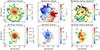 |
Fig. B.2. Same as Fig. B.1, but for the Hβ line. |
| In the text | |
|
Fig. B.3. Same as Fig. B.1, but for the [NII]λλ6548, 6583 doublet. The intensity maps show the sum of the two lines of the doublet, while the kinematics are assumed to be the same between the two lines. The [NII] emission is fitted together with the blended Hα line (Fig. B.1) to properly separate their kinematics. |
| In the text | |
|
Fig. B.4. Same as Fig. B.1, but for the [SII]λλ6716, 6731 doublet. The intensity maps show the sum of the two lines of the doublet, while the kinematics are assumed to be the same between the two lines. |
| In the text | |
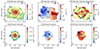 |
Fig. B.5. Same as Fig. B.1, but for the [OI]λ6300 line. |
| In the text | |
|
Fig. C.1. Diagnostic Baldwin, Phillips, Telervich (BPT) diagram (Baldwin et al. 1981; Veilleux & Osterbrock 1987) of [OIII]/Hβ vs [NII]/Hα line ratios, for the narrow (left panels) and broad (right panels) components of the ionised gas. Solid and dashed black lines are empirical curves derived by Kewley et al. (2001) and Kauffmann et al. (2003), that separate different excitation mechanisms, marked on the plots as SF (star formation) and AGN. The spaxels are coloured depending on their distance from the separation lines, and are plotted with the same colours in the spatially resolved maps (bottom panels). The black star marks the AGN position. |
| In the text | |
|
Fig. C.2. Same as Fig. C.1, but for the [OIII]/Hβ vs [SII]/Hα. The different excitation mechanisms are marked on the plots as SF (star formation), Sy (Seyfert), and LINER (low-ionisation nuclear emission-line region), with separation lines from Veilleux & Osterbrock (1987). |
| In the text | |
|
Fig. C.3. Same as Fig. C.1, but for the [OIII]/Hβ vs [OI]/Hα. The different excitation mechanisms are marked on the plots as SF (star formation), Sy (Seyfert), and LINER (low-ionisation nuclear emission-line region), with separation lines from Veilleux & Osterbrock (1987). |
| In the text | |
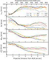 |
Fig. D.1. Same as Fig. 14, but for all the ionised gas emission lines. |
| In the text | |
Current usage metrics show cumulative count of Article Views (full-text article views including HTML views, PDF and ePub downloads, according to the available data) and Abstracts Views on Vision4Press platform.
Data correspond to usage on the plateform after 2015. The current usage metrics is available 48-96 hours after online publication and is updated daily on week days.
Initial download of the metrics may take a while.