| Issue |
A&A
Volume 699, July 2025
|
|
|---|---|---|
| Article Number | A83 | |
| Number of page(s) | 21 | |
| Section | Extragalactic astronomy | |
| DOI | https://doi.org/10.1051/0004-6361/202453291 | |
| Published online | 30 June 2025 | |
Molecular gas excitation and outflow properties of obscured quasars at z ∼ 0.1
1
Instituto de Astrofísica de Canarias, Calle Vía Láctea, s/n, E-38205 La Laguna, Tenerife, Spain
2
Departamento de Astrofísica, Universidad de La Laguna, E-38206 La Laguna, Tenerife, Spain
3
Observatorio Astronómico Nacional (OAN-IGN)-Observatorio de Madrid, Alfonso XII, 3, 28014 Madrid, Spain
4
Instituto de Física Fundamental, CSIC, Calle Serrano 123, 28006 Madrid, Spain
5
Dipartimento di Fisica e Astronomia, Università di Firenze, Via G. Sansone 1, 50019 Sesto F.no (Firenze), Italy
6
INAF – Osservatorio Astrofisico di Arcetri, largo E. Fermi 5, 50127 Firenze, Italy
7
INAF Istituto di Astrofisica e Planetologia Spaziali, Roma, Italy
⋆ Corresponding author: anelise.audibert@iac.es
Received:
4
December
2024
Accepted:
5
May
2025
To investigate the impact of winds and jets with a low to moderate power on the cold molecular gas reservoirs of active galactic nuclei (AGN), we present observations with a high angular resolution with ALMA CO(2–1) and CO(3–2) of a sample of six type 2 quasars (QSO2s) at z ∼ 0.1 from the quasar feedback (QSOFEED) sample. We used spatially resolved molecular line ratio maps, defined as R32 ≡ L′CO(3 − 2)/L′CO(2 − 1), and kinematic modeling to constrain the changes in the gas excitation and to identify gas outflows, respectively. The molecular outflows are co-spatial with regions with R32 > 1, indicating a higher temperature than in the disks and the presence of optically thin gas in the outflows. Considering more and less conservative scenarios to measure the outflow properties, we find mass outflow rates of 5 ≲ Ṁ ≲ 150 M⊙ yr−1, which is much lower than those expected from their AGN luminosities of ∼1045.5 − 46 erg s−1, based on scaling relations from the literature. The outflow kinetic energies might be driven by the combined action of jets and radiation pressure winds, and the radiative coupling efficiencies (ϵAGN ≡ Ėout/Lbol) range from 10−6 < ϵAGN < 10−4 and the jet coupling efficiencies (ϵjet ≡ Ėout/Pjet) from 10−3 < ϵAGN < 10−2. A linear regression including the six QSO2s follows the locus of ϵjet ∼ 0.1%, although we found no strong correlation because of the small-number statistics. Our results provide further evidence that AGN-driven jets/winds disturb the molecular gas kinematics and excitation within the central several kiloparsec of the galaxies. The coupling between compact jets and the interstellar medium might be relevant to AGN feedback, even in the case of radio-quiet galaxies, which are more representative of the AGN population. Finally, the warm (H2) and cold (CO) molecular gas phases seem to be tracing the same outflow. The main distinction between them is the mass they carry, while the warm ionized outflows ([OIII]) do not seem to be another face of the same outflow, as their orientation, velocity, and radius are different.
Key words: ISM: jets and outflows / galaxies: active / galaxies: jets / galaxies: kinematics and dynamics / quasars: emission lines
© The Authors 2025
 Open Access article, published by EDP Sciences, under the terms of the Creative Commons Attribution License (https://creativecommons.org/licenses/by/4.0), which permits unrestricted use, distribution, and reproduction in any medium, provided the original work is properly cited.
This article is published in open access under the Subscribe to Open model. Subscribe to A&A to support open access publication.
1. Introduction
Active galactic nuclei (AGN) are understood today as events in the lifecycle of a galaxy (Harrison & Ramos Almeida 2024) because of their short and episodic nature (0.1–100 Myr, Martini et al. 2004; Hickox et al. 2014; King & Nixon 2015; Schawinski et al. 2015). The accretion of matter onto the supermassive black holes (SMBHs) in the centers of galaxies and the subsequent release of radiation and kinetic energy in the form of outflows profoundly influence the surrounding interstellar medium (ISM) and galactic-scale gas reservoirs (e.g. Veilleux et al. 2020; Valentini et al. 2020; García-Burillo et al. 2021, 2024; Mandal et al. 2021; Ward et al. 2024; Ramos Almeida et al. 2022, hereafter RA22). AGN feedback plays a pivotal role in shaping the evolution of massive galaxies by regulating the growth of their SMBHs and regulating the star formation within their host galaxies (e.g. Croton et al. 2006; Di Matteo et al. 2008; Harrison 2017; Nelson et al. 2019; Harrison & Ramos Almeida 2024).
It is widely recognized that AGN feedback operates through two primary channels: the quasar/radiative and the radio/kinetic mode (Fabian 2012; Dubois et al. 2016). The quasar mode predominates in luminous AGN with high accretion rates, where radiation-driven wide-angle winds are launched, and it commonly manifests itself in high-redshift young quasars (King 2003; Zubovas & King 2012; Bieri et al. 2017). The radio mode is often associated with collimated relativistic jets that are primarily observed in low-luminosity AGN with low accretion rates. The kinetic energy deposit by the jets into the galaxies delays cooling flows from the intracluster/intragroup medium and prevents the formation of extremely massive galaxies (Fabian 2012; McNamara & Nulsen 2012; Bourne & Sijacki 2017; Bourne & Yang 2023).
Despite this dichotomy between the feedback modes, kiloparsec-scale radio jets of a low to moderate luminosity (log P1.4 GHz < 1024 W Hz−1) are starting to be recognized as a potential driver of multiphase outflows in radiatively efficient radio-quiet quasars. For example, in the case of optically selected type 2 quasars (QSO2s; e.g., Reyes et al. 2008), compact radio jets are associated with morphologically and kinematically distinct features in the ionized and molecular gas, such as outflowing bubbles and increased turbulence, which reveal the jet-gas interactions on galactic scales (e.g., Mullaney et al. 2013; Villar-Martín et al. 2017; Ramos Almeida et al. 2022; Girdhar et al. 2022; Audibert et al. 2023; Venturi et al. 2023; Speranza et al. 2024; Ulivi et al. 2024). Simulations showed that confined low-power jets (Pjet ∼ 1043 − 44 erg s−1) are indeed able to induce feedback into the ISM in the form of local turbulence and shocks that alter the physical conditions of the surrounding gas (Mukherjee et al. 2018; Meenakshi et al. 2022; Talbot et al. 2022).
Hosting ubiquitous galactic-scale multiphase outflows, QSO2s offer an excellent opportunity to study the effects of quasar- and radio-mode AGN feedback on the host galaxy properties. In particular, the impact of AGN on the molecular gas content of the ISM plays a critical role for the galaxy evolution because in the nearby Universe, the cold molecular gas phase appears to carry the bulk of the outflow mass budget, while the ionized gas phase only carries a small fraction of the total outflowing mass, at least for low- to intermediate- AGN luminosities (Lbol < 1046 erg s−1 Fiore et al. 2017; Fluetsch et al. 2019). Most of the molecular outflows that were traced using CO, however, were detected in low-luminosity AGN (i.e., Seyfert galaxies; e.g. see Combes et al. 2013; Audibert et al. 2019, 2021; García-Burillo et al. 2019, 2021; Feruglio et al. 2020; Zanchettin et al. 2021) and in ultraluminous infrared galaxies (ULIRGs; e.g. Feruglio et al. 2010; Cicone et al. 2014; García-Burillo et al. 2015; Pereira-Santaella et al. 2018; Fluetsch et al. 2019; Lamperti et al. 2022; Holden et al. 2024), and until recently, the high-luminosity regime was scarcely observed in the molecular gas phase.
In the quasar regime of AGN luminosities (LAGN ≳ 1045 − 46 erg s−1), where most massive outflows are expected in the molecular phase, recent observational results revealed a different scenario. In a sample of seven QSO2s at redshifts z ∼ 0.1 observed with the Atacama Large Millimeter/submillimeter Array (ALMA) in CO(2–1) at 0 2 (400 pc), RA22 reported cold molecular outflows in the five QSO2s with a CO(2–1) detections. The molecular mass outflow rates (Ṁ) are lower than those expected from their AGN luminosities according to empirical scaling relations (Cicone et al. 2014; Fiore et al. 2017; Fluetsch et al. 2019). The measured outflow mass rates and velocities of Ṁout ∼ 8−16 M⊙, yr−1 and vout ∼ 200–350 km s−1 (RA22) are intermediate between those of the molecular outflows detected in Seyfert galaxies (Ṁ ∼ 0.3–5 M⊙ yr−1, vout ∼ 90–200 km s−1) and in ULIRGs hosting AGN (Ṁ ∼ 60–400 M⊙ yr−1, vout ∼ 600–1200 km s−1) (see RA22 for a discussion of the different outflows properties in these systems).
Additionally, molecular outflows with sizes of a few kiloparsecs were detected in four QSO2s with redshifts z < 0.2 using CO(3–2) observations at 0 3–0
3–0 6 spatial resolution, and in the case of two of the targets, molecular gas was detected around the 5–13 kpc scale radio lobes of these radio-quiet sources (Girdhar et al. 2024). In the case of the Teacup, which is a radio-quiet quasar hosting a compact jet that is almost coplanar with the cold molecular disk, the bulk of the molecular outflow is mostly detected in the direction perpendicular to the compact radio jet (∼1 kpc in size Audibert et al. 2023, hereafter AA23). This is traced by the high CO velocity dispersion and also by a high L′CO(3 − 2)/L′CO(2 − 1) line ratio (R32) perpendicular to the radio jet. A comparison with the tailored simulations of jet-ISM interaction first presented by Mukherjee et al. (2018) and Meenakshi et al. (2022) supported a scenario in which the radio jet compresses and accelerates the molecular gas to drive a lateral outflow that shows enhanced turbulence and gas excitation perpendicular to the radio jet in the Teacup (AA23). Similar enhanced velocity dispersion perpendicular to jets was observed in CO(3–2) for another QSO2 by Girdhar et al. (2022) and in a few QSO2s in the ionized gas traced by [OIII] (Venturi et al. 2023; Speranza et al. 2024; Ulivi et al. 2024). Altogether, these results suggest that other factors in addition to the AGN luminosity, such as the jet power, the spatial distribution of the dense gas in the ISM, and the coupling between jets and the dense gas, might also be relevant for driving more or less massive molecular outflows (RA22, AA23).
An alternative approach for discerning the imprints of AGN feedback on molecular gas involves examining various CO transitions or CO spectral line energy distributions (SLEDs). This provide insight into the mechanisms driving molecular gas excitation. The CO excitation is suggested to be driven by photodissociation regions (PDRs) and X-ray-dominated regions (XDRs) and displays a wide range of temperature and gas densities (Hollenbach & Tielens 1999; Meijerink et al. 2007; Esposito et al. 2022, 2024). Processes related to AGN activity, such as shocks induced by jets/outflows and by X-ray emission, can enhance the gas emission, especially at high-J transitions (e.g., van der Werf et al. 2010; Mingozzi et al. 2018; Vallini et al. 2019). Recently, Molyneux et al. (2024) analyzed multiple integrated CO transitions in a sample of 17 QSO2s at z < 0.2 that were observed with the Atacama Compact Array (ACA) or the Atacama Pathfinder EXperiment telescope (APEX). Their CO SLEDs indicated that AGN feedback does not seem to exert a substantial influence on the molecular gas content and excitation on global galaxy scales. Instead, the authors proposed that its effects might be observed on localized and more nuclear scales that cannot be resolved with the ACA and APEX observations. The spatially resolved line ratios indeed offer a means to explore these scales and unveil localized alterations in gas excitation that are attributable to jets and/or outflows, as evidenced by elevated values of the low-J CO line ratios observed in certain jetted Seyfert/radio galaxies (e.g., García-Burillo et al. 2014; Dasyra et al. 2016; Oosterloo et al. 2017, 2019; Fotopoulou et al. 2019; Ruffa et al. 2022). Investigations into local variations in gas conditions due to compact jets or AGN-driven outflows in radio-quiet quasars using spatially resolved molecular line ratios, however, have thus far been limited to the study of the Teacup galaxy (AA23).
We present an analysis of the molecular gas kinematics and excitation of six QSO2s that are part of the Quasar Feedback (http://research.iac.es/galeria/cra/qsofeed/) sample, using ALMA CO(3–2) observations at 0 25−0
25−0 6 (450−1300 pc) resolution, in addition to the CO(2–1) data at 0
 2 resolution first presented by RA22. The observations used in this work and the data reduction are described in Section 2, and the morphology, kinematics, and CO line ratios are presented in Section 3. We discuss the dependence of the molecular outflow energetics on the AGN, radio jet, and host galaxy properties in Section 4, and the main conclusions are drawn in Section 5. We adopt a flat ΛCDM cosmology with H0 = 70 km s−1 Mpc−1, ΩM = 0.3, and ΩΛ = 0.7.
2. Sample and observations
This work is part of the QSOFEED project (Ramos Almeida et al. 2022, Ramos Almeida et al. 2025; Pierce et al. 2023; Bessiere et al. 2024; Speranza et al. 2024), whose aim is to characterize and understand the direct impact of AGN feedback on the central region of nearby quasar host galaxies. The QSOFEED sample was drawn from the compilation of narrow-line AGN by Reyes et al. (2008) and were selected based on their [OIII] luminosites (L[OIII] > 108.5 L⊙) and redshits (z < 0.14), resulting in a sample of 48 QSO2s with stellar masses ranging from 1010.7 to 1011.6 M⊙. The redshift cut was set to detect 2.12 μm H2 emission line in the near-infrared (NIR; see for instance Ramos Almeida et al. 2017, 2019; Speranza et al. 2022; Zanchettin et al. 2025) from the ground. The ionized outflow properties and stellar populations of the full sample are reported in Bessiere et al. (2024) and the optical morphologies, which are dominated by galaxy interactions, in Pierce et al. (2023).
The subset of six quasars presented here consist of the five QSO2s with CO(2–1) ALMA observations at 0 2 spatial resolution analysed in RA22 plus J1347+1217 (also known as 4C12.50 and F13451+1232), a ULIRG with the largest radio luminosity in the QSOFEED sample. The main properties of the selected six QSO2s are listed in Table 1. In this work, we re-analysed the CO(2–1) data of the five QSO2s presented in RA22 together with archival ALMA CO(3–2) observations at 0
 25−0
25−0 6 resolutions (corresponding to physical scales of 450 pc to 1.1 kpc at the redshifts of our targets), and in the case of J1347+1217, we use publicly available CO(2–1) and CO(3–2) ALMA observations at similar angular resolution, first presented in Fotopoulou et al. (2019) and Lamperti et al. (2022).
Main properties of the quasars.
The ALMA observations of the CO(2–1) and CO(3–2) emission lines were observed in bands 5, 6, and 7. The CO(2–1) observations and data reduction are described in detail in RA22, and those of J1347+1217 in Lamperti et al. (2022). We retrieve the CO(3–2) observations from the ALMA archive for five of the targets, as no CO(3–2) observations are available for J1509+0434. These observations are part of different projects, whose details, including principal investigator (PI) name, project ID, synthesized beam, maximum recoverable scale (MRS), and root mean square (rms) noise are listed in Table 2.
Properties of the ALMA observations.
The CO(3–2) data were calibrated using the appropriate CASA software version (Martini et al. 2004) in the pipeline mode and using the standard flux, bandpass, and phase calibrators. Once calibrated, the imaging and cleaning were performed with the task TCLEAN. The spectral line map was obtained after subtracting the continuum in the uv-plane using the tasks UVCONTSUB and a 0th order polynomial in the channels free from emission lines. The CO(3–2) data cubes were produced with spectral resolutions listed in Table 2 and using Briggs weighting mode and a robust parameter set to 0.5 in order to achieve the best compromise between resolution and sensitivity. In the case of J1347, the CO(3–2) data reduction was performed by Fotopoulou et al. (2019) using similar CASA routines. Finally, the datacubes were corrected for primary beam attenuation. In order to study the line ratios and compare the CO(2–1) to the new CO(3–2) datacube, we regridded the CO(2–1) data to the same pixel scale of the CO(3–2) and then convolved it to the same common beam sizes.
The auxiliary radio data used here are the 6 GHz Very Large Array (VLA) C-band observations of J1010, J1100, J1356, and J1430 first presented in Jarvis et al. (2019, 2021). These data were obtained in two different configurations: the high-resolution (0 25, HR) A-array and the low-resolution (1
 0, LR) B-array maps. In the case of J1100, we also consider the e-MERLIN observations at 1.5 GHz obtained at a 0
 3 resolution from Jarvis et al. (2019). In the case of J1347 (4C12.50), we used the 15 GHz observations from the Very Long Baseline Array (VLBA), retrieved from the NASA/IPAC Extragalactic Database (NED) and presented in Kellermann et al. (2004). Finally, no VLA observations are yet available for J1509. The main properties of the radio observations used in this work are listed in Table A.1 of Appendix A.
3. Results and analysis
3.1. Moment maps of the CO(3–2) emission
The properties of the molecular gas traced by the CO(2–1) emission are presented in RA22 for five of the QSO2s and in Lamperti et al. (2022) for J1347. In order to show the distribution of the CO(2–1) gas from a slightly different perspective and to allow a comparison with the CO(3–2) emission, we computed the peak-intensity maps of CO(2–1), which are shown in Figure 1. As discussed in RA22, the CO(2–1) emission of the QSO2s reveals a variety of morphologies: from spiral arms in the case of the J1100 and J1509 to double-peaked structures in J1010, J1347, and J1430, and a central concentration in J1356 together with a west arc that is part of an on-going merger. One of the advantages of the peak maps is that clumpy and narrow structures can be better seen, since they are smoothed in the integrated-intensity (moment-0) maps. The CO(2–1) peak maps clearly exhibit the double-peaked features in J1010, J1347, and J1430 (the merging/interacting systems) but also enhance conspicuous regions in the spiral systems, that appear diluted in the integrated-intensity maps. The CO(2–1) moment-0 map of J1100, shown in RA22, revealed only some of the clumps mainly along the bar, while the peak map shows clumps spread along the two spiral arms. In the case of J1509, the CO(2–1) moment-0 map shows centrally concentrated gas, and the CO(2–1) peak map reveals several clumpy structures within the central region.
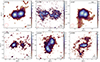 |
Fig. 1. ALMA CO(2–1) peak-intensity maps of the six QSO2s. The color bars indicate the scales of the flux density in mJy. The horizontal black lines indicate the physical scales for each galaxy, and the beam sizes are shown in the bottom left corner of each panel as red ellipses. The CO(2–1) distribution presents a variety of morphologies, such as spiral arms, double peaks, and merger signatures. East is to the left, and north is up. |
Using the CO(3–2) data cubes, we computed the peak-intensity, integrated-intensity (moment-0), intensity-weighted velocity field (moment-1), and velocity dispersion (moment-2) maps, which are shown in Figure 2. The moment maps were created using the CASA task immoments and a 3σrms clipping. The CO(3–2) maps of J1430 (Teacup) were presented in Appendix A of AA23, but they are included here for comparison with those of the other QSO2s. Double-peaked morphologies1 are also seen in the CO(3–2) peak-intensity maps (left panels of Figure 2) for the interacting quasars J1010, J1347, and J1430. The CO(3–2) distribution shown in the moment-0 maps (central-left panels) is more compact than the CO(2–1) in the cases of J1010 and J1356, although the western arc part of the merger in the latter is less noticeable in CO(3–2) than in CO(2–1). For J1347, the coarser resolution of the CO(3–2) data makes the southern part of the merger clearly detected. In the case of J1100, the bar and spiral arms are prominent in CO(3–2), similar to the morphology seen in CO(2–1).
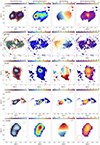 |
Fig. 2. Moment maps of the CO(3–2) emission for the QSO2s. From left to right, the panels correspond to the peak intensities (in mJy units), the integrated intensity (moment 0, in Jy beam−1 km s−1 units), the intensity-weighted velocity field (moment 1, in km s−1), and the velocity dispersion (moment 2, in km s−1), respectively. East is to the left, and north is up. The red ellipses in the bottom left corner of the velocity dispersion maps indicate the beam sizes. The black stars show the nuclei, defined as the peak of the 220 GHz continuum as in RA22. For the cases of J1347 and J1356, a secondary nucleus (blue star) is identified in the optical and/or with ALMA continuum to the East and South directions, respectively. Green contours on the left panels indicate the ∼0 |


The integrated-velocity field maps (moment 1) in the middle-right panels of Figure 2 show a rotation pattern for the main disk of the five quasars displayed, with projected velocities of v ≈ ±220 km s−1, except for J1010 that shows a higher amplitude up to v ≈ ±300 km s−1. We note that the interacting western arc in J1356 has blueshifted velocity components, while the southern region part the merging system in J1347 shows redshifted velocities. The fact that the velocity pattern of the merging regions coincides with the blue(red)shifted sides of the main disk indicates that the gas there is starting to settle into them.
In the right panels of Figure 2 we present the CO(3–2) velocity dispersion (moment-2) maps. The central velocity dispersions are typically vdisp ≳ 100 km s−1 in the nucleus of the galaxies, with decreasing values outwards. J1356 shows high values of vdisp, of ∼200 km s−1, which are larger than the maximum value of ∼160 km s−1 measured from CO(2–1) by RA22. The same is observed for the barred spiral J1100, where the CO(3–2) and CO(2–1) maximum dispersion values are ∼160 km s−1 and ∼120 km s−1, respectively. The opposite is found for J1010, since the CO(3–2) vdisp in the nucleus peaks at 100 km s−1, smaller then the 120 km s−1 measured for the CO(2–1). The velocity dispersion values of CO(3–2) for J1347 are centrally peaked at ∼140 km s−1, same as those reported in CO(2–1) by Lamperti et al. (2022). There is a difference in the southern merging region, where CO(2–1) exhibits low values (< 40 km s−1), indicative of gas settling in the merger (see the CO(2–1) velocity dispersion map in Figure 3), while in CO(3–2) the same region shows values of up to 160 km s−1. We note that higher velocity dispersions measured in CO(3–2) can be due to beam smearing, as these observations have coarser resolution then the CO(2–1) data. Indeed, when convolving to a common resolution the values measured for CO(3–2) and CO(2–1) are more similar.
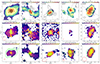 |
Fig. 3. Brightness temperature ratio R32 and CO(2–1) and CO(3–2) velocity dispersion maps. The top panels show the R32 map at the coarser resolution of either CO(2–1) or CO(3–2), with the VLA 6 GHz HR contours overlaid in black (at 4, 8, 16, 32, and 64σrms, with σrms listed in Table A.1 in the appendix, also in Table 3 of Jarvis et al. 2019). For J1100 we present the e-MERLIN observations at 1.5 GHz at a 0 |

3.2. Integrated fluxes and line ratios
We report the integrated fluxes, SCOΔV, detected in CO(2–1) and CO(3–2) in Table 3. To compute the total CO masses, we first convert the integrated flux measurements to CO luminosities L′CO, in units of K km s−1 pc2, using the following equation of Solomon & Vanden Bout (2005):
Integrated properties of the QSO2s and radii of the corresponding regions.
where νobs is the observed frequency of the CO line, in GHz, DL is the luminosity distance of the galaxy, in Mpc, z is the redshift and SCOΔV is the integrated flux in Jy km s−1. The CO transitions can be converted to L′CO(1 − 0) adopting a line ratio, called  . Under the assumption that the gas is thermalized and optically thick, L′CO(3 − 2) = L′CO(2 − 1) = L′CO(1 − 0), and therefore the brightness temperature ratio RJ − 1 = 1.
The molecular masses can be calculated from L′CO(1 − 0) using the CO-to-H2 conversion factor MH2 = αCOL′CO(1 − 0). We adopted the standard Galactic CO-to-H2, conversion factor of αCO = 4.36 M⊙ (K km s−1 pc2)−1 (Tacconi et al. 2013; Bolatto et al. 2013). The molecular masses inferred from the CO(3–2) emission are of the order of (3–4)×109 M⊙ (see Table 3), which are systematically lower than the ones derived using the CO(2–1) observations in RA22 and Lamperti et al. (2022). Both mass estimates were computed under the same assumptions of αCO and thermalized gas R31 = R21 = 1, therefore indicating that the molecular gas in the QSO2s is less excited and has temperature and density conditions below the thermalized limit. Indeed, we derived the integrated R32 line rations, also listed in Table 3, and we find values of R32 < 1. The values derived for the integrated line ratios range 0.22 < R32 < 0.75, with an average value of ⟨R32⟩ = 0.5 ± 0.2, similar to the line ratios typically measured in spiral and disk galaxies (Leroy et al. 2022). In the next section, we present spatially resolved line ratios to examine possible localized changes in the gas conditions of the QSO2s. A discussion of the physical condition of the gas is addressed in Section 4.3.
3.3. Spatially resolved line ratios
The spatial resolution of our ALMA CO(2–1) and CO(3–2) observations allows us to produce spatially resolved line ratio maps, which can provide insights into the changes in gas excitation due to the AGN ionization, jets, and star formation. Line ratio maps allow us to unveil signatures that differentiate outflows from ambient ISM. In Figure 3 we present the R32 maps (top panels) together with the velocity dispersion (bottom panels) of the five quasars, similar to the analysis reported for the Teacup in AA23. The radio continuum emission from the VLA HR data at 6 GHz is indicated as black contours (except for J1100 and J1347, for which we report e-MERLIN data at 1.5 GHz and VLBA data at 15 GHz, respectively). The PA orientation of the radio emission is indicated with black solid lines. The ALMA continuum at either 200 or 300 GHz is shown in blue contours overlaid on the velocity dispersion maps.
The R32 maps shown in the top panels of Figure 3 show higher values in the nuclear region, of R32 ∼ 0.7–0.9, compared to the smaller values found across the CO disks, of R32 ∼ 0.2–0.5. The regions of enhanced R32 are usually co-spatial with those showing high central velocity dispersion in the bottom panels.
No clear trend regarding the orientation of high R32 and velocity dispersion with the PA of the radio jets is found for the QSO2s. Apparent enhanced turbulence and gas excitation perpendicular to the radio jet is only found for the Teacup, as reported in AA23. Tentative perpendicular orientation of the R32 and velocity dispersion is found for J1100, where the PAjet = 175° derived from the e-MERLIN contours is misaligned by ∼135° with the axis of high R32 and dispersion (PA ∼ 40°). The region showing high values of R32 in J1347 appears perpendicular to the orientation of the 100 pc jet, whilst the region of high velocity dispersion is aligned with the jet. For J1010 and J1356, the VLA HR data is unresolved, and therefore the orientation of possible jets (as suggested by the spectral index analysis in Jarvis et al. 2019) is merely indicative and derived from the larger scale radio structures seen in the low-resolution radio images.
Therefore, although some targets exhibit a degree of (anti-) alignment between R32, velocity dispersion, and radio emission, the results are not consistent across the sample. One of the goals of the QSOFEED project is to understand how different outflow, jet, and ISM properties – and their interactions, including orientation and energy exchange among others – shape the observed gas kinematics and excitation. Given the diverse and complex nature of the individual targets, a larger sample is required to explore the broad parameter space and derive more general conclusions.
3.4. Modeling the kinematics of the molecular gas
We analysed the CO(2–1) and CO(3–2) kinematics using the “3D-Based Analysis of Rotating Objects from Line Observations” (3DBAROLO) software by Di Teodoro & Fraternali (2015). 3DBAROLO performs a 3D tilted-ring modeling of the emission line datacubes to derive the parameters that better describe the kinematics of the data. We ran 3DBAROLO on both CO(3–2) and CO(2–1) datacube in order to investigate non circular motions, since the code allows us to infer radial velocities in the fit of the rotation curves.
The center was fixed to the position of the continuum peak at 200 GHz and we allowed 3DBAROLO to fit the inclination, PA, systemic velocity, rotation velocity, and dispersion as free parameters. For the initial guess on the inclination and PA, we used the parameters derived in RA22 and for the case of J1347 in Holden et al. (2024). We then fixed the inclination, PA, and systemic velocity to the average values derived from the first run2 and allow the code to fit only rotation and dispersion. We present the results of the analysis with 3DBAROLO in form of position-velocity diagrams (PVDs) along the major and minor axis of the CO(3–2) disk in Figures 4–7. Since the CO(2–1) 3DBAROLO fits are already shown in detail in RA22, here we just show the results for CO(3–2), although in the right panels of Figures 4–7 we also present the PVDs of the R32 to identify regions having different gas excitation conditions. The R32 PVDs were smoothed using a Gaussian kernel with a σ = 1.5 to reveal intrinsic variations and reduce the noise due to a pixel-by-pixel ratio.
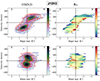 |
Fig. 4. Position-velocity diagrams along the major (top panels) and minor (bottom panels) axis of the of the CO(3–2) emission (left) and the R32 line ratios (right) for J1010. The PVDs were extracted in a slit of 0 |

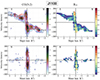 |
Fig. 5. Same as Fig 4, but for J1100. The PVDs were extracted in a slit of 0 |

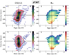 |
Fig. 6. Same as Fig. 4, but for J1347. The PVDs were extracted in a slit of 0 |

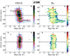 |
Fig. 7. Same as Fig. 4, but for J1356. The PVDs were extracted in a slit of 0 |

In Figure 4 the CO(3–2) PVDs for the quasar J1010 show a clear rotation pattern along the major axis (PA = 288°, or PA = −72°). The 3DBAROLO model is displayed as red contours and it reproduces well rotation up to velocities of ∼300 km s−1, although it cannot fit the high-velocity gas within 0 and 1 5 to the east, which shows velocities of up to −400 km s−1 (see top left panel in Figure 4). This noncircular velocity feature is more clearly visualized in the high velocity map shown in Figure 8 and discussed in Section 4.1. The line ratio PVDs shown on the right panels of Figure 4 have typical values of R32 ∼ 0.8, in agreement with the global ratio derived from the integrated fluxes listed in Table 3. There are several regions, however, that show values R32 > 1, indicating the presence of optically thin gas and/or gas with higher excitation temperatures. These regions with R32 > 1 are distributed all over the minor and major axis slits for the low- and high-velocity components.
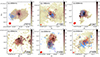 |
Fig. 8. High-velocity flux maps overlaid on the CO velocity dispersion maps for the six QSO2s. The color maps corresponds to the moment 2 of the total CO(2–1) emission at 0 |

The CO(3–2) PVDs for the spiral J1100 are presented in the left panels of Figure 5 and show clear rotation along the major axis (PA = 69°, same as the PA derived for the CO(2–1) line) that is well reproduced by the 3DBAROLO fit shown as red contours, and the typical 0th velocities along the minor axis. In the central region, concentrated in a radius of less than 0 4 (740 pc), the PVDs along the major and minor axes show a large velocity gradient with velocities reaching ±300 km s−1. The 3DBAROLO model reproduces well rotation up to velocities of ∼180 km s−1, but it cannot fit the high velocities in the nuclear region. These high velocity regions coincide with the highest line ratios seen in the R32 PVDs on the right panels of Figure 5, with R32 values between 0.6 and 1.2, higher than the typical values of R32 < 0.5 found along the spiral arms at larger radii. Compared to the integrated value of ⟨R32⟩ = 0.22 in Table 3, this indicates that the global ratio traces mostly the contribution from the galaxy disk.
For the merging galaxy J1347, we show the PVDs in Figure 6. The CO(3–2) along the major axis (top left panel) shows a rotation pattern oriented along the west-east direction (PA = 248°) that can be fit with the 3DBAROLO model up to velocities of ∼300 km s−1. There is a clear excess of blueshifted velocities up to 420 km s−1 in the central to east direction that cannot be fit by rotation. Along the minor axis (PA = −22°, bottom left panel), the high blueshifted velocities are also present, and we can see the contribution from the southern part of the merger mostly in redshifted velocities. The line ratio PVDs (right panels of Figure 6) of the main disk (r < 1″) have values of R32 ∼ 0.8, slightly larger than the global ratio derived from the integrated fluxes of ⟨R32⟩ = 0.69, as listed in Table 3, and values R32 < 0.5 across the southern part of the merger. The regions in which the highly blueshifted velocities lie along the major and minor axes, however, show the highest line ratios, of R32 ∼ 1 − 2, indicating the presence of optically thin/warmer fast gas.
In Figure 7 the CO(3–2) PVDs of J1356 show a less prominent contribution from rotation along the major axis (PA = 110°) for the main galaxy disk (r < 0 5 ≃1.1 kpc) and the system present an overall large velocity dispersion (see Figure 3). The blueshifted velocities seen between 0 and 1″ to the west correspond to the western arc of the merging system. The 3DBAROLO model, displayed as red contours, can reproduce rotation up to velocities of ∼300 km s−1, but it fails to reproduce the high velocity gas at velocities up to ±400 km s−1, mostly detected at redshifted velocities. The line ratio PVDs on the right panels of Figure 7 have typical values of R32 ∼ 0.6 along the main disk (or north nucleus in RA22) and R32 < 0.5 along the western arc, higher than the value derived from the integrated intensities of ⟨R32⟩0.3. One possible reason is that the sensitivity of the CO(2–1) is much better than the CO(3–2), allowing for a clearer detection of the western arm and the southern nucleus of the system (see Appendix D.1 in RA22), while in the shallower CO(3–2) observations only part of the western arm is detected and the southern nucleus is undetected, making the integrated R32 lower. On the other hand, we find R32 values of up to 1.2 in regions that are co-spatial with the redshifted high velocity gas, indicating different excitation conditions there.
The PVDs of CO(2–1), CO(3–2), and R32 of the Teacup (J1430) can be seen in Figure 2 of AA23 and are described in full there. We find values of R32 ∼ 0.4–0.8 across the disk, and the highest values, of up to R32 ∼ 1, in the region occupied by high-velocity blueshifted gas (∼200–350 km s−1) within 0 and 1″ to the south.
The regions of the QSO2s where we detected high velocity gas components and gas excitation differing from ambient gas conditions in the main disks are interpreted as outflowing gas. This interpretation is based on the fact that their kinematics cannot be explained by regular rotation, based on our analysis using 3DBAROLO, and they show higher excitation temperatures than those typically found in the galaxy disks of non-active star-forming galaxies. We note that this is the same outflow definition employed in Ramos Almeida et al. (2022), but adding gas excitation. We note that in the case of the merging galaxies, J1347 and J1356, the observed nonrotational motions could be attributable to merger-induced flows. Numerical simulations suggest, however, that molecular gas velocity dispersions in mergers typically reach only tens of km s−1 (Bournaud et al. 2008, 2011), which is significantly lower than the values that we measure in the QSO2s. Observationally, ALMA CO(3–2) observations of the overlapping region between the merging Antennae galaxies (NGC 4038/39), a prototypical merger, revealed knots of low-velocity dispersion (∼10 km s−1) and maximum values of up to ∼80 km s−1 in supergiant molecular clouds (Whitmore et al. 2014). Considering this, we favor the outflow interpretation to explain the observed kinematics and gas excitation.
3.5. Molecular outflow properties
The determination of the outflow mass rates in the literature is performed using heterogeneous methods. From the observational point of view, it is challenging to obtain a precise determination of the outflow mass, radius, and velocities, all affected by uncertainties. Different methodologies and assumptions can lead to estimates that diverge in more than an order of magnitude (Hervella Seoane et al. 2023; Harrison & Ramos Almeida 2024). For these reasons, here we consider three scenarios for estimating the outflow masses and mass rates, from least to most conservative, following AA23. To measure the fluxes and corresponding masses, we used the CO(2–1) data at the original 0 2 resolution to avoid artefacts or wrong interpretations of the results due to possible beam smearing effects because of the larger CO(3–2) beam size. The only exception is for J1010, in which CO(3–2) was used because it has better spatial resolution (0
 25) than the CO(2–1) data (0
 75).
75).
I) In the first scenario, we assume that all the molecular gas that cannot be reproduced with our rotating disk model is outflowing. Thus, we just integrated the emission from the 3DBAROLO model and subtracted it from the CO(2–1) datacube. We find that for the spirals J1100 and J1509 and the interacting early-type galaxy J1010, most of the CO(2–1) emission can be reproduced with rotation (∼75%), while the mergers J1347 and J1356, and the post-merger system J1430 present more complex kinematics, with J1356 being dispersion-dominated (see Figure C.1 in Appendix C) and therefore rotation accounts for ∼50% of the total CO emission. In this scenario, we adopted an outflow velocity, vout, calculated as the average of the mean redshifted and the mean blueshifted velocity residuals from the 3DBAROLO fit shown in RA22 and in Appendix B, using absolute values. These velocities are in the range 50 < vout < 100 km s−1 (see Table 4).
Outflow measurements derived from the three scenarios proposed for the QSO2s.
II) In the second scenario, we consider that only the gas with the highest velocities is outflowing. The determination of the velocity cut comes from the comparison between the PVDs shown in Figures 4–7 and the 3DBAROLO rotation model, shown in red contours in the same figures. The outflow velocity, vout, is defined as the velocity cut above the maximum rotation velocity that is modeled with 3DBAROLO. To calculate the flux of the high velocity gas, we then created moment-0 maps by selecting only channels above the rotation velocities modeled with 3DBAROLO, shown in Figure 8. In the case of J1010 we only see the blueshifted side of the outflow, reaching velocities up to 300 km s−1 in the corresponding PVD (see Figure 4). The same happens in the case of J1347, based on the detection of high-velocity gas and excitation seen in the PVDs in Figure 6. As for J1356, we only considered the more prominent redshifted velocities seen in the PVDs in Figure 7 that also correspond to the region with high values of R32.
III) The third scenario is a mix of the first two. We assume that all the high-velocity gas is outflowing, but the contribution from rotation is subtracted following a similar approach as in García-Burillo et al. (2019). We first subtracted the contribution of circular motions by de-projecting the one dimensional rotation curve derived with 3DBAROLO to the corresponding velocity field on a pixel by pixel basis. We re-shuffled the channels in order to remove the rotation component from the velocity axis of the CO(2–1) datacube. Then, we created the residual integrated spectrum, resulting in a narrower residual CO profile (i.e., without the rotation component), as the one we presented for the Teacup in Appendix C of AA23. Since this method is suited to optimize the signal-to-noise ratio of the emission associated with noncircular motions, it can reveal high-velocity wings that otherwise are too faint and/or immersed in the total CO profiles to be detected. Using the residual CO profiles, we estimate the flux contribution of the outflowing gas by integrating the flux of the high-velocity gas in the blue and red wings, using the same velocity cut as in Scenario II.
In Table 4 we list the derived outflow integrated intensities (SCO), velocities (vout), and radii (rout) of the QSO2s in each of the three scenarios considered. We note that for J1347 and J1356 we did not measure the outflow fluxes as described in scenarios I and III because they are ongoing mergers with very complex kinematics showing a small contribution from rotation (as discussed in Section 3.4 and Appendix C), and since scenarios I and III depend on the subtraction of the rotation model, respectively, they cannot be performed accurately. Instead, in the case of J1347 we used as the least conservative scenario (Scenario I in Table 4) the recent molecular outflow properties reported by Holden et al. (2024) based on CO(1–0) observations at 0 05 resolution. The CO(1–0) outflow is compact (120 pc) and likely driven by the small scale radio jet detected with VLBI and shown in Figure 3 (Morganti et al. 2013; Holden et al. 2024). As for the most conservative scenario (Scenario III in Table 4), we adopted the upper limit derived by Lamperti et al. (2022) from the CO(2–1) observations at 0
 22 resolution. We note that the CO(3–2) data, first presented in Fotopoulou et al. (2019), show blueshifted velocities of up to ∼400 km s−1 that are not seen in CO(2–1). For this QSO2, however, the high angular resolution CO(1-0) data reported by Holden et al. (2024) were crucial to detect the nuclear outflow of rout ∼ 120 pc, which shows velocities of up to ∼600 km s−1. In the case of J1356, we adopt as the least conservative scenario (Scenario I in Table 4) the outflow properties reported by Sun et al. (2014), based on the CO(3–2) observations, but using an average outflow velocity of 400 km s−1 instead of the maximum outflow velocity adopted by these authors, of vout = 500 km s−1. The most conservative scenario (Scenario III in Table 4) in the case of J1356 corresponds to the outflow properties reported by RA22, which were calculated considering just outflowing gas along the kinematic minor axis of the galaxy.
We computed the outflow masses from the integrated flux measurements of the outflows. First, the integrated fluxes were converted to CO luminosities, LCO(2 − 1)′, in units of K km s−1 pc2 using Equation (3) of Solomon & Vanden Bout (2005) and then translated into masses using the CO-to-H2 (αCO) conversion factor MH2 = αCOR12L′CO(2 − 1). Under the assumption that the gas is thermalized and optically thick, the brightness temperature ratio R12 = LCO(1 − 0)′/LCO(2 − 1)′ = 1. We adopted the conservative value of αCO = 0.8, commonly used to derive outflow masses (see RA22 and references therein). The values of the outflow masses derived from each scenario are listed in Table 4.
To compute outflow mass rates, we use the values for the outflow radii, rout, listed in Table 4. These radii correspond to the maximum distances from the nucleus measured for the high-velocity gas shown with contours in Figure 8. The cold molecular outflow radii range between 0.65 < rout < 2.4 kpc. For J1347 and J1356 we also include the outflow radii reported by the corresponding authors in the case of scenarios I and III. Considering them, the range of outflow radii includes smaller values, of 0.12 and 0.52 kpc in the case of J1347, and 0.3 and 0.4 kpc in J1356. The outflow velocities that we measure range from 50 to 100 km s−1 in the case of scenario I, while in scenarios II and III the high velocity maps were created considering emission above/below vout = 180–300 km s−1 and integrating the flux in the high-velocity residual wings, respectively (see Table 4). In the case of J1347 and J1356, faster outflow velocities were reported in the corresponding works that we used here as more and less conservative scenarios (see Table 4).
For a time-averaged thin expelled shell geometry (Rupke et al. 2005), Ṁout = Mout (vout/rout), which corresponds to the outflow mass averaged over the flow timescale, tout = rout/vout. This geometry has been previously adopted in other studies of molecular outflows in the local Universe (Fluetsch et al. 2019; Lutz et al. 2020; Ramos Almeida et al. 2022). The outflow velocities and radii we reported for the three scenarios correspond to the projected values, since the determination of the outflow angle is uncertain. For a given outflow angle, the mass outflow rates will be then corrected to  . For the case of outflows co-planar to the CO disks, then tan(α) = tan(90 − i) = 1/tan(i), where i is the inclination angle of the CO disk (RA22).
Considering scenario I, we measure outflow masses that correspond to ∼0.6–8% of the total molecular gas mass of the QSO2s, and outflow rates in the range 8 < Ṁ < 148 M⊙ yr−1. From scenario II we derive outflow mass fractions of Mout/MH2 = 0.8–2.6%, and 5 < Ṁ < 63 M⊙ yr−1. Finally, in the case of the most conservative scenario III, the outflowing mass fractions are ≲1% of the total molecular gas and 5 < Ṁ < 32 M⊙ yr−1, similar to the measurements reported by RA22 for the same QSO2s. The largest values of the outflow mass rate in the three scenarios considered here correspond to those of J1347, the only radio-loud QSO2 in our sample. It is noteworthy that this is not the case for the outflow masses, for which we measure the highest values in J1100 and J1509. We note that the outflow mass fractions depend on the choice of the αCO conversion factors used to compute the total and outflow masses. We adopted the standard Galactic value (αCO = 4.36 M⊙ (K km s−1 pc2)−1) for the total molecular mass and αCO = 0.8 M⊙ (K km s−1 pc2)−1 for the outflow masses, resulting in a factor of ∼5 larger fractions if same αCO was adopted.
The mass loading factors, defined as η = Ṁout/SFR, for scenario II are listed in Table 4, with measured values ranging from η ∼ 0.2 to 3.4. We find η > 1, which is indicative of outflows efficiently removing molecular gas, for the Teacup and J1347. For the remaining QSO2s, the relatively low values of η (0.2–0.6) might be indicating that star formation is the primary mechanism consuming molecular gas (see RA22 and Speranza et al. 2024 for further discussion). In Section 4.1 we discuss the energetics of these outflows in the context of radio and quasar mode AGN feedback.
4. Discussion
4.1. Energetics of the molecular outflows
Empirical scaling relations using molecular gas observations of AGN and ULIRGs of different luminosities showed that the mass outflow rate increases with AGN luminosity (Cicone et al. 2014; Fiore et al. 2017; Fluetsch et al. 2019), supporting the scenario of accretion disk winds pushing away the surrounding gas and launching galaxy-scale outflows (i.e., quasar feedback). It is noteworthy, however, that these scaling relations were inferred using galaxies that were known to host powerful molecular outflows detected using CO and/or OH observations. Indeed, more recent studies of less biased AGN and ULIRG samples have revealed important deviations from the classical scaling relations, and many luminous AGN including the QSO2s studied here lie well below them (Ramos Almeida et al. 2022; Lamperti et al. 2022; Speranza et al. 2024). This indicates that AGN luminosity itself is not a sufficient condition for driving powerful outflows, and other factors might be relevant for an AGN to drive more or less massive molecular outflows.
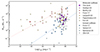 |
Fig. 9. Outflow rate vs. bolometric luminosity. The molecular outflow mass rates derived for the QSO2s using the three scenarios are displayed as large purple circles for the intermediate value, and dashed black lines connecting the most and least conservative values (small purple circles). For comparison, we included other molecular mass outflow rates measurements from the literature as circles of different colors: AGN and ULIRGs from Fiore et al. (2017), QSO2s from Girdhar et al. (2024), two type-1 QSOs from Fei et al. (2024), AGN-dominated ULIRGs from Lamperti et al. (2022), AGN with possibly jet-driven outflows from Papachristou et al. (2023), and the low-power jet-driven outflow from Murthy et al. (2022). Mass outflow rates reported for ionized outflows in the literature are shown with different symbols and shades of blue: AGN and ULIRGs from Fiore et al. (2017) as squares, local jetted-Seyfert galaxies from Venturi et al. (2021) as upward triangles, QSO2s at z < 0.4 from Ulivi et al. (2024) as downward triangles, and four of the QSO2s studied here from Speranza et al. (2024) as diamonds. The corresponding linear fits from Fiore et al. (2017) are shown as a salmon dot-dashed line for molecular outflows and as a blue dashed line for the ionized ones. The mass outflow rates from the literature have been converted to the thin shell geometry adopted in this work when necessary. |
We used three scenarios to compute the mass outflow rates, as described in Section 3.5, and found values of Ṁ = 5−150 M⊙ yr−1. The mass outflow rates that we derive from the most conservative scenario III if we exclude the radio-loud QSO2 J1347, are Ṁ = 5–16 M⊙ yr−1. These values are similar to those reported by RA22 using a different method, consisting of considering as outflowing gas that along the kinematic minor axis of the galaxies, and assuming that the outflows are coplanar with the CO disk. In Figure 9 we show the Ṁ versus Lbol plot including our QSO2s, with the intermediate values (big purple circles) representing scenario II and the black dashed lines connecting the least and most conservative values derived from scenarios I and III (small purple circles). In agreement with the results presented in RA22, our Ṁ values lie below the Fiore et al. (2017) empirical relation, even when we consider the least conservative scenario I. This is also the case for the AGN-dominated ULIRGs presented in Lamperti et al. (2022), also shown in Figure 9, whose outflow mass rates range from 3 to 145 M⊙ yr−1. Based on their bolometric luminosities (Lbol ∼ 1045 − 46 erg s−1), both our QSO2s and the AGN-dominated ULIRGs were expected to have molecular outflow rates of ≳100 M⊙ yr−1 based on the Fiore et al. (2017) scaling relation. The four z < 0.2 QSO2s with nuclear molecular outflows reported in Girdhar et al. (2024) also occupy the same region in the Ṁ−Lbol plane as the QSOFEED QSO2s.
This and other recent works are starting to reveal a population of AGN with less massive molecular outflows that those expected from empirical scaling relations. This is likely due to the advent of submillimeter facilities with high sensitivity such as ALMA and NOEMA, which enable the observation of more diverse, and hence less biased, AGN samples. Based on all the outflow measurements included in Figure 9, from this and other works, we claim that the scaling relations found by e.g. Cicone et al. (2014), Fiore et al. (2017), and Fluetsch et al. (2019) most likely represent the upper boundary of the Ṁ−LAGN relation, as first suggested by RA22.
We note that part of the discrepancy between the empirical Ṁ−LAGN relation and the observations lying below it in Figure 9 could be associated with the different outflow velocity definitions (e.g., vmax versus vout). For example, Venturi et al. (2023) reported that the use of vmax, defined as vout + FWHM/2, instead of vout results in an increase of the ionized mass outflow rates by a factor of 3–20. In the case of molecular outflows, which have lower velocities than the ionized ones, vout cannot be measured from the line wings in most cases, but rather from the residuals obtained after kinematical modeling, such as the analysis performed here. This is also the case of some of the molecular outflows used by Fiore et al. (2017) to derive the empirical relation shown in Figure 9, such as NGC 1068 (García-Burillo et al. 2014) and NGC 1433 (Combes et al. 2013). We refer the reader to Hervella Seoane et al. (2023) and Speranza et al. (2024) for further details on how the use of different methodologies and outflow parameter definitions affect the derived outflow energetics.
To explain these mild molecular outflows detected in luminous AGN, RA22 suggested that other factors including jet power, coupling between winds, jets, and/or ionized outflows and the CO disks, and the ISM distribution might also be relevant (see also Harrison & Ramos Almeida 2024 for a recent review). To investigate the possible role of compact jets as drivers of the molecular outflows, we computed the kinetic power of the outflows ( ) and compared them with the values of Lbol and the jet-power (Pjet) of the QSO2s and other AGN in Figure 10. The values of Pjet were computed using the 1.4 GHz VLA fluxes and spectral indices corresponding to the HR data from Jarvis et al. (2019) and applying the L1.4 GHz × Pjet relation of Bîrzan et al. (2008), as in AA23. They are listed in Table 4.
The observed kinetic powers of the QSO2 outflows are in the range of 6.4 × 1039 < Ėout < 1.2 × 1043 erg s−1, and in the left panel of Figure 10 we can see that the radiative coupling efficiencies, defined as  , lie below the 1:1000 relation, except for the least conservative value measured for J1347. This is showing that the kinetic power of the outflows correspond to ≪0.1% of the AGN bolometric luminosities shown in Table 1. There is a large scatter, of more than three orders of magnitude, in the ϵAGN derived when we considered the measurements from the three different scenarios (10−6 < ϵAGN < 10−4 if we only consider scenario II; 0.0001–0.01%). This scatter is similar to the one found for observationally derived outflow kinetic powers compiled by Harrison et al. (2018). Although the majority of the cosmological simulations require ϵAGN ≳ 1% for AGN feedback to efficiently suppress star formation (e.g. Dubois et al. 2014; Schaye et al. 2015; Costa et al. 2018), these fiducial efficiencies adopted in the simulations should not be directly compared to the observed coupling efficiencies (Costa et al. 2018; Harrison et al. 2018; Harrison & Ramos Almeida 2024). This is because theoretical efficiencies are calibrated quantities, and not a prediction from the simulations, and also because only a fraction of the injected energy is converted into outflow kinetic energy, depending on the properties of ISM, the gravitational potential, and other factors, so the observed coupling efficiencies are often small (Harrison & Ramos Almeida 2024).
Low radiative coupling efficiencies can also be due to the fact that radiation pressure–driven outflows depend strongly on the distribution and geometry of gas and dust around the AGN (Bieri et al. 2017; Costa et al. 2018). Radiative coupling efficiency depends on the degree to which radiation is trapped and reprocessed within an optically thick, dusty medium. In clumpy or porous environments, radiation can escape through low-density channels, significantly reducing the momentum imparted to the gas (e.g. Ishibashi & Fabian 2015; Costa et al. 2018). This strong dependence on the small-scale structure of the ISM can naturally explain the lower radiative coupling efficiencies observed in the quasars in this work. The purpose of showing Figure 10 including the 1:100 relation is to highlight that for the six QSO2s and for the majority of the observational data shown in that Figure, ϵAGN ≪ 1%.
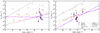 |
Fig. 10. Kinetic power of the outflow vs. bolometric luminosity (left panel) and jet power (right panel). The 1:1, 1:100, and 1:1000 relations are shown as dashed lines in both panels. The dashed purple line in both panels corresponds to the linear fit of the purple circles, which correspond to the molecular outflows of the QSO2s studied here (“QSOFEED mol.”). The diverging color line (“Quasars mol.”) represents the linear fit of the type-1 PG quasars in Fei et al. (2024, green circles), the QSO2s from Girdhar et al. (2024, magenta circles), and the QSOFEED QSO2s (purple circles). The light orange dot-dashed line (“All molecular”) shows the fit of all the molecular outflows mentioned before and those reported by Papachristou et al. (2023, yellow circles) and Murthy et al. (2022, red circles). Symbols and colors are the same as in Figure 9. |
For comparison, in the right panel of Figure 10 we present Ėout versus Pjet. The jet coupling efficiencies considering scenario II, defined as  , are in the range 0.001 < ϵjet < 0.035 (0.1–3.5%). These are similar to the jet coupling efficiencies of the four QSO2s at z < 0.2 reported by Girdhar et al. (2024), of 0.05–4% (one of them is Teacup, so in the following we will refer to the other three), and are significantly higher than the corresponding radiative coupling efficiencies.
We investigated possible correlations exiting between the outflow kinetic power, Ėout, and Lbol and Pjet. The first test was to apply a logarithmic linear regression to the six QSOFEED sources studied in this work. The second test was to group the six QSOFEED QSO2s and other nearby quasars with molecular outflows reported in the literature: three QSO2s at z ≲ 0.2 reported in Girdhar et al. (2024) and the two type-1 PG quasars at z ∼ 0.06 recently reported by Fei et al. (2024). Finally, the third test includes all the quasars included in the second test and the low-power jet-driven outflow in a low-luminosity AGN from Murthy et al. (2022) and the compilation of possibly jet-driven outflows in AGN of different bolometric luminosities presented in Papachristou et al. (2023).
In Table 5 we list the derived parameters for the logarithmic linear regression in the format log(Y) = a * log(X)+b, with the corresponding Pearson correlation coefficients, with possible values in the range of −1 < rPearson < 1 and the p-values. rPearson values close to zero indicate no correlation, close to 1 a strong correlation and close to −1 an anti-correlation.
Correlation parameters of the outflow energetics.
The p-values shown in Table 5 show that the only statistically significant correlations are found when considering all the measurements in the literature, i.e., the “All molecular” case, with p-value < 0.2% and rPearson ∼ 0.6, indicating a positive correlation with both Lbol and Pjet. On the other hand, when using the “QSOFEED molecular” (6 galaxies) and “Quasars molecular” (11 galaxies) samples, the p-values are high and indicate no correlations, possibly due to the small sample sizes. We note, however, that the linear regression using only the values of Ėout and Pjet derived for “QSOFEED molecular” (indicated with a purple dashed line in the right panel of Figure 10) follows the 1:1000 relation, indicating jet coupling efficiencies of ϵjet∼0.1%. This might indicate that the compact, low-power jets often detected in radio-quiet AGN, are potentially capable of launching the molecular outflows that we observe. To confirm or discard any of these trends, more observations covering larger parameter space in Pjet and Lbol are required.
Therefore, despite the fact that our QSO2s have high AGN luminosities, low-power jets might be driving some of the molecular outflows that we see, based on the higher jet coupling efficiencies reported here. This result is predicted by simulations of jet-ISM interactions (Mukherjee et al. 2018; Meenakshi et al. 2022) and in agreement with previous studies using similar samples of obscured quasars (e.g. Mullaney et al. 2013; Zakamska & Greene 2014; Jarvis et al. 2019; Molyneux et al. 2019; Girdhar et al. 2022, 2024). In fact, low-to-moderate power kiloparsec scale jets are starting to be recognized as potential drivers of multiphase outflows and as relevant mechanisms for AGN feedback (Morganti et al. 2015; Venturi et al. 2021). In radio-quiet quasars, spatially resolved radio structures are often associated with morphological and kinematic distinct features in the ionized and molecular gas, such as increased turbulence and outflowing bubbles (e.g. Villar-Martín et al. 2017; Jarvis et al. 2019, 2021; Girdhar et al. 2022; Ramos Almeida et al. 2022; Audibert et al. 2023; Ulivi et al. 2024). This suggest that jets can be an important feedback mechanism in highly accreting radio-quiet quasars, where radiative feedback would be expected to prevail. Alternatively, it has been proposed that the radio structures detected in e.g. VLA data of radio-quiet AGN could be produced by shocks induced by the outflows themselves as they made progress through the ambient ISM (Fischer et al. 2019, 2023).
We note that even if a jet-like morphology is resolved only for J1430 (Teacup) in the HR VLA radio images of our QSO2s, the unresolved radio emission of the others might still be attributed to small scale radio jets. Jarvis et al. (2019) analysed the VLA data of J1010, J1100, J13563, and J1430. They all show a radio excess and lie above the FIR–radio correlation of star-forming galaxies (Bell 2003), indicating that only star formation processes are not enough to produce their radio emission. In addition, Jarvis et al. (2019) classified the unresolved nuclear radio emission of these QSO2s as “jet/lobe/wind”, based on their steep spectral indices (α ∼ −0.8, see Table 4 in Jarvis et al. 2019). This hypothesis is confirmed for the case of J1347, which shows diffuse emission on large scales (r ∼ 80 kpc; Stanghellini et al. 2005) and an unresolved core using low angular resolution radio observations, but high angular resolution VLBI data revealed a 100 pc scale jet (Kellermann et al. 2004; Morganti et al. 2013), shown as black contours in the inset panel of J1347 in Figure 3.
The sensitivity and resolution of next generation radio facilities such as the LOw Frequency ARray (LOFAR), the Square Kilometre Array (SKA), and the new-generation Very Large Array (ngVLA) will help us to understand the origin of the radio emission in “radio-quiet” AGN (Panessa et al. 2019) and they likely will reveal a wealth of galactic scale jets (Nyland et al. 2018; Morabito et al. 2022; Ye et al. 2024). This will be particularly important to advance our understanding of the role of galactic scale low-power jets for AGN feedback, since “radio-quiet” sources dominate the AGN population (Padovani 2016).
4.2. Relative orientation of the multiphase outflows
In order to provide a more comprehensive view of the multiphase outflows detected in the quasars studied here, we compare our findings for the cold molecular gas (T ∼ 10–100 K) with observations in the optical and NIR, allowing us to probe a broad range of gas temperatures and densities (Cicone et al. 2018; Harrison & Ramos Almeida 2024). In the optical, the QSOFEED outflows have been studied in the warm ionized phase using the [O III]λ5007 Å emission line (T ∼ 104 K), and in the NIR using the ro-vibrational H2 lines to trace the warm molecular gas (T ≳ 103 K).
Using GTC/MEGARA integral field spectroscopic observations of five QSO2s (same as RA22 and this work, except for J1347), Speranza et al. (2024) characterized the morphology and kinematics of the [O III] emitting gas. According to the outflow properties there reported, the ionized outflows in these five QSO2s carry less mass than their molecular counterparts and are more extended (3.2 < rout < 12.6 kpc) and faster (500 < |vout|< 1300 km s−1) than the molecular outflows reported here (0.65 < rout < 2.4 kpc and 180 < |vout|< 300 km s−1 from scenario II). The orientations (PAs) of the ionized outflows are indicated in Figure 8 and Table 6 for comparison with the PAs measured here for the cold molecular outflows. The PA of J1010 could not be accurately measured from the GTC/MEGARA data, since this was the only QSO2 analyzed in Speranza et al. (2024) in which the [O III] outflow is not spatially resolved. From inspection of the kinematic maps shown by Speranza et al. (2024), however, the blueshifted side of the ionized outflow would have a PA of ∼ − 45°, i.e. towards the north-west. Ulivi et al. (2024) analyzed a VLT/MUSE cube of this QSO2 and also detected broad, blueshifted [OIII] emission, but without a clear outflow PA.
Position angles of the cold, warm molecular, and ionized outflows and radio jets.
We followed a similar procedure to that adopted in Speranza et al. (2024) to determine the PA of the blueshifted and/or redshifted sides of the molecular outflows. Speranza et al. (2024) fitted an ellipse to the 3σ contour of the O[III] outflow flux maps using a Python script (Hill 2016). Here we used the same script to fit ellipses to the global shape of the high-velocity contours in Figure 8. We then determined the outflow PA using the line connecting the QSO2 nucleus, defined by the 200 GHz continuum peak, and the most distant point within the ellipse. The cold molecular outflow PAs are listed in Table 6 and shown as dashed blue and red lines in Figure 8 for the blueshifted and redshifted sides of the outflows, respectively.
The projected PAs of the ionized and molecular outflows do not have similar orientations. In fact, in the cases of J1100, J1430, and J1509, their orientation appears to be inverted (see Figure 8). For instance, in J1430, the redshifted [O III] outflow (PA[OIII],red = 198°) is almost aligned with the blueshifted CO outflow (PACO, blue = 188°). The same is found for J1100 and J1509, where the redshifted sides of the CO outflows (PACO, red of 55° and −51°, respectively) are closely aligned with the blueshifted ionized outflow sides (PA[OIII],blue of 63° and −40°). A caveat to consider is that the MEGARA observations are seeing-limited, with a resolution of approximately 1 1, which is significantly coarser than the resolution of the ALMA data (∼0
 2), although in the case of well-resolved ionized outflows as is the case of J1100, J1356, J1430, and J1509 should not be an issue when it comes to determining the outflow orientation.
On the other hand, the warm molecular gas kinematics in J1356 and J1430, traced by the H21–0 S(1) and S(2) emission lines observed with VLT/SINFONI (seeing of ∼0 8), are consistent with that of the cold molecular gas observed by ALMA (Zanchettin et al. 2025). Both the blue- and redshifted sides of the warm molecular outflow are detected in J1430, while in J1356 only the redshifted outflow side is detected, having the same orientation observed for CO in this work (see Table 6), and similar radii and velocities (1.8 < rout < 1.9 kpc and 370 < |vout|< 470 km s−1). The main difference is that the warm molecular outflows represent just a small fraction of the total molecular gas mass: Zanchettin et al. (2025) measured warm-to-cold gas ratios of ∼1 × 10⁻⁵ in the two QSO2s (see Zanchettin et al. 2025, for further details on the comparison between cold and warm molecular gas in J1356 and J1430).
In general, the warm and cold molecular phases seem to be tracing the same outflow, with the main distinction being the mass fraction carried by them. On the contrary, the warm ionized outflows do not seem to be a different face of the same outflow, showing different orientation, velocity, and radius. This is likely related to the different temperatures and densities of the molecular and ionized gas, which respond differently to the action of AGN-driven winds and jets. This should be considered when comparing with simulations, which often consider “cold” gas that at temperatures of ∼103 − 104 K (e.g. Mukherjee et al. 2016; Ward et al. 2024).
4.3. Global versus localized physical conditions of the molecular gas
In Sections 3.2 and 3.3 we presented the R32 line ratios measured from the galaxy-integrated CO fluxes and the spatially resolved R32 maps of the QSO2s. The global values derived from the integrated CO(3–2) and CO(2–1) intensities listed in Table 3 are shown in the histogram of Figure 11. We compare our global R32 measurements with those derived for other samples of galaxies: a similar sample of 17 QSO2s at z < 0.2 from Molyneux et al. (2024) using either ACA or APEX CO integrated fluxes from J → 1 up to 7 transitions; 36 hard X-ray-selected AGN host galaxies from the BAT AGN Spectroscopic Survey (BASS) analyzed in Lamperti et al. (2020), observed with the 15 m single-dish James Clerk Maxwell Telescope; a sample of 36 local ULIRGs observed with APEX by Montoya Arroyave et al. (2023); and the low-J transitions study of a large sample of nearby star-forming disk galaxies using single-dish CO mapping surveys and PHANGS-ALMA by Leroy et al. (2022).
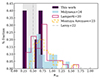 |
Fig. 11. Histogram of the integrated R32 for the five QSO2s for which CO(2–1) and CO(3–2) transitions are available. They are shown as filled purple bars. The values measured for a sample of QSO2s at z < 0.2 from Molyneux et al. (2024) are also shown in light blue, for the X-ray selected AGN reported by Lamperti et al. (2020) in pink, of the local ULIRGs presented in Montoya Arroyave et al. (2023) in yellow, and the mean value measured for star-forming disk galaxies from Leroy et al. (2022) is the gray dot-dashed line, with the corresponding interval shown as a shaded gray area. |
We derived integrated values of 0.22 < R32 < 0.75 and an average value of ⟨R32⟩0.5 ± 0.2 for the QSO2s, which is similar to the average values derived for normal disk galaxies in Leroy et al. (2022), of 0.23 < R32 < 0.59. Molyneux et al. (2024) reported a median value of ⟨R32⟩ = 0.6 for their sample of QSO2s, similar to ours, but their values range from 0.37 to 1.46, a broader range than the one we found for our smaller sample. A slightly higher average value of ⟨R32⟩> 0.74 ± 0.3 was measured for the AGN BASS sample by Lamperti et al. (2020), with ratios ranging from 0.3 to 1.7. A similarly broad interval of R32 was found by Montoya Arroyave et al. (2023) for a sample of ULIRGs including active and non-active galaxies, with a median value of ⟨R32⟩ = 0.76 and a range of 0.4 < R32 < 1.7.
The CO SLEDs derived for QSO2s at z < 0.2 by Molyneux et al. (2024) do not show evidence for a high gas excitation for high J → 6,7 transitions, as was observed for more luminous high-redshift quasars (Carilli & Walter 2013). We note, however, that only one of the four QSO2s observed in CO(6–5) by Molyneux et al. (2024) was detected, and none of the three QSO2s observed in CO(7–6) was detected. These authors concluded that AGN feedback is not exerting any influence in the overall gas excitation on global scales, and instead, they proposed that feedback from winds/jets might by occurring on localized regions that they cannot resolve with the ACA/APEX observations. For lower J transitions, the CO SLEDs of a sample of 35 local AGN (z ≤ 0.15) reported by Esposito et al. (2022) indicate no evidence for AGN influence on the cold and low-density gas on more localized kiloparsec-scales.
The high angular resolution ALMA observations employed here allow us to probe physical scales of a few hundreds of parsecs of the QSO2s. The spatially resolved R32 maps shown in Figure 3 reveal a gradient of excitation, with higher values of R32 ∼ 0.7–0.9 within the central kiloparsec of the galaxies and of ∼0.2–0.5 across the galaxy disks. Spatially resolved CO line ratio emission analyses have been reported for a few nearby Seyferts and radio galaxies (Viti et al. 2014; Morganti et al. 2015; Dasyra et al. 2016; Oosterloo et al. 2017, 2019; Ruffa et al. 2022), but not for quasars, with the exception of the Teacup (AA23).
Using a plethora of molecular lines (i.e., CO, HCN, HCO+, and CS lines) and the RADEX (van der Tak et al. 2007) radiative transfer code, Viti et al. (2014) modeled the excitation conditions of the molecular gas in the circumnuclear disk of NGC 1068. The authors claimed that elevated values of R31 ≡ L′CO(3 − 2)/L′CO(1 − 0) ∼ 5 and R21 ≡ L′CO(2 − 1)/L′CO(1 − 0) ≳ 4 correspond to hot dense gas (kinetic temperatures T > 150 K and gas density nH > 105 cm−3) excited by the AGN.
Higher values of different emission line ratios have been reported for the molecular gas interacting with jets in the radio galaxy PKS 1549-79 (Oosterloo et al. 2019), and also in the Seyfert galaxy IC 5063 (Dasyra et al. 2016; Oosterloo et al. 2017). IC 5063 is a clear-cut example of jet coplanar with the galaxy disk, which is driving a multiphase outflow (Tadhunter et al. 2014; Morganti et al. 2015). The jet power estimated for IC 5063 is Pjet ∼ 1044 erg s−1 and the PVD along the jet axis revealed R32 values ranging from 1.0−1.5 in the outflowing regions, clearly different from the gas following regular rotation (R32 < 0.7). Under local thermodynamic equilibrium (LTE) conditions, R32 > 1 corresponds to excitation temperatures (Tex) of ∼50 K (Oosterloo et al. 2017). A similar temperature was found for the fast outflow gas component of IC 5063 using R42 ≡ L′CO(4 − 3)/L′CO(2 − 1) ≫ 1, suggesting that the gas in the outflow is optically thin (Dasyra et al. 2016).
Another example of jet-induced molecular gas excitation is the radio galaxy NGC 3100. The cold molecular gas is distributed in a ring-like morphology, with the central region (∼500 pc) depleted of CO. Most of the CO emission presents R21 and R31 ratios of < 1, implying subthermal excitation conditions (Ruffa et al. 2022), but ratios of R21 ∼ 4 and R31 ∼ 3 are observed at the inner part of the disk, where there is spatial correlation with the radio lobes. All these cases indicate that jet-impacted regions have different gas excitation conditions due to shocks and/or reduced optical thickness (Morganti et al. 2021).
In an attempt to quantify the differences in R32 found between the disk and outflow regions, Figure 12 shows the histograms of R32 values included in the PVDs along the minor axis (see Figures 4–7). The green histograms correspond to molecular gas with velocities v < vout from scenario II, which we attributed to the disk, and the red histograms to gas with v > vout, which we associate with the outflow regions. We note that this method only includes gas along the minor axis, within a simulated slit of a given size, and therefore does not include all the gas in the disk or outflow. The outflow histograms show higher values of R32 than the disk ones in J1100, J1347, and J1356. In the case of J1010, as we described in Section 3.4, the regions with R32 > 1 are distributed all over the minor and major axis PVDs, for both low and high velocity gas. This is likely related to coarser resolution of the CO(2–1) data in the case of J1010, of ∼0 8, which prevents us from accurately constraining the R32 distribution in this QSO2. For J1430, studied in detail in AA23, the jet is almost coplanar with the CO disk, producing elevated R32 values across the whole disk, and particularly along the direction perpendicular to the jet.
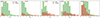 |
Fig. 12. Distribution of the R32 values in the PVD along the minor axis for the high-velocity (red) and disk regions (green) shown in Figures 4–7. |
Therefore, based on the analysis presented in this work, for our QSO2s we find that the regions with high-velocity gas that cannot be attributed to rotation, as modeled with 3DBAROLO, have values of R32 of up to ≈1–2, with J1347 showing the highest values. These values are significantly higher than those measured in areas of the PVDs dominated by rotation (R32 ≈ 0.3–0.7) and than the values reported by Leroy et al. (2022) for normal disk galaxies (mean R32 of 0.5), indicating that the molecular gas participating in the outflows exhibits enhanced temperature and is optically thin. Shocks could potentially induce a different temperature profile and thus affect the observed line ratios in these outflows (Meijerink et al. 2013). This could also be due to higher X-ray emission in the vicinity of the AGN, since R32 tends to increase with the X-ray luminosity in high density gas (nH > 104 cm−3), as shown in Lamperti et al. (2020). We are unable to infer the physical conditions (Tex and density) of the gas using only one molecular line ratio, however, because more transitions, especially from higher J, would be necessary for that.
5. Conclusions
We presented the analysis of ALMA CO(2–1) and CO(3–2) observations at 0 2–0
2–0 6 resolution (370–960 pc) of a sample of six obscured quasars at z ∼ 0.1, which belong to the QSOFEED sample. Our goal was to investigate the relevance of quasar-driven winds and/or jets on their cold molecular ISM and kinematics. To do this, we performed a kinematic modeling together with spatially resolved line ratios, R32, which indicated changes in the gas excitation conditions. Our main findings are summarized below.
– The CO(3–2) emission of the QSO2s, even when it is measured from data with a slightly lower angular resolution (0 6), shows a similar morphology and kinematics than those of the CO(2–1) emission that were first presented by RA22. The peak-intensity maps reveal clumpy structures and double-peaked morphologies better than the corresponding moment-0 maps.
– The line ratios using the integrated CO(2–1) and CO(3–2) fluxes measured for our sample range from 0.22 < R32 < 0.75, with an average value of ⟨R32⟩ = 0.5 ± 0.2. This is similar to the line ratios that are typically found in the galaxy disks of nearby star-forming galaxies. In principle, this implies no impact of the AGN on the global molecular gas excitation. Our spatially resolved R32 maps reveal an excitation gradient, however, with higher values of R32 ∼ 0.7–0.9 within the central kiloparsec of the galaxies that decrease to values of ∼0.2–0.5 across the galaxy disks. The regions in which the excitation is higher coincide with areas in which the velocity dispersion is high, but we found no clear trend between the orientation of this enhancement of the gas excitation and the dispersion either along or perpendicular to the radio emission, with the exception of the Teacup (J1430), as previously reported by AA23.
– The combination of kinematic modeling with 3DBAROLO and the R32 PVDs revealed that the high-velocity regions associated with outflows have the highest line ratios seen in the PVD. They exceed R32 > 1. This indicates that either the high-velocity gas presents a higher gas excitation (higher temperatures) or that it is optically thin.
– Using three scenarios to compute the mass outflow rates, we found values ranging from Ṁ = 5−150 M⊙ yr−1. These values lie below the Ṁ−Lbol empirical relations reported in the literature (e.g., Fiore et al. 2017), even when we considered the least conservative scenario I.
– We measured outflow kinetic powers in the range of 6.4 × 1039 < Ėout < 1.2 × 1043 erg s−1 for our QSO2s. The radiative coupling efficiencies ( ) ranged from 10−6 < ϵAGN < 10−4 when we used the kinetic powers derived from scenario II, corresponding to coupling efficiencies of ≪0.1%. On the other hand, the jet coupling efficiencies (
 ) ranged from 0.001 < ϵjet < 0.035 (ϵjet ∼ 0.1%). These findings might indicate that, despite the high AGN luminosities of the QSO2s (Lbol ∼ 1045.5 − 46 erg s−1), compact low-power jets might be playing a key role in driving the molecular outflows.
– By comparing the cold molecular outflow properties with those derived for some of the QSO2s in the ionized (Speranza et al. 2024) and warm molecular gas phases (Zanchettin et al. 2025), we found that the warm and cold molecular phases appear to be tracing the same outflow, while the warm ionized phases does not, as it exhibits distinct orientation and kinematics.
To better understand the role of jets and winds on the distribution, kinematics, and gas excitation of molecular gas in radio-quiet quasars, CO and radio observations with a high angular resolution of larger samples are required. In particular, data with a high angular resolution of multiple CO transitions will be crucial to distinguish the outflow from regular kinematics, to characterize the impact of winds and jets on gas with different molecular gas densities, and to constrain the excitation mechanisms.
We note that the double-peaked morphologies seen in CO do not mean the galaxy necessarily host two nuclei. For the cases in which there are two nuclei identified in the optical images and in ALMA continuum at 200 GHz, namely J1347 and J1356, we show the position of the second nucleus in Figure 2 as blue stars.


Acknowledgments
The authors acknowledge the anonymous referee for their constructive report. AA and CRA acknowledge support from the Agencia Estatal de Investigación of the Ministerio de Ciencia, Innovación y Universidades (MCIU/AEI) under the grant “Tracking active galactic nuclei feedback from parsec to kiloparsec scales”, with reference PID2022−141105NB−I00 and the European Regional Development Fund (ERDF). They also acknowledge the projects “Quantifying the impact of quasar feedback on galaxy evolution”, with reference EUR2020-112266, funded by MICINN-AEI/10.13039/501100011033 and the European Union NextGenerationEU/PRTR, and the Consejería de Economía, Conocimiento y Empleo del Gobierno de Canarias and the European Regional Development Fund (ERDF) under grant “Quasar feedback and molecular gas reservoirs”, with reference ProID2020010105, ACCISI/FEDER, UE. AA acknowledges funding from the MICINN (Spain) through the Juan de la Cierva-Formación program under contract FJC2020-046224-I and from the European Union grant WIDERA ExGal-Twin, GA 101158446. SGB acknowledges support from the Spanish grant PID2022-138560NB-I00, funded by MCIN/AEI/10.13039/501100011033/FEDER, EU. MPS acknowledges support under grants RYC2021-033094-I, CNS2023-145506, and PID2023-146667NB-I00 funded by MCIN/AEI/10.13039/501100011033 and the European Union NextGenerationEU/PRTR. IL acknowledges support from PRIN-MUR project “PROMETEUS” (202223XPZM). This paper makes use of the following ALMA data: ADS/JAO.ALMA#2018.1.00870.S, ADS/JAO.ALMA#2016.1.01535.S, ADS/JAO.ALMA#2018.1.01767.S, ADS/JAO.ALMA#2018.1.00699.S, ADS/JAO.ALMA#2013.1.00180.S, ADS/JAO.ALMA#2011.0.00652.S, ADS/JAO.ALMA#2012.1.00797.S, and ADS/JAO.ALMA#2016.1.01535.S. ALMA is a partnership of ESO (representing its member states), NSF (USA) and NINS (Japan), together with NRC(Canada) and NSC and ASIAA (Taiwan), in cooperation with the Republic of Chile. The Joint ALMA Observatory is operated by ESO, AUI/NRAO and NAOJ. The National Radio Astronomy Observatory is a facility of the National Science Foundation operated under cooperative agreement by Associated Universities, Inc.
References
- Audibert, A., Combes, F., García-Burillo, S., et al. 2019, A&A, 632, A33 [NASA ADS] [CrossRef] [EDP Sciences] [Google Scholar]
- Audibert, A., Combes, F., García-Burillo, S., et al. 2021, A&A, 656, A60 [NASA ADS] [CrossRef] [EDP Sciences] [Google Scholar]
- Audibert, A., Ramos Almeida, C., García-Burillo, S., et al. 2023, A&A, 671, L12 [NASA ADS] [CrossRef] [EDP Sciences] [Google Scholar]
- Becker, R. H., White, R. L., & Helfand, D. J. 1995, ApJ, 450, 559 [Google Scholar]
- Bell, E. F. 2003, ApJ, 586, 794 [Google Scholar]
- Bessiere, P. S., Ramos Almeida, C., Holden, L. R., Tadhunter, C. N., & Canalizo, G. 2024, A&A, 689, A271 [NASA ADS] [CrossRef] [EDP Sciences] [Google Scholar]
- Bieri, R., Dubois, Y., Rosdahl, J., et al. 2017, MNRAS, 464, 1854 [NASA ADS] [CrossRef] [Google Scholar]
- Bîrzan, L., McNamara, B. R., Nulsen, P. E. J., Carilli, C. L., & Wise, M. W. 2008, ApJ, 686, 859 [Google Scholar]
- Bolatto, A. D., Wolfire, M., & Leroy, A. K. 2013, ARA&A, 51, 207 [CrossRef] [Google Scholar]
- Bournaud, F., Duc, P. A., & Emsellem, E. 2008, MNRAS, 389, L8 [NASA ADS] [CrossRef] [Google Scholar]
- Bournaud, F., Powell, L. C., Chapon, D., & Teyssier, R. 2011, in Astrophysical Dynamics: From Stars to Galaxies, eds. N. H. Brummell, A. S. Brun, M. S. Miesch, & Y. Ponty, 271, 160 [Google Scholar]
- Bourne, M. A., & Sijacki, D. 2017, MNRAS, 472, 4707 [NASA ADS] [CrossRef] [Google Scholar]
- Bourne, M. A., & Yang, H.-Y. K. 2023, Galaxies, 11, 73 [NASA ADS] [CrossRef] [Google Scholar]
- Carilli, C. L., & Walter, F. 2013, ARA&A, 51, 105 [NASA ADS] [CrossRef] [Google Scholar]
- Cicone, C., Maiolino, R., Sturm, E., et al. 2014, A&A, 562, A21 [NASA ADS] [CrossRef] [EDP Sciences] [Google Scholar]
- Cicone, C., Brusa, M., Ramos Almeida, C., et al. 2018, Nat. Astron., 2, 176 [Google Scholar]
- Combes, F., García-Burillo, S., Casasola, V., et al. 2013, A&A, 558, A124 [NASA ADS] [CrossRef] [EDP Sciences] [Google Scholar]
- Costa, T., Rosdahl, J., Sijacki, D., & Haehnelt, M. G. 2018, MNRAS, 473, 4197 [Google Scholar]
- Croton, D. J., Springel, V., White, S. D. M., et al. 2006, MNRAS, 365, 11 [Google Scholar]
- Dasyra, K. M., Combes, F., Oosterloo, T., et al. 2016, A&A, 595, L7 [NASA ADS] [CrossRef] [EDP Sciences] [Google Scholar]
- Di Matteo, T., Colberg, J., Springel, V., Hernquist, L., & Sijacki, D. 2008, ApJ, 676, 33 [NASA ADS] [CrossRef] [Google Scholar]
- Di Teodoro, E. M., & Fraternali, F. 2015, MNRAS, 451, 3021 [Google Scholar]
- Downes, D., & Solomon, P. M. 1998, ApJ, 507, 615 [NASA ADS] [CrossRef] [Google Scholar]
- Dubois, Y., Pichon, C., Welker, C., et al. 2014, MNRAS, 444, 1453 [Google Scholar]
- Dubois, Y., Peirani, S., Pichon, C., et al. 2016, MNRAS, 463, 3948 [Google Scholar]
- Esposito, F., Vallini, L., Pozzi, F., et al. 2022, MNRAS, 512, 686 [NASA ADS] [CrossRef] [Google Scholar]
- Esposito, F., Vallini, L., Pozzi, F., et al. 2024, MNRAS, 527, 8727 [Google Scholar]
- Fabian, A. C. 2012, ARA&A, 50, 455 [Google Scholar]
- Fei, Q., Wang, R., Molina, J., et al. 2024, ApJ, accepted [arXiv:2409.15611] [Google Scholar]
- Feruglio, C., Maiolino, R., Piconcelli, E., et al. 2010, A&A, 518, L155 [NASA ADS] [CrossRef] [EDP Sciences] [Google Scholar]
- Feruglio, C., Fabbiano, G., Bischetti, M., et al. 2020, ApJ, 890, 29 [Google Scholar]
- Fiore, F., Feruglio, C., Shankar, F., et al. 2017, A&A, 601, A143 [NASA ADS] [CrossRef] [EDP Sciences] [Google Scholar]
- Fischer, T., Smith, K. L., Kraemer, S., et al. 2019, ApJ, 887, 200 [Google Scholar]
- Fischer, T. C., Johnson, M. C., Secrest, N. J., Crenshaw, D. M., & Kraemer, S. B. 2023, ApJ, 953, 87 [NASA ADS] [CrossRef] [Google Scholar]
- Fluetsch, A., Maiolino, R., Carniani, S., et al. 2019, MNRAS, 483, 4586 [NASA ADS] [Google Scholar]
- Fotopoulou, C. M., Dasyra, K. M., Combes, F., Salomé, P., & Papachristou, M. 2019, A&A, 629, A30 [NASA ADS] [CrossRef] [EDP Sciences] [Google Scholar]
- García-Burillo, S., Combes, F., Usero, A., et al. 2014, A&A, 567, A125 [Google Scholar]
- García-Burillo, S., Combes, F., Usero, A., et al. 2015, A&A, 580, A35 [Google Scholar]
- García-Burillo, S., Combes, F., Ramos Almeida, C., et al. 2019, A&A, 632, A61 [Google Scholar]
- García-Burillo, S., Alonso-Herrero, A., Ramos Almeida, C., et al. 2021, A&A, 652, A98 [NASA ADS] [CrossRef] [Google Scholar]
- García-Burillo, S., Hicks, E. K. S., Alonso-Herrero, A., et al. 2024, A&A, 689, A347 [NASA ADS] [CrossRef] [EDP Sciences] [Google Scholar]
- Girdhar, A., Harrison, C. M., Mainieri, V., et al. 2022, MNRAS, 512, 1608 [NASA ADS] [CrossRef] [Google Scholar]
- Girdhar, A., Harrison, C. M., Mainieri, V., et al. 2024, MNRAS, 527, 9322 [Google Scholar]
- Harrison, C. M. 2017, Nat. Astron., 1, 0165 [NASA ADS] [CrossRef] [Google Scholar]
- Harrison, C. M., Costa, T., Tadhunter, C. N., et al. 2018, Nat. Astron., 2, 198 [Google Scholar]
- Harrison, C. M., & Ramos Almeida, C. 2024, Galaxies, 12, 17 [NASA ADS] [CrossRef] [Google Scholar]
- Hervella Seoane, K., Ramos Almeida, C., Acosta-Pulido, J. A., et al. 2023, A&A, 680, A71 [NASA ADS] [CrossRef] [EDP Sciences] [Google Scholar]
- Hickox, R. C., Mullaney, J. R., Alexander, D. M., et al. 2014, ApJ, 782, 9 [NASA ADS] [CrossRef] [Google Scholar]
- Hill, C. 2016, Learning Scientific Programming with Python (Cambridge: Cambridge University Press) [Google Scholar]
- Holden, L. R., Tadhunter, C., Audibert, A., et al. 2024, MNRAS, 530, 446 [NASA ADS] [CrossRef] [Google Scholar]
- Hollenbach, D. J., & Tielens, A. G. G. M. 1999, Rev. Mod. Phys., 71, 173 [Google Scholar]
- Ishibashi, W., & Fabian, A. C. 2015, MNRAS, 451, 93 [NASA ADS] [CrossRef] [Google Scholar]
- Jarvis, M. E., Harrison, C. M., Thomson, A. P., et al. 2019, MNRAS, 485, 2710 [Google Scholar]
- Jarvis, M. E., Harrison, C. M., Mainieri, V., et al. 2021, MNRAS, 503, 1780 [NASA ADS] [CrossRef] [Google Scholar]
- Kellermann, K. I., Lister, M. L., Homan, D. C., et al. 2004, ApJ, 609, 539 [NASA ADS] [CrossRef] [Google Scholar]
- King, A. 2003, ApJ, 596, L27 [Google Scholar]
- King, A., & Nixon, C. 2015, MNRAS, 453, L46 [NASA ADS] [CrossRef] [Google Scholar]
- Kong, M., & Ho, L. C. 2018, ApJ, 859, 116 [NASA ADS] [CrossRef] [Google Scholar]
- Lamastra, A., Bianchi, S., Matt, G., et al. 2009, A&A, 504, 73 [NASA ADS] [CrossRef] [EDP Sciences] [Google Scholar]
- Lamperti, I., Saintonge, A., Koss, M., et al. 2020, ApJ, 889, 103 [Google Scholar]
- Lamperti, I., Pereira-Santaella, M., Perna, M., et al. 2022, A&A, 668, A45 [NASA ADS] [CrossRef] [EDP Sciences] [Google Scholar]
- Leroy, A. K., Rosolowsky, E., Usero, A., et al. 2022, ApJ, 927, 149 [NASA ADS] [CrossRef] [Google Scholar]
- Lutz, D., Sturm, E., Janssen, A., et al. 2020, A&A, 633, A134 [NASA ADS] [CrossRef] [EDP Sciences] [Google Scholar]
- Mandal, A., Mukherjee, D., Federrath, C., et al. 2021, MNRAS, 508, 4738 [NASA ADS] [CrossRef] [Google Scholar]
- Martini, P. 2004, ASP Conf. Ser., 376, 127 [Google Scholar]
- McNamara, B. R., & Nulsen, P. E. J. 2012, New J. Phys., 14, 055023 [NASA ADS] [CrossRef] [Google Scholar]
- Meenakshi, M., Mukherjee, D., Wagner, A. Y., et al. 2022, MNRAS, submitted [arXiv:2203.10251] [Google Scholar]
- Meijerink, R., Spaans, M., & Israel, F. P. 2007, A&A, 461, 793 [NASA ADS] [CrossRef] [EDP Sciences] [Google Scholar]
- Meijerink, R., Kristensen, L. E., Weiß, A., et al. 2013, ApJ, 762, L16 [Google Scholar]
- Mingozzi, M., Vallini, L., Pozzi, F., et al. 2018, MNRAS, 474, 3640 [NASA ADS] [CrossRef] [Google Scholar]
- Molyneux, S. J., Harrison, C. M., & Jarvis, M. E. 2019, A&A, 631, A132 [NASA ADS] [CrossRef] [EDP Sciences] [Google Scholar]
- Molyneux, S. J., Calistro Rivera, G., De Breuck, C., et al. 2024, MNRAS, 527, 4420 [Google Scholar]
- Montoya Arroyave, I., Cicone, C., Makroleivaditi, E., et al. 2023, A&A, 673, A13 [NASA ADS] [CrossRef] [EDP Sciences] [Google Scholar]
- Morabito, L. K., Jackson, N. J., Mooney, S., et al. 2022, A&A, 658, A1 [NASA ADS] [CrossRef] [EDP Sciences] [Google Scholar]
- Morganti, R., Fogasy, J., Paragi, Z., Oosterloo, T., & Orienti, M. 2013, Science, 341, 1082 [NASA ADS] [CrossRef] [Google Scholar]
- Morganti, R., Oosterloo, T., Oonk, J. B. R., Frieswijk, W., & Tadhunter, C. 2015, A&A, 580, A1 [NASA ADS] [CrossRef] [EDP Sciences] [Google Scholar]
- Morganti, R., Oosterloo, T., Murthy, S., & Tadhunter, C. 2021, Astron. Nachr., 342, 1135 [NASA ADS] [CrossRef] [Google Scholar]
- Mukherjee, D., Bicknell, G. V., Sutherland, R., & Wagner, A. 2016, MNRAS, 461, 967 [NASA ADS] [CrossRef] [Google Scholar]
- Mukherjee, D., Bicknell, G. V., Wagner, A. Y., Sutherland, R. S., & Silk, J. 2018, MNRAS, 479, 5544 [NASA ADS] [CrossRef] [Google Scholar]
- Mullaney, J. R., Alexander, D. M., Fine, S., et al. 2013, MNRAS, 433, 622 [Google Scholar]
- Murthy, S., Morganti, R., Wagner, A. Y., et al. 2022, Nat. Astron., 6, 488 [CrossRef] [Google Scholar]
- Nelson, D., Pillepich, A., Springel, V., et al. 2019, MNRAS, 490, 3234 [Google Scholar]
- Nyland, K., Harwood, J. J., Mukherjee, D., et al. 2018, ApJ, 859, 23 [NASA ADS] [CrossRef] [Google Scholar]
- Oosterloo, T., Raymond Oonk, J. B., Morganti, R., et al. 2017, A&A, 608, A38 [NASA ADS] [CrossRef] [EDP Sciences] [Google Scholar]
- Oosterloo, T., Morganti, R., Tadhunter, C., et al. 2019, A&A, 632, A66 [NASA ADS] [CrossRef] [EDP Sciences] [Google Scholar]
- Padovani, P. 2016, A&ARv, 24, 13 [Google Scholar]
- Panessa, F., Baldi, R. D., Laor, A., et al. 2019, Nat. Astron., 3, 387 [Google Scholar]
- Papachristou, M., Dasyra, K. M., Fernández-Ontiveros, J. A., et al. 2023, A&A, 679, A115 [NASA ADS] [CrossRef] [EDP Sciences] [Google Scholar]
- Pereira-Santaella, M., Colina, L., García-Burillo, S., et al. 2018, A&A, 616, A171 [NASA ADS] [CrossRef] [EDP Sciences] [Google Scholar]
- Pierce, J. C. S., Tadhunter, C., Ramos Almeida, C., et al. 2023, MNRAS, 522, 1736 [NASA ADS] [CrossRef] [Google Scholar]
- Ramos Almeida, C., Piqueras López, J., Villar-Martín, M., & Bessiere, P. S. 2017, MNRAS, 470, 964 [NASA ADS] [CrossRef] [Google Scholar]
- Ramos Almeida, C., Acosta-Pulido, J. A., Tadhunter, C. N., et al. 2019, MNRAS, 487, L18 [NASA ADS] [CrossRef] [Google Scholar]
- Ramos Almeida, C., Bischetti, M., García-Burillo, S., et al. 2022, A&A, 658, A155 [NASA ADS] [CrossRef] [EDP Sciences] [Google Scholar]
- Ramos Almeida, C., García-Bernete, I., Pereira-Santaella, M., et al. 2025, A&A, 698, A194 [NASA ADS] [CrossRef] [EDP Sciences] [Google Scholar]
- Reyes, R., Zakamska, N. L., Strauss, M. A., et al. 2008, AJ, 136, 2373 [Google Scholar]
- Ruffa, I., Prandoni, I., Davis, T. A., et al. 2022, MNRAS, 510, 4485 [NASA ADS] [CrossRef] [Google Scholar]
- Rupke, D. S., Veilleux, S., & Sanders, D. B. 2005, ApJS, 160, 115 [Google Scholar]
- Schawinski, K., Koss, M., Berney, S., & Sartori, L. F. 2015, MNRAS, 451, 2517 [Google Scholar]
- Schaye, J., Crain, R. A., Bower, R. G., et al. 2015, MNRAS, 446, 521 [Google Scholar]
- Solomon, P. M., & Vanden Bout, P. A. 2005, ARA&A, 43, 677 [NASA ADS] [CrossRef] [Google Scholar]
- Speranza, G., Ramos Almeida, C., Acosta-Pulido, J. A., et al. 2022, A&A, 665, A55 [NASA ADS] [CrossRef] [EDP Sciences] [Google Scholar]
- Speranza, G., Ramos Almeida, C., Acosta-Pulido, J. A., et al. 2024, A&A, 681, A63 [NASA ADS] [CrossRef] [EDP Sciences] [Google Scholar]
- Stanghellini, C., O’Dea, C. P., Dallacasa, D., et al. 2005, A&A, 443, 891 [NASA ADS] [CrossRef] [EDP Sciences] [Google Scholar]
- Sun, A.-L., Greene, J. E., Zakamska, N. L., & Nesvadba, N. P. H. 2014, ApJ, 790, 160 [NASA ADS] [CrossRef] [Google Scholar]
- Tacconi, L. J., Neri, R., Genzel, R., et al. 2013, ApJ, 768, 74 [NASA ADS] [CrossRef] [Google Scholar]
- Tadhunter, C., Morganti, R., Rose, M., Oonk, J. B. R., & Oosterloo, T. 2014, Nature, 511, 440 [Google Scholar]
- Talbot, R. Y., Sijacki, D., & Bourne, M. A. 2022, MNRAS, 514, 4535 [NASA ADS] [CrossRef] [Google Scholar]
- Ulivi, L., Venturi, G., Cresci, G., et al. 2024, A&A, 685, A122 [NASA ADS] [CrossRef] [EDP Sciences] [Google Scholar]
- Valentini, M., Murante, G., Borgani, S., et al. 2020, MNRAS, 491, 2779 [Google Scholar]
- Vallini, L., Tielens, A. G. G. M., Pallottini, A., et al. 2019, MNRAS, 490, 4502 [CrossRef] [Google Scholar]
- van der Tak, F. F. S., Black, J. H., Schöier, F. L., Jansen, D. J., & van Dishoeck, E. F. 2007, A&A, 468, 627 [NASA ADS] [CrossRef] [EDP Sciences] [Google Scholar]
- van der Werf, P. P., Isaak, K. G., Meijerink, R., et al. 2010, A&A, 518, L42 [NASA ADS] [CrossRef] [EDP Sciences] [Google Scholar]
- Veilleux, S., Maiolino, R., Bolatto, A. D., & Aalto, S. 2020, A&ARv, 28, 2 [NASA ADS] [CrossRef] [Google Scholar]
- Venturi, G., Cresci, G., Marconi, A., et al. 2021, A&A, 648, A17 [NASA ADS] [CrossRef] [EDP Sciences] [Google Scholar]
- Venturi, G., Treister, E., Finlez, C., et al. 2023, A&A, 678, A127 [NASA ADS] [CrossRef] [EDP Sciences] [Google Scholar]
- Villar-Martín, M., Emonts, B., Cabrera Lavers, A., et al. 2017, MNRAS, 472, 4659 [Google Scholar]
- Viti, S., García-Burillo, S., Fuente, A., et al. 2014, A&A, 570, A28 [NASA ADS] [CrossRef] [EDP Sciences] [Google Scholar]
- Ward, S. R., Costa, T., Harrison, C. M., & Mainieri, V. 2024, MNRAS, 533, 1733 [Google Scholar]
- Whitmore, B. C., Brogan, C., Chandar, R., et al. 2014, ApJ, 795, 156 [NASA ADS] [CrossRef] [Google Scholar]
- Ye, H., Sweijen, F., van Weeren, R. J., et al. 2024, A&A, 691, A347 [NASA ADS] [CrossRef] [EDP Sciences] [Google Scholar]
- Zakamska, N. L., & Greene, J. E. 2014, MNRAS, 442, 784 [Google Scholar]
- Zanchettin, M. V., Feruglio, C., Bischetti, M., et al. 2021, A&A, 655, A25 [NASA ADS] [CrossRef] [EDP Sciences] [Google Scholar]
- Zanchettin, M. V., Ramos Almeida, C., Audibert, A., et al. 2025, A&A, 695, A185 [NASA ADS] [CrossRef] [EDP Sciences] [Google Scholar]
- Zubovas, K., & King, A. 2012, ApJ, 745, L34 [Google Scholar]
Appendix A: Radio observations
We describe the main properties of the radio continuum observations used in this work. In Table A.1 we list the telescope and observed frequency, the synthesized beam size, rms and project name. We note that in the case of VLA observations, we only report the values for the HR configuration from Jarvis et al. (2019), which were the mostly used in this work.
Properties of the radio observations.
Appendix B: 3DBAROLO modeling
The results of the kinematic modeling using 3DBAROLO are shown in Figures B.1-B.5 for the CO(3–2) emission. The main parameters derived from the best fit of the CO(3–2) data and of the CO(2–1) datacubes degraded to the resolution of CO(3–2) are shown in Table B.1. All parameters are in agreement with the values obtained from the kinematic modeling presented in RA22.
3DBAROLO best fits for the CO(2–1) and CO(3–2) data.
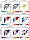 |
Fig. B.1. 3DBAROLO kinematic maps of the CO(3–2) emission of J1010. The panels on the left show the data, the middle panels show the best 3DBAROLO model, and the residuals (data-model) are shown on the right panels for the intensity (top row), velocity field (middle row), and velocity dispersion (bottom row). The cross represents the continuum peak at 200 GHz, and the PA of the kinematic major axis of the galaxy is indicated with dashed lines. |
Appendix C: Dispersion and rotation dominated systems
We present the velocity over the velocity dispersion maps, v/σ, for the six QSO2s studied in this work in Figure C.1. To create the v/σ maps we used the higher resolution CO(2–1) observations, except for J1010, for which we used the higher spatial resolution CO(3–2) data.
All but one systems appear to be rotation-dominated in most of the emitting regions according to the criterion v/σ> 1, highlighted by the dotted blue lines showing the v/σ = 1 contour. The regions showing v/σ< 1 correspond to the line of zeros in the velocity field, as expected for rotation along the minor axis of the galaxies. The exception is J1356, where high velocity dispersion values (v/σ< 1) dominate the main gas concentration (i.e. J1356N), while the western arc shows lower velocity dispersion, as shown by the moment maps in Figure 2. Therefore, the determination of the rotation curve for this galaxy is not accurate and therefore we did not derive scenarios I and III for the outflows, which rely on a correct determination of gas rotation.
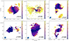 |
Fig. C.1. CO(2–1) velocity over velocity dispersion (v/σ) maps of the QSO2s. In the case of J1010 (top left panel) CO(3–2) has been used instead. The color bars indicate v/σ ranging from 0 to 10 and the dotted blue line shows the v/σ = 1 contour. The beam sizes are indicated by the blue ellipses at the bottom-left corner of each panel. |
All Tables
Position angles of the cold, warm molecular, and ionized outflows and radio jets.
All Figures
|
Fig. 1. ALMA CO(2–1) peak-intensity maps of the six QSO2s. The color bars indicate the scales of the flux density in mJy. The horizontal black lines indicate the physical scales for each galaxy, and the beam sizes are shown in the bottom left corner of each panel as red ellipses. The CO(2–1) distribution presents a variety of morphologies, such as spiral arms, double peaks, and merger signatures. East is to the left, and north is up. |
| In the text | |
|
Fig. 2. Moment maps of the CO(3–2) emission for the QSO2s. From left to right, the panels correspond to the peak intensities (in mJy units), the integrated intensity (moment 0, in Jy beam−1 km s−1 units), the intensity-weighted velocity field (moment 1, in km s−1), and the velocity dispersion (moment 2, in km s−1), respectively. East is to the left, and north is up. The red ellipses in the bottom left corner of the velocity dispersion maps indicate the beam sizes. The black stars show the nuclei, defined as the peak of the 220 GHz continuum as in RA22. For the cases of J1347 and J1356, a secondary nucleus (blue star) is identified in the optical and/or with ALMA continuum to the East and South directions, respectively. Green contours on the left panels indicate the ∼0 |
| In the text | |
|
Fig. 3. Brightness temperature ratio R32 and CO(2–1) and CO(3–2) velocity dispersion maps. The top panels show the R32 map at the coarser resolution of either CO(2–1) or CO(3–2), with the VLA 6 GHz HR contours overlaid in black (at 4, 8, 16, 32, and 64σrms, with σrms listed in Table A.1 in the appendix, also in Table 3 of Jarvis et al. 2019). For J1100 we present the e-MERLIN observations at 1.5 GHz at a 0 |
| In the text | |
|
Fig. 4. Position-velocity diagrams along the major (top panels) and minor (bottom panels) axis of the of the CO(3–2) emission (left) and the R32 line ratios (right) for J1010. The PVDs were extracted in a slit of 0 |
| In the text | |
|
Fig. 5. Same as Fig 4, but for J1100. The PVDs were extracted in a slit of 0 |
| In the text | |
|
Fig. 6. Same as Fig. 4, but for J1347. The PVDs were extracted in a slit of 0 |
| In the text | |
|
Fig. 7. Same as Fig. 4, but for J1356. The PVDs were extracted in a slit of 0 |
| In the text | |
|
Fig. 8. High-velocity flux maps overlaid on the CO velocity dispersion maps for the six QSO2s. The color maps corresponds to the moment 2 of the total CO(2–1) emission at 0 |
| In the text | |
|
Fig. 9. Outflow rate vs. bolometric luminosity. The molecular outflow mass rates derived for the QSO2s using the three scenarios are displayed as large purple circles for the intermediate value, and dashed black lines connecting the most and least conservative values (small purple circles). For comparison, we included other molecular mass outflow rates measurements from the literature as circles of different colors: AGN and ULIRGs from Fiore et al. (2017), QSO2s from Girdhar et al. (2024), two type-1 QSOs from Fei et al. (2024), AGN-dominated ULIRGs from Lamperti et al. (2022), AGN with possibly jet-driven outflows from Papachristou et al. (2023), and the low-power jet-driven outflow from Murthy et al. (2022). Mass outflow rates reported for ionized outflows in the literature are shown with different symbols and shades of blue: AGN and ULIRGs from Fiore et al. (2017) as squares, local jetted-Seyfert galaxies from Venturi et al. (2021) as upward triangles, QSO2s at z < 0.4 from Ulivi et al. (2024) as downward triangles, and four of the QSO2s studied here from Speranza et al. (2024) as diamonds. The corresponding linear fits from Fiore et al. (2017) are shown as a salmon dot-dashed line for molecular outflows and as a blue dashed line for the ionized ones. The mass outflow rates from the literature have been converted to the thin shell geometry adopted in this work when necessary. |
| In the text | |
|
Fig. 10. Kinetic power of the outflow vs. bolometric luminosity (left panel) and jet power (right panel). The 1:1, 1:100, and 1:1000 relations are shown as dashed lines in both panels. The dashed purple line in both panels corresponds to the linear fit of the purple circles, which correspond to the molecular outflows of the QSO2s studied here (“QSOFEED mol.”). The diverging color line (“Quasars mol.”) represents the linear fit of the type-1 PG quasars in Fei et al. (2024, green circles), the QSO2s from Girdhar et al. (2024, magenta circles), and the QSOFEED QSO2s (purple circles). The light orange dot-dashed line (“All molecular”) shows the fit of all the molecular outflows mentioned before and those reported by Papachristou et al. (2023, yellow circles) and Murthy et al. (2022, red circles). Symbols and colors are the same as in Figure 9. |
| In the text | |
|
Fig. 11. Histogram of the integrated R32 for the five QSO2s for which CO(2–1) and CO(3–2) transitions are available. They are shown as filled purple bars. The values measured for a sample of QSO2s at z < 0.2 from Molyneux et al. (2024) are also shown in light blue, for the X-ray selected AGN reported by Lamperti et al. (2020) in pink, of the local ULIRGs presented in Montoya Arroyave et al. (2023) in yellow, and the mean value measured for star-forming disk galaxies from Leroy et al. (2022) is the gray dot-dashed line, with the corresponding interval shown as a shaded gray area. |
| In the text | |
|
Fig. 12. Distribution of the R32 values in the PVD along the minor axis for the high-velocity (red) and disk regions (green) shown in Figures 4–7. |
| In the text | |
|
Fig. B.1. 3DBAROLO kinematic maps of the CO(3–2) emission of J1010. The panels on the left show the data, the middle panels show the best 3DBAROLO model, and the residuals (data-model) are shown on the right panels for the intensity (top row), velocity field (middle row), and velocity dispersion (bottom row). The cross represents the continuum peak at 200 GHz, and the PA of the kinematic major axis of the galaxy is indicated with dashed lines. |
| In the text | |
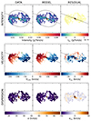 |
Fig. B.2. Same as Figure B.1, but for J1100. |
| In the text | |
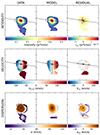 |
Fig. B.3. Same as Figure B.1, but for J1347. |
| In the text | |
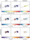 |
Fig. B.4. Same as Figure B.1, but for J1356. |
| In the text | |
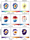 |
Fig. B.5. Same as Figure B.1, but for J1430. |
| In the text | |
|
Fig. C.1. CO(2–1) velocity over velocity dispersion (v/σ) maps of the QSO2s. In the case of J1010 (top left panel) CO(3–2) has been used instead. The color bars indicate v/σ ranging from 0 to 10 and the dotted blue line shows the v/σ = 1 contour. The beam sizes are indicated by the blue ellipses at the bottom-left corner of each panel. |
| In the text | |
Current usage metrics show cumulative count of Article Views (full-text article views including HTML views, PDF and ePub downloads, according to the available data) and Abstracts Views on Vision4Press platform.
Data correspond to usage on the plateform after 2015. The current usage metrics is available 48-96 hours after online publication and is updated daily on week days.
Initial download of the metrics may take a while.