| Issue |
A&A
Volume 695, March 2025
|
|
|---|---|---|
| Article Number | A185 | |
| Number of page(s) | 20 | |
| Section | Extragalactic astronomy | |
| DOI | https://doi.org/10.1051/0004-6361/202453224 | |
| Published online | 18 March 2025 | |
Unveiling the warm molecular outflow component of type-2 quasars with SINFONI
1
SISSA, Via Bonomea 265, I-34136 Trieste, Italy
2
INAF - Osservatorio Astrofisico di Arcetri, Largo E. Fermi 5, 50125 Firenze, Italy
3
INAF Osservatorio Astronomico di Trieste, via G.B. Tiepolo 11, 34143 Trieste, Italy
4
Instituto de Astrofísica de Canarias, Calle Vía Láctea, s/n, 38205 La Laguna, Tenerife, Spain
5
Departamento de Astrofísica, Universidad de La Laguna, 38206 La Laguna, Tenerife, Spain
6
Department of Physics & Astronomy, University of Alaska Anchorage, Anchorage, AK 99508-4664, USA
7
Department of Physics, University of Alaska, Fairbanks, Alaska 99775-5920, USA
8
Department of Physics and Astronomy, The University of Texas at San Antonio, 1 UTSA Circle, San Antonio, Texas 78249-0600, USA
9
IFPU - Institute for fundamental physics of the Universe, Via Beirut 2, 34014 Trieste, Italy
10
INAF, Istituto di Radioastronomia, Italian ARC, Via Piero Gobetti 101, I-40129 Bologna, Italy
11
INFN, Sezione di Trieste, via Valerio 2, Trieste I-34127, Italy
12
Astrophysics Research Cluster, School of Mathematical and Physical Sciences, University of Sheffield, Sheffield S3 7RH, UK
⋆ Corresponding author; This email address is being protected from spambots. You need JavaScript enabled to view it.
, This email address is being protected from spambots. You need JavaScript enabled to view it.
Received:
29
November
2024
Accepted:
17
February
2025
Abstract
We present seeing-limited (0.8″) near-infrared integral field spectroscopy data of the type-2 quasars, QSO2s, SDSS J135646.10+102609.0 (J1356) and SDSS J143029.89+133912.1 (J1430, the Teacup), both belonging to the Quasar Feedback, QSOFEED, sample. The nuclear K-band spectra (1.95–2.45 μm) of these radio-quiet QSO2s reveal several H2 emission lines, indicative of the presence of a warm molecular gas reservoir (T ≥ 1000 K). We measure nuclear masses of MH2 = 5.9, 4.1, and 1.5 × 10³ M⊙ in the inner 0.8″ diameter region of the Teacup (∼1.3 kpc), J1356 north (J1356N), and south nuclei (∼1.8 kpc), respectively. The total warm H2 mass budget is ∼4.5 × 10⁴ M⊙ in the Teacup and ∼1.3 × 10⁴ M⊙ in J1356N, implying warm-to-cold molecular gas ratios of 10−6. The warm molecular gas kinematics, traced with the H21-0S(1) and S(2) emission lines, is consistent with that of the cold molecular phase, traced by ALMA CO emission at higher angular resolution (0.2″ and 0.6″). In J1430, we detect the blue- and red-shifted sides of a compact warm molecular outflow extending up to 1.9 kpc and with velocities of 450 km s−1. In J1356 only the red-shifted side is detected, with a radius of up to 2.0 kpc and velocity of 370 km s−1. The outflow masses are 2.6 and 1.5 × 10³ M⊙ for the Teacup and J1356N, and the warm-to-cold gas ratios in the outflows are 0.8 and 1 × 10⁻⁴, implying that the cold molecular phase dominates the mass budget. We measure warm molecular mass outflow rates of 6.2 and 2.9 × 10⁻⁴ M⊙ yr−1 for the Teacup and J1356N, which are approximately 0.001% of the total mass outflow rate (ionized + cold and warm molecular). We find an enhancement of velocity dispersion in the H21-0S(1) residual dispersion map of the Teacup, both along and perpendicular to the compact radio jet direction. This enhanced turbulence can be reproduced by simulations of jet-ISM interactions.
Key words: galaxies: active / galaxies: evolution / galaxies: ISM / galaxies: individual: the Teacup / galaxies: nuclei / quasars: supermassive black holes
© The Authors 2025
 Open Access article, published by EDP Sciences, under the terms of the Creative Commons Attribution License (https://creativecommons.org/licenses/by/4.0), which permits unrestricted use, distribution, and reproduction in any medium, provided the original work is properly cited.
This article is published in open access under the Subscribe to Open model. This email address is being protected from spambots. You need JavaScript enabled to view it. to support open access publication.
1. Introduction
Strong observational evidence demonstrated that a tight relation exists between the properties of accreting super massive black holes, or SMBHs, and those of their hosting galaxies. Scaling relations have been identified among the SMBH mass and host galaxy properties, galaxy luminosity, bulge mass, velocity dispersion, and total stellar mass (e.g., Marconi & Hunt 2003; Häring & Rix 2004; Gültekin et al. 2009; Kormendy & Ho 2013). These scaling relations are due to the coevolution of accreting SMBHs (i.e., active galactic nuclei; AGN) and the host galaxy. However, the mechanisms driving this coevolution are not yet fully understood. The AGN can power strong winds and jets impacting on the galaxy interstellar medium, or ISM, altering both further star formation, abbreviated as SF, and nuclear gas accretion (see Harrison & Ramos Almeida 2024, for a recent review). SMBH growth and nuclear activity are then stopped, until new cold gas replenishes the nucleus, thus starting a new AGN phase, which gives rise to the feeding and feedback cycle (e.g., García-Burillo et al. 2021, 2024). Indeed, cosmological simulations require AGN feedback to regulate galaxy growth and reproduce the observed properties of massive galaxies (e.g., Schaye et al. 2015; Dubois et al. 2016; Nelson et al. 2018). Hence, the interplay between AGN-driven outflows and the host galaxy ISM lies at the core of the processes governing the coevolution of SMBHs and galaxies.
The primary feedback mechanisms are known as the quasar or radiative mode and the radio or kinetic mode. The quasar mode is believed to operate in AGN with high accretion rates, with the AGN energy producing gas outflows (Fabian 2012), while the radio mode is typically linked to powerful radio galaxies with lower accretion rates, where jets mechanically compress and accelerate the gas (McNamara & Nulsen 2007). However, the separation between the two feedback mechanisms is overly simplistic, as both modes can occur simultaneously. Not only powerful jets in radio-loud objects can accelerate powerful outflows (e.g., Nesvadba et al. 2008; Vayner et al. 2017; Coloma Puga et al. 2023, 2024), but outflows can also be accelerated by low power compact radio jets in galaxies typically classified as radio-quiet (Combes et al. 2013; García-Burillo et al. 2014; Harrison et al. 2015; Morganti et al. 2015; Jarvis et al. 2019; Audibert et al. 2019, 2023; Venturi et al. 2021; Girdhar et al. 2022). Moreover, AGN-driven outflows are almost ubiquitous and occur on a wide range of physical scales (Fiore et al. 2017; Lutz et al. 2020).
The ISM consists of a mixture of different gas phases, from the cold molecular and atomic to the warm ionized and hot X-ray emitting gas, and so are the outflows (Cicone et al. 2018; Harrison & Ramos Almeida 2024). However, the relationships between the different gas phases involved in the outflows, their relative weight, and impact on the galaxy ISM are largely unconstrained (Bischetti et al. 2019; Fluetsch et al. 2019). To date, there are only a few sources for which multiphase and multiscale outflows have been constrained simultaneously (e.g., García-Burillo et al. 2014; Cresci et al. 2015; Ramos Almeida et al. 2017, 2019; Venturi et al. 2018; Alonso-Herrero et al. 2018; García-Burillo et al. 2019; Rosario et al. 2019; Shimizu et al. 2019; Feruglio et al. 2020; García-Bernete et al. 2021; Speranza et al. 2022; Zanchettin et al. 2023). In some cases, molecular and ionized winds have similar velocities and are nearly co-spatial (Feruglio et al. 2018; Alonso-Herrero et al. 2019; Zanchettin et al. 2021), while more commonly, AGN show ionized winds that are faster than molecular ones (see Veilleux et al. 2020, and references therein).
Among the different gas phases involved in galactic outflows, the molecular phase is of particular significance, as it has been shown to dominate the mass of the outflow (Feruglio et al. 2010; Rupke & Veilleux 2013; Cicone et al. 2014; Carniani et al. 2015; Fiore et al. 2017; Fluetsch et al. 2021; Speranza et al. 2024). Furthermore, since the hydrogen molecule H2 is the fuel required to form stars and feed the SMBH, the impact of the outflows on this gaseous phase could really affect how systems evolve. Thanks to the synergy of the Atacama Large Millimeter/submillimeter Array, ALMA, with near- and mid-infrared integral observations such as VLT/SINFONI and the James Webb Space Telescope, JWST, it is now possible to probe the cold (CO) and warm (H2) molecular gas phases (e.g., Combes et al. 2014; Smajić et al. 2015; Pereira-Santaella et al. 2016; Ramos Almeida et al. 2017, 2019; Shimizu et al. 2019; Ramos Almeida et al. 2022; Alonso Herrero et al. 2023; Liu et al. 2023; Zanchettin et al. 2024). In the near-infrared, we can find both rotational and vibrational H2 lines that trace molecular gas at temperatures of ∼1000 K, whereas in the mid-infrared, the rotational H2 lines trace gas at hundreds of kelvin. Before JWST, only a few works studied warm molecular outflows using near-infrared observations (e.g., Rupke & Veilleux 2013; Ramos Almeida et al. 2017, 2019; Speranza et al. 2022; Riffel et al. 2023), and only in a few sources were warm molecular outflows detected (Rupke & Veilleux 2013; Ramos Almeida et al. 2019; Riffel et al. 2023). In fact, some AGN with reported ionized and CO outflows do not show a warm molecular gas counterpart (Ramos Almeida et al. 2017; Riffel et al. 2023). Riffel et al. (2023) found that 94% of their sample of 33 low-luminosity AGN present ionized outflows, while warm outflows were observed for 76% of them. Here we report deep SINFONI observations of two type-2 quasars with the aim of investigating their warm molecular gas content and kinematics.
The paper is organized as follows. Section 2 presents the main properties of the targets. Section 3 describes the VLT/SINFONI observational set-up and data reduction. Section 4 presents the main results, in particular the nuclear spectra, the warm molecular gas properties, and the H2 kinematics. In Sect. 5 we discuss our results, and in Sect. 6 we summarize the main results and present our conclusions. Throughout this work, we assume the following cosmology: H0 = 70.0 km s−1 Mpc−1, Ωm = 0.3, and ΩΛ = 0.7. We adopt the same cosmology and redshifts as those used by Speranza et al. (2024), hereafter SP24, of z = 0.1232 and 0.0851 for J1356 and the Teacup. The spatial scales are 2.213 and 1.597 kpc/″, respectively.
2. The targets
The two targets studied here, SDSS J135646.10+102609.0 (J1356) and SDSS J143029.89+133912.1 (J1430, the Teacup), are drawn from a complete sample of 48 type-2 quasars (i.e., obscured quasars; QSOs), the Quasar Feedback, QSOFEED, sample (see Ramos Almeida et al. 2022; Pierce et al. 2023; Bessiere et al. 2024). The QSO2s in the parent sample are luminous (L[OIII] > 108.5 L⊙) and nearby (z < 0.14), and hosted in massive galaxies (M∗ ∼ 1011 M⊙).
Our two targets have been studied across a wide range of wavelengths, showing evidence of outflowing gas in the cold molecular and warm ionized gas phases. Ramos Almeida et al. (2022), hereafter RA22, analyzed ALMA CO(2-1) data at ∼0.2″ resolution (370 pc at z ∼ 0.1), finding diverse CO morphologies. The molecular mass outflow rates reported in RA22 for J1356 and J1430, of 7.8 and 15.8 M⊙ yr−1, are lower than those expected from observational empirical relations (Cicone et al. 2014; Fiore et al. 2017; Fluetsch et al. 2019), considering their bolometric luminosities of 1045.54 and 1045.83 erg s−1 (SP24), suggesting that AGN luminosity alone does not guarantee the presence of powerful outflows. The ionized outflows of J1356 and J1430 have been studied using data from different facilities operating in both optical (Greene et al. 2012; Keel et al. 2012; Harrison et al. 2014; Fischer et al. 2018) and near-infrared, NIR, (Ramos Almeida et al. 2017, 2019). SP24 analyzed Integral Field Spectroscopy, IFS, observations of the [O III]λ5007Å emission line from the Multi-Espectrógrafo en GTC de Alta Resolución para Astronomía, MEGARA, instrument on the 10.4 m Gran Telescopio CANARIAS, GTC. In these two QSO2s SP24 reported the detection of the approaching and receding sides of the outflows. In the case of J1430 and J1356, which have extended radio emission despite being radio-quiet1, the ionized outflows are well aligned with the radio, suggesting that low-power jets (Pjet ∼ 1043 − 44 erg s−1) could be compressing and accelerating the ionized gas, although it is also possible, especially in the case of J1356, that the extended radio emission is due to shocks induced by the ionized outflow as it shocks the surrounding ISM (Fischer et al. 2023). In the case of Teacup, Audibert et al. (2023) studied the jet-ISM interaction using data from the Very Large Array, VLA, and ALMA CO, and they concluded, after comparing with tailored simulations of jet-ISM interactions, that the jet, almost coplanar with the CO disc, shocks the ISM and drives the molecular gas outflow.
2.1. The Teacup
J1430, known as the Teacup (Keel et al. 2012), has been the subject of numerous studies across multiple wavelength ranges, including X-rays (Lansbury et al. 2018), optical (Keel et al. 2012; Harrison et al. 2015; Villar-Martín et al. 2018; Venturi et al. 2023), near-infrared (Ramos Almeida et al. 2017), submillimeter (RA22, Audibert et al. 2023), and radio (Harrison et al. 2015; Jarvis et al. 2019). The host galaxy is a bulge-dominated system that shows evidence of past interactions, such as concentric shell structures and nuclear dust lanes (Keel et al. 2015). Ramos Almeida et al. (2017) detected ionized and coronal nuclear outflows lacking a warm molecular gas counterpart (i.e., broad component in the H2 line profile) based on the analysis of near-infrared IFS data obtained with VLT/SINFONI. Among the five QSO2s with detected cold molecular CO(2-1) outflows reported by RA22, the Teacup exhibits the most peculiar CO(2-1) morphology and disturbed kinematics. The CO outflow is compact (rout ∼ 0.5 kpc) and contains a cold molecular mass of 1.4 × 10⁷ M⊙, corresponding to a cold molecular mass outflow rate of 15.8 M⊙ yr−1. By combining ALMA CO(2-1) data with additional archival ALMA CO(3-2) observations, Audibert et al. (2023) identified evidence of jet-induced molecular gas excitation and turbulence perpendicular to the compact radio jet (spanning ∼0.8 kpc, PA = 60°) observed in VLA data at 0.25″ resolution (Harrison et al. 2015). Venturi et al. (2023) observed an enhanced ionized gas velocity dispersion perpendicular to the jet head using optical IFS data from VLT/MUSE. Furthermore, SP24, analyzing optical data from GTC/MEGARA, reported ionized outflow sizes of 3.1 and 3.7 kpc for the receding and approaching outflow sides, and outflow mass rates of 1.6–3.3 M⊙ yr−1 depending on the tracer used to estimate the electron density.
2.2. J1356
J1356 is hosted in a merger system that shows distorted optical morphology. The two nuclei (North and South, hereafter N and S) are separated by 1.1″ (2.4 kpc). The N nucleus is the QSO2, whose host galaxy is the dominant member of the merger and the brightest in both optical (Greene et al. 2012; Harrison et al. 2014) and molecular gas (Sun et al. 2014; RA22). Although J1356 is a massive eary-type galaxy, also known as ETG, with a stellar population dominated by old stars (Greene et al. 2009), the star formation rate, or SFR, of 69 M⊙ yr−1 RA22 is probably a consequence of the ongoing merger. In addition to N and S nuclei, a huge stellar feature named the western arm (W arm) was identified from the ALMA and HST morphologies. This merging component represents ∼32% of the total molecular mass in the system (Sun et al. 2014; RA22). J1356 was reported to host multiphase AGN driven outflows. RA22 detected a compact CO outflow in the inner ∼0.4 kpc with a mass outflow rate of approximately 8 M⊙ yr−1. Furthermore, SP24 reported ionized outflow sizes of 6.8 and 12.6 kpc for the receding and approaching outflow sides, and outflow mass rates of 1.2–6.1 M⊙ yr−1 depending on the tracer used to estimate the electron density.
3. Observations and data reduction
The Teacup and J1356 were observed in the K-band (1.95–2.45 μm) with the Very Large Telescope/Spectrograph for INtegral Field Observations in the Near Infrared, also known as VLT/SINFONI (Eisenhauer et al. 2003; Bonnet et al. 2004). Observations were carried out between April 2016 and August 2017 (Program ID: 097.B-0923(A); PI: J. Mullaney) in service mode. J1356 observations consist of 24 integrations of 147 s on-target, each carried out in 10 nights, for a total exposure time of 3528 s. The Teacup’s observations consist of 13 integrations of 147 s on-source, each carried out in 5 nights, for a total exposure time of 1911 s. To increase the signal-to-noise ratio of the Teacup’s dataset, we combined these data with those analyzed in Ramos Almeida et al. (2017) (Program ID: 094.B-0189(A); PI: M. Villar-Martín), obtaining a total exposure time of 3711 s, comparable to the exposure time of the J1356 observations. The observations are split into short exposures because of the strong and rapid variation of the infrared sky emission, following a jittering O-S-S-O pattern for object and sky frames. The observing conditions were clear and the seeing variation over the on-source observing periods was small and fullfilled the requested observing conditions (seeing < 0.8″ and an airmass < 2.0) according to the ESO astronomical site monitor2 and to our own measurements. To do so we took the cubes of the standard stars observed during the same nights as the science targets, and we collapsed them along the spectral axis. We then fitted a 2D Gaussian to the collapsed cubes to estimate the seeing FWHM and obtained average values of FWHM = (0.62″ ± 0.09″) × (0.51″ ± 0.09″) for the Teacup and FWHM = (0.71″ ± 0.15″) × (0.59″ ± 0.14″) for J1356.
We used the configuration 0.125″ × 0.250″ pixel−1, which produces a field-of-view, FOV, of 8″ × 8″ per single exposure. Thanks to the jittering process, the effective FOV in the case of Teacup and J1356, respectively, are 9″ × 8.5″ (14.4 kpc × 13.6 kpc) and 8.25″ × 10.25″ (18.3 kpc × 22.7 kpc). The channel width is 2.45 Å (∼30 km s−1) and the average spectral resolution in the K-band is ∼3300, which translates into a spectral resolution of ∼75 km s−1.
We adopted the already reduced and calibrated data from the 094.B-0189(A) program (see Ramos Almeida et al. 2017, for the details of the data observations and reduction) of the Teacup. For the other dataset 097.B-0923(A) we used the ESO Recipe Flexible Execution Workbench EsoReFlex (version 2.11.5), and the ESO Recipe Execution TooL EsoRex (version 3.13.8) to reduce the SINFONI data, and our own IDL routines for telluric correction and flux calibration. The ESO pipeline applies the usual calibration corrections of dark subtraction, flat-fielding, detector linearity, geometrical distortion, wavelength calibration, and subtraction of the sky emission to the individual frames. The flux-calibrated individual frames from multiple exposures were combined using the pipeline recipe sinfo_utl_cube_combine applying sigma clipping before coaddition (–ks_clip=TRUE), and by scaling the sky (using –scale_sky=TRUE) within individual exposures. If –scale_sky=TRUE, the spatial median of each cube plane is subtracted from all contributing cube planes before cube coaddition. This step removes sky background residuals that may not have been fully corrected during earlier data reduction stages (e.g., frame stacking), potentially caused by temporal sky variations.
4. Results
4.1. Nuclear spectra
We extracted the K-band spectra of the nuclear region of the Teacup, J1356N, and J1356S nuclei, using circular apertures of 0.8″ diameter (∼1.2 and 1.8 kpc for the Teacup and J1356, respectively), centered at the maximum of the Paα emission. The aperture was chosen to match the spatial resolution set by the seeing (< 0.8″). In the following, we will refer to the spectra extracted with this aperture as nuclear spectra, which are shown in Figure 1 with the emission lines labeled.
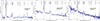 |
Fig. 1. Flux-calibrated nuclear spectra of the Teacup, J1356N and J1356S extracted in a circular aperture of 0.8″ diameter and smoothed using a 3 pixels boxcar. The most prominent emission lines are labeled. |
The most prominent emission features in the nuclear spectra of both galaxies are Paα, Brδ, HeIλ2.060 μm, Brγ, and the coronal line [Si VI] λ 1.963 μm. We also detect several H2 emission lines which are indicative of the presence of a nuclear warm molecular gas reservoir. We perform the fit of these emission lines adopting a combination of Gaussian profiles using the astropy Python library. In Figures 2, 3, and A.2, we show the profiles and corresponding fits of Paα, Brδ, Brγ, [SiVI], H21-0S(1), H21-0S(2) and H21-0S(3). In Tables 1 and A.1 we report the FWHMs, velocity shifts (Vs), and fluxes resulting from our fits with their corresponding errors. Velocity shifts are calculated with respect to the red-shifted central wavelength, assuming z = 0.1232 and 0.0851 for J1356 and the Teacup (SP24). The uncertainties in Vs include the wavelength calibration error (∼8 km s−1, as measured from the sky spectrum) and the individual fit uncertainties. In the case of fluxes, the errors have been determined by adding quadratically the flux calibration error (15%, Ramos Almeida et al. 2017) and the fit uncertainties. The FWHMs reported in Tables 1 and A.1 are corrected for instrumental broadening (∼75 km s−1).
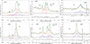 |
Fig. 2. Line profiles showing the nuclear spectra of J1356N (top panels) and the Teacup (bottom panels), extracted in a circular aperture of 0.8″ diameter and smoothed using a 3 pixel boxcar. The corresponding fits are shown as solid green lines. Solid blue and dot-dashed red Gaussians are the broad- and narrow- line components, respectively, and the orange dashed line is the continuum. The Gaussians have been vertically shifted for displaying purposes. The insets at the bottom of each panel are the residuals. The gray dotted vertical lines mark the expected position of the line peaks according to the redshift of the QSO2s. |
We require three Gaussians to reproduce the Paα line profile in J1356N nuclear spectrum. This includes two narrow blue- and red-shifted components of FWHM ∼ 400 km s−1 and a broad red-shifted component of FWHM ∼ 1280 km s−1. We also notice that the He I and He II lines, which are blended with Paα, require only one Gaussian with FWHM ∼ 600–750 km s−1. Similarly to Paα, we were able to fit the H21-0S(1) line profile with two narrow components (FWHM ∼ 450 and ∼265 km s−1), blue- and red-shifted with respect the systemic velocity calculated using the QSO2 redshift. Being a merging system, it is not surprising that this QSO2 shows complex and irregular gas kinematics. In fact, SP24 also reported evidence of two narrow, two intermediate, and one broad components in the [O III] doublet line profile traced by MEGARA, which has even higher spectral resolution than SINFONI. We identify the broad Paα component with the nuclear counterpart of the ionized outflow detected in [O III] for which SP24 reported a FWHM of ∼1300 km s−1. In the case of [SiVI], we fit a single red-shifted component of FWHM ∼ 890 km s−1 with Vs ∼ 230 km s−1. In the case of Brδ and the H21-0S(2), S(3), S(4), and S(5) molecular lines, single Gaussians with FWHM ∼ 500–740 km s−1 were sufficient to reproduce the profiles (see Table 1).
Emission lines detected in the nuclear spectrum of J1356N (0.8″ diameter).
In the case of J1356S, we require only one Gaussian to reproduce the line profiles in the nuclear spectrum (see Table A.1). In particular, the Paα, He I, and He II lines, which are blended together, are fitted with one Gaussian component of FWHM ∼ 700–940 km s−1. The [SiVI] line profile requires only one Gaussian with FWHM ∼ 940 km s−1 and Vs ∼ 50 km s−1. In the case of Brδ, a single Gaussian with FWHM ∼ 470 km s−1 and Vs ∼ −10 km s−1 was sufficient to reproduce the line profile. The H21-0S(1), S(2), S(3), S(4), and S(5) molecular lines are fitted with single Gaussians with FWHM ∼ 620–1175 km s−1 (see Table A.1). Finally, the Brγ emission line shows a low signal-to-noise ratio in the spectra of J1356, being at the edge of the SINFONI wavelength coverage. We fitted the line profile with a narrow Gaussian of FWHM ∼ 465 km s−1 and a broad one of ∼1410 km s−1 in J1356N spectrum, while in the case of J1356S the line appears undetected.
For what concerns the Teacup nuclear spectrum, we require two Gaussians to reproduce the [SiVI] line profile. This includes a narrow and broad component of FWHM ∼ 510 km s−1 and ∼1175 km s−1 respectively. Ramos Almeida et al. (2017) already detected a broad component of [SiVI] line at nucleus, which they identified with the coronal gas counterpart of the nuclear outflow detected with optical spectroscopic data (Villar Martín et al. 2014; Harrison et al. 2015). In the case of Paα, we fitted a narrow component of FWHM ∼ 420 km s−1 and a broad component of FWHM ∼ 1245 km s−1 blue-shifted by about 90 km s−1 with respect to the narrow component. This fit is not consistent with what was reported by Ramos Almeida et al. (2017), who measured a FWHM of the broad Paα of ∼1795 km s−1, likely due to the fact that the latter authors did not fit the He I and He II line profiles. To reproduce the profiles of He I and He II lines, we used only one Gaussian with FWHM ∼ 375 km s−1 and 550 km s−1, respectively. If we neglect the contributions of He I and He II and fit the Paα line profile with only a narrow and a broad component, we find FWHM ∼ 1655 km s−1 for the broad Paα component (see Appendix A and Figure A.1), which is consistent within 2σ with the FWHM reported by Ramos Almeida et al. (2017). In the case of Brδ, we fitted a broad component of FWHM ∼ 1180 km s−1 and Vs ∼ −200 km s−1 relative to the central wavelength of the narrow component. The Brγ line profile is well reproduced by a narrow and a broad component with FWHM ∼ 320 km s−1 and 950 km s−1, respectively. Finally, in the case of the molecular lines, as earlier, the line profiles are fitted by a single Gaussian with FWHM ∼ 480–600 km s−1 (Table A.1 and bottom panels of Figure 3).
4.2. The warm molecular gas
In the following, we will focus on the molecular H2 lines, which trace the warm molecular gas phase of the ISM. In fact, our goal is to characterize the properties and kinematics of warm molecular gas and to compare with the cold molecular gas phase traced with CO line and presented in RA22 and Audibert et al. (2023). Since the H21-0S(3) line is blended with [SiVI], we will focus the analysis on the H21-0S(1) and H21-0S(2) emission, being the other two most prominent H2 lines in the spectra.
We determine the mass of warm molecular gas measured from the nuclear spectra of the two QSO2s from the H21-0S(1) line luminosity and adopting the following relation from Mazzalay et al. (2013):
 (1)
(1)
where D is the luminosity distance and FH21 − 0S(1)corr is the extinction corrected H21-0S(1) line flux. The H21-0S(1) line fluxes are corrected for extinction using the infrared extinction AK, derived from the optical extinction AV assuming that AK ≈ 0.1 × AV. In the case of the Teacup we adopted the AV = 1.2 mag, which is the value measured in the same region from the VLT/MUSE data reported by Venturi et al. (2023). For J1356 we adopted AV = 0.9 mag from VLT/MUSE data of this galaxy (Bianchin et al. in prep.). Therefore, using Eq. (1) we measure MH2 = (5.85 ± 0.90) × 103 M⊙ in the Teacup for the central 0.8″ diameter. Ramos Almeida et al. (2017) reported MH2 ∼ 3 × 10³ M⊙ in an aperture of 0.5″ diameter and MH2 ∼ 10 × 103 M⊙ in an aperture of 1.25″. We find that the north nucleus is the brightest in H2, as it is also the case for CO and [O III] (RA22; SP24). For J1356N and J1356S, we measured MH2 = (4.05 ± 0.69)×103 M⊙ and (1.47 ± 0.37) × 103 M⊙ using the same aperture of 0.8″ diameter. According to our findings, J1356N contains the 75% of the warm molecular gas mass contained in the system. Therefore, in the following, the kinematic analysis will be focused on J1356N only, and we omit the N/North wording from this point onward.
We produced H21-0S(1) and S(2) integrated intensity (moment 0) maps of the Teacup and J1356, which are shown in the left and middle panels of Figure 4. In order to compare with the cold phase of the molecular gas, we also measured the total warm H2 masses. Thus, we extracted the H21-0S(1) emission from the line emitting regions above 2σ (see Figure 4), and we followed the procedure described above. We measured total warm molecular gas masses of MH2warm ∼ 4.5 and 1.3 × 10⁴ M⊙ for the Teacup and the J1356 system, respectively, with maximum spatial extents of the H21-0S(1) emission at 2σ, measured from the AGN position, of 4.8 kpc and 5.8 kpc.
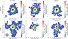 |
Fig. 4. Integrated intensity (i.e., moment 0) maps of the H21-0S(1), S(2), and stacked H2 of J1430 (top panels) and of J1356 (bottom panels). The black cross marks the peak of the near-infrared continuum. The maps have been smoothed using a two-spaxel boxcar for presentation purposes. Regions below 2σ are masked out. |
Furthermore, in order to increase the S/N of the molecular emission lines, we performed stacking of the two emission lines. Firstly, we cut the SINFONI data cubes around H21-0S(1) and S(2) emission lines, creating separate cubes for each line. We then modeled and subtracted the continuum for each spaxel individually. We removed the noise spikes by interpolating the spectrum of each spaxel. Then, we rebinned the spectra onto a common velocity grid centered on the observed wavelengths of each spectral line. We obtained continuun subtracted cubes for each line. We then created a weight map for each line by dividing the maximum intensity of the spaxel spectrum by the sum of the maxima of the two spectra. Finally, we normalized and combined the cubes using these weight maps. The right panels of Figure 4 show the moment 0 map of the stacked cube of the H2 lines of each QSO2.
The Teacup intensity map shows an elongated distribution of H2 at the nucleus, consistent with the S(1) intensity map shown in Ramos Almeida et al. (2017). The optical emission, both in continuum and in [O III], was reported to show a single-peaked compact morphology by several observations at different spatial resolutions (HST data at 0.1″, VLT/MUSE at 0.6″, MEGARA at 1.1″; Keel et al. 2012; Harrison et al. 2015; Venturi et al. 2023, SP24) On the contrary the morphology of the cold molecular gas, traced by CO(2-1) at 0.2″, shows a double peaked morphology, with the two peaks separated by ∼0.8″ (i.e., 1.3 kpc) with PA ∼ −10° (RA22; Audibert et al. 2023). resolution of the SINFONI data, we cannot resolve the two peaks. Ramos Almeida et al. (2017) reported that the H21-0S(1) emission is elongated by approximately 1.4 kpc along the N-S direction, roughly perpendicular to the Paα and [SiVI] emissions. In our H2 maps we observe the same, and thanks to the combination with new SINFONI observations, that is, increasing the exposure time by two times with respect to Ramos Almeida et al. (2017), we recover more extended H21-0S(1) diffuse emission. The H21-0S(2) emission shows a similar morphology, but is characterized by a lower S/N relative to H21-0S(1). Thanks to the stacking procedure, we can further investigate the diffuse emission of H2 by combining the two H2 lines. With respect to Ramos Almeida et al. (2017), we were able to recover emission up to 2″ (i.e., 3.2 kpc) along the E-W direction, and up to 3″ (i.e., 4.8 kpc) toward the south in the stacked moment map.
Focusing on J1356, we notice that the H21-0S(2) intensity peak is shifted by about 0.5″ in the south direction with respect to the H21-0S(1) intensity peak. In fact, the resulting map, obtained by stacking the two lines, shows a double peaked feature due to this mismatch between the S(1) and S(2) intensity peaks. J1356 shows an irregular and complex gas morphology, with the H21-0S(1) line showing elongated emission extending southward, exceeding 2″ (∼4.2 kpc) and also diffuse emission to the northeast and west regions of the map. The [O III] emission also appears elongated towards the south (SP24). In contrast, the S(2) emission is concentrated toward the center, with a maximum extension of ∼1.5″ (3.3 kpc), mainly in the northeast region of the map. The CO(2-1) emission is also quite compact, concentrated toward the central 0.5″ (∼1 kpc) radius region (RA22). Instead, the intensity map obtained from the stacked cube clearly shows that the diffuse emission is dominated by the H21-0S(1) line, exhibiting a similar morphology to the S(1) intensity map.
4.3. H2 kinematics
In order to interpret the warm molecular gas kinematics, we built a dynamical model of the systems fitting the observed H21-0S(1) data cubes with the 3D-Based Analysis of Rotating Objects from Line Observations (3DBAROLO, Di Teodoro & Fraternali 2015). We fit a 3D tilted-ring model to J1430 and J1356 H21-0S(1) data cubes using 0.4″ and 0.3″ wide annuli up to a maximum radial distance from the AGN of 1.6″ and 1.2″, respectively. In the first run, we allowed four parameters to vary: rotation velocity, velocity dispersion, disc inclination, and position angle, fixing the kinematic center to the peak position of the near-infrared continuum emission. For J1356, we ran the model again fixing the inclination to 52°, i.e., equal to the best fit disc inclination found by RA22, so that in this case only PA, rotation velocity, and velocity dispersion can vary. We follow this approach in this case because the inclination and position angle are strongly degenerate due to the lower S/N.
By subtracting the model velocity map from the observed one, we obtained mean-velocity residual maps that we used to investigate deviations from circular motions. We did the same with the velocity dispersion maps (see Figures 5 and 6). Finally, we produced position-velocity diagrams, abbreviated as PVDs, along the kinematics minor and major axis, adopting a slit width of 0.8″, i.e., equivalent to the spatial resolution of the SINFONI data cubes (see Figures 7 and B.1).
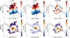 |
Fig. 5. H21-0S(1) moment 1 and 2 maps (i.e., velocity and velocity dispersion) of the Teacup. The 3DBAROLO models of the moment 1 and 2 maps and the corresponding residuals are also shown. Regions below 2σ are masked out. The black cross mark the peak of the near-infrared continuum as in Figure 4. The kinematic major axis is shown as a black dashed line in the moment 1 maps. The PAjet = 60° is indicated as a black solid line and gray shaded area. The maps have been smoothed using a two-spaxel boxcar for presentation purposes. North is up and east to the left. |
4.3.1. The Teacup
Figure 5 shows the H21-0S(1) velocity (moment 1) and velocity dispersion (moment 2) maps of the Teacup. As already reported by Ramos Almeida et al. (2017), the Teacup H21-0S(1) velocity field is dominated by rotation with a gradient approximately along the north-south direction and maximum velocities of ±250 km s−1. The rotation pattern is also clearly visible from the S-shaped structure in the PVD taken along PA = 13° ±6°, which is the kinematic major axis according to our modeling with 3DBAROLO (see Figure 7, top left panel). The H21-0S(1) moment 2 map shows high values of velocity dispersion up to ∼200 km s−1 in the central region and orthogonal to the radio jet orientation (PAjet = 60°), that decrease towards the outer regions. The kinematics maps shown in this work are overall consistent with those presented in Ramos Almeida et al. (2017) using VLT/SINFONI data and in RA22 and Audibert et al. (2023) using ALMA CO(2-1) and CO(3-2) data, respectively.
The moment 1 and 2 maps of J1430 3DBAROLO model and the corresponding residual moment maps (data-model) are shown in the middle and right panels of Figure 5. The 3DBAROLO disc model provides a position angle PA = 13° and inclination i = 42° as best fit parameters. Therefore, the kinematic major axis of the warm H2 gas disc differs from the CO major axis (PACO = 4°, RA22; Audibert et al. 2023), from the [O III] major axis (PA[OIII] = 27°, Harrison et al. 2014; Venturi et al. 2023; SP24), and from the galaxy major axis (PAgal = −19°). This could be related with the past merger event that Teacup undergone and/or with the influence of the jet on the ionized and molecular gas. The velocity residual moment map, shown in the top right panel of Figure 5, does not show strong residuals. The largest residuals are detected in the residual velocity dispersion map, shown in the bottom right panel of Figure 5, and they are located towards the southwest, along PA = 240°, which is the direction of the jet (PA = 60° = 240°).
Figure 7 shows the PVDs extracted from the H21-0S(1) cube: the left panels correspond to the PVDs extracted along the J1430 kinematic major (top) and minor (bottom) axis, and the middle panels to the PVDs extracted along (top) and perpendicular (bottom) to the jet direction. The blue and red contours trace the H21-0S(1) emission above 2σ in SINFONI data cube and 3DBAROLO model cube, respectively. Overall, the 3DBAROLO model reproduces well the kinematics of J1430. We consider as potential non circular motions only the gas emission outside 3DBAROLO contours at 2σ. In the case of the Teacup, these non circular motions are not very extended and for this reason we also considered the PVDs extracted from the stacked cube (see Figure B.1). The PVDs obtained along the kinematic major and minor axis show high velocity gas emission (v > |300| km s−1) within the central 1″ radius region that corresponds to non circular motions. In particular, red-shifted high velocity gas (v > 300 km s−1) is detected to the north along the kinematic major axis and to the west along the kinematic minor axis. In the PVDs extracted perpendicular to the jet direction from the stacked cube (bottom central panel of Figure B.1), we also to detect blue-shifted high-velocity gas (v < −300 km s−1) not accounted for by rotation. Furthermore, red-shifted gas at v ∼ 250 km s−1 outside 3DBAROLO contours is detected along the kinematic minor axis to the west, along the jet direction to the south-west, and perpendicular to the jet direction to the south-east.
4.3.2. J1356
The H21-0S(1) moment 1 and 2 maps of J1356 are shown in Figure 6, as well as the corresponding model and residual (data-model) moment maps. The H21-0S(1) moment 1 map shows positive velocities to the southeast and negative velocities to the northwest. The moment 2 data map shows high velocity dispersion values of up to 200 km s−1 in the center. Overall, the kinematics is quite complex and disturbed because of the ongoing merger.
The 3DBAROLO best-fit model is a rotating disc with a position angle PA = 121° ± 8° and inclination fixed to 52°, although as can be seen from the large residuals, the gas kinematics cannot be well reproduced by rotation. In this case the kinematic major axis is consistent with the CO major axis (PACO = 110°, RA22), therefore the H21-0S(1) and CO emission are tracing gas in the same disc. This warm and cold molecular gas is coplanar with the galaxy disc but has a different PA (igal = 55°, PAgal = 156°, RA22, from r-band SDSS DR6 photometry). In contrast, the [O III] kinematics is consistent with a rotation disc of kinematic major axis equal to 45° (Harrison et al. 2014; SP24). However, a misalignment between the galaxy and the nuclear molecular discs is not surprising in an ongoing major merger.
Large residual emission is shown in both moment 1 and 2 residual maps. The residual mean velocity map shows mainly red-shifted velocities concentrated toward the center. Similarly, the residual velocity dispersion map exhibits the strongest perturbations in the inner 1″ (∼2.2 kpc) radius region, reaching values of up to 100 km s−1. In fact, only the red-shifted side of the CO outflow was detected (RA22; Sun et al. 2014; Audibert et al. 2024). The right panels of Figure 7 show the H21-0S(1) PVDs obtained along the kinematic major (top) and minor (bottom) axis, and the same PVDs, but extracted from the stacked cube are shown in Figure B.1. As in the Teacup, we identify gas emission outside 3DBAROLO at the 2σ level as potential non circular motions. We detect high-velocity gas in the inner 0.8″ radius region, both along the kinematic major and minor axis. These high-velocity non circular motions have positive velocities, vmax ∼ 400 km s−1, as it was also the case for CO (RA22). Along the kinematics major axis to the west we barely resolve red-shifted low velocity gas, with v ∼ 100–200 km s−1, outside the 3DBAROLO model contours. However, we identify as outflow only the high-velocity non circular motions (see Section 4.4).
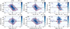 |
Fig. 7. PVDs extracted from the H21-0S(1) emission line data cubes. The blue contours trace the H21-0S(1) emission in SINFONI data cube, while the red contours trace the corresponding 3DBAROLO model. Left panels show the PVDs along the kinematic major (PA = 13°, top) and minor axis (PA = 103°, bottom) in J1430. Middle panels show the PVDs along (PA = 60°, top) and perpendicular (PA = 150°, bottom) to the radio jet direction in J1430. In the left and middle panels the blue and red contours are drawn at (2, 4, 8, 10)σ with σ = 3.23 10−19 W/m2/μm. Right panels: PVDs along the kinematic major (PA = 121°, top) and minor axis (PA = 211°, bottom) in J1356. The blue and red contours are drawn at (2, 3, 5)σ with σ = 3.26 10−19 W/m2/μm. All the PVDs were extracted using a slit of width 0.8″. |
4.4. Warm molecular outflows
In both QSO2s we detect high-velocity molecular gas that cannot be accounted for by rotation. This is evident from the PVDs reported in Figures 7 and B.1, where the SINFONI data (blue contours) exceeds 3DBAROLO disc model (red contours) at the same σ. In undisturbed spiral galaxies, such as the other two QSO2s studied by RA22, cold molecular outflows are usually coplanar with the CO discs, and non circular motions consistent with outflowing gas are usually found along the kinematic minor axis (e.g., RA22). However, as discussed in Audibert et al. (2023), in spheroidal galaxies which are undergoing or have undergone a galaxy interaction/merger, the molecular outflows might have a more 3D geometry and their preferential direction might not necessarily be the minor axis (see e.g., the case of the Teacup in CO). Therefore, here we follow the prescription from Scenario II described in Audibert et al. (2023) for measuring outflow masses.
We assume that only the high-velocity gas participates in the outflow, i.e., only the gas faster than the maximum velocity of the 3DBAROLO models at 2σ, shown in Figure 7. In the case of Teacup this corresponds to velocities larger than ±370 km s−1, and in J1356, to gas faster than 270 km s−1, without blue-shifted counterpart. Although we cannot discard that part of this high-velocity gas corresponds to complex motions associated with the mergers, specially in the case of J1356 (see RA22 and Audibert et al. 2024), here we assume that it corresponds to outflowing gas.
Then, to derive the outflow flux, we created integrated intensity maps by selecting only channels above these velocities and emission above 2σ. The velocity channel maps are shown in Figures B.2 and B.3, and the integrated intensity maps of the blue- and red-shifted high-velocity components are shown in Figure 8. We note that the integrated intensity outflow maps shown in Figure 8 and corresponding fluxes measured from them do not include the emission coming from spikes of noise that we spotted in the channel maps, which are probably residuals of sky subtraction. These noise spikes can be seen in the channel map at −491 km s−1 in the case of Teacup (to the south of the AGN; see Figure B.2) and in the channel maps at −463 and −324 km s−1 in J1356 (see Figure B.3). We computed the outflow masses from the extinction-corrected, integrated outflow flux, converting the H21-0S(1) line luminosity to warm molecular gas mass using Equation 1 and the infrared extinctions reported in Sect. 4.2. The corresponding values are shown in Table 2. For the outflows of Teacup and J1356 we measured total warm molecular gas masses of  and ∼1.5 × 10³ M⊙, which correspond to 44 and 37% of the mass of warm molecular gas measured in the central 0.8″ diameter of the galaxies, respectively.
Warm molecular outflow properties.
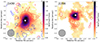 |
Fig. 8. Intensity maps of the high velocity components of the H21-0S(1) emission. The color map corresponds to the moment 0 of the total H21-0S(1) emission, while the contributions from high velocities are shown as red and blue contours. The spatial resolution of the SINFONI data is indicated with a gray ellipse in the bottom left corner. The white stars mark the peak of the near-infrared continuum as in Figure 4. Left panel: the red and blue contours of J1430 refer to velocities above ∼370 km s−1 with σred = 2.5 10−17 W/m2/μm.km s−1 and σblue = 2.7 10−17 W/m2/μm.km s−1. The red and blue contours are drawn at (2, 3,5, 7)σ. Right panel: the red contours of J1356 refer to velocities above ∼270 km s−1 with σred = 4.4 10−17 W/m2/μm.km s−1. The red contours are drawn at (2, 3, 4, 6)σ. |
In order to derive the outflow mass rates we assume a time-averaged thin expelled shell geometry and we adopted the following equation:
 (2)
(2)
In this equation Mout, vout, and rout are the outflow mass, velocity, and radius. We adopt as the outflow radius the maximum extent of the high-velocity gas contours at 3σ level shown in Figure 8, while the outflow velocity is the luminosity-weighted average of the velocity channels adopted to derive the integrated outflow flux as in RA22 and Audibert et al. (2023). For the Teacup, from Figure 8 we measure outflow radii of 1.2″ (1.9 kpc) for the blue- and red-shifted sides of the outflow, and outflow velocities of −470 km s−1 and 430 km s−1. From this we measure warm molecular outflow rates of 4.2 × 10⁻⁴ M⊙ yr−1 and 2.0 × 10⁻⁴ M⊙ yr−1, for the blue- and red-shifted sides of the outflow.
For J1356, we measure an outflow velocity of 370 km s−1 for the red-shifted side of the outflow. From the red contours in Figure 8 we measure an outflow radius of 0.9″ (2.0 kpc). From this we measure a warm molecular outflow rate of 2.9 × 10⁻⁴ M⊙ yr−1 for the red-shifted side of the outflow. Finally, we calculate the kinetic power of the warm molecular outflow as follows:
 (3)
(3)
With the above assumptions, we derive kinetic powers of log Ėkin/(erg s−1) ∼ 35 for both the two QSO2s. The summary of the outflow properties is reported in Table 2. Taking into account the total warm mass outflow rate of the Teacup of 6.26 M⊙ yr−1, we obtain a total kinetic power log Ėkin/(erg s−1) = 35.6 for the warm molecular outflow.
5. Discussion
In the present work, our aim is to complete the picture of the multiphase quasar-driven outflows for our QSO2s by adding the warm molecular measurements obtained in the near-infrared domain with SINFONI. We note that these warm molecular outflows are not detected in the nuclear spectra of the QSO2s shown in Figures 2 and 3. This is because the amount of molecular gas participating in the outflow is small, the velocities are not high, and the signal-to-noise of the nuclear spectra at the reddest wavelengths is relatively low. Thanks to the analysis of the integral field data that we have done, including the fits with 3DBAROLO and inspection of the PVDs, the warm molecular outflows were revealed.
Hereafter we compare the warm molecular gas properties with cold molecular ones. Then we discuss the contribution of the warm molecular phase to the multiphase outflow, its impact on the galaxy host, and the interplay of the compact radio jets with the gas of the ISM.
5.1. H2 gas properties and kinematics
In Sect. 4.2 we analyzed the nuclear spectra of the Teacup and of the two nuclei of J1356, finding that warm molecular gas masses of MH2warm ∼ 5.9, 4.1, and 1.5 × 10³ M⊙ in the central 0.8″ regions of J1430, J1356N, and J1356S, respectively. In the same Section, we also measured the total warm H2 masses that we can compare with the cold phase of the molecular gas. RA22 reported MH2cold ∼ 6.2 and 11.5 × 10⁹ M⊙ from the CO(2-1) emission of J1430 and J1356, respectively, with maximum radii of 0.8 and 2.3 kpc. These findings result in total warm-to-cold molecular gas ratios of 7 × 10⁻⁶ and 1 × 10⁻⁶ for the Teacup and J1356, respectively. Indeed, only a small fraction of the molecular gas reservoir in galaxies is expected to be found in the warm molecular phase of the ISM (e.g., Dale et al. 2005; Mazzalay et al. 2013). A warm-to-cold mass ratio of 6 − 7 × 10⁻⁵ was measured in two nearby Luminous Infrared Galaxies, or LIRGs, with (Pereira-Santaella et al. 2016) and without (Emonts et al. 2014) nuclear activity, combining NIR and sub-mm observations. Recently, García-Burillo et al. (2024) reported warm-to-cold molecular gas mass fractions ≤10−4, measured on nuclear scales in a sample of 45 nearby AGN (DL = 7–45 Mpc).
In Sect. 4.3 we modeled the H21-0S(1) kinematics with 3DBAROLO tilted disc models. In the Teacup we find that the CO and the warm H2 disc have the same inclination but different PA. Indeed, our best fit 3DBAROLO model provides a PA of the warm H2 disc of 13°, which lies in between the findings for the CO (PACO = 4°, RA22; Audibert et al. 2023), and the [O III] disc (PA[OIII] = 27°, Harrison et al. 2014; Venturi et al. 2023; SP24). The small difference between CO and warm H2 PA could be of low significance, as high uncertainties affect PA and inclination values, which can be highly degenerate. However, the major axis of the galaxy, PAgal = −19°, is highly inconsistent with the above values. These differences could be due to a warp in the discs and/or to disturbed motions which could be related to the past merger event and/or to the influence of the radio jet on the gas morphology and kinematics (Audibert et al. 2023; SP24).
J1356 is hosted in an ongoing merger system and thus, its kinematics is more disturbed. We found that the CO and the warm H2 major axis have consistent PA, therefore the two gas phases seem to trace the same disc. These warm and cold H2 discs are coplanar with the galaxy but have a different PA, which is not surprising in a merger.
In both QSO2s, the H21-0S(1) velocity gradient ranges are consistent with the CO velocity gradients (RA22, shown in their Figures 9 and 11), with maximum values of ±250 km s−1 in the Teacup and of ±200 km s−1 in J1356 (see Figures 5 and 6). On the contrary the H21-0S(1) moment 2 maps show velocity dispersion values of up to 200–250 km s−1 at the center, which are higher than the 120–160 km s−1 values shown in CO moment 2 maps (RA22, Figures 9 and 11). This difference could be related to the different spatial resolution of the two observations, but is more likely due to the higher temperature and lower density of the warm gas, which is usually characterized by a higher velocity dispersion (see García-Burillo et al. 2024, and references therein).
Finally, we detect a double-peaked emission line profile in both Paα and H21-0S(1) in the J1356N nuclear spectra shown in Figures 2 and 3. This is not detected in the CO(2-1) line profile shown in Figure 15 of RA22. Double peaked profiles can arise from the approaching and receding sides of a rotating gas disc or correspond to non-circular motions, sometimes associated with mergers (Maschmann et al. 2023). Furthermore, as can be seen from Figure 4, we also detect a shift in the H21-0S(1) and S(2) emission peaks that could be related to the ongoing merger and/or to the radio jet interaction with the ISM. However, higher spatial resolution data for both radio emission and molecular H2 lines are needed to distinguish between the different scenarios.
5.2. The multiphase outflow
We detected blue- and red-shifted high-velocity warm H2 gas in the nuclear region of the Teacup up to a radius of 1.9 kpc. In J1356 only the receding side of the warm H2 outflow is detected up to 2.0 kpc from the AGN. We identified this gas as the warm component of the multiphase outflows, whose ionized (Greene et al. 2012; Ramos Almeida et al. 2017; Venturi et al. 2023; SP24) and cold molecular (RA22; Audibert et al. 2023; Girdhar et al. 2024) phases have been discussed in previous works. In particular, using the CO(2-1) transition observed with ALMA at 0.2″ resolution, RA22 detected spatially resolved cold molecular outflows of 0.5 and 0.4 kpc in J1430 and J1356, respectively. For the same objects SP24 detected, using MEGARA observations of the [O III] line at 1.2″ resolution, ionized outflows which extend on galactic scales, from 3 kpc up to 13 kpc. Table 3 reports the cold molecular and warm ionized outflow properties of the two QSO2s (RA22; Audibert et al. 2024; SP24). Considering the warm and cold molecular outflow masses reported in Table 3, we derive warm-to-cold molecular gas ratios of ∼1 ×10⁻⁴ if we use the outflow masses from RA22 and of ∼1 ×10⁻⁵ if we use the values corresponding to Scenario II from Audibert et al. (2024). The cold molecular outflow masses were computed adopting a CO-to-H2 conversion factor αCO = 0.8 M⊙(K km s−1)−1, while the total cold molecular masses MH2cold were estimated using αCO = 4.35 M⊙(K km s−1)−1 (RA22). The ionized outflows of J1430 and J1356 have masses of 5 and 35 × 106 M⊙, respectively (see Table 3 and SP24) therefore, this gas phase is the fastest, but the cold molecular phase dominates the mass budget of the outflow. Indeed, in the local Universe and at AGN luminosities below 1047 erg s−1, it has been widely reported that molecular outflows carry more mass than their ionized counterparts (e.g., Veilleux et al. 2020; Feruglio et al. 2010; Rupke & Veilleux 2013; Cicone et al. 2014; Carniani et al. 2015; Fiore et al. 2017; Fluetsch et al. 2021).
Multiphase outflows properties
In this work we measured warm molecular outflow rates of 6.2 and 2.9 × 10⁻⁴ M⊙ yr−1 in the Teacup and J1356, which are consistent with the estimates available in the literature for other AGN of different luminosities, which range between 10−5 and 10−2 M⊙ yr−1 (Diniz et al. 2015; Ramos Almeida et al. 2019; Riffel et al. 2020; Bianchin et al. 2022; Riffel et al. 2023). In Riffel et al. (2023), whose warm molecular outflow compilation is the largest available in the local Universe to date, they characterized the H21-0S(1) emission and kinematics using data obtained with Gemini/NIFS of a sample of 33 AGN hosts with 0.001 < z < 0.056 and hard X-ray luminosities 41 < log LX/(erg s−1) < 45. They reported warm outflow masses of 100 − 104 M⊙ and warm molecular outflow rates of 10−5 − 10−2 M⊙ yr−1.
The warm molecular outflow mass rates reported in this work and the value measured for the QSOFEED QSO2 J1509+0434 (0.001 M⊙ yr−1, Ramos Almeida et al. 2019) can be compared with the cold molecular and warm ionized gas outflows reported for them by RA22, Audibert et al. (2024), and SP24. These are ṀCO = 7.8–41.0 M⊙ yr−1 and Ṁ[OIII] = 1.1–2.0 M⊙ yr−1 (see Table 3). In the comparison between the different outflow phases, it should be noted that the observations were carried out at different angular resolutions (0.2″, 1.2″, and 0.8″ in the case of ALMA, MEGARA, and SINFONI, respectively) and that different methodologies were employed to derive the outflow properties. RA22 identified as outflow only the high-velocity gas detected along the kinematic minor axis showing deviations from the circular motions modeled with 3DBAROLO. Audibert et al. (2023), considering four different scenarios to calculate the outflow mass rates of the Teacup using the same CO(2-1) data analyzed by RA22, reported values of ṀCO from 6.7 to 44 M⊙ yr−1. Table 3 reports the CO outflow properties derived by Audibert et al. (2024) for the two QSO2s studied here. The authors used the same method of this work, Scenario II from Audibert et al. (2023), and the same CO(2-1) data analyzed by RA22. We note that in the case J1356N, only the red-shifted side of the cold molecular outflow was detected (RA22; Sun et al. 2014; Audibert et al. 2024).
SP24 derived the ionized outflow properties by integrating all the high-velocity [OIII] emission above 3σ, and reported the detection of both the blue-shifted and red-shifted sides of the ionized outflows for Teacup and J1356. Taking into account the caveats mentioned above (see also Hervella Seoane et al. 2023), we can compare our values with those of the ionized and cold molecular gas, and we find that the relative contribution of the warm molecular phase to the total (i.e., ionized + warm molecular + cold molecular) mass outflow rate is approximately 0.001%. Figure 9 shows the relative contribution of the ionized, cold, and warm molecular phases to the total mass outflow rate in J1356 and the Teacup and, for the sake of completeness, in J1509 and J1100, which are also part of the QSOFEED sample. We note that the relative contribution of the ionized and cold molecular phases varies among the sources, while the contribution of the warm molecular phase is in the range 0.001–0.005%. The higher relative contribution of warm molecular outflowing gas is the one found in J1509 by Ramos Almeida et al. (2019), who detected outflows in both the ionized and warm molecular gas phases, analyzing near-infrared spectroscopic data from the Espectrógrafo Multiobjeto Infra-Rojo, or EMIR, instrument on the GTC. From the H21-0S(1) line luminosity they obtained an outflow mass of ∼104 M⊙, a factor 100–400 lower than the mass of the ionized outflow, and a mass outflow rate of 0.001 M⊙ yr−1 with an outflow radial size (FWHM) of ≈1.5 kpc.
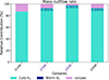 |
Fig. 9. Relative contribution of the cold molecular (turquoise), ionized (pink), and warm molecular (blue) phases to the total mass outflow rate. The blue labels refer to the relative contribution of the warm molecular phase in %. The galaxies whose names are in violet are the targets of this work. The ionized mass outflow rates are from SP24, adopting their [S II]-based electron densities and divided by us by a factor of 3 to match our outflow geometry. The cold molecular mass outflow rates are from Scenario II in Audibert et al. (2024), and the warm molecular mass outflow rate of J1509 is from Ramos Almeida et al. (2019). No warm molecular outfflow detections are yet reported for J1100. |
In this work, we aimed to provide a more comprehensive view of quasar-driven outflows by putting together the cold and warm molecular and warm ionized outflow measurements available for these QSOFEED quasars. Indeed, having a large sample with multiphase outflow measurements for the same targets is the ultimate goal of the QSOFEED project (RA22). It is worth mentioning that measurements of warm molecular gas outflows are scarce in the literature and that, at least in nearby AGN (z < 0.002), the warm molecular gas emission seems to be dominated by galaxy rotation (Davies et al. 2014, 2024; Riffel et al. 2018; Storchi-Bergmann & Schnorr-Müller 2019; Esparza-Arredondo et al. 2025). In fact, Ramos Almeida et al. (2017) did not report evidence of broad H2 components in the nuclear spectrum of the Teacup, with the velocity map showing a dominant rotation pattern. They addressed as possible signatures of outflowing molecular gas the nuclear narrow components blue-shifted with respect to the systemic velocity. Thanks to the deeper SINFONI observations analyzed here, we increased the exposure time by two times compared to the data analyzed in Ramos Almeida et al. (2017), and we were able to resolve the warm molecular outflow, which extends up to 1.9 kpc. The higher-sensitivity of JWST and its near- and mid-infrared instruments will surely contribute to increase number of warm molecular outflows detected in AGN.
5.3. The interaction of the outflow with the galaxy host
Using the SFRs measured for our two QSO2s reported by SP24, of 69 and 12 M⊙ yr−1, we can calculate the mass loading factor, η = Ṁout/SFR, for the warm molecular gas. We find η = 5.2 × 10⁻⁵ for the Teacup and η = 4.2 × 10⁻⁶ for J1356, which are rather small values. By combining our loading factors with those of the cold molecular phase and ionized gas, we obtain ηtot > 1 only for the Teacup, as already reported by RA22 and SP24. This suggests that in J1356, the star formation process is more effective in removing gas than the outflows. As discussed in SP24, it would be more accurate to compare the multiphase mass outflow rates with the SFRs calculated in the same regions. Here we are using SFRs derived from total far-infrared luminosity, representing a galaxy-wide SFR. The outflows, on the other hand, are more compact, especially in the case of the molecular outflows, which have radii of 0.4–0.5 kpc (RA22) and of 1.2–1.3 kpc (Audibert et al. 2024) for the cold molecular phase and of 1.9–2.0 kpc for the warm molecular phase. Another point to consider are the different timescales of star formation and outflows. Given that QSO2 outflows have dynamical timescales of approximately 1-20 Myr (see Table 3 and RA22; SP24; Bessiere & Ramos Almeida 2022; Audibert et al. 2024), their characteristics should be compared to those of recent star formation, which can be probed through resolved stellar population analysis (Bessiere & Ramos Almeida 2022) or through polycyclic aromatic hydrocarbon, or PAH, emission features detected in the mid-infrared, which are related to young and massive stars. (García-Bernete et al. 2022, 2024; Lai et al. 2022, 2023; Zhang et al. 2024; Ramos Almeida et al. 2023; Zanchettin et al. 2024). Indeed, the spatial distribution of PAHs in the two QSO2s will be studied thanks to available Cycle 2 JWST observations (PI: Ramos Almeida, proposal 3655). This approach will allow us to determine whether the outflows inhibit or stimulate recent star formation, or if both processes can occur simultaneously (Cresci et al. 2015; Carniani et al. 2016; Bessiere & Ramos Almeida 2022).
The two QSO2s analyzed in this work are radio-quiet objects with AGN luminosities of 1045.83 erg s−1 (The Teacup) and of 1045.54 erg s−1 (J1356), derived by SP24 from the extinction correct [O III] luminosities reported by Kong & Ho (2018). Therefore, the multiphase gas outflows should in principle be driven by radiation pressure and/or wind angle winds, typical of the quasar-mode feedback (Fabian 2012). However, it has been widely suggested that low-power compact jets in radio-quiet AGN can compress and shock the surrounding gas as they expand, contributing to the driving of both ionized and molecular outflows (e.g., Venturi et al. 2018; Jarvis et al. 2019; Audibert et al. 2023). The two QSO2s have 6 GHz VLA observations at both high (∼0.25″ beam) and low (∼1″ beam) angular resolutions, which were analyzed by Jarvis et al. (2019). The authors inferred that only a small fraction, i.e., 3–6%, of the radio emission is due to the star formation process. They identified the extended radio emission with a jet or a lobe in J1430, while the radio emission identification as a jet or a lobe is more tenuous in J1356, where the extended radio feature is only visible in the low-resolution map. SP24 noted that the red-shifted counterpart of J1356 ionized outflow, which extends up to ∼6.8 kpc is perfectly aligned with the 6 GHz radio contours at 1″ resolution, constituting a possible evidence for a jet-like structure accelerating the ionized gas through the galaxy ISM or to shocks induced by the outflow itself, which are seen in the radio (Fischer et al. 2023). However, due to the compactness of the warm molecular outflow detected with the SINFONI data, it is quite challenging to link the properties of the warm molecular outflow with the extended radio emission reported by Jarvis et al. (2019).
As for the Teacup, the high-angular resolution 6 GHz VLA observations reveal the presence of a compact radio jet along a PA = 60°, extending up to ∼0.8 kpc (Harrison et al. 2015; Jarvis et al. 2019), with a jet power of Pjet ∼ 1043 erg s−1 (Audibert et al. 2023). This compact jet-like structure seems to subtend a small angle relative to the cold molecular gas disc, and consequently to the warm molecular gas as well. Our H21-0S(1) residual dispersion map, shown in Figure 5, shows enhanced velocity dispersion in the south and southwest direction, both along and perpendicular to the jet direction. Additionally, PVDs along and perpendicular to the jet direction (see middle panels of Figures 7 and B.1) show non circular red-shifted emission at modest velocities, i.e., 50–250 km s−1 to the southwest and southeast. According to simulations (Mukherjee et al. 2018; Meenakshi et al. 2022), radio jets can efficiently inject kinetic energy into the surrounding gas, inducing local turbulence and shocks when the jets have a low inclination relative to the gas disc, as in the case of the Teacup. Audibert et al. (2023) performed a comparison between ALMA CO(2-1) and CO(3-2) observations and the simulations in Mukherjee et al. (2018), finding that the jet compresses and accelerates the molecular gas, driving a lateral outflow characterized by increased velocity dispersion and higher gas excitation.
The results presented here, along with those presented in previous studies of the same targets, might indicate that compact, low power jets could also be an efficient outflow driving mechanism even in radio-quiet AGN. This might contribute to explaining the dispersion in the Ṁout − Lbol plane found in recent studies (e.g., RA22; Lamperti et al. 2022). In the particular case of warm molecular outflows, kiloparsec scale radio/sub-mm continuum emission is detected in the three quasars with outflow measurements (J1430, J1356, and J1509), indicating a potential causal connection between the two. However, another quasar belonging to the QSOFEED sample, J0945 (Speranza et al. 2022) also shows extended (∼1 kpc) radio emission and no warm molecular outflow was found from the analysis of high angular resolution Gemini/NIFS observations. The orientation between the jets and the molecular gas discs could be a determinant factor here (Harrison & Ramos Almeida 2024).
6. Conclusions
In this paper we investigate deep near-infrared IFS data obtained with VLT/SINFONI of the type-2 quasars J1356 and J1430. We analyze the gas dynamics in the two systems, by using the H21-0S(1) and S(2) emission lines detected in the QSO2 spectra. We detect warm molecular outflows with radii of up to 2.0 and 1.9 kpc, respectively, but contributing very little to the total mass budget. We summarize our main findings as follows.
-
The warm molecular gas phase in the Teacup and in J1356 represents a small fraction of the total molecular gas. We measure masses of (5.85 ± 0.90) × 103 M⊙, (4.05 ± 0.69) × 103 M⊙, and (1.47 ± 0.37) × 103 M⊙ in the inner 0.8″ diameter region of the Teacup, J1356 north and south nuclei, respectively. The total warm H2 masses are ∼4.5 × 10⁴ M⊙ and ∼1.3 × 10⁴ M⊙ in the Teacup and in J1356, with maximum radii of 4.8 and 5.8 kpc. Considering the CO-derived masses of cold molecular gas of these QSO2s, this implies warm-to-cold molecular gas ratios of 7 and 1 ×10⁻⁶, respectively.
-
In the Teacup, the kinematics of the warm molecular gas is consistent with rotation, but the warm H2 PA differs from the galaxy PA, probably related to the past merger and/or to the influence of the jet on the ionized and molecular gas. In J1356 only a fraction of the warm molecular gas is rotating and the kinematics is disturbed, but the CO and warm H2 PAs are consistent, suggesting that are tracing the same disc. In both QSO2s, the H21-0S(1) emission shows higher velocity dispersion at the nucleus compared to CO.
-
In both QSO2s, high-velocity gas is detected, indicating the presence of warm molecular outflows, with velocities of 370 and 450 km s−1 and outflow masses of 1.5 and 2.6 × 10³ M⊙ for J1356 and the Teacup, respectively. The warm-to-cold gas ratios that we measure in the outflow regions are ∼1 × 10⁻⁵, which are significantly higher than the value measured in the central 0.8″ radius (1.8 and 1.3 kpc).
-
We measure warm molecular mass outflow rates of 6.2 × 10⁻⁴ M⊙ yr−1 and of 2.9 × 10⁻⁴ M⊙ yr−1 in J1430 and J1356, respectively, which are approximately 0.001% of the total (i.e., ionized + cold molecular + warm molecular) mass outflow rate. Adopting the SFRs derived from the total far-infrared luminosity, we measure mass loading factors of η = 5.2 × 10⁻⁵ for the Teacup and of η = 4.2 × 10⁻⁶ for J1356.
-
We detect an enhancement of velocity dispersion in the H21-0S(1) residual dispersion map of the Teacup, both along and perpendicular to the direction of the compact radio jet, approximately 1″ (∼1.6 kpc) from the AGN. This local turbulence could be due to the injection of kinetic energy from the radio jet, as already suggested by the comparison of the CO emission with simulations.
This study aimed to expand our understanding of multiphase quasar-driven outflows in our QSO2 by including warm molecular gas observations obtained in the near-infrared with VLT/SINFONI. Our findings reveal that the warm molecular gas, both in the disc and outflows, represents only a minor fraction of the total gas reservoir (considering warm ionized, cold molecular, and warm molecular phases and excluding the neutral gas phase).
Less than 7% of these two and other nearby QSO2s radio emission is associated with star formation, with non thermal AGN emission being responsible for the bulk of radio emission (Jarvis et al. 2019).
Acknowledgments
Based on observations made with ESO Telescopes at the Paranal Observatory under programs ID 097.B-0923(A) and 094.B-0189(A). Maria Vittoria Zanchettin acknowledges financial support from the PRIN MIUR 2017PH3WAT contract, and PRIN MAIN STREAM INAF “Black hole winds and the baryon cycle”. Cristina Ramos Almeida, Jose Acosta-Pulido, Anelise Audibert and Pedro Cezar acknowledge support from the Agencia Estatal de Investigación of the Ministerio de Ciencia, Innovación y Universidades (MCIU/AEI) under the grant “Tracking active galactic nuclei feedback from parsec to kiloparsec scales”, with reference PID2022−141105NB−I00 and the European Regional Development Fund (ERDF).
References
- Alonso-Herrero, A., Pereira-Santaella, M., García-Burillo, S., et al. 2018, ApJ, 859, 144 [Google Scholar]
- Alonso-Herrero, A., García-Burillo, S., Pereira-Santaella, M., et al. 2019, A&A, 628, A65 [NASA ADS] [CrossRef] [EDP Sciences] [Google Scholar]
- Alonso-Herrero, A., García-Burillo, S., Pereira-Santaella, M., et al. 2023, A&A, 675, A88 [NASA ADS] [CrossRef] [EDP Sciences] [Google Scholar]
- Audibert, A., Combes, F., García-Burillo, S., et al. 2019, A&A, 632, A33 [NASA ADS] [CrossRef] [EDP Sciences] [Google Scholar]
- Audibert, A., Ramos Almeida, C., García-Burillo, S., et al. 2023, A&A, 671, L12 [NASA ADS] [CrossRef] [EDP Sciences] [Google Scholar]
- Audibert, A., Ramos Almeida, C., García-Burillo, S., et al. 2024, A&A, submitted [Google Scholar]
- Bessiere, P. S., & Ramos Almeida, C. 2022, MNRAS, 512, L54 [NASA ADS] [CrossRef] [Google Scholar]
- Bessiere, P. S., Ramos Almeida, C., Holden, L. R., Tadhunter, C. N., & Canalizo, G. 2024, A&A, 689, A271 [NASA ADS] [CrossRef] [EDP Sciences] [Google Scholar]
- Bianchin, M., Riffel, R. A., Storchi-Bergmann, T., et al. 2022, MNRAS, 510, 639 [Google Scholar]
- Bischetti, M., Maiolino, R., Carniani, S., et al. 2019, A&A, 630, A59 [NASA ADS] [CrossRef] [EDP Sciences] [Google Scholar]
- Bonnet, H., Abuter, R., Baker, A., et al. 2004, The Messenger, 117, 17 [NASA ADS] [Google Scholar]
- Carniani, S., Marconi, A., Maiolino, R., et al. 2015, A&A, 580, A102 [NASA ADS] [CrossRef] [EDP Sciences] [Google Scholar]
- Carniani, S., Marconi, A., Maiolino, R., et al. 2016, A&A, 591, A28 [NASA ADS] [CrossRef] [EDP Sciences] [Google Scholar]
- Cicone, C., Maiolino, R., Sturm, E., et al. 2014, A&A, 562, A21 [NASA ADS] [CrossRef] [EDP Sciences] [Google Scholar]
- Cicone, C., Brusa, M., Ramos Almeida, C., et al. 2018, Nat. Astron., 2, 176 [Google Scholar]
- Coloma Puga, M., Balmaverde, B., Capetti, A., et al. 2023, ApJ, 958, L36 [NASA ADS] [CrossRef] [Google Scholar]
- Coloma Puga, M., Balmaverde, B., Capetti, A., et al. 2024, A&A, 686, A220 [NASA ADS] [CrossRef] [EDP Sciences] [Google Scholar]
- Combes, F., García-Burillo, S., Casasola, V., et al. 2013, A&A, 558, A124 [NASA ADS] [CrossRef] [EDP Sciences] [Google Scholar]
- Combes, F., García-Burillo, S., Casasola, V., et al. 2014, A&A, 565, A97 [NASA ADS] [CrossRef] [EDP Sciences] [Google Scholar]
- Cresci, G., Marconi, A., Zibetti, S., et al. 2015, A&A, 582, A63 [NASA ADS] [CrossRef] [EDP Sciences] [Google Scholar]
- Dale, D. A., Sheth, K., Helou, G., Regan, M. W., & Hüttemeister, S. 2005, AJ, 129, 2197 [NASA ADS] [CrossRef] [Google Scholar]
- Davies, R. I., Maciejewski, W., Hicks, E. K. S., et al. 2014, ApJ, 792, 101 [Google Scholar]
- Davies, R., Shimizu, T., Pereira-Santaella, M., et al. 2024, A&A, 689, A263 [NASA ADS] [CrossRef] [EDP Sciences] [Google Scholar]
- Diniz, M. R., Riffel, R. A., Storchi-Bergmann, T., & Winge, C. 2015, MNRAS, 453, 1727 [Google Scholar]
- Di Teodoro, E. M., & Fraternali, F. 2015, MNRAS, 451, 3021 [Google Scholar]
- Dubois, Y., Peirani, S., Pichon, C., et al. 2016, MNRAS, 463, 3948 [Google Scholar]
- Eisenhauer, F., Abuter, R., Bickert, K., et al. 2003, in Instrument Design and Performance for Optical/Infrared Ground-based Telescopes, eds. M. Iye, & A. F. M. Moorwood, SPIE Conf. Ser., 4841, 1548 [Google Scholar]
- Emonts, B. H. C., Piqueras-López, J., Colina, L., et al. 2014, A&A, 572, A40 [EDP Sciences] [Google Scholar]
- Esparza-Arredondo, D., Ramos Almeida, C., Audibert, A., et al. 2025, A&A, 693, A174 [NASA ADS] [CrossRef] [EDP Sciences] [Google Scholar]
- Fabian, A. C. 2012, ARA&A, 50, 455 [Google Scholar]
- Feruglio, C., Maiolino, R., Piconcelli, E., et al. 2010, A&A, 518, L155 [NASA ADS] [CrossRef] [EDP Sciences] [Google Scholar]
- Feruglio, C., Fiore, F., Carniani, S., et al. 2018, A&A, 619, A39 [NASA ADS] [CrossRef] [EDP Sciences] [Google Scholar]
- Feruglio, C., Fabbiano, G., Bischetti, M., et al. 2020, ApJ, 890, 29 [Google Scholar]
- Fiore, F., Feruglio, C., Shankar, F., et al. 2017, A&A, 601, A143 [NASA ADS] [CrossRef] [EDP Sciences] [Google Scholar]
- Fischer, T. C., Kraemer, S. B., Schmitt, H. R., et al. 2018, ApJ, 856, 102 [Google Scholar]
- Fischer, T. C., Johnson, M. C., Secrest, N. J., Crenshaw, D. M., & Kraemer, S. B. 2023, ApJ, 953, 87 [NASA ADS] [CrossRef] [Google Scholar]
- Fluetsch, A., Maiolino, R., Carniani, S., et al. 2019, MNRAS, 483, 4586 [NASA ADS] [Google Scholar]
- Fluetsch, A., Maiolino, R., Carniani, S., et al. 2021, MNRAS, 505, 5753 [NASA ADS] [CrossRef] [Google Scholar]
- García-Bernete, I., Alonso-Herrero, A., García-Burillo, S., et al. 2021, A&A, 645, A21 [EDP Sciences] [Google Scholar]
- García-Bernete, I., Rigopoulou, D., Alonso-Herrero, A., et al. 2022, A&A, 666, L5 [NASA ADS] [CrossRef] [EDP Sciences] [Google Scholar]
- García-Bernete, I., Rigopoulou, D., Donnan, F. R., et al. 2024, A&A, 691, A162 [NASA ADS] [CrossRef] [EDP Sciences] [Google Scholar]
- García-Burillo, S., Combes, F., Usero, A., et al. 2014, A&A, 567, A125 [Google Scholar]
- García-Burillo, S., Combes, F., Ramos Almeida, C., et al. 2019, A&A, 632, A61 [Google Scholar]
- García-Burillo, S., Alonso-Herrero, A., Ramos Almeida, C., et al. 2021, A&A, 652, A98 [NASA ADS] [CrossRef] [Google Scholar]
- García-Burillo, S., Hicks, E. K. S., Alonso-Herrero, A., et al. 2024, A&A, 689, A347 [NASA ADS] [CrossRef] [EDP Sciences] [Google Scholar]
- Girdhar, A., Harrison, C. M., Mainieri, V., et al. 2022, MNRAS, 512, 1608 [NASA ADS] [CrossRef] [Google Scholar]
- Girdhar, A., Harrison, C. M., Mainieri, V., et al. 2024, MNRAS, 527, 9322 [Google Scholar]
- Greene, J. E., Zakamska, N. L., Liu, X., Barth, A. J., & Ho, L. C. 2009, ApJ, 702, 441 [NASA ADS] [CrossRef] [Google Scholar]
- Greene, J. E., Zakamska, N. L., & Smith, P. S. 2012, ApJ, 746, 86 [Google Scholar]
- Gültekin, K., Richstone, D. O., Gebhardt, K., et al. 2009, ApJ, 698, 198 [Google Scholar]
- Häring, N., & Rix, H.-W. 2004, ApJ, 604, L89 [Google Scholar]
- Harrison, C. M., & Ramos Almeida, C. 2024, Galaxies, 12, 17 [NASA ADS] [CrossRef] [Google Scholar]
- Harrison, C. M., Alexander, D. M., Mullaney, J. R., & Swinbank, A. M. 2014, MNRAS, 441, 3306 [Google Scholar]
- Harrison, C. M., Thomson, A. P., Alexander, D. M., et al. 2015, ApJ, 800, 45 [Google Scholar]
- Hervella Seoane, K., Ramos Almeida, C., Acosta-Pulido, J. A., et al. 2023, A&A, 680, A71 [NASA ADS] [CrossRef] [EDP Sciences] [Google Scholar]
- Jarvis, M. E., Harrison, C. M., Thomson, A. P., et al. 2019, MNRAS, 485, 2710 [Google Scholar]
- Keel, W. C., Chojnowski, S. D., Bennert, V. N., et al. 2012, MNRAS, 420, 878 [Google Scholar]
- Keel, W. C., Maksym, W. P., Bennert, V. N., et al. 2015, AJ, 149, 155 [NASA ADS] [CrossRef] [Google Scholar]
- Kong, M., & Ho, L. C. 2018, ApJ, 859, 116 [NASA ADS] [CrossRef] [Google Scholar]
- Kormendy, J., & Ho, L. C. 2013, ARA&A, 51, 511 [Google Scholar]
- Lai, T. S. Y., Armus, L., U, V., et al. 2022, ApJ, 941, L36 [NASA ADS] [CrossRef] [Google Scholar]
- Lai, T. S. Y., Armus, L., Bianchin, M., et al. 2023, ApJ, 957, L26 [NASA ADS] [CrossRef] [Google Scholar]
- Lamperti, I., Pereira-Santaella, M., Perna, M., et al. 2022, A&A, 668, A45 [NASA ADS] [CrossRef] [EDP Sciences] [Google Scholar]
- Lansbury, G. B., Jarvis, M. E., Harrison, C. M., et al. 2018, ApJ, 856, L1 [Google Scholar]
- Liu, D., Schinnerer, E., Cao, Y., et al. 2023, ApJ, 944, L19 [NASA ADS] [CrossRef] [Google Scholar]
- Lutz, D., Sturm, E., Janssen, A., et al. 2020, A&A, 633, A134 [NASA ADS] [CrossRef] [EDP Sciences] [Google Scholar]
- Marconi, A., & Hunt, L. K. 2003, ApJ, 589, L21 [Google Scholar]
- Maschmann, D., Halle, A., Melchior, A.-L., Combes, F., & Chilingarian, I. V. 2023, A&A, 670, A46 [NASA ADS] [CrossRef] [EDP Sciences] [Google Scholar]
- Mazzalay, X., Saglia, R. P., Erwin, P., et al. 2013, MNRAS, 428, 2389 [NASA ADS] [CrossRef] [Google Scholar]
- McNamara, B. R., & Nulsen, P. E. J. 2007, ARA&A, 45, 117 [NASA ADS] [CrossRef] [Google Scholar]
- Meenakshi, M., Mukherjee, D., Wagner, A. Y., et al. 2022, MNRAS, 516, 766 [NASA ADS] [CrossRef] [Google Scholar]
- Morganti, R., Oosterloo, T., Oonk, J. B. R., Frieswijk, W., & Tadhunter, C. 2015, A&A, 580, A1 [NASA ADS] [CrossRef] [EDP Sciences] [Google Scholar]
- Mukherjee, D., Bicknell, G. V., Wagner, A. Y., Sutherland, R. S., & Silk, J. 2018, MNRAS, 479, 5544 [NASA ADS] [CrossRef] [Google Scholar]
- Nelson, D., Pillepich, A., Springel, V., et al. 2018, MNRAS, 475, 624 [Google Scholar]
- Nesvadba, N. P. H., Lehnert, M. D., De Breuck, C., Gilbert, A. M., & van Breugel, W. 2008, A&A, 491, 407 [NASA ADS] [CrossRef] [EDP Sciences] [Google Scholar]
- Pereira-Santaella, M., Colina, L., García-Burillo, S., et al. 2016, A&A, 594, A81 [NASA ADS] [CrossRef] [EDP Sciences] [Google Scholar]
- Pierce, J. C. S., Tadhunter, C., Ramos Almeida, C., et al. 2023, MNRAS, 522, 1736 [NASA ADS] [CrossRef] [Google Scholar]
- Ramos Almeida, C., Piqueras López, J., Villar-Martín, M., & Bessiere, P. S. 2017, MNRAS, 470, 964 [NASA ADS] [CrossRef] [Google Scholar]
- Ramos Almeida, C., Acosta-Pulido, J. A., Tadhunter, C. N., et al. 2019, MNRAS, 487, L18 [NASA ADS] [CrossRef] [Google Scholar]
- Ramos Almeida, C., Bischetti, M., García-Burillo, S., et al. 2022, A&A, 658, A155 [NASA ADS] [CrossRef] [EDP Sciences] [Google Scholar]
- Ramos Almeida, C., Esparza-Arredondo, D., González-Martín, O., et al. 2023, A&A, 669, L5 [NASA ADS] [CrossRef] [EDP Sciences] [Google Scholar]
- Riffel, R. A., Storchi-Bergmann, T., Riffel, R., et al. 2018, MNRAS, 474, 1373 [Google Scholar]
- Riffel, R. A., Storchi-Bergmann, T., Zakamska, N. L., & Riffel, R. 2020, MNRAS, 496, 4857 [NASA ADS] [CrossRef] [Google Scholar]
- Riffel, R. A., Storchi-Bergmann, T., Riffel, R., et al. 2023, MNRAS, 521, 1832 [NASA ADS] [CrossRef] [Google Scholar]
- Rosario, D. J., Togi, A., Burtscher, L., et al. 2019, ApJ, 875, L8 [NASA ADS] [CrossRef] [Google Scholar]
- Rupke, D. S. N., & Veilleux, S. 2013, ApJ, 768, 75 [Google Scholar]
- Schaye, J., Crain, R. A., Bower, R. G., et al. 2015, MNRAS, 446, 521 [Google Scholar]
- Shimizu, T. T., Davies, R. I., Lutz, D., et al. 2019, MNRAS, 490, 5860 [Google Scholar]
- Smajić, S., Moser, L., Eckart, A., et al. 2015, A&A, 583, A104 [NASA ADS] [CrossRef] [EDP Sciences] [Google Scholar]
- Speranza, G., Ramos Almeida, C., Acosta-Pulido, J. A., et al. 2022, A&A, 665, A55 [NASA ADS] [CrossRef] [EDP Sciences] [Google Scholar]
- Speranza, G., Ramos Almeida, C., Acosta-Pulido, J. A., et al. 2024, A&A, 681, A63 [NASA ADS] [CrossRef] [EDP Sciences] [Google Scholar]
- Storchi-Bergmann, T., & Schnorr-Müller, A. 2019, Nat. Astron., 3, 48 [Google Scholar]
- Sun, A.-L., Greene, J. E., Zakamska, N. L., & Nesvadba, N. P. H. 2014, ApJ, 790, 160 [NASA ADS] [CrossRef] [Google Scholar]
- Vayner, A., Wright, S. A., Murray, N., et al. 2017, ApJ, 851, 126 [Google Scholar]
- Veilleux, S., Maiolino, R., Bolatto, A. D., & Aalto, S. 2020, A&ARv, 28, 2 [NASA ADS] [CrossRef] [Google Scholar]
- Venturi, G., Nardini, E., Marconi, A., et al. 2018, A&A, 619, A74 [NASA ADS] [CrossRef] [EDP Sciences] [Google Scholar]
- Venturi, G., Cresci, G., Marconi, A., et al. 2021, A&A, 648, A17 [NASA ADS] [CrossRef] [EDP Sciences] [Google Scholar]
- Venturi, G., Treister, E., Finlez, C., et al. 2023, A&A, 678, A127 [NASA ADS] [CrossRef] [EDP Sciences] [Google Scholar]
- Villar Martín, M., Emonts, B., Humphrey, A., Cabrera Lavers, A., & Binette, L. 2014, MNRAS, 440, 3202 [CrossRef] [Google Scholar]
- Villar-Martín, M., Cabrera-Lavers, A., Humphrey, A., et al. 2018, MNRAS, 474, 2302 [Google Scholar]
- Zanchettin, M. V., Feruglio, C., Bischetti, M., et al. 2021, A&A, 655, A25 [NASA ADS] [CrossRef] [EDP Sciences] [Google Scholar]
- Zanchettin, M. V., Feruglio, C., Massardi, M., et al. 2023, A&A, 679, A88 [NASA ADS] [CrossRef] [EDP Sciences] [Google Scholar]
- Zanchettin, M. V., Massardi, M., Salvestrini, F., et al. 2024, ApJ, 970, 75 [NASA ADS] [CrossRef] [Google Scholar]
- Zhang, L., García-Bernete, I., Packham, C., et al. 2024, ApJL, 975, L2 [NASA ADS] [CrossRef] [Google Scholar]
Appendix A: Nuclear spectra
Figure A.1 shows the fit of the Paα line profile adopting a narrow and a broad component and not considering the contribution of He I and He II lines. We find that the narrow component has a FWHM = 445 ± 3 km s−1, Vs = 10 ± 8 km s−1 and Line Flux (8.59 ± 1.29) × 1015 erg cm−2 s−1. While the broad component is well fitted by a Gaussian of FWHM = 1655 ± 26 km s−1, Vs = -197 ± 16 km s−1 and Line Flux (5.59 ± 0.86) × 1015 erg cm−2 s−1. Thus our findings are consistent with the best fit values found by Ramos Almeida et al. (2017) with the same procedure.
In the following, we report the profiles of the most prominent lines in the K-band nuclear spectrum of the south nucleus of J1356 (J1356S). We extracted the spectrum by adopting a circular aperture of 0.8″ diameter (i.e., 1.8 kpc) and centered on the maximum emission of Paα, which is the most prominent line of the spectrum. As described in Section 4.1, we perform the fits of the emission lines adopting a combination of Gaussians. In Table A.1 we report the FWHMs, the velocity shift and the fluxes along with their corresponding errors, obtained from our fits of J1356S and J1430 nuclear spectra. Figure A.2 shows the line profiles with the corresponding fits in J1356S. In this case, we adopted only one Gaussian for each line, due to the low S/N of the spectrum. Indeed, H21-0S(1) and H21-0S(2) are detected with a S/N of 4 and 3, respectively. In Table A.1 we report the 3σ upper limit of the Brγ emission line that remains undetected.
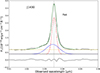
Same as Table 1 but for the Teacup and J1356S. In the case of J1356S, the tabulated flux for Brγ corresponds to 3σ upper limit, as the line is not detected there.
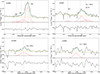
Appendix B: 3DBAROLO disc model
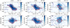 |
Fig. B.1. Same as Figure 7 but for the H2 stacked data cubes. The red and blue contours are drawn at (2, 3, 5)σ for J1430 and at (2, 3, 4)σ for J1356, where σ = 0.15 and σ = 0.21 for J1430 and J1356, respectively. |
In the following, we show the analog of the PVDs in Figure 7 but extracted from the stacked H2 cubes. The red contours refer to the 3DBAROLO models described in Section 4.3. Figures B.2 and B.3 show the channel maps produced by 3DBAROLO by fitting the H21-0S(1) data cubes of J1430 and J1356N. The color scale and the blue contours refer to the data, and the red contours correspond to 3DBAROLO disc model. The cyan cross indicates the peak of the emission and was chosen as the center of the model. The velocity of the channel map is reported above in each panel. We note that J1430 shows clumps of emission with velocities of up to ±480 km s−1, and J1356 up to ±370 km s−1.
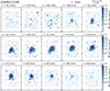 |
Fig. B.2. Channel maps of the H21-0S(1) emission line of J1430. Color scale maps and blue contours trace the emission in SINFONI data cube while red contours trace the emission in the 3DBAROLO model cube. Contours are drawn at (2, 4, 8, 16)σ. |
All Tables
Same as Table 1 but for the Teacup and J1356S. In the case of J1356S, the tabulated flux for Brγ corresponds to 3σ upper limit, as the line is not detected there.
All Figures
|
Fig. 1. Flux-calibrated nuclear spectra of the Teacup, J1356N and J1356S extracted in a circular aperture of 0.8″ diameter and smoothed using a 3 pixels boxcar. The most prominent emission lines are labeled. |
| In the text | |
|
Fig. 2. Line profiles showing the nuclear spectra of J1356N (top panels) and the Teacup (bottom panels), extracted in a circular aperture of 0.8″ diameter and smoothed using a 3 pixel boxcar. The corresponding fits are shown as solid green lines. Solid blue and dot-dashed red Gaussians are the broad- and narrow- line components, respectively, and the orange dashed line is the continuum. The Gaussians have been vertically shifted for displaying purposes. The insets at the bottom of each panel are the residuals. The gray dotted vertical lines mark the expected position of the line peaks according to the redshift of the QSO2s. |
| In the text | |
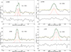 |
Fig. 3. Same as Figure 2 but for the H21-0S(1) and H21-0S(2) line profiles. |
| In the text | |
|
Fig. 4. Integrated intensity (i.e., moment 0) maps of the H21-0S(1), S(2), and stacked H2 of J1430 (top panels) and of J1356 (bottom panels). The black cross marks the peak of the near-infrared continuum. The maps have been smoothed using a two-spaxel boxcar for presentation purposes. Regions below 2σ are masked out. |
| In the text | |
|
Fig. 5. H21-0S(1) moment 1 and 2 maps (i.e., velocity and velocity dispersion) of the Teacup. The 3DBAROLO models of the moment 1 and 2 maps and the corresponding residuals are also shown. Regions below 2σ are masked out. The black cross mark the peak of the near-infrared continuum as in Figure 4. The kinematic major axis is shown as a black dashed line in the moment 1 maps. The PAjet = 60° is indicated as a black solid line and gray shaded area. The maps have been smoothed using a two-spaxel boxcar for presentation purposes. North is up and east to the left. |
| In the text | |
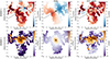 |
Fig. 6. Same as in Figure 5 but for J1356. |
| In the text | |
|
Fig. 7. PVDs extracted from the H21-0S(1) emission line data cubes. The blue contours trace the H21-0S(1) emission in SINFONI data cube, while the red contours trace the corresponding 3DBAROLO model. Left panels show the PVDs along the kinematic major (PA = 13°, top) and minor axis (PA = 103°, bottom) in J1430. Middle panels show the PVDs along (PA = 60°, top) and perpendicular (PA = 150°, bottom) to the radio jet direction in J1430. In the left and middle panels the blue and red contours are drawn at (2, 4, 8, 10)σ with σ = 3.23 10−19 W/m2/μm. Right panels: PVDs along the kinematic major (PA = 121°, top) and minor axis (PA = 211°, bottom) in J1356. The blue and red contours are drawn at (2, 3, 5)σ with σ = 3.26 10−19 W/m2/μm. All the PVDs were extracted using a slit of width 0.8″. |
| In the text | |
|
Fig. 8. Intensity maps of the high velocity components of the H21-0S(1) emission. The color map corresponds to the moment 0 of the total H21-0S(1) emission, while the contributions from high velocities are shown as red and blue contours. The spatial resolution of the SINFONI data is indicated with a gray ellipse in the bottom left corner. The white stars mark the peak of the near-infrared continuum as in Figure 4. Left panel: the red and blue contours of J1430 refer to velocities above ∼370 km s−1 with σred = 2.5 10−17 W/m2/μm.km s−1 and σblue = 2.7 10−17 W/m2/μm.km s−1. The red and blue contours are drawn at (2, 3,5, 7)σ. Right panel: the red contours of J1356 refer to velocities above ∼270 km s−1 with σred = 4.4 10−17 W/m2/μm.km s−1. The red contours are drawn at (2, 3, 4, 6)σ. |
| In the text | |
|
Fig. 9. Relative contribution of the cold molecular (turquoise), ionized (pink), and warm molecular (blue) phases to the total mass outflow rate. The blue labels refer to the relative contribution of the warm molecular phase in %. The galaxies whose names are in violet are the targets of this work. The ionized mass outflow rates are from SP24, adopting their [S II]-based electron densities and divided by us by a factor of 3 to match our outflow geometry. The cold molecular mass outflow rates are from Scenario II in Audibert et al. (2024), and the warm molecular mass outflow rate of J1509 is from Ramos Almeida et al. (2019). No warm molecular outfflow detections are yet reported for J1100. |
| In the text | |
|
Fig. B.1. Same as Figure 7 but for the H2 stacked data cubes. The red and blue contours are drawn at (2, 3, 5)σ for J1430 and at (2, 3, 4)σ for J1356, where σ = 0.15 and σ = 0.21 for J1430 and J1356, respectively. |
| In the text | |
|
Fig. B.2. Channel maps of the H21-0S(1) emission line of J1430. Color scale maps and blue contours trace the emission in SINFONI data cube while red contours trace the emission in the 3DBAROLO model cube. Contours are drawn at (2, 4, 8, 16)σ. |
| In the text | |
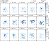 |
Fig. B.3. Same as Figure B.2 but for J1356. Contours are drawn at (2, 4, 8, 16)σ. |
| In the text | |
Current usage metrics show cumulative count of Article Views (full-text article views including HTML views, PDF and ePub downloads, according to the available data) and Abstracts Views on Vision4Press platform.
Data correspond to usage on the plateform after 2015. The current usage metrics is available 48-96 hours after online publication and is updated daily on week days.
Initial download of the metrics may take a while.