| Issue |
A&A
Volume 671, March 2023
|
|
|---|---|---|
| Article Number | L12 | |
| Number of page(s) | 9 | |
| Section | Letters to the Editor | |
| DOI | https://doi.org/10.1051/0004-6361/202345964 | |
| Published online | 21 March 2023 | |
Letter to the Editor
Jet-induced molecular gas excitation and turbulence in the Teacup
1
Instituto de Astrofísica de Canarias, Calle Vía Láctea, s/n, 38205 La Laguna, Tenerife, Spain
e-mail: This email address is being protected from spambots. You need JavaScript enabled to view it.
2
Departamento de Astrofísica, Universidad de La Laguna, 38206 La Laguna, Tenerife, Spain
3
Observatorio Astronómico Nacional (OAN-IGN)-Observatorio de Madrid, Alfonso XII, 3, 28014 Madrid, Spain
4
Observatoire de Paris, LERMA, Collège de France, PSL University, CNRS, Sorbonne University, Paris, France
5
Dipartimento di Fisica, Sezione di Astronomia, Universitá di Trieste, Via Tiepolo 11, 34143 Trieste, Italy
6
Inter-University Centre for Astronomy and Astrophysics, Savitribai Phule Pune University Campus, Pune 411007, India
7
Research School of Astronomy and Astrophysics, The Australian National University, Canberra, ACT 2611, Australia
8
Center for Computational Sciences, University of Tsukuba, Tennodai 1-1-1, 305-0006 Tsukuba, Ibaraki, Japan
Received:
20
January
2023
Accepted:
26
February
2023
Abstract
In order to investigate the impact of radio jets on the interstellar medium (ISM) of galaxies hosting active galactic nuclei (AGN), we present subarcsecond-resolution Atacama Large Millimeter/submillimeter Array (ALMA) CO(2-1) and CO(3-2) observations of the Teacup galaxy. This is a nearby (DL = 388 Mpc) radio-quiet type-2 quasar (QSO2) with a compact radio jet (Pjet ≈ 1043 erg s−1) that subtends a small angle from the molecular gas disc. Enhanced emission line widths perpendicular to the jet orientation have been reported for several nearby AGN for the ionised gas. For the molecular gas in the Teacup, not only do we find this enhancement in the velocity dispersion but also a higher brightness temperature ratio (T32/T21) perpendicular to the radio jet compared to the ratios found in the galaxy disc. Our results and the comparison with simulations suggest that the radio jet is compressing and accelerating the molecular gas, and driving a lateral outflow that shows enhanced velocity dispersion and higher gas excitation. These results provide further evidence that the coupling between the jet and the ISM is relevant to AGN feedback even in the case of radio-quiet galaxies.
Key words: galaxies: active / galaxies: individual: Teacup / galaxies: kinematics and dynamics / galaxies: jets / ISM: jets and outflows
© The Authors 2023
 Open Access article, published by EDP Sciences, under the terms of the Creative Commons Attribution License (https://creativecommons.org/licenses/by/4.0), which permits unrestricted use, distribution, and reproduction in any medium, provided the original work is properly cited.
This article is published in open access under the Subscribe to Open model. This email address is being protected from spambots. You need JavaScript enabled to view it. to support open access publication.
1. Introduction
The idea that outflows are almost ubiquitous in galaxies hosting active galactic nuclei (AGN) is supported by observational efforts in the past decades, as well as by the development of subgrid physics in cosmological models (Cielo et al. 2018; Nelson et al. 2019). The inclusion of AGN feedback in the recipes of simulations is necessary to explain the observed bright end of the galaxy luminosity function, as otherwise galaxies would grow too big and massive (Croton et al. 2006; Dubois et al. 2016).
One of the potential drivers of multi-phase outflows, even in the case of radio-quiet AGN, is the jets launched by the supermassive black hole (SMBH). These jets can strongly impact (sub)kiloparsec scales by altering the properties of the interstellar medium (ISM) of the host galaxies. Observational evidence for outflows driven by jets has been reported in ionised (e.g., Heckman et al. 1984; Jarvis et al. 2019; Cazzoli et al. 2022; Girdhar et al. 2022; Speranza et al. 2022) and molecular gas (e.g., Morganti et al. 2015; Oosterloo et al. 2019; García-Burillo et al. 2019; Murthy et al. 2022). Supporting the observational evidence, hydrodynamic simulations (Wagner & Bicknell 2011; Wagner et al. 2012; Mukherjee et. al 2018a) are able to reproduce the jet–ISM interaction and the impact of feedback induced by relativistic AGN jets inside the central kiloparsec of gas-rich radio galaxies. The models trace the evolution of a relativistic jet propagating in a two-phase ISM, gradually dispersing the clouds through the effect of the ram pressure and internal energy of the non-thermal plasma, and creating a cocoon of shocked material that drives multi-phase outflows as the bubble expands.
In recent work, Ramos Almeida et al. (2022, hereafter RA22) reported Atacama Large Millimeter/submillimeter Array (ALMA) CO(2-1) observations at ∼0 2 (400 pc) resolution of seven radio-quiet type-2 quasars (QSO2s; i.e., obscured quasars) at redshifts z ∼ 0.1, with bolometric luminosities of Lbol ≈ 1045 − 46 erg s−1. These QSO2s are part of the Quasar Feedback (http://research.iac.es/galeria/cra/qsofeed/) sample. Cold molecular outflows with intermediate properties between those of Seyfert galaxies and ultraluminous infrared galaxies (ULIRGs) were detected in the five QSO2s with CO(2-1) detections. Their molecular mass outflow rates are lower than those expected from their AGN luminosities (Fiore et al. 2017; Fluetsch et al. 2019), suggesting that other factors, such as the jet power, the spatial distribution of the dense gas, and the coupling between jets and the dense gas, might also be relevant.
Among the QSO2s studied in RA22, the Teacup (SDSS J143029.88+133912.0; J1430+1339) revealed a peculiar CO morphology and disturbed kinematics. This, in addition to the compact radio jet (extent of ∼0.8 kpc, PA = 60°) detected in Very Large Array (VLA) data at 0 25 resolution (Harrison et al. 2015), makes this object a promising target to study the jet–ISM interaction. The Teacup is hosted in a bulge-dominated galaxy showing signatures of a recent merger, including stellar shell-like features seen in the Hubble Space Telescope (HST) images (Keel et al. 2015). The nickname ‘Teacup’ stems from the 12 kpc ionised gas bubble (Keel et al. 2012) that is also detected in the radio with the VLA (Harrison et al. 2015), both shown in the left panel of Fig. 1. The [O III] kinematics reveal a ∼1 kpc scale nuclear outflow with maximum velocities of ∼−750 km s−1 (Villar Martín et al. 2014; Harrison et al. 2014). In the near infrared (NIR), blueshifted broad components with maximum velocities of −1100 km s−1 were measured from the Paα and [Si VI] emission lines, also extending ∼1 kpc and oriented at PA ∼ 70° (Ramos Almeida et al. 2017). The projected orientation and extension of the nuclear ionised outflow almost coincide with the compact jet, suggesting that the latter could be driving the outflow (Harrison et al. 2015). Therefore, the Teacup is one of the few nearby luminous AGN whose outflows have been characterised in different gas phases (ionised, warm, and cold molecular). This, together with its compact radio jet, makes it an ideal target to advance our understanding of how compact jets impact the multi-phase ISM of radio-quiet AGN.
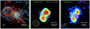 |
Fig. 1. Teacup as seen in [O III], radio continuum, and CO. The left panel shows the large-scale (15″×15″) [O III]λ5007 Å HST image in colour with the low-resolution VLA 6 GHz continuum contours overlaid in blue. The middle panel shows the 2 |


Here, we present new ALMA CO(3-2) observations at ∼0 6 (960 pc) resolution, in addition to the CO(2-1) 0
 2 data from RA22, to investigate the influence of the jet on the molecular gas excitation and kinematics of the Teacup. We adopt a flat ΛCDM cosmology with H0 = 70 km s−1 Mpc−1, ΩM = 0.3, and ΩΛ = 0.7.
2. Observations and data reduction
We present ALMA observations of the CO(2-1) and CO(3-2) emission lines observed in bands 6 and 7. The CO(2-1) observations and data reduction are described in detail in RA22. The CO(2-1) datacube has a synthesised beam size of 0 21×0
21×0 18 and a root mean square (rms) noise of 0.39 mJy beam−1 per channel of 10 km s−1. The CO(3-2) data (2016.1.01535.S; PI: G. Lansbury) were retrieved from the ALMA archive. The observations were made in April 2017 in the C40-3 configuration with an on-source integration time of 30.3 min and in a single pointing, covering a field of view (FoV) of 18″. The spectral window of 1.875 GHz total bandwidth was centred at the CO(3-2) line, with a channel spacing of 7.8 MHz, corresponding to ∼7.2 km s−1 after Hanning smoothing.
The CO(3-2) data were calibrated using the CASA software version 4.7.2 (McMullin et al. 2007) in the pipeline mode. The sources J1550+0527, J1337−1257 and J1446+1721 were used as flux, bandpass, and phase calibrators, respectively. Once calibrated, the imaging and cleaning were performed with the task TCLEAN. The spectral line map was obtained after subtracting the continuum in the uv-plane using the tasks UVCONTSUB and a zeroth-order polynomial in the channels free from emission lines. The CO(3-2) data cube was produced with a spectral resolution of 10 km s−1 (10.6 MHz) and using Briggs weighting mode and a robust parameter set to 0.5 in order to achieve the best compromise between resolution and sensitivity. Finally, the datacube was corrected for primary beam attenuation, resulting in a synthesised beam of 0 60×0
60×0 54 at PA = 59° and a rms noise of 1.9 mJy beam−1 per 10 km s−1 channel. In order to study the line ratios and compare the CO(2-1) to the new CO(3-2) datacube, we regridded the CO(2-1) data to the same pixel scale of the CO(3-2) and then convolved it to the same common beam size of 0
 60×0
60×0 54 (960 pc×860 pc).
The auxiliary radio data used here are the 6 GHz VLA observations of the Teacup in C-band in two different configurations: the high-resolution (0 25, HR) A-array and the low-resolution (1
 0, LR) B-array maps. The data were presented and analysed in full by Jarvis et al. (2019).
3. Results and analysis
The CO(3-2) peak intensity map shown in the middle panel of Fig. 1 shows the double-peaked morphology first detected in CO(2-1) and discussed in RA22. The distance between the two peaks is ∼0 8 (1.3 kpc). The integrated intensity, intensity-weighted velocity field, and velocity dispersion (σ) maps of the CO(3-2) emission are shown in Appendix A. Overall, the first- and second-moment maps (velocity field and σ) are similar to their CO(2-1) counterparts, although with a lower level of detail due to the coarser angular resolution. For example, the velocity field shows the disc-rotation pattern, but the disturbed kinematics seen in CO(2-1) are not detected in CO(3-2). The second-order moment map shows high values of σ, reaching ∼120 km s−1 with PA ∼ −30°, orthogonal to the radio jet orientation (PAjet = 60°), similar to the σ map of the CO(2-1) data in RA22.
In order to investigate the possible influence of the jet on the kinematics of the molecular gas, we created position-velocity diagrams (PVDs) along and perpendicular to the direction of the jet axis. We extracted them using a slit width of 0 6, equivalent the common resolution of the CO(3-2) and convolved CO(2-1) cubes. The PVDs are shown in Fig. 2 and the position and orientation of the slits are indicated as shaded rectangles in the left panel of Fig. 3. A broad gradient of velocities is detected both along and perpendicular to the jet axis, spanning up to ±400 km s−1 for both the CO(2-1) and CO(3-2) emission. We detect gas at higher velocities in the PVDs of CO(3-2) than in those of CO(2-1), especially in the case of the blueshifted velocities. The PVDs perpendicular to the radio jet show an inverted S-shape in the central ∼2″ (3.2 kpc), which includes the bulk of the emission. There is also a contribution from slow velocities (< 200 km s−1) at r > 1″ that resembles a rotation pattern, unlike the central part of the PVDs. These features were not reported in RA22 because of the narrower slit width and different orientations considered there.
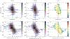 |
Fig. 2. PVDs along (PA = 60°) and perpendicular (PA = −30°) to the radio jet direction, extracted in a slit of 0 |

We analysed the CO(2-1) and CO(3-2) kinematics at 0 6 resolution using the ‘3D-Based Analysis of Rotating Objects from Line Observations’ (3DBAROLO) software by Di Teodoro & Fraternali (2015), following the methodology described in RA22. For the 3DFIT, we applied a mask using a threshold of 3σrms. We fixed the PA and the inclination of the disc to the values derived using the high-resolution CO(2-1) data in RA22: PAdisc = 4° and i = 38°, and the centre position was fixed to the continuum peak at 220 GHz (RA = 14h30m29.88s and Dec = +13d39m11.93s). Then, we allowed 3DBAROLO to fit the rotation velocity and velocity dispersion. From the model datacube created by 3DBAROLO, we produced PVDs extracted in slits with the same width and orientations described above, and overlaid them on the CO(2-1) and CO(3-2) PVDs (see red contours in Fig. 2). The bulk of the CO(2-1) and CO(3-2) emission at 0
 6 resolution can be well reproduced by our 3DBAROLO model. We find 77% and 90% of gas in rotation in CO(2-1) and CO(3-2), respectively, with a central velocity dispersion of ∼100 km s−1. For comparison, in the case of the CO(2-1) data at 0
 2 resolution, only 55% of the gas can be accounted for by rotation. This is because a significant fraction of non-circular and tangential motions are diluted because of the larger beam size of the CO(3-2) data. However, as shown in Fig. 2, the molecular gas with high velocities (∼±400 km s−1) cannot be explained by rotation, as the model reproduces the rotation pattern up to maximum values of around ±300 km s−1.
The right panels of Fig. 2 show the PVDs of the CO(3-2)/CO(2-1) line ratio. To produce these PVDs, the units of the CO(3-2) and CO(2-1) PVDs were first converted to brightness temperature (T32 and T21, in units of K), considering only CO emission above 2σrms. A clear increase in the line ratio is seen in regions of 0 4 radius (∼600 pc) along and perpendicular to the radio jet, up to values of 1.2. In order to study this line ratio in a spatially resolved manner, we created the T32/T21 line ratio of the integrated intensity (moment 0) maps, which is shown in the left panel of Fig. 3. This line ratio map shows the highest values, namely of ∼0.8, along the direction perpendicular to the radio jet, while other regions of the disc present ratios of 0.3 < T32/T21 < 0.5, similar to typical values found in settled discs or in the Milky Way (Leroy et al. 2009; Carilli & Walter 2013). We note that the values of T32/T21 in the integrated line-ratio map shown in Fig. 3 are lower than those in the PVDs shown in Fig. 2 because the former are average values along the line of sight (LOS). In the right panel of Fig. 3 we also show the σ map of the original CO(2-1) data (i.e., at 0
 2 resolution). The region with larger σ values (i.e., highest turbulence) coincides with that having the highest values of T32/T21. As discussed in Sect. 4, enhanced T32/T21 has been reported for a few nearby radio-loud AGN along the direction of the jet (e.g., Dasyra et al. 2016; Oosterloo et al. 2017, 2019), but to the best of our knowledge, this is the first detection of increased T32/T21 along the direction perpendicular to the radio jet in a radio-quiet AGN.
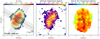 |
Fig. 3. Brightness temperature ratio (T32/T21) and CO(2-1) velocity dispersion maps. The left panel shows the T32/T21 map at 0 |


Using the 1.5 GHz VLA flux and the spectral index of α = −0.87 reported by Jarvis et al. (2019), it is possible to estimate the jet power of the Teacup from the relations of Bîrzan et al. (2008) and Cavagnolo et al. (2010), for example. If we do so, we obtain Pjet ≃ 1 − 3 × 1043 erg s−1. However, these scaling relations have large scatter (> 0.78 dex) and are drawn from samples of galaxies dominated by more evolved jets. Therefore, they may not apply to compact jets confined within the galaxy ISM, as is the case of the Teacup. As pointed out by Godfrey & Shabala (2016), the Pjet–Lradio relations may be unreliable because, among other things, they neglect the effect of distance, morphology, and environment. Here, we do not attempt to derive an accurate measurement of the jet power, but are only interested in its order of magnitude, as we aim to compare our findings with the simulations described in Sect. 4.2.
To perform this comparison, we also need an approximate estimate of the jet inclination relative to the CO disc. Although it is not possible to infer a precise angle using the radio data available, we obtain an estimate using the core-to-extended-radio-flux ratio parameter,  , where Score is the core flux density of the unresolved beamed nuclear jet, and Sext is the flux density of the unbeamed lobes. Statistically, Rc should be larger in more highly beamed objects, but the extended flux is time dependent and also depends on the frequency of observation. In the case of the Teacup, using the flux densities at 5.2 GHz reported by Jarvis et al. (2019) for the HR VLA data, we obtain Rc = (2.3/0.6) = 3.8, which would correspond to an angle of ∼20° relative to the LOS if we use Eq. (1) in Orr & Browne (1982) with γ = 5 and RT = 0.024. Considering the inclination of the CO disc derived from the modelling with 3DBAROLO (iCO = 38°; i.e. 52° relative to the LOS; RA22), we conclude that the jet likely subtends a small angle relative to the CO disc. The results presented here suggest that the radio jet is strongly coupled to the CO disc and because of that, it is driving turbulence and exciting the molecular gas along PA∼−30°.
4. Discussion
In this Letter we present robust observational evidence that the radio jet is interacting with the cold ISM of the Teacup and causing the disturbed kinematics, large turbulence, and peculiar excitation conditions of the gas. In the following, we discuss the results and compare them with high-resolution simulations of jets propagating in the ISM of galaxies.
4.1. Physical conditions and kinematics of the molecular gas
Spatially resolved CO emission-line ratio analyses have been reported for a few nearby Seyferts and radio galaxies. Viti et al. (2014) modelled the excitation conditions of the molecular gas in the circumnuclear disc of NGC 1068, and claimed that elevated values of R31 ≡ T32/T10 ∼ 5 (i.e., involving the CO(3-2) and CO(1-0) emission lines) and R21 ≡ T21/T10 ≳ 4 (involving CO(2-1) and CO(1-0) lines) correspond to hot dense gas (kinetic temperatures T > 150 K and η > 105 cm−3) excited by the AGN. Higher values of different emission-line ratios have been reported for the molecular gas interacting with the jet in the radio galaxy PKS 1549-79 (Oosterloo et al. 2019), and also in the Seyfert galaxy IC 5063 (Dasyra et al. 2016; Oosterloo et al. 2017). This indicates that jet-impacted regions have different gas-excitation conditions due to shocks and/or reduced optical thickness (Morganti et al. 2021). IC 5063 is a clear-cut example of jet coplanar with the galaxy disc, which is driving a multi-phase outflow (Tadhunter et al. 2014; Morganti et al. 2015). The jet power estimated for IC 5063 is Pjet ∼ 1044 erg s−1 and the PVD along the jet axis revealed T32/T21 values ranging from 1.0 to 1.5 in the outflowing regions, clearly different from the gas following regular rotation (R32 < 0.7). Under local thermodynamic equilibrium (LTE) conditions, R32 > 1 corresponds to excitation temperatures (Tex) of ∼50 K (Oosterloo et al. 2017). A similar temperature was found for the fast outflow gas component of IC 5063 using R42 ≡ T43/T21 > 1 (i.e., involving the CO(4-3) and CO(2-1) lines), suggesting that the gas in the outflow is optically thin (Dasyra et al. 2016).
The Teacup presents similar values of T32/T21 to those reported in the outflow region of IC 5063 (i.e., T32/T21 > 1; see Fig. 2). The difference is that in the Teacup, the highest values are found perpendicular and not along the jet direction, as shown in Fig. 3. This is indicative of the presence of hot dense gas, with Tex ∼ 50 K, probably excited by the cocoon of shocked gas that is driving the lateral outflow and/or turbulence that we observe in CO.
Regarding the gas kinematics, examples of enhanced σ of the ionised gas along the direction perpendicular to the jet axis have already been reported in the literature for nearby AGN. One example is the radio galaxy 3C 33, for which Couto et al. (2017) proposed a scenario in which the ISM is laterally expanding due to the passage of the jet, supported by the optical emission line ratios that they measured in the same region, which are typical of gas excitation induced by shocks. Venturi et al. (2021) reported high [O III] velocity widths in four nearby Seyfert galaxies from the MAGNUM survey hosting low-power radio jets. These high σ values were interpreted as being due to the passage of a low-inclination jet through the galaxy discs ISM, which produces shocks and induces turbulence. The MURALES survey of nearby 3CR radio sources revealed similar features in [O III] for some of the radio galaxies (Balmaverde et al. 2019, 2022). In the Teacup, we measure the highest values of the CO(2-1) and CO(3-2) σ perpendicular to the jet direction, namely of up to 140 km s−1. We note that the enhancement in T32/T21 is shifted by ∼0 2 to the east relative to the gas with the highest σ (see Figs. 3 and A.1). High-angular-resolution CO(3-2) observations are required in order to explore this shift in more detail.
4.2. Is the radio jet driving a lateral molecular outflow?
Simulations show that strong jet-induced feedback can occur even when Pjet ∼ 1043 − 44 erg s−1 (Mukherjee et al. 2016; Talbot et al. 2022). These low-power jets are trapped in the ISM of the galaxy for longer times and therefore they are able to disrupt the ISM over a larger volume than more powerful jets (Nyland et al. 2018). Another crucial element for having efficient feedback is the jet–ISM coupling. Simulations show that stronger coupling occurs when jets have low inclination relative to the gas disc, because jets are confined within the galaxy ISM, injecting more kinetic energy into the surrounding gas and inducing local turbulence and shocks (Mukherjee et al. 2018a; Meenakshi et al. 2022). According to the estimate described in Sect. 3, this seems to be the case for the Teacup.
We can compare the PVDs shown in Fig. 2 with simulation E in Meenakshi et al. (2022). This simulation consists of a jet of Pjet ∼ 1045 erg s−1 propagating in a gas disc with a central gas density of 200 cm−3, and subtending an angle of 20° (i.e., almost coplanar). This jet power is higher than our estimate for the Teacup (∼1043 erg s−1), but in addition to the caveats mentioned in Sect. 3, Pjet values estimated from the Bîrzan et al. (2008) and Cavagnolo et al. (2010) relations are usually lower limits for kpc-scale confined jets, such as in the case of the Teacup. For instance, in the case of IC 5063, the jet power required to model the jet-induced molecular gas dispersion was a factor of 3 to 10 higher than that inferred from scaling relations (Mukherjee et al. 2018b). The jet not only induces turbulence due to the injection of energy within its immediate vicinity but also causes a large broadening in the PVDs, with velocities reaching ∼400 km s−1 in the regions both along and perpendicular to the jet path (see Figs. 8 and 10 in Meenakshi et al. 2022).
Motivated by the resemblance between the ionised gas features in Sim E and the molecular gas features in the Teacup, we performed a comparison between our observations and the simulations in Meenakshi et al. (2022). Although the impact of jets on the dense molecular gas is not directly considered in the simulations, the emissivity of the CO(2-1) gas can be approximated with functions that depend on gas density, temperature, and cloud tracers, all extracted from the simulations. This method is similar to that adopted in Mukherjee et al. (2018b) to reproduce the molecular gas features observed in IC 5063. The details of the simulations are presented in Appendix B. As shown in the right panel of Fig. 3, the morphology of the gas velocity dispersion predicted by Sim E is similar to the Teacup, showing high values close to perpendicular to the jet direction. This happens because the main jet stream, as it propagates through the clumpy ISM, is split and deflected multiple times, carrying momentum in all directions including directions perpendicular to the jet axis and accelerating gas out of the disc plane. The simulated CO(2-1) PVDs along and perpendicular to the jet (see Fig. B.1) show high-velocity components reaching ±400 km s−1 within the central 2 kpc of the galaxy. Even though these simulations were not tailored to model the potential and radio power of the Teacup, they qualitatively reproduce the main kinematic features of the CO(3-2) and CO(2-1) observations.
4.3. Molecular outflow scenarios
Based on the CO(2-1) data at 0 2 resolution, RA22 reported evidence for a molecular outflow coplanar with the CO disc, with a velocity of 185 km s−1, radius of 0.5 kpc, and deprojected outflow rate of Ṁout = 15.8 M⊙ yr−1. This outflow rate is most likely a lower limit in the case of the Teacup because of the complex CO kinematics, and because RA22 only considered non-circular gas motions along the CO disc minor axis to compute the outflow mass. However, the PVDs along and perpendicular to the jet axis in Fig. 2 show high velocities, of up to ±400 km s−1, that cannot be reproduced with rotation, and both T32/T21 and σ (see Fig. 3) show higher values in the direction perpendicular to the jet (i.e., closer to the CO major axis). Therefore, it seems plausible that the higher gas excitation and increased turbulence that we find along PA = −30° are signatures of a jet-driven molecular outflow. We then considered different scenarios to compute the molecular outflow mass, which varies between 3×10⁷ and 6×10⁸ M⊙. The details are given in Appendix C.
Scenario I, the least conservative, consists of assuming that all the molecular gas that is not rotating, at least according to our 3DBAROLO model, is outflowing. Based on this model, we find that half of the molecular gas mass is rotating, and the outflow rate is 44 M⊙ yr−1 using an average outflow velocity of 100 km s−1. Scenario II assumes that only the high-velocity gas (faster than ±300 km s−1) participates in the outflow, and for this we measure 41 M⊙ yr−1. Finally, in Scenarios III and IV we measure outflow rates of 15.1 and 6.7 M⊙ yr−1 by subtracting the rotation curve from the CO(2-1) datacube and then considering high-velocity gas only (faster than ±300 km s−1 in Scenario III and just the high-velocity wings shown in Fig. C.2 in Scenario IV).
Based on the results presented in Sect. 3, aided by the simulations discussed in Sect. 4.2, we favour a scenario where the jet is pushing the molecular gas out of the disc plane and producing a lateral expansion that compresses the gas, increasing turbulence and gas excitation. Therefore, in principle we favour Scenarios II and III, which consider high-velocity gas only, without specifying any particular direction for the outflow. Considering this, the outflow mass would be in the range 5.6–16×107 M⊙, and the mass outflow rate within 15–41 M⊙ yr−1.
Jets produce efficient feedback by increasing the turbulence of the dense gas when the ratio between the radio power and the Eddington luminosity, Pjet/LEdd > 10−4 (Wagner et al. 2012). In the Teacup, this ratio is ∼9×10⁻⁴, and the jet power is sufficient to drive the molecular outflow because it is about two or three orders of magnitude higher than the outflow kinetic power (see Table C.1). However, the fate of the molecular gas during this feedback episode is a galactic fountain, because the escape velocity of the galaxy vesc ≳ 530 km s−1, estimated from its dynamical mass as in Feruglio et al. (2020), is larger than the fastest velocities in the outflow (∼±400 km s−1). Regardless, this will have a global effect on the evolution of the galaxy, redistributing mass, metals, and delaying further star formation.
Based on the results presented here, together with the predictions from the models described in Sect. 4.2, jet-induced turbulence and shocks are the most likely mechanisms to explain the high values of σ and T32/T21 reported here for the cold molecular gas in the Teacup. Larger samples of radio-quiet quasars showing low-power radio jets are required in order to better quantify the impact of jet–ISM coupling in the kinematics of the molecular gas.
Acknowledgments
We are grateful to the referee for very helpful and detailed comments. AA and CRA acknowledge the projects “Quantifying the impact of quasar feedback on galaxy evolution”, with reference EUR2020-112266, funded by MICINN-AEI/10.13039/501100011033 and the European Union NextGenerationEU/PRTR, and the Consejería de Economía, Conocimiento y Empleo del Gobierno de Canarias and the European Regional Development Fund (ERDF) under grant “Quasar feedback and molecular gas reservoirs”, with reference ProID2020010105, ACCISI/FEDER, UE. AA acknowledges funding from the MICINN (Spain) through the Juan de la Cierva-Formación program under contract FJC2020-046224-I. SGB acknowledges support from the research project PID2019-106027GA-C44 of the Spanish Ministerio de Ciencia e Innovación. This paper makes use of the following ALMA data: ADS/JAO.ALMA#2018.1.00870.S, and ADS/JAO.ALMA#2016.1.01535.S. ALMA is a partnership of ESO (representing its member states), NSF (USA) and NINS (Japan), together with NRC(Canada) and NSC and ASIAA (Taiwan), in cooperation with the Republic of Chile. The Joint ALMA Observatory is operated by ESO, AUI/NRAO and NAOJ. The National Radio Astronomy Observatory is a facility of the National Science Foundation operated under cooperative agreement by Associated Universities, Inc.
References
- Balmaverde, B., Capetti, A., Marconi, A., et al. 2019, A&A, 632, A124 [NASA ADS] [CrossRef] [EDP Sciences] [Google Scholar]
- Balmaverde, B., Capetti, A., Baldi, R. D., et al. 2022, A&A, 662, A23 [NASA ADS] [CrossRef] [EDP Sciences] [Google Scholar]
- Bîrzan, L., McNamara, B. R., Nulsen, P. E. J., Carilli, C. L., & Wise, M. W. 2008, ApJ, 686, 859 [Google Scholar]
- Carilli, C. L., & Walter, F. 2013, ARA&A, 51, 105 [NASA ADS] [CrossRef] [Google Scholar]
- Cavagnolo, K. W., McNamara, B. R., Nulsen, P. E. J., et al. 2010, ApJ, 720, 1066 [Google Scholar]
- Cazzoli, S., Hermosa Muñoz, L., Márquez, I., et al. 2022, A&A, 664, A135 [NASA ADS] [CrossRef] [EDP Sciences] [Google Scholar]
- Cielo, S., Bieri, R., Volonteri, M., Wagner, A. Y., & Dubois, Y. 2018, MNRAS, 477, 1336 [NASA ADS] [CrossRef] [Google Scholar]
- Couto, G. S., Storchi-Bergmann, T., & Schnorr-Müller, A. 2017, MNRAS, 469, 1573 [NASA ADS] [CrossRef] [Google Scholar]
- Croton, D. J., Springel, V., White, S. D. M., et al. 2006, MNRAS, 365, 11 [Google Scholar]
- Dasyra, K. M., Combes, F., Oosterloo, T., et al. 2016, A&A, 595, L7 [NASA ADS] [CrossRef] [EDP Sciences] [Google Scholar]
- Di Teodoro, E. M., & Fraternali, F. 2015, MNRAS, 451, 3021 [Google Scholar]
- Downes, D., & Solomon, P. M. 1998, ApJ, 507, 615 [NASA ADS] [CrossRef] [Google Scholar]
- Dubois, Y., Peirani, S., Pichon, C., et al. 2016, MNRAS, 463, 3948 [Google Scholar]
- Feruglio, C., Fabbiano, G., Bischetti, M., et al. 2020, ApJ, 890, 29 [Google Scholar]
- Fiore, F., Feruglio, C., Shankar, F., et al. 2017, A&A, 601, A143 [NASA ADS] [CrossRef] [EDP Sciences] [Google Scholar]
- Fluetsch, A., Maiolino, R., Carniani, S., et al. 2019, MNRAS, 483, 4586 [NASA ADS] [Google Scholar]
- García-Burillo, S., Combes, F., Ramos Almeida, C., et al. 2019, A&A, 632, A61 [Google Scholar]
- Girdhar, A., Harrison, C. M., Mainieri, V., et al. 2022, MNRAS, 512, 1608 [NASA ADS] [CrossRef] [Google Scholar]
- Godfrey, L. E. H., & Shabala, S. S. 2016, MNRAS, 456, 1172 [NASA ADS] [CrossRef] [Google Scholar]
- Harrison, C. M., Alexander, D. M., Mullaney, J. R., & Swinbank, A. M. 2014, MNRAS, 441, 3306 [Google Scholar]
- Harrison, C. M., Thomson, A. P., Alexander, D. M., et al. 2015, ApJ, 800, 45 [Google Scholar]
- Heckman, T. M., van Breugel, W. J. M., & Miley, G. K. 1984, ApJ, 286, 509 [NASA ADS] [CrossRef] [Google Scholar]
- Jarvis, M. E., Harrison, C. M., Thomson, A. P., et al. 2019, MNRAS, 485, 2710 [Google Scholar]
- Keel, W. C., Chojnowski, S. D., Bennert, V. N., et al. 2012, MNRAS, 420, 878 [Google Scholar]
- Keel, W. C., Maksym, W. P., Bennert, V. N., et al. 2015, AJ, 149, 155 [NASA ADS] [CrossRef] [Google Scholar]
- Leroy, A. K., Walter, F., Bigiel, F., et al. 2009, AJ, 137, 4670 [Google Scholar]
- McMullin, J. P., Waters, B., Schiebel, D., Young, W., & Golap, K. 2007, in Astronomical Data Analysis Software and Systems XVI, eds. R. A. Shaw, F. Hill, & D. J. Bell, ASP Conf. Ser., 376, 127 [Google Scholar]
- Meenakshi, M., Mukherjee, D., Wagner, A. Y., et al. 2022, MNRAS, 516, 766 [NASA ADS] [CrossRef] [Google Scholar]
- Morganti, R., Oosterloo, T., Oonk, J. B. R., Frieswijk, W., & Tadhunter, C. 2015, A&A, 580, A1 [NASA ADS] [CrossRef] [EDP Sciences] [Google Scholar]
- Morganti, R., Oosterloo, T., Murthy, S., & Tadhunter, C. 2021, Astron. Nachr., 342, 1135 [NASA ADS] [CrossRef] [Google Scholar]
- Mukherjee, D., Bicknell, G. V., Sutherland, R., & Wagner, A. 2016, MNRAS, 461, 967 [NASA ADS] [CrossRef] [Google Scholar]
- Mukherjee, D., Bicknell, G. V., Wagner, A. Y., Sutherland, R. S., & Silk, J. 2018a, MNRAS, 479, 5544 [NASA ADS] [CrossRef] [Google Scholar]
- Mukherjee, D., Wagner, A. Y., Bicknell, G. V., et al. 2018b, MNRAS, 476, 80 [NASA ADS] [CrossRef] [Google Scholar]
- Murthy, S., Morganti, R., Wagner, A. Y., et al. 2022, Nat. Astron., 6, 488 [CrossRef] [Google Scholar]
- Nelson, D., Pillepich, A., Springel, V., et al. 2019, MNRAS, 490, 3234 [Google Scholar]
- Nyland, K., Harwood, J. J., Mukherjee, D., et al. 2018, ApJ, 859, 23 [NASA ADS] [CrossRef] [Google Scholar]
- Oosterloo, T., Raymond Oonk, J. B., Morganti, R., et al. 2017, A&A, 608, A38 [NASA ADS] [CrossRef] [EDP Sciences] [Google Scholar]
- Oosterloo, T., Morganti, R., Tadhunter, C., et al. 2019, A&A, 632, A66 [NASA ADS] [CrossRef] [EDP Sciences] [Google Scholar]
- Orr, M. J. L., & Browne, I. W. A. 1982, MNRAS, 200, 1067 [CrossRef] [Google Scholar]
- Ramos Almeida, C., Piqueras López, J., Villar-Martín, M., & Bessiere, P. S. 2017, MNRAS, 470, 964 [NASA ADS] [CrossRef] [Google Scholar]
- Ramos Almeida, C., Bischetti, M., García-Burillo, S., et al. 2022, A&A, 658, A155 [NASA ADS] [CrossRef] [EDP Sciences] [Google Scholar]
- Rupke, D. S., Veilleux, S., & Sanders, D. B. 2005, ApJS, 160, 115 [Google Scholar]
- Solomon, P. M., & Vanden Bout, P. A. 2005, ARA&A, 43, 677 [NASA ADS] [CrossRef] [Google Scholar]
- Speranza, G., Ramos Almeida, C., Acosta-Pulido, J. A., et al. 2022, A&A, 665, A55 [NASA ADS] [CrossRef] [EDP Sciences] [Google Scholar]
- Tadhunter, C., Morganti, R., Rose, M., Oonk, J. B. R., & Oosterloo, T. 2014, Nature, 511, 440 [Google Scholar]
- Talbot, R. Y., Sijacki, D., & Bourne, M. A. 2022, MNRAS, 514, 4535 [NASA ADS] [CrossRef] [Google Scholar]
- Venturi, G., Cresci, G., Marconi, A., et al. 2021, A&A, 648, A17 [NASA ADS] [CrossRef] [EDP Sciences] [Google Scholar]
- Villar Martín, M., Emonts, B., Humphrey, A., Cabrera Lavers, A., & Binette, L. 2014, MNRAS, 440, 3202 [CrossRef] [Google Scholar]
- Viti, S., García-Burillo, S., Fuente, A., et al. 2014, A&A, 570, A28 [NASA ADS] [CrossRef] [EDP Sciences] [Google Scholar]
- Wagner, A. Y., & Bicknell, G. V. 2011, ApJ, 728, 29 [NASA ADS] [CrossRef] [Google Scholar]
- Wagner, A. Y., Bicknell, G. V., & Umemura, M. 2012, ApJ, 757, 136 [CrossRef] [Google Scholar]
Appendix A: Moment maps of the CO(3-2) emission
We computed the moment maps of the CO(3-2) emission at ∼0 6 resolution as described in Section 3. The integrated intensity, intensity-weighted velocity field, and velocity dispersion maps (moments 0, 1, and 2) are shown in Figure A.1.
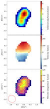 |
Fig. A.1. Moment maps of the CO(3-2) emission of the Teacup. Top, middle, and bottom panels correspond to the integrated intensity (moment 0, in Jy beam−1 km s−1 units), intensity weighted velocity field (moment 1, in km s−1), and σ (moment 2, in km s−1), respectively. East is to the left and north to the top. In the σ map, the contours show the T32/T21 of Figure 3 at 0.5, 0.6, and 0.7, and the red ellipse in the bottom left corner indicates the beam size. |
Appendix B: Simulation of jet propagating in the molecular disc
In order to elucidate the nature of the jet–ISM interaction in the Teacup, we present here qualitative comparisons with the kinematics of the dense gas in simulations D and E of Mukherjee et al. (2018a, hereafter Sim D and E) using the diagnostics developed in Meenakshi et al. (2022). In these simulations, jets of power 1045 erg s−1 are launched at angles of 45° and 20° from the disc plane for Sim D and E respectively. These inclinations resemble the angle subtended by the jet and the CO disc in the Teacup. It should be noted that although the simulations are not tailored to mimic the Teacup, we performed a qualitative comparison to try to understand the jet–gas interaction in this galaxy, as in Murthy et al. (2022).
In these simulations, a turbulent dense gas disc of radius ∼2 kpc is placed in the X − Y plane. A pair of relativistic jets are launched from the centre. The jet’s axis lies in the X − Z plane, inclined from the disc at different angles of choice. According to the simulation’s conventions, θI = 90°, ΦI = 360° corresponds to the edge-on view, with the observer facing the X − Z plane. For the analysis below, we have used the value θI = 52° to match that of the Teacup. The azimuthal angle ϕI is varied to match the observed relative orientation of the projected jet’s axis to the disc. The image plane is inverted to the observed orientation of Teacup to facilitate the visual comparison of the simulated maps.
For the analysis, we constructed mean LOS velocities, and the PVDs weighted by synthetic CO luminosities, following the method outlined in Section 5.2 of Mukherjee et al. (2018b) and adopting the same parameters as in their work. Dense gas regions with temperatures lower than 5000 K and densities higher than 10 cm−3 were used for this analysis. The PVDs are then produced using slits of 500 pc in width oriented along and perpendicular to the jet. In Figure B.1, the top left panel shows the projected velocity map for Sim E at a θI = 52° and ϕI = 340°, overlaid by the jet tracer at a value of 0.05. At this orientation, the jet subtends an angle of 25° from the LOS. The PVDs along and perpendicular to the jet are shown in the top right panels. The jet induces high velocities along both slits, reaching values of up to ∼±400 km s−1, and with the largest dispersion appearing in the central 1 kpc regions. The morphology of the PVD for the perpendicular slit is also very similar to that obtained for the Teacup in Figure 2, which appears to be sharply curved due to contribution from the rotation pattern of the disc. In the bottom panels of Fig. B.1, we show the mean velocity field and PVDs for Sim D, which are produced for an image plane oriented at θI = 52° and ϕI = 30°. This corresponds to an angle of 23.5° between the jet and the LOS. Similar to Sim E, the PVDs along and perpendicular to the jet in Figure B.1 also exhibit velocities of up to ∼±400 km s−1 within the central 2 kpc.
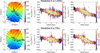 |
Fig. B.1. Snapshots of the mean velocity field and PVDs from Sim E (top panels, jet inclined 20° relative to the disc) and Sim D (bottom panels, jet inclined at 45°) for Pjet = 1045 erg s−1 at 1.24 Myr and 1 Myr, respectively. Left panels: Mean LOS velocity fields with the position of the slits of 500 pc width along (dashed lines) and perpendicular (solid lines) to the jet. Middle and right panels: PVDs along and perpendicular to the jet. The green curves are the mean velocity curve with ±2σ deviation, with a maximum deviations along and perpendicular to the jet reaching 408 (448) km s−1 and 434 (412) km s−1, respectively, for Sim E (Sim D). |
The simulated σ maps at the resolution of 100 pc and smoothed in the 2D domain by convolving with a Gaussian of similar kernel width are shown in Figure B.2. The σ distribution from Sim E (top panels) displays the highest values along the direction perpendicular to the jet path, similar to the observed spatial distribution of σ, shown in Figure 3. The σ map from Sim D (see bottom panels of Fig. B.2) also shows high values in the regions perpendicular to jet, although more compact than in Sim E, with the highest values along the jet. This extended velocity dispersion is caused by the jet-driven outflows along the minor axis, as well as along other directions throughout the disc, with the former being more prominent (e.g. see Figs. 7 and 8 in Meenakshi et al. 2022). This indicates that the jet–gas interaction in the nuclear regions of the disc can lead to high-velocity dispersion in the molecular gas distribution that can extend in directions perpendicular to the jet. Such an enhanced dispersion can arise both from direct uplifting of the gas from the disc in the form of outflows (e.g. see Fig. 14 of Meenakshi et al. 2022), as well as turbulence introduced into the gas disc by the jet-driven bubble.
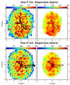 |
Fig. B.2. σ maps from Sim E (top panels) and D (bottom panels). Left panels: Maps at a resolution of 100 pc. Right panels: Simulated maps and jet-tracer smoothed by convolving with a 2D Gaussian of width 100 pc and 60 pc, respectively. The jet tracer is shown at 0.05 contour level. |
Appendix C: Outflow scenarios
Here we describe the four scenarios that we considered for estimating the outflow masses and mass rates, from the least to the most conservative. For this analysis, we only used the CO(2-1) data at the original 0 2 resolution to avoid artefacts or incorrect interpretations of the results due to beam smearing of the larger CO(3-2) beam size.
I) In the first scenario, we assume that all the molecular gas that cannot be reproduced with our rotating disc model is outflowing. Thus, we simply integrated the emission the 3DBAROLO model and subtracted it from the CO(2-1) datacube. We find that only 55% of the CO(2-1) emission can be reproduced with rotation, and the remaining 45% would correspond to an outflow mass of 5.1×10⁸ M⊙. However, as mentioned in Section 3, the PVDs perpendicular to the jet (PA=-30°; bottom panels in Figure 2) show an inverted S-shape in the central r∼1″ (1.6 kpc), which includes the bulk of the emission, and also low-velocity extended emission at r> 1″ that is only detected at 2σrms. Thus, there is some extended low-velocity gas that is not accounted for by our rotating model, and some nuclear high-velocity gas that is considered by 3DBAROLO as rotation while it might not be. This uncertainty is not considered in the errors listed in Table C.1. In this scenario, we adopted an outflow velocity of vout = 100 km s−1, estimated from the mean velocity residuals from the 3DBAROLO fit in blue RA22.
II) In the second scenario, we consider that only the highest velocities, faster than ±300 km s−1, correspond to outflowing gas. We chose this value from the comparison of the PVDs shown in Figure 2 and the 3DBAROLO rotation curve, shown in red the same figure. To calculate the flux of the high velocity gas, we created moment 0 maps by selecting only channels above ±300 km s−1, shown in Figure C.1. In this scenario, the mass corresponding to the outflow is 1.6×10⁸ M⊙.
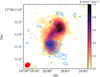 |
Fig. C.1. Integrated intensity of the high-velocity components of the CO(2-1) emission at 0 |


Outflow measurements for the four scenarios proposed for the Teacup.
III) The third scenario is amalgam of scenarios I and II. We assume that all the high-velocity gas is outflowing, but the contribution from rotation is subtracted following a similar approach as in García-Burillo et al. (2019). We deprojected the one-dimensional rotation curve to the corresponding velocity field on a pixel-by-pixel basis, and reshuffled the channels in order to remove the rotation component from the velocity axis of the CO(2-1) datacube. The result is a narrow residual CO profile, i.e. without the rotation component, which is shown in Figure C.2. As this method is suited to optimising the signal-to-noise ratio of the emission associated with non-circular motions, it can reveal high-velocity wings that are otherwise too faint to be detected. Using the residual profile and considering only gas with velocities above ±300 km s−1, we derive a mass of 5.7×10⁷ M⊙ for the outflow.
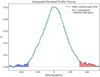 |
Fig. C.2. Integrated CO(2-1) residual profile after subtraction of the rotation curve. High-velocity blue and red wings are detected after subtraction. The cyan solid line corresponds to the fit with a single Gaussian component of FWHM∼330 km s−1 used in Scenario IV. The blue and red shaded areas correspond to the high-velocity gas considered to compute the outflow flux in Scenario III. |
IV) The fourth scenario is based on the method described in scenario III, but it assumes that the bulk of the residual CO profile shown in Figure C.2 corresponds to turbulence unrelated to the outflow. This turbulence can be due to the merger, or produced by the jet, but here we consider that it does not correspond to outflowing gas. The residual profile can be fitted with a single Gaussian of FWHM∼330 km s−1, as shown in Figure C.2. If we subtract this Gaussian from the total residual profile, we measure a mass of 2.6×10⁷ M⊙, which mainly corresponds to the high-velocity wings.
We computed the outflow masses from the integrated flux measurements in the outflow. First, the integrated fluxes are converted to CO luminosities  , in units of K km s−1 pc2 using Equation 3 of Solomon & Vanden Bout (2005) and then translated into masses using the CO-to-H2 (αCO) conversion factor
  . Under the assumption that the gas is thermalised and optically thick, the brightness temperature ratio
  . A conservative α = 0.8 is usually adopted for deriving outflow masses (see blue RA22 and references therein). The values for each scenario are listed in Table C.1.
To compute mass outflow rates, we use an outflow radius of rout = 0 75 (1.2 kpc), as constrained from the extent of the high-velocity gas with high σ and T32/T21 (see Figures 2 and 3). The outflow velocities reach up to ±400 km s−1, but here we adopt a more conservative velocity of vout = 300 km s−1, except for Scenario I. For a time-averaged, thin, expelled shell geometry (Rupke et al. 2005), Ṁout = vout(Mout/rout), which corresponds to the outflow mass averaged over the flow timescale, tflow = Rout/vout = 3.9 Myr. Considering all the previous, the mass outflow rates are in the range Ṁout = 6.7−44 M⊙ yr−1. The ratio between the kinetic power of the molecular outflow (
 ) and the jet power varies from 0.004 < Ėkin/Pjet < 0.035 (see Table C.1), indicating that the jet has sufficient kinetic energy to drive the molecular outflow.
All Tables
All Figures
|
Fig. 1. Teacup as seen in [O III], radio continuum, and CO. The left panel shows the large-scale (15″×15″) [O III]λ5007 Å HST image in colour with the low-resolution VLA 6 GHz continuum contours overlaid in blue. The middle panel shows the 2 |
| In the text | |
|
Fig. 2. PVDs along (PA = 60°) and perpendicular (PA = −30°) to the radio jet direction, extracted in a slit of 0 |
| In the text | |
|
Fig. 3. Brightness temperature ratio (T32/T21) and CO(2-1) velocity dispersion maps. The left panel shows the T32/T21 map at 0 |
| In the text | |
|
Fig. A.1. Moment maps of the CO(3-2) emission of the Teacup. Top, middle, and bottom panels correspond to the integrated intensity (moment 0, in Jy beam−1 km s−1 units), intensity weighted velocity field (moment 1, in km s−1), and σ (moment 2, in km s−1), respectively. East is to the left and north to the top. In the σ map, the contours show the T32/T21 of Figure 3 at 0.5, 0.6, and 0.7, and the red ellipse in the bottom left corner indicates the beam size. |
| In the text | |
|
Fig. B.1. Snapshots of the mean velocity field and PVDs from Sim E (top panels, jet inclined 20° relative to the disc) and Sim D (bottom panels, jet inclined at 45°) for Pjet = 1045 erg s−1 at 1.24 Myr and 1 Myr, respectively. Left panels: Mean LOS velocity fields with the position of the slits of 500 pc width along (dashed lines) and perpendicular (solid lines) to the jet. Middle and right panels: PVDs along and perpendicular to the jet. The green curves are the mean velocity curve with ±2σ deviation, with a maximum deviations along and perpendicular to the jet reaching 408 (448) km s−1 and 434 (412) km s−1, respectively, for Sim E (Sim D). |
| In the text | |
|
Fig. B.2. σ maps from Sim E (top panels) and D (bottom panels). Left panels: Maps at a resolution of 100 pc. Right panels: Simulated maps and jet-tracer smoothed by convolving with a 2D Gaussian of width 100 pc and 60 pc, respectively. The jet tracer is shown at 0.05 contour level. |
| In the text | |
|
Fig. C.1. Integrated intensity of the high-velocity components of the CO(2-1) emission at 0 |
| In the text | |
|
Fig. C.2. Integrated CO(2-1) residual profile after subtraction of the rotation curve. High-velocity blue and red wings are detected after subtraction. The cyan solid line corresponds to the fit with a single Gaussian component of FWHM∼330 km s−1 used in Scenario IV. The blue and red shaded areas correspond to the high-velocity gas considered to compute the outflow flux in Scenario III. |
| In the text | |
Current usage metrics show cumulative count of Article Views (full-text article views including HTML views, PDF and ePub downloads, according to the available data) and Abstracts Views on Vision4Press platform.
Data correspond to usage on the plateform after 2015. The current usage metrics is available 48-96 hours after online publication and is updated daily on week days.
Initial download of the metrics may take a while.