| Issue |
A&A
Volume 696, April 2025
|
|
|---|---|---|
| Article Number | A243 | |
| Number of page(s) | 24 | |
| Section | Catalogs and data | |
| DOI | https://doi.org/10.1051/0004-6361/202348735 | |
| Published online | 30 April 2025 | |
Kepler meets Gaia DR3: Homogeneous extinction-corrected color-magnitude diagram and binary classification
1
Instituto de Astrofísica de Canarias (IAC),
38205
La Laguna, Tenerife,
Spain
2
Universidad de La Laguna (ULL), Departamento de Astrofísica,
38206
La Laguna, Tenerife,
Spain
3
Université Paris-Saclay, Université Paris Cité, CEA, CNRS, AIM,
91191
Gif-sur-Yvette,
France
4
Department of Astronomy, The Ohio State University,
140 West 18th Avenue,
Columbus,
OH
43210,
USA
5
Instituto de Astrofísica e Ciências do Espaço, Universidade do Porto, CAUP, Rua das Estrelas,
PT4150-762
Porto,
Portugal
6
Institut für Physik, Karl-Franzens Universität Graz,
Universitätsplatz 5/II, NAWI Graz,
8010
Graz,
Austria
7
Sydney Institute for Astronomy (SIfA), School of Physics, University of Sydney,
NSW 2006,
Australia
8
Center for Computational Astrophysics, Flatiron Institute,
162 5th Avenue,
Manhattan,
NY,
USA
9
Astronomical Institute, Faculty of Mathematics and Physics, Charles University,
V Holešovičkách 2,
180000
Prague,
Czech Republic
★ Corresponding author: This email address is being protected from spambots. You need JavaScript enabled to view it.
Received:
25
November
2023
Accepted:
26
January
2025
Abstract
The original Kepler mission has delivered unprecedented high-quality photometry. These data have impacted numerous research fields (e.g., asteroseismology and exoplanets), and continue to be an astrophysical goldmine. Because of this, thorough investigations of the ~200 000 stars observed by Kepler remain of paramount importance. In this paper, we present a state-of-the-art characterization of the Kepler targets based on Gaia DR3 data. We placed the stars on the color-magnitude diagram (CMD), accounted for the effects of interstellar extinction, and classified targets into several CMD categories (dwarfs, subgiants, red giants, photometric binaries, and others). Additionally, we report various categories of candidate binary systems spanning a range of detection methods, such as renormalised unit weight error, radial velocity variables, Gaia non-single stars, Kepler and Gaia eclipsing binaries from the literature, among others. First and foremost, our work can assist in the selection of stellar and exoplanet host samples regarding CMD and binary populations. We further complemented our catalog by quantifying the impact that astrometric differences between Gaia data releases have on CMD location, assessing the contamination in asteroseismic targets with properties at odds with Gaia, and identifying stars flagged as photometrically variable by Gaia. We make our catalog publicly available as a resource to the community when researching the stars observed by Kepler.
Key words: methods: data analysis / catalogs / binaries: general / stars: evolution / Hertzsprung-Russell and C-M diagrams / stars: variables: general
© The Authors 2025
 Open Access article, published by EDP Sciences, under the terms of the Creative Commons Attribution License (https://creativecommons.org/licenses/by/4.0), which permits unrestricted use, distribution, and reproduction in any medium, provided the original work is properly cited.
This article is published in open access under the Subscribe to Open model. This email address is being protected from spambots. You need JavaScript enabled to view it. to support open access publication.
1 Introduction
Since its launch 15 years ago, the Kepler space telescope (Borucki et al. 2010) has deeply revolutionized astrophysics. The impact of its high-precision photometry has allowed unprecedented discoveries, with contributions spanning the fields of asteroseismology, stellar rotation, stellar activity, exoplanets, and Galactic archaeology, among others (e.g., Bedding et al. 2011; Beck et al. 2012; Howard et al. 2012; Mosser et al. 2012; Miglio et al. 2013; Batalha et al. 2013; McQuillan et al. 2014; van Saders et al. 2016; Silva Aguirre et al. 2017). Although the mission was retired in 2018, after being refurbished into K2 for the second part of its life (Howell et al. 2014), the community is still analyzing its data and producing novel scientific studies (e.g., Santos et al. 2021, 2023; Li et al. 2022; Mathur et al. 2022, 2023; Vrard et al. 2022; Long et al. 2023; Martínez-Palomera et al. 2023; Reinhold et al. 2023; Bhalotia et al. 2024; Kamai & Perets 2025). Hence, detailed characterizations of the stars observed by Kepler remain highly relevant.
In this context, the Gaia mission (Gaia Collaboration 2016, 2018b) has provided exquisite all-sky data that allow for unprecedented characterizations of stars (e.g., Berger et al. 2018; Brandt 2018; Cantat-Gaudin et al. 2018; Godoy-Rivera et al. 2021b; Kuhn et al. 2019). The Early Data Release 3 (EDR3) reports the latest astrometric and photometric data (Gaia Collaboration 2021; Lindegren et al. 2021b; Riello et al. 2021), and the more recent DR3 delivers several lists of binary systems, as well as radial velocity measurements, extinction values, and other stellar parameters (Gaia Collaboration 2023d,b; Creevey et al. 2023; Fouesneau et al. 2023; Halbwachs et al. 2023; Katz et al. 2023).
The goal of this paper is to leverage the latest Gaia data and perform a thorough characterization of the Kepler stars, specifically regarding target selections of singles vs. binaries and main sequence (MS) vs. post-MS phases. For instance, when focused on single stars, removing stars with binary companions is relevant as they may pollute the signal or influence the evolution given their proximity (Curtis et al. 2019; Lu et al. 2022; Santos et al. 2024). Conversely, studies dedicated to binary stars require a comprehensive selection of these systems, spanning a range of properties and detection methods (Gaulme et al. 2016; Ball et al. 2023; Grossmann et al. 2025). Similarly, post-MS evolution can produce variations in stellar properties driven by the structural changes experienced by stars (García et al. 2014; Santos et al. 2019; Hall et al. 2021; Gehan et al. 2024). Some of the analyses that would benefit from such a characterization regarding Kepler include the aforementioned fields of stellar, exoplanetary, and Galactic astrophysics.
This paper is structured as follows. In Sect. 2 we present the Kepler sample and the Gaia data we used to characterize it. In Sect. 3 we investigate the color-magnitude diagram (CMD) and separate the sample into different CMD categories. In Sect. 4 we use a variety of detection methods to identify several categories of binary systems. In Sect. 5 we study the impact that revised DR3 distances have on CMD location. In Sect. 6 we illustrate how the Gaia data can shed light on puzzling asteroseismic targets. In Sect. 7 we examine the Gaia variability classification on the Kepler targets. We conclude in Sect. 8.
2 Data
We defined the target sample as the stars observed by the Kepler mission reported in the one-to-one Gaia-Kepler.fun1 crossmatch. This amounted to a list of 196 762 stars with Kepler Input Catalog (KIC) identifiers (hereafter KIC IDs; Brown et al. 2011) that also have Gaia DR3 IDs.
Given the much higher angular resolution of the Gaia mission compared to Kepler, for some stars the crossmatching may not be straightforward (e.g., a given Kepler target may be matched to more than one Gaia source). For this work, we focused on the one-to-one match table, i.e., the subset of Kepler targets that can be confidently matched to exactly one Gaia ID and vice versa. We noted that this crossmatch was conservative to some extent, as for a given Kepler star, it was calculated by enforcing three conditions: (1) that within 4″, the nearest Gaia match in angular separation was also the nearest match by magnitude difference between Gaia G and Kepler Kp; (2) that the angular separation was less than 1″ after proper motion correction; and (3) that the G and Kp brightnesses were within 2 magnitudes.
While not fully complete, this crossmatch included the vast majority of the stars observed by Kepler. For instance, our target sample included 99.1% (195 288 out of 197 096 stars) of the Kepler DR25 catalog by Mathur et al. (2017). We leave the remaining 0.9% (1808 stars) to be further examined in future studies.
Using these Gaia DR3 IDs, we obtained the Gaia magnitudes, parallaxes, and renormalised unit weight error (RUWE) values by querying the gaiadr3.gaia_source table. We corrected the parallaxes by subtracting the zero-point values2 from Lindegren et al. (2021a,b), and the parallax errors by considering the inflation factors from El-Badry et al. (2021). We calculated distances by inverting the (corrected) parallax values. Given the quality cuts we introduce in Sect. 3, the parallax inverse is a safe estimate for our targets (Bailer-Jones et al. 2021). To confirm this we queried the gaiaedr3_distance table from Bailer-Jones et al. (2021) and found that our distances agree well with their geometric distances (e.g., both estimates agreed at the 95% level or better for 97.4% of cases). Additionally, we queried the gaiadr3.astrophysical_parameters table for spectroscopic metallicities ([M/H]), surface gravities (log(g)), and effective temperatures (Teff). We found 12.1% of the sample (23 894 stars) prior to any quality cuts. We discuss the calibrations applied to the [M/H] and log(g) values, as well as the selection of targets with high-quality spectroscopic parameters, in Appendix B.
In Table A.1, we report the KIC IDs, Gaia DR3 IDs, and main astrometric, photometric, and spectroscopic Gaia DR3 data for the sample. To further enhance the value of our catalog, in Table A.1 we also include the TESS Input Catalog (TIC; Stassun et al. 2018, 2019) and Two Micron All Sky Survey (2MASS; Cutri et al. 2003; Skrutskie et al. 2006) ID of the targets. These were obtained from the KIC-to-TIC3 and Gaia-Kepler.fun tables, and are available for 99.9% of the sample (196 532 and 196 535 stars, respectively).
To characterize the targets, we show the distributions of their apparent G-band magnitudes, distances, RUWE, and metallicity values in Figure 1. Regarding the apparent magnitudes, most of the targets are in the range of 12 < G < 16 mag (median of ≈14.6 mag). In terms of distances, the distribution peaks around ~1 kpc (median of ≈1.11 kpc), with a tail extending up to several kpc. Regarding RUWE, this parameter quantifies how appropriate the Gaia single-star astrometric solution is, and thus helps in the identification of binary and non-single star candidates (see Sect. 4 for details). The RUWE distribution is strongly peaked around values of 1.0, with a tail extending to higher values. For metallicity, the gspspec distribution is centered around solar, with a median value of ≈−0.05 dex (1σ range of −0.25 to +0.14 dex) for the subset with best-quality spectroscopic parameters (see Appendix B). This is in agreement with other spectroscopic studies (Dong et al. 2014; Frasca et al. 2016).
3 Color-magnitude diagram characterization
In this section, we performed a thorough CMD characterization of the Kepler targets. We defined several CMD categories that can be identified by the “Flag CMD” column in Table A.1. We show these in Figure 2, and summarize the number of targets in each category in Table 1.
3.1 Quality cuts
Before constructing the CMD of the Kepler sample, we applied a series of quality cuts to ensure a reliable CMD placement. First, we did not consider stars missing either of the following parameters in Table A.1: G-band magnitude, BP − RP color, parallax, or distance (see Sect. 2). Second, we discarded all the stars with a corrected parallax signal-to-noise-ratio (SNR) of ϖCorr/σϖ,Corr≤10, or a flux SNR of f/σf≤50 in the G-band or f/σf ≤ 20 in the BP − and RP-bands (Gaia Collaboration 2018a). Third, to avoid overestimated BP-band magnitudes, we imposed a maximum value of apparent BP < 20.3 mag (Riello et al. 2021). Fourth and last, to manage background contamination in the BP and RP photometry, we discarded all stars with corrected BP and RP flux excess factors located outside the 3σ scatter level (Riello et al. 2021). Further details on the quality cuts are described in Appendix C. The fraction of targets that passed all these quality cuts correspond to 91.1% of the sample (179 295 stars).
3.2 Extinction
To accurately place the targets on the CMD, the observed photometry needs to be corrected for the effect of interstellar extinction. After considering and comparing several extinction maps from the literature, for the remainder of this paper, we adopt the values from Vergely et al. (2022). The choice of this map is motivated by its good agreement with other extinction references, and by its high completeness (e.g., it provides extinctions for every Kepler star with a distance value). A comparison of literature extinction maps is shown in Appendix D. Further details on the adopted extinctions (and their uncertainties) are discussed in Appendix E.
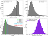 |
Fig. 1 Characterization of the Kepler targets. Top-left: distribution of apparent Gaia G-band magnitudes. The targets are mostly concentrated in the 10 < G < 16 mag range. Top-right: distribution of Gaia distances. The distribution peaks around ~1 kpc. Bottom-left: distribution of RUWE values, with the vertical lines indicating RUWE = 1.0 (green), 1.2 (cyan), and 1.4 (red). From this, RUWE binaries are later identified in Sect. 4. Bottom-right: distribution of calibrated metallicity values, for the subsample with best-quality gspspec data. The distribution peaks around [M/H] = 0 dex, in agreement with the literature. |
3.3 CMD sample
The stars that passed all the quality cuts from Sect. 3.1 can be reliably placed on the CMD, hence, for the remainder of this paper we refer to them as the “CMD sample”. We calculated de-reddened colors as
![Mathematical equation: $\[(B P-R P)_0=\left(B P-A_{B P}\right)-\left(R P-A_{R P}\right),\]$](/articles/aa/full_html/2025/04/aa48735-23/aa48735-23-eq1.png) (1)
(1)
and absolute magnitudes as
![Mathematical equation: $\[M_{G_0}=\left(G-A_G\right)+5-5 \log _{10}(d),\]$](/articles/aa/full_html/2025/04/aa48735-23/aa48735-23-eq2.png) (2)
(2)
where ABP, ARP, and AG are the extinction values in the corresponding bands as obtained in Appendix E, and d is the Gaia distance in pc. Their uncertainties were calculated from error propagation as
![Mathematical equation: $\[\sigma_{(B P-R P)_0}=\sqrt{\sigma_{B P}^2+\sigma_{A_{B P}}^2+\sigma_{R P}^2+\sigma_{A_{R P}}^2}\]$](/articles/aa/full_html/2025/04/aa48735-23/aa48735-23-eq3.png) (3)
(3)
and
![Mathematical equation: $\[\sigma_{M_{G_0}}=\sqrt{\sigma_G^2+\sigma_{A_G}^2+\left(\frac{5}{\ln (10)} \frac{\sigma_d}{d}\right)^2}.\]$](/articles/aa/full_html/2025/04/aa48735-23/aa48735-23-eq4.png) (4)
(4)
The median errors are σ(BP−RP)0 = 0.049 mag and σMG0 = 0.063 mag. The color errors are heavily dominated by the extinction uncertainties (particularly σABP), while for the magnitude errors both distance and extinction uncertainties contribute almost equally (with the former being slightly more prominent). The (BP − RP)0, σ(BP−RP)0, MG0, and σMG0 values are reported in Table A.1.
We show the CMD and Hess diagram of this sample in Figure 2, with the median error bars shown as the purple marker for reference. The stars observed by the Kepler mission span a range of evolutionary stages, with the targets being mostly concentrated towards MS solar-like stars (Huber et al. 2014; Berger et al. 2020; Wolniewicz et al. 2021).
The stars excluded by the quality cuts of Sect. 3.1 are not shown in the CMD. They are identified as such in Table A.1 by having Flag CMD = notinCMDsample, and amount to 8.9% of the Kepler sample (17 467 stars). We note that some of these do have measured magnitudes and distances, and hence could have been plotted on the CMD. We have chosen to restrict the CMD sample to a more high-quality data set, but we nonetheless report all the relevant data in Table A.1 for interested readers.
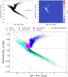 |
Fig. 2 Absolute and de-reddened Gaia CMD of the Kepler targets. Top-left: CMD sample described in Sect. 3. The purple marker illustrates the median error bars. Top-right: Hess diagram of the CMD sample. Bottom: CMD sample, with the stars color-coded according to the CMD categories we define in Sect. 3. The black lines illustrate the borders of the CMD regions. |
3.4 CMD categories
We now classify the Kepler stars into different categories based on their locations on the CMD. The results of this classification are shown in the bottom panel of Figure 2, and reported in Table A.1 by the Flag CMD column.
We begin by broadly defining the CMD regions occupied by some of the main evolutionary stages, namely MS, subgiant branch (SGB), and red giant branch (RGB) (e.g., Donada et al. 2023). For this, we chose to use PARSEC4 (PAdova and tRieste Stellar Evolutionary Code; Bressan et al. 2012; Chen et al. 2014; Nguyen et al. 2022), as this family of models reports the SGB separated from the MS and RGB phases5. We downloaded a suite of PARSEC isochrones, in the range of 6.60 < log10(age/yr) < 10.13 (in steps of 0.01 dex), with [M/H] = 0 dex (see Sect. 3.6 for a discussion on the metallicity-dependence). We display their CMD in the top-left panel of Figure 3, and color-code the points according to their evolutionary stage (MS in cyan, SGB in pink, and RGB in blue). From this, we used Python’s alphashape package to delineate the borders that separate the regions, and applied them on the CMD of the Kepler sample.
We find the PARSEC SGB and RGB regions to be clearly separated in the top-left panel of Figure 3, with no evolved star populating absolute magnitudes MG0 ≳ 4 mag. We used the borders of these regions on the CMD sample and classified the stars that fall to the right of the PARSEC SGB/RGB limit as “Giant Branch”. This region, which includes stars on the RGB, red clump (RC), and asymptotic giant branch (AGB), is not further subdivided as performing a detailed distinction between them is beyond the scope of this paper. These correspond to 11.2% of the Kepler sample (22 098 stars), and we show them as blue points in Figure 2.
The separation between the PARSEC MS and SGB, on the other hand, is not as straightforward. As shown in the top-left panel of Figure 3, some overlap exists in the region of the blue loop of stars (where the cyan and pink points coincide). As stars in this CMD location cannot be cleanly classified as either MS or SGB in a global sense (rather, the specific classification depends on the evolutionary stage of each star), we adopted a conservative approach and defined this overlap region as its own category. We defined this region as “Overlap Dwarf/Subgiant”, corresponding to 2.8% of the sample (5578 stars), and targets that fall inside it are shown as yellow points in Figure 2. Again based on the top-left panel of Figure 3, the stars located in between the Overlap Dwarf/Subgiant and Giant Branch regions were given the “Subgiant” classification. These correspond to 13.2% of the sample (25 901 stars), and are shown by the fuchsia points in Figure 2.
We note that some RC stars appear to scatter to the Subgiant region (fuchsia points with MG0 ≲ 0.84 mag in Figure 2). We examined their gspspec metallicities and found that they correspond to subsolar-metallicity stars for which their bluer colors place them to the left of the solar-metallicity SGB/RGB limit. These nonetheless amount to a small number of targets, as illustrated on the zoomed-in Hess diagram in the top-right panel of Figure 3. We assess the reliability of our CMD classification in Sect. 3.6, where the impact of metallicity is discussed, and targets with extreme [M/H] values are flagged.
We also note the presence of 38 stars (0.02% of the sample) with CMD locations that coincide with the white dwarf sequence (e.g., Gaia Collaboration 2018a). A Simbad6 search returned that all of them had been previously identified as either confirmed or candidate white dwarfs in the literature (Maoz et al. 2015; Doyle et al. 2017; Gentile Fusillo et al. 2021). To avoid confusion with the lower-CMD categories we define below, we delineated the “White Dwarf” region as that with MG0 > 3.9(BP − RP)0 + 9, with the targets inside it appearing as the grey points in Figure 2. We note that our White Dwarf region is similar to that of El-Badry et al. (2021) (see also Gaia Collaboration 2018a and Gentile Fusillo et al. 2021).
Proceeding with the rest of the CMD, except for the aforementioned white dwarfs, the stars that fall underneath the border defined by the regions Overlap Dwarf/Subgiant, Subgiant, and Giant Branch, may all be technically classified as MS stars. Nonetheless, we aimed for a more detailed classification motivated by the presence of two interesting populations. First, a small but noticeable fraction of the targets scatter below the MS. Assuming their CMD locations are correct, these targets likely correspond to a mix of hot subdwarfs, metal-poor MS stars, and cataclysmic variables (CVs), i.e., interacting binaries consisting of an MS star and a white dwarf (e.g., see Abril et al. 2020 and Dubus & Babusiaux 2024 for illustrations of their Gaia CMD). Second, the top panels of Figure 2 show an overdensity of MS stars with (BP − RP)0 ≳ 0.9 mag that are slightly more luminous than the bulk population. These systems likely correspond to unresolved binaries (e.g., Hurley & Tout 1998; Lewis et al. 2022), with their exact CMD location being determined by their mass-ratio, age, and metallicity values. Although finding multiple systems in this way is more straightforward when done for star clusters (given the common age and metallicity of their members; Li et al. 2020; Pang et al. 2023), we attempted a global CMD identification of photometric binaries in the Kepler field (see also Gordon et al. 2021; Messias et al. 2022; Canto Martins et al. 2023).
To rigorously define these two under- and over-luminous CMD populations, we proceeded as follows. We first determined the lower envelope of the MS CMD distribution. This was calculated as a smoothed version of the running 99.5th percentile of MG0 values as a function of (BP − RP)0 color. This lower envelope is illustrated as the red dashed line in the bottom-left panel of Figure 3. We defined the CMD region below the lower envelope as “Uncertain MS” (i.e., towards larger MG0 values). This region corresponds to 0.4% of the full Kepler sample (828 stars), and targets that fall inside it are shown as the red points in Figure 2.
Regarding the photometric binary stars, we first defined the bluest color of our search for these targets as (BP − RP)0 = 0.9 mag, corresponding to Teff ~ 5400 K (e.g., Pecaut & Mamajek 2013). This limit was set to avoid misclassifying the stars that are leaving the MS and populating the turn-off region as photometric binaries (e.g., Simonian et al. 2019, 2020). Then, for each MS star with (BP − RP)0 > 0.9 mag, we calculated the difference between its absolute magnitude and that of the lower envelope evaluated at its (BP − RP)0 color. We name this quantity ΔMG0 and report it in Table A.1. The distribution of ΔMG0 values is shown in the bottom-right panel of Figure 3. We fit the ΔMG0 distribution as the sum of two Gaussians. One of these Gaussians represents the population of photometric binaries (with best-fit parameters μPhot.Bin. = −0.910, σPhot.Bin. = 0.391, and amplitudePhot.Bin. = 497), and the other represents the population of single dwarfs (with best-fit parameters μsingle = −0.496, σSingle = 0.166, and amplitude Single = 1635). We then found the value at which both Gaussians contributed equally, ΔMG0 ≡ Δs ≈ −0.758 mag, and took this as the border between the regions (vertical green line in the bottom-right panel of Figure 3). This corresponds to a truncated version of the lower envelope shifted by Δs (i.e., towards higher luminosities), as shown by the green dashed line in the bottom-left panel of Figure 3. We defined the region of MS stars more luminous than this as “Photometric Binary”, corresponding to 7.2% of the sample (14 117 stars), with targets that fall inside it shown as the green points in Figure 2.
The double-Gaussian fit was performed in the entire (BP − RP)0 > 0.9 color range, and therefore the results are valid in a global sense. We nonetheless remark that the density of stars decreases towards redder colors, and the MS gets wider and more diffuse beyond (BP − RP)0 ≳ 2 (see Figure 2), making the separation between photometric binaries and the MS more uncertain. We also note that the value of Δs ≈−0.758 mag is close to the theoretically expected magnitude shift between an MS star and an unresolved equal-mass photometric binary of the same color, Δm = −2.5 log10(2) = −0.753 mag (Hurley & Tout 1998). For this comparison, we highlight the importance of using an appropriate distance indicator. Had we used the Bailer-Jones et al. (2021) photogeometric distances instead of the parallax inverse, an inaccurate Δs, and therefore Photometric Binary CMD region, would have been obtained. This is because the photogeometric Bailer-Jones et al. (2021) CMD prior did not include a population of photometric binaries (it rather assumed all stars to be single sources), hence causing a systematic shift in their distances (see their Section 5.5).
Finally, the remaining region of MS stars, bounded by the evolved and Photometric Binary regions at higher luminosities (lower MG0 values), and by the Uncertain MS region at lower luminosities (higher MG0 values), was defined as the “Dwarf” region. This corresponds to 56.3% of the Kepler sample (110 735 stars), and is shown as the cyan points in Figure 2.
The sample sizes of all the CMD categories are summarized in Table 1. We display the full extent of the CMD regions, and overlay them on the Hess diagram, in Appendix F. While not perfect, our approach allows a straightforward classification of the Kepler stars based on their CMD locations, which can be further characterized in follow-up studies.
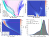 |
Fig. 3 Characterization of the CMD regions presented in Sect. 3. The top-left panel shows the suite of PARSEC models we used to define the upper-CMD regions, and the projections of these onto the Hess diagram are displayed in the top-right panel. The bottom-left panel shows the Hess diagram and borders of the lower-CMD regions. The bottom-right panel shows the distribution of ΔMG0 values we used to define the Photometric Binary region. |
Categories identified in this work.
3.5 Impact of metallicity
The CMD regions of Sect. 3.4 were derived from a suite of PARSEC models at solar-metallicity for the evolved regions, and a sample of mostly solar-metallicity stars for the MS regions (see Figure 1). Although spectroscopic metallicities are not available for most stars in our sample, and performing a star-by-star classification is beyond the scope of this paper, we can assess the impact of global metallicity changes. We tested the robustness of our CMD categories against the effects of metallicity in three steps: assuming a global solar-metallicity (Sect. 3.5.1), assuming a moderate metallicity change given the typical scatter (Sect. 3.5.2), and analyzing the metal-poor and metal-rich tails of the distribution (Sect. 3.5.3).
3.5.1 Monte Carlo sampling assuming solar metallicity
We first examined the confidence of the aforementioned CMD categories ignoring any direct metallicity effects. We quantified this by calculating the probability that a given star recovers its assigned CMD category from Sect. 3.4 (i.e., the Flag CMD column from Table A.1), given the uncertainties on its CMD position. We performed a Monte Carlo simulation and sampled the CMD location of each star Ns = 1000 times following Gaussian distributions ((BP − RP)0, σ(BP − RP)0) for color and (MG0, σMG0) for magnitude. For each sampling, we inferred the CMD category given the regions in the bottom panel of Figure 2. Then, we calculated the number of times that the assigned CMD category was recovered and divided it by Ns. We call this the “probability of CMD category” (PCMD), which ranges from 0 to 1. For instance, a star where the assigned CMD category from Sect. 3.4 was found in 750 of the 1000 samplings has a value of PCMD = 0.75. We report the PCMD values in Table A.1.
We show the distribution of the PCMD values as the filled histogram in the top panel of Figure 4. The distribution is heavily concentrated at values of PCMD≈1 (note the logarithmic y-axis), with a median value of PCMD = 0.90. More specifically, 96% of the CMD sample has PCMD ≥ 0.50, and 77% of it has PCMD ≥ 0.70. In the bottom panel of Figure 4, we show the CMD projection color-coded by the PCMD values (in the same color scheme as the top panel). The diagram illustrates that the targets with low PCMD values correspond to stars located near the boundaries of the CMD regions, i.e., stars more prone to scattering to different CMD regions given their measurement uncertainties. Accordingly, given the smaller area it covers on the CMD, the Overlap Dwarf/Subgiant region has the highest fraction of stars with lower PCMD values. Overall, however, the fact that most of the stars have high PCMD values demonstrates the robustness of our CMD categories for solar-metallicity targets.
3.5.2 Monte Carlo sampling given typical metallicity scatter
We tested the impact of the solar-metallicity assumption by comparing the regions that the evolved populations occupy in suites of metal-poor and metal-rich models. We illustrate these in Appendix G, where we overlaid the borders of the CMD regions defined at [M/H]=0, with PARSEC suites at [M/H]=−0.3 dex and [M/H]=+0.3 dex. The comparison revealed that, at a global level, the regions shift by ![Mathematical equation: $\[\frac{\mathrm{d}(B P{-}R P)_{0}}{\mathrm{~d}[\mathrm{M} / \mathrm{H}]} \sim 0.3\]$](/articles/aa/full_html/2025/04/aa48735-23/aa48735-23-eq5.png) mag/dex and
mag/dex and ![Mathematical equation: $\[\frac{\mathrm{d} M_{G_{0}}}{\mathrm{~d}[\mathrm{M} / \mathrm{H}]} \sim 0.9\]$](/articles/aa/full_html/2025/04/aa48735-23/aa48735-23-eq6.png) mag/dex (i.e., getting redder and less luminous with increasing metallicity).
mag/dex (i.e., getting redder and less luminous with increasing metallicity).
To examine the impact that moderate metallicity shifts had on our CMD classification, we repeated the Monte Carlo sampling from Sect. 3.5.1 and incorporated the effects of the unknown spectroscopic metallicity for most targets. We took these global color- and magnitude-shifts due to metallicity and multiplied them by the standard deviation of the gspspec metallicity distribution (bottom-right panel of Figure 1), σ[M/H],gspspec = 0.2 dex. Thus, at the 1σ level, the global shifts in color and magnitude due to the unknown metallicity were 0.06 and 0.18 mag, respectively. We took these shifts as systematic errors and added them in quadrature with the nominal errors from Sect. 3.3. This increased the median errors to σ(BP−RP)0 = 0.077 mag and σMG0 = 0.191 mag.
We re-ran the simulation from Sect. 3.5.1 with these inflated errors, and show the resulting PCMD distribution as the green line in the top panel of Figure 4. As could be expected due to the larger error bars, the fraction of targets with very high probability decreases (i.e., they are more likely to scatter to other CMD regions). Nevertheless, the median PCMD value is only moderately reduced (0.90 before vs. 0.73 now), and the fraction of the sample with PCMD ≥ 0.50 remains high (96% before vs. 93% now). Thus, we conclude that our overall CMD classification is robust against moderate (1σ, or ≈0.2 dex) metallicity changes. We report these revised probability values in Table A.1 as PCMD,[M/H].
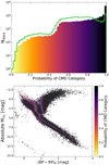 |
Fig. 4 Validation of the CMD categories via the Monte Carlo method presented in Sect. 3.6. Top: Logarithmic distribution of the probability of CMD category parameter, PCMD. The filled histogram represents the fiducial simulation (Sect. 3.5.1), while the open histogram represents the simulation that includes metallicity effects (Sect. 3.5.2). Bottom: CMD projection color-coded by the fiducial PCMD values. Most of the stars have high PCMD values, indicating that their assigned CMD categories are reliable. Targets with low PCMD values are located near the boundaries of the CMD regions (see bottom panel of Figure 2), and their CMD categories are consequently less reliable. |
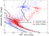 |
Fig. 5 Metallicity impact on the CMD classification. The blue and red points show, respectively, the metal-poor and metal-rich tails (beyond 2σ) of the Andrae et al. (2023b) metallicity distribution. Our CMD classification loses accuracy towards extreme-metallicity values, and this effect is enhanced in certain regions of the CMD. |
3.5.3 Misclassification at the tails of the metallicity distribution
Naturally, our CMD classification loses accuracy towards more extreme (non-solar) metallicity values. Although we lack spectroscopic metallicities for most targets, complementary data sets that leverage the lower resolution Gaia spectrophotometry can provide useful estimates. With this aim, we used the metallicities from Andrae et al. (2023b)7, which are by construction on the APOGEE DR17 scale (Abdurro’uf et al. 2022). Although subject to larger uncertainties compared to higher resolution spectroscopy, the Andrae et al. (2023b) values allowed us to test the effects of metallicities that deviate considerably from solar on the CMD classification.
For this purpose, we selected stars with Andrae et al. (2023b) metallicities beyond the 2σ limits of the distribution for the Kepler targets, namely those with [M/H] values below the 2.3rd and above the 97.7th percentiles (which translate to [M/H] < −0.63 dex and [M/H] > +0.29 dex, respectively). These correspond to 7672 out of the 168 635 targets found by crossmatching our sample with Andrae et al. (2023b). Figure 5 illustrates these metal-poor and metal-rich targets as the blue and red points, respectively. The metallicity effects are readily apparent, with the metal-poor (metal-rich) subset being displaced from the fiducial solar-metallicity CMD regions towards bluer (redder) colors and brighter (fainter) magnitudes, respectively. This demonstrates that our CMD classification is not accurate for such metallicity-extreme targets. These deviations affect some regions of the CMD more heavily, of which we highlight three: metal-poor MS stars shifting to the Uncertain MS region, metal-rich MS stars shifting to the Photometric Binary region, and metal-poor RC stars shifting to the Subgiant region.
We flag these targets via the “Flag Metal-Poor Tail” and “Flag Metal-Rich Tail” columns in Table A.1. As demonstrated in Figure 5, these stars are more prone to having inaccurate CMD classifications, and thus their Flag CMD labels should be used with extreme caution (especially for the three aforementioned cases). Nonetheless, we note that even though their CMD categories might be mistaken, their CMD locations are accurate and reliable.
3.6 Validation
3.6.1 Comparison with asteroseismology
To validate the CMD categories with an external reference, we performed a comparison with the asteroseismic catalogs of evolved stars from Yu et al. (2018) and Yu et al. (2020). Combining both data sets, they report a list of 18 604 unique KIC IDs. 92.1% of these (17 133 stars) pass our CMD quality cuts, and we examined the classification flag we assigned to them. In our catalog, most of their stars are classified as Giant Branch (97.7%), followed by the Subgiant category (2.2%). Combining these, they add up to 99.8% (17 105 stars) of the asteroseismic sample being in evolved CMD categories, in excellent agreement with expectations. The remaining 0.2% of the sample belongs to the other CMD categories, with 24 out of 28 being stars found in the Dwarf region. This likely hints at targets with contamination in their Kepler light curves due to bright neighboring stars (see Sect. 6).
We performed an analogous comparison with APOKASC-3 (Pinsonneault et al. 2025), which combines Kepler asteroseismology with APOGEE spectroscopy (Abdurro’uf et al. 2022) to derive stellar parameters. Importantly for our purposes, they derive evolutionary states, thus providing a comparison point for our CMD classification. The APOKASC-3 catalog reports a list of 15 808 KIC IDs, 88.4% of which (13 977 stars) pass our CMD quality cuts. Restricting the comparison to 13 626 targets classified as “RGB”, “RC”, or “RC/RGB” in APOKASC-3, we classify 96.6% of them (13 167 stars) as CMD Giant Branch and 3.2% of them (441 stars) as CMD Subgiant, with the remaining 0.1% (18 stars) being classified in the other CMD categories. The excellent agreements with these independent catalogs further validate our CMD classification scheme.
3.6.2 Comparison with Gaia DR3 evolutionary stages
As part of the Astrophysical Parameters table, Gaia DR3 reports the analysis of the final luminosity age mass estimator (FLAME) module (Creevey et al. 2023; Fouesneau et al. 2023). In brief, this module takes as input stellar parameters from gspphot and/or gspspec, extinction from gspphot, and distance estimates (parallax inverse or gspphot distance) to produce stellar mass as well as evolutionary parameters by comparing with BASTI solar-metallicity models (Hidalgo et al. 2018). One of the derived properties is the evolstage_flame (ϵ), which quantifies the evolutionary stage of stars. We compared this parameter with our CMD categories.
To facilitate the analysis, we translated the ϵ values to the three labels defined in Section 3.3.2 of Fouesneau et al. (2023), namely 100 ≤ ϵ ≤ 420 as MS, 420 < ϵ ≤ 490 as SGB, and 490 < ϵ as RGB. For the subset of stars in common, we compared these labels with our CMD flags8 from Sect. 3.4. We found agreements of 93.9% for MS stars, 68.0% for SGB stars, and 81.6% for RGB stars.
Regarding their overall comparison, despite differences in the specific modeling (PARSEC vs. BASTI) and input data choices (particularly extinctions and distances), the good global agreement with FLAME validates our CMD classification. In absolute terms, relative to the full Kepler sample (196 762 stars), our CMD classification is available for an extra 8% of targets than the FLAME evolstage_flame parameter (179 295 vs. 163 314, respectively). Moreover, our analysis identifies additional categories of interesting populations that are relevant for complementary studies (e.g., photometric binaries and their role in stellar rotation; Stauffer et al. 2018).
3.7 Caveats
The CMD classification presented throughout Sect. 3 will allow searches of interesting populations for follow-up studies (see Sects. 5–7). Naturally, however, the procedure we adopted carries assumptions and simplifications that must be considered when using it. We now discuss the caveats of the method and potential improvements for future works:
In this paper we only analyzed the Gaia DR3 MG0 vs. (BP − RP)0 CMD. This could be complemented by also leveraging photometry from other surveys (e.g., 2MASS, ALLWISE, Pan-STARRS; Skrutskie et al. 2006; Wright et al. 2010; Chambers et al. 2016). Moreover, the classification was based on photometric and astrometric data, but the use of spectroscopic (log(g), Teff, [M/H) and asteroseismic (Δν, νmax) parameters could help improve the methodology (e.g., Pinsonneault et al. 2014, 2018, 2025; Serenelli et al. 2017).
The photometric analysis was based on the mean Gaia DR3 magnitudes (i.e., phot_g_mean_mag, phot_bp_mean_mag, and phot_rp_mean_mag). Thus, the CMD classification and quality cuts might not be fully accurate or appropriate for stars that exhibit photometric variability. Indeed, some of these targets have time-dependent CMD locations (e.g., see Figure 11 of Gaia Collaboration 2019). We further discuss this in Sect. 7.
We only used the PARSEC models as a reference for the CMD classification. Thus, complementing the analysis with other families of stellar models (e.g., MIST, DSEP; Choi et al. 2016; Dotter et al. 2008) could further refine and validate the categories defined here.
For simplicity, the classification ignored the presence of certain evolutionary stages (e.g., pre-MS) and other types of systems (e.g., symbiotic stars with white dwarf companions, where the surrounding nebula and circumstellar material can influence the measured flux and increase the extinction; Munari 2019). Hence, if present, these stars will be misclassified by the Flag CMD column in Table A.1, as likely more than pure Gaia CMD data is required to reliably identify them (e.g., Merc et al. 2020, 2021). For instance, in the case of pre-MS stars, if present in the sample, they would likely be classified in the Photometric Binary region. We nonetheless note that young stars are not expected in the Kepler field given its Galactic latitude (Zwintz & Steindl 2022).
The Kepler field is a population of mixed stellar ages and metallicities. Therefore, although based on our own (Figure 1) as well as the literature (Ren et al. 2016; Zong et al. 2018) metallicity distribution, our assumption of a global solar metallicity for the fiducial CMD analysis introduced inaccuracies in the classification. These were quantified for metallicity values in the best (solar), typical (1σ scatter), and extreme (beyond 2σ) scenarios in Sect. 3.5. Nevertheless, a future improvement would be to perform the CMD classification on a star-by-star basis with knowledge of the spectroscopic metallicities. At the moment, 12.2% of the Kepler sample have gspspec metallicities (4.3% of them being the most reliable; see Appendix B) from the Gaia DR3 RVS (radial velocity spectrometer; Recio-Blanco et al. 2023). As initially demonstrated in Sect. 3.5.3, however, this fraction may be significantly expanded in future works using novel data sets (e.g., Andrae et al. 2023b; Zhang et al. 2023; Khalatyan et al. 2024) that leverage the lower-resolution XP spectra (De Angeli et al. 2023; Montegriffo et al. 2023).
Regarding the Photometric Binary category, given the aforementioned mix of stellar ages and metallicities present in the sample, our decisions regarding its color and magnitude extent might not fully suit all purposes. To aid in this, in Table A.1 we report the ΔMG0 values, from which readers may design their customized selection cuts.
We used the latest Gaia DR3 parallaxes and photometry, and attempted to ensure well-measured magnitudes, colors, and distances via the quality cuts applied in Sect. 3.1. In the future, thanks to upcoming Gaia data releases, more precise CMD placement will be possible, and a larger sample may be classified thanks to more stars passing the quality cuts.
4 Binary characterization
Binary (and higher-order multiple) systems are of crucial importance in astrophysics (Duquennoy & Mayor 1991; Raghavan et al. 2010; Torres et al. 2010; Duchêne & Kraus 2013; Prša 2018; Serenelli et al. 2021). More specifically, binary stars observed by the Kepler mission are providing fundamental constraints to numerous problems (e.g., Hambleton et al. 2013, 2016, 2018; Beck et al. 2014, 2022; Sandquist et al. 2016; Lurie et al. 2017; Godoy-Rivera & Chanamé 2018; Gehan et al. 2022).
In this section, we investigated our catalog in search of binary candidates using a range of detection methods (e.g., Gaia Collaboration 2023a). We did this by leveraging astrometric and radial velocity (RV) Gaia data (Sects. 4.1 and 4.2), as well as by crossmatching with binary tables published in Gaia DR3 and complementary literature databases (Sect. 4.3 through Sect. 4.10). We generated a flag for each of these binary categories, and also merged them into a combined one for convenience to users (Sect. 4.11). We report the binary flags in Table A.1, and summarize the number of systems in each category in Table 1. For illustration purposes, Figure 6 shows the CMD projection of these populations.
We highlight that, contrary to the Photometric Binary category described in Sect. 3, the binary categories defined in this section are not subject to the CMD quality cuts from Sect. 3.1, and are completely independent of the Flag CMD classifications from Sect. 3.4. Thus, the systems classified as binary candidates in Sect. 4 that lack CMD information, are absent from Figure 6. Analogously, while some overlap exists, the binary categories of this section are defined independently of the Photometric Binary CMD category from Sect. 3.
4.1 RUWE
For a given star, the RUWE value is an astrometric parameter that characterizes how appropriate the Gaia single-star solution is (Gaia Collaboration 2021; Lindegren et al. 2021b). By construction, well-behaved single stars have RUWE values of around 1.0 (Lindegren 2018), with larger values indicating binarity (Belokurov et al. 2020; Penoyre et al. 2020; see also Fitton et al. 2022 for other applications). Since its introduction, it has been widely used in the literature to characterize binary candidates, with typical RUWE thresholds between 1.2 and 1.4 (e.g., Berger et al. 2020; Ziegler et al. 2020; Kervella et al. 2022; Penoyre et al. 2022).
The RUWE distribution for the targets is shown in the bottom-left panel of Figure 1. From this, we classified all the stars with RUWE ≥1.4 as binary candidates (dotted red line), which correspond to 12.2% of the Kepler sample (23 973 stars). The CMD projection of this subset is shown in the top-left panel of Figure 6, which illustrates that it spans the entirety of the CMD. Interestingly, this includes the Photometric Binary region from Sect. 3, thus providing further evidence of its binary nature. The RUWE binaries are identified as such in Table A.1 via the column “Flag RUWE”.
As this selection cut may be too stringent for certain purposes, and some users may wish to define their customized selections (e.g., Castro-Ginard et al. 2024), we also report the RUWE values in Table A.1 for completeness. For instance, had we adopted a less stringent threshold of RUWE ≥1.2 (dashed cyan line in Figure 1), we would have classified 15.7% of the Kepler sample (30 798 stars) as binary candidates.
Additionally, we note that the RUWE parameter does carry limitations for binary identification. Recently, Beck et al. (2024) showed that binary systems detected through other techniques may often still appear as having RUWE values below the binary threshold (e.g., for the literature catalog of spectroscopic binaries discussed in Sect. 4.7, they found that ~40% of systems have RUWE ≤1.4). Beck et al. (2024) concluded that targets with high RUWE values are typically systems located close to Earth with longer orbital periods (see their Figure 4). Thus, these systems can more easily produce a clear astrometric signature of binary motion in Gaia. This highlights the importance of using complementary binary detection methods, as we do in the following subsections.
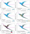 |
Fig. 6 Characterization of the binary categories defined in Sect. 4. The panels display the CMD projection of the RUWE, RV Variable, NSS, Kepler + Gaia EB, SB9 + NEA + HGCA, and WDS binary samples, respectively. In all the CMDs, we show the separation between MS and evolved stars as guidance (dashed fuchsia line). The number of systems in each category is summarized in the bottom-right corner. The CMD projections help to illustrate the selection effects of each category (see Sect. 4 for details). |
4.2 RV variable stars
RV variations are a useful means of identifying binary systems. In Gaia DR3, mean RV values are available for 51.7% of the Kepler sample (101 756 stars). Although the full epoch Gaia RV measurements will not be made available until DR4 (Gaia Collaboration 2023d; but see also Gaia Collaboration 2023c), the DR3 does contain RV variability indices. We used the prescription reported by Katz et al. (2023) to identify targets that can be classified as RV variables based on their RV scatter. In brief, the selection examines the consistency and noise of the RV time series9. While the Katz et al. (2023) criteria can be used for both binary systems and variable stars (e.g., Cepheids and RR Lyraes; see their Section 11), we find the overlap between both categories to be limited10 for our target sample. Thus, we attributed the RV variability signal as coming predominantly from the presence of unresolved companions, and classified these systems as binary candidates (e.g., Cao & Pinsonneault 2022; Patton et al. 2024; Silva-Beyer et al. 2023).
By following this approach, we classified 4072 targets as RV variables (2.1% of the Kepler sample). The CMD projection of this subset is shown in the top-right panel of Figure 6, which illustrates that this criterion is biased towards more luminous targets, scarcely populating the region of MG0 ≳ 6 mag. These RV variable binary candidates are identified as such in Table A.1 via the column “Flag RV Variable”.
4.3 Gaia DR3 non-single stars
Gaia DR3 published over 800 000 solutions for candidate nonsingle stars (NSS) systems (Gaia Collaboration 2023d,a). This sample is comprised of binaries flagged under different solution types and includes astrometric, spectroscopic, and eclipsing binaries (Halbwachs et al. 2023; Holl et al. 2023; Gosset et al. 2025).
We examined the non_single_star column in the gaiadr3.gaia_source table and found 4005 Kepler targets (2.0% of the sample) flagged as NSS. The CMD projection of this subset is shown in the middle-left panel of Figure 6, which illustrates that it virtually spans the entirety of the CMD (see also Figure 4 of Gaia Collaboration 2023a). These NSS binaries are identified as such in Table A.1 via the column “Flag NSS”. We investigate them in more detail in Appendix H, where the “NSS Type” and “NSS Tables” columns of Table A.1 are generated.
4.4 Kepler eclipsing binary stars
Numerous searches for eclipsing binary (EB) signatures have been performed in the Kepler light curves (e.g., Coughlin et al. 2011; Prša et al. 2011). In particular, the Villanova catalog11 of Kepler EBs provides a detailed inventory and characterization of such systems. For completeness, we downloaded the most recent version12 of the catalog reported by Kirk et al. (2016) and crossmatched it with our sample. We found 2865 targets in the Kepler EB catalog (1.5% of our target list). The CMD projection of this subset is shown in cyan in the middle-right panel of Figure 6, and is in good qualitative agreement with other literature studies (e.g., Mowlavi et al. 2023). These Kepler EBs are identified as such in Table A.1 via the column “Flag EB Kepler”.
4.5 Gaia eclipsing binary stars
We complemented the above with the Gaia DR3 catalog of EB candidates (Mowlavi et al. 2023). These systems were identified from photometric variability criteria applied on their G-band light curves, and a fraction of them also have NSS orbital solutions (see also Sect. 4.3). We crossmatched with the gaiadr3.vari_eclipsing_binary table and found 854 targets (0.4% of the sample). The CMD projection of this subset is shown in orange in the middle-right panel of Figure 6. These Gaia EBs are identified as such in Table A.1 via the column “Flag EB Gaia.”
In our catalog, both Kepler and Gaia EB flags are reported independently. We note, however, that a large overlap exists between them, in the sense that most of the Gaia EBs are contained within the Kepler EB sample. More specifically, 801 out of 854 Gaia EBs (94%) are also flagged as Kepler EBs. Comparing the orbital periods in this overlap sample, we find 661 out of 801 systems (83%) to have values along the 1:1 relation (fractional differences <0.1%). This is in good agreement with the literature comparisons from Mowlavi et al. (2023).
4.6 Other Gaia variable binaries
Beyond the aforementioned EBs (Sect. 4.5), there are other categories of binary candidates that can be flagged based on their Gaia DR3 variability (Rimoldini et al. 2023). We elaborate on the Gaia variability classification for the Kepler targets in Sect. 7. For the purpose of identifying binaries, however, we highlight the following four categories: cataclysmic variables (CV), ellipsoidal variables (ELL), RS Canum Venaticorum variables (RS), and symbiotic variables (SYST). We specifically looked for stars classified in these categories, and found 15 as CV, 0 as ELL, 759 as RS, and 1 as SYST. Their CMD projection is shown later in Sect. 7. For simplicity we grouped them into one category named Gaia variable binaries, amounting to 775 targets (0.4% of the sample). These systems are identified in Table A.1 via the column “Flag Gaia Variable Binary”.
4.7 The 9th catalog of spectroscopic binary orbits
We complemented the characterization by searching for spectroscopic binaries reported in the literature. For this, we used the 9th catalog of spectroscopic binary orbits (SB913) by Pourbaix et al. (2004), which compiles up-to-date information for such targets and currently lists over 4000 systems. In particular, we crossmatched with the latest SB9 version14, following the curation procedure from Beck et al. (2024), which accounted for multiple entries in the catalog and filtered them accordingly (see their Appendix A.1). We found 49 targets in the SB9 catalog (0.02% of the Kepler sample), with no triple systems being found. The CMD projection of this subset is shown as the green diamonds in the bottom-left panel of Figure 6, and illustrates a clear preference for early-type and more luminous stars. These spectroscopic binaries are identified as such in Table A.1 via the column “Flag SB9”.
4.8 NASA exoplanet archive
As many of the Kepler stars have been studied in the context of exoplanet searches, for completeness we also queried the NASA exoplanet archive (NEA)15. Besides its function as an exoplanet database, NEA compiles relevant information for host star characterizations, including from ground-based spectroscopic follow-up. In particular, it includes a flag for binary or higher order systems in the “sy_snum” value, i.e., the number of stars in the system. We found 1979 of the Kepler stars in the NEA table16 of confirmed planets and their hosts. Of these, 71 targets (0.04% of the Kepler sample) have values of sy_snum > 1 and are thus classified as multiple systems. More specifically, 66 targets have sy_snum=2, 4 targets have sy_snum=3 (KIC 4278221, KIC 6278762, KIC 9941662, and KIC 12069449), and 1 target has sy_snum=4 (KIC 4862625). The CMD projection of this subset is shown as the purple squares in the bottom-left panel of Figure 6, with almost all of the targets being located along the MS. These NEA multiple systems are identified as such in Table A.1 via the column “Flag NEA sy_snum”. For completeness, we also include the sy_snum values when available, which can be used to identify the confirmed exoplanet hosts (i.e., those targets with reported sy_snum values).
While not explicitly included in Table A.1, we also checked for the presence of circumbinary planet hosts in the target sample (e.g., see Martin 2018). We found 12 such systems, all classified as NEA binaries. These are: KIC 4862625, KIC 5095269, KIC 5473556, KIC 6504534, KIC 6762829, KIC 8572936, KIC 9472174, KIC 9632895, KIC 9837578, KIC 10020423, KIC 12351927, and KIC 12644769.
4.9 HIPPARCOS-Gaia catalog of accelerations
The Gaia astrometry can be combined with complementary databases, such as the HIPPARCOS mission (ESA 1997). The comparison of precise proper motion measurements at different epochs allows the identification of accelerating stars due to wide companions (e.g., Brandt 2018; Kervella et al. 2022). Brandt (2021) published the HIPPARCOS-Gaia catalog of accelerations (HGCA), which presents a cross-calibration of the HIPPARCOS and Gaia EDR3 astrometry, and accounts for the different frames of reference. The HGCA quantifies the difference between the Gaia EDR3 and long-term proper motions using the χ2 parameter, where values of χ2 ≳ 11.8 correspond to targets with inconsistent constant proper motions at the 3σ level. The HGCA probes the bright limit of our sample, which has a median apparent G ≈ 14.6 mag, as the HIPPARCOS catalog includes targets down to apparent V ≲ 12 mag. In terms of orbital timescales, Escorza & De Rosa (2023) used the HGCA on a sample of RV-confirmed binaries, and concluded that the χ2 ≳ 11.8 threshold is reliable in identifying binaries with periods ≳ 103 days.
We crossmatched our sample with the Gaia EDR3 HGCA, and found 275 entries in common. Of these, 97 targets (0.05% of the sample) have values of χ2 > 11.8. We flag these as binary candidates, and show their CMD projection as the red hexagons in the bottom-left panel of Figure 6. The targets are heavily concentrated on the most luminous parts of the CMD, particularly the giant branch and the upper MS. These HGCA binary candidates are identified as such in Table A.1 via the column “Flag HGCA High χ2.”
4.10 Washington double star catalog
We supplemented the binary search by crossmatching with the Washington double star (WDS) catalog (Mason et al. 2001). This catalog is a benchmark reference for multiple star systems, and currently lists over 150 000 binaries. We crossmatched with the latest WDS version17, and found 2829 Kepler targets (1.4% of the sample). The CMD projection of this subset is shown in cyan in the bottom-right panel of Figure 6, which illustrates that it spans the entirety of the CMD. These WDS binaries are identified as such in Table A.1 via the column “Flag WDS.”
We note that the WDS binaries can be somewhat different from those of earlier sections, as in this case the components may have been resolved in the literature (i.e., visual binaries). This is the case for most of our crossmatch, which allowed us to estimate some properties for them. The median angular separation of our WDS binaries is ≈3.2″, and using their Gaia distances we estimated a median (projected) physical separation of ≈2900 AU. Their distribution of magnitude difference (in the sense of primary minus secondary) has 16th, 50th, and 84th percentiles of ≈−0.9, −3.4, and −5.5 mag. To facilitate further analysis of these systems, in Table A.1 we also report the corresponding WDS names when appropriate.
4.11 Union of binary categories
As some readers may want to identify all of the potential binary candidates in our catalog, regardless of their specific flag or detection method, Table A.1 also includes the “Flag Binary Union” column. This flag is the union of all the binary flags introduced in the previous subsections. This subset amounts to 31 334 targets (15.9% of the sample), and it is heavily dominated by the RUWE binary candidates (see Table 1). Note that, as introduced at the beginning of Sect. 4, this category is independent of the Flag CMD classification (and thus does not account for the Photometric Binary category from Sect. 3).
To compare the different binary categories among each other, Figure 7 shows the distributions of their apparent magnitudes, as well as a Venn diagram18. For practical reasons, we only included the four most numerous categories, namely RUWE (purple), RV Variable (green), NSS (red), and Kepler EB (cyan). The magnitude distribution illustrates that the selection of the RV Variable binaries was limited to apparent G ≲ 13.5 mag (inherited from the Gaia DR3 RV availability), while the RUWE binaries span the entire magnitude range. The vertical dotted lines indicate the median of each distribution and correspond to 11.9 mag for the RV Variable, 12.7 mag for the NSS, 14.0 mag for the Kepler EB, and 14.2 mag for the RUWE binary candidates. For reference, the median value of the full Kepler sample is 14.6 mag (see Figure 1).
Regarding the Venn diagram, for instance by comparing the NSS and RV Variable binaries, we found that they share ~40% of their samples (1675 out of the 4072 RV Variable and 4005 NSS targets). More generally, an important finding of this comparison is that a significant fraction of the targets flagged by a given category are often not flagged by the rest. For instance, 81% of the RUWE binary candidates were not found in other categories. Although the WDS binaries are not explicitly shown in Figure 7 to avoid an excessively complicated diagram, these constitute the fifth most numerous category and 65% of them were not found in the other binary samples. Interestingly, considering the criteria shown in Figure 7, 34 targets were classified as binaries by all four categories simultaneously. These findings highlight the power of integrating different binary criteria into one unique catalog.
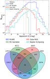 |
Fig. 7 Comparison of the four most numerous binary categories. Top: distribution of apparent G-band magnitudes. The RV Variable and RUWE binary candidates are concentrated at the bright and faint limits of the Kepler sample, respectively. Bottom: Venn diagram. While some categories show a moderate degree of overlap (e.g., RV Variable and NSS), others do not (e.g., RUWE). |
5 Astrometric differences between Gaia data releases and CMD implications
The Gaia mission has provided unprecedented astrometry for over a billion stars, becoming of paramount importance in stellar selections. Given its massive use across the literature, assessing the changes stars may have experienced from one data release to the next is highly relevant, as they could translate into differences in the derived stellar parameters. Global changes of the DR3 relative to the DR2, in terms of astrometric completeness and validation, have already been reported by Fabricius et al. (2021). In this section, we focus on the main star-by-star astrometric differences for the DR3 versus DR2 (Lindegren et al. 2018, 2021b). Specifically for the Kepler targets, we studied how these translate into changes to the CMD locations and classifications. For simplicity, we ignored magnitude and extinction effects, as the photometric systems between DR3 and DR2 are similar, albeit not identical (Riello et al. 2021; Maíz Apellániz & Weiler 2024).
For every Kepler star, we looked for potential DR2 crossmatches using the gaiadr3.dr2_neighbourhood table in the Gaia archive, finding that most DR3 targets have one DR2 counterpart, but a fraction have multiple. The distributions of angular separations and magnitude differences between DR3 and DR2 are heavily concentrated towards Δθ < 0.1″ and |ΔG| < 0.05 mag. We adopted these limits as the tolerances for a reliable crossmatch, prioritizing the nearest target (in terms of Δθ) in case of multiple counterparts.
From these Gaia DR2 IDs, we queried the tables gaiadr2.gaia_source for parallax and gaiadr2_geometric_distance for distance information (Bailer-Jones et al. 2018). To ensure reliable astrometry, we limited the comparison to the stars in the CMD sample (Sect. 3.1), and also imposed a DR2 parallax SNR of ϖ/σϖ > 10, corresponding to a subset of 173 612 stars (88.2% of the Kepler sample). We illustrate the distance comparison between both data releases in the top panel of Figure 8. The density map is heavily centered around the 1:1 line, albeit some scatter extends out to near the 1.5:1 and 1:1.5 ratios. While not explicitly shown, the analogous parallax comparison is equivalent (e.g., with ≈93% and 98% of the subset having parallaxes that agree at the 2σ − and 3σ-levels between DR3 and DR2, respectively).
We now examine the effects of the improved astrometry by comparing the changes in CMD positions due to the updated distance estimates. For this, we computed the difference in the distance modulus values from both data releases (in the sense of DR3 minus DR2),
![Mathematical equation: $\[\Delta \mathrm{DM}=\left(5 ~\log _{10}\left(d_{\mathrm{DR} 3}\right)-5\right)-\left(5 ~\log _{10}\left(d_{\mathrm{DR} 2}\right)-5\right),\]$](/articles/aa/full_html/2025/04/aa48735-23/aa48735-23-eq7.png) (5)
(5)
where dDR3 and dDR2 are the distances from DR3 and DR2 in pc. This new parameter allowed us to easily re-compute absolute magnitudes using the DR2 distances, as MG0,DR2 = MG0,DR3 + ΔDM. We report the ΔDM values in Table A.1, and show its distribution in the middle panel of Figure 8. The excellent overall distance agreement translates to a ΔDM distribution heavily centered at zero (vertical fuchsia line), with tails extending towards both positive and negative values.
At this point, we defined two subsets of outliers from the ΔDM distribution. We selected the stars that lie beyond the 1.5:1 and 1:1.5 distance relations (dashed lines in the top panel of Figure 8), i.e., those with values of ΔDM > 5 log10(1.5/1) = 0.88 mag and ΔDM < 5 log10(1/1.5) = −0.88 mag. These data sets contain 17 and 19 stars respectively, and we show them as the blue and red points in all panels of Figure 8. In the bottom panel of Figure 8, we show the DR3 CMD of the Kepler targets in the grey background, with the ΔDM outliers highlighted in colors. For these outliers, we show two sets of CMD positions, corresponding to the MG0,DR3 (green squares) and MG0,DR2 (yellow crosses) absolute magnitudes, and connect them with the corresponding blue or red lines.
For stars with large ΔDM values (either positive or negative), the CMD illustrates the importance of using the updated DR3 astrometry when deriving stellar properties. For instance, the blue outliers had under-luminous absolute magnitudes in DR2, and many of them went from lying underneath the MS and RC to being right on top of them with DR3. The analogous change in the opposite direction is true for the red outliers, with them going from over-luminous absolute magnitudes to (mostly) landing on higher-density regions. Upon further inspection of these 36 (= 17 + 19) ΔDM outliers, we note that all except four are flagged as RUWE binaries in DR3, thus potentially explaining their astrometric discrepancies.
To generalize the analysis beyond these outliers, we replicated the CMD classification of Sect. 3.4 to the 173 612 stars with ΔDM values. For each star, we inferred the CMD category using its MG0,DR2 absolute magnitude, and compared it with the original CMD classification obtained in Sect. 3 using its MG0,DR3 value. We found that 6348 stars change CMD category between Gaia DR3 and DR2, and these are identified as such by the “Flag Δ DM” column in Table A.1. As may be expected, this sample is dominated by stars with low PCMD values, i.e., stars with unreliable CMD classifications (due to being close to the borders of the CMD regions; see Sect. 3.5.1). Restricting this to targets with higher probabilities, we found 971 stars with PCMD ≥ 0.70, and 171 stars with PCMD ≥ 0.90, that change CMD categories between Gaia DR2 and DR3.
Naturally, these changes hold important consequences for the properties of these stars, and that of their potential planets. For instance, among the stars with changing CMD categories, we found 52 exoplanet hosts according to NEA19. Thus, readers are encouraged to check for potential CMD changes in their target samples using the ΔDM and Flag ΔDM columns in Table A.1. All of the above highlights the importance of our catalog regarding astrometric differences between Gaia DR3 and DR2.
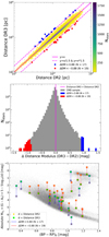 |
Fig. 8 Astrometric comparison between Gaia DR3 and DR2 from Sect. 5. Top: 2D histogram of the distance comparison. Most targets closely follow the 1:1 relation. Middle: Distribution of the distance modulus difference (in the sense of DR3 minus DR2). Stars are heavily centered around ΔDM = 0, but outliers outside the 1.5:1 and 1:1.5 relations are selected for further inspection (blue and red samples). Bottom: CMD projection of the ΔDM outliers, with their DR3 and DR2 positions shown in the green squares and yellow crosses, respectively. The astrometric differences can drive important CMD changes, thus modifying the derived stellar properties. |
6 Complementing Kepler seismic results with Gaia
Mathur et al. (2016) identified over 800 targets with parameters consistent with dwarf stars according to the Kepler Star Properties Catalog (Huber et al. 2014; see also Brown et al. 2011), but where asteroseismic investigations of their light curves revealed oscillations corresponding to giants. They combined these asteroseismic analyses with broadband photometry and derived distances for the targets, finding most of them at several kpc. Furthermore, they reported a series of flags that identify targets with potential contamination in their light curves, namely pollution, blending, crowding, and poor SNRs. In this subsection, we revisit these targets in light of the Gaia DR3 data.
Starting with the 824 stars from Mathur et al. (2016), we found that 27 are either missing from our catalog or lack Gaia distances, and are thus excluded from the following analysis. For the remaining 797 stars, we show the distance comparison between both catalogs in the top panel of Figure 9. Of these, 369 fail the CMD quality cuts from Sect. 3.1, and we show them as black points. These stars are predominantly found ≳5 kpc away and are thus too distant to have well-measured parallaxes.
We now focus on the subset of 428 stars that pass the CMD quality cuts. We split the sample between those that fall inside or outside the 2:1 and 1:2 lines in the distance comparison, hereafter referred to as the targets inside or outside the distance range, respectively. These are shown as the orange and green points in Figure 9, with their sample sizes being 334 and 94 stars. We note that, for the targets outside the distance range, the Mathur et al. (2016) distances are always larger than the Gaia distances.
In the middle panel of Figure 9, we show the Gaia CMD projection of these targets. They occupy noticeably distinct CMD regions, with the subsets inside and outside the distance range appearing predominantly as giants and MS stars, respectively. We interpret this as follows. Those inside the distance range (orange) correspond to targets where the Kepler light curve is dominated by a giant star that matches the Gaia DR3 ID in our catalog (i.e., both Kepler light curve and Gaia DR3 ID recognize the same star, albeit the KIC ID in Huber et al. (2014) is that of a photometric dwarf). On the other hand, those outside the distance range (green) correspond to targets where the Gaia DR3 ID in our catalog is that of a dwarf, but where the Kepler light curve is likely contaminated by a nearby giant star, thus showing asteroseismic oscillations in Mathur et al. (2016) (i.e., both the KIC ID in Huber et al. (2014) and the Gaia DR3 ID recognize the same dwarf star, but the Kepler light curve is dominated by a bright giant in the neighborhood).
We further inspected these targets by including the light curve contamination flags from Mathur et al. (2016). We show these as the smaller inset blue circles in the CMD of Figure 9. Of the 74 flagged stars, 69 of them (93.2%) corresponded to targets outside the distance range, while 5 of them (6.8%) corresponded to targets inside the distance range. Consequently, there is a clear trend for most of the targets with contaminated light curves to coincide with those with large distance discrepancies, providing further evidence for our interpretation. For completeness, we also examined the fraction of targets classified as binaries, and found them to be comparable across both samples (≈7%). Thus, binarity, in terms of the unresolved and resolved categories presented in Sect. 4, does not seem to be a significant factor in the above.
As a final piece of the analysis, we investigated the neighborhoods of these targets by querying the gaiadr3.gaia_source table for other stars in their vicinity. We limited the search to neighbors within Δθ ≤ 20″ and |ΔG| ≤ 6.5 mag. The ΔG vs. Δθ projection of this search is shown in the bottom panel of Figure 9, with the marginalized distribution of each axis on the subpanels, and the number of neighbors (integrating over each subset) displayed in the top-right corner legend. For reference, we indicate the 3.98″ size of the Kepler pixels and its multiples (up to ×5) as the vertical dashed lines. The results illustrate that the targets outside the distance range (green) have preferentially more bright (ΔG ≈ −0.5 to +3 mag), close (Δθ ≈ 3″ to 8″) neighbors than the targets inside the distance range (orange). These overdensities are indeed located within the size of a few Kepler pixels, thus explaining the aforementioned contamination in the light curves.
While other tools are better suited for the analysis of flux contamination in light curves (Schonhut-Stasik & Stassun 2023), our work illustrates the mismatches that such an effect can have on the CMD location of stars. All in all, the above highlights the power of the Gaia data in the study and interpretation of asteroseismic targets.
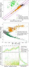 |
Fig. 9 Gaia DR3 analysis of the misclassified stars identified by Mathur et al. (2016) from Sect. 6. Top: distance comparison. The sample was split between targets inside (orange) and outside (green) the 2:1 and 1:2 lines. Middle: Gaia CMD projection. The targets with large distance discrepancies (green) appear predominantly as MS stars in Gaia, and most of them have crowding or blending flags (overplotted blue) in Mathur et al. (2016). Bottom: ΔG vs. Δθ diagram (and marginalized distributions) of the stars’ neighborhoods. The targets outside the distance range have more bright nearby neighbors than the targets inside the distance range, and thus the former are more prone to having contaminated Kepler light curves than the latter. |
7 Gaia variability classification for the Kepler stars
In this section, we extend the analysis of the Kepler stars by leveraging complementary Gaia data products. In particular, we examine the photometric variability information of our targets as reported in Gaia DR3 (Eyer et al. 2023). Such variability analyses are allowed by the multiple-epoch observations of the mission, which span 34 months as of DR3 (e.g., Clementini et al. 2023; Distefano et al. 2023; Lebzelter et al. 2023; Marton et al. 2023; Mowlavi et al. 2023; Ripepi et al. 2023).
We began by studying the phot_variable_flag in the gaiadr3.gaia_source table. This parameter identifies targets with variability in the photometric data (for the subset of sources that Gaia had processed by the release of DR3). We found 13 803 (7.0%) of the Kepler targets classified as VARIABLE, and 182 959 (93.0%) classified as NOT AVAILABLE. We further investigated the subset of VARIABLE targets by querying their variability classification as reported by the best_class_name in the gaiadr3.vari_classifier_result table (Rimoldini et al. 2023). This parameter identifies the best classification for variable sources obtained via statistical and machine learning methods trained on benchmark targets (Gavras et al. 2023). Of the 13 803 VARIABLE stars, we found 13 661 with variability classifications. We report both of these Gaia DR3 parameters in the “Flag Photometric Variability” and “Photometric Variability Class” columns in Table A.1.
We found 19 different classes of variable sources in the sample. Their acronyms, taken verbatim from Gaia DR3, are as follows: SOLAR_LIKE (solar-like star), DSCT|GDOR|SXPHE (δ Scuti, γ Doradus, or SX Phoenicis star), ECL (eclipsing binary), RS (RS Canum Venaticorum variable), LPV (long-period variable), S (short-timescale object), RR (RR Lyrae star), ACV|CP|MCP|ROAM|ROAP|SXARI (α2 Canum Venaticorum, or (magnetic) chemically peculiar, or rapidly oscillating Am- and Ap-type, or SX Arietis star), AGN (active galactic nucleus), SPB (slowly pulsating B-type variable), CV (cataclysmic variable), EP (star with exoplanet transits), SDB (subdwarf B), BE|GCAS|SDOR|WR (B-type emission line, γ Cassiopeiae, S Doradus, or Wolf-Rayet), CEP (Cepheid), YSO (young stellar object), WD (variable white dwarf), SYST (symbiotic variable star), and BCEP (β Cephei). Readers are referred to Rimoldini et al. (2023) for more detailed definitions.
These 19 variability classes are also listed as the labels20 of the bar chart in the top panel of Figure 10. The categories are sorted in decreasing order from the top, based on the number of stars recovered in each, as indicated by the text inside each bar (followed by the number of those that pass the CMD quality cuts in parenthesis). The CMD projection of the sources flagged as variables (e.g., see Gaia Collaboration 2019) is shown in the middle panel of Figure 10. The color-coding is identical to that of their variability class in the top panel, and the marker sizes are larger for smaller samples. Note that, for several categories (e.g., S, CV), only a small fraction (or even none) of the targets are shown on the CMD. Since our CMD analysis of Sect. 3 was based on the mean Gaia DR3 magnitudes (see Sect. 3.7), photometrically variable stars are naturally more prone to failing the CMD quality cuts. Additionally, the CMD placement can only be done for targets that pass the parallax quality cut (see Sect. 3.1), which as expected prevents extragalactic sources from appearing on the CMD (e.g., AGN).
The predominant variability class is SOLAR_LIKE (8441 targets), followed by DSCT|GDOR|SXPHE (2851 targets). Moreover, the CMD of Figure 10 shows that most of the variable targets are located along the MS. A fraction of them extend to evolved regions, such as the LPV, BE|GCAS|SDOR|WR, and CEP classes. Additionally, many stars that may have appeared as CMD outliers, can now be explained by their photometric variability classification. Although only including a few targets, the SDB, YSO, and CV categories occupy CMD regions that are expected given their variability class. We also note that the targets classified as ECL, CV, RS, and SYST are the same binary candidates previously discussed in Sects. 4.5 and 4.6. Other interesting targets are those classified as EP and AGN, which are discussed in more detail in Appendix I.
We now turn to the 142 (= 13 803–13 661) targets flagged as VARIABLE in Gaia DR3 that lack variability classifications in gaiadr3.vari_classifier_result (and are thus absent from the top and middle panels of Figure 10). For completeness, we queried the gaiadr3.vari_summary table, and found that all of them are also in the gaiadr3.vari_short_timescale table, which in turn reports variable candidates that show short-timescale phenomena (<0.5 to 1 day; see also Roelens et al. 2017, 2018). These 142 targets do not appear in any of the other Gaia variability tables, and we thus refer to them as “Gaia short-timescale variable only.” We show their CMD positions as the black squares in the bottom panel of Figure 10. We inspected their CMD categories, and found 80 targets classified as Dwarf, 21 as Subgiant, 14 as Photometric Binary, 8 as Overlap Dwarf/Subgiant, 6 as Giant Branch, 4 as Uncertain MS, and 9 that failed the CMD quality cuts. In terms of their median distance and apparent G-band magnitudes, these targets are more distant (Δd ≈ 500 pc) and slightly brighter (ΔG ≈ 0.5 mag) than their counterparts with gaiadr3.vari_classifier_result classifications. Interestingly, 61 of the 142 targets are flagged as eclipsing binaries from the Kepler light curves (Sect. 4.4). We show these as the overplotted cyan crosses in the bottom panel of Figure 10.
Additional explorations of the over 13 000 photometrically variable targets are left as future work. We encourage the community to further investigate these variable sources by taking advantage of the different observing baselines of the Kepler and Gaia missions (e.g., Hey & Aerts 2024; Zhou 2024).
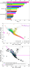 |
Fig. 10 Photometric variability analysis of the Kepler targets from Sect. 7. Top: bar chart of the 19 classes of variable sources found in Gaia DR3. The text inside the bars lists the number of targets in each class (with the size of the CMD subset shown in parenthesis). Middle: CMD projection of the variable sources with classifications. Targets are color-coded following the bars in the top panel, and the symbol size increases for smaller samples. The full CMD sample (grey) is shown for reference in the background. The interpretations of the CMD locations are greatly benefited by the variability classifications in Gaia DR3. Bottom: CMD projection of the “Gaia short-timescale variable only” targets (black squares). A significant fraction of them were found to be Kepler eclipsing binaries (cyan crosses). |
8 Conclusions
The stars observed by the Kepler mission remain a highly relevant sample for studies of stellar, exoplanetary, and Galactic astrophysics. In this paper, we characterized the ~200 000 stars observed by Kepler in light of the recent Gaia DR3. These data provide unprecedented constraints regarding astrometry, photometry, spectroscopy, and stellar parameters.
We used the Gaia DR3 distances and magnitudes, in combination with a series of quality cuts that ensure reliable parameters, and placed the Kepler stars on the absolute and de-reddened CMD (Figure 2). Regarding extinction, we considered a number of maps from the literature. We chose the map that maximizes homogeneity for our sample, and used the comparisons among the different maps to estimate extinction uncertainties. The photometry was de-reddened using the latest Gaia DR3 coefficients, and the photometric, astrometric, and extinction uncertainties were propagated to the reported CMD positions (Table 1). From this, by comparing with stellar models and empirical analyses, we separated the sample into several categories based on CMD location. These include stars classified as: Dwarf, Photometric Binary, Subgiant, Giant Branch, as well as other categories that represent more rare CMD regions (Overlap Dwarf/Subgiant and Uncertain MS). We validated these categories by performing internal tests that considered the associated CMD uncertainties and the effects of metallicity, as well as external tests with asteroseismic catalogs and results from the Gaia DR3 FLAME module. The caveats involved in the classification are discussed.
We also reported several categories of candidate binary systems (Figure 6). These were identified through a number of detection methods applied to the Gaia data, as well as by crossmatching with published Gaia DR3 binary tables and complementary literature data sets. The binary categories are RUWE, RV Variables, Gaia NSS, Kepler eclipsing, Gaia eclipsing, Gaia variables, spectroscopic from the SB9 catalog, multiples from the NASA Exoplanet Archive, HIPPARCOS-Gaia catalog of accelerations, and binaries from the Washington Double Star catalog. We report their respective sample sizes (Table 1) and discuss the different degrees of overlap among them. For convenience to readers, we also report the Binary Union category, which identifies all the targets flagged by any of the binary detection methods.
Additionally, we leveraged the Gaia data to carry out three further characterizations of the Kepler targets. First, we assessed how the astrometric differences between Gaia DR3 and DR2 are translated into changes on CMD location (Figure 8). Second, we revisited a sample of misclassified asteroseismic targets. We found that disagreements in distance estimates between Gaia versus photometric plus asteroseismic constraints are typically caused by mismatches due to bright, nearby neighbors that contaminate the Kepler light curves (Figure 9). Third, we examined the photometric variability flags and classes reported in Gaia DR3. The Kepler targets span 19 different variability categories, and their classifications provide valuable complements to the CMD analysis (Figure 10). Moreover, we found that ~40% of the “Gaia short-timescale variable only” targets correspond to eclipsing binaries as seen by Kepler.
The applications of this catalog are multiple. Our work will aid in the investigation of stellar properties and how they are influenced by stellar architectures and evolutionary stages. For instance, the catalog allows the straightforward selection of single stars or binary candidates, or of stars on the MS or in post-MS phases. Examples include the criteria to exclude binaries (Flag Binary Union = FALSE), focus on MS stars (Flag CMD = Dwarf), select evolved stars (Flag CMD = Subgiant and/or Giant Branch), or target specific binary categories (e.g., Flag RV Variable = TRUE). The same benefits extend to the selection of exoplanet hosts (e.g., McQuillan et al. 2013; Berger et al. 2023), with a preliminary version of the catalog being used by García et al. (2023) to identify single MS planet hosts. The parameters we report allow for valuable characterizations and comparisons, though it is important to consider the assumptions and caveats involved. We make our catalog publicly available (Table A.1) and encourage the community to take full advantage of it as a useful resource in the continued exploration of the stars observed by the Kepler mission.
Data availability
Full Tables A.1 and F.1 are available in electronic form on Zenodo (https://zenodo.org/records/14774100) and full Table A.1 is available at the CDS via anonymous ftp to cdsarc.cds.unistra.fr (130.79.128.5) or via https://cdsarc.cds.unistra.fr/viz-bin/cat/J/A+A/696/A243
Acknowledgements
We thank the referee for their insightful, detailed, and knowledgeable feedback, which has significantly improved the quality and applicability of our work. We thank Phil R. Van-Lane for stimulating and valuable discussions. We thank the organizers of the 11th Iberian Meeting on Asteroseismology for fostering valuable interactions that contributed to this work. We thank Jamie Tayar for helpful exchanges about stellar evolution. We thank the Stars Group at the Instituto de Astrofísica e Ciências do Espaço at Porto for their constructive feedback on our work. We thank James Davenport for making the KIC-to-TIC catalog publicly available. D.G.R. acknowledges support from the Juan de la Cierva program under contract JDC2022-049054-I. D.G.R. and S.M. acknowledge support from the Spanish Ministry of Science and Innovation (MICINN) with the grant No. PID2019-107187GB-I00. S.M. acknowledges support by the Spanish Ministry of Science and Innovation with the Ramón y Cajal fellowship number RYC-2015-17697, the grant no. PID2019-107061GB-C66, and through AEI under the Severo Ochoa Centres of Excellence Programme 2020–2023 (CEX2019-000920-S). R.A.G. acknowledges the support from the PLATO Centre National D’Études Spatiales grant. ARGS acknowledges the support by FCT through national funds and by FEDER through COMPETE2020 by these grants: UIDB/04434/2020, UIDP/04434/2020 & 2022.03993.PTDC. A.R.G.S. is supported by FCT through the work contract No. 2020.02480.CEECIND/CP1631/CT0001. P.G.B. acknowledges support by the Spanish Ministry of Science and Innovation with the Ramón y Cajal fellowship number RYC-2021-033137-I and the number MRR4032204. DHG received the support of a fellowship from “la Caixa” Foundation (ID 100010434), with fellowship code LCF/BQ/DI23/11990068. P.G.B. and D.H.G. acknowledge support of the NAWI Graz consortium. We gratefully acknowledge support from the Australian Research Council through Laureate Fellowship FL220100117, which includes a PhD scholarship for LS. J.M. acknowledges support from the Instituto de Astrofísica de Canarias (IAC) received through the IAC early-career visitor program and the support from the Erasmus+ programme of the European Union under grant number 2020-1-CZ01-KA203-078200. The research of J.M. was supported by the Czech Science Foundation (GACR) project no. 24-10608O. A.E. received the support of a fellowship from “la Caixa” Foundation (ID 100010434) with fellowship code is LCF/BQ/PI23/11970031. D.G.R., S.M., R.A.G., and D.H.G. acknowledge support by the Spanish Ministry of Science and Innovation with the grant number PID2023-149439NB-C41. D.G.R., R.A.G., M.H.P., P.G.B., D.H.G., and J.M. acknowledge support from the Spanish Ministry of Science and Innovation with the grant no. PID2023-146453NB-100 (PLAtoSOnG). This paper includes data collected by the Kepler mission and obtained from the MAST data archive at the Space Telescope Science Institute (STScI). Funding for the Kepler mission is provided by the NASA Science Mission Directorate. STScI is operated by the Association of Universities for Research in Astronomy, Inc., under NASA contract NAS 5–26555. This work has made use of data from the European Space Agency (ESA) mission Gaia (https://www.cosmos.esa.int/gaia), processed by the Gaia Data Processing and Analysis Consortium (DPAC, https://www.cosmos.esa.int/web/gaia/dpac/consortium). Funding for the DPAC has been provided by national institutions, in particular the institutions participating in the Gaia Multilateral Agreement. This work made use of the Gaia-Kepler.fun crossmatch database created by Megan Bedell. This research has made use of the NASA Exoplanet Archive, which is operated by the California Institute of Technology, under contract with the National Aeronautics and Space Administration under the Exoplanet Exploration Program. This work made extensive use of TOPCAT (Taylor 2005). This research has used data, tools or materials developed as part of the EXPLORE project that has received funding from the European Union’s Horizon 2020 research and innovation programme under grant agreement No 101004214. This research has made use of the Washington Double Star Catalog maintained at the U.S. Naval Observatory.
Appendix A Kepler-Gaia DR3 catalog
We report our catalog in Table A.1. We include the main Gaia DR3 astrometric, photometric, and spectroscopic data, as well as the several flags and parameters defined throughout the paper.
Column descriptions of the Kepler-Gaia DR3 catalog.
Appendix B gspspec parameters
Our query for gspspec metallicities, surface gravities, and effective temperatures is described in Sect. 2. As reported in Recio-Blanco et al. (2023), these Gaia DR3 parameters are deliberately uncalibrated, and thus some corrections are necessary to place them in a common scale with other spectroscopic surveys. Additionally, in order to select reliable parameters, a number of quality flags need to be considered. For our purposes, the above can become important when examining the metallicity distribution and Kiel diagram.
We followed the calibration recipe provided by Recio-Blanco et al. (2023) (see their Section 9.1.1). On the one hand, the temperatures do not need to be calibrated, as no significant offset was found when compared with the literature. On the other hand, the surface gravities and metallicities do need to be calibrated to account for underestimated gravities and log(g)-dependent composition trends, respectively. We calibrated them using the proposed polynomials21, based on comparisons with high-quality literature data. With this, in Table A.1 we report the raw temperatures, calibrated surface gravities, and calibrated metallicities (independently of the quality flags that we now analyze).
Regarding the quality flags, we tested the impact of different criteria on the flags_gspspec values following the selections from Recio-Blanco et al. (2023) (see their Section 9.1.1). From lowest to highest quality data, these are the full gspspec sample (24,052 stars or 12.2% of the Kepler target list), the medium-quality sample (20,729 stars or 10.5%), and the best-quality sample (8,498 stars or 4.3%). We show the projections of these in the gspspec parameter space in Figure B.1. Artifacts are clearly present in the full sample (e.g., horizontal line in the Kiel diagram at log(g) ≈ 5 dex, or spike at σlog(g) ≈ 1 dex). Some of these are removed from the medium-quality sample, and they are entirely removed from the best-quality sample. We find the metallicity distribution to only moderately change as a function of the quality criteria (note the logarithmic y-axis in the middle panel of Figure B.1), with the metal-poor tail being progressively diminished with more restrictive quality cuts. Regarding the parameter uncertainties, the quality flags have a strong impact on their overall distribution (see also Appendix C in Recio-Blanco et al. 2023). For instance, targets with σlog(g) > 0.2 dex are present in the full and medium-quality samples but absent in the best-quality sample. Similar behaviors are seen for the distribution of temperature and metallicity uncertainties (e.g., there are no stars with σTeff > 100 K or σ[M/H] > 0.1 dex in the best-quality sample.)
To facilitate the selection of Kepler stars belonging to the different quality samples, we report the “Quality gspspec” flag in Table A.1. This flag is a string composed of anywhere from 0 to 3 characters. The presence of a star in a given gspspec sample is indicated by one letter, namely: “f” for full, “m” for medium-quality, and “b” for best-quality. For instance, a star that is present in the full and medium-quality samples (but not in the best-quality sample) has a value of “fm.” A star present in all the samples has a value of “fmb.” The entry for a star without gspspec data is empty. To maximize reliability, the metallicity distribution of Figure 1 is that of the best-quality sample.
Appendix C Specifics of the quality cuts
The G/BP/RP flux SNR parameters we used are reported in the gaiadr3.gaia_source table as phot_g/bp/rp_mean_flux_over_error. The values of the BP and RP flux excess factor (phot_bp_rp_excess_factor) were corrected by the color-dependent fit from Table 2 of Riello et al. (2021). We only kept the targets with corrected excess factors within ±3 times the typical scatter given their apparent G-band magnitudes (e.g., Mikkola et al. 2023). Finally, while the visibility_periods_used (Nvpu) criterion was not explicitly included in Sect. 3.1 (e.g., Gaia Collaboration 2018a), stars with parallax values already incorporated a Nvpu ≥ 9 cut (Lindegren et al. 2021b). The stars excluded by the quality cuts, and the reason for their exclusion, are identified as such in Table A.1 via the column “Flag Quality Cuts.”
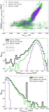 |
Fig. B.1 Impact of quality flags on the gspspec parameters. The data sets shown are the full (black), medium-quality (green), and best-quality (purple) samples. Top: Kiel diagram. Artifacts were progressively removed for more stringent selections. Middle: Calibrated metallicity distribution. The 16th, 50th, and 84th percentiles of each sample are shown in the colored text. The metal-poor tail was more heavily affected by the flags. Bottom: Distribution of surface gravity uncertainties. Only targets with small uncertainties survived the most stringent quality cuts. |
Appendix D Comparing extinction maps
Several extinction maps and catalogs have become available in the literature in recent years. In this section, we examine a number of them to decide which is more appropriate for our CMD analysis (Sect. 3). We limited our comparison to references that take into account the distances of stars, and thus did not include 2D maps such as the Gaia DR3 Total Galactic Extinction map (Delchambre et al. 2023), or the classical Schlegel et al. (1998) map (see also Schlafly & Finkbeiner 2011).
With this, the four references we consider are:
Vergely et al. (2022): we queried the extinction values using the EXPLORE website22 (see also Lallement et al. 2022), giving as input the Galactic longitudes, latitudes, and distances. This reference provides different maps with varying spatial extents and resolutions (namely 50pc, 25pc, and 10pc). We adopted the 50 pc resolution map, as the distances returned by its query did not saturate past 3 kpc (as was the case for the 25 pc and 10 pc maps). This decision does not impact our results, as the three maps provide extinctions in good agreement with each other for our targets (fractional differences of ≲ 5%). The extinction is reported in units of monochromatic extinction A0 (λ ≈ 550 nm). This map provides extinction values for 98.7% of our sample (194,299 stars), which includes every star in the CMD sample.
Bayestar19 (Green et al. 2019): we queried this map via the dustmaps package (Green 2018), using the same inputs as above. We only considered targets with the quality flags converged and reliable_dist set to True. The map reports reddening in units similar but not equal to E(B − V)23. We followed the dustmaps documentation24 and converted these reddenings to extinction AV by multiplying the Bayestar19 values by 2.742 (see also Table 6 in Schlafly & Finkbeiner (2011) with RV = 3.1). This map provides extinction values for 88.2% of our sample (173,630 stars).
Edenhofer et al. (2024): we queried this map using dustmaps and the same inputs as above. This reference also reports maps with varying resolutions and spatial extents (namely 1.25 kpc and 2 kpc). Both maps are in excellent agreement with each other (fractional difference of ≲ 1%). Given the distance distribution of our targets (see Sect. 2), we chose the map that extends out to 2 kpc. The map reports reddening in the units of Zhang et al. (2023), who in turn report their values in the same units as Bayestar19, and we thus applied the same multiplicative factor as above to convert them to AV. This map provides extinction values for 82.6% of our sample (162,561 stars).
Gaia DR3 gspphot (Creevey et al. 2023): we queried this catalog using the gaiadr3.astrophysical_parameters table. The extinction is reported in units of monochromatic extinction A0 (azero_gspphot), as well as in the Gaia bands. This catalog provides extinction values for 85.9% of our sample (169,047 stars).
We compare these references with each other in Figure D.1. We note that some of them are in slightly different units (AV vs. A0), but their differences are very small (e.g., Yamaguchi et al. 2024). Figure D.1 provides valuable insights:
The Bayestar19 values exhibits periodic gaps. This is due to this map being reported down to fewer decimal places than the others, hence producing quantized extinctions (appearing as horizontal/vertical stripes).
The gspphot values show a strong concentration of points near extinction ≈0 mag. Additionally, gspphot is the only reference with a significant fraction of its values around high extinctions (≳ 0.6 mag). Both of these features point to inaccuracies in the gspphot values, possibly due to the extinction-temperature degeneracy reported in Andrae et al. (2023a).
We find a good overall agreement between the Vergely et al. (2022), Edenhofer et al. (2024), and Bayestar19 maps, with all three of them showing a concentration of points around extinction ~ 0.2 mag. The comparison that more closely follows the 1:1 relation is that of Vergely et al. (2022) vs. Edenhofer et al. (2024).
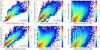 |
Fig. D.1 Comparison of the different extinction references considered in this work: Vergely et al. (2022), Edenhofer et al. (2024), Bayestar19, and gspphot. Each panel shows a 2D histogram of the extinction comparison between two references. The color bars indicate logarithmic density (with the same range for all panels), and the 1:1 line is shown in magenta. The number of stars in each plot is indicated in the bottom-right corner. Given that the Bayestar19 values are reported to fewer decimal places than the other references, the panels involving this map display horizontal/vertical stripes. The gspphot extinctions show the largest disagreement of all the references. For the CMD analysis, we adopted the Vergely et al. (2022) map as the source of extinctions. |
With this, we discarded the gspphot values as the source of extinction for our CMD analysis. Regarding the other three maps, they all have similar distributions, with median (standard deviation) values of 0.20 (0.14) mag for Vergely et al. (2022), 0.16 (0.13) mag for Edenhofer et al. (2024), and 0.24 (0.15) mag for Bayestar19. Thus, the Vergely et al. (2022) median is located halfway between the Edenhofer et al. (2024) and Bayestar19 values, with all three maps having almost identical standard deviations. For complementary discussions regarding extinction map comparisons, we refer to Van-Lane et al. (2024) (see their Appendix G.1).
In this work, whenever possible, we aim for homogeneity in the stellar properties. In this regard, the Vergely et al. (2022) map is the only one that provides extinction values for all our CMD targets. Given that this map is also in good agreement with Edenhofer et al. (2024) and Bayestar19, and that its distribution is an intermediate point between the other two, we adopted Vergely et al. (2022) as the source of extinction values throughout this paper.
Appendix E Characterization of the adopted extinction values
Following the discussion of Appendix D, Figure E.1 shows the distribution of extinction values from Vergely et al. (2022) for the CMD sample of Sect. 3. The histogram peaks around A0 ≈ 0.15 mag, with 16th and 84th percentiles of 0.12 to 0.32 mag.
To transform these monochromatic extinction values into the Gaia bands, we followed the (E)DR3 extinction law25. We mimicked the implementation of Godoy-Rivera et al. (2021a), updating the coefficients to those of Fitzpatrick et al. (2019). In brief, this is an iterative process that solves for km = Am/A0 (where m is one of the G, BP, or RP Gaia bands), as a function of de-reddened (BP − RP)0 color and A0. We followed the Gaia documentation and used different coefficients for the MS and the top of the HRD (transition at MG = 5 mag). We found km values from this method to be in good agreement with the values that can be obtained from gspphot (calculated from their Am and A0 values; see also dustapprox, Fouesneau et al. 2022). We also note that the coefficients are recommended to be used for colors inside the −0.06 ≤ (BP − RP)0 ≤ 2.5 mag range. However, when applying the coefficients for the entire color range of our sample, we observed a continuous behavior around these limits in the CMD and Hess diagram of Figure 2. Thus, given that the stars located outside the recommended color range are only 0.6% of the Kepler sample (1,211 targets), we chose to keep them in our catalog and leave it to the reader to decide whether to use them.
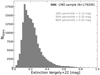 |
Fig. E.1 Distribution of the Vergely et al. (2022) monochromatic extinction values (A0) adopted for the CMD sample. The distribution peaks around ≈0.15 mag, with a median of ≈0.20 mag. |
With the above, we obtained star-by-star km values and calculated the extinction coefficients in the Gaia bands (i.e., Am = km × A0). The extinction errors were calculated with the analogous relation (σAm = km × σA0), using the σA0 values explained below. These AG, σAG, ABP, σABP, ARP, and σARP values were used to de-redden the photometry and propagate the errors in Sect. 3.3.
Regarding the error in the monochromatic extinction values, we consider both the random and systematic contributions. The errors reported by Vergely et al. (2022), which we take as the random errors, have a median of σA0,random/A0 ≈ 0.6%. These are significantly smaller than the values of the other extinction maps. The analogous values are ≈8.3% for Bayestar19, ≈9.6% for gspphot (or 17.3% when considering the × 1.8 inflation factor from Table 4 of Andrae et al. 2023a), and ≈5.6% for Edenhofer et al. (2024) (Phil Van-Lane, private communication). Thus, the random errors from Vergely et al. (2022) are probably underestimated.
To provide more realistic monochromatic extinction errors that include systematics (e.g., due to our choice of extinction map), we calculated a combined error as
![Mathematical equation: $\[\sigma_{A_0}=\sqrt{\left(\sigma_{A_{0, \text { random }}}\right)^2+\left(\sigma_{A_{0, \text { syst }}}\right)^2}.\]$](/articles/aa/full_html/2025/04/aa48735-23/aa48735-23-eq8.png) (E.1)
(E.1)
We used the difference between the Vergely et al. (2022) versus the Edenhofer et al. (2024) and Bayestar19 maps as a measure of this systematic error. The comparison yielded a combined median fractional difference of ≈19.1%. We approximate this to 20%, which we adopt as a global value for σA0,syt (i.e., σA0,sys = 0.2 × A0). Both A0 and σA0 values are reported in Table A.1.
Appendix F Coordinates of CMD regions
For reproducibility, we report the borders of the CMD regions defined throughout Sect. 3.4 as (color, magnitude) data points in Table F.1. We summarize these graphically in the left panel of Figure F.1 by showing the extent of the regions. In the right panel, we project these onto the Hess diagram of the CMD sample. As expected from the selection function of the Kepler mission, the region of dwarf stars concentrates the highest density (see also Table 1). Note that, for plotting purposes, the region plotted in the right panel is smaller than that of the left panel.
CMD regions.
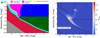 |
Fig. F.1 Illustration of the CMD regions presented in Sect. 3. The left panel displays the coordinates of the regions, and the right panel shows the Hess diagram of the CMD sample with the borders of the CMD regions overplotted. |
Appendix G Metallicity impact on suites of PARSEC models
Following Sect. 3.5.2, in Figure G.1 we replicated the suite of PARSEC models used to define the borders of the evolved CMD regions. We did this for three metallicity bins, namely [M/H] = −0.3, 0, and +0.3 dex, but kept the borders of the fiducial CMD regions at [M/H]=0 dex identical in all panels for visual reference. Although they vary as a function of CMD location, typical color and magnitude changes are of order ![Mathematical equation: $\[\frac{\mathrm{d}(B P{-}R P)_{0}}{\mathrm{~d}[\mathrm{M} / \mathrm{H}]} \sim 0.3\]$](/articles/aa/full_html/2025/04/aa48735-23/aa48735-23-eq9.png) and
and ![Mathematical equation: $\[\frac{\mathrm{d} M_{G_{0}}}{\mathrm{~d}[\mathrm{M} / \mathrm{H}]} \sim 0.9\]$](/articles/aa/full_html/2025/04/aa48735-23/aa48735-23-eq10.png) mag/dex (or 0.03 and 0.09 mag per +0.1 dex).
mag/dex (or 0.03 and 0.09 mag per +0.1 dex).
 |
Fig. G.1 Illustration of the metallicity-dependence of the evolved CMD regions, analogous to the top-left panel of Figure 3. From left to right, the panels show suites of PARSEC models at [M/H]=−0.3, 0, and +0.3 dex. The colors indicate the evolutionary stage for each metallicity bin. The borders used in the CMD classification of Sect. 3, calculated at [M/H]=0 dex, are shown as the thick grey lines in all panels. |
Appendix H Gaia NSS binary types and tables
The NSS binary types are encoded in a bit-condensed flag in the non_single_star column in the gaiadr3.gaia_source table. We have translated these to their plain meanings (astrometric, spectroscopic, eclipsing, and combinations thereof), and report them in the column “NSS Binary Type” of Table A.1. For example, a value of non_single_star = 3 is translated to 011 in binary notation, which in turn implies a “spectroscopic+astrometric” binary type.
Additionally, the Gaia DR3 NSS systems are reported in four tables, namely nss_two_body_orbit (TBO; systems with orbital parameters), nss_acceleration_astro (ACA; systems with acceleration solutions due to non-linear proper motions), nss_non_linear_spectro (NLS; spectroscopic binaries with long-period trend solutions), and nss_vim_fl (VIM; sources with variability induced movers). For further details, we refer to Gaia Collaboration (2023a). For completeness, we investigated the provenance of the 4,005 Kepler targets flagged as NSS in Sect. 4.3 by crossmatching with each of the four tables individually. We found 1,958 targets in the TBO, 1,866 targets in the ACA, 294 targets in the NLS, and 7 targets in the VIM. Some degree of overlap exists among them, with 71 targets appearing in both TBO and ACA, 1 target in both TBO and NLS, 3 targets in both TBO and VIM, and 45 targets in both ACA and NLS (with no other intersections found). For the targets classified as NSS by Gaia, we joined the 3-letter acronym of the tables they appear in, and created the column “NSS Tables” of Table A.1. For example, a star found in both TBO and ACA has NSS Tables = TboAca.
Appendix I Additional scrutiny of photometrically variable targets
We now expand on two of the variability classes discussed in Sect. 7, namely the stars with exoplanet transits (EP) and active galactic nuclei (AGN).
The Gaia photometry allows for the detection of exoplanet candidates via the transit method (Panahi et al. 2022; Rimoldini et al. 2023). We found 10 Kepler targets classified as EP. These correspond to KIC 4150804, KIC 5780885, KIC 9651668, KIC 9818381, KIC 10019708, KIC 10666592, KIC 10874614, KIC 11517719, KIC 11804465, and KIC 12019440. As per the Simbad database, all of these are reported in literature studies of exoplanet hosts (e.g., Su et al. 2022; Maxted 2023).
Additionally, we found 21 Kepler targets classified as AGN by Gaia DR3 (Carnerero et al. 2023). None of them pass our parallax SNR quality cut, as expected for extragalactic objects (e.g., Luri et al. 2018). We queried the Simbad database and found 13 of these targets reported in literature studies of Kepler AGNs and quasars (e.g., Scaringi et al. 2013; Dobrotka et al. 2017; Smith et al. 2018). For the remaining 8 targets, however, Simbad did not return any results. We list their IDs for interested readers: KIC 3730597, KIC 4356027, KIC 7729019, KIC 8160685, KIC 9339957, KIC 10070645, KIC 11862867, and KIC 11913354.
References
- Abdurro’uf, Accetta, K., Aerts, C., et al. 2022, ApJS, 259, 35 [NASA ADS] [CrossRef] [Google Scholar]
- Abril, J., Schmidtobreick, L., Ederoclite, A., & López-Sanjuan, C. 2020, MNRAS, 492, L40 [NASA ADS] [CrossRef] [Google Scholar]
- Andrae, R., Fouesneau, M., Sordo, R., et al. 2023a, A&A, 674, A27 [CrossRef] [EDP Sciences] [Google Scholar]
- Andrae, R., Rix, H.-W., & Chandra, V. 2023b, ApJS, 267, 8 [NASA ADS] [CrossRef] [Google Scholar]
- Bailer-Jones, C. A. L., Rybizki, J., Fouesneau, M., Mantelet, G., & Andrae, R. 2018, AJ, 156, 58 [Google Scholar]
- Bailer-Jones, C. A. L., Rybizki, J., Fouesneau, M., Demleitner, M., & Andrae, R. 2021, AJ, 161, 147 [Google Scholar]
- Ball, W. H., Triaud, A. H. M. J., Hatt, E., Nielsen, M. B., & Chaplin, W. J. 2023, MNRAS, 521, L1 [CrossRef] [Google Scholar]
- Batalha, N. M., Rowe, J. F., Bryson, S. T., et al. 2013, ApJS, 204, 24 [Google Scholar]
- Beck, P. G., Montalban, J., Kallinger, T., et al. 2012, Nature, 481, 55 [Google Scholar]
- Beck, P. G., Hambleton, K., Vos, J., et al. 2014, A&A, 564, A36 [NASA ADS] [CrossRef] [EDP Sciences] [Google Scholar]
- Beck, P. G., Mathur, S., Hambleton, K., et al. 2022, A&A, 667, A31 [NASA ADS] [CrossRef] [EDP Sciences] [Google Scholar]
- Beck, P. G., Grossmann, D. H., Steinwender, L., et al. 2024, A&A, 682, A7 [NASA ADS] [CrossRef] [EDP Sciences] [Google Scholar]
- Bedding, T. R., Mosser, B., Huber, D., et al. 2011, Nature, 471, 608 [Google Scholar]
- Belokurov, V., Penoyre, Z., Oh, S., et al. 2020, MNRAS, 496, 1922 [Google Scholar]
- Berger, T. A., Huber, D., Gaidos, E., & van Saders, J. L. 2018, ApJ, 866, 99 [NASA ADS] [CrossRef] [Google Scholar]
- Berger, T. A., Huber, D., van Saders, J. L., et al. 2020, AJ, 159, 280 [Google Scholar]
- Berger, T. A., Schlieder, J. E., & Huber, D. 2023, arXiv e-prints [arXiv:2301.11338] [Google Scholar]
- Bhalotia, V., Huber, D., van Saders, J. L., et al. 2024, ApJ, 970, 166 [Google Scholar]
- Borucki, W. J., Koch, D., Basri, G., et al. 2010, Science, 327, 977 [Google Scholar]
- Brandt, T. D. 2018, ApJS, 239, 31 [Google Scholar]
- Brandt, T. D. 2021, ApJS, 254, 42 [NASA ADS] [CrossRef] [Google Scholar]
- Bressan, A., Marigo, P., Girardi, L., et al. 2012, MNRAS, 427, 127 [NASA ADS] [CrossRef] [Google Scholar]
- Brown, T. M., Latham, D. W., Everett, M. E., & Esquerdo, G. A. 2011, AJ, 142, 112 [Google Scholar]
- Cantat-Gaudin, T., Jordi, C., Vallenari, A., et al. 2018, A&A, 618, A93 [NASA ADS] [CrossRef] [EDP Sciences] [Google Scholar]
- Canto Martins, B. L., Messias, Y. S., Arruda Gonçalves, M. I., et al. 2023, Nat. Astron., 7, 900 [Google Scholar]
- Cao, L., & Pinsonneault, M. H. 2022, MNRAS, 517, 2165 [NASA ADS] [CrossRef] [Google Scholar]
- Carnerero, M. I., Raiteri, C. M., Rimoldini, L., et al. 2023, A&A, 674, A24 [NASA ADS] [CrossRef] [EDP Sciences] [Google Scholar]
- Castro-Ginard, A., Penoyre, Z., Casey, A. R., et al. 2024, A&A, 688, A1 [NASA ADS] [CrossRef] [EDP Sciences] [Google Scholar]
- Chambers, K. C., Magnier, E. A., Metcalfe, N., et al. 2016, arXiv e-prints [arXiv:1612.05560] [Google Scholar]
- Chen, Y., Girardi, L., Bressan, A., et al. 2014, MNRAS, 444, 2525 [Google Scholar]
- Choi, J., Dotter, A., Conroy, C., et al. 2016, ApJ, 823, 102 [Google Scholar]
- Clementini, G., Ripepi, V., Garofalo, A., et al. 2023, A&A, 674, A18 [NASA ADS] [CrossRef] [EDP Sciences] [Google Scholar]
- Coughlin, J. L., López-Morales, M., Harrison, T. E., Ule, N., & Hoffman, D. I. 2011, AJ, 141, 78 [NASA ADS] [CrossRef] [Google Scholar]
- Creevey, O. L., Sordo, R., Pailler, F., et al. 2023, A&A, 674, A26 [NASA ADS] [CrossRef] [EDP Sciences] [Google Scholar]
- Curtis, J. L., Agüeros, M. A., Douglas, S. T., & Meibom, S. 2019, ApJ, 879, 49 [Google Scholar]
- Cutri, R. M., Skrutskie, M. F., van Dyk, S., et al. 2003, VizieR Online Data Catalog: 2MASS All-Sky Catalog of Point Sources (Cutri+ 2003), VizieR On-line Data Catalog: II/246. Originally published in: 2003yCat.2246....0C [Google Scholar]
- De Angeli, F., Weiler, M., Montegriffo, P., et al. 2023, A&A, 674, A2 [NASA ADS] [CrossRef] [EDP Sciences] [Google Scholar]
- Delchambre, L., Bailer-Jones, C. A. L., Bellas-Velidis, I., et al. 2023, A&A, 674, A31 [NASA ADS] [CrossRef] [EDP Sciences] [Google Scholar]
- Distefano, E., Lanzafame, A. C., Brugaletta, E., et al. 2023, A&A, 674, A20 [NASA ADS] [CrossRef] [EDP Sciences] [Google Scholar]
- Dobrotka, A., Antonuccio-Delogu, V., & Bajčičáková, I. 2017, MNRAS, 470, 2439 [NASA ADS] [CrossRef] [Google Scholar]
- Donada, J., Anders, F., Jordi, C., et al. 2023, A&A, 675, A89 [NASA ADS] [CrossRef] [EDP Sciences] [Google Scholar]
- Dong, S., Zheng, Z., Zhu, Z., et al. 2014, ApJ, 789, L3 [NASA ADS] [CrossRef] [Google Scholar]
- Dotter, A., Chaboyer, B., Jevremović, D., et al. 2008, ApJS, 178, 89 [Google Scholar]
- Doyle, T. F., Howell, S. B., Petit, V., & Lépine, S. 2017, MNRAS, 464, 3464 [Google Scholar]
- Dubus, G., & Babusiaux, C. 2024, A&A, 683, A247 [NASA ADS] [CrossRef] [EDP Sciences] [Google Scholar]
- Duchêne, G., & Kraus, A. 2013, ARA&A, 51, 269 [Google Scholar]
- Duquennoy, A., & Mayor, M. 1991, A&A, 248, 485 [NASA ADS] [Google Scholar]
- Edenhofer, G., Zucker, C., Frank, P., et al. 2024, A&A, 685, A82 [NASA ADS] [CrossRef] [EDP Sciences] [Google Scholar]
- El-Badry, K., Rix, H.-W., & Heintz, T. M. 2021, MNRAS, 506, 2269 [NASA ADS] [CrossRef] [Google Scholar]
- ESA 1997, ESA Special Publication, 1200, The HIPPARCOS and TYCHO Catalogues. Astrometric and Photometric Star Catalogues Derived from the ESA HIPPARCOS Space Astrometry Mission (Noordwijk, The Netherlands: ESA Publications Division) [Google Scholar]
- Escorza, A., & De Rosa, R. J. 2023, A&A, 671, A97 [NASA ADS] [CrossRef] [EDP Sciences] [Google Scholar]
- Eyer, L., Audard, M., Holl, B., et al. 2023, A&A, 674, A13 [NASA ADS] [CrossRef] [EDP Sciences] [Google Scholar]
- Fabricius, C., Luri, X., Arenou, F., et al. 2021, A&A, 649, A5 [NASA ADS] [CrossRef] [EDP Sciences] [Google Scholar]
- Fitton, S., Tofflemire, B. M., & Kraus, A. L. 2022, Res. Notes Am. Astron. Soc., 6, 18 [Google Scholar]
- Fitzpatrick, E. L., Massa, D., Gordon, K. D., Bohlin, R., & Clayton, G. C. 2019, ApJ, 886, 108 [Google Scholar]
- Fouesneau, M., Andrae, R., Sordo, R., & Dharmawardena, T. 2022, dustapprox, https://github.com/mfouesneau/dustapprox [Google Scholar]
- Fouesneau, M., Frémat, Y., Andrae, R., et al. 2023, A&A, 674, A28 [NASA ADS] [CrossRef] [EDP Sciences] [Google Scholar]
- Frasca, A., Molenda-Żakowicz, J., De Cat, P., et al. 2016, A&A, 594, A39 [CrossRef] [EDP Sciences] [Google Scholar]
- Gaia Collaboration (Prusti, T., et al.) 2016, A&A, 595, A1 [NASA ADS] [CrossRef] [EDP Sciences] [Google Scholar]
- Gaia Collaboration (Babusiaux, C., et al.) 2018a, A&A, 616, A10 [NASA ADS] [CrossRef] [EDP Sciences] [Google Scholar]
- Gaia Collaboration (Brown, A. G. A., et al.) 2018b, A&A, 616, A1 [NASA ADS] [CrossRef] [EDP Sciences] [Google Scholar]
- Gaia Collaboration (Eyer, L., et al.) 2019, A&A, 623, A110 [NASA ADS] [CrossRef] [EDP Sciences] [Google Scholar]
- Gaia Collaboration (Brown, A. G. A., et al.) 2021, A&A, 649, A1 [NASA ADS] [CrossRef] [EDP Sciences] [Google Scholar]
- Gaia Collaboration (Arenou, F., et al.) 2023a, A&A, 674, A34 [CrossRef] [EDP Sciences] [Google Scholar]
- Gaia Collaboration (Creevey, O. L., et al.) 2023b, A&A, 674, A39 [CrossRef] [EDP Sciences] [Google Scholar]
- Gaia Collaboration (Trabucchi, M., et al.) 2023c, A&A, 680, A36 [NASA ADS] [CrossRef] [EDP Sciences] [Google Scholar]
- Gaia Collaboration (Vallenari, A., et al.) 2023d, A&A, 674, A1 [NASA ADS] [CrossRef] [EDP Sciences] [Google Scholar]
- García, R. A., Ceillier, T., Salabert, D., et al. 2014, A&A, 572, A34 [NASA ADS] [CrossRef] [EDP Sciences] [Google Scholar]
- García, R. A., Gourvès, C., Santos, A. R. G., et al. 2023, A&A, 679, L12 [NASA ADS] [CrossRef] [EDP Sciences] [Google Scholar]
- Gaulme, P., McKeever, J., Jackiewicz, J., et al. 2016, ApJ, 832, 121 [NASA ADS] [CrossRef] [Google Scholar]
- Gavras, P., Rimoldini, L., Nienartowicz, K., et al. 2023, A&A, 674, A22 [NASA ADS] [CrossRef] [EDP Sciences] [Google Scholar]
- Gehan, C., Gaulme, P., & Yu, J. 2022, A&A, 668, A116 [NASA ADS] [CrossRef] [EDP Sciences] [Google Scholar]
- Gehan, C., Godoy-Rivera, D., & Gaulme, P. 2024, A&A, 686, A93 [NASA ADS] [CrossRef] [EDP Sciences] [Google Scholar]
- Gentile Fusillo, N. P., Tremblay, P. E., Cukanovaite, E., et al. 2021, MNRAS, 508, 3877 [NASA ADS] [CrossRef] [Google Scholar]
- Godoy-Rivera, D., & Chanamé, J. 2018, MNRAS, 479, 4440 [Google Scholar]
- Godoy-Rivera, D., Pinsonneault, M. H., & Rebull, L. M. 2021a, ApJS, 257, 46 [CrossRef] [Google Scholar]
- Godoy-Rivera, D., Tayar, J., Pinsonneault, M. H., et al. 2021b, ApJ, 915, 19 [NASA ADS] [CrossRef] [Google Scholar]
- Gordon, T. A., Davenport, J. R. A., Angus, R., et al. 2021, ApJ, 913, 70 [Google Scholar]
- Gosset, E., Damerdji, Y., Morel, T., et al. 2025, A&A, 693, A124 [NASA ADS] [CrossRef] [EDP Sciences] [Google Scholar]
- Green, G. 2018, J. Open Source Softw., 3, 695 [NASA ADS] [CrossRef] [Google Scholar]
- Green, G. M., Schlafly, E., Zucker, C., Speagle, J. S., & Finkbeiner, D. 2019, ApJ, 887, 93 [NASA ADS] [CrossRef] [Google Scholar]
- Grossmann, D. H., Beck, P. G., Mathur, S., et al. 2025, A&A, 696, A42 [NASA ADS] [CrossRef] [EDP Sciences] [Google Scholar]
- Halbwachs, J.-L., Pourbaix, D., Arenou, F., et al. 2023, A&A, 674, A9 [NASA ADS] [CrossRef] [EDP Sciences] [Google Scholar]
- Hall, O. J., Davies, G. R., van Saders, J., et al. 2021, Nat. Astron., 5, 707 [NASA ADS] [CrossRef] [Google Scholar]
- Hambleton, K. M., Kurtz, D. W., Prša, A., et al. 2013, MNRAS, 434, 925 [Google Scholar]
- Hambleton, K., Kurtz, D. W., Prša, A., et al. 2016, MNRAS, 463, 1199 [Google Scholar]
- Hambleton, K., Fuller, J., Thompson, S., et al. 2018, MNRAS, 473, 5165 [Google Scholar]
- Hey, D., & Aerts, C. 2024, A&A, 688, A93 [NASA ADS] [CrossRef] [EDP Sciences] [Google Scholar]
- Hidalgo, S. L., Pietrinferni, A., Cassisi, S., et al. 2018, ApJ, 856, 125 [Google Scholar]
- Holl, B., Sozzetti, A., Sahlmann, J., et al. 2023, A&A, 674, A10 [NASA ADS] [CrossRef] [EDP Sciences] [Google Scholar]
- Howard, A. W., Marcy, G. W., Bryson, S. T., et al. 2012, ApJS, 201, 15 [Google Scholar]
- Howell, S. B., Sobeck, C., Haas, M., et al. 2014, PASP, 126, 398 [Google Scholar]
- Huber, D., Silva Aguirre, V., Matthews, J. M., et al. 2014, ApJS, 211, 2 [NASA ADS] [CrossRef] [Google Scholar]
- Hurley, J., & Tout, C. A. 1998, MNRAS, 300, 977 [CrossRef] [Google Scholar]
- Kamai, I., & Perets, H. B. 2025, AJ, 169, 59 [Google Scholar]
- Katz, D., Sartoretti, P., Guerrier, A., et al. 2023, A&A, 674, A5 [NASA ADS] [CrossRef] [EDP Sciences] [Google Scholar]
- Kervella, P., Arenou, F., & Thévenin, F. 2022, A&A, 657, A7 [NASA ADS] [CrossRef] [EDP Sciences] [Google Scholar]
- Khalatyan, A., Anders, F., Chiappini, C., et al. 2024, A&A, 691, A98 [NASA ADS] [CrossRef] [EDP Sciences] [Google Scholar]
- Kirk, B., Conroy, K., Prša, A., et al. 2016, AJ, 151, 68 [Google Scholar]
- Kuhn, M. A., Hillenbrand, L. A., Sills, A., Feigelson, E. D., & Getman, K. V. 2019, ApJ, 870, 32 [CrossRef] [Google Scholar]
- Lallement, R., Vergely, J. L., Babusiaux, C., & Cox, N. L. J. 2022, A&A, 661, A147 [NASA ADS] [CrossRef] [EDP Sciences] [Google Scholar]
- Lebzelter, T., Mowlavi, N., Lecoeur-Taibi, I., et al. 2023, A&A, 674, A15 [NASA ADS] [CrossRef] [EDP Sciences] [Google Scholar]
- Lewis, H. M., Anguiano, B., Majewski, S. R., et al. 2022, MNRAS, 509, 3355 [Google Scholar]
- Li, L., Shao, Z., Li, Z.-Z., et al. 2020, ApJ, 901, 49 [Google Scholar]
- Li, G., Deheuvels, S., Ballot, J., & Lignières, F. 2022, Nature, 610, 43 [NASA ADS] [CrossRef] [Google Scholar]
- Lindegren, L. 2018, Technical Note gAIA-C3-TN-LU-LL-124, http://www.rssd.esa.int/doc_fetch.php?id=3757412 [Google Scholar]
- Lindegren, L., Hernández, J., Bombrun, A., et al. 2018, A&A, 616, A2 [NASA ADS] [CrossRef] [EDP Sciences] [Google Scholar]
- Lindegren, L., Bastian, U., Biermann, M., et al. 2021a, A&A, 649, A4 [EDP Sciences] [Google Scholar]
- Lindegren, L., Klioner, S. A., Hernández, J., et al. 2021b, A&A, 649, A2 [EDP Sciences] [Google Scholar]
- Long, L., Bi, S., Zhang, J., et al. 2023, ApJS, 268, 30 [Google Scholar]
- Lu, Y., Benomar, O., Kamiaka, S., & Suto, Y. 2022, ApJ, 941, 175 [NASA ADS] [CrossRef] [Google Scholar]
- Luri, X., Brown, A. G. A., Sarro, L. M., et al. 2018, A&A, 616, A9 [NASA ADS] [CrossRef] [EDP Sciences] [Google Scholar]
- Lurie, J. C., Vyhmeister, K., Hawley, S. L., et al. 2017, AJ, 154, 250 [Google Scholar]
- Maíz Apellániz, J., & Weiler, M. 2024, arXiv e-prints [arXiv:2407.21388] [Google Scholar]
- Maoz, D., Mazeh, T., & McQuillan, A. 2015, MNRAS, 447, 1749 [NASA ADS] [CrossRef] [Google Scholar]
- Martin, D. V. 2018, in Handbook of Exoplanets, eds. H. J. Deeg, & J. A. Belmonte (Berlin: Springer), 156 [Google Scholar]
- Martínez-Palomera, J., Hedges, C., & Dotson, J. 2023, AJ, 166, 265 [CrossRef] [Google Scholar]
- Marton, G., Ábrahám, P., Rimoldini, L., et al. 2023, A&A, 674, A21 [NASA ADS] [CrossRef] [EDP Sciences] [Google Scholar]
- Mason, B. D., Wycoff, G. L., Hartkopf, W. I., Douglass, G. G., & Worley, C. E. 2001, AJ, 122, 3466 [Google Scholar]
- Mathur, S., García, R. A., Huber, D., et al. 2016, ApJ, 827, 50 [NASA ADS] [CrossRef] [Google Scholar]
- Mathur, S., Huber, D., Batalha, N. M., et al. 2017, ApJS, 229, 30 [NASA ADS] [CrossRef] [Google Scholar]
- Mathur, S., García, R. A., Breton, S., et al. 2022, A&A, 657, A31 [NASA ADS] [CrossRef] [EDP Sciences] [Google Scholar]
- Mathur, S., Claytor, Z. R., Santos, Â. R. G., et al. 2023, ApJ, 952, 131 [NASA ADS] [CrossRef] [Google Scholar]
- Maxted, P. F. L. 2023, MNRAS, 519, 3723 [NASA ADS] [CrossRef] [Google Scholar]
- McQuillan, A., Mazeh, T., & Aigrain, S. 2013, ApJ, 775, L11 [Google Scholar]
- McQuillan, A., Mazeh, T., & Aigrain, S. 2014, ApJS, 211, 24 [Google Scholar]
- Merc, J., Gális, R., Kára, J., Wolf, M., & Vrašt’ák, M. 2020, MNRAS, 499, 2116 [NASA ADS] [CrossRef] [Google Scholar]
- Merc, J., Gális, R., Wolf, M., et al. 2021, MNRAS, 506, 4151 [NASA ADS] [CrossRef] [Google Scholar]
- Messias, Y. S., de Oliveira, L. L. A., Gomes, R. L., et al. 2022, ApJ, 930, L23 [NASA ADS] [CrossRef] [Google Scholar]
- Miglio, A., Chiappini, C., Morel, T., et al. 2013, MNRAS, 429, 423 [Google Scholar]
- Mikkola, D., McMillan, P. J., & Hobbs, D. 2023, MNRAS, 519, 1989 [Google Scholar]
- Montegriffo, P., De Angeli, F., Andrae, R., et al. 2023, A&A, 674, A3 [NASA ADS] [CrossRef] [EDP Sciences] [Google Scholar]
- Mosser, B., Goupil, M. J., Belkacem, K., et al. 2012, A&A, 548, A10 [NASA ADS] [CrossRef] [EDP Sciences] [Google Scholar]
- Mowlavi, N., Holl, B., Lecoeur-Taïbi, I., et al. 2023, A&A, 674, A16 [NASA ADS] [CrossRef] [EDP Sciences] [Google Scholar]
- Munari, U. 2019, arXiv e-prints [arXiv:1909.01389] [Google Scholar]
- Nguyen, C. T., Costa, G., Girardi, L., et al. 2022, A&A, 665, A126 [NASA ADS] [CrossRef] [EDP Sciences] [Google Scholar]
- Panahi, A., Zucker, S., Clementini, G., et al. 2022, A&A, 663, A101 [NASA ADS] [CrossRef] [EDP Sciences] [Google Scholar]
- Pang, X., Wang, Y., Tang, S.-Y., et al. 2023, AJ, 166, 110 [NASA ADS] [CrossRef] [Google Scholar]
- Patton, R. A., Pinsonneault, M. H., Cao, L., et al. 2024, MNRAS, 528, 3232 [NASA ADS] [CrossRef] [Google Scholar]
- Pecaut, M. J., & Mamajek, E. E. 2013, ApJS, 208, 9 [Google Scholar]
- Penoyre, Z., Belokurov, V., Wyn Evans, N., Everall, A., & Koposov, S. E. 2020, MNRAS, 495, 321 [NASA ADS] [CrossRef] [Google Scholar]
- Penoyre, Z., Belokurov, V., & Evans, N. W. 2022, MNRAS, 513, 2437 [NASA ADS] [CrossRef] [Google Scholar]
- Pinsonneault, M. H., Elsworth, Y., Epstein, C., et al. 2014, ApJS, 215, 19 [Google Scholar]
- Pinsonneault, M. H., Elsworth, Y. P., Tayar, J., et al. 2018, ApJS, 239, 32 [Google Scholar]
- Pinsonneault, M. H., Zinn, J. C., Tayar, J., et al. 2025, ApJS, 276, 69 [NASA ADS] [CrossRef] [Google Scholar]
- Pourbaix, D., Tokovinin, A. A., Batten, A. H., et al. 2004, A&A, 424, 727 [NASA ADS] [CrossRef] [EDP Sciences] [Google Scholar]
- Prša, A. 2018, Modeling and Analysis of Eclipsing Binary Stars; The Theory and Design Principles of PHOEBE (Bristol: IOP Publishing Limited) [Google Scholar]
- Prša, A., Batalha, N., Slawson, R. W., et al. 2011, AJ, 141, 83 [Google Scholar]
- Raghavan, D., McAlister, H. A., Henry, T. J., et al. 2010, ApJS, 190, 1 [Google Scholar]
- Recio-Blanco, A., de Laverny, P., Palicio, P. A., et al. 2023, A&A, 674, A29 [NASA ADS] [CrossRef] [EDP Sciences] [Google Scholar]
- Reinhold, T., Shapiro, A. I., Solanki, S. K., & Basri, G. 2023, A&A, 678, A24 [NASA ADS] [CrossRef] [EDP Sciences] [Google Scholar]
- Ren, A., Fu, J., De Cat, P., et al. 2016, ApJS, 225, 28 [NASA ADS] [CrossRef] [Google Scholar]
- Riello, M., De Angeli, F., Evans, D. W., et al. 2021, A&A, 649, A3 [NASA ADS] [CrossRef] [EDP Sciences] [Google Scholar]
- Rimoldini, L., Holl, B., Gavras, P., et al. 2023, A&A, 674, A14 [NASA ADS] [CrossRef] [EDP Sciences] [Google Scholar]
- Ripepi, V., Clementini, G., Molinaro, R., et al. 2023, A&A, 674, A17 [NASA ADS] [CrossRef] [EDP Sciences] [Google Scholar]
- Roelens, M., Eyer, L., Mowlavi, N., et al. 2017, MNRAS, 472, 3230 [CrossRef] [Google Scholar]
- Roelens, M., Eyer, L., Mowlavi, N., et al. 2018, A&A, 620, A197 [NASA ADS] [CrossRef] [EDP Sciences] [Google Scholar]
- Sandquist, E. L., Jessen-Hansen, J., Shetrone, M. D., et al. 2016, ApJ, 831, 11 [Google Scholar]
- Santos, A. R. G., García, R. A., Mathur, S., et al. 2019, ApJS, 244, 21 [Google Scholar]
- Santos, A. R. G., Breton, S. N., Mathur, S., & García, R. A. 2021, ApJS, 255, 17 [NASA ADS] [CrossRef] [Google Scholar]
- Santos, A. R. G., Mathur, S., García, R. A., et al. 2023, A&A, 672, A56 [NASA ADS] [CrossRef] [EDP Sciences] [Google Scholar]
- Santos, Â. R. G., Godoy-Rivera, D., Finley, A. J., et al. 2024, Front. Astron. Space Sci., 11, 1356379 [NASA ADS] [CrossRef] [Google Scholar]
- Scaringi, S., Groot, P. J., Verbeek, K., et al. 2013, MNRAS, 428, 2207 [NASA ADS] [CrossRef] [Google Scholar]
- Schlafly, E. F., & Finkbeiner, D. P. 2011, ApJ, 737, 103 [Google Scholar]
- Schlegel, D. J., Finkbeiner, D. P., & Davis, M. 1998, ApJ, 500, 525 [Google Scholar]
- Schonhut-Stasik, J., & Stassun, K. 2023, Res. Notes Am. Astron. Soc., 7, 18 [Google Scholar]
- Serenelli, A., Johnson, J., Huber, D., et al. 2017, ApJS, 233, 23 [Google Scholar]
- Serenelli, A., Weiss, A., Aerts, C., et al. 2021, A&A Rev., 29, 4 [NASA ADS] [CrossRef] [Google Scholar]
- Silva Aguirre, V., Lund, M. N., Antia, H. M., et al. 2017, ApJ, 835, 173 [Google Scholar]
- Silva-Beyer, J., Godoy-Rivera, D., & Chanamé, J. 2023, MNRAS, 523, 5947 [NASA ADS] [CrossRef] [Google Scholar]
- Simonian, G. V. A., Pinsonneault, M. H., & Terndrup, D. M. 2019, ApJ, 871, 174 [Google Scholar]
- Simonian, G. V. A., Pinsonneault, M. H., Terndrup, D. M., & van Saders, J. L. 2020, ApJ, 898, 76 [NASA ADS] [CrossRef] [Google Scholar]
- Skrutskie, M. F., Cutri, R. M., Stiening, R., et al. 2006, AJ, 131, 1163 [NASA ADS] [CrossRef] [Google Scholar]
- Smith, K. L., Mushotzky, R. F., Boyd, P. T., et al. 2018, ApJ, 857, 141 [NASA ADS] [CrossRef] [Google Scholar]
- Stassun, K. G., Oelkers, R. J., Pepper, J., et al. 2018, AJ, 156, 102 [Google Scholar]
- Stassun, K. G., Oelkers, R. J., Paegert, M., et al. 2019, AJ, 158, 138 [Google Scholar]
- Stauffer, J., Rebull, L. M., Cody, A. M., et al. 2018, AJ, 156, 275 [NASA ADS] [CrossRef] [Google Scholar]
- Su, T., Zhang, L.-y., Long, L., et al. 2022, ApJS, 261, 26 [NASA ADS] [CrossRef] [Google Scholar]
- Taylor, M. B. 2005, ASP Conf. Ser., 347, 29 [Google Scholar]
- Torres, G., Andersen, J., & Giménez, A. 2010, A&A Rev., 18, 67 [Google Scholar]
- Van-Lane, P. R., Speagle, J. S., Eadie, G. M., et al. 2024, arXiv e-prints [arXiv:2412.12244] [Google Scholar]
- van Saders, J. L., Ceillier, T., Metcalfe, T. S., et al. 2016, Nature, 529, 181 [Google Scholar]
- Vergely, J. L., Lallement, R., & Cox, N. L. J. 2022, A&A, 664, A174 [NASA ADS] [CrossRef] [EDP Sciences] [Google Scholar]
- Vrard, M., Cunha, M. S., Bossini, D., et al. 2022, Nat. Commun., 13, 7553 [CrossRef] [Google Scholar]
- Wolniewicz, L. M., Berger, T. A., & Huber, D. 2021, AJ, 161, 231 [Google Scholar]
- Wright, E. L., Eisenhardt, P. R. M., Mainzer, A. K., et al. 2010, AJ, 140, 1868 [Google Scholar]
- Yamaguchi, N., El-Badry, K., Rees, N. R., et al. 2024, PASP, 136, 084202 [Google Scholar]
- Yu, J., Huber, D., Bedding, T. R., et al. 2018, ApJS, 236, 42 [NASA ADS] [CrossRef] [Google Scholar]
- Yu, J., Bedding, T. R., Stello, D., et al. 2020, MNRAS, 493, 1388 [Google Scholar]
- Zhang, X., Green, G. M., & Rix, H.-W. 2023, MNRAS, 524, 1855 [NASA ADS] [CrossRef] [Google Scholar]
- Zhou, A.-Y. 2024, Res. Notes Am. Astron. Soc., 8, 110 [Google Scholar]
- Ziegler, C., Tokovinin, A., Briceño, C., et al. 2020, AJ, 159, 19 [Google Scholar]
- Zong, W., Fu, J.-N., De Cat, P., et al. 2018, ApJS, 238, 30 [NASA ADS] [CrossRef] [Google Scholar]
- Zwintz, K., & Steindl, T. 2022, Front. Astron. Space Sci., 9, 914738 [NASA ADS] [CrossRef] [Google Scholar]
https://gaia-kepler.fun/. Download date = 13/06/2024.
Queried with the gaiadr3_zeropoint tool hosted at https://gitlab.com/icc-ub/public/gaiadr3_zeropoint
The different evolutionary phases in the PARSEC models are identified by combining interior physics and Hertzsprung–Russell diagram (HRD) morphology (Bressan et al. 2012). They are specified via the label column (1 = MS, 2 = SGB, 3 = RGB, among others).
Catalog version V1.0, containing ≈124 million rows.
For practicality, when comparing with the FLAME labels, we grouped our CMD categories as main sequence = (Dwarf+Photometric Binary+Uncertain MS), subgiant = (Subgiant+Overlap Dwarf/Subgiant), and red giants = (Giant Branch).
From the gaiadr3.gaia_source table, we used the RV variability selection criteria rv_nb_transits ≥ 10, 3900 K ≤ rv_template_teff ≤ 8000 K, rv_chisq_pvalue ≤ 0.01, and rv_renormalised_gof > 4 (see Section 3.7 of Katz et al. 2023).
Note that this catalog includes several classes of systems (e.g., with tertiary eclipses, with changing eclipse depths, and heartbeat systems, among others). We included the full table in our crossmatch. The catalog is hosted at https://keplerebs.villanova.edu/
Kepler EB Catalog, Third Revision, version = 08/08/2019.
SB9 catalog version = 22/04/2024.
NEA confirmed exoplanets version = 01/06/2025.
WDS catalog version = 02/12/2024.
Created with the venny4py tool.
These can be found by requiring Flag ΔDM = TRUE and measured values for NEA sy_snum. Of the 52 targets, 46 have PCMD < 0.70, and 6 have PCMD ≥ 0.70.
Note that the ACV|CP|MCP|ROAM|ROAP|SXARI class is abbreviated to ACV|CP| . . . | SXARI in Figure 10 for plotting purposes (following Table 1 in Rimoldini et al. 2023).
For metallicity, we adopted the calibration with respect to the literature sample over the open cluster sample, as the latter is restricted to a more metal-rich regime.
All Tables
All Figures
|
Fig. 1 Characterization of the Kepler targets. Top-left: distribution of apparent Gaia G-band magnitudes. The targets are mostly concentrated in the 10 < G < 16 mag range. Top-right: distribution of Gaia distances. The distribution peaks around ~1 kpc. Bottom-left: distribution of RUWE values, with the vertical lines indicating RUWE = 1.0 (green), 1.2 (cyan), and 1.4 (red). From this, RUWE binaries are later identified in Sect. 4. Bottom-right: distribution of calibrated metallicity values, for the subsample with best-quality gspspec data. The distribution peaks around [M/H] = 0 dex, in agreement with the literature. |
| In the text | |
|
Fig. 2 Absolute and de-reddened Gaia CMD of the Kepler targets. Top-left: CMD sample described in Sect. 3. The purple marker illustrates the median error bars. Top-right: Hess diagram of the CMD sample. Bottom: CMD sample, with the stars color-coded according to the CMD categories we define in Sect. 3. The black lines illustrate the borders of the CMD regions. |
| In the text | |
|
Fig. 3 Characterization of the CMD regions presented in Sect. 3. The top-left panel shows the suite of PARSEC models we used to define the upper-CMD regions, and the projections of these onto the Hess diagram are displayed in the top-right panel. The bottom-left panel shows the Hess diagram and borders of the lower-CMD regions. The bottom-right panel shows the distribution of ΔMG0 values we used to define the Photometric Binary region. |
| In the text | |
|
Fig. 4 Validation of the CMD categories via the Monte Carlo method presented in Sect. 3.6. Top: Logarithmic distribution of the probability of CMD category parameter, PCMD. The filled histogram represents the fiducial simulation (Sect. 3.5.1), while the open histogram represents the simulation that includes metallicity effects (Sect. 3.5.2). Bottom: CMD projection color-coded by the fiducial PCMD values. Most of the stars have high PCMD values, indicating that their assigned CMD categories are reliable. Targets with low PCMD values are located near the boundaries of the CMD regions (see bottom panel of Figure 2), and their CMD categories are consequently less reliable. |
| In the text | |
|
Fig. 5 Metallicity impact on the CMD classification. The blue and red points show, respectively, the metal-poor and metal-rich tails (beyond 2σ) of the Andrae et al. (2023b) metallicity distribution. Our CMD classification loses accuracy towards extreme-metallicity values, and this effect is enhanced in certain regions of the CMD. |
| In the text | |
|
Fig. 6 Characterization of the binary categories defined in Sect. 4. The panels display the CMD projection of the RUWE, RV Variable, NSS, Kepler + Gaia EB, SB9 + NEA + HGCA, and WDS binary samples, respectively. In all the CMDs, we show the separation between MS and evolved stars as guidance (dashed fuchsia line). The number of systems in each category is summarized in the bottom-right corner. The CMD projections help to illustrate the selection effects of each category (see Sect. 4 for details). |
| In the text | |
|
Fig. 7 Comparison of the four most numerous binary categories. Top: distribution of apparent G-band magnitudes. The RV Variable and RUWE binary candidates are concentrated at the bright and faint limits of the Kepler sample, respectively. Bottom: Venn diagram. While some categories show a moderate degree of overlap (e.g., RV Variable and NSS), others do not (e.g., RUWE). |
| In the text | |
|
Fig. 8 Astrometric comparison between Gaia DR3 and DR2 from Sect. 5. Top: 2D histogram of the distance comparison. Most targets closely follow the 1:1 relation. Middle: Distribution of the distance modulus difference (in the sense of DR3 minus DR2). Stars are heavily centered around ΔDM = 0, but outliers outside the 1.5:1 and 1:1.5 relations are selected for further inspection (blue and red samples). Bottom: CMD projection of the ΔDM outliers, with their DR3 and DR2 positions shown in the green squares and yellow crosses, respectively. The astrometric differences can drive important CMD changes, thus modifying the derived stellar properties. |
| In the text | |
|
Fig. 9 Gaia DR3 analysis of the misclassified stars identified by Mathur et al. (2016) from Sect. 6. Top: distance comparison. The sample was split between targets inside (orange) and outside (green) the 2:1 and 1:2 lines. Middle: Gaia CMD projection. The targets with large distance discrepancies (green) appear predominantly as MS stars in Gaia, and most of them have crowding or blending flags (overplotted blue) in Mathur et al. (2016). Bottom: ΔG vs. Δθ diagram (and marginalized distributions) of the stars’ neighborhoods. The targets outside the distance range have more bright nearby neighbors than the targets inside the distance range, and thus the former are more prone to having contaminated Kepler light curves than the latter. |
| In the text | |
|
Fig. 10 Photometric variability analysis of the Kepler targets from Sect. 7. Top: bar chart of the 19 classes of variable sources found in Gaia DR3. The text inside the bars lists the number of targets in each class (with the size of the CMD subset shown in parenthesis). Middle: CMD projection of the variable sources with classifications. Targets are color-coded following the bars in the top panel, and the symbol size increases for smaller samples. The full CMD sample (grey) is shown for reference in the background. The interpretations of the CMD locations are greatly benefited by the variability classifications in Gaia DR3. Bottom: CMD projection of the “Gaia short-timescale variable only” targets (black squares). A significant fraction of them were found to be Kepler eclipsing binaries (cyan crosses). |
| In the text | |
|
Fig. B.1 Impact of quality flags on the gspspec parameters. The data sets shown are the full (black), medium-quality (green), and best-quality (purple) samples. Top: Kiel diagram. Artifacts were progressively removed for more stringent selections. Middle: Calibrated metallicity distribution. The 16th, 50th, and 84th percentiles of each sample are shown in the colored text. The metal-poor tail was more heavily affected by the flags. Bottom: Distribution of surface gravity uncertainties. Only targets with small uncertainties survived the most stringent quality cuts. |
| In the text | |
|
Fig. D.1 Comparison of the different extinction references considered in this work: Vergely et al. (2022), Edenhofer et al. (2024), Bayestar19, and gspphot. Each panel shows a 2D histogram of the extinction comparison between two references. The color bars indicate logarithmic density (with the same range for all panels), and the 1:1 line is shown in magenta. The number of stars in each plot is indicated in the bottom-right corner. Given that the Bayestar19 values are reported to fewer decimal places than the other references, the panels involving this map display horizontal/vertical stripes. The gspphot extinctions show the largest disagreement of all the references. For the CMD analysis, we adopted the Vergely et al. (2022) map as the source of extinctions. |
| In the text | |
|
Fig. E.1 Distribution of the Vergely et al. (2022) monochromatic extinction values (A0) adopted for the CMD sample. The distribution peaks around ≈0.15 mag, with a median of ≈0.20 mag. |
| In the text | |
|
Fig. F.1 Illustration of the CMD regions presented in Sect. 3. The left panel displays the coordinates of the regions, and the right panel shows the Hess diagram of the CMD sample with the borders of the CMD regions overplotted. |
| In the text | |
|
Fig. G.1 Illustration of the metallicity-dependence of the evolved CMD regions, analogous to the top-left panel of Figure 3. From left to right, the panels show suites of PARSEC models at [M/H]=−0.3, 0, and +0.3 dex. The colors indicate the evolutionary stage for each metallicity bin. The borders used in the CMD classification of Sect. 3, calculated at [M/H]=0 dex, are shown as the thick grey lines in all panels. |
| In the text | |
Current usage metrics show cumulative count of Article Views (full-text article views including HTML views, PDF and ePub downloads, according to the available data) and Abstracts Views on Vision4Press platform.
Data correspond to usage on the plateform after 2015. The current usage metrics is available 48-96 hours after online publication and is updated daily on week days.
Initial download of the metrics may take a while.