| Issue |
A&A
Volume 693, January 2025
|
|
|---|---|---|
| Article Number | A289 | |
| Number of page(s) | 24 | |
| Section | Galactic structure, stellar clusters and populations | |
| DOI | https://doi.org/10.1051/0004-6361/202347104 | |
| Published online | 24 January 2025 | |
The Gaia-ESO survey: New spectroscopic binaries in the Milky Way
1
Institut d’Astronomie et d’Astrophysique, Université Libre de Bruxelles,
CP. 226, Boulevard du Triomphe,
1050
Brussels,
Belgium
2
INAF – Osservatorio Astrofisico di Arcetri,
Largo E. Fermi 5,
50125
Firenze,
Italy
3
INAF – Osservatorio Astronomico di Padova,
Vicolo dell’Osservatorio 5,
35122
Padova,
Italy
4
Faculty of Mathematics and Physics, University of Ljubljana,
Jadranska 19,
1000
Ljubljana,
Slovenia
5
Institute of Theoretical Physics and Astronomy, Vilnius University,
Sauletekio av. 3,
10257
Vilnius,
Lithuania
6
INAF – Osservatorio di Astrofisica e Scienza dello Spazio,
via P. Gobetti 93/3,
40129
Bologna,
Italy
7
Center of Excellence for Astrophysics in Three Dimensions (ASTRO-3D),
Australia
8
School of Physics & Astronomy, Monash University,
Wellington Road, Clayton 3800,
Victoria,
Australia
9
INAF – Osservatorio Astrofisico di Catania,
Via S. Sofia 78,
95123
Catania,
Italy
10
Departamento de Astrofísica, Centro de Astrobiología (CSIC-INTA),
ESAC Campus, Camino Bajo del Castillo s/n,
28692
Villanueva de la Cañada, Madrid,
Spain
11
Institute of Astronomy, University of Cambridge,
Madingley Road,
Cambridge
CB3 0HA,
UK
12
School of Physical and Chemical Sciences – Te Kura Matū, University of Canterbury,
Private Bag 4800,
Christchurch
8140,
New Zealand
★ Corresponding author; mathieu.van+der+swaelmen@inaf.it
Received:
6
June
2023
Accepted:
5
October
2023
Context. The Gaia-ESO survey (GES) is a large public spectroscopic survey that acquired spectra for more than 100 000 stars across all major components of the Milky Way. In addition to atmospheric parameters and stellar abundances that have been derived in previous papers of this series, the GES spectra allow us to detect spectroscopic binaries with one (SB1), two (SB2), or more (SBn ≥ 3) components.
Aims. The present paper discusses the statistics of GES SBn ≥ 2 after analysing 160 727 GIRAFFE HR10 and HR21 spectra, amounting to 37 565 unique Milky Way field targets.
Methods. Cross-correlation functions (CCFs) have been re-computed thanks to a dozen spectral masks probing a range of effective temperatures (3900 K < Teff < 8000 K), surface gravities (1.0 < log g < 4.7), and metallicities (−2.6 < [Fe/H] < 0.3). By optimising the mask choice for a given spectrum, the newly computed, so-called NACRE (NArrow CRoss-correlation Experiment) CCFs are narrower and allow more stellar components to be unblended than standard masks. The DOE (Detection Of Extrema) extremum-finding code then selects the individual components and provides their radial velocities.
Results. From the sample of HR10 and HR21 spectra corresponding to 37 565 objects, the present study leads to the detection of 322 SB2, ten SB3 (three of them being tentative), and two tentative SB4. In particular, compared to our previous study, the NACRE CCFs allowed us to multiply the number of SB2 candidates by ≈1.5. The colour-magnitude diagram reveals, as expected, the shifted location of the SB2 main sequence. A comparison between the SB identified in Gaia DR3 and the ones detected in the present work was performed and the complementarity of the two censuses is discussed. An application to the mass-ratio determination is presented, and the mass-ratio distribution of the GES SB2 is discussed. When accounting for the SB2 detection rate, an SB2 frequency of ≈1.4 % is derived within the present stellar sample of mainly FGK-type stars.
Conclusions. As primary outliers identified within the GES data, SBn spectra produce a wealth of information and useful constraints for the binary population synthesis studies.
Key words: techniques: radial velocities / techniques: spectroscopic / binaries close / binaries: spectroscopic
© The Authors 2025
 Open Access article, published by EDP Sciences, under the terms of the Creative Commons Attribution License (https://creativecommons.org/licenses/by/4.0), which permits unrestricted use, distribution, and reproduction in any medium, provided the original work is properly cited.
This article is published in open access under the Subscribe to Open model. Subscribe to A&A to support open access publication.
1 Introduction
The single-star fraction of solar-type stars (masses in the range [0.8, 1.2] M⊙) is robustly estimated at 60 ± 4%. Speaking in terms of stellar systems, the binary-star fraction with mass ratios larger than 0.1 and periods P in the range 0.2 < log P(d) < 8.0 represent 30 ± 4% of all late-type systems (Moe & Di Stefano 2017). The orbital periods lower than log P ~ 4 are efficiently sampled by spectroscopic binaries (SBs), which are detected by measuring radial velocity (RV) variations. One advantage of SB over astrometric binaries (AB) is that they can probe fainter objects more easily: the power of the cross-correlation technique combining the flux information of hundreds or thousands of pixels allows us to use spectra with signal-to-noise ratio (S/N) as low as five to measure RVs (e.g. Merle et al. 2017). Moreover, in anticipation of a future comment, we already mention that SB can be detected at larger distances than AB.
With the advent of spectroscopic surveys, a very large number of observed targets with RV variability, likely due to their SB nature, are being discovered. Among SB, we distinguish those showing only one component in their spectra (SB1) from those showing more than one component1 (SBn, with n ≥ 2). One way to detect such SBn is by counting the number of components in the cross-correlation functions (CCFs) of observed spectra against spectral templates (also called masks) of single stars. This procedure can be performed automatically, by using the three first derivatives of the CCFs, as done for example by the DOE (Detection Of Extrema) code (Merle et al. 2017). This technique was applied to a previous release of the Gaia-ESO survey (GES; Gilmore et al. 2022; Randich et al. 2022) as well as to the GALactic Archeology with HERMES (GALAH; De Silva et al. 2015) one (Merle et al. 2017; Traven et al. 2020). Among other techniques used in various surveys, we would like to mention the one adopted by Matijevič et al. (2010) in the Radial Velocity Experiment (RAVE) survey, by Fernandez et al. (2017) and Kounkel et al. (2021) in the infrared Apache Point Observatory Galactic Evolution Experiment (APOGEE) survey, and by Zhang et al. (2022) in the Large sky Area Multi-Object fibre Spectroscopic Telescope (LAMOST) medium resolution survey. New methods are also developed to detect and characterise unresolved SBn, that is to say composite spectra with RV differences between the components below the detection threshold of the spectrograph (see the pioneering work of El-Badry et al. 2018a,b) and a similar method by Kovalev & Straumit (2022) also fitting the projected RV. Moreover, in the hunt of detached stellar mass black holes in binaries, the method of spectral disentangling (Simon & Sturm 1994) has turned several SB1 claimed to harbour quiet black holes (e.g. Jayasinghe et al. 2021) into SB2 (e.g. with a hot, massive, rapidly rotating companion, El-Badry et al. 2022). It is also worth mentioning that machine learning and Bayesian inference are now also employed to detect SBn as in Traven et al. (2020).
One limitation of the cross-correlation method originates from the intrinsic width of the CCF: for a given RV separation, if the CCF is too wide, two components might blend and an SB2 is not detected as such. This paper presents an innovative method to compute the CCFs of stellar spectra with carefully designed spectral templates so that the resulting CCF is significantly narrower than those obtained by standard methods. The sample data, consisting in GIRAFFE HR10 and HR21 spectra (Gaia-ESO observations + ESO archives), are presented in Sect. 2. Section 3 describes the construction and use of the new NACRE (NArrow CRoss-correlation Experiment) masks, compares them to the Gaia-ESO CCFs, and estimates the bias and uncertainties affecting the velocities derived from the NACRE CCF. Finally, the census of multiple stars, the comparison with previous Gaia-ESO data releases, and some physical properties of the uncovered binaries are discussed in Sect. 4.
2 Data
2.1 The Gaia-ESO survey
The Gaia-ESO Survey collaboration obtained spectra with the mid- and high-resolution multi-fibre spectrograph FLAMES (Pasquini et al. 2000), mounted on the Nasmyth focus of the 8 m Kueyen telescope (UT2) at the VLT/ESO, in Chile. The FLAMES 25′ field of view offers 132 fibres (MEDUSA mode) feeding the mid-resolution spectrograph GIRAFFE and 8 fibres feeding the red arm of the high-resolution spectrograph UVES. Two UVES setups have been used, namely U520 [4200, 6200] Å, and U580 [4800,6800] Å, with a resolution R ∼ 47 000. On the other hand, nine GIRAFFE setups2 have been used, namely HR3, HR4, HR5A, HR6, HR9B, HR10, HR14A, HR15N and HR21, with a resolution ranging from R ∼ 18 000 for HR14A up to R ∼ 31 500 for HR3 or HR9B3. The various GIRAFFE setups were used for observations of different spectral types, either alone, for example HR15N and HR9B, or in combination (HR3, HR4, HR5A, HR6, HR14A and HR10-HR21). A description of the use of the various setups can be found in Randich et al. (2022) and Gilmore et al. (2022).
Like other large surveys, the Gaia-ESO Survey publishes its data through regular data releases. Each data release provides us with new spectra and a reprocessing of already released data such that old spectra benefit from improved data reduction pipelines. The present study uses the fifth internal data release (iDR5), which consists of all Gaia-ESO observations between 01/January/2012 (MJD = 55927.01874) and 01/January/2016 (MJD = 57388.09855). A Gaia-ESO data release also includes archival spectra from the ESO archive, that have been extracted from the original images and analysed with the Gaia-ESO pipelines, homogeneously with the new spectra. The archival ESO spectra included in iDR5 are observations obtained with the same Gaia-ESO setups (∼90 % of the archival spectra) as well as with other GIRAFFE or UVES setups not used by the Gaia-ESO Survey. The archival data provide supplementary observations for ∼7000 targets but, among them, only ∼1000 targets have (new) Gaia-ESO observations. In total, iDR5 provides spectra for ∼83 000 Milky Way targets.
Recorded spectra are reduced by two different teams within Gaia-ESO, one for GIRAFFE spectra (Gilmore et al. 2022) and one for UVES spectra (Sacco et al. 2014). These teams performed standard data processing tasks, among which: a) data reduction (dark correction, bias correction, flat-fielding, wavelength calibration, spectrum extraction) of all individual spectra; b) radial velocity determination; c) normalisation of each individual spectrum to produce what is called a nightly spectrum (or epoch spectrum) in the Gaia-ESO terminology; d) for a given setup, the spectrum co-addition of multi-epoch observations (after correction for the heliocentric velocity) to produce a final spectrum per object (and per setup), called stacked spectra in the Gaia-ESO terminology. Cross-correlation functions, corresponding to each epoch spectrum, are also released to the Gaia-ESO analysis nodes, in addition to the stacked and the nightly spectra.
2.2 The iDR5 sub-sample used in this study
When considering all setups (i.e. Gaia-ESO and non-Gaia- ESO setups), iDR5 consists of 379 093 spectra (among which ∼31 600 are from the ESO archive), corresponding to 82 294 unique targets. If one excludes non-Gaia-ESO setups from iDR5, the numbers are smaller: 376 122 Gaia-ESO iDR5 spectra for 82 031 unique targets. Three GIRAFFE setups, HR10, HR21 and HR15N, produce together 79% of the Gaia-ESO iDR5 spectra: 25.7% for HR10 (96 648 out of 376122), 29% for HR21 (109 007) and 24% for HR15N (90 420). The UVES setup U580 is the fourth most used setup (11% of the Gaia-ESO iDR5 spectra) and all other setups build up the remaining 10%. While HR15N is mostly dedicated to Milky Way open cluster stars, HR10 and HR21 are mostly dedicated to Milky Way field stars but have also been used for clusters, the Bulge and Corot targets. About 42 300 targets are observed with HR10 and ∼49 700 with HR21; most of the targets (∼42 000) observed with HR10 have also been observed with HR21 with the exception of the targets observed in the bulge for which HR10 was not used. The GIRAFFE HR10 setup has a spectral resolution R ∼ 21 500 and covers the spectral range [5334,5612] Å while the GIRAFFE HR21 setup has a spectral resolution R ∼ 18 000 and covers the spectral range [8475, 8983] Å. The present study analyses only the Milky Way field stars observed with the HR10 and HR21 Gaia-ESO setups, thus 160 727 spectra, corresponding to 37 565 unique Milky Way field targets. This selection is motivated by the following points: a) as explained in Sect. 3.2, we are primarily interested in improving the SBn detection rate in HR21 observations; b) most of the selected targets have at least two spectra obtained with a different setup, offering two independent checks of stellar multiplicity per object and so, HR10 can play the role of control-sample; c) as a first step, we test our workflow on field stars to avoid the potential additional issue of crowding in cluster fields that could lead to a higher number of false SB2 detections.
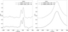 |
Fig. 1 Examples of HR10 (left) and HR21 (right) Gaia-ESO CCFs for the star CNAME 23354061-4305405. Two consecutive observations have been made with each setup. The HR10 epochs t1 < t2 and the HR21 epochs t3 < t4 are separated by less than one day. The S/N of each spectrum used to compute the Gaia-ESO CCF is indicated as labelled. While the SB2 nature of the system is evident from the HR10 Gaia-ESO CCFs, it is not the case from the HR21 CCFs. CCFs are shifted vertically by 0.5 for the sake of readability. |
3 Methods
3.1 DOE
In Merle et al. (2017), the semi-automated tool Detection of Extrema (DOE) was applied to the fourth internal Gaia-ESO data release (iDR4) in order to identify spectroscopic binaries. The main characteristics of DOE are briefly summarised below; more details can be found in Merle et al. (2017) and in particular, Fig. 7 of Merle et al. (2017) illustrates the result provided by DOE on the simulated spectrum of a binary system. DOE takes as input the cross-correlation function (CCF) of a given spectrum and returns the number and position of the detected CCF peaks, that is to say the number and the radial velocity of the stellar components forming the system.
To this end, DOE computes the first, second and third derivatives of the CCF by convolving it with, respectively, the first, second and third derivative of a narrow Gaussian kernel. This technique avoids the numerical noise that may appear when one does discrete differentiation. From the successive derivatives, DOE searches for local CCF maxima and for inflexion points, in order to disentangle the spectral components. The CCF is then fitted by a multi-Gaussian model around the local maxima and/or inflexion points in order to obtain the velocity of the identified spectral components. In Merle et al. (2017), we explained how we have adjusted three user-defined parameters to allow an efficient detection of the CCF components and to automatically obtain results matching those of a visual inspection of the CCFs.
We note that several physical phenomena, distinct from binarity, can produce multiple peaks in a CCF. For example, the Schwarzschild scenario explains double-peak CCFs due to shock wave propagation in Mira star atmospheres (e.g. Alvarez et al. 2000). Cepheids can also display CCFs with multiple peaks (Anderson 2016). However, such stars are rare within the Gaia-ESO Survey.
3.2 Getting narrower HR21 CCFs
When applying DOE to the iDR4 sample in Merle et al. (2017), we realised that the efficiency of the SBn ≥ 2 detection was somewhat setup-dependent as illustrated in Fig. 1. Two pairs of observations of an SB2 are presented, namely two HR10 observations obtained during the same night (left panel) and two HR21 observations obtained the following night (right panel). The four spectra used to compute the CCFs all have S/N > 15. The puzzling fact is that two CCF peaks are clearly visible only in the HR10 observations and not in any of the HR21 observations while the two pairs of spectra are taken within 24 h. Of course, this could be due to a rapid change of the radial velocities or to the slightly lower resolution of the HR21 settings (HR10: R ∼ 21 500 vs. HR21: R ∼ 18 000). However, this alone does not explain the boxy and wide peak with a full-width at halfmaximum (FWHM) of about 100 km s−1 of the HR21 CCFs. Actually, the HR21 setup hosts different spectral features than HR10, some of which have broad wings (e.g. Ca II triplet lines) which can broaden the CCF and hide a double peak. We also suspected the HR21 cross-correlating masks to be less adapted to the HR21 setting. Such investigations have led us to set up a procedure to recompute CCFs by using a set of optimised cross-correlating masks.
Choice of the template stars. We selected a dozen template stars among the Gaia FGK benchmarks (Jofré et al. 2015). These template stars were chosen such that they are representative of the stars observed in HR10 and HR21. Indeed, the stellar parameter space sampled by the HR10 and HR21 targets can be estimated from the recommended stellar parameters provided for iDR5: 90 % of the Gaia-ESO targets with a recommended temperature, surface gravity and metallicity span the ranges [4200, 6700] K, [2.2, 4.7] and [−1.1, 0.3] dex respectively. Table 1 lists our final choice of template stars and their stellar parameters. The stellar parameters of our template stars adequately match the Gaia-ESO parameter ranges given above. The main selection criteria are the effective temperature and the surface gravity, such that our template sample contains six main-sequence stars and six evolved stars with various metallicities: hot (8000 K) and cold (4300 K) dwarfs (log 𝑔 ≈ 4) and hot (5000 K) and cold (4000 K) giants (log 𝑔 ≈ 2).
Cross-correlating masks. One standard way to compute the cross-correlation function for a given observed spectrum is to convolve this observed spectrum with a template spectrum (e.g. a synthetic spectrum or a reference observed spectrum). Usually, one tries to use a template spectrum that matches the target spectrum in order to avoid spurious features in the CCF caused by spectral mismatch and in order to get a very contrasted crosscorrelation function (i.e. its maximum or minimum, depending on how the cross-correlation function is computed, is significantly different from the typical level of the correlation noise). However, in order to obtain narrower HR21 cross-correlation functions, we noticed that a template spectrum built with only carefully selected absorption lines was a better choice, especially to ignore the very wide Ca II triplet lines in the computation. Our criteria to keep a line for a given template star were as follows: a) the line should not be blended; b) the line should not be saturated; c) the normalised flux at the line centre should be higher than ∼0.3. To ease the selection of lines, we designed an automatic tool (Van der Swaelmen, private comm.) to scan atomic lines in a synthetic spectrum and quantify their blendedness and depths. We limited our study to atomic lines of light, α- and iron-peak elements: Na, Mg, Al, Si, Ca, Sc, Ti, V, Cr, Fe, Co. This choice of elements warrants a sufficient number of lines (i.e. > 10) within the spectral range covered by both HR10 and HR21 setups. For a given template star of Table 1, our automated line selection procedure is as follows: a) for a given wavelength range and for a given tested element, we compute two spectral syntheses for the star under consideration: one spectral synthesis Stotal that includes all atomic and molecular transitions and one spectral synthesis Spartial that includes all atomic and molecular transitions except those for the targeted element; b) for each transition of the targeted element, we compute a blending score by comparing Stotal and Spartial around the line under study; c) if the line is not blended or is weakly blended, then we check that the line is not too saturated by computing its equivalent width and we check that the intensity at the line centre is above our depth criterion. Figure 2 compares a standard cross-correlating mask (i.e. a simple spectral synthesis with all its absorption lines, in black) to our fine-tuned cross-correlating mask (in red) when Arcturus is adopted as a benchmark and for both GIRAFFE setups. If, after applying our line selection criteria, it was not possible to keep at least ten lines for a given setup and for a given benchmark star, we discarded this star for the considered setup, explaining the absence of HR10 masks for α Tau, β Ara, µ Leo and 61 Cyg A. The last two columns of Table 1 list the template stars used for HR10 and HR21. In the remainder of the paper, these new masks are called NACRE masks and the resulting CCFs will be called NACRE CCFs. On the other hand, the CCFs provided by the Gaia-ESO consortium will be designated Gaia-ESO CCFs. The library of synthetic spectra used for the selection of atomic lines, and the final cross-correlating masks were computed with the radiative-transfer code turbospectrum (Plez 2012), the grid of MARCS model atmospheres (Gustafsson et al. 2008), the VALD database of atomic transitions (Ryabchikova et al. 2015) and the molecular linelists maintained by B. Plez4.
Masking of spectral features in target spectra. By construction, our HR21 masks do not encompass the near-infrared Ca II triplet at 8498 Å, 8542 Å, and 8662 Å, nor the H lines from the Paschen spectral series, nor the Mg I line at 8806 Å. However, those lines are generally present in the target spectra and may contribute to broaden the HR21 CCF peak and/or create strong correlation noise for large velocity lags (with respect to the target star velocity). A special processing of the HR21 spectra was thus applied in order to mask such strong lines. To this end, we designed an automated procedure to locate the Ca II triplet and the Mg I lines in the HR21 spectrum, fit them with a Lorentzian profile and, if the fit converges and the (normalised) flux at the line centre is below an arbitrary threshold (fixed to 0.8), we subtracted the fit from the observed spectrum, which resulted in an effective masking of these strong Ca II and Mg I lines. Most of the Paschen lines, when they exist, are close to the Ca II lines and we assume they are removed at the same time as the Ca II lines are removed.
Telluric bands are also present at the red end of the HR21 spectral range. Since these telluric bands tend to decrease the contrast of the NACRE CCFs, we decided to mask the last ≈40Å of the HR21 spectra (we replace the fluxes by 1 since we compute the CCF for 1 − f (λ) where f is the observed spectrum or the mask). The red spectrum in Fig. 3 is the result of the described masking procedure applied to one observation of the object with CNAME5 23354061-4305405 while the black spectrum is the original observation. A spectral feature likely to be removed is indicated by a blue line above the spectrum. In the displayed example, the Lorentzian fit of the Mg I line at 8806 Å failed (line not deep enough with respect to our decision criterion) and the spectral chunk is left untouched at these wavelengths. On the other hand, the Ca II triplet is successfully subtracted and, over this range, the modified spectrum is similar to the spectrum in non-modified regions, that is to say the subtraction procedure did not produce any spurious signal. This exposure has a median S /N of 30, which means that weak lines are still present in the spectrum after cancelling out the calcium lines.
Analysis of NACRE CCFs. With the NACRE masks and the cleaned observed spectrum at hand, the next step is to compute all CCFs for a given observation (obtained with a given setup) by using all our NACRE masks (prepared for a given setup). Figure 4 shows all HR10 and HR21 CCFs computed for the star with CNAME 23354061-4305405 and also displays the Gaia-ESO CCF in black.
One sees that despite the relatively small number of lines included in our masks, the HR10 NACRE CCFs overlap with the HR10 Gaia-ESO CCF. On the other hand, as sought for, the HR21 NACRE CCFs have a very different shape from that of the Gaia-ESO CCF: they are always narrower. For the model-case of the target with CNAME 23354061-4305405, the HR10 and HR21 NACRE CCFs now carry the same information concerning the binary nature of the object.
At the end of the computation step, a dozen NACRE CCFs are available for each observation. In order to keep only one NACRE CCF per observation, we rank the series of CCFs by a quantity that estimates their contrast, that is to say the difference between the maximum intensity of the CCF to the typical intensity of the cross-correlation noise measured in the side (or feet) of the CCF peak. The NACRE CCF with the highest grade is called the best NACRE CCF and will serve as a reference during the analysis. The NACRE CCFs whose grade do not meet some conditions (adjusted empirically once and for all) are discarded since they are considered to be dominated by the correlation noise. Such cases become more frequent when the S/N of the spectrum decreases. The reader should note that all the CCFs displayed in this article have been normalised so that the highest CCF component always peaks at 1.
For each observation, DOE is run on the best NACRE CCF as well as on the other grade-selected NACRE CCFs and it returns the radial velocity of each spectral component found in the different CCFs, obtained by fitting the upper part of relevant CCF peaks by a multi-Gaussian function. For each CCF, we use an estimate of the correlation noise (measured in the left and right feet of the CCF peak) to adjust the intensity threshold needed by DOE(one of its user-defined parameter) to disentangle local maxima associated with a possible stellar component from local maxima due to the correlation noise. As for the results obtained for a given observation, different situations may happen, that we classified as follows:
all the masks agree, that is to say DOE finds the same number n of stellar components in the different CCFs and they are at (nearly) identical velocities. The spectrum under study thus hosts n stellar components and their respective velocities are read from the best-mask NACRE CCF (i.e. with the highest rank);
the masks partially disagree, that is to say n stellar components are found in i masks while m stellar components are found in j masks and the n (respectively, m) radial velocities returned by the i (respectively, j) masks agree within the error bars. Then, we read the results from the CCFs characterised by the largest number of components if it also includes our best NACRE CCF (if not, then the observation is flagged for visual check);
the masks strongly disagree, that is to say it is not possible to reduce the results in only two classes of solutions as in the previous situation. Then, we are not able to make an automated decision and the observation is flagged for visual check.
This reasoning holds because, as explained in the first paragraph of this section, our Gaia-ESO star sample spans a relatively small range of effective temperatures (FGK stars), surface gravities and metallicities, and therefore, the spectral mismatch between an observation at one end of the temperature (respectively, gravity, metallicity) range and a NACRE mask at the other end will not change drastically the shape of the NACRE CCF. In other words, when we are not working in the low S/N regime (S/N < 5 – 10), if a stellar component is at a given velocity in one NACRE CCF, it will also appear at a close velocity in another NACRE CCF. The small changes from one mask to the next in measured velocities can be explained by various factors such as the S/N of the spectrum, the set of lines used in the cross-correlating mask, the spectral mismatch, etc. and will be investigated in the next section. Figure 4 illustrates this fact for one HR10 and one HR21 observation. One sees that all our CCFs tend to have a similar shape: for both HR10 and HR21 NACRE CCFs, they exhibit two stellar components, located at similar radial velocities.
Template stars and their stellar parameters (taken from Jofré et al. 2015).
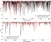 |
Fig. 2 Comparison for HR10 (top) and HR21 (bottom) of our cross-correlating mask (NAC RE mask; red line) to a standard one (black line; e.g. the one that would be used to compute the Gaia-ESO CCFs) computed from a spectral synthesis with Arcturus stellar parameters. Our NACRE mask includes only weak and isolated lines. Despite our strong constraints, more than 20 lines are kept in both HR10 and HR21 masks for Arcturus. |
 |
Fig. 3 Example of spectral feature removal and masking in a HR21 spectrum. The black line stands for the original HR21 spectrum of CNAME 23354061-4305405 (MJD = 56856.376009; median S/N ≈ 30); the red line stands for the modified version of the spectrum, with the Ca II triplet cancelled out and the telluric bands masked while the Mg I line at 8806 Å is left untouched because the criteria were not met (see text). There is a small shift between the vertical marks and the position of the absorption lines since the spectrum is not corrected for the stellar radial velocity (the spectrum is in the heliocentric frame); our algorithm performs a small exploration around the laboratory wavelength to find the observed position of the calcium and magnesium lines to be removed. |
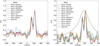 |
Fig. 4 Comparison of Gaia-ESO (dashed black line) CCFs and NAC RE (other solid coloured lines) CCFs for a given HR10 (left; MJD = 56857.311765) and the corresponding HR21 (right; MJD = 56856.376009) observation of CNAME 23354061-4305405. The mask names are provided in the legend boxes. For each observation, all NACRE CCFs agree very well: they have the same shape, they exhibit the same number of stellar components at nearly identical radial velocities. While the HR21 Gaia-ESO CCF exhibits only one stellar component, our CCFs reveal the presence of two stars, in agreement with the HR10 observation. The CCFs are all normalised by their respective maximum for the sake of readability. |
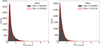 |
Fig. 5 Distribution of σ[υrad,Nacre] with (red line) or without (filled black area) a cut on the S/N (binwidth = 0.016 km s−1). Left: HR10 setup; 〈σ[υrad,Nacre]〉 = 0.39 km s−1 with S/N ≥ 3. Right: HR21 setup; 〈σ[υrad,Nacre]〉 = 0.40 km s−1 with S/N ≥ 3. With or without the S/N cut, most of our sample is characterised by a standard deviation on the radial velocities measured from the different NACRE CCFs below 1 km s−1; the S/N cut depopulates the right tail of the HR10 distribution. |
3.3 Quality control
The nice agreement between the radial velocities provided by all NACRE CCFs is illustrated in Fig. 5 plotting the distribution of the dispersion σ[υrad,Nacre] of the NACRE radial velocities υrad,Nacre. In this figure, we consider only a) individual observations where DOE detects a single stellar component in the NACRE CCFs and b) spectra for which the S /N reported by the Gaia-ESO exists and is either > 0 (in black) or > 3 (in red). We note that this is an ‘observation-wise’ distribution, that is to say it is based on individual observations and a given star may count more than once. While both distributions peak at 0.2 km s−1 for HR10 observations, the black distribution exhibits a more extended tail than the red distribution. The fact that this extended tail disappears at higher S /N clearly shows that the S /N is the main responsible of the velocity dispersion from one mask to the other. The red distribution shows that a S/N as low as 3 is acceptable for our purposes since, in that case, most of the distribution is still below 1 km s−1 and the largest dispersion is around 3 km s−1. On the other hand, for HR21, the cut on the S /N has no effect on the shape distribution. This can be understood because a) HR21 spectra have on average a higher S/N than HR10 spectra and b) the HR10 spectral range for FGK stars tends to contain more weak metallic lines than the HR21 spectral range. Therefore, at low S/N (< 3), in HR10 spectra, the scatter in the flux due to the photon noise has a higher probability (compared to the HR21 case) to mimic a spectral feature that will cause a slight shift in the position of the CCF peak. Like for HR10, the HR21 red distribution peaks at 0.2 km s−1 and most of the distribution is below 1 km s−1. We conclude that the velocities returned by the different masks for a specific observation are most of the time equivalent.
Figure 6 shows the distribution (observation-wise) of the difference υrad,Nacre,j − 〈υrad, Nacre〉masks, where υrad, Nacre,j is either the velocity υrad, Nacre, best derived from the best-mask NACRE CCF (red histogram), or a velocity υrad,Nacre,rand randomly picked up among the series of CCF velocities (black histogram). 〈υrad,Nacre〉masks is the mean velocity over all of the selected NACRE CCFs. The black distribution is centred around 0 km s−1 while the red distribution exhibits a small offset (0.2km s−1) for HR10 and shows no offset for HR21. However, the red distribution is narrower (standard deviations: 0.59 km s−1 for HR10; 0.41 km s−1 for HR21) than the black one (standard deviations: 0.69 km s−1 for HR10; 1.5 km s−1 for HR21), indicating that our ranking criterion for the CCFs is more efficient than a random selection among the measured velocities.
In order to check the reliability of the NACRE radial velocities, we also compared them to the Gaia-ESO recommended radial velocities υrad,GES. Figure 7 displays the distribution (observation-wise) of the differences υrad,Nacre,best − υrad,GES. The mean difference between υrad,Nacre,best and υrad,GES is −0.27 km s−1 for HR10, while it amounts to 0.07 km s−1 for HR21. These numbers demonstrate that the agreement of our velocity scale to the two Gaia-ESO velocity scales is rather good: only HR10 NACRE radial velocities are affected by a small offset that is not corrected for in the Table B.1.
Figure 8 shows the density map of σ[υrad,Nacre] as a function of Teff,GES (recommended Gaia-ESO effective temperature) and [Fe/H]GES (recommended Gaia -ESO Fe abundance). We note that σ[υrad,Nacre] increases towards the cold effective temperature for both HR10 and HR21; the trend σ[υrad,Nacre] vs. Teff,GES tend to be flat for temperatures hotter than 5000 K but the scatter around this flat trend becomes larger above 5500 K. σ[υrad,Nacre] increases for [Fe/H]GES ≤ −1 for both setups, and for HR10 only, σ[υrad,Nacre] increases for [Fe/H]GES ≥ 0. The cross-correlation requires the presence of spectral features to work: the precision of this technique thus decreases for metal-poor and/or hot objects.
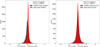 |
Fig. 6 Distribution of ∆= υrad,Nacre,ref− 〈υrad,Nacre〉masks (binwidth = 0.02 km s−1) where υrad,Nacre,jis either the velocity υrad,Nacre,best returned by the bestmask NACRE CCF (see text; red) or a randomly chosen NACRE velocity υrad,Nacre,rand (black). Left: HR10 setup. Right: HR21. The mean, standard deviation and interquartile range of each distribution, expressed in km s−1, are: (0.17,0.59,0.22) for HR10 and ‘best mask’; (0.01,0.77,0.39) for HR10 and ‘random mask’; (0.02,0.38,0.33) for HR21 and best mask; (0., 0.50,0.41) for HR21 and random mask. The number of objects in a given selection is indicated in the legend box. The distributions are narrower for υrad,Nacre,best than for υrad,Nacre,rand. |
3.4 Error budget
Once a local maximum of the CCF is associated with a stellar component, DOE performs a local fit of the CCF (with the help of the Python numpy’s function numpy.optimize.curve_fit) by a Gaussian (or by a multi-Gaussian function in case of multiple stellar components) in order to retrieve the position of this maximum, that is to say the radial velocity of the stellar component. The fitting function returns the parameters defining the Gaussian as well as the associated covariance matrix. The diagonal element of the covariance matrix corresponding to the velocity rvv directly provides the 1σ uncertainty  on the radial velocity due to the fitting procedure. A typical value of this source of uncertainty is 0.01 km s−1.
Figure 9 illustrates the dispersion σ[υrad,Nacre] as a function of Teff,GES − Tmask,best where Teff,GES is the effective temperature of the star and Tmask,best is the effective temperature of the mask of the best-mask NACRE CCF. Since we plot single observations, a given star may contribute more than once to this map. The star’s temperature is the recommended effective temperature provided by the Gaia-ESO working group dedicated to the final homogenisation (WG15) at the end of the iDR5 analysis round. Therefore, in Fig. 9, only the targets with a recommended temperature are displayed. The quantity Teff,GES − Tmask,best can be interpreted as a measure of the spectral mismatch between the analysed star and the best template spectrum. The mask called ‘alphaCenA’ (Teff ≈ 5800 K) yields the best-mask NACRE CCF for the vast majority of the HR10 observations, while the mask called ’betaAra’ (Teff ≈ 4200 K) yields the best-mask NACRE CCF for the vast majority of the HR21 observations. This explains why the quantity Teff,GES − Tmask,best tends to be negative for HR10 and positive for HR21.
We also note that the diagram does not exhibit any clear relation between σ[υrad,Nacre] and Teff,GES − Tmask,best: the distribution is rather flat, with a high density of points around the line σ[υrad,Nacre] ≈ 0.15 km s−1 while an extended poorly populated tail exists at any Teff − Tmask,best. Thus, one can conclude that the uncertainty due to the spectral mismatch on a single radial velocity measurement typically amounts at least to 0.15 km s−1. Some vertical stripes are visible: they are likely due to the sampling of the temperature grids used by the Gaia-ESO analysis nodes.
Figure 10 shows the density map of ∆ = υrad,Nacre,best − υrad,GES and σ[υrad,Nacre] as a function of S/N where υrad,GES is the recommended Gaia-ESO radial velocity. There is no trend between ∆ and S/N but the scatter increases with decreasing S/N: a low S/N does not introduce significant biases in υrad,Nacre,best but degrades its precision. The latter is also shown by the decreasing trend of σ[υrad,Nacre] with S/N, displayed in the bottom panel of Fig. 10. We also notice that the radial velocity precision increases faster with the S/N for HR10 than for HR21 due to the fact that there are more weak lines in HR10 than in HR21.
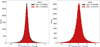 |
Fig. 7 Distribution of ∆ = υrad,Nacre,best − υrad,GES for HR10 (left) and HR21 (right) observations where υrad,GES is the recommended Gaia-ESO RV. We show in black the case S/N ≥ 0 and in red, the case S/N ≥ 3. The mean, standard deviation and interquartile range of each distribution, expressed in km s−1, are: (−0.24, 1.47, 0.67) for HR10 with S/N > 0; (−0.25, 1.23, 0.56) for HR10 with S/N > 3; (0.07, 3.77, 1.05) for HR21 with S/N > 0; (0.07,3.77,1.03) for HR21 with S/N > 3. The number of objects in a given selection is indicated in the legend box. For HR21 (right), the two histograms are almost identical and the black one is not visible. |
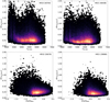 |
Fig. 8 Density map of σ[υrad,Nacre] as a function of Teff,GES (top) and [Fe/H]GES (bottom) for HR10 (left) and HR21 (right) observations. The temperature Teff,GES and the metallicity [Fe/H]GES are respectively the Gaia-ESO recommended temperature and Fe abundance. The number of objects in a given selection is indicated in the legend box. White areas denote zones of the plane where there is no data. |
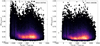 |
Fig. 9 Density map of σ[υrad,Nacre] as a function of Teff,GES − Tmask,best for HR10 (left) and HR21 (right) observations where Teff,GES is the recommended Gaia-ESO effective temperature and Tmask,best is the temperature associated with the best-mask NACRE CCF. The number of objects in a given selection is indicated in the legend box. White areas denote zones of the plane where there is no data. |
4 Results
4.1 Double-lined spectroscopic binaries
Our analysis of the iDR5 sub-sample (as defined in Sect. 2.2) with the help of the NACRE CCFs and DOE, has led to the discovery of 322 SB2 (four of them being also classified as tentative SB3) among the 37565 Milky Way field stars forming the parent sample. The cross-match of the SB2 sample with Gaia DR3 is provided in Table A.1 and the radial-velocity time-series, together with CCF-related quantities, are provided in Table B.1.
Figure 11 illustrates the distribution (per observation; that is to say a given object may count more than once) of the S/N of the spectra used to compute the CCFs in the case of SB2 detections. The S/N of the target spectrum can be as low as 3 – 4 for HR10 and 5 – 6 for HR21 and it still allows the detection of multiple stellar components in the CCF. The HR10 and the HR21 distributions have a different shape: the HR10 (resp., HR21) distribution peaks at S/N ~ 15 (resp., S/N ~ 25); the mean S/N is 15 for HR10 and 32 for HR21. The differences in the S/N distribution of the SB2 detections for both setups are mainly due to the different properties of their parent distribution, that is to say the S/N distribution of their parent HR10 and HR21 samples, respectively. We have indeed a mean S/N ~ 10 for all of the investigated HR10 spectra and a mean S/N ~ 22 for all of the investigated HR21 spectra.
We note also that 65% (resp., 86%) of the investigated HR10 spectra have an S/N lower than 10 (resp., 20), while it is the case for only 29% (resp., 57%) of the investigated HR21 spectra. Logically, we have more detections at S/N lower than 20 for HR10 (297 out of 390, i.e. 76%) than for HR21 (133 out of 473, i.e. 28%). Similarly, in the S/N range [0, 20], we have 297 SB2 detections among 69 475 HR10 observations (0.43%), while we have 133 SB2 detections among 46 047 HR21 observations (0.29%). These statistics show that we probably miss more SB2 detections at low S/N with HR21 than we do with HR10 because of a low S/N. This could be due to the fact that the HR10 wavelength range hosts more (weak) metallic lines for FGK stars than the HR21 wavelength range does, such that even at low S/N, all those absorption lines build up a meaningful HR10 CCF.
The ratio of the number of HR10 SB2 detections (observation-wise) to the number of analysed HR10 observations (390/80 490, i.e. 4.8%) is lower than the ratio of the number of HR21 SB2 detections to the number of analysed HR21 observations (473/80 237, i.e. 5.8%). We already commented on the fact that low values of S/N probably decrease the SB2 detection efficiency in HR21 observations compared to HR10 observations. For S/N larger than 20 (referred to as ‘high S/N’ in the next sentences), we do not see significant differences in the detection efficiency between HR10 and HR21: we have 93 SB2 detections among 10 323 HR10 observations (0.91%), while we have 340 SB2 detections among 34 053 HR21 observations (1.0%). This suggests that the excess of HR21 spectra at high S/N compared to HR10 explains why we have more SB2 detections among HR21 observations than among HR10 observations. In other words, the overall lower quality of HR10 spectra (compared to that of HR21 spectra) hampers the detection of SB2 and may cost up to about 100 HR10 SB2 detections (assuming we can apply the detection rate measured above for the HR21 observations to the HR10 case).
Figure 12 displays the distribution (per observation) of the radial velocity differences (i.e. difference between the two components of the binary system) for both setups. The two distributions are very similar. In each case, the smallest detectable ∆vrad is about ~25 km s−1, they peak at ∆υrad ~ 25 – 30 km s−1 and they decrease at the same rate towards higher ∆υrad. The difference between the HR10 and the HR21 resolutions does not translate into a difference between the smallest detectable ∆υrad for each setup (see also Sect. 4.4 ).
In conclusion, thanks to the NACRE CCFs, our analysis is almost not sensitive to setup effects (spectral range, spectral resolution) in terms of smallest detectable ∆υrad, which was the goal of our effort in developing a new detection technique; another demonstration of the improved SBn-detection efficiency is given in the Section 4.4 with a comparison to Merle et al. (2017). Our technique remains sensitive to the S/N of the underlying spectra: though the minimum S/N required for a detection can be as low as 3–4, poorer-quality spectra still mean lower number of SB2 detections. It remains also sensitive to the spectral content: a low number of weak metallic lines hampers the detection of SB2.
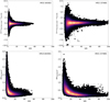 |
Fig. 10 Density map of ∆ = υrad,Nacre,best − υrad,GES (top) and σ[υrad,Nacre] (bottom) as a function of S/N for HR10 (left) and HR21 (right) observations. The number of objects in a given selection is indicated in the legend box. White areas denote zones of the plane where there is no data. |
4.2 Triple-lined and quadruple-lined spectroscopic binaries
We find 12 SB3, of which two may be SB4, among the 37 565 Milky Way field stars. Seven stars were identified both in HR10 and HR21 as probable SB3 candidates, as illustrated in Figure 13. Three tentative SB3 are also listed; they constitute tentative detections since the three peaks are only detected in only one of the two setups. In addition, we provide a tentative detection of two SB4 candidates. The data are summarised in Table 2. They are all faint objects; this is probably the reason why none of them is identified as non-single star by Gaia DR3 (Gaia Collaboration 2023b). Besides, we note that the Gaia mean RVs are not provided, except for the brightest target (CNAME 19243943+0048136, G ~ 14.8). The present spectroscopic-binary study still brings a very new piece of science in the Gaia era since the overlap with Gaia DR3 in terms of advanced Gaia products (e.g. radial velocities, multiplicity or atmospheric parameters) is very small.
Some stars actually display multiple-peaked CCFs without being spectroscopic binaries; this is for example the case of Cepheids (Anderson 2016). However, among the SB3 and SB4 discovered in the present study, only one (CNAME 084020790025437) shows signs of photometric variability (with the Gaia flag phot_variable_flag being raised). Most of the SB3 and SB4 of Table 2 can thus be considered as genuine multiple stars whose number of stellar components (3, 4 or more) will have to be confirmed by future follow-up.
Three SB3 candidates, namely CNAME 08202324- 1402560, 18170244-4227076 and 15420717-4407146, were already detected as spectroscopic binaries by Merle et al. (2017) but only from HR10 observations: the first two already as SB3, while the third one as SB2. With the new masks, they are confirmed as SB3 also with HR21 observations. The three other SB3 are new candidates which were never detected previously and are unknown on Simbad. Among the three tentative SB3, two of them, namely 00195847-5423227 and 15161563-412551, were detected as SB2 in the previous release by Merle et al. (2017). The third one shows proper motion anomaly (Kervella et al. 2019), strengthening the multiple nature of this target.
Additionally, two targets could be SB4 candidates, namely CNAME 18263326-3146508 and 19243943+0048136. Their triple nature is indubitable, and a fourth weak component is observed in their CCFs; they would deserve additional monitoring at higher resolution to confirm their quadruple nature. 18263326-3146508 is not referenced on Simbad but has a very large Gaia RUWE (Renormalised Unit Weight Error). 19243943+0048136 is in the CoRoT field and was already detected as spectroscopic binary (Merle et al. 2017, 2020). We stress that the reliable detection of up to four stellar components in GIRAFFE observations is another direct demonstration of the improved detection efficiency endowed by the NACRE masks: this is a new result compared to our previous study (Merle et al. 2017).
Only three targets among twelve show large Gaia RUWE. This shows that even if a large value of the RUWE points towards the possible multiple nature of sources, it does not catch all of them, especially the distant ones for which the astrometric signal is not detectable, as already well shown in Jorissen (2019) and Kounkel et al. (2021). These three large-RUWE targets can be deemed as a likely SB3, a tentative SB3 and a tentative SB4; they decidedly deserve a spectroscopic follow-up since spectroscopy+astrometry would allow precise masses to be derived.
Finally, we stress that the derived atmospheric parameters (either by Gaia-ESO or by Gaia) are highly unreliable for such composite spectra unless the components have very similar atmospheric parameters and the same radial velocities. Gaia provided such atmospheric parameters for nine targets of Table 2 but they are unreliable for such spectroscopic binaries.
Appendices D6 and E provides the reader with an atlas of CCFs and spectra (classified by increasing MJD for a given system) for all of the detected SB3 and SB4. All available epochs, independently of the number of detected components, are shown; the only requirement is that the computed CCFs are interpretable. This means that according to the stellar waltz occurring between the system’s stars, the reader will see one, two or three (or four for the tentative SB4) stellar components in the CCFs. We emphasise the fact that some of the shown CCFs for the detected SB3 and SB4 are more difficult to interpret than the CCFs of SB2 because the height of the peaks associated with some of the N − 1 stellar components may be comparable to the typical size of the noise. All these systems have been flagged by our pipeline as unusual and have been manually inspected before being classified as SB3 or SB4. As an example, we provide a detailed discussion of the CCFs available for the CNAME 08393088-0033389 (Sect. D.3) and 08402079- 0025437 (Sect. D.4) highlighting the arguments leading to their identification as SB3.
Cross-match of the Gaia -ESO SB3 and SB4 samples, and Gaia DR3.
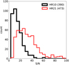 |
Fig. 11 S/N distributions for HR10 (thick black line) and HR21 (thin red line) observations triggering an SB2 detection (binwidth = 5). The histogram is observation-wise, so a given star may appear more than once (in the same or another S/N bin) depending on the observations where the binary nature was detected in. The number of objects in a given selection is indicated in the legend box. |
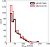 |
Fig. 12 Same as Fig. 11 but for ∆υrad in km s−1 (binwidth = 10 km s−1). The number of objects in a given selection is indicated in the legend box. |
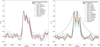 |
Fig. 13 Examples of CCFs for an SB3 (CNAME 18170244-4227076). Left: HR10. Right: HR21. In the HR21 setup, we see how the new masks nicely allow the detection of the three components (coloured CCFs), totally hidden in the Gaia-ESO CCF (dashed black line). The three components were already detected in HR10 with the Gaia-ESO CCF. |
4.3 Locus in the colour-magnitude diagram and comparison to Gaia
We cross-match the Gaia-ESO parent sample (i.e. 37 565 objects) and the Gaia DR3 catalogue (Gaia Collaboration 2023a; Babusiaux et al. 2023): Table 3 gives the count of objects with a published Gaia value for different physical quantities of interest for this study. We use the photometric bands of Gaia DR3 (Riello et al. 2021) to place our SB2, SB3 and SB4 in the colourmagnitude diagram (CMD) displayed in Fig. 14 where ℳG is the absolute magnitude in the G band computed using the apparent G magnitude and the parallax, and GBP − GRP is the colour index. We also use the estimated line-of-sight extinction and reddening given by the fields ag_gspphot and ebpminrp_gspphot in the Gaia source catalogue (Andrae et al. 2023) to construct the extinction-free photometric quantities, denoted by the index 0. Moreover, to plot the CMDs, we apply the following quality filters to clean the parent sample: parallax_over_error ≥ 5 and RUWE ≤ 1.4; after filtering, we are left with 21 880 (resp., 20 730) objects for the reddened (resp., dereddened) CMD. On the other hand, as for the spectroscopic multiples we have detected, we do not apply any filters on their Gaia quantities: if ℳG and GBP − GRP (or their dereddened version) exist, then we show the object in the CMD (SB2 as a red disc, SB3 as a cyan diamond, and SB4 as a magenta plus sign). In the extinction-free CMD, we miss 20 SB2, three SB3 and one SB4 because of missing AG and E(BP − RP) = ABP − ARP. Figure 14 shows both the reddened (left) and dereddened (right) CMD.
Before discussing the CMDs, a word of caution is needed. We remind here that the line-of-sight extinction is estimated by the General Stellar Parameterizer from Photometry (GSP- Phot), part of the astrophysical parameters inference system (Apsis; Bailer-Jones et al. 2013). As explained in Andrae et al. (2023), the Bayesian estimation of AG, ABP and ARP depends on the choice of synthetic spectral energy distributions (SEDs) integrated over the G (resp., BP, RP) passband during the forward-modelling of the magnitude in the G (resp., BP, RP) band. GSP-Phot explicitly targets non-variable single stars and as such, the used synthetic SEDs are computed for single stars only. Therefore, the inaccuracy and imprecision of AG, ABP and ARP might be larger for the objects of our SBn samples than for the other objects of the parent-sample. Another Apsis module, namely Multiple Star Classifier (MSC; Creevey et al. 2023), tries to estimate AG (among other parameters) by assuming that any Gaia source is an unresolved co-eval binary system with a given flux ratio. We note that nearly all of the SBn candidates reported in this article have a Gaia MSC AG. Unfortunately, MSC does not provide an estimate of the reddening and, even if it was available, using both GSP-Phot and MSC estimates to correct the photometry of an object depending on its suspected degree of multiplicity may also introduce other uncontrolled biases in the dereddened CMD. Because of the above issue, in the next paragraphs, we discuss the photometric properties of the SBn with respect to their counterpart in the single-star main-sequence using both the reddened and dereddened CMD.
We note that the SB2s detected in the present paper are mainly distributed along a sequence, shifted upwards (so towards brighter magnitudes) in the uncorrected and in the extinction- corrected CMD, parallel to the main-sequence outlined by the parent sample in black. In order to estimate the mean shift between the SB2 main-sequence and the parent-sample main- sequence, we perform respectively a quadratic and quartic fit of these two sequences over the colour range [0.7, 3.1]. To this end, we rebin in both colour and magnitude the two sequences before fitting the polynomial. A Monte-Carlo simulation (Ndraw= 801) is used to propagate the uncertainties on the Gaia parallaxes, G fluxes, and BP and RP fluxes (uncertainties on the extinction and reddening are not propagated, though) in order to estimate the uncertainty on the locus of the centroid of each sequence. It is illustrated by the green and blue thick lines in Fig. 14. On the dereddened CMD, the mean difference in extinction-free absolute magnitude between each sequence, over the colour range [0.7, 3.1] is 0.78 ± 0.04 mag. This should be compared to the difference of 0.75 mag expected between the absolute magnitude of an SB2 formed of two twin stars and the magnitude of each star taken separately. We note the existence of a small group of SB2 objects fainter than expected: they are below the blue trend and we even see a dozen of them around GBP − GRP ≈ 1 (and similarly, around (GBP − GRP)0 ≈ 1). In the reddened CMD, the two SB2 at coordinates (0.969, 7.94) and (0.983, 7.21) are respectively 14001598-4223091 and 18492379-4232588.
In the extinction-free CMD of Fig. 14, we note that six out of seven SB3 are on the bright side of the SB2 sequence (i.e. above the mean trend). These six objects tend to be 1.03 mag (std. dev. = 0.35 mag) brighter than their counterpart in the parentsample; for a system made of three identical stars, we expect an absolute magnitude brighter by 1.20 mag compared to the magnitude of the star alone. In the reddened CMD, two SB3, namely CNAME 15120307-4049481 (coordinates (1.15, 8.5) in the CMD) and 00195847-5423227 (coordinates (0.92, 5.45)), are surprisingly faint; Gaia DR3 provides extinction estimates for only 00195847-5423227 and this object is still fainter than the other SB3 in the dereddened CMD.
In the reddened CMD, the two tentative SB4 are brighter than the SB2 and SB3 lying in the same colour range. After dereddening, only one SB4 remains − 19243943+0048136 – in the extinction-free CMD: it is moved to the hot-edge of the main- sequence at the coordinates (0.57,2.80). This area of the CMD is less populated by the parent sample and it is outside the range where we parameterised the parent-sample main-sequence. If we compare the magnitude of 19243943+0048136 to the magnitudes of all objects found in a narrow colour-interval of 0.01 mag, centred on the colour of this SB4, then we find a mean difference of 0.52 mag with a standard deviation of 1.09 mag (computed with 61 objects). We remind that the difference in absolute magnitude is 1.51 mag for a system made of four identical stars, compared to the absolute magnitude of each star separately. We note that the computed mean difference is much smaller than the theoretical one but given the weakly constrained mean difference, this test might not be very conclusive.
In the previous paragraphs, we noted that some of the detected SB2, SB3 and SB4 have a suspicious position in the reddened and dereddened CMD. These objects tend to have also a RUWE larger than 1.4. The SB2 forming the small group around GBP − GRP ≈ 1 tend to have a large RUWE (e.g. 01194949-6003364 with a RUWE of 3.979, 00195847-5423227 with a RUWE of 15.259, 15230178-4204383 with a RUWE of 10.961). It is also true for some other SB2 below the blue trend like 02003583-0053539 at reddened coordinates (1.404, 6.49) and with a RUWE of 3.982. And in particular, the two SB2 14001598-4223091 and 18492379-4232588 (outliers in the reddened CMD; not shown in the dereddened CMD) have a RUWE of respectively 3.908 and 11.559. The two SB3 001958475423227 (outlier in both CMD) and 15120307-4049481 (only shown in the reddened CMD) have a RUWE of respectively 15.259 and 11.683. One of the two SB4, 18263326-3146508, has a RUWE of 10.934, while the other, 19243943+0048136 (the only one shown in both version of the CMD), has a small RUWE (0.834). The large values of RUWE indicate a likely unreliable astrometry: thus the parallax could be inaccurate and the object could be further away and intrinsically brighter than computed. Therefore, inaccurate Gaia astrometry due to the non-single nature of the sources could be one of the reason why a fraction of our spectroscopic binaries are significantly fainter than other spectroscopic binaries at similar GBP − GRP.
We note that 5 % of the SB2 have a Gaia radial velocity (Katz et al. 2023), while 3 % of the stars in the parent-sample have one. Given the larger uncertainty on the former value, we conclude that the two samples are equally missing a Gaia estimate for the radial velocity and that the faintness of the source - rather than its degree of multiplicity – is the main explanation for the absence of a Gaia radial velocity. Among the iDR5 sample under investigation, Gaia DR3 flags 27 stars out of the 37 260 as non-single star (field non_single_star of the Gaia main catalogue; Gaia Collaboration 2023b): four are reported as eclipsing binaries (EB) and 23 as astrometric binaries (AB). None of them are identified as SB in the present study: the Gaia EB might be too faint to have Gaia radial velocities, while the Gaia AB could be wide long-period binaries that cannot be caught by a spectroscopic survey not designed for radial velocity monitoring as it is the case for the Gaia -ESO. In addition, we also cross-matched the 803 Gaia -ESO SB1 candidates from Merle et al. (2020) with Gaia DR3 and only nine are flagged as non-single star by Gaia DR3: three as AB, five as SB, and one as EB. The reason of the small number of objects in our SB1 (from Merle et al. 2020) and SBn ≥ 2 (this work) samples flagged by Gaia as SB is that the Gaia SB detection is limited to targets brighter than G ~ 13, while the median V magnitude of Gaia-ESO targets is around 15. Despite the wealth of data brought to the community by the Gaia mission, ground-based spectroscopic surveys still bring newness in the field of SB detection and characterisation.
Other indicators of stellar multiplicity can be found in the Gaia Astrophysical parameters tables: classprob_dsc_ comb- mod_binarystar and classprob_dsc_specmod_binarystar that are the probabilities from the Discrete Source Classifier (DSC; Delchambre et al. 2023) of being a binary star, probability obtained using either the combined spectro-photo-astrometric information (classifier ‘combmod’) or the (BP/RP) spectro- metric information alone (classifier ‘specmod’); flags_msc that is a flag indicating (when set to 1) an unreliable inference result from MSC. Delchambre et al. (2023) shows that the completeness and purity for the class “binary” is poor with the two classifiers: only 0.2% of the unresolved binaries of their validation data-set are recovered (see their Table 3). Given this performance index, we do not expect more than a couple SB2 to be correctly flagged by DSC. Only one SBn (an SB2) has classprob_dsc_combmod_binarystar larger than 0.01. About 80 SB2 (resp., eleven SB2) have classprob_dsc_specmod_binarystar larger than 0.01 (resp., 0.10) and no SB2 has this probability larger than 0.3. Three SB3 have a probability of at least 1 % to be binary according to classprob_dsc_specmod_binarystar, while this field gives a null probability of binarity for the two detected SB4. Using the census from Merle et al. (2020), we find three SB1 out of 803 with a probability classprob_dsc_combmod_binarystar between 1 and 10 %. We conclude that it is not possible to use the fields classprob_dsc_combmod_binarystar and classprob_dsc_specmod_binarystar for a robust selection of binary stars, at least in the Gaia-ESO magnitude regime. Eleven SBn have no MSC parameters; four are flagged as unreliable by MSC; 319 have flags_msc set to the default value of 0.
If we look at the Gaia column ipd_frac_multi_peak (IFMP) giving the percentage of windows with a successful image parameters determination (IPD) and for which the IPD has identified a double peak, then we find: 59 SB2 with a non-null IFMP, only 12 SB2 have an IFMP larger than 10% and the largest IFMP value is 71% for 14001598-4223091; 3 SB3, 00195847-5423227 (IFMP = 30%), 15120307-4049481 (IFMP = 16 %) and 21393685-4659598 (IFMP = 2 %), have a non-null IFMP; one SB4, 18263326-3146508, has a nonnull IFMP (IFMP = 60 %). If we look at the Gaia column ipd_gof_harmonic_amplitude (IGHA) whose a large value indicates that the source has some non-isotropic spatial structure, then we find 162 SB2 (resp., 63), two SB3 (resp., two) and two SB4 (resp., two) with an IGHA larger than 0.022 (resp., 0.051), where 0.022 (resp., 0.051) is the median IGHA of the parent sample (resp., the median IGHA increased by its interquartile range). We conclude that a future release of Gaia should be able to correctly flag at least some of the SBn uncovered in this work as binaries.
Figure 15 shows the cumulative distributions of Gaia-ESO SB2 discussed in this study, of all SB from the SB9 catalogue and of Gaia ABs and SBs7 (Gaia Collaboration 2023b) as a function of their Gaia distance. We see that nearly 100 % of the Gaia DR3 AB are detected within 2 kpc from the Sun while 30 % of the Gaia SB (i.e. ~65 000 systems) are at a distance larger than 2 kpc and up to 8 kpc. We note that the Gaia-ESO SB2 also sample large distances: 40 % of them are at a distance larger than 2 kpc; for distances larger than 3.5 kpc, the cumulative distribution of Gaia-ESO SB2 and Gaia SB overlap.
To summarise this section, the extinction-free Gaia CMD shows that the SB2, SB3 and SB4 we detected in the iDR5 parent-sample tend to be brighter than the average magnitude of stars from the parent-sample in the same colour range: this photometric argument strengthens the spectroscopic detection. In particular, the sequence outlined by the SB2 lies 0.78 mag above the sequence of the bulk sample. The cross-match with Gaia DR3 establishes that none of the SB2, SB3 and SB4 listed in this work are flagged as non-single star by the Gaia main source catalogue. Thus, future ground-based spectroscopic surveys, like WEAVE or 4MOST, whose resolution is similar to the Gaia-ESO GIRAFFE observations, will play an essential role in the profiling of the Milky Way spectroscopic binary population.
Count of objects with a published given Gaia physical quantity or fulfilling a given condition.
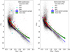 |
Fig. 14 Colour-magnitude diagram of the Gaia-ESO parent sample (black dot). Spectroscopic binaries are overplotted: SB2 (red disc), SB3 (cyan diamond), and SB4 (magenta plus). ℳG is the absolute magnitude in the G band. The blue and green thick lines are respectively a quartic and quadratic fit of the rebinned parent-sample main-sequence and of the rebinned SB2 sequence. The width of the lines materialises the 1 – σ uncertainty on the locus of these two trends only due to the uncertainties on the parallaxes and photometry; the thickness of these lines is therefore not related to the vertical scatter of the datapoints. Left: photometric quantities are not corrected for the extinction. Right: photometric quantities are corrected for the extinction by using AG and E(GBP − GRP) from Gaia DR3. |
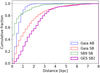 |
Fig. 15 Comparison of the cumulative distributions of Gaia -ESO SB2 (magenta; this work), Gaia astrometric binaries (blue) and spectroscopic binaries (red; Gaia Collaboration 2023b), and spectroscopic binaries from the SB9 catalogue (green; Pourbaix et al. 2004) as a function of the distance from us. The SB9 catalogue was cross-matched using the CDS X-match service (Pineau et al. 2020) with Gaia DR3 (Gaia Collaboration 2023b). |
4.4 Comparison to Merle et al. (2017)
In this subsection, we compare the results regarding our SB2 detection to the results in Merle et al. (2017). Merle et al. (2017) ran DOE on the Gaia-ESO CCFs, while in the present study, we run DOE on the NACRE CCFs. The comparison of the SB2 reported here to those reported in Merle et al. (2017) will thus allow us to judge the efficiency’s gain offered by the NACRE CCFs. However, the comparison is not straightforward because a) the present study focuses on the Milky Way field stars observed in HR10 and HR21 while Merle et al. (2017) analysed the whole Gaia-ESO dataset and b) the present study relies on iDR5 data while Merle et al. (2017) used iDR4 data. Hence an observation exhibiting a binary signature in the present work will be considered for the comparison only if it fulfils the following criteria: a) the target was already part of the iDR4 release; b) the target is observed at least once with either HR10 or HR21; c) the target is a Milky Way field star (its field is thus labelled as GES_MW_XX_YY in the Gaia-ESO notation). We note that 116 734 HR10 and HR21 spectra (27 344 objects) with a field GES_MW_XX_YY are found in iDR4; when this study’s iDR5 parent-sample is restricted to the MJDs covered by iDR4, it is downsized from 160 727 spectra (37 565 objects) to 114 850 (27 006 objects). The set of spectra is smaller than that of the fourth data-release since some targets were removed from the Gaia-ESO target list between the two internal releases.
Merle et al. (2017) identified 342 SB2 within the full iDR4, that is to say including also observations obtained with other setups than GIRAFFE HR10 and HR21 and observations of cluster stars. In Merle et al. (2017), 158 SB2 out of the 342 fall within our selection criteria (HR10 or H21, GES_MW_XX_YY); but three objects, namely CNAME 09594300-4054056, 095946504059014 and 10004160-4053496, shall be removed since they are not in the iDR5 target list. As a result, from Merle et al. (2017), we keep 187 HR10 and 152 HR21 observations exhibiting a binary signature, which corresponds to 155 SB2. We will refer to this sample as ‘iDR4 analysis’. And from this study, we keep 278 HR10 and 333 HR21 observations exhibiting a binary signature, which corresponds to 227 SB2. This sub-sample is seen as a re-analysis8 of iDR4 HR10 and HR21 spectra with the NACRE CCFs in lieu of the Gaia-ESO CCFs. That being said, for the sake of clarity, we will now refer to this sample as ‘iDR4 re-analysis’.
Taking the number of SB2 detections in both setups at face value clearly demonstrates that the use of the NACRE CCFs allows us to significantly increase the number of detections when we re-analyse the iDR4 sample. The number of detections (in terms of observations) is increased by 611/339 ≈ 1.8, while the number of detected SB2 is multiplied by 227/155 ≈ 1.5. In particular, it is striking to see that the number of SB2 detections based on HR21 spectra is more than doubled thanks to our new way of computing the cross-correlation functions. We note however that 29 of the 155 iDR4 SB2 are absent from the iDR4 re-analysis. These objects are characterised by observations with low S/N: 43 out of the 117 exposures available for these 29 targets have S/N ≤ 5, 74 have S/N ≤ 10. The good exposures, most of them obtained with HR21, can have S /N as high as 80 but a visual inspection of the spectra points at low metallicity and/or hot (≥ 6000 K) objects. As a consequence, the strongest lines visible in HR21 spectra are the Ca II triplet, that is to say the lines that we discard to avoid excessively broad CCFs. The HR10 and HR21 CCFs of these metal-poor and/or hot objects tend to have large correlation noise, making the interpretation of secondary maxima as stellar component(s) difficult.
Figure 16 shows the distribution (per observation) of the radial-velocity differences between the two components of SB2 CCFs for the iDR4 sample (left) and the re-analysed iDR4 sample (right). For the iDR4 sample, we note that the distribution for HR21 (red) starts at ∆υrad ~ 60 km s−1 while the distribution for HR10 (black) starts at ∆υrad ~ 25 km s−1. This was already noted in Merle et al. (2017): the Gaia-ESO CCFs for HR21 tend to be broader than their HR10 counterpart which hampers the detection of SB2 with small ∆υrad. On the other hand, for the iDR4 re-analysis, we note that the ∆υrad distributions for HR10 and HR21 roughly start at the same value ∆vrad ~ 25 km s−1. This fact also demonstrates the gain offered by the NACRE CCFs: we are now able to sample the same ∆υrad with both GIRAFFE setups. The HR10 ∆υrad distribution of the iDR4 re-analysis resembles the one of the primitive iDR4 analysis, except that the bins are more populated. This is another check that our NACRE masks return reliable velocities and do not introduce new biases in the velocity measurements (e.g. new bias that could have been caused by the limited number of lines in the NACRE masks). The mean and standard deviation of the difference ∆4–5 = υiDR4 – υiDR5 between the velocities of SB2 common to Merle et al. (2017) and the iDR4 re-analysis (this study) are: 0.1 km s−1 and 1.3 km s−1 for the first component and −0.04 km s−1 and 1.8 km s−1 for the second component.
Figure 17 compares the number of detected SB2 in the earliest iDR4 analysis and its re-analysis. Here we look at three subgroups: HR10 SB2 (resp., HR21 SB2) contains SB2 only detected with HR10 (resp., HR21) observations, and HR10+21 SB2 contains SB2 detected with both setups. Once again, the comparison of the histogram for the iDR4 analysis and reanalysis shows that the use of the NACRE CCFs radically improves the outcome of the analysis. While in the iDR4 analysis, the largest (resp., smallest) number of detection occurred in the HR10 SB2 group (resp., HR10+21 SB2 group), it is the opposite for the re-analysis. It means that most of the discovered SB2 in the re-analysis have at least one detection in each setup, which implies that the new list of SB2 is more robust. The striking increase in the number of objects in the HR10+21 SB2 group between the initial iDR4 analysis and its re-analysis is explained by the hatched bars: 41 HR10 SB2 and 15 HR21 SB2 in iDR4 have become HR10+21 SB2 in the re-analysis. It demonstrates that the NACRE CCFs indeed increase the detection efficiency in the HR21 observations. We note that the NACRE CCFs also slightly increase the detection efficiency in HR10 observations.
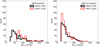 |
Fig. 16 ∆υrad distributions for HR10 (thick black line) and HR21 (thin red line) observations triggering an SB2 detection. Left: earliest iDR4 analysis described in Merle et al. (2017); right: iDR4 re-analysis (this study). We are interested in the individual exposures, therefore an SB2 with more than one epoch will be counted more than once and may appear in different bins depending on the change of its components velocities from one epoch to another. |
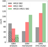 |
Fig. 17 SB2 count depending on the setup(s) triggering the SB2 detection. Black: HR10 SB2, i.e. SB2 detected from HR10 observations only. Red: HR21 SB2, i.e. SB2 detected from HR21 observations. Green: HR10+21 SB2, i.e. SB2 detected from both HR10 and HR21 observations. Left: earliest iDR4 analysis by Merle et al. (2017). Middle: iDR4 re-analysis with NACRE masks. Right: iDR5 analysis (this study). In the left group, the hatched bars overplotted indicate the SB2 objects detected from HR10 only (resp., from H21 only; resp., from HR10 and HR21) in Merle et al. (2017) and that are now detected thanks to both setups in the iDR4 re-analysis. The difference of height between the hatched bar and that of the green bar is explained by about ten iDR4 SB2, formerly detected in both HR10 and HR21, and now detected only with one of the two setups (the best-mask CCF did not exist for S/N reasons in some cases). |
4.5 SB2 detection rate
Using the Ninth Catalogue of Spectroscopic Binaries (SB9) by Pourbaix et al. (2004, 2009), we attempt to estimate the SB detection rate given the quality (mainly, resolution and S /N) of the Gaia-ESO data and the observational strategy followed by Gaia-ESO (i.e. epochs at which Gaia-ESO collected spectra). The SB9 catalogue9 is built from heterogeneous sources: it is a compilation of the orbits of spectroscopic multiple systems published by various authors up to 2021. The latest version (202103-02) contains 1642 SB2 orbits corresponding to 1294 SB2 systems (some systems have several sets of orbital parameters). The SB9 catalogue attempts to provide the spectral types and luminosity classes for each SB2 spectroscopic component. After parsing the columns giving the tentative spectral types and luminosity classes, we find that 788 SB2 have at least one of the two components being a FGK (set 0) star and the remaining SB2 systems have uncharacterised components or both components have a spectral class different than FGK (e.g. O star, white dwarf, Wolf-Rayet star). Among the 788 SB2 of set 0, 326 (324 with full set of orbital parameters) SB2 have a FGK main-sequence star as the primary component (set 1). 108 of 326 systems have a secondary component that is also FGK. Finally, 54 (52 with full set of orbital parameters) SB2 are (quasi-)twin stars (set 2). For some systems, more than one orbit is reported by SB9; in that case, we simply keep the first orbit in the list since our aim is to have a realistic set of SB2 orbits and not the most likely orbit of the system under consideration. In this section, we use both the set 1 and 2 to get two different estimates of the SB2 detection rate within Gaia-ESO iDR5.
Our input Gaia-ESO sample mainly comprises FGK dwarf and giant stars; however, the locus of the Gaia-ESO SB2 in the Gaia CMD shows that the identified SB2 are on the SB2 main sequence. Therefore, for the test described in this section, we decide to use the SB2 listed in the SB9 catalogue for which at least one component is an FGK main-sequence star, i.e. the sets 1 and 2.
To estimate the detection rate of SB2 given the Gaia-ESO observational constraints, we proceed as follows. We list all observed CNAMEs with all their corresponding epochs for the iDR5 parent sample. Thus, one or more epochs (generally, two and four) are attached to a given CNAME. We also associate to each epoch the S/N of the corresponding HR10 or HR21 spectrum. For a given set of N SB9 systems, we randomly associate N CNAMEs (and their corresponding M epochs and M S/N). Then, for each of the N SB9 systems, we use their orbital parameters to compute the velocities of the two components at each of the M Gaia-ESO epochs. For each epoch, we compute the radial velocity ∆υ = υ2 – υ1 difference between the two components. If |∆v| > 30 km s−1 and S/N > 5 and |υ1,2| < 250 km s−1, then we assume a detection. If one of the condition is not valid, we assume that we miss the detection of the two individual components. These criteria correspond to the limitations due to the spectral resolution of the Gaia-ESO spectra or due to our filters to assess the quality of our CCFs for false-positive or very uncertain detections. We emphasise that these simulations only test the SB2 detection from a kinematical aspect (the check is made on the velocity difference) and not from a spectroscopic aspect: we do not generate composite spectra to verify whether the two components are detectable at the same wavelength ranges (i.e. at the HR10 and HR21 wavelengths). This choice is partly constrained by the fact that the stellar components of the SB9 systems are not always fully characterised, preventing us from computing the corresponding synthetic spectrum of a given system. If we restrict ourselves to fully characterised systems formed of two main-sequence stars (not necessarily (quasi-)twin stars), we are left with only 88 systems, which will result in a more imprecise detection rate than what can be achieved with set 1. We repeat the simulations 501 times which is enough to ensure a numerical convergence of our estimated percentages on the unit digit. Since the set of Gaia-ESO CNAMEs is much larger than the set 1 and 2 of SB2 systems, it is equivalent to run the simulations spectral type by spectral type or with all spectral types together. For the sake of simplicity, we perform separated simulations to estimate per-spectral-type rates and we perform simulations on the full sets (1 or 2) for global rates.
Figure 18 shows the distribution of the detection rate for each set (1 and 2) after the 501 simulations. We estimate a mean detection rate of 57.8 ± 2.0% from the set 1 and of 64.8 ± 5.2% from the set 2. If we apply these rates to the number of detected SB2 in our Gaia-ESO sample, we find a number of SB2 between 497 and 557. Given the input Gaia-ESO sample contains about 37 565 targets, we derive an SB2 frequency (among the field stars) in the range [0.0132, 0.0148].
Combining the results from Merle et al. (2020) and from this study, it is possible to compute the spectroscopic-binary-star fraction Fbinary and the spectroscopic-binary frequency fbinary. Merle et al. (2020) found 803 SB1 (their selection with a 3 – σ confidence) among about 43 500 Gaia-ESO targets. Their SB1 is downsized to 581 when restricted to the parent sample used in this study. Applying their detection rate of 25 %, we obtain a theoretical number of 2324 SB1. On the other hand, the theoretical number of SB2 is 528 when we apply an average detection rate of 61 % to the number of detected SB2. This yields a spectroscopic- binary-star fraction, expressed in percentage, of Fbinary≈7.6%. This value is smaller than the binary-star fraction of 30 % quoted by Moe & Di Stefano (2017) for solar-type stars (their Table 13); this can be understood by the fact that their statistics is not restricted to spectroscopically detected binaries, while we are.
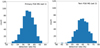 |
Fig. 18 Distribution of the detection rates for set 1 (left; binwidth = 1%) and 2 (right; binwidth = 2%). The y-axis gives the count of simulations with a detection rate within the range defined by the bin coordinates. For instance, for the set 1, ≈94 out of 501 simulations have a detection rate between ≈57% and ≈58%. |
4.6 Mass-ratio distribution
The time series of radial-velocity pairs for the detected SB2s can be used in order to derive the mass ratio q of the system. Indeed, the mass ratio q is given by the absolute value of the slope of the υs vs. υp relation, where υp and υs are respectively the velocity of the primary and the secondary components (e.g. Fernandez et al. 2017). Table B.1 shows that 148 SB2 have at least three epochs, most of them (120) having four epochs. To measure the slope of the υs vs. υp relation, we first need to assign correctly each epoch-velocity at its respective component and then perform a linear regression in the υp – υs plane.
The height of the CCF peak of each component can be a help to follow each component in the CCFs along time. We remind that the selection of the NACRE best mask does not rely on a spectral matching criterion but on a contrast criterion. As a consequence, there is no a priori assurance that the same mask is chosen as best mask for all of the epochs of a given SB2. And indeed, it is empirically confirmed in Table B.1 where we note that alphaCenA is picked as the best mask for the vast majority of HR10 observations, while betaAra is picked as the best mask for all of the HR21 observations. To solve this issue, for a given object and a given epoch, we compute the average Ki of the heights Hi,j of the peak i, measured in the j = 1..Ngood CCFs used for the analysis: the peak with the largest average height gets numbered 1, the other is numbered 2. We repeat this operation for all of the epochs of a given SB2 in order to have a series of velocity υrad,1 (resp., υrad,2) tracking the same stellar component. At this stage, we use the numbering (component 1, component 2) and not the labelling (primary, secondary) since this procedure is not sufficient to pinpoint the primary component (i.e. the most massive in order to have q < 1.). Table B.1 gives the average height of the first-component’ peak K1 = ⟨k1 ⟩CCF, the normalised average heights ki = Ki /K1. By construction, k1 is equal to 1 all the time, except when we manually correct the component assignation (see below). Though we do not make use of those quantities in the present study, Table B.1 gives also the height of the first-component peak H1, the normalised heights hi = Hi /H1, and the widths wi of the components’ peak, all measured in the best-mask CCF. We then inspect the automatic assignations to identify possible errors; this is specified in the column ‘mode’ of Table B.1. For instance, with the automatic ordering, the component 1 of 00410028-3707024 would see its velocity jumping from 21.9 km s−1 to 45.5 km s−1 in about 26 min, hence an acceleration of 54.6 km s−2, at odds with what is observed for the other systems. For 02035132-4215039, we think that the automatic ordering is correct: we have υrad,1 = 43.61 km s−1 and υrad,2 = −21.21 km s−1 at MJD = 56912.325754, and υrad,1 = −4.29 km s−1 and υrad,2 = 36.71 km s−1 at MJD = 56968.141005. We could be tempted to swap the velocities for one of the two epochs but this is hardly justified because the two epochs are 56 days away and k2 is always significantly lower than 1. There are also doubtful cases like 03103980-5007403. For this system, the automatic ordering assigns the velocities υrad,1 = 39.97 km s−1 and υrad,2 = −12.89 km s−1 at MJD = 56310.061037, and υrad,1 = −14.02 km s−1 and υrad,2 = 42.02 km s−1 at MJD = 56312.038016. The two epochs are about two days away, hence an acceleration of −1.14 km s−2 with the automatic assignation. If we were to manually swap the velocities for one of the two epochs, the acceleration would become 0.04 km s−2. Both are plausible accelerations: the former would still be smaller (in absolute value) than the acceleration seen for the component 1 of 07205928-0033063 between MJD = 55998.069876 and MJD = 55998.087887 (k2 is significantly different from 1 to trust the classification); the latter would be similar to what is seen for the component 1 of 05190040-5402093 between MJD = 56312.097403 and MJD = 56314.091117 (same remark on its k2). Besides, for 03103980-5007403, k2 ≈ 0.9, so too close to 1 to help in the decision making.
We now assume that υp = vrad,1 and υs = υrad,2, and perform the linear regression with the help of the scipy routine scipy.odr.ODR, which allows to propagate the uncertainties on both coordinates. We remind here that the radial velocities are adopted from the best-mask CCF. The final statistical uncertainty on the radial velocity is taken as the standard deviation of the velocities measured on all of the masks and corrected for small statistics using the Student’s distribution. We force a minimal uncertainty of 1 km s−1. The absolute value of the slope gives the mass ratio q of the system. If q is larger than unity, then we assume that we made a mistake by considering that the component 1 should play the role of the primary component: we then swap the roles and redo the linear regression. Figure 19 displays the distribution of the mass ratios for 148 systems of the iDR5 SB2 sample; the different colours correspond to different levels of relative uncertainty: the blue histogram displays all 148 systems, while the red histogram displays only the 40 best constrained q (with a relative uncertainty below 10 %). The mean mass-ratio uncertainty e(q) on q is 0.24 and the median uncertainty is 0.19. However, e(q) can be as low as ≈0: this indicates an ill-constrained regression and/or unrealistic errors on the radial velocities. We recommend to use a minimal uncertainty of 0.2 on q for all systems. The blue distribution (all estimates) shows a thick tail for q ⪅ 0.7 and is skewed towards q ≈ 1. The tail for small mass ratios quickly disappear when we impose a more and more stringent quality criterion – a smaller and smaller relative uncertainty – on the estimated q. The red distribution, that should contain the systems with the most robust estimate of q, has most of the q in the range [0.7,1.]: this is expected for SB2 made of FGK main-sequence stars and it is in good agreement with, for instance, Boffin & Pourbaix (2019) and Boffin & Trimble (2020). Indeed, in order to detect the two stellar components in the same spectral range, the two stars should be of similar spectral types and luminosities, and therefore, they should have a similar mass, hence q ≈ 1. Moreover, the red histogram is consistent with the shift in luminosity measured in the Gaia CMD: the uncovered SB2 population is likely dominated by systems with q larger than 0.9, producing a vertical magnitude shift close to 0.75. We therefore advise the end-user to use the published mass-ratios q after applying a filter on the relative uncertainty on q.
5 Summary and conclusion
The main findings of this study are the following:
We crafted a dozen cross-correlating masks, called NACRE, to obtain CCFs as narrow as possible and, as such, to detect RV components with a RV difference as low as possible;
The analysis of 160 727 Gaia-ESO iDR5 GIRAFFE FGK spectra with the NACRE masks and the automated DOE extremum-finding tool led to the detection of 322 SB2 (with four of them also being classified as tentative SB3), ten SB3, and two tentative SB4l
NACRE masks and DOE performances are excellent: the smallest detectable ∆υrad is around 25 km s−1 for both HR10 (optical range, R = 21 500) and HR21 (near-infrared range, R = 18 000), and so ∆υrad is virtually insensitive to the spectral resolution and spectral range of the observations;
The performances are sensitive to the S/N of the spectra: the S/N may however be as low as three or four before preventing any detection.
As any cross-correlation-based technique, our technique relies on the existence of absorption lines in the spectra and is therefore sensitive to the spectral content: NACRE CCFs of metal-poor and hot objects tend to be difficult to interpret. Moreover, at a given S/N and for FGK targets, it is probably easier to detect an SB2 with HR10 than with HR21 since there are more (weak) metallic lines in the HR10 range than in the HR21 range for those stars;
This work shows that excluding pressure-broadened lines such as the Paschen lines or resonant lines such as the Ca II triplet is key for improving the SBn detection rate;
In the extinction-free Gaia CMD, the uncovered SB2, SB3, and SB4 tend to be brighter than their counterpart of the parent sample in the same colour range, advocating the multiple nature of these objects;
Thanks to Monte-Carlo simulations, we estimate the true SB2 frequency to be in the range [0.0132, 0.0148];
We find a mass-ratio distribution for the SB2 skewed towards q = 1, indicating that our SB2 sample is likely mainly made of main-sequence twin-star systems;
None of our SB2, SB3, or SB4 are reported as astrometric, eclipsing, or spectroscopic binaries by Gaia, establishing that ground-based spectroscopic surveys still hold an essential role in the Gaia era to complete the census of binary stars in the Milky Way. In particular, the WEAVE and 4MOST massive spectroscopic surveys will work at a resolution similar to the GIRAFFE HR10 and HR21 resolutions. The present work can therefore find a future application in the context of these soon-to-start surveys.
A future publication will apply the NACRE masks and the approach described here to the final and public release of the Gaia-ESO (namely, DR5, the fifth public data release, corresponding to iDR6, the sixth internal data release). In particular, this work will be extended to Gaia-ESO HR15N observations, which targeted Milky Way stellar clusters.
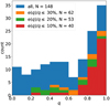 |
Fig. 19 Mass ratio (q) distribution for the iDR5 SB2 sample. Blue: whole sample of 148 q estimates; orange: only systems with a relative uncertainty on q lower than 30 %; green: only systems with a relative uncertainty on q lower than 20 %; red: only systems with a relative uncertainty on q lower than 20 %. The number of systems for each cut is indicated in the legend box. The four histograms are superimposed; thus, for instance, the visible green part of the bars only shows the system with a relative uncertainty on q between 10 % and 20 %. |
Data availability
Appendices D and E are available at https://zenodo.org/records/13902663.
Tables A.1, B.1, C.1 are available at the CDS via anonymous ftp to cdsarc.cds.unistra.fr (130.79.128.5) or via https://cdsarc.cds.unistra.fr/viz-bin/cat/J/A+A/693/A289
Acknowledgements
Institutional: The authors thank the anonymous referee for their useful comments that improved the article. MVdS thanks F. Arenou for his reading of this article and his comments. MVdS and SVE are supported by a grant from the Foundation ULB. MVdS, LM and AB acknowledge partial support from Premiale 2016 MITiC and of the INAF funding for the WEAVE project. MVdS, LM and CVV acknowledge support from the INAF Minigrant Checs. TM is granted by the BELSPO Belgian federal research program FED-tWIN under the research profile Prf-2020-033_BISTRO. AJ is supported by FNRS-F.R.S. research project PDR T.0115.23. GT acknowledges financial support from the Slovenian Research Agency (research core funding No. P1-0188). FJE acknowledges financial support by ESA (SoW SCI-OO- SOW-00371). Consortium: Based on dataproducts from observations made with ESO Telescopes at the La Silla Paranal Observatory under programmes 188.B- 3002, 193.B-0936, and 197.B-1074. These data products have been processed by the Cambridge Astronomy Survey Unit (CASU) at the Institute of Astronomy, University of Cambridge, and by the FLAMES/UVES reduction team at INAF/Osservatorio Astrofisico di Arcetri. These data have been obtained from the Gaia-ESO Survey Data Archive, prepared and hosted by the Wide Field Astronomy Unit, Institute for Astronomy, University of Edinburgh, which is funded by the UK Science and Technology Facilities Council. This work was partly supported by the European Union FP7 programme through ERC grant number 320360 and by the Leverhulme Trust through grant RPG-2012- 541. We acknowledge the support from INAF and Ministero dell’Istruzione, dell’Università e della Ricerca (MIUR) in the form of the grant "Premiale VLT 2012". The results presented here benefit from discussions held during the Gaia-ESO workshops and conferences supported by the ESF (European Science Foundation) through the GREAT Research Network Programme. This work has made use of data from the European Space Agency (ESA) mission Gaia (https://www.cosmos.esa.int/gaia), processed by the Gaia Data Processing and Analysis Consortium (DPAC, https://www.cosmos.esa.int/web/gaia/dpac/consortium). Funding for the DPAC has been provided by national institutions, in particular the institutions participating in the Gaia Multilateral Agreement. Databases: This research has made use of NASA’s Astrophysics Data System Bibliographic Services. This research has made a heavy use of the SIMBAD database, the VizieR catalogue access tool and the cross-match service provided and operated at CDS, Strasbourg, France. This work has made use of the VALD database, operated at Uppsala University, the Institute of Astronomy RAS in Moscow, and the University of Vienna. This research has made use of the Washington Double Star Catalog maintained at the U.S. Naval Observatory. Softwares: This work has made use of python 3.x10 (Van Rossum & Drake 2009) and of the following python’s modules: Astropy11, a community-developed core Python package and an ecosystem of tools and resources for astronomy (Astropy Collaboration 2013, 2018, 2022); matplotlib12 (Hunter 2007); numpy13 (Harris et al. 2020); scipy14 (Virtanen et al. 2020).
Appendix A Cross match of the SB2 sample and the Gaia DR3
Cross match of the Gaia-ESO SB2 sample and Gaia DR3.
Appendix B Velocity time series for the SB2 sample
Velocity time series for the iDR5 SB2 sample.
Appendix C Mass ratios of SB2
List of mass ratios for 148 SB2.
References
- Alvarez, R., Jorissen, A., Plez, B., Gillet, D., & Fokin, A. 2000, A&A 362, 655 [NASA ADS] [Google Scholar]
- Anderson, R. I. 2016, MNRAS 463, 1707 [NASA ADS] [CrossRef] [Google Scholar]
- Andrae, R., Fouesneau, M., Sordo, R., et al. 2023, A&A, 674, A27 [CrossRef] [EDP Sciences] [Google Scholar]
- Astropy Collaboration (Robitaille, T. P., et al.) 2013, A&A, 558, A33 [NASA ADS] [CrossRef] [EDP Sciences] [Google Scholar]
- Astropy Collaboration (Price-Whelan, A. M., et al.) 2018, AJ, 156, 123 [Google Scholar]
- Astropy Collaboration (Price-Whelan, A. M., et al.) 2022, ApJ, 935, 167 [NASA ADS] [CrossRef] [Google Scholar]
- Babusiaux, C., Fabricius, C., Khanna, S., et al. 2023, A&A, 674, A32 [NASA ADS] [CrossRef] [EDP Sciences] [Google Scholar]
- Bailer-Jones, C. A. L., Andrae, R., Arcay, B., et al. 2013, A&A, 559, A74 [NASA ADS] [CrossRef] [EDP Sciences] [Google Scholar]
- Boffin, H. M. J., & Pourbaix, D. 2019, Mem. Soc. Astron. Italiana 90, 359 [NASA ADS] [Google Scholar]
- Boffin, H. M. J., & Trimble, V. 2020, The Observatory 140, 1 [NASA ADS] [Google Scholar]
- Creevey, O. L., Sordo, R., Pailler, F., et al. 2023, A&A, 674, A26 [NASA ADS] [CrossRef] [EDP Sciences] [Google Scholar]
- Delchambre, L., Bailer-Jones, C. A. L., Bellas-Velidis, I., et al. 2023, A&A, 674, A31 [NASA ADS] [CrossRef] [EDP Sciences] [Google Scholar]
- De Silva, G. M., Freeman, K. C., Bland-Hawthorn, J., et al. 2015, MNRAS, 449, 2604 [NASA ADS] [CrossRef] [Google Scholar]
- El-Badry, K., Rix, H.-W., Ting, Y.-S., et al. 2018a, MNRAS, 473, 5043 [Google Scholar]
- El-Badry, K., Ting, Y.-S., Rix, H.-W., et al. 2018b, MNRAS, 476, 528 [Google Scholar]
- El-Badry, K., Seeburger, R., Jayasinghe, T., et al. 2022, MNRAS, 512, 5620 [NASA ADS] [CrossRef] [Google Scholar]
- Fernandez, M. A., Covey, K. R., De Lee, N., et al. 2017, PASP, 129, 084201 [NASA ADS] [CrossRef] [Google Scholar]
- Gaia Collaboration (Vallenari, A., et al.) 2023a, A&A, 674, A1 [NASA ADS] [CrossRef] [EDP Sciences] [Google Scholar]
- Gaia Collaboration (Arenou, F., et al.) 2023b, A&A, 674, A34 [CrossRef] [EDP Sciences] [Google Scholar]
- Gilmore, G., Randich, S., Worley, C. C., et al. 2022, A&A, 666, A120 [NASA ADS] [CrossRef] [EDP Sciences] [Google Scholar]
- Gustafsson, B., Edvardsson, B., Eriksson, K., et al. 2008, A&A, 486, 951 [NASA ADS] [CrossRef] [EDP Sciences] [Google Scholar]
- Harris, C. R., Millman, K. J., van der Walt, S. J., et al. 2020, Nature, 585, 357 [NASA ADS] [CrossRef] [Google Scholar]
- Hunter, J. D. 2007, Comput. Sci. Eng. 9, 90 [NASA ADS] [CrossRef] [Google Scholar]
- Jayasinghe, T., Stanek, K. Z., Thompson, T. A., et al. 2021, MNRAS, 504, 2577 [NASA ADS] [CrossRef] [Google Scholar]
- Jofré, P., Heiter, U., Soubiran, C., et al. 2015, A&A, 582, A81 [Google Scholar]
- Jorissen, A. 2019, Mem. Soc. Astron. Italiana 90, 395 [NASA ADS] [Google Scholar]
- Katz, D., Sartoretti, P., Guerrier, A., et al. 2023, A&A, 674, A5 [NASA ADS] [CrossRef] [EDP Sciences] [Google Scholar]
- Kervella, P., Arenou, F., Mignard, F., & Thévenin, F. 2019, A&A 623, A72 [NASA ADS] [CrossRef] [EDP Sciences] [Google Scholar]
- Kounkel, M., Covey, K. R., Stassun, K. G., et al. 2021, AJ, 162, 184 [NASA ADS] [CrossRef] [Google Scholar]
- Kovalev, M., & Straumit, I. 2022, MNRAS 510, 1515 [Google Scholar]
- Matijevič, G., Zwitter, T., Munari, U., et al. 2010, AJ, 140, 184 [CrossRef] [Google Scholar]
- Merle, T., Van Eck, S., Jorissen, A., et al. 2017, A&A, 608, A95 [NASA ADS] [CrossRef] [EDP Sciences] [Google Scholar]
- Merle, T., Van der Swaelmen, M., Van Eck, S., et al. 2020, A&A, 635, A155 [NASA ADS] [CrossRef] [EDP Sciences] [Google Scholar]
- Moe, M., & Di Stefano, R. 2017, ApJS 230, 15 [Google Scholar]
- Pasquini, L., Avila, G., Allaert, E., et al. 2000, SPIE Conf. Ser., 4008, 129 [Google Scholar]
- Pineau, F.-X., Boch, T., Derrière, S., & Schaaff, A. 2020, in Astronomical Society of the Pacific Conference Series, 522, Astronomical Data Analysis Software and Systems XXVII, eds. P. Ballester, J. Ibsen, M. Solar, & K. Shortridge, 125 [NASA ADS] [Google Scholar]
- Plez, B. 2012, Turbospectrum: Code for spectral synthesis, Astrophysics Source Code Library [record ascl:1205.004] [Google Scholar]
- Pourbaix, D., Tokovinin, A. A., Batten, A. H., et al. 2004, A&A, 424, 727 [NASA ADS] [CrossRef] [EDP Sciences] [Google Scholar]
- Pourbaix, D., Tokovinin, A. A., Batten, A. H., et al. 2009, VizieR Online Data Catalog: B/sb9 [Google Scholar]
- Randich, S., Gilmore, G., Magrini, L., et al. 2022, A&A, 666, A121 [NASA ADS] [CrossRef] [EDP Sciences] [Google Scholar]
- Riello, M., De Angeli, F., Evans, D. W., et al. 2021, A&A, 649, A3 [NASA ADS] [CrossRef] [EDP Sciences] [Google Scholar]
- Ryabchikova, T., Piskunov, N., Kurucz, R. L., et al. 2015, Phys. Scr, 90, 054005 [Google Scholar]
- Sacco, G. G., Morbidelli, L., Franciosini, E., et al. 2014, A&A, 565, A113 [NASA ADS] [CrossRef] [EDP Sciences] [Google Scholar]
- Simon, K. P., & Sturm, E. 1994, A&A 281, 286 [NASA ADS] [Google Scholar]
- Traven, G., Feltzing, S., Merle, T., et al. 2020, A&A, 638, A145 [NASA ADS] [CrossRef] [EDP Sciences] [Google Scholar]
- Van Rossum, G., & Drake, F. L. 2009, Python 3 Reference Manual (Scotts Valley, CA: CreateSpace) [Google Scholar]
- Virtanen, P., Gommers, R., Oliphant, T. E., et al. 2020, Nature Methods, 17, 261 [CrossRef] [Google Scholar]
- Zhang, B., Jing, Y.-J., Yang, F., et al. 2022, ApJS, 258, 26 [NASA ADS] [CrossRef] [Google Scholar]
Most recent estimates for the GIRAFFE setup resolution available at http://www.eso.org/sci/facilities/paranal/instruments/flames/inst/specs1.html
All Tables
Count of objects with a published given Gaia physical quantity or fulfilling a given condition.
All Figures
|
Fig. 1 Examples of HR10 (left) and HR21 (right) Gaia-ESO CCFs for the star CNAME 23354061-4305405. Two consecutive observations have been made with each setup. The HR10 epochs t1 < t2 and the HR21 epochs t3 < t4 are separated by less than one day. The S/N of each spectrum used to compute the Gaia-ESO CCF is indicated as labelled. While the SB2 nature of the system is evident from the HR10 Gaia-ESO CCFs, it is not the case from the HR21 CCFs. CCFs are shifted vertically by 0.5 for the sake of readability. |
| In the text | |
|
Fig. 2 Comparison for HR10 (top) and HR21 (bottom) of our cross-correlating mask (NAC RE mask; red line) to a standard one (black line; e.g. the one that would be used to compute the Gaia-ESO CCFs) computed from a spectral synthesis with Arcturus stellar parameters. Our NACRE mask includes only weak and isolated lines. Despite our strong constraints, more than 20 lines are kept in both HR10 and HR21 masks for Arcturus. |
| In the text | |
|
Fig. 3 Example of spectral feature removal and masking in a HR21 spectrum. The black line stands for the original HR21 spectrum of CNAME 23354061-4305405 (MJD = 56856.376009; median S/N ≈ 30); the red line stands for the modified version of the spectrum, with the Ca II triplet cancelled out and the telluric bands masked while the Mg I line at 8806 Å is left untouched because the criteria were not met (see text). There is a small shift between the vertical marks and the position of the absorption lines since the spectrum is not corrected for the stellar radial velocity (the spectrum is in the heliocentric frame); our algorithm performs a small exploration around the laboratory wavelength to find the observed position of the calcium and magnesium lines to be removed. |
| In the text | |
|
Fig. 4 Comparison of Gaia-ESO (dashed black line) CCFs and NAC RE (other solid coloured lines) CCFs for a given HR10 (left; MJD = 56857.311765) and the corresponding HR21 (right; MJD = 56856.376009) observation of CNAME 23354061-4305405. The mask names are provided in the legend boxes. For each observation, all NACRE CCFs agree very well: they have the same shape, they exhibit the same number of stellar components at nearly identical radial velocities. While the HR21 Gaia-ESO CCF exhibits only one stellar component, our CCFs reveal the presence of two stars, in agreement with the HR10 observation. The CCFs are all normalised by their respective maximum for the sake of readability. |
| In the text | |
|
Fig. 5 Distribution of σ[υrad,Nacre] with (red line) or without (filled black area) a cut on the S/N (binwidth = 0.016 km s−1). Left: HR10 setup; 〈σ[υrad,Nacre]〉 = 0.39 km s−1 with S/N ≥ 3. Right: HR21 setup; 〈σ[υrad,Nacre]〉 = 0.40 km s−1 with S/N ≥ 3. With or without the S/N cut, most of our sample is characterised by a standard deviation on the radial velocities measured from the different NACRE CCFs below 1 km s−1; the S/N cut depopulates the right tail of the HR10 distribution. |
| In the text | |
|
Fig. 6 Distribution of ∆= υrad,Nacre,ref− 〈υrad,Nacre〉masks (binwidth = 0.02 km s−1) where υrad,Nacre,jis either the velocity υrad,Nacre,best returned by the bestmask NACRE CCF (see text; red) or a randomly chosen NACRE velocity υrad,Nacre,rand (black). Left: HR10 setup. Right: HR21. The mean, standard deviation and interquartile range of each distribution, expressed in km s−1, are: (0.17,0.59,0.22) for HR10 and ‘best mask’; (0.01,0.77,0.39) for HR10 and ‘random mask’; (0.02,0.38,0.33) for HR21 and best mask; (0., 0.50,0.41) for HR21 and random mask. The number of objects in a given selection is indicated in the legend box. The distributions are narrower for υrad,Nacre,best than for υrad,Nacre,rand. |
| In the text | |
|
Fig. 7 Distribution of ∆ = υrad,Nacre,best − υrad,GES for HR10 (left) and HR21 (right) observations where υrad,GES is the recommended Gaia-ESO RV. We show in black the case S/N ≥ 0 and in red, the case S/N ≥ 3. The mean, standard deviation and interquartile range of each distribution, expressed in km s−1, are: (−0.24, 1.47, 0.67) for HR10 with S/N > 0; (−0.25, 1.23, 0.56) for HR10 with S/N > 3; (0.07, 3.77, 1.05) for HR21 with S/N > 0; (0.07,3.77,1.03) for HR21 with S/N > 3. The number of objects in a given selection is indicated in the legend box. For HR21 (right), the two histograms are almost identical and the black one is not visible. |
| In the text | |
|
Fig. 8 Density map of σ[υrad,Nacre] as a function of Teff,GES (top) and [Fe/H]GES (bottom) for HR10 (left) and HR21 (right) observations. The temperature Teff,GES and the metallicity [Fe/H]GES are respectively the Gaia-ESO recommended temperature and Fe abundance. The number of objects in a given selection is indicated in the legend box. White areas denote zones of the plane where there is no data. |
| In the text | |
|
Fig. 9 Density map of σ[υrad,Nacre] as a function of Teff,GES − Tmask,best for HR10 (left) and HR21 (right) observations where Teff,GES is the recommended Gaia-ESO effective temperature and Tmask,best is the temperature associated with the best-mask NACRE CCF. The number of objects in a given selection is indicated in the legend box. White areas denote zones of the plane where there is no data. |
| In the text | |
|
Fig. 10 Density map of ∆ = υrad,Nacre,best − υrad,GES (top) and σ[υrad,Nacre] (bottom) as a function of S/N for HR10 (left) and HR21 (right) observations. The number of objects in a given selection is indicated in the legend box. White areas denote zones of the plane where there is no data. |
| In the text | |
|
Fig. 11 S/N distributions for HR10 (thick black line) and HR21 (thin red line) observations triggering an SB2 detection (binwidth = 5). The histogram is observation-wise, so a given star may appear more than once (in the same or another S/N bin) depending on the observations where the binary nature was detected in. The number of objects in a given selection is indicated in the legend box. |
| In the text | |
|
Fig. 12 Same as Fig. 11 but for ∆υrad in km s−1 (binwidth = 10 km s−1). The number of objects in a given selection is indicated in the legend box. |
| In the text | |
|
Fig. 13 Examples of CCFs for an SB3 (CNAME 18170244-4227076). Left: HR10. Right: HR21. In the HR21 setup, we see how the new masks nicely allow the detection of the three components (coloured CCFs), totally hidden in the Gaia-ESO CCF (dashed black line). The three components were already detected in HR10 with the Gaia-ESO CCF. |
| In the text | |
|
Fig. 14 Colour-magnitude diagram of the Gaia-ESO parent sample (black dot). Spectroscopic binaries are overplotted: SB2 (red disc), SB3 (cyan diamond), and SB4 (magenta plus). ℳG is the absolute magnitude in the G band. The blue and green thick lines are respectively a quartic and quadratic fit of the rebinned parent-sample main-sequence and of the rebinned SB2 sequence. The width of the lines materialises the 1 – σ uncertainty on the locus of these two trends only due to the uncertainties on the parallaxes and photometry; the thickness of these lines is therefore not related to the vertical scatter of the datapoints. Left: photometric quantities are not corrected for the extinction. Right: photometric quantities are corrected for the extinction by using AG and E(GBP − GRP) from Gaia DR3. |
| In the text | |
|
Fig. 15 Comparison of the cumulative distributions of Gaia -ESO SB2 (magenta; this work), Gaia astrometric binaries (blue) and spectroscopic binaries (red; Gaia Collaboration 2023b), and spectroscopic binaries from the SB9 catalogue (green; Pourbaix et al. 2004) as a function of the distance from us. The SB9 catalogue was cross-matched using the CDS X-match service (Pineau et al. 2020) with Gaia DR3 (Gaia Collaboration 2023b). |
| In the text | |
|
Fig. 16 ∆υrad distributions for HR10 (thick black line) and HR21 (thin red line) observations triggering an SB2 detection. Left: earliest iDR4 analysis described in Merle et al. (2017); right: iDR4 re-analysis (this study). We are interested in the individual exposures, therefore an SB2 with more than one epoch will be counted more than once and may appear in different bins depending on the change of its components velocities from one epoch to another. |
| In the text | |
|
Fig. 17 SB2 count depending on the setup(s) triggering the SB2 detection. Black: HR10 SB2, i.e. SB2 detected from HR10 observations only. Red: HR21 SB2, i.e. SB2 detected from HR21 observations. Green: HR10+21 SB2, i.e. SB2 detected from both HR10 and HR21 observations. Left: earliest iDR4 analysis by Merle et al. (2017). Middle: iDR4 re-analysis with NACRE masks. Right: iDR5 analysis (this study). In the left group, the hatched bars overplotted indicate the SB2 objects detected from HR10 only (resp., from H21 only; resp., from HR10 and HR21) in Merle et al. (2017) and that are now detected thanks to both setups in the iDR4 re-analysis. The difference of height between the hatched bar and that of the green bar is explained by about ten iDR4 SB2, formerly detected in both HR10 and HR21, and now detected only with one of the two setups (the best-mask CCF did not exist for S/N reasons in some cases). |
| In the text | |
|
Fig. 18 Distribution of the detection rates for set 1 (left; binwidth = 1%) and 2 (right; binwidth = 2%). The y-axis gives the count of simulations with a detection rate within the range defined by the bin coordinates. For instance, for the set 1, ≈94 out of 501 simulations have a detection rate between ≈57% and ≈58%. |
| In the text | |
|
Fig. 19 Mass ratio (q) distribution for the iDR5 SB2 sample. Blue: whole sample of 148 q estimates; orange: only systems with a relative uncertainty on q lower than 30 %; green: only systems with a relative uncertainty on q lower than 20 %; red: only systems with a relative uncertainty on q lower than 20 %. The number of systems for each cut is indicated in the legend box. The four histograms are superimposed; thus, for instance, the visible green part of the bars only shows the system with a relative uncertainty on q between 10 % and 20 %. |
| In the text | |
Current usage metrics show cumulative count of Article Views (full-text article views including HTML views, PDF and ePub downloads, according to the available data) and Abstracts Views on Vision4Press platform.
Data correspond to usage on the plateform after 2015. The current usage metrics is available 48-96 hours after online publication and is updated daily on week days.
Initial download of the metrics may take a while.